Coloring Large Complex Networks

Abstract

Given a large social or information network, how can we partition the vertices into sets (i.e., colors) such that no two vertices linked by an edge are in the same set while minimizing the number of sets used. Despite the obvious practical importance of graph coloring, existing works have not systematically investigated or designed methods for large complex networks. In this work, we develop a unified framework for coloring large complex networks that consists of two main coloring variants that effectively balances the tradeoff between accuracy and efficiency. Using this framework as a fundamental basis, we propose coloring methods designed for the scale and structure of complex networks. In particular, the methods leverage triangles, triangle-cores, and other egonet properties and their combinations. We systematically compare the proposed methods across a wide range of networks (e.g., social, web, biological networks) and find a significant improvement over previous approaches in nearly all cases. Additionally, the solutions obtained are nearly optimal and sometimes provably optimal for certain classes of graphs (e.g., collaboration networks). We also propose a parallel algorithm for the problem of coloring neighborhood subgraphs and make several key observations. Overall, the coloring methods are shown to be (i) accurate with solutions close to optimal, (ii) fast and scalable for large networks, and (iii) flexible for use in a variety of applications.

1 Introduction

We study the problem of graph coloring for complex networks such as social and information networks. Our focus is on designing (i) accurate coloring methods that are (ii) fast for large-scale networks of massive size. These requirements lead us to introduce a unified coloring framework that can serve as a basis for investigating and comparing the proposed methods.

Graph coloring is an important fundamental problem in combinatorial optimization with numerous applications including timetabling and scheduling Budiono and Wong (2012), frequency assignment Sivarajan et al (1989); Banerjee and Mukherjee (1996), register allocation Chaitin (1982), and more recently to study networks of human subjects Kearns et al (2006); Chaudhuri et al (2008), among many others Colbourn and Dinitz (2010); Moscibroda and Wattenhofer (2008); Ni et al (2011); Capar et al (2012); Schneider and Wattenhofer (2011); Grohe et al (2013). The graph coloring problem consists of assigning colors to vertices such that no two adjacent vertices are assigned identical colors, while minimizing the number of colors. However, in general, the coloring problem is known to be computationally intractable (NP-hard), even to approximate it within $n^{1-\epsilon}$ Garey and Johnson (1979). Nevertheless, coloring lies at the heart of many applications where the goal is to partition a set of entities into classes where two related entities are not in the same class while also minimizing the number of classes used.

Despite its practical importance in a variety of domains (e.g., engineering, scientific computing), coloring algorithms for complex networks such as social, biological and information networks have received considerably less attention. Majority of work focuses on graphs that are relatively small, synthetic, or from other domains. However, these real-world networks (e.g., social networks) are usually sparse with complex structural patterns Newman and Park (2003); Boccaletti et al (2006); Barabasi and Oltvai (2004); Davidson et al (2013); Kleinberg (2000); Adamic et al (2001), while also massive in size and growing at a tremendous rate over time. For instance, the web graph has well over 1 trillion pages, whereas social networks such as Facebook have hundreds of millions of users. Unfortunately, coloring algorithms suitable for these large sparse real-world networks have been largely ignored, even despite the significance of coloring and its potential for use in a wide variety of applications. Furthermore, due to the aforementioned reasons, there has yet to be a systematic investigation of coloring and its potential applications.

In terms of social networks, coloring has been used for finding roles (see Everett and Borgatti (1991)), but that work is limited to extremely small instances and does not scale to the requirements of modern social and information networks present in the age of big data. Others have used coloring to study small controlled groups of human subjects and their behavior Kearns et al (2006); Chaudhuri et al (2008). Nevertheless, coloring methods for large sparse networks have not been proposed, nor has coloring been used for applications in these large networks.

The age of big network data has given rise to numerous opportunities and potential applications for graph coloring including descriptive and predictive modeling tasks. A few of the possibilities are discussed below. For instance, the number of colors, distribution of the size of independent sets, and other properties derived from coloring are useful in tasks such as relational classification (as features) Sen et al (2008); De Raedt and Kersting (2008), graph similarity Berlingerio et al (2013), anomaly detection Akoglu et al (2010); Aggarwal et al (2011), network analysis Chaoji et al (2008); Sun et al (2008); Kang et al (2011); Wang and Davidson (2010), or for evaluating graph generators, among many other tasks Sharara et al (2012). Additionally, vertex or edge induced neighborhoods may also be colored to study various questions; similar to the work of Ugander et al (2013a) which used neighborhood motifs instead. Independent sets are also seemingly useful in many applications. One such application is network sampling, where vertices/edges may be selected from a large independent set to ensure good network expansion (and of course independence), and may be useful for estimating properties efficiently in the age of big data Al Hasan and Zaki (2009); Ahmed et al (2014). Indeed, such a sampling strategy would also be particularly useful for machine learning problems such as relational active learning Sharma and Bilgic (2013), see the work of Bilgic et al (2010). It is also easy to find applications in other problem domains, e.g., network A/B testing Ugander et al (2013b) which requires running randomized experiments on two independently sampled universes, A and B, to test the effectiveness of new products and marketing campaigns.

Although some recent work has used coloring in small social networks Enemark et al (2011); Mossel and Schoenebeck (2010), there has not been any systematic evaluation or comparison of coloring methods for large complex networks of various types. Further, this recent work also used only small networks. Moreover, the majority of previous work used a single coloring method and therefore lacked any evaluation or comparison to other coloring methods. Due to this, the properties and behavior of coloring algorithms for social and information networks are not well understood and are left largely unexplored. This work attempts to fill this gap by developing a variety of techniques that exploit the structure of these large networks while also being fast and scalable for partitioning the vertices into independent sets.

More specifically, we address the theoretically and practically important problem of graph coloring with a focus on coloring large complex networks such as social, biological and technological networks. For this purpose, we develop a flexible framework that serves as a foundation for coloring real-world graphs. The framework is designed to be fast, scalable, and accurate across a wide variety of networks (i.e., social, biological). To satisfy these requirements, we relax the constraint of using the minimum number of colors, and instead focus on balancing the competing tradeoffs of accuracy and performance. This relaxation provides us a framework that scales linearly with the graph size, while also accurate as demonstrated in Section 6. Using this framework, we propose three classes of coloring methods designed specifically for the scale and the underlying structure of these complex networks. These include social-based methods, multi-property methods, and egonet-based coloring methods (See Table 1). We also adapt previous coloring methods/heuristics that have been widely used on small and/or dense graphs from other domains Gebremedhin et al (2013); Leighton (1979); Matula and Beck (1983); Coleman and Moré (1983); Welsh and Powell (1967); McCormick (1983) and unify them under the greedy coloring framework. This provides us with a basis for comparing our proposed techniques with those traditionally used. We also develop static and dynamic ordering techniques for coloring based on triangle counts, triangle-cores Zhang and Parthasarathy (2012); Rossi (2014), and a variety of egonet properties, and demonstrate the effectiveness of these methods using a large collection of networks from a variety of domains including social, biological, and technological networks.

The dynamic triangle ordering techniques proposed here are likely to be of use in other applications and/or problems such as for improving community detection Blondel et al (2008); Fortunato (2010), distance queries Jiang et al (2014), the maximum clique problem Prosser (2012); Carraghan and Pardalos (1990), and numerous other problems that rely on an appropriate vertex/edge ordering.

We also formulated the problem of coloring neighborhood subgraphs and proposed a parallel algorithm that leverages our previous methods. One key finding is that neighborhoods that are colored using a relatively few number of colors are not well connected, with low clustering and a small number of triangles. While neighborhood colorings that use a relatively large number of colors have large clustering coefficients and usually contain large cliques. Nevertheless, we also find linear speedups and many other interesting results (See Section 7 for further details).

In addition to the technical contributions, the other aim of this work is a large-scale investigation of coloring methods for these types of networks. In particular, we compare the three classes of our proposed coloring methods to a wide variety of previous methods that are considered state-of-the-art for relatively small and/or dense graphs from other domains. Using our unified framework as a basis, we systematically evaluate our proposed coloring methods (with past methods) on over 100 networks from a variety of types Rossi and Ahmed (2013) including social, biological, and information networks.

The types of graphs differ in their size, semantics, structure, and the underlying process governing their formation. Overall, we find a significant improve over the previously proposed methods in nearly all cases. Moreover, the solutions obtained are nearly optimal and sometimes provably optimal for certain classes of graphs (e.g., collaboration networks). Additionally, the large-scale investigation on 100+ networks revealed a number of useful and insightful observations. One main finding of this work is that despite the pessimistic theoretical results previously mentioned, large sparse networks found in the real-world can be colored fast and accurately using the proposed methods.

The remainder of this article is organized as follows. Preliminaries are given in Section 2. Section 3 introduces the framework along with the proposed methods while Section 4 proposes the more accurate recolor variant. In Section 5, we derive the lower and upper bounds used throughout the remainder of the article. Section 6 demonstrates the effectiveness of the proposed methods on over a hundred networks. Next, Section 7 formulates the neighborhood coloring problem and proposes a parallel algorithm for coloring neighborhood subgraphs. We also provide numerous results indicating the scalability and utility of our approach. Finally, Section 8 concludes.

2 Background

Networks are ubiquitous and can be used to represent data in various domains, from social, biological, and information domains. Facebook is a good live example of a real-world network, where vertices represent people, and edges represent relationships/communications among them. In this section, we start by defining the fundamental graph properties used in the problem of coloring networks.

Assume $G=(V,E)$ is an undirected graph used to represent some network, such that $V$ is the set of vertices, and $E$ is the set of edges. We use the term $index(v)$ to refer to the index of a vertex $v$. This index represents the unique identifier of a vertex $v$ as it appears in the graph $G$. One simple example of an index could be the unique userid assigned to each user by online social network providers (e.g, Facebook). Similarly, we use $d(v)$ to represent the vertex degree, such that $d(v)$ is the number of adjacent vertices (i.e, neighbors) to $v$ in the graph. The concept of a vertex degree could simply describe the number of friends of a Facebook user.

Another property that proved to be useful particularly in social networks, is transitivity. A transitive edge would mean that if $u$ is connected to $v$ and $v$ is connected to $w$, then $u$ is connected to $w$. In this case $uvw$ represents a triangle in $G$. We use the term $tr(v)$ to refer to the number of triangles incident to a vertex $v$. In common parlance, for a user $x$ in a social network, the number of pairs of friends of $x$ that are also friends themselves would represent the number of triangles. The concept of transitivity can be also generalized to subgraphs with more than three vertices. In this case, every vertex in the subgraph is connected by an edge to every other. These types of subgraphs is typically called cliques. Note that cliques are maximal subgraphs, means that no other vertex in the network can be a member of the clique while preserving the same property that every vertex in the clique is connected to every other. In social networks, the occurrence of cliques indicates highly connected subgroups of users, such as co-workers.

Cliques are one example of the more generic concept of network groups. In networks, vertices can be divided into various types of groups or communities that help to explain the underlying network structure. In this section, we introduce two fundamental concepts of network groups related to the problem of coloring networks ($k$-core, and $k$ triangle-core).

A $k$-core is a maximal subgraph of $G$, such that every vertex in the subgraph is connected to at least $k$ others in the subgraph Matula and Beck (1983). The concept of $k$-core was first introduced in  Szekeres and Wilf (1968). $k$-cores are useful for various applications in network analysis, such as finding communities and cliques Rossi et al (2014). A simple algorithm to find the $k$-core of the graph $G$ is to start with the whole graph, and remove any vertices that have degree less than $k$. Clearly, the removed vertices cannot be members of a $k$-core (i.e, a core with order $k$) under any conditions. Note that by removing these vertices, naturally, the connected vertices to the removed ones will reduce their degrees as well. Therefore, the procedure continues until there are no vertices in the graph with degree less than $k$. The output of this procedure is the $k$-core (or $k$-cores) of $G$.

This procedure can also be repeatedly used to compute the core decomposition of the graph – this means computing the core number of each vertex $v$. The core number of a vertex (denoted by $K(v)$) is defined as the highest order $k$ of a maximum $k$-core that $v$ can possibly belong to. While simple to implement, this procedure has a worst case runtime of $O(|E|.|V|.log|V|)$. However, the runtime can be efficiently reduced to $O(|V|+|E|)$ by another implementation–which we use in this paper (see more details in Batagelj and Zaversnik (2003)).

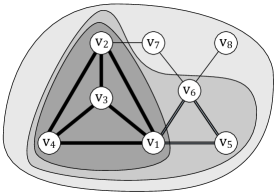
Figure 2: Triangle cores 4, 3, and 2. A $k$ triangle-core is an edge-induced subgraph of $G$ such that each edge participates in $k-2$ triangles. Hence, each clique of size $k$ is contained within a $k$ triangle-core of $G$. Similarly, the $k$ triangle-core is contained within the $(k-1)$-core (i.e., the k-1 core from the k-core decomposition).

The concept of $k$ triangle-core has recently emerged in network analysis research, it was first proposed in Cohen (2009), and improved in Zhang and Parthasarathy (2012); Rossi (2014). A $k$ triangle-core is an edge-induced subgraph of $G$ such that each edge participates in at least $k-2$ triangles and $k\geq 2$. A subgraph $H_{k}=(V|E(F))$ induced by the edge-set $F$ is a maximal triangle core of order $k$ if $\forall(u,v)\in F:tr_{H}(u,v)\geq k-2$, and $H_{k}$ is the maximum subgraph with this property. Most importantly, we define the triangle core number denoted $T(u,v)$ of an edge $e=(u,v)\in E$ to be the highest order $k$ of a maximum triangle $k$-core that $e$ can possibly belong to. See Figure 2 for further intuition. Computing the triangle core numbers of each edge $e$ in the graph $G$ is called the triangle core decomposition of $G$. In Section 3.2, we provide an efficient algorithm for computing the triangle core decomposition with runtime $O(|E|^{3/2})$.

3 Greedy Coloring Framework

In this section, we present a scalable fast framework for coloring large complex networks and introduce the variations designed for the structure of these large complex networks found in the real-world.

3.1 Problem Definition

Let $G=(V,E)$ be an undirected graph. A clique is a set of vertices any two of which are adjacent. The maximum size of a clique in $G$ is denoted $\omega(G)$. An independent set $C$ is a set of vertices any two of which are non-adjacent, thus, $\forall(v,u)\in C$ iff $(v,u)\not\in E$. The graph coloring problem consists of assigning a color to each vertex in a graph $G$ such that no adjacent vertices share the same color, minimizing the number of colors used. More formally,

Definition 3.1 (Graph Coloring Problem):

Given a graph $G$, find a mapping $\phi:V\rightarrow\{1,...,k\}$ where $\phi(v_{i})\not=\phi(v_{j})$ for each edge $(v_{i},v_{j})\in E$. such that $k$ (the number of colors) is minimum.

This problem may also be viewed as a partitioning of vertices $V$ into independent sets $C_{1},C_{2},...,C_{k}$ where $\{1,2,...,k\}$ are called colors and the sets $C_{1},...,C_{k}$ are referred to as color classes. Thus, the graph coloring problem is to find the minimum number $k$ of independent sets (or color classes/partitions) required to color the graph $G$. Nevertheless, graph coloring is NP-hard to solve optimally (on general graphs), and for all $\epsilon>0$, it is even NP-hard to approximate to within $n^{1-\epsilon}$ where $n$ is the number of vertices Garey and Johnson (1979).

In this work, we relax the strict requirement of partitioning the vertices into the minimum number of independent sets to allow for colorings that are close to the optimal. This relaxation gives rise to fast linear-time coloring algorithms that perform well in practice (See Section 6). Motivated by this, we describe general conditions for greedy coloring that can serve as a unifying framework in the study of these algorithms. More formally, we define the greedy coloring framework as follows:

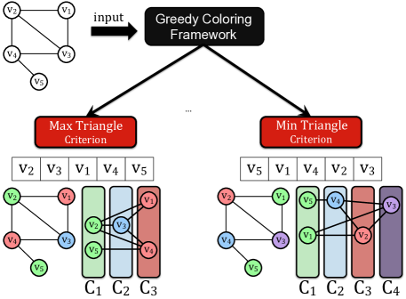
Figure 1: Greedy Coloring Framework. In this graph, we use the number of triangles incident to a vertex $v\in V$ as the selection criterion. On the left, vertices are ordered from largest to smallest using the number of triangles, which results in a greedy coloring that utilizes only three colors. For this graph, this coloring is also optimal and thus $\chi(G,\pi)={\rm\chi}(G)$. However, when vertices are ordered from smallest to largest (on the right) results in a coloring that uses four colors. As an aside, $\Delta(G)+1$ is the maximum number of colors that can be used from any greedy coloring method from the framework and thus ${\rm\chi}(G,\pi)\leq\Delta(G)+1$. In this graph, $\Delta(G)+1=4$ and thus, the ordering used on the right is also the worst possible coloring that can be obtained. Notice that in this example, we used the vertex index as the tie breaking strategy, i.e., $v_{i}$ is ordered before $v_{j}$ if $i<j$. We also note that if the proposed repair coloring scheme (Section 4) were used in the minimum triangle selection criterion, then only three colors would be needed. Other selection criterion (e.g., degree) may lead to a different vertex ranking and as a consequence the greedy coloring framework may result in an entirely different coloring. For instance, ranking the vertices by max degree gives $\{v_{2},v_{3},v_{4},v_{1},v_{5}\}$ which differs from the ranking given by max triangle counts. Further, if two nodes have equal degrees, then we break ties using triangle counts (known as a tie-breaking strategy).

Definition 3.2 (Framework):

Given a graph $G=(V,E)$ and a vertex property $f(\cdot)$, the greedy coloring framework selects the next (uncolored) vertex $v$ to be colored such that

$$v=\operatorname*{arg\,max}_{v_{i}}f(v_{i})$$

The selected vertex $v$ is then assigned to the smallest permissible color. This process is repeated until all vertices are colored.

The main intuition of the greedy coloring framework is to color the vertices that are more constrained in their choice of color as early as possible, giving more freedom to the coloring algorithm to use fewer colors, and thus result in a tighter upper bound on the exact number of colors. As an aside, selecting the vertex that minimizes $f(v)$ usually results in a coloring that uses significantly more colors than the latter. Notice that a fundamental property of the above greedy coloring framework is that it is both fast and efficient, thus, providing us with a natural basis for investigating the coloring of large real-world networks, which is precisely the scope of this work.

The above definition of the framework uses a selection criterion as the basis for coloring. Instead, we replace the selection criterion with the more general notion of a vertex ordering. More specifically, given a graph $G=(V,E)$ and a vertex ordering

$$\pi=\{v_{1},v_{2},...,v_{i},...,v_{n}\}$$

of $V$, let ${\rm\chi}(G,\pi)$ denote the number of colors used by a greedy coloring method that uses the vertex ordering $\pi$ of $G$. Hence, the greedy coloring framework selects the next vertex to color based on the vertex ordering. This formalization allows for a more precise characterization of the framework that depends on three components:

1. A graph property $f(G)$ for selecting the vertices to color

2. The direction in which vertices are selected (e.g., smallest to largest). For instance, $\pi=\{v_{1},...,v_{n}\}$ is from max to min if $f(v_{1})\geq\cdots\geq f(v_{n})$, or min to max if $f(v_{1})\leq\cdots\leq f(v_{n})$.

3. A tie-breaking strategy for the case when the graph property assigns the same value to two vertices. Suppose $f(v)=f(u)$, then $v$ is before $u$ in the ordering $\pi$ if $f^{\star}(v)>f^{\star}(u)$ where $f^{\star}(\cdot)$ is another graph property used to break-ties.

Notice that two vertex orderings $\pi_{1}$ and $\pi_{2}$ from the graph property $f(G)$ may significantly differ in the number of colors used in a greedy coloring (i.e., ${\rm\chi}(G,\pi_{1})\not={\rm\chi}(G,\pi_{2})+\epsilon$). This is due to the direction of the ordering (smallest to largest) and tie-breaking strategy selected. Consequently, a specific graph property $f(\cdot)$ defines a class of orderings where the order direction (from max to min) and tie-breaking strategy ($f^{\star}(\cdot)$) represent a specific member of that class of orderings. Note that in general $f(G)$ can be thought simply as a function for obtaining an ordering $\pi$.

In addition, we also define a few relationships between the graph parameters introduced thus far. Clearly, ${\rm\chi}(G,\pi)$ from a greedy coloring method is an upper bound on the exact number of colors required, denoted by $\chi(G)$, i.e., the minimum number of colors required for coloring $G$. Further, let $\omega(G)$ be the size of the maximum clique in $G$, which is also a lower bound on the minimum number of colors required to color $G$. This gives the following relationship:

$$\omega(G)\leq\chi(G)\leq{\rm\chi}(G,\pi)\leq\Delta(G)+1$$

where $\Delta(G)$ is the maximum degree of $G$.

An example of the framework is shown in Figure 1. This illustration uses a proposed triangle selection criterion, which is shown later in Section 6 to be extremely effective for large social and information networks.

Table 1: Methods used as selection criterion. The previously proposed methods are unified under the framework and categorized into three general classes (i.e., index-based, degree-based methods, and degree distance-2-based methods). Many of these greedy coloring methods are considered the state-of-the-art for small and/or relatively dense graphs from other domains Gebremedhin et al (2013), and thus used as a baseline for evaluating our methods. However, this work proposes three main classes of methods for large complex networks including social-based methods, multi-property methods, and egonet-based methods.

Name	Property   $f(\cdot)$
natural	$f(v)=index(v)$, select next uncolored vertex in the order in which vertices appear in $G$
rand	$f(v)\sim Uni(1,|V|)$, select the next uncolored vertex uniformly at random from the uncolored vertices
Degree distance-1 methods
deg	$f(v)=d(v)$, no. adjacent vertices of $v$ in $G$ (i.e., degree )
dlf	$f(v)=$ no. uncolored adjacent vertices of $v$
ido	$f(v)=$ no. colored adjacent vertices of $v$ (i.e., $|N_{c}(v)|$)
kcore (slo)	$f(v)=K(v)$, k-core number of $v$
Degree distance-2 methods
dist-two-deg	$f(v)=|N_{hops=2}(v)|$, no. unique vertices 2-hops away of $v$ in $G$
dist-two-dlf	$f(v)=$ no. unique uncolored vertices 2-hops away of $v$
dist-two-ido	$f(v)=$ no. unique colored vertices 2-hops away of $v$
Social-based methods
tri	$f(v)=tr(v)$, no. triangles of $v$ in $G$
tcore-max	$f(v)=\max_{w\in N(v)}{\rm T}(v,w)$, triangle core number of $v$
Multi-property methods
kcore-deg	$f(v)=K(v)\cdot d(v)$
tri-deg	$f(v)=tr(v)\cdot d(v)$
tri-kcore	$f(v)=tr(v)\cdot K(v)$
tri-kcore-deg	$f(v)=tr(v)\cdot K(v)\cdot d(v)$
Egonet-based methods
deg-vol	$f(v)=\sum_{w\in N(v)}{\rm d}(w)$
kcore-vol	$f(v)=\sum_{w\in N(v)}{\rm K}(w)$
tri-vol	$f(v)=\sum_{w\in N(v)}tr(w)$
tcore-vol	$f(v)=\sum_{w\in N(v)}{\rm T}(v,w)$
kcore-deg-vol	$f(v)=\sum_{w\in N(v)}tr(w)\cdot d(w)$
tri-kcore-vol	$f(v)=\sum_{w\in N(v)}tr(w)\cdot K(w)$
tri-kc-deg-vol	$f(v)=\sum_{w\in N(v)}tr(w)\cdot K(w)\cdot d(w)$

3.2 Ordering Techniques

In this section, we first review the previous methods used for coloring relatively small and/or dense graphs from other domains (see Gebremedhin et al (2013)), which are unified under our coloring framework. Many are considered state-of-the-art greedy coloring techniques and shown to perform reasonably well for those types of graphs. Despite the past success of these methods, they are not as well suited for large sparse complex networks (e.g., social, information, and technological networks) as demonstrated in this work. As a result, we propose three classes of methods for greedy coloring based on well-known fundamental properties of these large complex networks. In particular, we propose social-based methods, multi-property, and methods based on egonet properties, which are shown later in Section 6 to be more effective than the state-of-the-art techniques used in coloring graphs from other domains. A summary and categorization of these methods are provided in Table 1.

Algorithm 1 Basic Greedy Coloring

1procedure GreedyColoring($G$, $\pi$)

2    Initialize data structures

3    for $v\in\pi$ in order do

4        for $w\in N(v)$ do ${\sf used}({\sf color}(w))\leftarrow v$         

5        $k\leftarrow\min\{i>0:{\sf used}(i)\not=v\}$

6        if $k>\rm\max$ then $\rm\max\leftarrow k$         

7        ${\sf color}(v)\leftarrow k$     

Index-based Methods: The simplest arbitrary ordering techniques under the sequential greedy coloring framework are natural ordering (natural) and random ordering (rand). The natural ordering (natural) method selects the vertices to be colored in their natural order as they appear in the input graph $G$, i.e., $v_{1},v_{2},...,v_{n}$. We also define the random ordering (rand) as the method that selects the vertices to be colored randomly. Therefore, the (rand) method selects a vertex by drawing an uncolored vertex uniformly at random without replacement from $V$.

Degree Methods: The four simplest, yet most popular ordering methods under the sequential greedy coloring framework (Section 3) are all based on vertex degree. Specifically, we use the degree ordering deg, the incidence degree ordering (ido), the dynamic-largest-first (dlf), and the k-core ordering (kcore) (a.k.a smallest-last ordering (slo)). First, the degree ordering (deg) Welsh and Powell (1967) orders vertices from largest to smallest by their static degree as it appears in $G$. Second, the incidence-degree ordering (ido) Coleman and Moré (1983) dynamically orders vertices from largest to smallest by their back degree, such that the back degree of $v$ is the number of its colored neighbors. In this case, the incidence-degree method initially starts with all vertices with back degree equal to zero, and initially selects an arbitrary vertex $v$ to color. Then, all the neighbors of $v$ will increase their back degree by one, and the next vertex with largest back degree will be selected for coloring. This process continues until all vertices are colored. Third, in contrast to the incidence-degree method (ido), the dynamic-largest-first (dlf) Gebremedhin et al (2013) dynamically orders the vertices by their forward degree from largest to smallest, where the forward degree of $v$ is the number of its uncolored neighbors. Thus, the dynamic-largest-first method initially starts with all vertices with forward degree equal to their original degree in $G$, and selects the first vertex $v$ to color, such that $v$ has the maximum degree in $G$ (i.e, $d(v)=\Delta(G)$). Consequently, all the neighbors of $v$ will decrease their forward degree by one, and the vertex with the largest forward degree will be selected next to be colored.

Finally, the $k$-core ordering (kcore) (also known as the smallest-last ordering (slo)  Matula and Beck (1983)) orders the vertices from lowest to highest by their $k$-core number (refer to Section 2 for definition). The $k$-core ordering method (a.k.a smallest-last ordering) was proposed in Matula and Beck (1983), based on the concept of $k$-core decomposition, to find a vertex ordering of a finite graph $G$ that optimizes the coloring number of the ordering in linear time, by repeatedly removing the vertex of smallest degree. The $k$-core ordering dynamically orders the vertices by their forward degree from smallest to largest, where the forward degree of $v$ is the number of its uncolored neighbors. The method initially starts with all vertices with forward degree equal to their original degree in $G$, and selects the first vertex $v$ to color, such that $v$ has the smallest degree in $G$ (i.e, ${\rm d}(v)=\delta(G)$). Thus, all the neighbors of $v$ will decrease their forward degree by one, and the vertex with the next smallest forward degree will be selected for coloring. The output of this method is the vertex ordering for the coloring number, which is equivalent to ordering vertices by their $k$-core number as defined in Szekeres and Wilf (1968).

Table 2: Dynamic Ordering Methods. Summary of the main dynamic degree-based and dynamic triangle-based ordering methods. Note that slt and tcore are used interchangeably. For convenience, let $e$ denote an edge $(v,u)$.

		Operations
Methods		Initialization	Find	Update
Degree	id	${{d_{{{\sf\it b}}}}}(v)=0$	$v=\leavevmode\hbox{\set@color\hskip 7.17685pt\leavevmode\hbox{\set@color$\max$}\raisebox{-6.34833pt}{$\scriptstyle w\in{{V_{{{\sf\it b}}}}}$}\hskip 7.17685pt}\;{{d_{{{\sf\it b}}}}}(w)$	${{d_{{{\sf\it b}}}}}(w)\leftarrow{{d_{{{\sf\it b}}}}}(w)+1$
slo	${{d_{{{\sf\it b}}}}}(v)=d(v)$	$v=\leavevmode\hbox{\set@color\hskip 7.17685pt\leavevmode\hbox{\set@color$\min$}\raisebox{-6.34833pt}{$\scriptstyle w\in{{V_{{{\sf\it b}}}}}$}\hskip 7.17685pt}\;{{d_{{{\sf\it b}}}}}(w)$	${{d_{{{\sf\it b}}}}}(w)\leftarrow{{d_{{{\sf\it b}}}}}(w)-1$
Triangles	it	$T(e_{i})=0$	$e_{i}=\leavevmode\hbox{\set@color\hskip 6.95361pt\leavevmode\hbox{\set@color$\max$}\raisebox{-6.34833pt}{$\scriptstyle e_{j}\in E_{b}$}\hskip 6.95361pt}\;T(e_{j})$	${\rm T}(e_{j})\leftarrow{\rm T}(e_{j})+1$
	slt	$T(e_{i})={\rm tr}(e_{i})$	$e_{i}=\leavevmode\hbox{\set@color\hskip 5.83334pt\leavevmode\hbox{\set@color$\min$}\raisebox{-6.34833pt}{$\scriptstyle e_{j}\in\operatorname{E}_{b}$}\hskip 5.83334pt}\;T(e_{j})$	${\rm T}(e_{j})\leftarrow{\rm T}(e_{j})-1$
lft	$T(e_{i})={\rm tr}(e_{i})$	$e_{i}=\leavevmode\hbox{\set@color\hskip 6.5139pt\leavevmode\hbox{\set@color$\max$}\raisebox{-6.34833pt}{$\scriptstyle e_{j}\in\operatorname{E}_{b}$}\hskip 6.5139pt}\;T(e_{j})$	${\rm T}(e_{j})\leftarrow{\rm T}(e_{j})-1$

These methods (including kcore) were found to be superior to others, especially for forests and a few types of planar graphs Gebremedhin et al (2013). We also use these as baselines for evaluating our proposed methods (see Section 6).

Distance-2 Degree Methods: We note that the degree-based methods were defined on the 1-hop away neighbors of each vertex $v\in V$. These methods can also be extended for the unique 2-hop away neighbors of each vertex $v\in V$ McCormick (1983), we call these methods distance-2 degree ordering (dist-two-deg), distance-2 incidence degree ordering (dist-two-id), distance-2 dynamic largest first ordering (dist-two-dlf), and distance-2 $k$-core ordering (dist-two-kcore) respectively.

Social-based Methods: While the degree-based methods were shown to perform well in the past, in this paper, we compare them to other social-based orderings such as triangle ordering (tri), and triangle-core ordering (tcore).

First, the triangle ordering (tri) method orders vertices from largest to smallest by the number of triangles they participate in, i.e. $f(v)=tr(v)$ where $tr(v)$ can be computed fast and in parallel using Alg 2. Other triangle-based quantities such as clustering coefficient may also be used and computed fast and efficiently using Alg 2. Thus, the triangle ordering initially selects the vertex $v$ with the largest number of triangles centered around it. This process continues until all vertices are colored. The intuition behind triangles in social networks is that vertices tend to cluster, and therefore, triangles were extensively used to measure the number of vertices adjacent to $v$ that are also linked together (as explained in Section 2). We conjecture that ordering vertices from largest to smallest by their triangle number would give a chance to those vertices that are more constrained in their choices of color to be colored first than those that have more freedom (as we explained earlier).

Algorithm 2 Parallel Vertex Triangle Counting

1procedure ParallelVertexTriangles($G=\left(V,E\right)$)

2    Initialize arrays

3    for each $v\in V$ in parallel do

4        for each $u\in N(v)$ do $X(u)\leftarrow v$ $\triangleright$ s.t. $v>0$         

5        for each $u\in N(v)$ do

6           for each $w\in N(u)$ do

7               if $v=w$ then continue                

8               if $X(w)=v$ then ${\rm tr}(v)\leftarrow{\rm tr}(v)+1$                                       

Second, the triangle-core ordering (tcore) method orders vertices from largest to smallest by their triangle core number (as explained in Section 2). Using the triangle core numbers, we obtain an ordering and use it to determine the next vertex $v$ (or edge) to color, using the criteria: $f(v)=\max_{w\in N(v)}{\rm T}(v,w)$, where $N(v)$ is the set of neighbors of vertex $v$, and ${\rm T}(v,w)$ is the triangle core number of the edge $(v,w)\in E$. Notice that triangle core ordering is comparable to $k$-core ordering, however, instead of removing a vertex and its edges at each iteration, we remove an edge and its triangles. This gives rise to a variety of ordering methods based on the fundamental notion of removing edges and their triangles. We call these dynamic triangle ordering methods and provide a summary of the main ones in Table 2 as well as a comparison with a few of the dynamic degree-based methods. Let us note that any edge-based quantity may be used for ordering vertices (and vice-versa). For instance, tcore-max defined in Table 1 computes for every vertex $v$ in the graph, the maximum triangle core number among the (1-hop)-away-neighbors of $v$.

The proposed triangle ordering template is shown in Alg 3 and the key operations are also summarized in Table 2. The backward (or forward) triangle counts are initialized in Line 2. For slt, ParallelEdgeTriangles shown in Alg 4 is used to initialize the triangle counts. Next, line 3 adds $(v,u)$ to the bucket consisting of the edges with $T(v,u)$ triangles which is denoted $\mathtt{bin}[T(v,u)]$. Hence, the edges are ordered in $O(|E|)$ time using a bucket sort. Note that if it is used then this step can be skipped since each edge $(v,u)$ is initialized as $T(v,u)=0$.

The triangle ordering begins in line 4 by ensuring $|E|>0$ where $E$ initially consists of all edges in $G$. At each iteration, a single edge $(v,u)$ is removed from $E$. Line 5 finds the edge $(v,u)$ with the smallest $T(v,u)$ or largest $T(v,u)$, see Table 2 for the variants. The neighbors of $u$ that remain in $E$ are marked in line 7 with the unique edge identifier $e_{i}$ of $(v,u)$ (to avoid resetting the array). In line 8, we iterate over the triangles that $(v,u)$ participates, i.e., the pairs of edges $(v,w)$ and $(u,w)$ that form a triangle with $(v,u)$. Since the neighbors of $u$ are marked in $X$, then a triangle is verified by checking if each neighbor $w$ of $v$ has been marked in $X$, if so then $u,v,w$ must form a triangle. Line 9 sets $\mathtt{bin}[T(v,w)]\leftarrow\mathtt{bin}[T(v,w)]\setminus(v,w)$ and $\mathtt{bin}[T(u,w)]\leftarrow\mathtt{bin}[T(u,w)]\setminus(u,w)$, removing $(v,w)$ and $(u,w)$ from their previous bins. Next, the triangle counts of $(v,w)$ and $(u,w)$ are updated in line 10 using an update rule from Table 2. Afterwards, line 11 adds the edges to the appropriate bin, i.e., $\mathtt{bin}[T(v,w)]\leftarrow\mathtt{bin}[T(v,w)]\cup(v,w)$ and $\mathtt{bin}[T(u,w)]\leftarrow\mathtt{bin}[T(u,w)]\cup(u,w)$. This is repeated for each pair of edges $(v,w)$ and $(u,w)$ that form a triangle with $(v,u)$. Finally, line 12 implicitly removes the edge $(v,u)$ from $E$.

Algorithm 3 Dynamic Triangle Ordering Template

1for each $(v,u)\in E$ in parallel do

2    $T(v,u)\leftarrow\textsf{Initialize}(v,u)$

3    $\mathtt{bin}[T(v,u)]\leftarrow\mathtt{bin}[T(v,u)]\cup(v,u)$

4while $|E|>0$ do

5    Find the edge $(v,u)$ with $\min\{T(v,u)\}$ (or $\max\{T(v,u)\}$)

6    Add the edge $(v,u)$ to the back of $\pi$

7    for each $w\in N(v)$ that remain do $X(w)\leftarrow e_{i}$     

8    for each $w\in N(u)$ such that $X(w)=e_{i}$ do

9        Remove $(v,w)$ and $(u,w)$ from $\mathtt{bin}$

10        Update $T(v,w)$ and $T(u,w)$

11        Add $(v,w)$ and $(u,w)$ to the appropriate bin     

12    $E\leftarrow E\setminus\{(v,u)\}$

13end while

14return $\pi$

Algorithm 4 Parallel Edge Triangle Counting

1procedure ParallelEdgeTriangles($G=\left(V,E\right)$)

2    Initialize arrays

3    for each $(v,u)\in E$ in parallel do

4        for each $w\in N(v)$ do $X(w)\leftarrow\text{edge pos of (v,u)}$         

5        for each $w\in N(u)$ do

6           if $v=w$ then continue            

7           if $X(w)=\text{edge pos of (v,u)}$ then

8               ${\rm tr}(v,u)\leftarrow{\rm tr}(v,u)+1$                        

Egonet-based Methods: An egonet is the induced subgraph centered around a vertex $v$ and consists of $v$ and all its neighbors $N(v)$. Assume we are given an arbitrary graph property $f(\cdot)$ (e.g., triangle-cores, number of triangles) computed over the set of neighbors of $v$, i.e., $N(v)$, we define an egonet ordering criterion for a vertex $v$ as $\sum_{w\in N(v)}f(w)$. In addition, besides using the ${\rm sum}$ operator over the egonet, one may use other relational aggregators such as $\min$, ${\rm max}$, ${\rm var}$, ${\rm avg}$, among many others.

Multi-property Methods: We also propose ordering techniques that utilize multiple graph properties. For instance, the vertex to be colored next may be selected based on the product of the vertex degree and $k$-core number, i.e., $f(v)=K(v)\cdot d(v)$.

3.3 Algorithm and Implementation

This section describes the algorithms and implementation. The graph is stored using $O(|E|+|V|)$ space in a structure similar to Compressed Sparse Column (CSC) format used for sparse matrices Tewarson (1973). If the graph is small and/or dense enough, then it is also stored as an adjacency matrix for constant time edge lookups. Besides the graph, the algorithm uses two additional data structures. In particular, let ${\sf color}$ be an array of length $n$ that stores the color assigned to each vertex, i.e., ${\sf color}(v)$ returns the color class assigned to $v$. Additionally, we also have another array to mark the colors that have been assigned to the neighbors of a given vertex and thus we denote it as ${\sf used}$ to refer to the colors “used” by the neighbors.

The algorithmic framework for greedy coloring is shown in Alg 1. For the purpose of generalization, we assume the vertex ordering $\pi$ is given as input and computed using a technique from Section 3.2.

The algorithm starts by initializing each entry of ${\sf color}$ with $0$. We also initialize each of the entries in ${\sf used}$ to be an integer $x\not\in V$ (i.e., an integer that does not match a vertex id). The greedy algorithm starts by selecting the next vertex $v_{i}$ in the ordering $\pi$ to color. For each vertex $v_{i}$ in order, we first iterate over the neighbors of $v_{i}$ denoted $w\in N(v)$, and set ${\sf used}({\sf color}(w))=v_{i}$ as shown in Line 4. This essentially marks the colors that have been used by the neighbors. Afterwards, we sequentially search for the minimal $k$ such that ${\sf used}(k)\not=v_{i}$ (in Line 7). Line 5 assigns this color to $v_{i}$, hence ${\sf color}(v_{i})=k$. Upon termination, ${\sf color}$ is a valid coloring and the number of colors is ${\rm\chi}(G,\pi)=\operatorname*{arg\,max}_{v\in P}{\sf color}(v)$. We denote ${\rm\chi}(G,\pi)$ as the number of colors from a greedy coloring algorithm that uses the ordering $\pi$ of $V$, which is easily computed in $O(1)$ time by maintaining the max color assigned to any vertex.

Note that in Line 4, the color of $w$ (a positive integer) is given as an index into the ${\sf used}$ array and marked with the label of vertex $v_{i}$. This trick allows us to avoid re-initializing the ${\sf used}$ array after each iteration over a vertex $v_{i}\in\pi$ – the outer for loop. Hence, if $w$ has not yet been assigned a color, i.e., ${\sf color}(w)=0$, then $used(0)$ is assigned the label of $v_{i}$, and since $0$ is an invalid color, it is effectively ignored. In addition, each entry in ${\sf used}(k)$, $1\leq k\leq\Delta+1$ must initially be assigned an integer $x\not\in\pi$.

3.4 Complexity

The storage cost is only linear in the size of the graph, since CSC takes $O(|E|+|V|)$ space, the vertex-indexed array ${\sf color}$ costs $O(|V|)$, and ${\sf used}$ costs $O(\Delta+1)$ space. For the ordering methods, degree and random take $O(|V|)$ time, whereas the other “dynamic degree-based” techniques such as kcore have a runtime of $O(|E|)$ time. The other ordering techniques that utilize triangles and triangle-cores take $O(|E|^{3/2})$ time in the worst-case, but are shown to be much faster in practice. Importantly, we also parallelize the triangle-based ordering methods by computing triangles independently for each vertex or edge. We also note the distance two ordering methods are just as hard as the triangle ordering methods, yet perform much worse as shown in Section 6. Finally, the greedy coloring framework has a runtime of $O(|V|+|E|)$ and $O(|E|)$ for connected graphs.

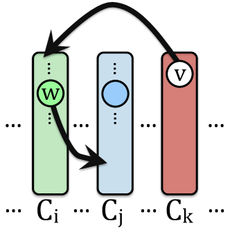
Figure 3: Repair Coloring. Suppose $v$ is the vertex to be recolored since it is assigned to a new color class $C_{k}$, then we find a color class $C_{i}$ where $v$ is adjacent to a single vertex $w$ (i.e., $N(v)\cap C_{i}=\{w\}$). Now, we find a color class $C_{j}$ s.t. $j>i$ and $w$ is not adjacent to any vertex in $C_{j}$, i.e. $|N(w)\cap C_{j}|=\emptyset$. If such a color class exists, then $w$ is removed from $C_{i}$ and assigned to $C_{j}$. As a result of this reassignment, $v$ can now be assigned to the $C_{i}$ color class, therefore reducing the number of colors by 1.

4 Recolor Variant

This section proposes another coloring variant that attempts to recolor vertices to reduce the number of colors. The variant is effective while also fast for large real-world networks.

4.1 Algorithm

The recoloring variant is shown in Alg. 5. This variant proceeds in a similar manner as the basic coloring algorithm from Section 3.3. The difference is that if a vertex is assigned an entirely new color $k$ (i.e., number of colors used in the coloring increases), then an attempt is made to reduce the number of colors. Using this as a basis for recolor ensures that the algorithm is fast, taking advantage of only the most promising situations that arise.

Suppose the next vertex $v$ in the ordering is assigned a new color $k$ and thus $C_{k}=\{v\}$, then we attempt to reduce the number of colors by reassigning an adjacent vertex $u$ that was assigned a previous color $i$ such that $i<k$. Hence, if $|C_{i}\cap N(v)|=1$, then $C_{i}$ contains a single adjacent vertex of $v$ (i.e., a single conflict), and thus, we attempt to recolor $u$ by assigning it to the minimum color $j$ such that $i<j<k$ and $C_{j}\cap N(u)=\emptyset$. This arises due to the nature of the sequential greedy coloring and is formalized as follows: Given vertices $v$ and $u$ assigned to the $i^{th}$ and the $j^{th}$ colors, respectively, where $v$ is colored first and $i<j$, then since $v$ is assigned the minimum possible color, then we know the colors less than $i$ are invalid, however, $v$ could potentially be assigned the colors $i+1,...,k$, since these colors arose after $v$ was assigned a color.

The key intuition of the recolor variant is illustrated in Figure 3. In the start of the example, notice that $v$ is assigned to a new color class $C_{k}$ (i.e., contains only $v$). Therefore, the recolor method is called, which attempts to find $v$ another color class denoted $C_{i}$ where $C_{i}<C_{k}$. For this, we search for a color class $C_{i}$ that contains a single adjacent vertex denoted $w$ (known as a conflict). Intuitively, we may assign $v$ to $C_{i}$ if we can find $w$ another “valid” color class denoted $C_{j}$. Notice that $i<j<k$ such that the color class $C_{i}$ appeared before $C_{j}$ and so forth. In other words, $v$ can be assigned to $C_{i}$ if there exists a valid color class $C_{j}$ for which $w$ can be assigned. If such a $C_{j}$ exists, then the number of colors is decreased by one.

Algorithm 5 Fast Greedy Recoloring

1procedure GreedyRecolor($G$, $\pi$)

2    Initialize data structures

3    for $v\in\pi$ in order do

4        for $w\in N(v)$ do ${\sf used}({\sf color}(w))\leftarrow v$         

5        $k\leftarrow\min\{i>0:{\sf used}(i)\not=v\}$

6        ${\sf color}(v)\leftarrow k$

7        if $k>\rm\max$ then

8           if recolor(${\sf color}$, $v$, $k$) then $k\leftarrow k-1$            

9           $\rm\max\leftarrow k$              

10procedure recolor(${\sf color}$, $v$, $k$)

11    Initialize conflicts to be $0$

12    for $w\in N(v)$ do

13        $\mathsf{conflicts}({\sf color}(w))\leftarrow\mathsf{conflicts}({\sf color}(w))+1$

14        ${\sf used}({\sf color}(w))\leftarrow w$     

15    for $i=1$ to $(k-1)$ do

16        if $\mathsf{conflicts}(i)=1$ then

17           $w\leftarrow{\sf used}(i)$

18           for $u\in N(w)$ do ${\sf used}({\sf color}(u))\leftarrow w$            

19           $c\leftarrow\min\{j>i:{\sf used}(j)\not=w\}$

20           if $c<{\sf color}(v)$ then

21               ${\sf color}(v)\leftarrow{\sf color}(w)$ and ${\sf color}(w)\leftarrow c$

22               return true                        

23    return false

5 Bounds

Lower and upper bounds on the minimum number of colors are useful for a number of reasons (see Section 6.4). In this section, we first provide a fast parallel method for computing a lower bound that is especially tight for large sparse networks. Next, we summarize the upper bounds used in this work, which are also shown to be strong, and in many cases matching that of the lower bound, and thus allowing us to verify the coloring from one of our methods.

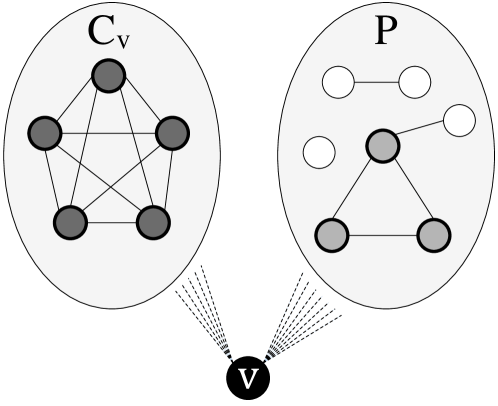
Figure 4: Clique Invariant and Fast Heuristic Clique Finder. Recall $C_{v}$ is the clique being constructed, whereas $P$ is the set of potential vertices that could be added to $C_{v}$ to form a clique of $|C_{v}|+1$. Further, after a vertex $u$ from $P$ is added to $C_{v}$, we must then remove $u$ from $P$ and compute the intersection $P\cap N_{R}(u)$. The result of this intersection depends intrinsically on how well $u$ is connected to the vertices in $P$. In the ideal case, the heuristic is guaranteed to find the largest possible clique as long as the vertices in $P$ that form the largest clique among each other are added to $C_{v}$. For instance, the largest clique in the above example is $|C_{v}|+3=8$ formed by adding the three vertices forming a 3-clique (triangle) in $P$ to $C_{v}$, whereas if $u\in P$ with 0 degree is added to $C_{v}$, then $|C_{v}|+1=6$, since $P_{t}\cap N_{R}(u)=\emptyset$.

5.1 Lower Bounds

Let $\tilde{\omega}(G)$ be the size of a large clique from a heuristic clique finder and thus a lower-bound on the size of the maximum clique $\omega(G)$. As previously mentioned, $\tilde{\omega}(G)\leq\omega(G)\leq\chi(G)$. Since the maximum clique problem is known to be NP-hard, we use a fast parallel heuristic clique finder tuned specifically for large sparse complex networks. Our approach is shown in Alg. 6 and found to be efficient while also useful for obtaining a large clique that is often of maximum or near-optimal size (i.e., $\tilde{\omega}(G)$ is close to $\omega(G)$) for many types of large real-world networks.

Given a graph $G=(V,E)$, the heuristic obtains a vertex ordering $\pi=\{v_{1},...,v_{n}\}$ and searches each vertex $v_{i}$ in the ordering $\pi$ for a large clique in $N(v_{i})$. For convenience, let $N_{R}(v)$ be the reduced neighborhood of $v$ defined formally as,

$$N_{R}(v)=G(\{v\}\cup\{u:(u,v)\in E,B(u)\geq|C_{\max}|,u\not\in X)\}$$

where $|C_{\max}|$ is the largest clique found thus far, $B(u)$ is a vertex upper bound, and ${{\rm X}}$ is a vertex-index array of pruned vertices (i.e., $O(1)$ time check). Thus, let $P\leftarrow N_{R}(v)$ be the set of potential vertices and initially we set $C_{v}\leftarrow\emptyset$. At each step in the heuristic, a vertex $u\in P$ is selected according to a greedy selection criterion $f(\cdot)$ such that $u\leftarrow\max_{w\in P}f(w)$ where $f(\cdot)$ is a graph property. The selected vertex $u$ is added to $C_{v}\leftarrow C_{v}\cup\{u\}$ and $P_{t+1}\leftarrow P_{t}\cap N_{R}(u)$ where $t$ denotes the iteration (or depth of the search tree). The local clique search terminates if $|P_{t}|+|C_{v}|\leq C_{max}$, since this indicates that a clique of a larger size cannot be found from searching further. See Figure 4 for a simple example. Notice that $C_{v}$ is the clique being built and grows by a single vertex each iteration, whereas $P_{t+1}$ are the potential vertices remaining after adding $u$ to $C_{v}$. Hence, $|P_{t+1}|<|P_{t}|<|P_{t-1}|$ is monotonically decreasing with respect to $t$. It is clear from Figure 4 that $|P_{t+1}|$ and thus the size of the clique $|C_{v}|$ strongly depends on $u$ selected by the greedy selection criterion. In Figure 4, suppose the vertex without edges to other vertices in $P$ is selected and added to $C_{v}$, then $P_{t+1}\leftarrow\emptyset$ and the search terminates. The proposed heuristic clique finder is equivalent to searching down a single branch in a greedy fashion.

Let us also point out that Alg. 6 is extremely flexible. For instance, the vertices in $G$ (globally) and $P$ (locally) are ordered by their k-core numbers (see Line 3 and 7), but any ordering from Table 1 may be used. In addition, while Alg. 6 is presented using vertex k-core numbers for pruning (Line 5), one may also leverage stronger bounds such as the triangle-core numbers (See Rossi (2014)). We used k-core numbers for ordering and pruning since these are relatively tight bounds while also efficient to compute for large networks. Later in Section 6, we demonstrate the tightness of these bounds on large sparse real-world networks (See Table 3 and 4).

Algorithm 6 Fast Heuristic Clique Finder

1procedure HeuristicClique($G=\left(V,E\right),K$)

2    Set $C_{\max}=\{\}$

3    for each $v\in V$ in decr. k-core order in $\mathbf{parallel}$ do

4         if ${\rm K}(v)\geq|C_{\max}|$ then

5             Let $P$ be the neighs. of $v$ with core numbers $\geq$ $|C_{\max}|$

6             Set $C_{v}=\{\}$

7             for each vertex $u\in P$ by decreasing core number do

8                 if $C_{v}\cup\{u\}$ is a clique then

9                     Add $u$ to $C_{v}$                               

10             if $|C_{v}|>|C_{\max}|$ then

11                 Set $C_{\max}=C_{v}$                           

12    return $C_{\max}$, a large clique in $G$

Complexity: The runtime of the heuristic is $O(|E|\cdot{\rm K}(G))$ since it takes $\sum_{v\in V}{\rm d}(v)=2|E|=O(|E|)$ to form the initial set of neighbors for each vertex. The HeuristicClique is essentially a greedy depth-first search where the depth is at most ${\rm K}(G)$. As an aside, if ${\rm T}(G)$ is used instead, then the heuristic is computed in $O(|E|\cdot{\rm T}(G))$. Observe that at each step, the greedy selection criterion $u\leftarrow\max_{v\in P}f(v)$ is evaluated in $O(1)$ time by pre-ordering the vertices prior to searching. The runtime of the ordering is $O(|P|)$ using bucket sort. A global bound on the depth of the search tree for any vertex neighborhood is clearly ${\rm K}(G)$ and for a specific vertex $v$ is no larger than ${\rm K}(v)$. In practice, the heuristic is fast and usually terminates after only a few iterations due to the removal of vertices from $P$ via the strong upper bounds.

Parallel Algorithm The vertex neighborhoods are searched in $\mathsf{parallel}$ for a large clique. Each worker (i.e., processing unit, core) is assigned dynamically a block $\beta$ of vertices to search. The workers maintain a vertex neighborhood subgraph for the vertex currently being searched. In addition, the workers share a vertex-indexed array $X$ of pruned vertices and the largest clique $C_{\max}$ found among all the workers. If a worker finds a clique $C_{v}$ larger than $C_{\max}$, i.e., $|C_{v}|>|C_{\max}|$ (max so far among all workers), then a lock is obtained, and $C_{\max}\leftarrow C_{v}$ and the updated $C_{\max}$ is immediately sent to all workers. As an aside, this immediate sharing of $C_{\max}$ typically leads to a significant speedup, since the updated $C_{\max}$ allows for the workers to further prune their search space including entire vertices.

5.2 Upper Bounds

A simple, but not very useful upper bound on the Chromatic number $\chi(G)$ is given by the maximum degree: $\chi(G)\leq\Delta(G)+1$. A stronger upper bound is given by the maximum k-core number of $G$ denoted by ${\rm K}(G)$. This gives the following relationship:

$$\chi(G)\leq{\rm K}(G)+1\leq\Delta(G)+1$$

In this work, we observe that this upper bound is significantly stronger than the maximum degree on nearly all large sparse networks.

Since ${\rm\chi}(G,\pi)$ depends on an ordering $\pi$ then no relationship exists between ${\rm\chi}(G,{{\textsc{slo}}})$ from slo and ${\rm\chi}(G,\pi)$ where $\pi$ gave rise to ${{\theta_{\pi}}}(G)$. Nevertheless, suppose the vertices are colored using slo resulting in ${\rm\chi}(G,\pi)$ colors, then using ${\rm K}(G)$ gives the following relationship:

$$\tilde{\omega}(G)\leq\omega(G)\leq\chi(G)\leq{\rm\chi}(G,\pi)\leq{\rm K}(G)+1\leq\Delta(G)+1$$

where $\omega(G)$ is the maximum clique in $G$ and $\tilde{\omega}(G)$ is a large clique in $G$ from the fast heuristic clique finder in Section 5.1. In other words, if a greedy coloring method uses $\pi$ from slo then the resulting coloring of $G$ must use at most ${\rm K}(G)+1$ colors. Furthermore, ${\rm K}(G)+1$ is also known as the coloring number denoted ${{\sf col}}(G)$ Erdős and Hajnal (1966).

The above relationship can be further strengthened using the notion of the maximum triangle core number of $G$ denoted ${\rm T}(G)$. This gives rise to the following relationship:

$$\omega(G)\leq\chi(G)\leq{\rm T}(G)\leq{\rm K}(G)+1\leq\Delta(G)+1$$

Table 3: Network Statistics and Coloring Bounds. From the large collection of 100+ graphs used in our experiments, we selected a small representative set from the various types (e.g., web, social networks) to study relationships between key network statistics and lower and upper bounds on the Chromatic number. Here, $\rho$ is the density, $\bar{d}$ is the average degree, and ${\rm r}$ is the assortativity coefficient. We also study the following triangle related statistics: $\kappa$ is the global clustering coefficient, $|T|$ is the total number of triangles, and $tr_{\rm avg}$ and $tr_{\rm\max}$ are the maximum and average number of triangles incident on a vertex, respectively. Using these fundamental network statistics as a basis, we analyze the relationships between these characteristic network properties and our derived bounds on the Chromatic number. The lower bound from the heuristic clique finder is denoted $\tilde{\omega}$. For the upper bounds, we denote $K$ as the maximum k-core (i.e., the largest degree for a $k$-core to exist), and similarly, we also upper bound the Chromatic number using the notion of the maximum triangle-core, which we denote by $T$. Finally, we also include the maximum and minimum number of colors from a coloring method in our framework, which we denote ${\rm\chi}_{\max}$ and ${\rm\chi}_{\min}$, respectively.

		Graph measures							Bounds				Colors
	graph	$|V|$	$|E|$	$|T|$	$\bar{d}$	${\rm r}$	$\kappa$	${\rm tr}_{\rm max}$	$\Delta$	$K$+1	$T$	$\tilde{\omega}$	${\rm\chi}_{\min}$	${\rm\chi}_{\max}$
bio	bio-celegans	453	2K	9.8K	8	-0.23	0.12	870	237	11	9	9	10	16
	bio-diseasome	516	1.1K	4K	4	0.07	0.43	152	50	11	11	10	11	12
	bio-dmela	7.3K	25.5K	8.6K	6	-0.05	0.01	225	190	12	7	7	8	15
	bio-yeast	1.4K	1.9K	618	2	-0.21	0.05	18	56	6	6	5	6	8
collaboration	ca-AstroPh	17.9K	196.9K	4M	22	0.20	0.32	11.2K	504	57	57	56	57	64
	ca-CSphd	1.8K	1.7K	24	1	-0.20	0.00	4	46	3	3	3	3	5
	ca-CondMat	21.3K	91.2K	513.1K	8	0.13	0.26	1.6K	279	26	26	26	26	29
	ca-Erdos992	6.1K	7.5K	4.8K	2	-0.44	0.04	99	61	8	8	8	8	12
	ca-GrQc	4.1K	13.4K	143.3K	6	0.64	0.63	1.1K	81	44	44	44	44	45
	ca-HepPh	11.2K	117.6K	10M	20	0.63	0.66	39.6K	491	239	239	239	239	239
	ca-MathSciNet	332.6K	820.6K	1.7M	4	0.10	0.14	1.5K	496	25	25	25	25	28
	ca-citeseer	227.3K	814.1K	8.1M	7	0.07	0.46	5.3K	1.3K	87	87	87	87	87
	ca-dblp10	226.4K	716.4K	4.7M	6	0.30	0.38	5.9K	238	75	75	75	75	75
	ca-dblp12	317K	1M	6.6M	6	0.27	0.31	8.3K	343	114	114	114	114	114
	ca-hollywood09	1M	56.3M	14.7T	105	0.35	0.31	3.9M	11.4K	2209	2209	2209	2209	2209
	ca-netscience	379	914	2.7K	4	-0.08	0.43	75	34	9	9	9	9	9
	ca-sandi-auths	86	124	126	2	-0.26	0.27	7	12	5	5	4	5	6
interaction	ia-email-EU	32.4K	54.3K	146.9K	3	-0.38	0.03	1.6K	623	23	13	11	16	27
	ia-email-univ	1.1K	5.4K	16K	9	0.08	0.17	261	71	12	12	12	12	15
	ia-enron-large	33.6K	180.8K	2.1M	10	-0.12	0.09	17.7K	1.3K	44	22	15	28	57
	ia-enron-only	143	623	2.6K	8	-0.02	0.36	125	42	10	8	8	8	11
	ia-fb-messages	1.2K	6.4K	7.4K	10	-0.08	0.04	242	112	12	5	5	8	15
	ia-infect-dublin	410	2.7K	21.3K	13	0.23	0.44	280	50	18	16	16	16	18
	ia-infect-hyper	113	2.1K	50.6K	38	-0.12	0.50	1.7K	98	29	18	15	19	28
	ia-reality	6.8K	7.6K	1.2K	2	-0.68	0.00	52	261	6	5	4	5	7
	ia-wiki-Talk	92.1K	360.7K	2.5M	7	-0.03	0.05	17.6K	1.2K	59	20	9	30	64
infra	inf-USAir97	332	2.1K	36.5K	12	-0.21	0.40	1.4K	139	27	22	22	22	31
	inf-power	4.9K	6.5K	1.9K	2	0.00	0.10	21	19	6	6	6	6	7
	inf-roadNet-CA	1.9M	2.7M	361.4K	2	0.12	0.06	7	12	4	4	4	5	6
	inf-roadNet-PA	1M	1.5M	201.3K	2	0.12	0.06	8	9	4	4	3	4	6
misc	ASIC-320ks	321.6K	1.5M	5.9M	9	-0.05	0.11	2.2K	822	9	18	5	6	8
	IMDB-bi	896.3K	3.7M	13K	8	-0.05	0.00	78	1.5K	24	3	3	11	24
	Reuters911	13.3K	148K	3.5M	22	-0.11	0.11	69.8K	2.2K	74	40	26	38	77
	football	115	613	2.4K	10	0.16	0.41	32	12	9	9	9	9	10
	lesmis	77	254	1.4K	6	-0.17	0.50	82	36	10	10	10	10	12
	rec-amazon	91.8K	125.7K	103K	2	0.19	0.35	9	5	5	5	5	5	5
rt	rt-retweet-crawl	1.1M	2.2M	525.9K	4	-0.02	0.00	1.5K	5K	19	13	13	13	23
	rt-retweet	96	117	36	2	-0.18	0.07	6	17	4	4	4	4	5
	rt-twitter-copen	761	1K	447	2	-0.10	0.06	27	37	5	4	4	5	8

Table 4: Network Statistics and Coloring Bounds (continued from Table 3).

		Graph measures							Bounds				Colors
	graph	$|V|$	$|E|$	$|T|$	$\bar{d}$	${\rm r}$	$\kappa$	${\rm tr}_{\rm max}$	$\Delta$	$K$+1	$T$	$\tilde{\omega}$	${\rm\chi}_{\min}$	${\rm\chi}_{\max}$
social networks	soc-BlogCatalog	88.7K	2M	153M	47	-0.23	0.06	804.4K	9.4K	222	101	24	87	170
	soc-FourSquare	639K	3.2M	64.9M	10	-0.71	0.00	1.9M	106.2K	64	38	25	34	47
	soc-LiveMocha	104.1K	2.1M	10M	42	-0.15	0.01	36.9K	2.9K	93	27	10	34	76
	soc-brightkite	56.7K	212.9K	1.4M	7	0.01	0.11	11.5K	1.1K	53	43	31	39	56
	soc-buzznet	101.1K	2.7M	92.7M	54	2.85	0.03	1M	64.2K	154	59	21	62	125
	soc-delicious	536.1K	1.3M	1.4M	5	-0.07	0.01	8K	3.2K	34	23	17	21	35
	soc-digg	770.7K	5.9M	188M	15	-0.09	0.05	396K	17.6K	237	73	41	64	127
	soc-dolphins	62	159	285	5	-0.04	0.31	17	12	5	5	5	5	7
	soc-douban	154.9K	327.1K	121K	4	-0.18	0.01	394	287	16	11	8	13	19
	soc-epinions	26.5K	100.1K	479K	7	0.06	0.09	5.1K	443	33	18	14	20	39
	soc-flickr	513.9K	3.1M	176M	12	0.16	0.15	524K	4.3K	310	153	21	104	208
	soc-flixster	2.5M	7.9M	23.6M	6	-0.32	0.01	15.1K	1.4K	69	47	29	40	75
	soc-gowalla	196.5K	950K	6.8M	9	-0.03	0.02	93.8K	14.7K	52	29	29	29	64
	soc-karate	34	78	135	4	-0.48	0.26	18	17	5	5	5	5	6
	soc-lastfm	1.1M	4.5M	11.8M	7	-0.14	0.01	38K	5.1K	71	23	14	24	57
	soc-livejournal	4M	27.9M	250.6M	13	0.27	0.14	79.7K	2.6K	214	214	214	214	218
	soc-orkut	2.9M	106.3M	1.5T	70	0.02	0.04	1.3M	27.4K	231	75	37	83	190
	soc-pokec	1.6M	22.3M	97.6M	27	0.00	0.05	29.2K	14.8K	48	29	29	30	62
	soc-slashdot	70K	358.6K	1.2M	10	-0.07	0.03	13.3K	2.5K	54	35	17	34	60
	soc-twitter-follows	404.7K	713K	88.6K	3	-0.88	0.00	1.6K	626	29	6	6	7	14
	soc-wiki-Vote	889	2.9K	6.3K	6	-0.03	0.13	251	102	10	7	7	7	15
	soc-youtube-snap	1.1M	2.9M	9.1M	5	-0.04	0.01	180K	28.7K	52	19	13	30	64
	soc-youtube	495K	1.9M	7.3M	7	-0.03	0.01	151K	25.4K	50	19	11	28	61
facebook networks	fb-A-anon	3M	23.6M	166M	15	-0.06	0.05	50.2K	4.9K	75	30	23	33	69
	fb-B-anon	2.9M	20.9M	155.9M	14	-0.11	0.05	36.8K	4.3K	64	31	23	29	60
	fb-Berkeley13	22.9K	852.4K	16.1M	74	0.01	0.11	69.5K	3.4K	65	47	39	48	84
	fb-CMU	6.6K	249.9K	6.9M	75	0.12	0.19	24K	840	70	45	42	49	83
	fb-Duke14	9.8K	506.4K	15.4M	102	0.07	0.17	41.9K	1.8K	86	47	29	47	85
	fb-Indiana	29.7K	1.3M	28.1M	87	0.13	0.14	37.2K	1.3K	77	53	43	52	91
	fb-MIT	6.4K	251.2K	7.1M	78	0.12	0.18	27.7K	708	73	41	30	44	78
	fb-OR	63.3K	816.8K	10.5M	25	0.18	0.15	19.4K	1K	53	36	28	36	63
	fb-Penn94	41.5K	1.3M	21.6M	65	-0.00	0.10	68K	4.4K	63	48	43	47	78
	fb-Stanford3	11.5K	568.3K	17.5M	98	0.10	0.16	33.1K	1.1K	92	60	47	58	90
	fb-Texas84	36.3K	1.5M	33.5M	87	-0.00	0.10	141K	6.3K	82	62	44	57	100
	fb-UCLA	20.4K	747.6K	15.3M	73	0.14	0.14	17.5K	1.1K	66	54	49	53	78
	fb-UCSB37	14.9K	482.2K	9.2M	64	0.18	0.16	16.1K	810	66	60	51	56	78
	fb-UConn	17.2K	604.8K	10.2M	70	0.09	0.13	21.5K	1.7K	66	53	47	51	75
	fb-UF	35.1K	1.4M	36.4M	83	-0.01	0.12	159K	8.2K	84	67	51	61	100
	fb-UIllinois	30.7K	1.2M	28M	82	0.03	0.14	66.1K	4.6K	86	65	54	59	88
	fb-Wisconsin87	23.8K	835.9K	14.5M	70	-0.00	0.12	46.7K	3.4K	61	42	34	42	71
technological	tech-RL-caida	190K	607K	1.3M	6	0.02	0.06	6K	1K	33	19	15	18	34
	tech-WHOIS	7.4K	56.9K	2.3M	15	-0.04	0.31	22.2K	1K	89	71	49	66	88
	tech-as-caida07	26.4K	53.3K	109K	4	-0.19	0.01	3.8K	2.6K	23	16	9	18	30
	tech-as-skitter	1.6M	11M	86.3M	13	-0.08	0.01	564.6K	35.4K	112	68	41	70	115
	tech-internet-as	40.1K	85.1K	189K	4	-0.18	0.01	8.5K	3.3K	24	17	14	18	28
	tech-p2p-gnutella	62.5K	147K	6K	4	-0.09	0.00	17	95	7	4	4	7	11
	tech-routers-rf	2.1K	6.6K	31.2K	6	0.02	0.23	588	109	16	16	16	16	20
web networks	web-BerkStan	12.3K	19.5K	30.9K	3	0.12	0.28	384	59	29	29	29	29	29
	web-arabic05	163.5K	1.7M	65M	21	0.15	0.95	5.8K	1.1K	102	102	102	102	102
	web-edu	3K	6.4K	30.1K	4	-0.17	0.27	523	104	30	30	30	30	31
	web-google	1.2K	2.7K	15.2K	4	-0.05	0.53	189	59	18	18	18	18	19
	web-indochina04	11.3K	47.6K	630.2K	8	0.12	0.57	1.4K	199	50	50	50	50	50
	web-it04	509K	7.1M	1T	28	0.99	0.95	93.3K	469	432	432	431	432	432
	web-polblogs	643	2.2K	9K	7	-0.22	0.16	392	165	13	10	9	10	15
	web-sk-2005	121.4K	334.4K	2.9M	5	0.08	0.47	3.4K	590	82	82	82	82	82
	web-spam	4.7K	37.3K	387K	15	0.00	0.15	6.2K	477	36	23	20	22	42
	web-uk-2005	129K	11.7M	2.5T	181	1.00	1.00	124.2K	850	500	500	500	500	500
	web-webbase01	16K	25.5K	63.3K	3	-0.10	0.02	1.3K	1.6K	33	33	33	33	33
	web-wikipedia09	1.8M	4.5M	6.6M	4	0.05	0.05	12.4K	2.6K	67	31	31	31	32

6 Results and Analysis

This section evaluates the proposed methods using a large collection of graphs. In particular, we designed experiments to answer the following questions:

1. Section 6.1) Accuracy. Are the proposed greedy coloring methods effective and accurate for social and information networks?

2. Section 6.2) Scalability. Do the methods scale for coloring large graphs?

3. Section 6.3) Impact of Recoloring. Is the recolor method effective in reducing the number of colors used?

4. Section 6.4) Utility of Bounds. Are the lower and upper bounds useful and informative?

For these experiments we used over 100+ networks of different types (i.e., social vs. biological), sizes, structural properties, and sparsity. Our main focus was on a variety of large sparse networks including social, biological, information, and technological networks. Self-loops and any weights were discarded. For comparison, we also used a variety of dense graphs including the DIMACs graph collection and the BHOSLIB graph collection (benchmarks with hidden optimum solutions) which were generated from joining cliques together.

In this work, ties are broken as follows: Given two vertices $v_{i}$ and $v_{j}$ where $f(v_{i})=f(v_{j})$, then $v_{i}$ is ordered before $v_{j}$ if $i>j$. While the importance of tie-breaking was discussed in Section 3, many results in the literature are difficult to reproduce as key details such as the tie-breaking strategy are left undefined.

Table 5: Accuracy of coloring methods. We report the frequency (number of graphs) for which each algorithm performed the best overall. Graphs for which all algorithms performed equally were discarded.

				Types of Sparse Graphs
	Algorithm	Sparse	Dense	Biological	Collaboration	Interaction	Social networks	Facebook networks	Technological	Web networks
	rand	0	7	0	0	0	0	0	0	0
	deg-vol	13	29	1	3	4	3	0	1	1
	dlf	14	23	1	4	4	2	0	2	1
	dist-two-dlf	14	23	1	4	4	2	0	2	1
	dist-two-kcore	14	23	1	4	4	2	0	2	1
	ido	14	23	1	4	4	2	0	2	1
	dist-two-ido	14	23	1	4	4	2	0	2	1
	natural	14	31	0	3	4	4	0	2	1
	kcore	14	26	1	3	5	3	0	1	1
	deg	14	26	1	3	5	3	0	1	1
	tri	15	26	1	3	5	4	0	1	1
	kcore-deg	16	26	1	3	5	4	0	2	1
	kcore-vol	16	26	1	3	5	4	0	2	1
	deg-kco-tri-vol	16	12	1	4	5	1	0	1	4
	kcore-tri-vol	25	15	2	4	3	7	6	1	2
	deg-tri	26	30	1	3	3	7	8	2	2
	kcore-tri	26	29	1	3	3	7	8	2	2
	deg-kcore-vol	26	16	2	4	3	11	2	2	2
	kcore-deg-tri	27	17	1	4	5	11	2	2	2
	tri-vol	29	37	1	3	7	8	6	0	4
	tcore-vol	29	37	1	3	7	8	6	0	4
	tcore-max	29	37	1	3	7	8	6	0	4

6.1 Accuracy

As an error measure, we compute the frequency (i.e., number of graphs) for which each coloring method performed best overall, i.e., used the minimum number of colors. If two methods used the minimum colors relative to the other methods, then the score of both are increased by one. The graphs for which all methods achieved the best are ignored. The proposed methods are evaluated below for use on (i) sparse/dense graphs and also (ii) for each type of large sparse network (i.e., social or information networks).

Best Methods for Sparse and Dense Graphs: The methods are compared in Table 5 (columns $2$ and $3$) independently on the basis of sparsity. Notice the methods in the first column of Table 5 are ranked and shaded according to their accuracy on sparse graphs (following an ascending order). A few of our general findings from Table 5 are discussed below.

1. Selecting the nodes uniformly at random (RAND) generally performs the worst for both sparse and dense graphs. This highlights the importance of selecting vertices that are more constrained in the number of possible colors first, which can’t be achieved by random selection.

2. Nearly all the proposed methods (with the exception of deg-vol) gave fewer colors and found to be significantly better than the traditional degree-based methods.

3. As expected, the traditional degree-based methods are more suitable for dense graphs than sparse graphs. Nevertheless, the triangle and triangle-core methods performed the best on the majority of dense graphs.

4. In both sparse and dense graphs, we find that tcore-max/vol, and tri-vol gave the fewest colors overall.

5. Interestingly, the natural order performed best on 31 of the dense graphs. Further examination revealed that the majority of these cases are the BHOSLIB graphs. These graphs are synthetically generated by forming $n$ distinct cliques and randomly connect pairs of cliques together. We found that the vertices in these cliques are ordered consecutively and thus give rise to this unexpected behavior found when using the natural order.

For additional insights, we provide the coloring bounds and various statistics for the DIMACs and BHOSLIB graph collections are provided in Table 13 and Table 15. The coloring numbers from the various algorithms for the DIMACs and BHOSLIB graph collections are also shown in Table 16 and Table 17, respectively. We find that in all cases, the proposed methods improve over the previous methods. In some graphs, the proposed methods offer drastically better solutions with much fewer number of colors, for instance, see MANN-a81 which is currently an unsolved instance.

Table 6: Colors used by the proposed methods. For comparison, we used rand, deg, ido, and dist-two-ido. We also provide the strong upper bounds and lower bound for additional insights. For each network, we bold the best solution among all methods. Note that we removed the less interesting networks (i.e., ${\rm\chi}_{\min}={\rm\chi}_{\max}$, since those are effectively summarized in Table 3 and 4.

Stats & Bounds									Coloring Methods
	graph	$|E|$	$\bar{\kappa}$	$\Delta$	$K$+1	$T$	$\tilde{\omega}$	rand	deg	ido	dist-two-ido	triangles	kcore-deg	triangle-vol	tcore-vol	tcore-max	deg-triangles	kcore-triangles	kcore-deg-tri	deg-kcore-vol	kcore-tri-vol	deg-kcore-tri-vol
	bio-dmela	25.5K	0.00	190	12	7	7	12	9	9	9	9	9	9	9	9	9	9	9	8	8	9
	ia-email-EU	54.3K	0.09	623	23	13	11	23	19	19	19	18	18	17	17	17	17	17	17	17	17	16
	ia-enron-large	180K	0.34	1.3K	44	22	15	40	31	31	31	30	30	28	28	28	28	28	28	28	28	37
	ia-fb-messages	6.4K	0.02	112	12	5	5	12	9	9	9	8	8	8	8	8	9	9	8	9	8	9
	ia-infect-dublin	2.7K	0.05	50	18	16	16	16	17	17	17	17	17	16	16	16	17	17	17	17	17	16
	ia-wiki-Talk	360K	0.03	1.2K	59	20	9	45	35	35	35	34	34	30	30	30	31	31	31	31	31	40
	soc-BlogCatalog	2M	0.09	9.4K	222	101	24	124	89	89	89	88	88	87	87	87	88	90	109	108	115	117
	soc-LiveMocha	2.1M	0.01	2.9K	93	27	10	53	38	38	38	39	39	34	34	34	36	36	37	38	36	45
	soc-brightkite	212K	0.07	1.1K	53	43	31	49	40	40	40	40	40	39	39	39	42	42	41	41	41	46
	soc-buzznet	2.7M	0.01	64.2K	154	59	21	89	63	63	63	62	62	63	63	63	64	65	79	80	87	86
soc-delicious	1.3M	0.02	3.2K	34	23	17	26	22	22	22	22	22	22	22	22	21	21	21	21	21	22
soc-digg	5.9M	0.04	17.6K	237	73	41	93	66	66	66	67	67	71	71	71	64	64	81	82	89	90
soc-douban	327K	0.01	287	16	11	8	17	14	14	14	13	13	13	13	13	13	13	13	13	13	13
soc-epinions	100K	0.06	443	33	18	14	30	25	25	25	25	25	20	20	20	20	20	20	20	20	21
soc-flickr	3.1M	0.08	4.3K	310	153	21	146	109	109	109	108	108	104	104	104	105	106	129	126	138	142
soc-flixster	7.9M	0.05	1.4K	69	47	29	57	47	47	47	47	47	47	47	47	44	44	40	40	40	49
soc-gowalla	950K	0.09	14.7K	52	29	29	44	30	30	30	30	30	30	30	30	30	30	29	29	29	37
soc-lastfm	4.5M	0.03	5.1K	71	23	14	43	26	26	26	26	26	27	27	27	24	24	28	28	27	40
soc-pokec	22.3M	0.02	14.8K	48	29	29	43	33	33	33	33	33	33	33	33	33	33	30	30	30	38
soc-slashdot	358K	0.03	2.5K	54	35	17	44	39	39	39	40	40	34	34	34	35	35	35	35	35	43
soc-twitter-fol	713K	0.01	626	29	6	6	13	8	8	8	7	7	7	7	7	8	8	9	12	12	8
soc-wiki-Vote	2.9K	0.04	102	10	7	7	11	9	9	9	9	9	8	8	8	8	8	7	7	8	8
soc-youtube	1.9M	0.05	25.4K	50	19	11	42	32	32	32	32	32	30	30	30	30	30	28	28	29	37
fb-A-anon	23.6M	0.04	4.9K	75	30	23	52	35	35	35	35	35	34	34	34	33	33	34	34	35	45
fb-B-anon	20.9M	0.04	4.3K	64	31	23	47	30	30	30	30	30	30	30	30	29	29	29	29	30	41
fb-Berkeley13	852K	0.01	3.4K	65	47	39	57	49	49	49	49	49	50	50	50	48	48	49	49	49	56
fb-CMU	249K	0.02	840	70	45	42	58	50	50	50	50	50	49	49	49	51	51	50	50	51	55
fb-Duke14	506K	0.02	1.8K	86	47	29	64	56	56	56	55	55	47	47	47	52	52	49	49	49	61
fb-Indiana	1.3M	0.01	1.3K	77	53	43	66	58	58	58	58	58	56	56	56	54	54	54	54	52	62
fb-MIT	251K	0.02	708	73	41	30	59	50	50	50	48	48	44	44	44	46	46	46	46	47	55
fb-OR	816K	0.04	1K	53	36	28	46	41	41	41	41	41	37	37	37	37	37	37	37	36	44
fb-Penn94	1.3M	0.01	4.4K	63	48	43	56	52	52	52	53	53	48	48	48	50	50	48	48	47	52
fb-Stanford3	568K	0.02	1.1K	92	60	47	68	63	63	63	63	63	59	59	59	58	58	59	59	60	67
fb-Texas84	1.5M	0.01	6.3K	82	62	44	74	64	64	64	64	64	57	57	57	60	60	60	60	61	71
fb-UCLA	747K	0.02	1.1K	66	54	49	61	54	54	54	56	56	53	53	53	54	54	54	54	54	57
fb-UCSB37	482K	0.01	810	66	60	51	63	59	59	59	60	60	56	56	56	56	56	56	56	56	62
fb-UConn	604K	0.01	1.7K	66	53	47	60	56	56	56	57	57	56	56	56	51	51	52	52	52	57
fb-UF	1.4M	0.01	8.2K	84	67	51	75	66	66	66	65	65	64	64	64	61	61	62	62	61	72
fb-UIllinois	1.2M	0.01	4.6K	86	65	54	72	64	64	64	63	63	62	62	62	59	59	60	60	61	68
fb-Wisconsin87	835K	0.01	3.4K	61	42	34	54	48	48	48	47	47	46	46	46	44	44	43	43	42	51
	tech-RL-caida	607K	0.06	1K	33	19	15	25	20	20	20	20	20	20	20	20	19	19	19	19	19	18
	tech-WHOIS	56.9K	0.26	1K	89	71	49	72	67	67	67	67	66	67	67	67	66	66	67	67	66	72
	tech-as-skitter	11M	0.08	35.4K	112	68	41	81	71	71	71	71	71	71	71	71	70	70	77	76	73	74
	tech-internet-as	85.1K	0.15	3.3K	24	17	14	22	19	19	19	19	19	19	19	19	19	19	18	18	19	20
	tech-routers-rf	6.6K	0.11	109	16	16	16	18	17	17	17	16	16	17	17	17	17	17	16	16	17	17
	web-polblogs	2.2K	0.06	165	13	10	9	12	11	11	11	11	11	10	10	10	11	11	10	10	11	10
	web-spam	37.3K	0.08	477	36	23	20	31	24	24	24	24	24	22	22	22	23	23	24	24	24	22

Best Methods: From Social to Information Networks: The sparse graphs are examined further by their respective types (i.e., social networks). For each network of a specific type, we apply the coloring methods in Table 1 and measure their accuracy just as before. This allows us to determine the coloring methods that are most accurate for each type of network. The results are shown in Table 5 (columns $4$ to $10$). The greedy coloring methods are ranked and colored according to their overall rank shown previously in the first two columns of Table 5.

1. In nearly all types of networks, the proposed methods are more accurate than the traditional degree-based methods (i.e., use fewer colors).

2. For social and Facebook networks, the triangle and triangle-core methods performed the best (i.e., accuracy), using fewer number of colors.

In the majority of cases, we found that the proposed methods are significantly better than the traditional degree-based methods (i.e., ido, deg) at $p<0.01$ level. More specifically, greedy coloring methods that use triangle properties or triangle-core based methods significantly improve over the other methods, resulting in a better coloring with fewer number of colors. In addition, the colors used by the proposed methods for each network are compared in Table 6.

Table 7: Comparing the coloring algorithms by runtime. The runtime in seconds is reported for each graph in the collection. Graphs with insignificant coloring runtimes were removed for brevity (sec. $<$ 0.1)

graph	$|E|$	$\tilde{\omega}$	deg	ido	dist-two-ido	triangles	kcore-deg	triangle-vol	triangle-core-vol	triangle-core-max	deg-triangles	kcore-triangles	kcore-deg-tri	deg-kcore-vol	kcore-triangle-vol	deg-kcore-tri-vol
soc-BlogCatalog	2M	24	0.1	0.1	0.1	0.5	0.6	1.1	1.1	1.2	1.2	1.3	1.5	1.6	1.6	1.8
soc-FourSquare	3.2M	25	0.5	0.7	0.8	2.5	3.5	8.9	10.3	6.4	7.4	7.6	8.3	8.5	10.5	9.6
soc-LiveMocha	2.1M	10	0.1	0.2	0.2	0.7	0.9	1.6	1.6	1.2	1.7	1.9	1.4	1.5	2.4	1.7
soc-buzznet	2.7M	21	0.2	0.2	0.2	1.0	1.4	2.0	2.2	2.3	2.6	2.9	2.9	3.0	3.0	3.2
soc-delicious	1.3M	17	0.5	0.6	0.6	2.3	3.0	4.5	5.5	5.9	6.1	7.6	7.5	8.1	8.2	8.6
soc-digg	5.9M	41	0.8	1.0	1.3	3.3	4.4	8.3	7.5	9.6	10.8	13.8	12.8	12.3	14.6	15.8
soc-douban	327K	8	0.1	0.1	0.1	0.6	0.9	1.1	1.4	1.5	1.7	1.8	2.0	2.2	2.2	2.4
soc-flickr	3.1M	21	0.5	0.6	0.7	2.4	3.2	4.5	4.5	6.0	6.0	7.5	8.4	7.3	8.3	9.0
soc-flixster	7.9M	29	2.9	3.6	3.6	10.0	13.4	23.2	24.3	29.2	28.1	31.8	33.7	39.2	40.1	42.7
soc-lastfm	4.5M	14	1.1	1.4	1.4	6.1	5.6	12.7	11.4	13.6	13.7	13.1	14.4	15.0	17.1	19.8
soc-pokec	22M	29	3.7	4.8	4.0	12.1	15.1	33.9	35.2	29.5	41.8	44.1	36.9	51.9	43.7	46.7
soc-slashdot	358K	17	-	-	-	0.2	0.2	0.4	0.5	0.5	0.5	0.6	0.6	0.7	0.7	0.8
soc-twitter-foll	713K	6	0.3	0.3	0.3	1.8	1.5	2.3	2.9	3.0	3.3	3.6	3.8	5.2	4.6	4.9
soc-youtube	1.9M	11	0.4	0.4	0.4	1.7	2.0	3.3	3.6	4.0	4.6	5.0	5.4	6.0	6.6	6.5
fb-Berkeley13	852K	39	0.1	0.1	0.1	0.2	0.2	0.5	0.5	0.6	0.6	0.6	0.7	0.8	0.8	0.8
fb-Indiana	1.3M	43	-	0.1	0.1	0.2	0.3	0.4	0.4	0.5	0.5	0.5	0.6	0.6	0.6	0.7
fb-OR	816K	28	0.1	0.1	0.1	0.4	0.3	0.8	0.9	1.0	0.7	1.1	0.8	1.2	1.3	1.4
fb-Penn94	1.3M	43	0.1	0.1	0.1	0.4	0.4	0.9	0.5	0.6	1.1	0.7	1.3	1.4	0.9	0.9
fb-UF	1.4M	51	0.1	0.1	0.1	0.5	0.4	0.6	0.7	0.8	0.6	0.7	0.7	0.8	1.4	0.9
tech-RL-caida	607K	15	0.2	0.2	0.2	0.8	1.0	1.9	1.9	2.0	2.2	2.1	2.6	3.0	3.1	3.3
tech-as-caida	53K	9	0.6	0.5	0.4	1.1	1.0	2.5	2.8	2.5	2.6	2.7	2.9	3.5	3.5	2.3
tech-as-skitter	11M	41	5.2	5.3	5.3	17.8	13.9	47.5	25.9	31.9	31.2	33.8	40.4	37.4	41.1	44.7
tech-p2p-gnutell	147K	4	-	0.1	0.1	0.2	0.3	0.5	0.5	0.6	0.7	0.8	0.8	0.9	0.9	0.9
web-arabic	1.7M	102	0.1	0.2	0.2	0.7	1.0	1.7	1.9	1.7	2.2	2.3	2.4	2.7	3.0	3.1
web-it	7.1M	431	0.6	0.8	0.7	2.7	4.1	6.9	5.6	6.9	7.7	8.6	8.6	9.4	9.7	8.8
web-italycnr	3.1M	84	0.3	0.4	0.3	1.5	2.1	3.5	3.6	3.1	4.4	4.6	5.0	5.1	5.3	5.5
web-sk	334K	82	0.1	0.1	0.1	0.4	0.5	0.8	0.8	0.9	1.4	1.2	1.3	1.4	1.5	1.9
web-uk	11M	500	0.4	0.4	0.4	1.5	2.1	3.7	3.8	4.4	3.9	4.2	4.5	5.5	6.0	6.2
web-wikipedia	4.5M	31	2.3	2.6	2.7	9.3	11.0	16.9	18.0	20.2	21.4	26.3	25.6	30.2	29.0	32.6

6.2 Scalability

Now, we evaluate the scalability of the proposed methods. In particular, do the methods scale as the size of the graph increases (i.e., number of vertices and edges)? To answer this question, we use the proposed greedy coloring methods to color a variety of networks including both large sparse social and information networks as well as a variety of dense graphs. Figure 5 plots the size of the graph versus the runtime in seconds (both are logged). Overall, we find the proposed greedy coloring methods scale linearly with the size of the graph. Moreover this holds for both large sparse and dense networks. Nevertheless, coloring dense graphs is found to be slightly faster with less variance in the runtime, as compared to social networks which exhibit slightly more variance in the runtime of graphs that are approximately equal size.

We also compare the wall clock time (i.e., runtime in seconds) between a representative set of methods on a variety of networks. Results are provided in Table 7. For brevity, we removed the graphs for which all methods took less than 0.1 seconds to color. Not surprisingly, the simple degree-based methods (distance-1 and 2) are the fastest to compute.

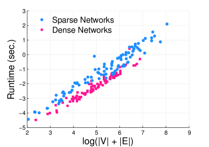
Figure 5: Scalability of the Proposed Coloring Methods. The x-axis represents the log of the size of the graph whereas the y-axis is the log runtime (in seconds). For both large sparse and dense networks, find that the proposed methods scale linearly as the size of the graph increases and thus practical for a variety of applications.

These results indicate that in practice, the proposed methods are fast, scaling linearly as the size of the graph increases. Hence, these methods are well-suited for use in a variety of applications including network analysis, relational machine learning, sampling, among many others. See Section 7.3 for details on the scalability of the neighborhood coloring methods.

Table 8: Recolor Statistics. We compare the variants that use recolor to those that do not. The statistics in the table are computed over all graphs and greedy coloring methods. The max and mean improvement are measured as the maximum/average difference between the number of colors used before and after recoloring.

	Percentage		Difference
	Improved	Same	Max Diff.	Mean Diff.
Sparse	40.9%	59.1%	11	1.01
Dense	84.4%	14.6%	313	14.65

6.3 Effectiveness of Recolor

This section investigates the effectiveness of the recolor method. In particular, how often does it reduce the number of colors? For this, we investigate and compare greedy coloring variants that utilize recolor to the methods that do not. Given a graph $G$ and a vertex ordering $\pi$ from one of the proposed selection strategies in Section 3.2, we color the graph using the basic coloring framework (Algorithm 1) and then we color the graph again using the recolor method. From these two colorings, we measure the difference in the number of colors (after recoloring and before recoloring) and number of times the recolor method improved over the basic method. The results are shown in Table 8. Note that the statistics are computed over all graphs and greedy coloring methods, including the methods that do not perform well (i.e., degree-based methods). Note that the maximum improvement (i.e, Max Diff. in Table 8) and average improvement (i.e, Mean Diff. in Table 8) are measured as the maximum/average difference between the number of colors used before and after recoloring.

In sparse graphs, the recolor method results in fewer colors $40.9\%$ of the time whereas the improvement for dense graphs is $84.4\%$. We find that the improvement for dense graphs is much larger since the number of colors initially (before recoloring) used on average is usually far from the optimal number. Note that for sparse graphs, this includes the graphs where the greedy coloring methods was able to find the optimal number of colors (and thus, it is impossible for recolor to improve over the basic coloring). Additionally, the sparse graphs use fewer colors than the dense graphs and also the number of colors used from the greedy coloring methods tends to be closer to the optimal. These results indicate that recolor is both fast and effective for reducing the number of colors used by any of the proposed methods.

In addition, we also provide results for both recolor and basic variants on a variety of large sparse real-world networks, see Table 9 and Table 10. These can be used to infer additional insights. In Table 18 and Table 19, we also compare the recolor variant to the faster but less accurate basic coloring variant of each coloring method for the DIMACs and BHOSLIB graph collections.

Table 9: Recolor variant is compared to the faster but less accurate basic variant for each of the proposed methods. We also include four previous methods for comparison. For each graph, the top row is the results from the basic variant whereas the bottom row is from the recolor variant.

Stats & Bounds								Coloring Methods
	graph	$|E|$	$\Delta$	$K$+1	$T$	$\tilde{\omega}$	rand	deg	ido	dist-two-ido	triangles	kcore-deg	triangle-vol	triangle-core-vol	triangle-core-max	deg-triangles	kcore-triangles	kcore-deg-tri	deg-kcore-vol	kcore-triangle-vol	deg-kcore-triangle-vol
	soc-BlogCat.	2M	9.4K	222	101	24	124	89	89	89	88	88	87	87	87	88	90	109	108	115	117
							118	85	85	85	83	84	84	84	84	85	85	102	102	110	112
	soc-LiveMo.	2.1M	2.9K	93	27	10	53	38	38	38	39	39	34	34	34	36	36	37	38	36	45
							50	36	36	36	36	36	30	30	30	33	33	36	37	33	42
	soc-buzznet	2.7M	64.2K	154	59	21	89	63	63	63	62	62	63	63	63	64	65	79	80	87	86
							85	59	59	59	59	58	59	59	59	59	58	74	75	82	83
	soc-delicious	1.3M	3.2K	34	23	17	26	22	22	22	22	22	22	22	22	21	21	21	21	21	22
							25	22	22	22	22	22	22	22	22	21	21	21	21	21	21
	soc-digg	5.9M	17.6K	237	73	41	93	66	66	66	67	67	71	71	71	64	64	81	82	89	90
							88	63	63	63	63	63	63	63	63	61	61	75	77	80	83
	soc-douban	327K	287	16	11	8	17	14	14	14	13	13	13	13	13	13	13	13	13	13	13
							17	14	14	14	13	13	13	13	13	13	13	13	13	13	12
	soc-epinions	100K	443	33	18	14	30	25	25	25	25	25	20	20	20	20	20	20	20	20	21
							28	22	22	22	22	22	20	20	20	20	20	20	20	20	20
	soc-flickr	3.1M	4.3K	310	153	21	146	109	109	109	108	108	104	104	104	105	106	129	126	138	142
							138	104	104	104	102	102	100	100	100	100	99	118	119	127	131
	soc-flixster	7.9M	1.4K	69	47	29	57	47	47	47	47	47	47	47	47	44	44	40	40	40	49
							53	46	46	46	46	46	46	46	46	42	42	38	38	38	46
	soc-gowalla	950K	14.7K	52	29	29	44	30	30	30	30	30	30	30	30	30	30	29	29	29	37
							42	30	30	30	29	29	29	29	29	29	29	29	29	29	37
	soc-lastfm	4.5M	5.1K	71	23	14	43	26	26	26	26	26	27	27	27	24	24	28	28	27	40
							39	26	26	26	26	26	25	25	25	23	23	28	28	27	36
	soc-pokec	22.3M	14.8K	48	29	29	43	33	33	33	33	33	33	33	33	33	33	30	30	30	38
							41	31	31	31	31	31	31	31	31	32	32	29	29	29	37
	soc-slashdot	358K	2.5K	54	35	17	44	39	39	39	40	40	34	34	34	35	35	35	35	35	43
							42	36	36	36	36	36	31	31	31	32	32	32	32	32	41
	soc-wiki-Vote	2.9K	102	10	7	7	11	9	9	9	9	9	8	8	8	8	8	7	7	8	8
							10	8	8	8	8	8	8	8	8	8	8	7	7	7	8
	soc-youtu-sn	2.9M	28.7K	52	19	13	44	33	33	33	33	33	33	33	33	31	31	30	30	31	40
							42	31	31	31	31	31	31	31	31	30	30	28	28	29	37
	soc-youtube	1.9M	25.4K	50	19	11	42	32	32	32	32	32	30	30	30	30	30	28	28	29	37
							40	29	29	29	30	30	29	29	29	28	28	27	27	28	36

Table 10: Recolor variant is compared to the faster but less accurate basic variant for each of the proposed methods (continued from Table 9). We also include four previous methods for comparison. For each graph, the top row is the results from the basic variant whereas the bottom row is from the recolor variant.

Stats & Bounds								Coloring Methods
	graph	$|E|$	$\Delta$	$K$+1	$T$	$\tilde{\omega}$	rand	deg	ido	dist-two-ido	triangles	kcore-deg	triangle-vol	triangle-core-vol	triangle-core-max	deg-triangles	kcore-triangles	kcore-deg-tri	deg-kcore-vol	kcore-triangle-vol	deg-kcore-triangle-vol
	ia-email-EU	54.3K	623	23	13	11	23	19	19	19	18	18	17	17	17	17	17	17	17	17	16
							22	17	17	17	18	18	17	17	17	16	16	16	16	16	15
	ia-enron-large	180K	1.3K	44	22	15	40	31	31	31	30	30	28	28	28	28	28	28	28	28	37
							38	29	29	29	29	29	26	26	26	27	27	27	27	28	34
	ia-fb-messages	6.4K	112	12	5	5	12	9	9	9	8	8	8	8	8	9	9	8	9	8	9
							12	9	9	9	8	8	8	8	8	8	8	8	9	9	9
	ia-wiki-Talk	360K	1.2K	59	20	9	45	35	35	35	34	34	30	30	30	31	31	31	31	31	40
							43	33	33	33	32	32	28	28	28	28	28	29	29	28	37
	fb-B-anon	20.9M	4.3K	64	31	23	47	30	30	30	30	30	30	30	30	29	29	29	29	30	41
	45						28	28	28	28	28	28	28	28	28	28	27	27	28	37
fb-Berkeley13	852K	3.4K	65	47	39	57	49	49	49	49	49	50	50	50	48	48	49	49	49	56
						55	47	47	47	49	49	48	48	48	47	47	46	46	46	52
fb-CMU	249K	840	70	45	42	58	50	50	50	50	50	49	49	49	51	51	50	50	51	55
						56	49	49	49	48	48	47	47	47	47	47	49	49	47	53
fb-Duke14	506K	1.8K	86	47	29	64	56	56	56	55	55	47	47	47	52	52	49	49	49	61
						61	50	50	50	50	50	45	45	45	46	46	47	47	47	54
fb-Indiana	1.3M	1.3K	77	53	43	66	58	58	58	58	58	56	56	56	54	54	54	54	52	62
						62	55	55	55	54	54	52	52	52	51	51	51	51	51	57
fb-MIT	251K	708	73	41	30	59	50	50	50	48	48	44	44	44	46	46	46	46	47	55
						57	47	47	47	44	44	43	43	43	43	43	44	44	43	50
fb-OR	816K	1K	53	36	28	46	41	41	41	41	41	37	37	37	37	37	37	37	36	44
						44	37	37	37	38	38	34	34	34	34	34	34	34	34	42
fb-Penn94	1.3M	4.4K	63	48	43	56	52	52	52	53	53	48	48	48	50	50	48	48	47	52
						53	49	49	49	49	49	47	47	47	46	46	46	46	46	51
fb-Stanford3	568K	1.1K	92	60	47	68	63	63	63	63	63	59	59	59	58	58	59	59	60	67
							64	58	58	58	58	58	55	55	55	55	55	55	55	56	61
	fb-Texas84	1.5M	6.3K	82	62	44	74	64	64	64	64	64	57	57	57	60	60	60	60	61	71
							71	62	62	62	61	61	56	56	56	57	57	57	57	56	65
	fb-UCSB37	482K	810	66	60	51	63	59	59	59	60	60	56	56	56	56	56	56	56	56	62
							62	56	56	56	57	58	55	55	55	55	55	55	55	54	59
	fb-UConn	604K	1.7K	66	53	47	60	56	56	56	57	57	56	56	56	51	51	52	52	52	57
							58	51	51	51	53	53	51	51	51	50	50	50	50	50	54
	fb-UF	1.4M	8.2K	84	67	51	75	66	66	66	65	65	64	64	64	61	61	62	62	61	72
							71	62	62	62	62	62	60	60	60	59	59	61	61	59	66
	fb-UIllinois	1.2M	4.6K	86	65	54	72	64	64	64	63	63	62	62	62	59	59	60	60	61	68
							68	60	60	60	61	61	58	58	58	58	58	58	58	58	64
	fb-Wisconsin87	835K	3.4K	61	42	34	54	48	48	48	47	47	46	46	46	44	44	43	43	42	51
							52	45	45	45	45	45	43	43	43	42	42	42	42	42	48
	tech-RL-caida	607K	1K	33	19	15	25	20	20	20	20	20	20	20	20	19	19	19	19	19	18
							24	19	19	19	19	19	19	19	19	19	19	18	18	17	18
	tech-WHOIS	56.9K	1K	89	71	49	72	67	67	67	67	66	67	67	67	66	66	67	67	66	72
							66	62	62	62	61	61	60	60	60	63	63	62	62	63	64
	tech-internet-as	85.1K	3.3K	24	17	14	22	19	19	19	19	19	19	19	19	19	19	18	18	19	20
							21	18	18	18	18	18	18	18	18	18	18	17	17	18	18
	tech-routers-rf	6.6K	109	16	16	16	18	17	17	17	16	16	17	17	17	17	17	16	16	17	17
							16	17	17	17	16	16	17	17	17	17	17	16	16	17	16

6.4 Bounds & Provably Optimal Coloring

This section describes two ways to leverage the bounds. Results are then provided in Table 3 and Table 4 for a representative set of graphs from the collection.

First, the lower bound can be used to verify that the coloring from a greedy method is optimal. Let $\tilde{\omega}(G)$ be a lower bound of $\chi(G)$ (i.e., optimal number of colors), then we have the following simple relationship:

$$\tilde{\omega}(G)\leq\omega(G)\leq\chi(G)\leq{\rm\chi}(G,\pi)\leq\Delta(G)+1$$

where ${\rm\chi}(G,\pi)$ is the number of colors from a greedy coloring that uses $\pi$ and $\Delta(G)+1$ is the maximum degree of $G$. Consequently, if $\tilde{\omega}(G)={\rm\chi}(G,\pi)$, then as a result of the above, we know ${\rm\chi}(G,\pi)$ must be optimal.

Second, we may also use the bounds to characterize the accuracy of a greedy coloring method or prove that a solution is not optimal. For instance, suppose ${\rm\tilde{\omega}(G)}\leq K(G)\leq{\rm\chi}(G,\pi)$, then we know ${\rm\chi}(G,\pi)$ is not optimal.

We find the optimal number of colors is directly obtained and verified via both lower and upper bounds for nearly all collaboration networks and web graphs as shown in Table 3. In 6 of the 13 collaboration networks, we found that $\tilde{\omega}(G)={\rm\chi}_{\min}(G,\pi)={\rm\chi}_{\max}(G,\pi)=K(G)+1=T(G)$ where ${\rm\chi}_{\min}(G,\pi)$ and ${\rm\chi}_{\max}(G,\pi)$ are the min and max number of colors used by any of the coloring methods. This implies that the ordering is insignificant for these networks as all the methods resulted in a coloring that is provably optimal. Notably, from the 7 other networks, 5 of them differ only in ${\rm\chi}_{\max}(G,\pi)$. In addition, many other interesting observations and insights may be drawn from Table 4 and Table 3.

To summarize we find that: (i) For some types of information networks, the proposed greedy coloring methods produce an optimal coloring. (ii) The upper and lower bounds are effective for proving the optimality or suboptimality of a solution from a greedy coloring heuristic. (iii) For the majority of graphs that are significantly skewed and power-lawed, the optimal number of colors is directly obtained and verified via both lower and upper bounds.

7 Finding Colorful Neighborhoods

Given a large graph or a collection of neighborhood subgraphs, how can we define a domain-independent basis that succinctly characterizes the common structural properties of the neighborhood subgraphs? For this task, we define the problem of coloring local neighborhood subgraphs and propose a fast parallel flexible approach for solving it. Formally, a neighborhood subgraph can be defined as the induced subgraph centered around a vertex $v$ and induced by all neighbors of $v$. Our parallel neighborhood coloring framework makes heavy use of the proposed coloring methods from Table 1 as well as the basic coloring variant in Alg 1 and the more accurate recolor variant shown in Alg 5. In particular, we propose parallel methods for coloring neighborhoods that are (i) fast and scalable for large networks, (ii) space-efficient, (iii) flexible for a variety of applications, (iv) and accurate, finding in many cases nearly optimal or provably optimal solutions.

One of the main observations we make is that neighborhoods that are colored using a relatively few number of colors are not well connected, with low clustering and a small number of triangles. To understand this fundamental finding and the key intuition, we provide a series of simple neighborhood colorings shown in Figure 6. We also observe that neighborhoods that are colored using a relatively large number of colors have large clustering coefficients and usually contain large cliques relative in size to the other neighborhood colorings. Therefore, the set of neighborhood colorings is an important fundamental graph property, giving a number of key insights into the structural properties of the network at large and its local neighborhoods. In a similar manner as we have demonstrated above, one can also use neighborhood coloring to draw a number of other interesting insights and ultimately use it for characterizing the structure and behavior of many types of large networks. Besides these key benefits, we demonstrate that neighborhood coloring is fast and scalable to compute for large networks, and more specifically, it is linear in the number of edges. This is clearly much faster than computing the frequency of vertex/edge triangles Rossi (2014) or counting the frequency of other subgraph patterns and motifs Pržulj (2007); Shervashidze et al (2009); Rahman et al (2012). We also show that it is straightforward to parallelize for both shared-memory (CPU and GPU) and distributed architectures.

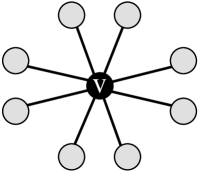
(a) Star

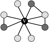
(b) Star w/ Triangles

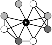
(c) Small Cliques

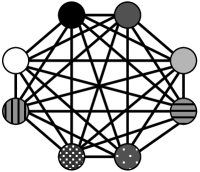
(d) Large Clique

Figure 6: Neighborhood Coloring Extremes: From Stars to Cliques. For (a)-(c), the vertex $v$ in the center is the vertex in which the neighborhood was induced, thus the other vertices are in the set $N(v)$. In (a) the vertex neighborhood is a simple star–no connections between the neighbors of $v$, and thus can be colored using only 2 colors. The neighborhood subgraph in (b) is essentially a star with a few neighbors of $v$ with edges among each other, thus, forming triangles. Similarly, in (c) we find more neighbors forming connections among each other giving rise numerous triangles and two cliques of size 4. Finally, the neighborhood subgraph in (d) represents a single large clique. Node $v$ was removed for clarity. These neighborhood subgraphs go from the least constrained neighborhood representing a star (a) to the most constrained neighborhood representing a clique (d). The neighborhood subgraphs shown in (b) and (c) are better representatives of neighborhood subgraphs found in large real-world networks (e.g., Facebook or other social networks). Note that in reality, the vertex $v$ in which the neighborhood subgraph corresponds may be removed from the coloring, since $v$ must be connected to every other vertex. Thus, the neighborhood subgraphs above are (k-1)-colorable when $v$ is removed.

Local neighborhood coloring consists of assigning a color to every vertex in a vertex neighborhood such that no two vertices linked by an edge share the same color while minimizing the number of colors used. The most colorful neighborhood is the one that requires the maximum number of colors. In this section, we propose parallel methods for coloring neighborhoods that are (i) fast and scalable for large networks, (ii) space-efficient, (iii) flexible for a variety of applications, (iv) and accurate, finding in many cases nearly optimal or provably optimal solutions.

The neighborhood colorings may be useful for finding better communities, especially in local community detection methods Malliaros et al (2012). Besides community methods, neighborhood coloring may also be used in prediction tasks such as detecting anomalous patterns in graphs, see Akoglu et al (2010) for one such egonet-based method. Other prediction tasks such as relational classification may also benefit from neighborhood coloring. For instance, one may construct a set of node features such as from these neighborhood colorings to improve the accuracy of classification (e.g., number of colors, largest independent set).

The results of our neighborhood coloring have direct and immediate implications on exact algorithms for the maximum clique problem Bomze et al (1999); Prosser (2012). In fact, the most successful approaches have used coloring as a bound, but vary in the ordering and method used Konc and Janezic (2007); San Segundo et al (2011); Tomita and Kameda (2007); Tomita et al (2011, 2010); Rossi et al (2012). For instance, suppose vertex neighborhoods are searched in parallel, similar to our heuristic in Alg 6, then the neighborhood coloring results may be used for bounding the search space in branch-n-bound algorithms, for pruning entire neighborhoods directly, and for ordering vertices via the number of colors from the vertex neighborhood coloring, among many other vertex level features that could be derived from such a set of neighborhood colorings. These may enhance recent parallel algorithms such as pmc Rossi et al (2014) that utilizes degeneracy ordering giving a worst-case runtime of $O(2^{d/4})$ on sparse graphs with bounded degeneracy. In addition, super-linear speedups may become more frequent using the ordering from neighborhood coloring/pruning, i.e., these were observed using pmc Rossi et al (2014) and later confirmed again using a parallel version of mcs Tomita et al (2010); McCreesh and Prosser (2013). Nevertheless, the set of vertex neighborhood colorings may also be used for pruning in other ego-centric search methods. They also provide a basis for a variety of ordering methods which may have applications, e.g., graph compression Boldi and Vigna (2004).

7.1 Problem Formulation

Our focus is on coloring vertex neighborhoods. Let $N(v)=\{v\}\cup\{u:(u,v)\in E\}$ be the closed neighborhood of a vertex $v$ and we define $H_{v}$ as the neighborhood subgraph induced from $N(v)$, consisting of $v$, the neighbors of $v$, and any edges between them. Suppose $H_{v}$ is a neighborhood subgraph of $G$ and $G$ is $k$-colorable, then $H_{v}$ must also be $k$-colorable. Consequently, if $H_{v}$ is a subgraph of $G$, then $\chi(H)\leq\chi(G)$.

The local chromatic number of $G$ is the maximum number of colors appearing in the closed neighborhood (subgraph) of a vertex minimized over all proper colorings. More formally,

$${\rm\chi_{\ell}}(G)=\min_{c}\;\;\max_{v\in V}\;|\{c(u):u\in N(v)\}|$$

where the minimum is taken over all proper colorings $c$ and ${\rm\chi_{\ell}}(G)$ is the number of colors appearing in the most colorful closed neighborhood of a vertex. Clearly, ${\rm\chi_{\ell}}(G)\leq\chi(G)$ and we find for large real-world graphs (i.e., social and information networks Mislove et al (2007); Ahmed et al (2013)) these two numbers are usually close. Despite this result, we note that for general graphs ${\rm\chi_{\ell}}(G)$ may be small while $\chi(G)$ can be arbitrarily large Erdös et al (1986); Godsil et al (2001).

We relax the strict requirement above from considering all proper colorings to considering only a single proper coloring for each neighborhood. In particular, this article proposes a framework of local greedy coloring methods designed for dense and large sparse graphs found in real-world (e.g., social networks). Given a neighborhood subgraph of $v$ denoted $H_{v}$ and a graph property $f(\cdot)$, let $f(H_{v})=\bm{\mathrm{x}}$ where $\bm{\mathrm{x}}\in\mathbb{R}^{n}$ is a vector of vertex weights and $x_{i}$ is the value of vertex $u_{i}\in N(v)$. Using the weight vector $\bm{\mathrm{x}}$ as a basis for ordering the vertices in the closed neighborhood, we denote this ordering as $\pi_{v}=\{u_{1},u_{2},...\}$. Further, let ${\rm\chi}({H},\pi_{v})$ be the number of colors used by a local greedy coloring algorithm that uses the ordering $\pi_{v}$ to color ${H}$. Consequently, an approximation of the local chromatic number of $G$ is defined as:

$${\rm\chi_{\ell}}(G,\Pi)=\max_{v\in V}\;{\rm\chi}(N[v],\pi_{v})$$

where ${\rm\chi_{\ell}}(G,\Pi)$ is the maximum number of colors used by a local greedy coloring method that uses the set of neighborhood vertex orderings $\Pi=\{\pi_{v_{1}},\pi_{v_{2}},...,\pi_{v_{n}}\}$. Intuitively, the above gives rise to the following relationship:

$$\omega(G)\leq\chi(G)\leq{\rm\chi_{\ell}}(G,\Pi)$$

Also, if we consider a vertex neighborhood subgraph ${H}_{v}$, then:

$$\omega({H}_{v})\leq\chi({H}_{v})\leq{\rm\chi}({H}_{v},\pi_{v})\leq\Delta({H}_{v})+1$$

where $\omega({H}_{v})$ is the size of the maximum clique, $\chi({H}_{v})$ is the optimal number of colors required to color ${H}_{v}$ (minimized over all proper colorings of $N(v)$), and ${\rm\chi}({H}_{v},\pi_{v})$ is the number of colors from a greedy coloring of $N(v)$ using $\pi_{v}\in\Pi$.

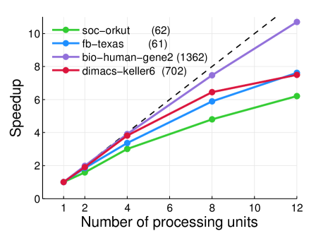
(a) Representative Graphs

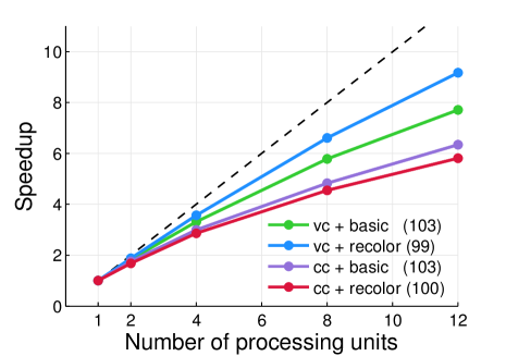
(b) Coloring Variants

Figure 7: Scalability. The speedup of our methods on different types of graphs are shown in Fig. 7(a), whereas the speedup of different coloring variants for soc-flickr are shown in Fig. 7(b). It is clear that all proposed variants are scalable for large graphs, while vertex-centric coloring (vc) using recolor scales slightly better than the others for the large sparse flickr social network. Processing units are cores (one thread per core).

7.2 Neighborhood Coloring

The parallel framework is shown in Alg 7. Here, $B(\cdot)$ is assumed to be normalized with respect to cliques, hence, $B(v)=K(v)+1$. This allows us to generalize the algorithm over any arbitrary upper bound.

Algorithm 7 Parallel Neighborhood Coloring Framework

1Initialize data structures

2Compute upper bounds $B(G)$

3Obtain a lower bound $\omega(G)\leftarrow\textsc{HeuClique}(G)$

4Prune vertices and edges from $G$ (explicitly)

5Obtain a vertex ordering $\pi=\{v_{1},...,v_{n}\}$

6for each $v_{i}$ in an ordering $\pi$ in parallel  do

7    if $B(v_{i})>{\mathtt{max}}$ then

8        $P\leftarrow\{v_{i}\}$

9        for $w\in N(v_{i})$ do

10           if $B(w)>{\mathtt{max}}$ then $P\leftarrow P\cup\{w\}$                    

11        Set $\bm{\mathrm{x}}$ to be the computed graph property $f(P)$

12        Order vertices in $P$ using $\bm{\mathrm{x}}$

13        $k\leftarrow$ ColoringVariant($G$, $P$)

14        if $k>{\mathtt{max}}$ then ${\mathtt{max}}\leftarrow k$              

15return ${\rm\chi_{\ell}}(G,\pi)\leftarrow{\mathtt{max}}$

Upper and lower bounds are computed in Line 2 and 3, respectively, and used for pruning in Line 4. The vertices remaining in $G$ are ordered in Line 5, and then each vertex neighborhood in that order are colored (Line 6). For each vertex in order, we first try to avoid coloring $v_{i}$ by checking if the local vertex upper bound $B(v_{i})$ is smaller than ${\mathtt{max}}$. If not, then lines 8–10 form the ”reduced” set $P$ of neighboring vertices. In line 12, we obtain the local vertex ordering $\pi_{v_{i}}$ by ordering the vertices in $P$ using an arbitrary property $f(P)$ computed in line 11. Next, the subgraph $H_{v}$ induced by the ordered vertex set $P$ are colored using a coloring variant and color assignment/search strategy (Line 13). Finally, line 14 updates the maximum number of neighborhood colors required, if necessary.

Note that the three pruning steps are shown in Line 4, 7, and Line 10, respectively. If the goal is to compute ${\rm\chi_{\ell}}(G,\pi)$, then the pruning steps can significantly reduce the search space leading to faster and more accurate colorings. For the problem of computing the complete set of neighborhood colorings, then we can simply avoid using the pruning steps. In other words, the pruning steps and their utility are application dependent, and thus may be turned on/off accordingly. We also note that these pruning steps are also useful for finding the max clique, computing a graph property for which the upper and lower bounds apply, and for finding dense subgraphs, among many other tasks.

In addition to the coloring variants from Section 3 and 4, we also investigate two types of search procedures for coloring (i.e., color-centric and vertex-centric) that differ in their implementation, but may result in significantly different runtimes depending on the structural properties of the input graph. In particular, the search procedure in the basic and recolor variants may be performed by searching color-classes (i.e., the independent sets) or by searching the vertex neighborhoods (i.e., adjacent vertices) and thus, we term these search procedures as color-centric and vertex-centric, respectively.

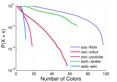
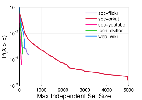
Figure 8: Properties of the Neighborhood Colorings. Using the parallel neighborhood coloring algorithm, we color each vertex-induced neighborhood and record the number of colors used for that neighborhood as well as the maximum independent set size (i.e., largest such coloring class given by the neighborhood coloring of that vertex). We use the complementary cumulative distribution function (CCDF) to study the coloring properties of a few large sparse real-world networks. The max independent set size is with respect to the coloring (largest such coloring class).

7.2.1 Parallelization

The neighborhood coloring problem is parallelized by considering each neighborhood subgraph as independent and coloring each of these subgraphs in parallel. We use dynamic scheduling and assign each processing unit a single neighborhood at a time. This helps ensure the vertex neighborhoods are colored in approximately the correct order. Our approach requires a single lock to ensure that the largest number of colors used thus far is consistent and avoid potential race conditions when updating it (see line 14). Importantly, as soon as a processing unit updates ${\mathtt{max}}$, we immediately broadcast it to all other processing units. We observed that this can significantly improve performance as the tighter lower bound may be used for additional pruning or result in terminating a search early. As an aside, if the pruning rules are used, then two subsequent runs may result in slightly different ${\rm\chi_{\ell}}(G,\pi)$. This is due to possible variations in the global vertex ordering which determines the underlying order in which the neighborhoods are colored.

The parallel framework has many other advantages. For instance, each processing unit only requires a neighborhood subgraph and therefore the framework is space efficient for streaming or graphs too large to reside in memory and thus a good candidate for GPU parallelization as well.

Table 11: Upper and Lower Bounds of the Chromatic Number for the Graphs. We denote ${\rm\chi}(G,\pi)$ as the maximum number of colors used from the set of neighborhood colorings. Note that ${\rm\chi}(G,\pi)$ is computed using none of the pruning steps and thus is larger than if pruning is used.

	Graph stats							Bounds
graph	$|V|$	$|E|$	$|T|$	$\bar{d}$	${\rm r}$	$\kappa$	${\rm tr}_{\rm max}$	$\Delta$	$K$+1	$T$	$\tilde{\omega}$	${\rm\chi}(G,\pi)$
soc-flickr	513K	3.1M	176M	12	0.16	0.15	524K	4.3K	310	153	21	104
soc-orkut	2.9M	106M	1.5B	70	0.02	0.04	1.3M	27.4K	231	75	37	83
soc-youtube	495K	1.9M	7.3M	7	-0.03	0.01	151K	25.4K	50	19	11	28
tech-as-skitter	1.6M	11M	86.3M	13	-0.08	0.01	564K	35.4K	112	68	41	70
bio-human-gene2	14K	9M	14.7B	1.2K	0.8	0.59	6.9M	7.2K	1903	1681	1267	1329
keller6	3.3K	4.6M	10.3B	2.7K	-0.02	0.82	3.5M	2.9K	2691	2084	45	148

7.3 Experiments

We now analyze the effectiveness of our approach on a variety of real-world networks. The network statistics including lower and upper bounds are provided in Figure 11.

A number of observations are made from the experiments. First and foremost, the scalability of our parallel framework is demonstrated in Figure 7 where we observe that significant speedups are possible across a range of different types of graphs and coloring variants. Importantly, Fig. 7(a) demonstrates the scalability of our methods on a diverse set of graphs, from large sparse graphs (e.g., social and biological networks) to dense networks found in scientific computing. Besides density, these graphs are known to contain very different structural properties. We used the large Orkut social network that is sparse and power-lawed, the sparse Facebook Texas network, a slightly more dense biological network of a human gene, and a very dense unsolved instance from the clique/coloring DIMAC’s challenge. The last two graphs were found to be more difficult to obtain nearly optimal local colorings. Nevertheless, these two graphs, but especially the human gene, scale slightly stronger than the more sparse networks. These graphs were colored using the basic coloring method with color-centric search and no pruning. Further, vertices were ordered globally by kcore-vol ($f(v)=\sum_{w\in N(v)}K(w)$) and ordered locally using kcore-deg-vol and both orderings are from largest to smallest for simplicity.

Finally, we also investigated the scalability of a few different coloring variants using the large sparse flickr social network, see Figure 7(b) for details. In particular, all the proposed variants are shown to scale well for large graphs, while vertex-centric coloring (vc) using recolor scales slightly better than the others. Similar results were also observed using other types of graphs and methods.

Table 12: Comparing the Space of Neighborhood Coloring Methods. We evaluate a representative set of methods from the framework. The local coloring number denoted ${\rm\chi_{\ell}}(G,\pi)$ is given for each of the variations. We present results for a representative sample of methods from the framework. In all methods, the local ordering is from largest to smallest, whereas the global ordering is from smallest to largest. For the global ordering we used kcore-vol for simplicity, while varying the local ordering method.

		Ordering Techniques
Variant	Pruning	Rand	Kcore	Triangle	Tcore	Kcore-vol	Tri-vol	Tcore-vol	Deg-Kcore-vol
Basic	✓	60	58	54	58	54	54	58	54
	✗	68	62	58	62	57	57	62	56
Recolor	✓	57	57	53	57	53	52	57	52
	✗	67	61	56	61	57	56	61	56

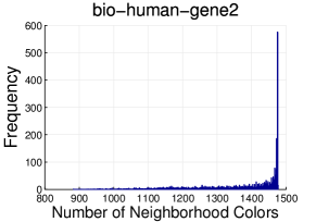
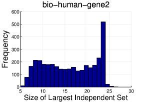
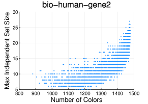
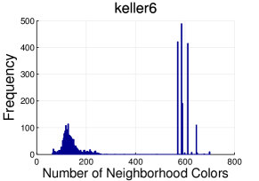
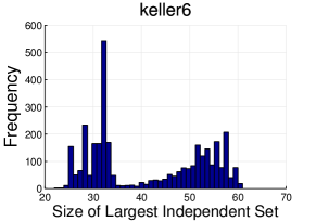
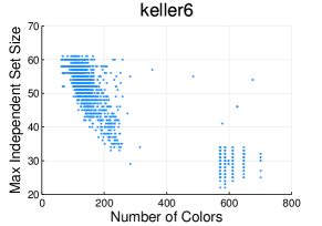
Figure 9: Characterizing and comparing the various types of networks using statistics from neighborhood coloring. The number of colors used to color each of the neighborhoods are shown along with the size of the largest independent set in the coloring of the neighborhoods.

Now, we investigate a representative sample of coloring methods from the large space defined by the framework. For this experiment, we use the three pruning steps and order the vertices globally using kcore-vol and are searched from smallest to largest. The vertices in each neighborhood are ordered from maximum to minimum and thus the vertices more constrained in their choice of color are assigned colors early allowing more flexibility in the color assignment whereas vertices that are not as constrained take lower precedence in their color assignment since these vertices are usually easily assigned to a color. In both global and local ordering, ties are broken using vertex ids such that if $f(v)=f(u)$ and $v>u$, then $v$ is ordered before $u$.

The results from a single graph (soc-flickr) are shown in Table 12, others were removed for brevity. The first row represents the family of methods that use the basic variant with pruning, whereas the second row uses no pruning. Likewise, the third and fourth rows use recolor with pruning and without it, respectively. There are several interesting observations. First, the coloring number from the recolor variant is at least as accurate and usually better than the basic variant. This result is independent of whether pruning is used or not and it shows how much improvement can be achieved by using the recolor variant. Second, pruning is generally effective in obtaining a better coloring number. Note that using both pruning and the recolor variant clearly improves on the basic coloring method (without pruning or recolor). For example, using the Tri-vol method, we get a $\approx 9\%$ improvement in the number of colors, when we apply both pruning and recolor variant. Finally, we observe that the Tri-vol and Deg-Kcore-vol methods perform the best among all other methods (minimum number of colors). These results are consistent with the pervious discussion in Section 6.

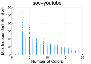
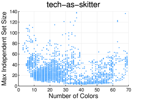
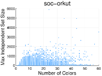
Figure 10: Exploring the relationship between two statistics from the neighborhood coloring. The number of colors used in each local coloring is compared with the size of the largest independent set from that coloring.

In this section, we use neighborhood coloring to characterize the various types of networks as well as gain insight into the structural properties of the networks. We view the neighborhood coloring as a process for discovering meaningful features that capture some underlying properties of the graph that arise from the notion of coloring. From this, we first derive two vertex features. Specifically, for each vertex $v$, the first feature represents the number of colors used in the neighborhood coloring of the vertex $v$, and the second feature represents the size of the maximum independent set resulting from the neighborhood coloring of the vertex $v$. Figure 8 shows the complementary cumulative distribution (CCDF) of these features across all the nodes in the graph. We observe that those graphs that are denser and more clustered (such as soc-flickr) typically use many colors for neighborhood coloring of the vertices. For example, the soc-flickr dataset uses $100$ colors to color the largest vertex neighborhood in the graph. On the other hand, graphs that are more sparse and less clustered (such as soc-youtube) typically use fewer colors for neighborhood coloring of the vertices. Further, we observe that the maximum independent set size is inversely proportional to the maximum number of neighborhood colors. Clearly, this observation is due to the rate of dependence among the graph vertices. For example, the soc-flickr dataset has a small independent set size $\approx 400$ vertices. On the other hand, a graph that is as large and as sparse as soc-orkut typically has a large independent set size $\approx 5000$ vertices. These observations show how significant the two features (number of colors and maximum independent set size) for capturing the underlying structural properties of various types of graphs. Note that in Figure 8, we show only some of the datasets as examples, and we omit the others for brevity.

As an aside, egonet-based clique methods were proposed for sparse graphs Rossi et al (2012) and sampling methods and estimators based on egonets were developed in the same spirit Gjoka et al (2013); Ahmed et al (2013). One may also straightforwardly use egonets to obtain an accurate estimate of the distribution of local coloring numbers.

In Figure 9, we focus the attention on the other denser graphs, bio-human-gene2 and keller6. Figure 9 shows the histograms of the number of colors, maximum independent set size, and the correlation between them, for both bio-human-gene2 and keller6 graphs. We observe that the histograms of the number of colors and maximum independent set size are highly skewed. For example, bio-human-gene2 graph shows that $600$ vertices uses more than $1400$ colors for their neighborhood. Moreover, the size of the maximum independent set size has a small range ($5$-$25$). The keller6 graph, however, is one of the clique DIMAC’s challenge graphs. We observe that the histogram of the keller6 graph consists of two groups, one group with small number of colors ($<200$), and the other group with higher number ($\approx 600$) of colors. This observation is clearly shown in the histogram of the maximum independent set size. Similarly, we show the correlation plots between the number of colors and the maximum independent set size for several datasets in Figure 10. The observations are similar to what we discussed before.

8 Conclusion

Despite the obvious practical importance of graph coloring, existing works have not systematically investigated or designed methods for large complex networks. In this work, we defined a unified framework that can serve as a fundamental basis for studying coloring on large networks. Using this framework, we proposed three classes of fast and accurate methods including social-based, multi-property based, and egonet-based methods. We demonstrated the effectiveness of the proposed methods on over 100+ networks and among 7 different types of networks (e.g., social, technological networks). In the majority of cases, we found these methods to be more accurate than other widely used heuristics that have been used for coloring in other domains. Importantly, we find that the solutions obtained from our methods are nearly optimal and sometimes provably optimal for certain types of networks. Furthermore, the coloring methods were shown to be effective for the task of finding graph outliers as well as predicting the type of graph (e.g., social vs. biological network). We also investigated the problem of coloring neighborhood subgraphs and proposed a parallel algorithm that leverages the proposed unified framework and methods. One key finding is that neighborhoods that are colored using a relatively few number of colors are not well connected, with low clustering and a small number of triangles. While neighborhood colorings that use a relatively large number of colors have large clustering coefficients and usually contain large cliques. In future work, we plan to explore the neighborhood coloring further as it has proven to provide a number of key insights into the structural properties of the network and neighborhoods at large, while also fast to compute for large networks. Overall, this work demonstrated the practical significance, accuracy, and scalability of our methods for coloring and analyzing large complex networks.

Appendix

Table 13: Network Statistics and Coloring Bounds for DIMACs. Recall $\rho$ is the density, $\bar{d}$ is the average degree, and ${\rm r}$ is the assortativity coefficient. The global clustering coefficient is denoted by $\kappa$, $|T|$ is the total number of triangles, and $tr_{\rm avg}$ and $tr_{\rm\max}$ are the maximum and average number of triangles incident on a vertex, respectively. The lower bound from the heuristic clique finder is denoted $\tilde{\omega}$. For the upper bounds, we denote $K$ as the maximum k-core and similarly, we denote the maximum triangle-core by $T$. The maximum and minimum number of colors among all coloring methods are denoted ${\rm\chi}_{\max}$ and ${\rm\chi}_{\min}$, respectively.

	Graph measures						Bounds				Colors
graph	$|V|$	$|E|$	$|T|$	$\bar{d}$	$\kappa$	${\rm tr}_{\rm max}$	$\Delta$	$K$+1	$T$	$\tilde{\omega}$	${\rm\chi}_{\min}$	${\rm\chi}_{\max}$
C1000-9	1K	450K	364.6M	900	0.90	385K	925	875	764	51	311	327
C125-9	125	6.9K	691.8K	111	0.90	6.3K	119	103	86	27	54	59
C2000-5	2K	999.8K	499.7M	999	0.50	287.8K	1K	941	435	14	217	231
C2000-9	2K	1.7M	2.9T	1.7K	0.90	1.5M	1.8K	1759	1549	59	570	603
C250-9	250	27.9K	5.6M	223	0.90	24.8K	236	211	181	36	92	103
C4000-5	4K	4M	4T	2K	0.50	1.1M	2.1K	1910	899	15	391	408
C500-9	500	112.3K	45.3M	449	0.90	98.4K	468	433	373	44	168	183
DSJC1000-5	1K	249.8K	62.3M	499	0.50	75.9K	551	460	207	13	120	130
DSJC500-5	500	62.6K	7.8M	250	0.50	20.5K	286	226	99	11	67	75
MANN-a27	378	70.5K	26M	373	0.99	69K	374	365	352	125	138	144
MANN-a45	1K	533.1K	546.6M	1K	1.00	529K	1K	1013	991	341	367	375
MANN-a81	3.3K	5.5M	18.2T	3.3K	1.00	5.4M	3.3K	3281	3241	1096	1134	1161
MANN-a9	45	918	33.7K	40	0.92	757	41	41	37	16	19	21
brock200-1	200	14.8K	1.6M	148	0.75	10.1K	165	135	91	17	54	59
brock200-2	200	9.8K	479.6K	98	0.49	3.1K	114	85	35	9	33	37
brock200-3	200	12K	873.3K	120	0.61	5.4K	134	106	56	12	41	46
brock200-4	200	13K	1.1M	130	0.66	7K	147	118	68	14	44	52
brock400-1	400	59.7K	13.3M	298	0.75	38.1K	320	278	192	20	96	107
brock400-2	400	59.7K	13.3M	298	0.75	40.1K	328	279	193	20	97	104
brock400-3	400	59.6K	13.2M	298	0.75	38.5K	322	279	192	20	95	105
brock400-4	400	59.7K	13.3M	298	0.75	39.6K	326	278	193	22	95	107
brock800-1	800	207.5K	69.7M	518	0.65	101.4K	560	488	292	17	139	149
brock800-2	800	208.1K	70.4M	520	0.65	104K	566	487	292	18	139	150
brock800-3	800	207.3K	69.6M	518	0.65	100.8K	558	484	289	17	138	148
brock800-4	800	207.6K	69.9M	519	0.65	103.2K	565	486	291	17	141	146
c-fat200-1	200	1.5K	16.2K	15	0.73	100	17	15	12	12	13	16
c-fat200-2	200	3.2K	76.7K	32	0.76	429	34	33	24	24	24	28
c-fat200-5	200	8.4K	546.2K	84	0.77	2.8K	86	84	58	58	69	85
c-fat500-1	500	4.4K	55.7K	17	0.74	141	20	18	14	14	14	18
c-fat500-10	500	46.6K	6.6M	186	0.77	13.6K	188	186	126	126	126	188
c-fat500-2	500	9.1K	247K	36	0.76	534	38	36	26	26	26	33
c-fat500-5	500	23.1K	1.6M	92	0.77	3.4K	95	93	64	64	64	79
gen200-p0-9-44	200	17.9K	2.8M	179	0.90	16.1K	190	168	141	34	65	81
gen200-p0-9-55	200	17.9K	2.8M	179	0.90	16.1K	190	167	142	34	72	83
gen400-p0-9-55	400	71.8K	23.1M	359	0.90	63.1K	375	337	287	41	120	147
gen400-p0-9-65	400	71.8K	23.1M	359	0.90	64.1K	378	337	286	41	129	150
gen400-p0-9-75	400	71.8K	23.1M	359	0.90	64.8K	380	337	287	45	125	154
hamming10-2	1K	518.6K	519.7M	1K	0.99	507.5K	1K	1014	1004	512	512	540
hamming10-4	1K	434.1K	301.8M	848	0.82	294.7K	848	849	674	32	105	128
hamming6-2	64	1.8K	92.1K	57	0.90	1.4K	57	58	52	32	32	35
hamming6-4	64	704	2.8K	22	0.19	45	22	23	8	4	8	9
hamming8-2	256	31.6K	7.5M	247	0.97	29.4K	247	248	240	128	128	138
hamming8-4	256	20.8K	2M	163	0.60	7.8K	163	164	82	16	29	33

Table 14: Statistics and Bounds for DIMACs (cont. from Table 13). Recall $\rho$ is the density, $\bar{d}$ is the average degree, and ${\rm r}$ is the assortativity coefficient. The global clustering coefficient is denoted by $\kappa$, $|T|$ is the total number of triangles, and $tr_{\rm avg}$ and $tr_{\rm\max}$ are the maximum and average number of triangles incident on a vertex, respectively. The lower bound from the heuristic clique finder is denoted $\tilde{\omega}$. For the upper bounds, we denote $K$ as the maximum k-core and similarly, we denote the maximum triangle-core by $T$. The maximum and minimum number of colors among all coloring methods are denoted ${\rm\chi}_{\max}$ and ${\rm\chi}_{\min}$, respectively.

	Graph measures						Bounds				Colors
graph	$|V|$	$|E|$	$|T|$	$\bar{d}$	$\kappa$	${\rm tr}_{\rm max}$	$\Delta$	$K$+1	$T$	$\tilde{\omega}$	${\rm\chi}_{\min}$	${\rm\chi}_{\max}$
johnson16-2-4	120	5.4K	360.3K	91	0.73	3K	91	92	68	8	14	15
johnson32-2-4	496	107.8K	40.7M	435	0.87	82.2K	435	436	380	16	30	34
johnson8-2-4	28	210	1.2K	15	0.43	45	15	16	8	4	6	7
johnson8-4-4	70	1.8K	71.8K	53	0.74	1K	53	54	38	14	19	22
keller4	171	9.4K	649.7K	110	0.63	4.7K	124	103	54	9	24	37
keller5	776	225.9K	98M	582	0.75	151.2K	638	561	379	22	61	176
keller6	3.3K	4.6M	10.3T	2.7K	0.82	3.5M	2.9K	2691	2084	45	148	783
ph1000-1	1K	122.2K	9.2M	244	0.28	22.6K	408	164	47	9	55	78
ph1000-2	1K	244.7K	73.9M	489	0.57	157.6K	766	328	196	33	116	181
ph1000-3	1K	371.7K	211.3M	743	0.76	301.7K	895	610	388	49	194	269
ph1500-1	1.5K	284.9K	34.3M	379	0.29	53.2K	614	253	75	10	78	110
ph1500-2	1.5K	568.9K	273.5M	758	0.58	372.3K	1.1K	505	314	44	167	266
ph1500-3	1.5K	847.2K	741.1M	1.1K	0.77	675.7K	1.3K	930	597	60	281	388
ph300-3	300	33.3K	5.6M	222	0.76	26.7K	267	181	118	26	73	94
ph500-1	500	31.5K	1.2M	126	0.29	5.7K	204	87	25	9	34	48
ph500-2	500	62.9K	9.9M	251	0.58	40.8K	389	171	102	32	68	104
ph500-3	500	93.8K	27.1M	375	0.77	77.2K	452	304	197	39	111	150
ph700-1	700	60.9K	3.3M	174	0.29	11.5K	286	118	34	8	42	60
ph700-2	700	121.7K	26.6M	347	0.58	79.2K	539	236	143	26	91	141
ph700-3	700	183K	73.6M	522	0.76	147.9K	627	427	273	40	145	201
s1000	1K	250.5K	86.3M	501	0.69	100.7K	550	465	399	10	15	46
s200-0-7-1	200	13.9K	1.4M	139	0.73	8.5K	155	126	93	16	35	52
s200-0-7-2	200	13.9K	1.4M	139	0.74	9.7K	164	123	112	14	18	40
s200-0-9-1	200	17.9K	2.8M	179	0.90	16.3K	191	163	134	49	71	97
s200-0-9-2	200	17.9K	2.8M	179	0.90	15.8K	188	170	143	34	76	89
s200-0-9-3	200	17.9K	2.8M	179	0.90	15.6K	187	170	145	31	69	80
s400-0-5-1	400	39.9K	5.2M	199	0.66	15.8K	225	184	154	8	13	29
s400-0-7-1	400	55.8K	11.3M	279	0.73	32.3K	301	262	182	22	71	82
s400-0-7-2	400	55.8K	11.2M	279	0.73	32.8K	304	260	179	18	51	71
s400-0-7-3	400	55.8K	11.1M	279	0.72	33.6K	307	254	182	16	22	63
s400-0-9-1	400	71.8K	23.1M	359	0.90	62.7K	374	345	294	57	151	168
sr200-0-7	200	13.8K	1.3M	138	0.70	8.8K	161	125	78	16	48	55
sr200-0-9	200	17.8K	2.8M	178	0.90	15.9K	189	167	141	34	76	85
sr400-0-5	400	39.9K	3.9M	199	0.50	13.5K	233	178	77	10	56	64
sr400-0-7	400	55.8K	10.9M	279	0.70	33.5K	310	259	164	17	86	94

Table 15: Statistics and Bounds for BHOSLIB. Recall $\rho$ is the density, $\bar{d}$ is the average degree, and ${\rm r}$ is the assortativity coefficient. The global clustering coefficient is denoted by $\kappa$, $|T|$ is the total number of triangles, and $tr_{\rm avg}$ and $tr_{\rm\max}$ are the maximum and average number of triangles incident on a vertex, respectively. The lower bound from the heuristic clique finder is denoted $\tilde{\omega}$. For the upper bounds, we denote $K$ as the maximum k-core and similarly, we denote the maximum triangle-core by $T$. The maximum and minimum number of colors among all coloring methods are denoted ${\rm\chi}_{\max}$ and ${\rm\chi}_{\min}$, respectively.

	Graph measures						Bounds				Colors
graph	$|V|$	$|E|$	$|T|$	$\bar{d}$	$\kappa$	${\rm tr}_{\rm max}$	$\Delta$	$K$+1	$T$	$\tilde{\omega}$	${\rm\chi}_{\min}$	${\rm\chi}_{\max}$
frb100-40	4K	7.4M	25.5T	3.7K	0.93	6.9M	3.8K	3572	3468	78	106	558
frb30-15-1	450	83.1K	25.2M	369	0.82	67.4K	407	340	257	25	41	90
frb30-15-2	450	83.1K	25.1M	369	0.82	66.7K	404	338	257	24	36	93
frb30-15-3	450	83.2K	25.2M	369	0.82	65.2K	400	337	254	25	38	95
frb30-15-4	450	83.1K	25.2M	369	0.82	65.7K	401	340	255	25	36	94
frb30-15-5	450	83.2K	25.2M	369	0.82	66.4K	403	333	254	24	34	87
frb35-17-1	595	148.8K	62.5M	500	0.84	123.9K	544	463	361	29	41	118
frb35-17-2	595	148.8K	62.5M	500	0.84	122.2K	541	465	362	28	41	113
frb35-17-3	595	148.7K	62.5M	500	0.84	126.2K	549	451	352	28	38	113
frb35-17-4	595	148.8K	62.6M	500	0.84	131.1K	560	456	354	30	41	118
frb35-17-5	595	148.5K	62.2M	499	0.84	126.3K	550	461	355	29	45	115
frb40-19-1	760	247.1K	137.5M	650	0.86	210.6K	703	595	465	32	45	136
frb40-19-2	760	247.1K	137.5M	650	0.86	209.9K	702	598	477	33	45	145
frb40-19-3	760	247.3K	137.6M	650	0.86	210.2K	702	613	491	31	41	141
frb40-19-4	760	246.8K	136.8M	649	0.85	203.9K	692	600	481	32	50	144
frb40-19-5	760	246.8K	136.8M	649	0.85	203.6K	691	596	476	32	43	143
frb45-21-1	945	386.8K	274.2M	818	0.87	331.5K	876	769	626	36	51	187
frb45-21-2	945	387.4K	275.3M	819	0.87	326.9K	870	769	625	34	48	174
frb45-21-3	945	387.7K	276.2M	820	0.87	329.6K	872	764	624	35	48	182
frb45-21-4	945	387.4K	275.7M	820	0.87	331.2K	875	757	618	35	50	170
frb45-21-5	945	387.4K	275.4M	820	0.87	330.5K	874	771	629	37	49	175
frb50-23-1	1.1K	580.6K	514.4M	1K	0.88	496.1K	1K	950	786	39	52	202
frb50-23-2	1.1K	579.8K	512.4M	1K	0.88	504.6K	1K	936	771	39	53	204
frb50-23-3	1.1K	579.6K	511.5M	1K	0.88	508K	1K	953	792	40	55	210
frb50-23-4	1.1K	580.4K	513.9M	1K	0.88	502.6K	1K	950	786	40	58	196
frb50-23-5	1.1K	580.6K	514.6M	1K	0.88	510.8K	1K	949	790	41	56	200
frb53-24-1	1.2K	714.1K	707.5M	1.1K	0.88	619.3K	1.1K	1054	881	43	58	220
frb53-24-2	1.2K	714K	707.1M	1.1K	0.88	615.3K	1.1K	1057	884	43	57	228
frb53-24-3	1.2K	714.2K	707.7M	1.1K	0.88	616.5K	1.1K	1050	878	42	61	216
frb53-24-4	1.2K	714K	707M	1.1K	0.88	622.1K	1.1K	1063	890	43	59	217
frb53-24-5	1.2K	714.1K	707.2M	1.1K	0.88	633K	1.1K	1071	900	42	58	217
frb59-26-1	1.5K	1M	1.2T	1.3K	0.89	921K	1.4K	1282	1084	48	63	255
frb59-26-2	1.5K	1M	1.2T	1.3K	0.89	914.6K	1.4K	1285	1086	46	61	247
frb59-26-3	1.5K	1M	1.2T	1.3K	0.89	942.7K	1.4K	1296	1098	45	64	256
frb59-26-4	1.5K	1M	1.2T	1.3K	0.89	916.6K	1.4K	1284	1085	48	61	259
frb59-26-5	1.5K	1M	1.2T	1.3K	0.89	937.8K	1.4K	1302	1105	46	67	256

Table 16: Colors used by the proposed methods for the DIMACs graph collection. For comparison, we used rand, deg, ido, and dist-two-ido. We also included a few of the stronger upper bounds along with our lower bound to get a better understanding and insight of the networks and the colorings possible from them. For each network, we bold the best solution among all methods. Note that we removed the less interesting networks (i.e., ${\rm\chi}_{\min}={\rm\chi}_{\max}$, since those are effectively summarized in previous tables). Also, in MANN-a81 “-” denotes that the solution was no better than random, i.e., $1161$.

Stats & Bounds							Coloring Methods
	graph	$\Delta$	$K$+1	$T$	$\tilde{\omega}$	rand	deg	ido	dist-two-ido	triangles	kcore-deg	triangle-vol	triangle-core-vol	triangle-core-max	deg-triangles	kcore-triangles	kcore-deg-tri	deg-kcore-vol	kcore-tri-vol	deg-kcore-tri-vol
	C1000-9	925	875	764	51	319	315	315	315	317	317	319	319	319	319	319	317	311	318	319
	C2000-9	1.8K	1759	1549	59	585	576	576	576	573	573	570	570	570	570	570	582	583	574	578
	C4000-5	2.1K	1910	899	15	402	395	395	395	396	396	397	397	397	391	395	398	398	395	393
	C500-9	468	433	373	44	177	170	170	170	171	171	168	168	168	172	172	170	170	172	174
	DSJC1000-5	551	460	207	13	127	122	122	122	122	122	123	123	123	120	120	122	125	125	124
	MANN-a81	3.3K	3281	3241	1096	1161	-	-	-	-	-	-	-	-	-	-	1134	-	1134	1134
	brock200-1	165	135	91	17	58	56	56	56	57	57	57	57	57	56	56	54	54	56	58
	brock200-3	134	106	56	12	44	43	43	43	41	41	42	42	42	43	43	41	41	43	43
	brock400-2	328	279	193	20	100	100	100	100	99	99	97	97	97	99	99	97	100	100	99
	brock400-3	322	279	192	20	101	96	96	96	98	98	95	95	95	97	97	97	96	96	98
	brock800-1	560	488	292	17	144	142	142	142	142	142	139	139	139	144	144	144	142	144	142
	brock800-3	558	484	289	17	145	142	142	142	138	138	141	141	141	140	140	142	141	140	142
	brock800-4	565	486	291	17	144	143	143	143	142	142	141	141	141	142	142	144	144	144	141
	gen-9-44	190	168	141	34	74	66	66	66	66	66	65	65	65	65	65	65	65	65	73
	gen-9-55	375	337	287	41	136	123	123	123	126	126	120	120	120	121	121	131	130	130	135
	gen-9-65	378	337	286	41	139	131	131	131	129	129	138	138	138	136	136	140	138	138	144
	gen-9-75	380	337	287	45	144	135	135	135	134	134	126	126	126	129	129	138	136	136	144
	joh32-2-4	435	436	380	16	34	31	31	31	30	30	30	30	30	30	30	30	30	30	30
	joh8-2-4	15	16	8	4	7	7	7	7	6	6	6	6	6	6	6	6	6	6	6
	ph1000-2	766	328	196	33	147	117	117	117	118	118	116	116	116	116	116	134	132	142	140
	ph1000-3	895	610	388	49	228	199	199	199	194	194	199	199	199	194	194	209	207	214	220
	ph1500-1	614	253	75	10	96	79	79	79	78	78	79	79	79	79	79	95	92	98	98
	ph1500-3	1.3K	930	597	60	328	285	285	285	284	284	281	281	281	283	283	295	290	298	304
	ph500-1	204	87	25	9	42	35	35	35	34	34	34	34	34	35	35	36	36	35	37
	ph700-1	286	118	34	8	53	44	44	44	44	44	42	42	42	43	43	43	43	45	49
	s1000	550	465	399	10	45	27	27	27	15	15	15	15	15	15	15	29	29	33	37
	s200-0-7-1	155	126	93	16	48	46	46	46	42	42	35	35	35	37	37	36	36	37	36
	s200-0-9-1	191	163	134	49	88	77	77	77	77	77	71	71	71	74	74	74	74	74	84
	s200-0-9-2	188	170	143	34	84	78	78	78	76	76	79	79	79	82	82	82	82	82	82
	s200-0-9-3	187	170	145	31	77	70	70	70	70	70	73	73	73	73	73	73	73	73	69
	s400-0-5-1	225	184	154	8	28	20	20	20	13	13	13	13	13	13	13	13	13	13	29
	s400-0-7-1	301	262	182	22	78	82	82	82	78	78	81	81	81	79	79	80	79	79	77
	s400-0-7-2	304	260	179	18	70	69	69	69	64	64	51	51	51	62	62	70	70	63	65
	s400-0-7-3	307	254	182	16	63	35	35	35	24	24	22	22	22	22	22	35	35	22	25
	s400-0-9-1	374	345	294	57	157	160	160	160	158	158	151	151	151	153	153	154	154	154	164
	sr400-0-7	310	259	164	17	92	90	90	90	88	88	86	86	86	88	88	94	94	88	89

Table 17: Colors used by the proposed methods for the BHOSLIB graph collection. For comparison, we used rand, deg, ido, and dist-two-ido. We also included a few of the stronger upper bounds along with our lower bound to get a better understanding and insight of the networks and the colorings possible from them. For each network, we bold the best solution among all methods. Note that we removed the less interesting networks (i.e., ${\rm\chi}_{\min}={\rm\chi}_{\max}$, since those are effectively summarized in Table 3 and 4.

Stats & Bounds							Coloring Methods
	graph	$\Delta$	$K$+1	$T$	$\tilde{\omega}$	rand	deg	ido	dist-two-ido	triangles	kcore-deg	triangle-vol	triangle-core-vol	triangle-core-max	deg-triangles	kcore-triangles	kcore-deg-tri	deg-kcore-vol	kcore-triangle-vol	deg-kcore-triangle-vol
	f30-15-2	404	338	257	24	93	47	47	47	47	47	43	43	43	44	44	60	58	61	83
	f30-15-3	400	337	254	25	92	50	50	50	49	49	52	52	52	46	46	49	54	62	95
	f35-17-1	544	463	361	29	118	60	60	60	60	60	70	70	70	59	59	115	109	106	118
	f35-17-2	541	465	362	28	107	65	65	65	64	64	69	69	69	70	70	97	101	108	108
	f35-17-3	549	451	352	28	112	56	56	56	56	56	49	49	49	58	58	94	92	102	103
	f35-17-4	560	456	354	30	112	67	67	67	66	66	47	47	47	47	47	91	90	95	117
	f35-17-5	550	461	355	29	114	62	62	62	61	61	58	58	58	62	62	98	100	110	112
	f40-19-1	703	595	465	32	136	55	55	55	55	55	53	53	53	50	50	119	120	124	129
	f40-19-3	702	613	491	31	141	71	71	71	71	71	76	76	76	68	68	136	131	137	128
	f40-19-4	692	600	481	32	144	85	85	85	84	84	94	94	94	91	91	130	125	139	139
	f40-19-5	691	596	476	32	135	71	71	71	70	70	73	73	73	83	83	139	134	128	143
	f45-21-1	876	769	626	36	174	100	100	100	100	100	97	97	97	103	103	167	162	166	162
	f45-21-3	872	764	624	35	169	80	80	80	82	82	79	79	79	82	82	148	141	154	149
	f45-21-4	875	757	618	35	169	79	79	79	80	80	70	70	70	77	77	140	145	149	157
	f50-23-1	1K	950	786	39	202	91	91	91	90	90	77	77	77	73	73	181	167	182	185
	f50-23-2	1K	936	771	39	194	98	98	98	98	98	69	69	69	99	99	189	166	193	194
	f50-23-3	1K	953	792	40	201	93	93	93	119	119	89	89	89	89	89	187	150	192	187
	f50-23-4	1K	950	786	40	195	107	107	107	92	92	94	94	94	110	110	178	170	195	183
	f50-23-5	1K	949	790	41	199	79	79	79	78	78	81	81	81	69	69	181	164	180	190
	f53-24-1	1.1K	1054	881	43	220	69	69	69	68	68	98	98	98	92	92	194	175	197	195
	f53-24-2	1.1K	1057	884	43	216	103	103	103	104	104	95	95	95	105	105	187	163	175	209
	f53-24-3	1.1K	1050	878	42	211	97	97	97	97	97	104	104	104	92	92	185	168	185	208
	f53-24-4	1.1K	1063	890	43	215	104	104	104	102	102	84	84	84	105	105	188	168	195	209
	f53-24-5	1.1K	1071	900	42	217	122	122	122	124	124	98	98	98	101	101	186	181	195	200
	f59-26-1	1.4K	1282	1084	48	254	108	108	108	109	109	105	105	105	102	102	208	208	226	226

Table 18: Comparing the recolor variant to the basic coloring variant that is faster but less accurate for the DIMACs graph collection. In particular, we provide the basic and recolor results for each of the proposed coloring methods along with the previous methods for comparison.

Stats & Bounds							Coloring Methods
	graph	$\Delta$	$K$+1	$T$	$\tilde{\omega}$	rand	deg	ido	dist-two-ido	triangles	kcore-deg	triangle-vol	triangle-core-vol	triangle-core-max	deg-triangles	kcore-triangles	kcore-deg-tri	deg-kcore-vol	kcore-triangle-vol	deg-kcore-triangle-vol
	C1000-9	925	875	764	51	319	315	315	315	317	317	319	319	319	319	319	317	311	318	319
						294	291	291	291	289	289	291	291	291	288	288	289	291	289	288
	C2000-9	1.8K	1759	1549	59	585	576	576	576	573	573	570	570	570	570	570	582	583	574	578
						534	529	529	529	531	531	533	533	533	533	533	526	527	528	525
	C4000-5	2.1K	1910	899	15	402	395	395	395	396	396	397	397	397	391	395	398	398	395	393
						379	374	374	374	375	375	372	372	372	375	372	375	375	372	373
	C500-9	468	433	373	44	177	170	170	170	171	171	168	168	168	172	172	170	170	172	174
						161	160	160	160	158	159	158	158	158	159	158	156	157	160	156
	brock200-3	134	106	56	12	44	43	43	43	41	41	42	42	42	43	43	41	41	43	43
						40	39	39	39	39	39	38	38	38	37	37	39	39	39	40
	brock400-2	328	279	193	20	100	100	100	100	99	99	97	97	97	99	99	97	100	100	99
						94	92	92	92	92	92	90	90	90	90	91	90	90	90	90
	brock400-3	322	279	192	20	101	96	96	96	98	98	95	95	95	97	97	97	96	96	98
						91	91	91	91	90	90	88	88	88	90	88	88	90	90	90
	brock800-1	560	488	292	17	144	142	142	142	142	142	139	139	139	144	144	144	142	144	142
						133	132	132	132	131	131	132	132	132	130	130	130	130	131	131
	brock800-3	558	484	289	17	145	142	142	142	138	138	141	141	141	140	140	142	141	140	142
						132	132	132	132	132	132	130	130	130	132	133	132	130	131	132
	brock800-4	565	486	291	17	144	143	143	143	142	142	141	141	141	142	142	144	144	144	141
						135	131	131	131	130	130	132	132	132	130	132	132	134	133	132
	gen-9-44	190	168	141	34	74	66	66	66	66	66	65	65	65	65	65	65	65	65	73
						65	55	55	55	55	55	53	53	53	59	59	58	58	59	63
	gen-9-55	375	337	287	41	136	123	123	123	126	126	120	120	120	121	121	131	130	130	135
						101	101	101	101	99	103	104	104	104	92	92	107	106	106	107
	gen-9-65	378	337	286	41	139	131	131	131	129	129	138	138	138	136	136	140	138	138	144
						119	105	105	105	104	104	110	110	110	103	101	112	122	122	112
	gen-9-75	380	337	287	45	144	135	135	135	134	134	126	126	126	129	129	138	136	136	144
						124	118	118	118	114	115	114	114	114	113	113	118	120	120	126
	ph1000-2	766	328	196	33	147	117	117	117	118	118	116	116	116	116	116	134	132	142	140
						136	113	113	113	112	113	112	112	112	112	112	124	126	128	135
	ph1000-3	895	610	388	49	228	199	199	199	194	194	199	199	199	194	194	209	207	214	220
						208	188	188	188	188	189	188	188	188	185	186	195	193	196	202
	ph1500-1	614	253	75	10	96	79	79	79	78	78	79	79	79	79	79	95	92	98	98
						90	76	76	76	76	76	76	76	76	75	76	89	88	91	92
	s1000	550	465	399	10	45	27	27	27	15	15	15	15	15	15	15	29	29	33	37
						38	24	24	24	15	15	15	15	15	15	15	26	29	28	32
	s200-0-7-1	155	126	93	16	48	46	46	46	42	42	35	35	35	37	37	36	36	37	36
						43	38	38	38	40	40	35	35	35	36	36	39	39	36	37
	s200-0-9-2	188	170	143	34	84	78	78	78	76	76	79	79	79	82	82	82	82	82	82
						74	74	74	74	71	71	74	74	74	73	71	71	71	73	72
	s400-0-5-1	225	184	154	8	28	20	20	20	13	13	13	13	13	13	13	13	13	13	29
						23	19	19	19	14	14	14	14	14	14	14	14	14	14	23
	s400-0-7-1	301	262	182	22	78	82	82	82	78	78	81	81	81	79	79	80	79	79	77
						65	69	69	69	64	64	64	64	64	69	68	67	67	66	68
	s400-0-7-2	304	260	179	18	70	69	69	69	64	64	51	51	51	62	62	70	70	63	65
						58	52	52	52	51	51	51	51	51	50	50	55	55	53	49
	s400-0-7-3	307	254	182	16	63	35	35	35	24	24	22	22	22	22	22	35	35	22	25
						46	30	30	30	25	25	22	22	22	22	22	37	37	22	24
	s400-0-9-1	374	345	294	57	157	160	160	160	158	158	151	151	151	153	153	154	154	154	164
						139	141	141	141	141	141	136	136	136	136	136	138	138	138	137
	sr400-0-7	310	259	164	17	92	90	90	90	88	88	86	86	86	88	88	94	94	88	89
						84	82	82	82	81	81	81	81	81	81	80	86	84	83	81

Table 19: Comparing the recolor variant to the basic coloring variant that is faster but less accurate for the DIMACs graph collection. In particular, we provide the basic and recolor results for each of the proposed coloring methods along with the previous methods for comparison.

Stats & Bounds							Coloring Methods
	graph	$\Delta$	$K$+1	$T$	$\tilde{\omega}$	rand	deg	ido	dist-two-ido	triangles	kcore-deg	triangle-vol	triangle-core-vol	triangle-core-max	deg-triangles	kcore-triangles	kcore-deg-tri	deg-kcore-vol	kcore-triangle-vol	deg-kcore-triangle-vol
	f30-15-2	404	338	257	24	93	47	47	47	47	47	43	43	43	44	44	60	58	61	83
						64	36	36	36	36	36	35	35	35	42	42	49	47	49	60
	f30-15-3	400	337	254	25	92	50	50	50	49	49	52	52	52	46	46	49	54	62	95
						66	39	39	39	38	38	46	46	46	38	38	40	43	50	61
	f35-17-1	544	463	361	29	118	60	60	60	60	60	70	70	70	59	59	115	109	106	118
						84	54	54	54	53	53	48	48	48	43	43	78	81	81	85
	f35-17-2	541	465	362	28	107	65	65	65	64	64	69	69	69	70	70	97	101	108	108
						80	51	51	51	48	48	46	46	46	46	46	72	78	84	76
	f35-17-3	549	451	352	28	112	56	56	56	56	56	49	49	49	58	58	94	92	102	103
						79	50	50	50	50	50	45	45	45	46	46	63	65	67	70
	f35-17-4	560	456	354	30	112	67	67	67	66	66	47	47	47	47	47	91	90	95	117
						84	52	52	52	51	51	41	41	41	47	47	68	71	66	75
	f35-17-5	550	461	355	29	114	62	62	62	61	61	58	58	58	62	62	98	100	110	112
						80	52	52	52	52	52	44	44	44	44	44	61	65	79	77
	f40-19-1	703	595	465	32	136	55	55	55	55	55	53	53	53	50	50	119	120	124	129
						96	48	48	48	47	47	46	46	46	44	44	83	92	90	88
	f40-19-4	692	600	481	32	144	85	85	85	84	84	94	94	94	91	91	130	125	139	139
						92	63	63	63	60	60	53	53	53	61	61	83	85	87	91
	f40-19-5	691	596	476	32	135	71	71	71	70	70	73	73	73	83	83	139	134	128	143
						105	50	50	50	49	49	51	51	51	51	51	81	94	85	93
	f45-21-3	872	764	624	35	169	80	80	80	82	82	79	79	79	82	82	148	141	154	149
						98	63	63	63	67	67	59	59	59	56	55	90	90	91	104
	f45-21-4	875	757	618	35	169	79	79	79	80	80	70	70	70	77	77	140	145	149	157
						112	61	61	61	61	61	55	55	55	57	57	98	105	109	98
	f50-23-1	1K	950	786	39	202	91	91	91	90	90	77	77	77	73	73	181	167	182	185
						125	63	63	63	63	63	60	60	60	59	59	106	110	117	112
	f50-23-4	1K	950	786	40	195	107	107	107	92	92	94	94	94	110	110	178	170	195	183
						126	79	79	79	77	78	75	75	75	74	74	107	105	112	119
	f50-23-5	1K	949	790	41	199	79	79	79	78	78	81	81	81	69	69	181	164	180	190
						128	63	63	63	60	60	67	67	67	61	61	109	105	104	114
	f53-24-1	1.1K	1054	881	43	220	69	69	69	68	68	98	98	98	92	92	194	175	197	195
						130	62	62	62	61	61	62	62	62	59	59	106	110	125	128
	f53-24-3	1.1K	1050	878	42	211	97	97	97	97	97	104	104	104	92	92	185	168	185	208
						144	72	72	72	72	72	73	73	73	70	70	116	113	113	116
	f53-24-4	1.1K	1063	890	43	215	104	104	104	102	102	84	84	84	105	105	188	168	195	209
						125	67	67	67	66	66	73	73	73	68	68	112	109	105	113
	f53-24-5	1.1K	1071	900	42	217	122	122	122	124	124	98	98	98	101	101	186	181	195	200
						129	89	89	89	89	89	78	78	78	68	68	114	122	122	108
	f59-26-1	1.4K	1282	1084	48	254	108	108	108	109	109	105	105	105	102	102	208	208	226	226
						143	92	92	92	100	100	74	74	74	74	74	130	130	137	133

References

- Adamic et al (2001) Adamic LA, Lukose RM, Puniyani AR, Huberman BA (2001) Search in power-law networks. Physical review E 64(4):046,135
- Aggarwal et al (2011) Aggarwal CC, Zhao Y, Yu PS (2011) Outlier detection in graph streams. In: ICDE, pp 399–409
- Ahmed et al (2013) Ahmed NK, Neville J, Kompella R (2013) Network sampling: From static to streaming graphs. Transactions on Knowledge Discovery from Data (TKDD) 8(2):7:1–7:56
- Ahmed et al (2014) Ahmed NK, Duffield N, Neville J, Kompella R (2014) Graph sample and hold: A framework for big graph analytics. In: SIGKDD, pp 1–10
- Akoglu et al (2010) Akoglu L, McGlohon M, Faloutsos C (2010) Oddball: Spotting anomalies in weighted graphs. In: Advances in Knowledge Discovery and Data Mining, Springer, pp 410–421
- Al Hasan and Zaki (2009) Al Hasan M, Zaki MJ (2009) Musk: Uniform sampling of k maximal patterns. In: SDM, pp 650–661
- Banerjee and Mukherjee (1996) Banerjee D, Mukherjee B (1996) A practical approach for routing and wavelength assignment in large wavelength-routed optical networks. Selected Areas in Communications 14(5):903–908
- Barabasi and Oltvai (2004) Barabasi AL, Oltvai ZN (2004) Network biology: understanding the cell’s functional organization. Nature Reviews Genetics 5(2):101–113
- Batagelj and Zaversnik (2003) Batagelj V, Zaversnik M (2003) An o (m) algorithm for cores decomposition of networks. arXiv preprint cs/0310049
- Berlingerio et al (2013) Berlingerio M, Koutra D, Eliassi-Rad T, Faloutsos C (2013) Network similarity via multiple social theories. In: International Conference on Advances in Social Networks Analysis and Mining, pp 1439–1440
- Bilgic et al (2010) Bilgic M, Mihalkova L, Getoor L (2010) Active learning for networked data. In: Proceedings of the 27th International Conference on Machine Learning (ICML-10), pp 79–86
- Blondel et al (2008) Blondel VD, Guillaume JL, Lambiotte R, Lefebvre E (2008) Fast unfolding of communities in large networks. Journal of Statistical Mechanics: Theory and Experiment 2008(10):P10,008
- Boccaletti et al (2006) Boccaletti S, Latora V, Moreno Y, Chavez M, Hwang DU (2006) Complex networks: Structure and dynamics. Physics reports 424(4):175–308
- Boldi and Vigna (2004) Boldi P, Vigna S (2004) The webgraph framework: Compression techniques. In: WWW, pp 595–602
- Bomze et al (1999) Bomze I, Budinich M, Pardalos P, Pelillo M, et al (1999) The maximum clique problem. Handbook of combinatorial optimization 4(1):1–74
- Budiono and Wong (2012) Budiono TA, Wong KW (2012) A pure graph coloring constructive heuristic in timetabling. In: ICCIS, vol 1, pp 307–312
- Capar et al (2012) Capar C, Goeckel D, Liu B, Towsley D (2012) Secret communication in large wireless networks without eavesdropper location information. In: INFOCOM, pp 1152–1160
- Carraghan and Pardalos (1990) Carraghan R, Pardalos PM (1990) An exact algorithm for the maximum clique problem. Operations Research Letters 9(6):375–382
- Chaitin (1982) Chaitin GJ (1982) Register allocation & spilling via graph coloring. ACM Sigplan Notices 17(6):98–105
- Chaoji et al (2008) Chaoji V, Al Hasan M, Salem S, Zaki MJ (2008) An integrated, generic approach to pattern mining: data mining template library. Data Mining and Knowledge Discovery 17(3):457–495
- Chaudhuri et al (2008) Chaudhuri K, Graham FC, Jamall MS (2008) A network coloring game. In: Internet and Network Economics, Springer, pp 522–530
- Cohen (2009) Cohen J (2009) Graph twiddling in a mapreduce world. Computing in Science & Engineering 11(4):29–41
- Colbourn and Dinitz (2010) Colbourn CJ, Dinitz JH (2010) Handbook of combinatorial designs. CRC press
- Coleman and Moré (1983) Coleman TF, Moré JJ (1983) Estimation of sparse jacobian matrices and graph coloring blems. SIAM journal on Numerical Analysis 20(1):187–209
- Davidson et al (2013) Davidson I, Gilpin S, Carmichael O, Walker P (2013) Network discovery via constrained tensor analysis of fmri data. In: Proceedings of the 19th ACM SIGKDD international conference on Knowledge discovery and data mining, ACM, pp 194–202
- De Raedt and Kersting (2008) De Raedt L, Kersting K (2008) Probabilistic inductive logic programming. In: Probabilistic Inductive Logic Programming - Theory and Applications, Springer (LNCS), pp 1–27
- Enemark et al (2011) Enemark DP, McCubbins MD, Paturi R, Weller N (2011) Does more connectivity help groups to solve social problems. In: EC, pp 21–26
- Erdős and Hajnal (1966) Erdős P, Hajnal A (1966) On chromatic number of graphs and set-systems. Acta Mathematica Hungarica 17(1):61–99
- Erdös et al (1986) Erdös P, Füredi Z, Hajnal A, Komjáth P, Rödl V, Seress Á (1986) Coloring graphs with locally few colors. Discrete Mathematics 59(1):21–34
- Everett and Borgatti (1991) Everett MG, Borgatti S (1991) Role colouring a graph. Mathematical Social Sciences 21(2):183–188
- Fortunato (2010) Fortunato S (2010) Community detection in graphs. Physics Reports 486(3):75–174
- Garey and Johnson (1979) Garey MR, Johnson DS (1979) Computers and intractability, vol 174. Freeman New York
- Gebremedhin et al (2013) Gebremedhin A, Nguyen D, Patwary M, Pothen A (2013) Colpack: Software for graph coloring and related problems in scientific computing. Transactions on Mathametical Software
- Gjoka et al (2013) Gjoka M, Smith E, Butts CT (2013) Estimating clique composition and size distributions from sampled network data. arXiv preprint arXiv:13083297
- Godsil et al (2001) Godsil CD, Royle G, Godsil C (2001) Algebraic graph theory, vol 8. Springer New York
- Grohe et al (2013) Grohe M, Kersting K, Mladenov M, Selman E (2013) Dimension reduction via colour refinement. arXiv preprint arXiv:13075697
- Jiang et al (2014) Jiang M, Fu AWC, Wong RCW, Cheng J, Xu Y (2014) Hop doubling label indexing for point-to-point distance querying on scale-free networks. arXiv preprint arXiv:14030779
- Kang et al (2011) Kang U, Meeder B, Faloutsos C (2011) Spectral analysis for billion-scale graphs: Discoveries and implementation. In: Advances in Knowledge Discovery and Data Mining, Springer Berlin Heidelberg, pp 13–25
- Kearns et al (2006) Kearns M, Suri S, Montfort N (2006) An experimental study of the coloring problem on human subject networks. Science 313(5788):824–827
- Kleinberg (2000) Kleinberg JM (2000) Navigation in a small world. Nature 406(6798):845–845
- Konc and Janezic (2007) Konc J, Janezic D (2007) An improved branch and bound algorithm for the maximum clique problem. proteins 4:5
- Leighton (1979) Leighton FT (1979) A graph coloring algorithm for large scheduling problems. Journal of research of the national bureau of standards 84(6):489–506
- Malliaros et al (2012) Malliaros FD, Megalooikonomou V, Faloutsos C (2012) Fast robustness estimation in large social graphs: Communities and anomaly detection. In: SDM, pp 942–953
- Matula and Beck (1983) Matula DW, Beck LL (1983) Smallest-last ordering and clustering and graph coloring algorithms. Journal of the ACM 30(3):417–427
- McCormick (1983) McCormick ST (1983) Optimal approximation of sparse hessians and its equivalence to a graph coloring problem. Mathematical Programming 26(2):153–171
- McCreesh and Prosser (2013) McCreesh C, Prosser P (2013) Multi-threading a state-of-the-art maximum clique algorithm. Algorithms 6(4):618–635
- Mislove et al (2007) Mislove A, Marcon M, Gummadi KP, Druschel P, Bhattacharjee B (2007) Measurement and Analysis of Online Social Networks. In: IMC
- Moscibroda and Wattenhofer (2008) Moscibroda T, Wattenhofer R (2008) Coloring unstructured radio networks. Distributed Computing 21(4):271–284
- Mossel and Schoenebeck (2010) Mossel E, Schoenebeck G (2010) Reaching consensus on social networks. In: ICS, pp 214–229
- Newman and Park (2003) Newman ME, Park J (2003) Why social networks are different from other types of networks. Physical Review E 68(3):036,122
- Ni et al (2011) Ni J, Srikant R, Wu X (2011) Coloring spatial point processes with applications to peer discovery in large wireless networks. TON 19(2):575–588
- Prosser (2012) Prosser P (2012) Exact algorithms for maximum clique: A computational study. arXiv:12074616v1
- Pržulj (2007) Pržulj N (2007) Biological network comparison using graphlet degree distribution. Bioinformatics 23(2):e177–e183
- Rahman et al (2012) Rahman M, Bhuiyan M, Hasan MA (2012) Graft: an approximate graphlet counting algorithm for large graph analysis. In: Proceedings of the 21st ACM international conference on Information and knowledge management, ACM, pp 1467–1471
- Rossi (2014) Rossi RA (2014) Fast triangle core decomposition for mining large graphs. In: Advances in Knowledge Discovery and Data Mining, Springer Berlin Heidelberg, pp 1–12
- Rossi and Ahmed (2013) Rossi RA, Ahmed NK (2013) Network repository. URL http://networkrepository.com
- Rossi et al (2012) Rossi RA, Gleich DF, Gebremedhin AH, Patwary MA (2012) A fast parallel maximum clique algorithm for large sparse graphs and temporal strong components. arXiv preprint arXiv:13026256 pp 1–9
- Rossi et al (2014) Rossi RA, Gleich DF, Gebremedhin AH, Patwary MA (2014) Fast maximum clique algorithms for large graphs. In: WWW Companion
- San Segundo et al (2011) San Segundo P, Rodríguez-Losada D, Jiménez A (2011) An exact bit-parallel algorithm for the maximum clique problem. Comput Oper Res 38:571–581
- Schneider and Wattenhofer (2011) Schneider J, Wattenhofer R (2011) Distributed coloring depending on the chromatic number or the neighborhood growth. In: Structural Information and Communication Complexity, Springer, pp 246–257
- Sen et al (2008) Sen P, Namata G, Bilgic M, Getoor L, Galligher B, Eliassi-Rad T (2008) Collective classification in network data. AI magazine 29(3):93
- Sharara et al (2012) Sharara H, Singh L, Getoor L, Mann J (2012) Stability vs. diversity: Understanding the dynamics of actors in time-varying affiliation networks. In: Social Informatics (SocialInformatics), 2012 International Conference on, IEEE, pp 1–6
- Sharma and Bilgic (2013) Sharma M, Bilgic M (2013) Most-surely vs. least-surely uncertain. In: ICDM, pp 667–676
- Shervashidze et al (2009) Shervashidze N, Petri T, Mehlhorn K, Borgwardt KM, Vishwanathan S (2009) Efficient graphlet kernels for large graph comparison. In: International Conference on Artificial Intelligence and Statistics, pp 488–495
- Sivarajan et al (1989) Sivarajan KN, McEliece RJ, Ketchum J (1989) Channel assignment in cellular radio. In: Vehicular Technology Conference, 1989, IEEE 39th, IEEE, pp 846–850
- Sun et al (2008) Sun J, Tsourakakis CE, Hoke E, Faloutsos C, Eliassi-Rad T (2008) Two heads better than one: pattern discovery in time-evolving multi-aspect data. Data Mining and Knowledge Discovery 17(1):111–128
- Szekeres and Wilf (1968) Szekeres G, Wilf HS (1968) An inequality for the chromatic number of a graph. Journal of Combinatorial Theory 4(1):1–3
- Tewarson (1973) Tewarson RP (1973) Sparse matrices, vol 69. Academic Press New York
- Tomita and Kameda (2007) Tomita E, Kameda T (2007) An efficient branch-and-bound algorithm for finding a maximum clique with computational experiments. J of Global Optimization 37:95–111
- Tomita et al (2010) Tomita E, Sutani Y, Higashi T, Takahashi S, Wakatsuki M (2010) A simple and faster branch-and-bound algorithm for finding a maximum clique. In: WALCOM: Algorithms and computation, Springer, pp 191–203
- Tomita et al (2011) Tomita E, Akutsu T, Matsunaga T (2011) Efficient algorithms for finding maximum and maximal cliques: Effective tools for bioinformatics. Biomedical Engineering, Trends in Electronics, Communications and Software pp 978–953
- Ugander et al (2013a) Ugander J, Backstrom L, Kleinberg J (2013a) Subgraph frequencies: mapping the empirical and extremal geography of large graph collections. In: WWW, pp 1307–1318
- Ugander et al (2013b) Ugander J, Karrer B, Backstrom L, Kleinberg J (2013b) Graph cluster randomization: network exposure to multiple universes. arXiv preprint arXiv:13056979
- Wang and Davidson (2010) Wang X, Davidson I (2010) Active spectral clustering. In: ICDM, pp 561–568
- Welsh and Powell (1967) Welsh DJ, Powell MB (1967) An upper bound for the chromatic number of a graph and its application to timetabling problems. The Computer Journal 10(1):85–86
- Zhang and Parthasarathy (2012) Zhang Y, Parthasarathy S (2012) Extracting analyzing and visualizing triangle k-core motifs within networks. In: ICDE, pp 1049–1060