A Sensitive Identification of Warm Debris Disks in the Solar Neighborhood
through Precise Calibration of Saturated WISE Photometry

Abstract

We present a sensitive search for WISE $W3$ ($12\micron$) and $W4$ ($22\micron$) excesses from warm optically thin dust around Hipparcos main sequence stars within 75 pc from the Sun. We use contemporaneously measured photometry from WISE, remove sources of contamination, and derive and apply corrections to saturated fluxes to attain optimal sensitivity to $>10\micron$ excesses. We use data from the WISE All-Sky Survey Catalog rather than the AllWISE release, because we find that its saturated photometry is better behaved, allowing us to detect small excesses even around saturated stars in WISE. Our new discoveries increase by 45% the number of stars with warm dusty excesses and expand the number of known debris disks (with excess at any wavelength) within 75 pc by 29%. We identify 220 Hipparcos debris disk-host stars, 108 of which are new detections at any wavelength. We present the first measurement of a 12$\micron$ and/or 22$\micron$ excess for 10 stars with previously known cold (50–100  K) disks. We also find five new stars with small but significant $W3$ excesses, adding to the small population of known exozodi, and we detect evidence for a $W2$ excess around HIP96562 (F2V), indicative of tenuous hot (780 K) dust. As a result of our WISE study, the number of debris disks with known 10–30$\micron$ excesses within 75 pc (379) has now surpassed the number of disks with known $>30\micron$ excesses (289, with 171 in common), even if the latter have been found to have a higher occurrence rate in unbiased samples.

I. Introduction

Numerous surveys have been conducted to search for dusty disks around main sequence stars over the last three decades. The all-sky survey performed by the Infrared Astronomical Satellite (IRAS) was the first to detect infrared (IR) excess emission from circumstellar dust disks at 25 and 60$\mu m$, with $\sim$ 170 disks identified in all. Subsequent pointed surveys with the Infrared Space Observatory (ISO ), the Spitzer Space Telescope, and the Herschel Space Observatory, and the recent all-sky survey by the AKARI satellite have greatly increased the number of disks discovered. To date, over 350 debris disks are known around main sequence stars within 75 pc (e.g., Su et al., 2006; Moór et al., 2006, 2009, 2011; Bryden et al., 2006; Rhee et al., 2007; Trilling et al., 2008; Hillenbrand et al., 2008; Carpenter et al., 2009; Mizusawa et al., 2012; Fujiwara et al., 2013; Eiroa et al., 2013; Wu et al., 2013; Cruz-Saenz de Miera et al., 2014, and references therein), and several hundred more around more distant stars, including open cluster members, out to $\sim$1 kpc (e.g., Siegler 2007, Currie 2008a,b)

Most ($\sim$85%) of the known debris disks in the solar neighborhood are comprised of cold ($<$100 K) circumstellar dust. These have been identified through their characteristically strong emission at wavelengths longer than 30 $\micron$, at which the disks are often orders of magnitude brighter than the stellar photosphere. This cold dust is analogous to debris produced from destructive collisions in the solar system Edgeworth-Kuiper Belt (EKB). The dust has to be continually produced in such collisions because its lifetime in the system is short: large grains spiral into the star due to Poynting-Robertson drag, and small grains are blown outward by radiation pressure. Both processes remove dust on characteristic time scale shorter than one million years (Backman & Paresce, 1993): much less than the ages of stars in the solar neighborhood. Except in cases of stars with obvious signatures of youth, the detection of cold circumstellar dust demonstrates the presence of a belt of colliding planetesimals which, like the dust, are likely located in the cold outer reaches of the system (i.e., $>$ 10 AU from the star).

Most known, faint warm debris disks have been discovered from pointed surveys with Spitzer  (e.g., Su et al., 2006; Trilling et al., 2008; Carpenter et al., 2009). Deep targeted observations with the Spitzer  Infrared Spectrograph (IRS; Houck et al., 2004), in particular, have allowed the measurement of excesses peaking in the 10–30 $\micron$ range at only 3% of the photospheric flux at the same wavelengths (Carpenter et al., 2009; Lawler et al., 2009). The advantage in using 5–30 $\micron$ mid-IR spectroscopy is that it allows an accurate calibration of the stellar photospheric flux—essential for detecting small excesses. However, pointed surveys by design are limited in scope, and the data interpretation is subject to biases in the sample selection.

WISE offers an opportunity to search for warm debris disks over the entire sky in an unbiased fashion. Though not as sensitive as deep, pointed Spitzer observations, WISE is 100–600 times more sensitive than IRAS and 10–50 times more sensitive than AKARI  in the mid-IR — making it by far the most sensitive all-sky survey at these wavelengths. Through near-simultaneous and uniform 3–30 $\micron$ photometry, WISE also enables accurate calibration of the stellar photospheres, and hence good sensitivity to faint mid-IR excesses with $<10$% of the 10–30 $\micron$ photospheric flux.

Numerous searches of the WISE catalog have already been conducted to identify debris disks. Krivov et al. (2011), Morales et al. (2012), Ribas et al. (2012), Lawler & Gladman (2012), and Kennedy et al. (2012) sought $W3$ and $W4$ excesses among known extrasolar planet hosts. Approximately two dozen distinct planet-host stars with possible $W3$ or $W4$ excesses are found among these studies. Rizzuto et al. (2012), Riaz et al. (2012), Luhman & Mamajek (2012), and Dawson et al. (2013) sought WISE excesses in the young Scorpius-Centaurus association. The total number of disks identified in these studies is $\approx$160, with some duplications and/or non-confirmations among the three teams (note that not all of these were debris disks). Finally, Avenhaus et al. (2012), Kennedy & Wyatt (2013), Wu et al. (2013), Cruz-Saenz de Miera et al. (2014), and Vican & Schneider (2014) sought debris disks among solar neighborhood stars. Avenhaus et al. (2012) find no new $W3$ or $W4$ excesses around the 100 nearest M dwarfs. Kennedy & Wyatt (2013) identify 15 known and 7 new $W3$ excesses around Hipparcos  stars within 150 pc. An excess at such relatively short wavelengths may indicate the presence of an exozodi: a dust population at a similar temperature to the solar system’s zodiacal dust.

The recent studies of Wu et al. (2013) and Cruz-Saenz de Miera et al. (2014) are most similar to ours in design. Wu et al. (2013) seek $W4$ excesses around Hipparcos stars of all spectral types within 200 pc, while Cruz-Saenz de Miera et al. (2014) seek $W4$ excesses around F2–K0 stars brighter than $V=15$ mag. As we discuss in §V.2 and V.3, our results are mostly complementary to the results from these studies. Importantly, through a careful calibration of WISE photometric systematics, we are able to detect excesses that are fainter than those reported in Wu et al. (2013) and Cruz-Saenz de Miera et al. (2014). Our newly-identified disk-host stars are also often either brighter (saturated in WISE) than those considered in Wu et al. (2013) and Cruz-Saenz de Miera et al. (2014), or fainter (with $W4$ SNR less than 20) than those considered in Wu et al. (2013).

An accurate understanding of WISE photometry systematics is essential to reliable identification of dust excesses. The strongest systematic effect is the over-estimation of the $W2$ fluxes of bright ($W2<6.7$ mag) stars from profile-fit photometry (see § VI.3.c.i.4. of Cutri et al., 2012), but Kennedy & Wyatt (2013) and several additional studies also note remnant offsets in the WISE photometry and colors that render some previously-reported tenuous excesses uncertain. We address this and other more subtle flux-dependent trends in the WISE photometry in § II.4.

Other reasons for mis-identifications include confusion with background IR-bright sources seen in projected proximity, contamination from interstellar cirrus, and unknown amounts of interstellar extinction. Various approaches have been adopted to mitigate these effects, including source position comparisons between the short- and long-wavelength WISE filters, exclusion of extended IR-bright regions in IRAS, confirmation of excesses through spectral energy distribution (SED) fitting, and, importantly, visual inspection of the stellar images (e.g., Kennedy & Wyatt 2013). We have incorporated all of these techniques, and others, in our approach (§II.2), and furthermore have only selected candidates at confidence levels greater than 99.5% or 98% at $W4$ or $W3$ respectively, based on the empirical scatter in WISE photometry. Importantly, we identify debris disk candidates using only WISE colors: the fact that these are homogeneous and simultaneous set of measurements reduces our vulnerability to stellar variability and other sources of error. Our results therefore present an opportunity for an unbiased analysis of the occurrence and evolution of warm circumstellar dusty disks.

We describe the method we used to identify IR excesses in §II. We present our cross-match with the entire Hipparcos catalog (Perryman et al., 1997; van Leeuwen, 2007) with the WISE All-Sky Catalog (ASC; Wright et al., 2010) and define our working sample of stars in §II.1 and §II.2, respectively. §II.3 addresses a previously unknown issue that we discovered with the reliability of WISE ASC photometry on certain stars. In §II.4, we outline how we precisely calibrated the WISE photometric systematics to produce a set of reliable debris disk detections for stars in our sample. Section II.5 describes our IR excess identification procedure. Section 2.6 describes our test with identifying IR excesses in the more recent, AllWISE data release, and presents our arguments for the higher reliability of bright-star photometry in the preceding All-Sky data release. In §III, we describe our procedure for quantifying basic disk characteristics. Section IV offers an analysis of the inferred circumstellar locations of the detected excesses: whether they belong to exozodi, asteroid belt analogs, or previously known colder EKB analogs. Section V discusses our results in the context of previous surveys with IRAS, Spitzer, AKARI, and WISE.

II. Infrared Excess Identification at $W2$, $W3$, and $W4$

Our goal is to determine the number of Hipparcos  stars with circumstellar debris disks, confined to within 75 pc of the Sun and without consideration for youth or the existence of known planets. We search for mid-IR excesses using all WISE color combinations, and select stars with significant IR excesses. Here we detail our infrared excess and debris disk candidate selection procedure.

II.1. WISE  & Hipparcos  Cross-match

We used the Hipparcos catalog, which has photometric and parallactic measurements for 117,955 stars, as our starting sample. We updated the stellar positions from the J1991.25 catalog epoch to J2010.54 (the mean epoch of WISE observations), using the Hipparcos  proper motions. We positionally matched the Hipparcos stars to detections from the WISE ASC using the NASA Infrared Science Archive cross-match service and a 1$\farcs$0 matching radius.

Following the cross-match, 159 Hipparcos  stars remained unmatched in WISE. We recovered 116 of these stars in the WISE  All-Sky Reject Table, which lists objects that were extracted from the WISE  Atlas images, but were not included in the All-Sky Release Source Catalog because they did not meet the WISE  Catalog source selection quality criteria (see Cutri et al., 2012). We performed this experiment only to account for unmatched Hipparcos  stars: we did not include objects with rejected WISE extractions in our final analysis.

The remaining 43 unmatched stars are listed in Table 1 along with reasons for their omission. In the end, a total of 117,912 of the original 117,955 Hipparcos  stars were positionally matched with WISE sources, and no unexplained match-failures remained.

II.2. Sample Definition

We define two samples of stars from Hipparcos : a parent sample and a science sample. The parent sample consists of Hipparcos  stars within 120 pc of the Sun with parallaxes accurate to better than 20%. This provides us with a large enough population of stars to determine the photospheric WISE color dependencies. These stars are mainly within the Local Bubble (Lallement et al., 2003), have little line-of-sight interstellar extinction ($A_{V}\lesssim 0.5$ mag), and are suitable for correlating optical and infrared colors. The science sample is a subset of the parent sample limited to 75 pc. These are stars with accurate parallaxes, giving a clear volume limit to our study. In this study we report and analyze detections of debris disks only around stars in the 75 pc science sample.

For improved reliability of our debris disk-host candidate selection, we applied a number of selection criteria to the parent and science samples. These are described in detail below, and summarized at the end of this section.

II.2.1 Parent Sample: Stars Within 120 pc

We first eliminated stars within $5^{\circ}$ of the galactic plane. Despite angular resolution 2.5–5 times better than that of IRAS at 12 and 25$\mu m$, WISE images still face strong contamination from interstellar cirrus close to the plane of the Galaxy. In addition, the local background for WISE photometry is estimated from a 50$\arcsec$–70$\arcsec$ annulus around each target, which can result in erroneous flux measurements when the surrounding sky brightness varies on these scales.

We further removed classes of stars in which mid-IR excesses are unlikely to be caused by circumstellar debris disks. We followed a procedure similar to the one described in Rhee et al. (2007) to remove giant stars from our sample, by placing an absolute magnitude restriction: we retained only stars fainter than $M_{V}=6.0(B-V)-1.5$ mag (Fig. 1). We removed stars with SIMBAD luminosity classes of I, II or III that were missed during the color cut, and other non-main sequence stellar objects: post-AGB stars, white dwarfs, carbon stars, novae, cepheids, cataclysmic variables, high-mass x-ray binaries, planetary nebulae, and Wolf-Rayet stars. Similarly to Rhee et al. (2007), we threw out O–B7 stars ($B_{T}-V_{T}\leq-0.17$ mag) to avoid contamination in our IR excess selection from free-free emission associated with strong stellar winds. We also removed stars redder than $B_{T}-V_{T}=1.4$ mag. These stars were removed because of the wider dispersion of photospheric WISE colors at late spectral types. Some late-type (K and M) stars did possess non-photospherically blue ($B_{T}-V_{T}<1.0$ mag) colors, likely because of chromospheric activity. A star whose $B_{T}-V_{T}$ color was $>$0.3 mag discrepant from the mean of its spectral type (Pecaut & Mamajek, 2013) was assigned the mean spectral type color (converted from $B-V$ using the relations in Mamajek et al., 2002).

During the course of this study, we also discovered discrepancies in the photometry between the combined WISE Atlas images and the mean of the single-frame images in the $W1,W2$ and $W3$ bands. In some cases, these measurements would differ by over a magnitude. Since a definitive solution had not yet been issued by the WISE team at the time of this writing, we have removed from our sample stars whose ASC photometry deviates from the mean single exposure measurements by more than 2$\sigma$. Our discovery of this problem and removal of affected stars are detailed in § II.3.

We further limited our photometric candidate selection to the magnitude ranges where WISE photometry is reliable. Aperture photometry is not dependable for stars brighter than $W1=8.5$ mag, $W2=6.7$ mag, $W3=3.8$ mag and $W4=-0.4$ mag. However, Cutri et al. (2012) show that profile-fitting photometry, which relies on unsaturated pixels in the stellar halo, can consistently extract objects as bright as $W1\approx 4.5$ mag and $W2\approx 2.8$ mag. We therefore apply these brighter $W1$ and $W2$ limits in our candidate selection. In § II.4 we discuss corrections for systematics in the WISE photometry that are particularly pronounced for saturated point sources. We retain the saturation levels in $W3$ and $W4$ as the brightness limits for candidate selection, since profile-fitting is not as well behaved on saturated sources in these bands.

Finally, we applied several additional criteria that ensured good quality photometry—unconfused, uncontaminated, and with adequate SNR—including checking of the detection significance, contamination by nearby resolved companions or extended sources in 2MASS and consistent variability flagging in $W1$ and $W2$.

In summary, our study samples included only stars with:

1. upper limits to their Hipparcos  trigonometric distances that place them within 120 pc for the parent sample or within 75 pc for the science sample, and parallax accuracy better than 20%;

2. galactic latitudes $|b|>5^{\circ}$;

3. available $B_{T}-V_{T}$ colors and $\sigma_{B_{T}-V_{T}}<0.15$ mag from the Tycho-2 catalog;

4. $V$-band absolute magnitudes $M_{V}>6.0(B-V)-1.5$ mag and spectral classes excluding I, II, and III;

5. $-0.17<B_{T}-V_{T}<1.4$ mag and spectral type B8 or later;

6. SIMBAD object descriptions excluding non-main sequence stellar objects: post-AGB stars, white dwarfs, carbon stars, novae, cepheids, cataclysmic variables, high-mass x-ray binaries, planetary nebulae, or Wolf-Rayet stars;

7. no $\Delta K_{s}\leq$ 5 mag projected companions within $16\arcsec$ from 2MASS: applied to exclude unresolved sources in WISE;

8. no projected companions within $5\arcsec$ from the Visual Double Stars in Hipparcos Catalog (Dommanget & Nys, 2000): applied to exclude unresolved sources in WISE;

9. photometry that is not contaminated by known 2MASS  extended sources, i.e., including only stars with WISE ext_flg = 0 or 1;

10. flux limits of $W1>4.5$ mag or $W2>2.8$ mag, corresponding to the limits of self-consistent profile-fitting photometry on saturated stars;

11. unsaturated detections in at least one of $W3$ ($>$3.8 mag) and $W4$ ($>-0.4$ mag), with SNR $\geq$ 5;

12. WISE confusion flags indicative of unconfused photometry: i.e., only stars with cc_flg[$Wi$] = 0;

13. consistent variability detections in $W1$ and $W2$, where we excluded stars whose var_flag[$W1$] $>8$ and var_flag[$W2$]$<5$ or var_flag[$W1$] $<5$ and var_flag[$W2$]$>8$.

14. photometry that is not severely contaminated by scattered moonlight in the $W3$ or $W4$ bands, i.e., excluding stars with moon_lev[$Wi$]$\geq 8$ corresponding to $>80$% frames being contaminated by scattered moonlight in these bands;

15. $W1$ or $W2$ ASC profile-fit photometry is $<2\sigma$ discrepant from the mean photometry of the All-Sky Single Exposure (L1b) Source Table. We detail this in $\S~{}\ref{sec:atlas_vs_single}$.

The total number of Hipparcos stars that passed criteria 1–9 was 17,499: 15% of the full Hipparcos catalog, but 63% of all Hipparcos stars within 120 pc and more than $5^{\circ}$ from the galactic plane, and 71% of main-sequence stars within the $-0.17<B_{T}-V_{T}<1.4$ color range. Our study thus includes the majority of Hipparcos  main sequence stars in the solar neighborhood.

Criteria 10–15 are band-dependent: the numbers of stars that passed all the criteria in each band with distances less than 120 pc are between 12,942 and 15,245 (Table 2). A total of 16,960 unique stars passed all our selection criteria for a sufficient subset of the WISE bands that we could meaningfully probe them for IR excesses at $W3$, $W4$, or (most often) both.

II.2.2 Science Sample: Stars Within 75 pc

The science sample is further limited to stars within 75 pc, with a fractional completeness similar to that of the parent sample. It includes 8,370 stars, constituting 67% of Hipparcos main sequence stars at $|b|>5^{\circ}$ with $-0.17<B_{T}-V_{T}<1.4$ within 75 pc. Here also, band-dependent constraints cause the total number of stars to vary between WISE bands (see Table 2). Since not all the stars in our science sample have valid photometry in all four WISE bands, we make use of all possible WISE color combinations to probe for excesses. Stars with debris disks reveal themselves by exhibiting anomalously red values for some subset of these colors, depending on the dust temperature — and probing all possible colors allows us to maintain sensitivity to disks at a wide range of plausible temperatures even when one band is missing.

II.3. Discrepancy Between WISE Single Exposure and Atlas photometry

Data in the ASC are created by co-adding frames from the All-Sky Single Exposure (L1b) Source Table, using the individual frame exposures acquired through each pass of the satellite in its orbit on the same part of the sky. The details of this process can be found in $\S$VI of the WISE All-Sky Explanatory Supplement (Cutri, 2013). The mean of profile-fit photometric measurements from the Single Exposure Source Table is generally very consistent with the ASC measurements made from co-adding the same frames.

However, we have found some unexpected instances of large discrepancies between the two values, for individual objects in the $W1,W2$ and $W3$ bands. As an example, for HIP 3505, the ASC gives $W1=5.118\pm 0.023$ mag, but the mean magnitude measured from 13 individual exposures is $W1=4.3$ mag (this is after clipping any deviant individual measurements). Similarly, $\sim$0.9 mag discrepancies exist for the $W2$ and $W3$ photometry on the same object. The 2MASS $K_{s}$ magnitude for this star is $4.359\pm 0.016$ mag: consistent with the $W1$ mean Single Exposure measurement but not with the ASC. We note that Mizusawa et al. (2012) did already independently conclude that the WISE photometry for HIP 3505 is in error. We found similarly erroneous data for HIP 47007 and HIP 111278. All of these stars are saturated in one or more of the WISE bands, but the WISE Explanatory Supplement indicates their profile-fitting photometry should still be reliable and consistent. The reason for these occasional discrepancies of up to $\sim$1 mag is at present unclear. For the WISE  $W1-3$ bands, this issue affects only a tiny fraction of the photometry ($\sim$0.4%-0.9%); it affects $\sim$10% of the $W4$ photometry.

Since the goal of this study is to search for outlying photometric measurements due to debris disk emission, spurious outliers (even if rare) are a problem that must be addressed. We were faced with the choice of using mean single-exposure fluxes for our analysis, or proceeding with ASC fluxes but removing from our sample all stars with significantly discrepant ASC vs. mean single-exposure measurements. We chose to retain the ASC fluxes, since in the vast majority of cases these are reliable. However, we opted to reject from our sample all stars with $>2\sigma$ discrepancies between the two flux estimates.

II.4. Correction of WISE Photometric Systematics on Saturated Stars

WISE photometry on faint ($11\lesssim W1\lesssim 14$ mag, $9\lesssim W2\lesssim 13$ mag) stars is highly consistent with Spitzer  IRAC channels 1 and 2 photometry. However, Cutri et al. (2012, § VI.3.c.i.4.) note that the WISE profile-fitting photometry on bright stars displays systematic trends when compared to the 2MASS  $K_{s}$ magnitudes of the same stars. The effect is strongest for saturated ($<$6.7 mag) stars in $W2$, and is present at smaller levels in $W1$. While the photometry on saturated stars can a priori be expected to be less reliable, the WISE profile-fitting algorithm is designed to produce a flux estimate using the unsaturated pixels around the periphery. Profile fitting indeed produces consistent results without increase in scatter up to 4 magnitudes beyond saturation (8.5 mag) in $W1$ (Fig. 2a). For $W2$, however, a systematic trend of flux over-estimation starts about 0.5 mag beyond saturation and continues to some of the brightest measured stars (Fig. 2b).

Cutri et al. (2012) illustrate the WISE photometric bias on bright stars using plots of the $K_{s}-$ WISE colors of $<$10 mag point sources in the WISE ASC. We reproduce this analysis using the B8–A9 stars in our science sample and $B-V<0.10$ mag A0 stars from the Tycho-2 Spectral Type Catalog (Wright et al., 2003). This sample of stars was chosen to reduce any shift of the $K_{s}-WISE$ color locus to the red.

While most of the $K_{s}-Wi$ colors are close to the 0.0 mag expectation for unextincted main sequence stars of spectral type B8–A9 or earlier, we note the following effects:

• The $K_{s}-W1$ colors are systematically offset by $+0.031$ mag from zero color in unsaturated stars ($W1>8$ mag).

• The $K_{s}-W2$ colors scatter around $-$0.004 mag for $W2>6.7$ mag; below 6.7 mag the $W2$ magnitudes are systematically over-estimated, following a well-defined trend with $W2$ magnitude up to $W2\approx 2.8$ mag.

• In saturated stars brighter than approximately $W1=4.5$ mag or $W2=2.8$ mag the scatter in the photometry is very substantial, and there are few data points available to establish reliable trends. We have therefore rejected from our sample all stars brighter than these limits.

• There are no significant systematic trends in $K_{s}-W3$ or $K_{s}-W4$. $W3$ photometry on saturated stars shows a large scatter, and we have excluded these altogether. There is also an increase in scatter toward the faint end of $W4$ because the fluxes of plotted stars approach the $W4\sim 8$ mag detection limit of WISE (Cutri et al., 2012).

To obtain self-consistent WISE colors regardless of source brightness, we correct for the biases in the $K_{s}-Wi$ vs. $Wi$ color-magnitude distributions for $W1>4.5$ mag and $W2>2.8$ mag. We fit polynomials to the two-sigma clipped $K_{s}-Wi$ vs.  $Wi$ distributions (these fits are shown in Figure 2), and add the fitted values to correct the $Wi$ measurement for each star. We subtract the respective zero-point offsets (+0.031 mag for $W1$ and $-$0.004 mag to $W2$) from the corrected saturated photometry to preserve the calibration of the WISE photometric system. As an estimate of the uncertainty of the saturation corrections, we use the standard error of the residuals from the fits in 0.2 mag wide bins centered on each data point.

For the remainder of the analysis, we use the corrected WISE $W1$ and $W2$ photometry. We do not apply corrections to the $W3$ and $W4$ photometry, which do not display systematic trends with $K_{s}$ magnitudes (Fig. 2c,d). The $W3$ and $W4$ photometric distributions also show good agreement with Spitzer IRAC 8$\micron$ and MIPS 24 $\micron$ respectively for bright ($W4<9$ mag and $W3<12$ mag) point sources (§ VI.3.c.i. of Cutri et al., 2012).

II.5. Debris Disk Candidate Selection

We identified debris disk-host candidates by selecting stars with the reddest infrared colors in color-color diagrams. Excesses were sought in the $W2$, $W3$, and $W4$ passbands, so our analysis is sensitive to stars with excesses between 4–28 $\micron$. The excesses were identified based purely on the WISE colors, without relying on photospheric fits to the spectral energy distributions. If a star displayed a significant excess in any of the six WISE color combinations, it was considered a debris disk candidate. SED fits were used at a later stage to confirm the validity of debris disk candidate identifications, and to determine the dust temperatures of high-probability debris disks.

The photospheric colors of main sequence stars vary over the WISE bands, mostly as a function of stellar effective temperature. We calibrated this dependence to avoid mistaking stars with intrinsically red WISE colors for debris disks (Fig. 3). $B_{T}-V_{T}$ color measurements exist for all our sample stars by design, and are not biased by the presence of debris disks. We used a trimmed mean to determine the mean locus of the $Wi-Wj$ vs. $B_{T}-V_{T}$ relations from the parent sample. We iteratively removed the largest $Wi-Wj$ color outlier in 0.1 mag wide $B_{T}-V_{T}$ color bins until half of the data points in the bin were rejected, leaving only the data clustered near the mode of the bin. This removed the dependence of the relation on outliers, most notably mid-IR-excess debris disk hosts. We traced the $Wi-Wj$ vs. $B_{T}-V_{T}$ relations in step sizes of 0.02 mag in $B_{T}-V_{T}$. We refer to the mean $Wi-Wj$ corresponding to a given $B_{T}-V_{T}$ color as $W_{ij}(B_{T}-V_{T})$. Table 3 lists the $W_{ij}(B_{T}-V_{T})$ trimmed mean and its standard error (based on the surviving 50% of data points) for all WISE color combinations.

We are now in position to determine whether the WISE colors of any particular star reveal a significant excess. We define the excess $E[Wi-Wj]$ in the $Wi-Wj$ color of a star with a given value of $B_{T}-V_{T}$ as:

$$E[Wi-Wj]=Wi-Wj-W_{ij}(B_{T}-V_{T})$$ (1)

We then define the SNR of the excess as the ratio of $E[Wi-Wj]$ to the uncertainty $\sigma_{ij}$,

$$\Sigma_{E[Wi-Wj]}=\frac{E[Wi-Wj]}{\sigma_{ij}}=\frac{Wi-Wj-W_{ij}(B_{T}-V_{T})}{\sigma_{ij}},$$ (2)

where $\sigma_{ij}$ combines the $Wi$ and $Wj$ photometric uncertainties, and the standard error on $W_{ij}(B_{T}-V_{T})$:

$$\sigma_{ij}=\sqrt{\sigma_{Wi}^{2}+\sigma_{Wj}^{2}+\sigma_{W_{ij}}^{2}}$$ (3)

For shorthand, we use $\Sigma_{E}$  throughout the rest of the paper when the discussion does not refer to any specific color. $\Sigma_{E}$  is plotted against $B_{T}-V_{T}$ for each color in the bottom halves of the panels in Figure 3.

Figure 4 shows the $\Sigma_{E}$  distributions for each set of WISE colors with solid histograms. The distributions are characterized by sharp cores and long tails to higher SNRs. The cores of the histograms represent the random scatter around zero excess (black data points in the lower halves of the panels of Fig. 3), corresponding to measurement and calibration uncertainties. We estimate the rate of low-SNR false-positive excesses by mirroring (dashed histograms) the distribution of negative excesses into the positive wing. We thus empirically construct a distribution that represents the measurement uncertainties, both random and systematic.

Using the empirically determined uncertainty distribution, we can calculate the false-positive rate (FPR) for detecting excesses as a function of the threshold beyond which red outliers are designated as bona fide excesses. The FPR is simply the number of outliers beyond the threshold in the uncertainty distribution divided by the number of red excesses beyond the threshold. For example, based on the histogram of our $W1-W4$ uncertainty distribution (see top left panel of Fig. 3), we expect only 2 false positives beyond our chosen threshold of $\Sigma_{E[W1-W4]}=3.19$ (vertical dashed line in the figure). As there are 429 excesses in the actual $W1-W4$ color distribution redwards of the same limit, the empirical FPR is $2/429=0.47\%$. Choosing a lower threshold for excess identification would produce more excesses but would increase the FPR, while choosing a higher threshold would reduce the FPR further. Our objective in general is to obtain FPR $<$ 0.5%.

Empirically, however, we can not determine the FPR beyond the threshold value at which the number of false positives drops to zero. This sets an upper bound to our ability to empirically set the confidence level for excess identification. For color distributions involving $W4$ this upper bound is between 99.8%–99.9%. However, the $W1-W2$, $W1-W3$, and $W2-W3$ distributions do not possess $>$200 excesses with even a single false positive (such that FPR $\leq 0.5\%$) at any value for $\Sigma_{E}$ . Our empirical confidence level for the $W1-W3$ and $W2-W3$ excess selection in $\gtrsim$98%, and for $W1-W2$ it is $\gtrsim$95%.

The 99.5% threshold that we employ for $W4$ excess selection is similar to a Gaussian 3$\sigma$ (99.8%; one-tailed) threshold. Importantly, however, our 99.5% confidence threshold does not assume Gaussian error statistics: only that the distribution of uncertainties is symmetric around zero. In addition, it includes both random and systematic errors.

We denote the minimum excess SNR $\Sigma_{E}$  at the 99.5% confidence level as $\Sigma_{E_{\rm CL}}=\Sigma_{E_{99.5}}$. The $\Sigma_{E_{99.5}}$ threshold is between 3.16–3.26 for the three WISE color distributions that use $W4$ (Table 2). This compares to 2.58 for a Gaussian distribution at the 99.5% (one-sided) confidence level. The discrepancy is relatively small, and indicates that our corrections to the $W1$ and $W2$ saturation systematics, and to the $Wi-W4$ dependencies on $B_{T}-V_{T}$, have left us with well-behaved uncertainty distributions for the $Wi-W4$ colors. The $\Sigma_{E_{\rm CL}}=\Sigma_{E_{98}}$ thresholds for $W1-W3$ and $W2-W3$, and the $\Sigma_{E_{\rm CL}}=\Sigma_{E_{95}}$ threshold for $W1-W2$ are also listed in Table 2. All $\Sigma_{E_{\rm CL}}$ thresholds are marked with vertical dotted lines in Figure 4. With the exception of the $W2-W3$ $\Sigma_{E_{98}}$ threshold, the close correspondence between the empirical confidence levels at the various thresholds and the expectations from a Gaussian distribution, suggest that we have calibrated away systematics to the point where the uncertainty distibutions can be explained almost entirely by the random photometric errors.

We identified 243 stars with significant excesses within 75 pc of the Sun, the vast majority (231) of which are in $W4$. Among which we expect only $0.5\%\times 231=1.2$ false excesses. However, IR excesses can in principle be caused by contamination from other IR sources in the WISE beam (mainly IR cirrus and unresolved late-type binary companions) rather than circumstellar dust. We screen our excesses for these types of contamination, and eliminate 23 of them (mostly due to line-of-sight IR cirrus visible in the WISE images), leaving 220 candidate debris disks with excesses at $W2$, $W3$, or $W4$ within 75 pc of the Sun.

A summary of the number of identified mid-IR excesses, contaminated sources, and candidate debris disks for each color selection criterion is given in Table 2. Stars that were rejected after being identified as candidate debris disk hosts are listed in Table 4. The host star properties of all our identified debris disk systems are shown in Table 5. Table 6 lists the information on the significance of the excess $\Sigma_{E}$  for each color. Since debris disk-bearing stars often have an excess in multiple WISE color combinations, a six character flag indicating the color excess each star has also been provided. The dust properties determined from SED fitting (§ III) are given in Table 7.

II.6. All-Sky vs. AllWISE Data Release

Since the inception of this study, WISE has released an updated version of the all-sky survey, called the AllWISE Data Release (AWR). The AWR incorporates data products taken during the NEOWISE Post-Cryo phase of the mission, and is a significant improvement over the WISE ASC. We incorporated the WISE AWR into our IR excess search in an attempt at more reliable debris disk identification.

However, we identified two issues that make the AWR less suitable than the ASC for precise identification of IR excesses. First, the $W1$ and $W2$ AWR photometry behaves less well in the saturated regimes of these bands. In particular, we find that the behavior of the $K_{s}-WISE$ vs. WISE relations for saturated $W1$ and $W2$ AWR photometry is not monotonic, unlike in the ASC. This is indeed seen in Figures 10a-b in § II.1.d.i of the AWR explanatory supplement, which compares the ASC data to the AWR for $W1$ and $W2$. Consistent with these observations, the AWR explanatory supplement states that “The WISE ASC may provide better photometry than in the AWR for objects brighter than [$W1<8$ mag and $W2<7$ mag].” Therefore, we abandon using the AWR $W1$ and $W2$ photometry for our analysis.

We noticed a similar issue when we attempted to identify excesses using only $W3-W4$ colors constructed from the AWR data products. Here, we found more stars with negative $\Sigma_{E[W3-W4]}$ values, that widened the $\Sigma_{E}$ distribution and pushed the 99.5% confidence threshold for $W4$ excesses to $\Sigma_{E[W3-W4]_{CL}}=9.4$. This is in stark contrast with the much tighter distribution we found using the ASC data ($\Sigma_{E[W3-W4]_{CL}}=3.2$). After closer inspection of the negative $\Sigma_{E}$ valued stars, we found that the AWR $W3$ photometry was intrinsically brighter than the same ASC photometric measurement for the same star. HIP 51933 is one such example, where its AWR $W3$ profile fit photometric measurement is 0.25 mag brighter than the corresponding ASC photometry. This intrinsic brightening is seen in the majority of our negative $\Sigma_{E}$ stars. We can see similar brightening of the AWR $W3$ photometry relative to the ASC in Figure 10c in § II.1.d.i of the AWR explanatory supplement between AllWISE $W3$ magnitude at $7.5<W3<9$ mag. The surplus of stars with negative $\Sigma_{E}$ incurs a non-Gaussian component to the $\Sigma_{E[W3-W4]}$ distribution, and makes the AWR $W3$ photometry less reliable in searching for IR excesses.

Hence, after performing the same set of procedures outlined in §§ II – II.5 on data from the AWR, we determined that the ASC data are better suited for identifying IR excesses through the method outlined in the preceeding sections.

III. Debris Disk Brightness and Temperature Determination

We fit the photometry of our debris disk candidates using model photospheres for the stellar contribution and single-temperature blackbodies for the dust. To constrain the photospheric fits, we use optical $B\mbox{ \& }V$ Johnson photometry taken from the Hipparcos catalog, $JHK_{s}$ photometry from 2MASS, $W1$, and in the lack of significant excesses ($\Sigma_{E}<\Sigma_{E_{\rm CL}}$), also $W2$ and $W3$ photometry from WISE. The photometry was converted from magnitudes to $\mbox{erg s}^{-1}\mbox{cm}^{-2}\text{\AA}^{-1}$ using the Johnson, 2MASS and WISE zero-point fluxes (Johnson & Morgan, 1953; Cohen et al., 2003; Wright et al., 2010). The isophotal wavelength was adopted as the central wavelength for each bandpass.

We used NextGen (Hauschildt et al., 1999) photospheric models for stars of A–K spectral types, and Kurucz (1993) models for the few late-B stars in our candidate list. The models were fit to the calculated integrated fluxes over the bandpasses using $\chi^{2}$ minimization with mpfit (Markwardt, 2009). The photospheric temperature ($T_{\ast}$), and flux scaling (i.e., stellar radius) were kept as free parameters. The surface gravity was kept constant at empirically determined values for main sequence stars from Schmidt-Kaler (1982).

In some cases our fits produced poor matches to the stellar photosphere ($\chi^{2}>4$). In each of these cases, the 2MASS measurements were systematically offset compared to WISE $W1$ and $W2$. In such situations we used only $W1$ and $W2$ to fit the Raleigh-Jeans tail of the stellar photosphere; the stellar temperature was estimated from the SIMBAD spectral type listing and comparing it to table 5 from Pecaut & Mamajek (2013).

We calculate the dust excess fluxes in each WISE band by subtracting the photospheric flux integrated over that band ($F_{\ast}(\lambda_{iso})$) from the measured values ($F_{obs}(\lambda_{iso})$), thereby obtaining a value for the dust flux at $\lambda_{iso}$, the isophotal wavelenght of the band in question:

$$F^{o}_{d}(\lambda_{iso})=F_{obs}(\lambda_{iso})-F_{\ast}(\lambda_{iso}).$$ (4)

Where a significant excess is detected in both $W3$ and $W4$, we fit the measured flux excesses using a single-temperature ($T_{BB}$) blackbody model of the dust. While the dust is not expected to be actually concentrated in a thin ring at uniform temperature and radius from the star, the calculated temperature and circumstellar radius constitute useful estimates of the debris disk’s average properties.

Most of our excess detections are at $W4$ only. In these cases, we use the upper limit on the $W3$ excess flux to set a 3$\sigma$ upper limit on the dust temperature. In many of these cases, the $W3$ excess, though formally insignificant, is positive. We use these marginal $W3$ excesses to calculate a unique temperature for the dust, in addition to the upper limit already mentioned. The data in these cases are formally consistent with arbitrarily low temperatures, but nevertheless the calculated temperature is of some value, especially when the $W3$ excess has a significance more than 2$\sigma$ and is only just below our threshold. Both the calculated and upper-limit temperatures are given in Table 7, and the reader should bear in mind that only the latter are guaranteed to be physically meaningful.

We proceed in an exactly analogous way for the few disks where we have significant detections only in $W3$. Here, we use upper limits on the $W4$ flux to set 3$\sigma$ lower limits on the temperatures. In every case, the nominal $W4$ excess is positive though not significant. Thus, just as for the $W4$-only excesses with positive non-signficant $W3$ excesses, we calculate unique temperatures in addition to the limits. These values and the limits are given in Table 7.

In addition to dust temperatures, we derive and tabulate the values of $f_{d}$, the ratio of the bolometric luminosity of the dust to that of the star — and also the circumstellar radii corresponding to dust temperatures. We will now describe how we use measured flux excesses (or limits) in $W4$ and $W3$, obtained using Equation 4, to calculate the dust temperature (or limit), the value of $f_{d}$, and the circumstellar radius of the dust (or limit thereon).

The WISE magnitude-to-flux conversion assumes that the spectral slope of the excess is akin to a Vega-like spectrum (i.e., a Rayleigh-Jeans slope) at the WISE wavelengths. The excess monochromatic flux from Equation 4 therefore needs to be color-corrected for the response of WISE to an emission from a cool blackbody source:

$$F_{d}(\lambda_{iso})=\frac{F^{o}_{d}(\lambda_{iso})}{f_{c}(Wi;T_{BB})},$$ (5)

where $f_{c}(Wi;T_{BB})$ are the flux correction factors like those found in Table 6 in §IV.3.g.vi of the WISE Explanatory Supplement. We have duplicated the calculations that produced these and created a lookup table of $f_{c}(Wi;T_{BB})$ that spans a wider and much more finely-sampled range of temperatures than that in the Explanatory Supplement.

Since we do not know a priori the temperature of the dust, we use this lookup table to perform a grid search to find the blackbody temperature that matches our observed fluxes. This gives us the spectrum of the dust. As we already have the photospheric model of the star, the bolometric luminosity ratio $f_{d}$ may easily be found:

$$f_{d}=\frac{\int\!F_{\lambda,d}\,\mathrm{d}\lambda}{\int\!F_{\lambda,\ast}\,\mathrm{d}\lambda}.$$ (6)

The disk radius is then calculated assuming that the dust ring is in thermal equilibrium with the stellar radiation:

$$R_{BB}=(278.3/T_{BB})^{2}\sqrt{L_{\ast}}\mbox{ (AU) }.$$ (7)

Where one of the fluxes is an upper limit, the temperature will also be a limit (upper limit for a $W4$-only excess; lower limit for a $W3$-only excess). A temperature limit converts easily into a limit on $R_{BB}$, but not into a limit on $f_{d}$: in general, the value of $f_{d}$ obtained using the equations above in the case where one of the fluxes is an upper limit will be neither the lowest nor the highest value of $f_{d}$ permitted by the data.

However, we can set a meaningful lower limit on $f_{d}$ in every case of single-band excess. This is because the lowest value of $f_{d}$ consistent with the data corresponds to the case where the largest possible fraction of the disk luminosity comes out in the one band we have measured — in other words, where the blackbody emission peaks at the band’s isophotal wavelength. This corresponds to a temperature of 131 K in the case of $W4$-only excesses or 272 K for $W3$-only excesses. We can therefore adopt as our dust model a blackbody having whichever of these temperatures is appropriate, normalized to match the measured excess in the relevant band. Equation 6 then gives the minimum $f_{d}$ that is consistent with the data. This limit is given in Table 7 for all of our single-band excesses.

For some $W4$-only excesses, the $W3$ flux measurement fails to pass our selection criteria. For these, we cannot place any constraints on the dust temperature, but we can still place a lower limit on $f_{d}$ as described in the preceding paragraph. For these cases, the temperature given in Table 7 is the one corresponding to the lower-limit $f_{d}$ (131 K) and has no independent physical meaning.

For disks with excesses at both $W3$ and $W4$, Table 7 gives values for the dust temperature, its circumstellar radius, and its bolometric flux fraction $f_{d}$. For single-band disks, the table gives limiting values for all these quantities, as well as tentative calculated values in cases where the formally non-detected band showed a positive though non-significant excess. The SEDs of all stars with WISE $W3$ or $W4$ excesses, including our blackbody fits to the dust emission, are plotted in Figure 6.

IV. Analysis of Excesses and Location of the Dust

We divide the analysis of our candidate debris disks according to the wavelengths at which they were detected. We first discuss our $W4$-only detections, which in most cases represent the short-wavelength tail of blackbody emission from cold dust peaking at longer wavelengths, although in a few cases we find evidence of multi-temperature dust. We then discuss detections of excesses at both $W3$ and $W4$ bands that may be explained by warm dust alone. Finally, we discuss the likelihood of hot dust orbiting a few stars that show significant excesses at $W2$.

IV.1. $W4$-Only Excesses: Kuiper Belt Analogs and Multi-Temperature Dust Disks

Stars with dust emission detected at $W4$, but not in any of the three colors that do not include $W4$, make up 96% of our total detections, or 211 of 220. Of these 211 stars, just over 50% have been previously published as excess detections, and 36% have published dust temperatures, mostly based on IR excess measurements at multiple wavelenths including $\lambda\gtrsim 60$ µm. None exhibits an excess detected at shorter wavelengths comparable to the $W3$ band (12 µm).

However, the dust in these systems must necessarily emit some flux at shorter wavelengths, even though it is not above our $W3$ detection threshold. The existence of such flux, undetectable from any individual star, can nonetheless be divined from the distributions of $E[W1-W3]$ and $E[W2-W3]$ (defined in Equation 1). If there were no $W3$ flux from the dust, these distributions would be symmetric around zero, with the numbers of positive and negative values equal to within statistical uncertainties. Instead, we find that they are strongly skewed toward positive values. This observation suggests that we can measure the $W3$ excess flux, in aggregate, for these nominally $W4$-only systems. Such measurements allow us to determine the averaged dust temperature of various subsets of the $W4$-only systems, even though only an upper limit can be placed on the temperature of each dust-disk individually.

Because the distances and dust-luminosities of stars in our sample vary widely, we perform such analyses by calculating the $W3/W4$ excess flux ratios, rather than simply the $W3$ excess flux. We have a $W3$ measurement that meets the selection criteria given in §II.2 for 183 of our 211 $W4$-only detections. The weighted mean of the uncorrected $W3/W4$ flux ratio for all 183 stars is $0.174\pm 0.026$. Thus we have a highly significant detection of the aggregate $W3$ excess, even though none of these stars had individual $W3$ excesses above our detection threshold. This calculation can be repeated for specific subsets of these 183 stars, with interesting implications for the characteristic dust temperatures. We perform these calculations below in §IV.1.1 and §IV.1.2.

IV.1.1 $W4$-Only Excesses with Prior Longer Wavelength Detections

Of our 183 stars with $W4$-only excesses and $W3$ fluxes passing our selection criteria, 95 were previously known to exhibit IR flux excess, in many cases due to measurements at wavelengths longer than 30 µm. Of these 95 stars, 46 have published dust temperatures below 130 K, 20 have published dust temperatures of 130 K or higher, and 29 have no previously published dust temperatures. For convenience, in this section we will refer to these three samples of stars as the ‘known cold disks’, the ‘known warm disks’, and the ‘published disks of unknown temperature’.

The published dust temperatures of the 46 known cold disks, by construction, all correspond to dust colder than the asteroid belt in our own Solar System. They range down to 50 K, just slightly warmer than the Solar System’s EKB. For these 46 stars, we find an aggregate $W3/W4$ excess flux ratio of $0.122\pm 0.028$. The fact that this ratio is not statistically consistent with zero means that we have detected a statistically significant $W3$ excess in the aggregate of these systems, though not in any one individually. This is the first indication of excess flux at wavelengths shorter than 18 µm for any of these systems.

We convert this aggregate $W3/W4$ excess flux ratio to a blackbody temperature, which will approximate the flux-weighted mean temperature of dust in the known cold disks. The correction factors $f_{c}(Wi;T_{BB})$ must be taken into account in this conversion, and we do not know their values a priori since they depend on the temperature we seek to determine. Since it is easy to solve the inverse problem of predicting the uncorrected $W3/W4$ excess flux ratio for dust at a given blackbody temperature, we perform the conversion by a simple grid search in temperature space, finding that the uncorrected excess flux ratio $W3/W4=0.122\pm 0.028$ corresponds to a blackbody temperature of $90\pm 6$ K. For comparison, the median published dust temperature for these disks is 85 K (see § V and Figure 5 references). Our $90\pm 6$ K aggregate temperature, which was measured using shorter wavelengths than any of the published temperatures, is consistent with this result: it appears that at $W4$ and $W3$, we are measuring the Wien tail of blackbody emission from the same cold dust seen at longer wavelengths.

The known warm disks have published temperatures ranging from 130 K to 276 K (with one outlier at 1700K; Matranga et al., 2010). This dust could be analogous to the asteroid belt and even the zodiacal dust in our Solar System. Our aggregate $W3/W4$ excess flux ratio from these 20 stars is $0.68\pm 0.21$. This much higher result relative to the known cold disks is expected given that the warm dust will emit more at shorter wavelengths. Our $W3/W4$ excess flux ratio corresponds to an aggregate dust temperature of $154\pm 19$ K. This is consistent with the median published dust temperature of 178 K for these disks,corresponding to a disk brightness of $f_{d}=3.93\times 10^{-5}$. This aggregate temperature also indicates a weak contribution from any exo-zodi (300 K) dust emission in these systems. We calculate the contribution of any such exo-zodiacal dust in the aggregate by assuming the $W3$ excess aggregate flux is arises from 300 K dust. Using the $2\sigma$ upper limit on the $W3$ excess aggregate flux, we calculate an upper limit dust brightness $f_{d}=2.48\times 10^{-5}$. This is 37% smaller than the actual disk brightness for the aggregate. Consequently, the $W4$ excess produced from this dust emission is 80% fainter than that of the derived aggregate, evidence of non exozodii dust emission in the aggregate.

For the 29 previously published disks of unknown temperature, we find an aggregate $W3/W4$ excess flux ratio of $0.30\pm 0.14$. As this value is too uncertain to be useful, we combine the published disks of unknown temperature with our own newly discovered disks in §IV.1.2 below.

IV.1.2 New $W4$-Only Excesses

Of our 183 stars with $W4$-only excesses and $W3$ fluxes passing our selection criteria, 88 have not been previously published as IR excesses at any wavelength. These excesses are too tenuous ($<$10%) to have been accurately measured with IRAS or AKARI, and the stars have not been targeted with Spitzer or Herschel. They have not been identified as excesses in previous analyses of the WISE data.

Calculating the aggregate $W3/W4$ excess flux ratio is of particular importance for these systems, because if the systems correspond to real dust disks at physically plausible temperatures, a detectable aggregate $W3$ excess must be present. Lack of such a detection would falsify the $W4$ excesses, suggesting that they were due to imperfectly understood systematics in $W4$ rather than to genuine dusty disks.

The aggregate $W3/W4$ excess flux ratio for these is $0.508\pm 0.082$, corresponding to a highly significant detection of the aggregate $W3$ excess flux. This ratio maps to an aggregate temperature of $139\pm 8$ K. These significant, consistent, and physically reasonable results constitute a useful check, and confirm that our new $W4$-only excesses are real dust disks not identified by previous studies.

We can also add the sample of previously published disks of unknown temperature, mentioned in §IV.1.1 above, to the sample of 88 new disks, and calculate the aggregate ratio of the combined samples. This is interesting because most of the 29 previously published disks of unknown temperature were also identified using WISE  and thus the result will yield an estimate of the characteristic dust temperature of disks that were not detected in previous surveys (ISO, IRAS, AKARI), but have recently been identified using WISE. The aggregate $W3/W4$ excess flux ratio for this combined sample of 117 disks is $0.458\pm 0.071$, which corresponds to a temperature of $134\pm 8$ K. This temperature is comparable to the outer edge of our own asteroid belt.

IV.1.3 Summary

We have found conclusive evidence for an aggregate $W3$ excess from stars that individually have significant excesses only at $W4$. Known cold disks have aggregate $W3/W4$ excess flux ratios implying cold dust and known warm disks have aggregate excess flux ratios consistent with warm dust. Disks recently discovered in this work and other studies using WISE $W4$ photometry show intermediate flux ratios that correspond, interestingly, to the temperature of dust located near the frost line and emitting its peak blackbody flux in the $W4$ bandpass. This aggregate temperature is only the mean of a potentially very wide distribution, but it is nonetheless possible that most of the newly discovered disks are warm (i.e. $>100$ K): if the $W4$ excesses measured for these systems were all merely the Wien tails of cold-dust emission, the cold dust in at least some cases would likely have already have been detected at 60 µm by IRAS.

IV.2. $W3$ and $W4$ Excesses: Asteroid Belts and Exozodi

We find four stars with significant excesses in both $W3$ and $W4$ but not in $W2$: HIP 7345 (49 Cet), HIP 24528 (HD 34324), HIP 41081 (HD 71043) and HIP 95261 ($\eta$ Tel). Their blackbody dust temperatures can be determined exactly and reliably, and are given in bold in Table 7. All of these are known debris disk-host stars with 24$\micron$ excesses from Spitzer, 25$\micron$ excesses from IRAS, or 22$\micron$ excesses from the recent WISE study by Wu et al. (2013), and with longer-wavelength detections at either 60$\micron$ (IRAS), or 70$\micron$ (Spitzer). Their published dust temperatures based on the longer-wavelength results range 80 K to 150 K. Our measured dust temperatures are higher in every case, ranging from 133 K to 199 K. These temperatures are well-matched to the 130–190 K temperature range corresponding to the asteroid belt in our own Solar System; by contrast, the published temperatures mostly correspond to dust much colder than our asteroid belt, though not at the 30–55 K temperatures characteristic of Solar System Kuiper Belt objects.

The discrepancies between our dust temperatures for these objects and the published ones based on longer-wavelength excesses demonstrates the existance of dust at multiple temperatures. HIP 95261 has the lowest discrepancy (177 K vs. 150 K) and HIP 41081 the greatest (199 K vs. 91 K). Even for HIP 95261, the discrepancy is likely real and points to a dust distribution spaning a wide range in circumstellar radius. The much larger discrepancy seen for HIP 41081 could even indicate two distinct dust populations at different radii and temperatures, separated by a gap — however, detailed modeling to distinguish this possibility from a single dust distribution spanning a wide range in circumstellar radius and temperature is beyond the scope of this work. In any case, all of these objects are extremely interesting as targets for further study and observations, both to map the dust in more detail and to search for possible associated planets.

We also find five stars with excesses that are significant only at $W3$: HIP 19610, HIP 51793, HIP 80781, HIP 102238 and HIP 109656. All are new discoveries of our survey, with no previously published IR excess detection at any wavelength. All five have positive though formally non-significant $W4$ excesses, a statistical result which strongly suggests that the dust is emitting flux at $W4$, even though it is below our detection threshold.

We use upper limits on the $W4$ excess in these systems to calculate $3\sigma$ lower limits on the temperatures. These range from 174 K (HIP 80781) to 274 K (HIP 19610), although we caution that for HIP 80781 and HIP 109656 the $W4$ fluxes are suspect due to the discrepancy between the ASC and single-exposure photometry discussed in §II.3, and were therefore not used in our search for excesses within the science sample. Nevertheless, the fluxes may be accurate for these objects, and certainly are for the other three stars. Thus our 3$\sigma$ lower limits on the dust temperatures conclusively demonstrate (at least for the three stars with good $W4$ photometry) that we are not merely measuring the Wien tail of blackbody emission from cold dust. Rather, dust exists at asteroidal (130–190 K) or, more likely, even warmer temperatures in these systems.

It is highly likely that the dust in these systems overlaps the habitable zone, which corresponds to temperatures of 230–330 K. This dust is likely produced by mutual collisions between asteroidal objects warmer and far more abundant than those in our Solar System — objects that could be leftovers from the formation of one or more potentially habitable planets. Interestingly, however, the lack of significant excess detections at wavelengths greater than 12 µm suggests there is no Kuiper Belt analog in these systems, and therefore the overall system architecture may be very different from that of our own Solar System. Such systems could serve as a probe of the diverse evolutionary pathways the process of planet formation can follow.

IV.3. $W2$ Excesses: Hot Dust or Signs of Chromospheric Activity

Our $W3$ and $W4$ analyses are naturally extendable to $W2$, and we sought hot-dust excesses from the $W1-W2$ color distribution. We found eight stars within 75 pc with significant $W2$ excesses. As discussed in §II.5, our empirical calibration of false positives does not allow us to push our confidence threshold beyond 95% for the $W1-W2$ excesses. Nonetheless, this still implies that among the eight $W2$ excesses we expect less than one to be caused by random error.

We exclude two of the excesses from further consideration, as they are associated with unresolved binary stars with disparate spectral types: HIP 999 (G8V+K5; composite spectral type of K0 in Hipparcos) and HIP 3121 (K5V+M3V). That is, in these two cases an inaccurate estimate of the joint photospheric $W1-W2$ color of the binaries is indeed the likely cause for the small $W2$ excesses. This conclusion is supported by the fact that these stars also possess small, sometimes significant, $W1-W3$ and $W1-W4$ excesses: that is, a blackbody slightly cooler than the $BVJHK_{s}W1$ photospheric fit—the secondary component—is needed to explain the WISE SED. A third $W2$ excess star, HIP 3729 (K2Ve), is a suspected double-lined spectroscopic binary, although according to Torres et al. (2006) that classification is uncertain because of the star’s large $v\sin i$ (75 km s^-1). We observe that this star shows marginal excesses at all WISE wavelengths, including $W1$: a signature of variability between the 2MASS and WISE epochs, rather than a bona-fide excess. It is possible that the WISE excesses are caused by geometric factors affecting the combined flux from an unresolved close binary: e.g., grazing eclipses or ellipsoidal variations. Therefore, we also exclude HIP 3729.

The remaining five stars are not known to be in binary systems: HIP 30893 (K2V), HIP 74235 (K2V), HIP 74926 (K5Vp), HIP 96562 (F2V), and HIP 109941 (K5V). Their SEDs stars are shown in Figure 7. Four of the five stars show small, sometimes significant $W1-W3$ and $W1-W4$ excesses (Table 6), and for three of them the $W1$ data point is also marginally above the fitted photosphere. Previously unknown close companions could account for these, in much the same way as for HIP 999, HIP 3121, and HIP 3729. However, being within 75 pc and relatively cool, these stars have been prime targets for radial velocity monitoring and planet searches. Therefore, we assume that the excesses from these four stars are not caused by unknown stellar companions. The remaining $W2$ excess star, HIP 74235 (K2V), exhibits no excess at any other wavelength. All of its non-$W1-W2$ excesses are negative—most marginally, except for $W2-W3$—indicating that the apparent excess is localized to the $W2$ band.

A potential clue to the nature of the detected $W2$ excesses is the fact that four of the five stars have K spectral types, and only one is hotter (F type). This may suggest that an inaccurate photospheric correction of the $W1-W2$ color may be to blame for the large fraction of K-star $W2$ excesses in our science (75 pc) sample. However, the larger parent (120 pc) sample selection also contains A through G-type $W2$-excess stars, with no additional $W2$ excesses from K stars. This is evident from the distribution of $W1-W2$ excesses as a function of $B_{T}-V_{T}$ in the bottom right panel of Figure 3: the $W1-W2$ excesses do not cluster at red $B_{T}-V_{T}$ colors. The dominance of K star excesses in the 75 pc sample may therefore be attributable to the higher photometric precision that can be attained on faint K dwarfs near the Sun. We conclude that these excesses are real.

All five of the detected $W2$-excess systems may possess small amounts of hot dust, between $\sim$400 K–900 K. Such dust would be in close proximity to the star, and would be expected to be very short-lived: potentially indicative of the recent planetesimal activity in the innermost reaches of these systems. The excess from the one F star (HIP 96562) is fully consistent with a $T_{\rm eff}=780$ K black body. The remainder of the excesses, around the four K stars, require steeper than Raleigh-Jeans SEDs to fit the lower $W3$ and $W4$ excesses. Such SEDs would be representative of sub-micron dust grains with low emissivity at $>$5${\rm\mu m}$  wavelengths. We use modified blackbodies to model these:

$$B_{\lambda}(T_{BB})_{m}=B_{\lambda}(T_{BB})\left(\frac{\lambda_{0}}{\lambda}\right)^{\beta},$$ (8)

where $\beta$ is the power index of the grain emissivity: typically between 0 and 3 for ideal dielectic materials (Helou, 1989). In two of the cases (HIP 74235 and HIP 74926) we have set the excesses to peak at $W2$, since the information from the other WISE bands is not sufficient to constrain the temperatures. For the other two stars we have sought fits that satisfy all of the WISE excesses and upper limits.

HIP 30893 and HIP 109941 are the only stars for which $\beta$ falls between 0 and 3, in agreement with thermal emission from dust with low emissivity. HIP 74235 and HIP 74926 have grain emissivity indices $\beta>3$ that exceed physical values and are difficult to interpret. We therefore can not conclude with confidence that dust is at the origin of any of the four K-star $W2$ excesses.

It is possible that the $W2$ excesses from the four K stars are related to their late spectral types, but not for reasons of inaccurate calibration of the photospheric $W1-W2$ color. Instead, the responsible mechanism may be chromospheric activity. One of the stars, HIP 109941, is included in the ROSAT Bright Survey catalog (Fischer et al., 1998) and possesses H$\alpha$ in emission. More generally, K stars have relatively active chromospheres compared to earlier-type stars, driven by deep convection. $W2$ spans the CO fundamental vibration-rotation bands, which are prominent in K stars. CO could conceivably be observed in emission under the right circumstances. CO emission at 4.7${\rm\mu m}$  is indeed observed in the Sun’s lower chromosphere, within 1000 km of the Sun’s limb, at gas temperatures of 3000–3500 K (Solanki et al., 1994). However, the emission does not contribute a significant portion of the Sun’s bolometric flux. K dwarfs are more chromospherically active than the Sun, although it remains to be seen whether their entire $W2$-band fluxes can be raised by 5%–8% through CO line emission.

Because the nature of the $W2$ excesses remains speculative, and because the confidence threshold for the detections is lower ($\gtrsim$95%), we do not count the five stars discussed in this section toward the overall number of debris disks detected in our study. We single out only the F2V star HIP 96562 as a potential host of hot (780 K) circumstellar dust. If this excess is real, it would be among the most tenous debris disks detected around any star.

IV.4. Circumbinary Dust

The majority of studies looking for IR excesses from circumstellar disk material limit themselves to single stars, as the possibility of photometric confusion or contamination from closely separated stars is a concern. This is also the case in our study, as we aimed to remove all visual binary systems in which a companion may affect the photometry in the different WISE bands differently (see § II.2). However, a small number of stars, mostly in very wide binary or multiple systems passed all of our contamination checks and have bona-fide IR excesses. Only a few close binaries were allowed: those for which the component spectral types were very similar and so the composite $B_{T}-V_{T}$ color of the system is representative of the component’s colors.

Using information from the Washington Double Star Catalog (WDS; Mason et al., 2013) and from the literature, we identified 25 stars from our debris disk candidates that are part of binary or multiple star systems. Projected orbital separations are listed in Table 8. Three of these stars have companions projected separations $<12\arcsec$ – HIP 9141, HIP 16908 and HIP 95261 – placing them within the $W4$ beam. Thus the flux from these companions might mimic and IR excess attributed to the primary target. However we find this is not the case: HIP 9141 has an equal mass companion (Biller et al., 2007) and the SED for this star does not show an excess attributed to a binary component. HIP 95261 has an M7/8 spectral type companion, but the $W4$ flux for this star is $\sim 20\%$ above the photosphere and does not possess a significant $W3$ excess. The inferred dust temperature is thus inconsistent with this star’s companion. HIP 16908 has an M1/3V companion but the inferred dust temperature, along with the slope of the SED and an insignificant $W3$ excess is inconsistent with the IR flux of an M-type stellar companion.

We compare the calculated circumstellar dust radius (Table 7) and the binary separation to infer the location of the dust with respect to the stellar components.

Most (23) of the projected separations between the stellar binary components are larger than the inferred dust orbital radius, and the dust is therefore circumstellar. Given sufficiently wide angular separations between the stellar components in most of these systems, we are confident that the debris disk is co-located with the component identified in the Hipparcos  catalog.

The remaining 2 stars, HIP 2472 (A0V) and HIP 22394 (K3V) are part of spectroscopic binary systems. There is no information in the literature for the orbital elements or spectral type for the binary component of HIP 2472. The binary component for HIP 22394 has a published orbital period of 11.9 days. The average separation of the stars would $\sim 0\farcs 1$. The radius for the dust in both these systems is estimated to be at 2.7 and 1.5 AU respectively. Since our assumption of blackbody dust properties is simplistic, and in reality circumstellar dust grains have poorer emissivity, our inferred dust orbital radii may be too small by a factor of up to two. Therefore, in these two cases, we conclude that the dust is in circumbinary configuration.

V. Discussion

V.1. Comparison to Previous Work

We compare our sample of Hipparcos debris disks discovered in WISE to those previously reported in published work. The literature sample consists of excesses detected at multiple reference wavelengths, from IR surveys with IRAS, ISO, Spitzer, AKARI, WISE, and Herschel and includes stars not in Hipparcos. Our compilation of published results contains a total of 449 bona-fide debris disks within 75 pc, most (389) of which satisfy the spatial and color constraints that we placed on our science sample: i.e., $|b|>5^{\circ}$ and $-0.17<B_{T}-V_{T}\leq 1.40$. Among these, 261 have known warm component excess emission (10–30${\rm\mu m}$ ).

We have identified 220 debris disks within 75 pc, 108 of which are new detections, and 114 have previously reported mid- and/or far-IR excesses ($\lambda>10$${\rm\mu m}$ ). That is, our study has expanded the overall 75 pc debris disk census by $108/388=28\%$. Ten of the 114 previously known disks were not known to possess excesses at $\lambda<30$${\rm\mu m}$ , so the total number of new 10–30 $\micron$ disk identifications from our study is $108+10=118$: a $118/262=45\%$ increase. The third column of Table 6 lists whether our WISE-detected debris disks have previous detections at wavelengths similar to 12 $\micron$ or 22 $\micron$. The Venn diagram in Figure 5 compares the number of detections in our survey to those stars with IR excesses discovered from past surveys at 10–30${\rm\mu m}$ and at $\lambda\geq 30$ ${\rm\mu m}$ .

Our very strict photometric selection criteria and binarity checks have excluded a significant fraction (33%) of the overall 75 pc Hipparcos sample. The fact that over half of our 220 debris disk identifications are new indicates that previous searches for debris disks in all-sky surveys are only $\lesssim$50% complete to the precision limits of WISE. Hence, there is a potential to further double the number of known warm debris disks outside of the 75 pc Hipparcos sample.

We can also estimate the completeness of our own debris disk identification method by comparing the fraction of Hipparcos stars included in our science sample to the fraction of known 10–30$\micron$ debris disks that we recover. As discussed in §II.2.2, our science sample includes 67% of $|b|>5^{\circ}$ Hipparcos 75 pc main sequence stars with $-0.17<B_{T}-V_{T}<1.4$. Within the same constraints we confirm 78% of the disks known from WISE and AKARI, and 38% of the disks known from Spitzer. We do miss most (14/23) of the few known 10–30$\micron$ debris disks from IRAS and ISO, only because these stars exceede our $W2>2.8$ mag brightness threshold.

Therefore, our selection is at least as, or more sensitive than any of the previously published work that uses data from all-sky infrared survey telescopes. We achieve this without compromising confidence in our reported detections, as our overall $W4$ excess selection has 99.5% reliability. The reason for the lower fraction of recovered Spitzer 10–30$\micron$ excesses is the greater sensitivity of targeted Spitzer observations, and the improved ability to remove the stellar photospheric contribution in Spitzer IRS observations. The missed warm excesses known from Spitzer are indeed all tenuous, below the sensitivity or precision limits of WISE.

Our search for 5–22$\micron$ excesses from warm debris disks in the solar neighborhood is the most comprehensive and sensitive one to date, with a sample of nearly 8000 stars within 75 pc. Nevertheless, several recent $W4$-only studies have reported substantial numbers of new debris disk identifications in WISE, with samples that in some cases have significant overlap with ours. In the following, we compare our findings to these particular ones, and identify areas in which our work represents an improvement.

V.2. Comparison to the WISE $W4$ Debris Disk Study of Wu et al. (2013)

Wu et al. (2013) performed a search for $W4$ excesses from bright ($V<10.27$ mag) Hipparcos stars, identifying 112 excesses, 70 of which were considered new candidate debris disks. While similar to ours, their analysis differs in ways that make the two studies complementary, with ours being sensitive to excesses around brighter stars (saturated in WISE), and to altogether fainter excesses around stars within 75 pc.

Wu et al. (2013) use a sample of 7624 stars within 200 pc, comprised of sources detected at SNR $>20$ in $W4$, parallactic precision better than 10%, photometric precision better than 2.5% in $B-V$ colors, 2MASS $\sigma_{K_{s}}<0.1$ mag, and unsaturated photometry in $K_{s},W3$, and $W4$. Their excess candidates are defined as stars with $K_{s}-W4$ colors at least $4\sigma$ redward of the mean, where the mean and $\sigma$ are calculated in four bins based on the $J-H$ colors of stars. This is analogous to our analysis using $B_{T}-V_{T}$ rather than $J-H$, and a running mean rather than four bins. Wu et al. (2013) removed sources contaminated by IR cirrus or confusion after their excess candidates were selected.

The Wu et al. (2013) approach results in several important differences in the results. First, Wu et al. (2013) probe stars out to much larger distances than we do, but they confine their analysis to the brightest unsaturated objects, with high-significance $W4$ detections and precise optical photometry. This allows the detection of disks with low fractional luminosity around any star in their sample, but at the same time rejects both the brightest saturated stars and fainter stars with G or K spectral types, around which we have detected significant excesses. If we compare the $W4$-excess disks in our science sample ($<75$ pc) to their selection criteria, we find that $180/220=82\%$ of our science sample disks are removed from their study: mostly because of saturation in $K_{s}$ or because their $B-V$ color errors are $>2.5\%$.

Second, Wu et al. (2013) choose to eliminate some sources of contamination after performing their color selection. On the one hand, this allows them to retain a larger statistical sample of stars to characterize the full $K_{s}-W4$ distribution. On the other hand, it results in a higher probability of missing faint excesses: including stars with WISE photometry contaminated by line-of-sight IR cirrus systematically increases the width of the $K_{s}-W4$ distribution. Our stricter selection criteria result in a cleaner sample, with $Wi-Wj$ distribution widths almost entirely accounted for by the photometric uncertainties (§ II.5).

Our use of WISE-only colors and our treatment of the photometric systematics (§§II.3–II.5) also allows us to potentially detect fainter excesses. Wu et al. (2013) use 2MASS $K_{s}$ photometry where the observations were conducted years prior to the launch of WISE. 2MASS minus WISEphotometry is vulnerable to precision limitations induced by stellar variability or cross-platform systematics. These also increase the width of the $K_{s}-W4$ color distribution and can result in missed excesses.

Finally, we note that the tenuous excesses reported in Wu et al. (2013) from six F stars within 75 pc— HIP 22531, HIP 29888, HIP 42753, HIP 67953, HIP 70386, and HIP 72138—are likely not caused by circumstellar dust, but are the result of the stars’ known binary companions. Wu et al. (2013) do note the presence of known companions in all of these cases, although do not rule out debris disks. We observe that the $K_{s}-W4$ excesses for these stars are similar to their respective $K_{s}-W1$, $K_{s}-W2$, and $K_{s}-W3$ excesses. In most of these cases the wider WISE beam has not resolved close visual binaries that are otherwise partially resolved in the seeing-limited 2MASS observations. In the case of the eclipsing binary HIP 72138 the 2MASS and WISE osbervations have likely seen the system at different orbital phases, such that the measurements are discrepant and a small excess appears to exist at WISE wavelengths.

While we do not address M stars in our study, we also note that two of the three M stars within 75 pc, HIP 21765 and HIP 63942, identified as candidate debris disk hosts in Wu et al. (2013) are also close ($1\farcs 4$–$2\farcs 0$) visual binaries. These are partially resolved in 2MASS and their $K_{s}-W4$ excesses are similar to those at the rest of the $K_{s}-\textit{WISE}$ colors. That is, the excesses are most likely not from dust.

We do not recover every single reported debris disk in Wu et al. (2013). Within 75 pc we recover 37 of the 47 bona-fide debris disks reported in Wu et al. (2013), where we have excluded the eight F- and M-star binaries discussed above. The remaining 10 stars did not pass our selection criteria (§ II.5), designed to remove objects for which the photospheric calibration of WISE colors is uncertain, and which may produce false-positive detections. HIP 12351 is an M star, excluded by our $B_{T}-V_{T}<1.4$ mag criterion. HIP 11360 has contaminated WISE photometry (WISE confusion flag set to ‘dddd’, indicative of contamination from a diffraction spike in each band by a closely separated star), although the $W4$ excess does appear real. HIP 20713 has a companion within 5$\arcsec$ listed in the Hipparcos Visual Double Database. Lastly, seven of the stars within 75 pc in Wu et al. (2013) are giants (HIP 12361, HIP 15039, HIP 26309, HIP 43970, HIP 53824, HIP 55700, and HIP 100787), whereas we have focused only on main sequence stars.

Altogether, because of the greater emphasis on uncontaminated photometry, our analysis has resulted in greater sensitivity to debris disks and a larger detection rate within 75 pc. We have missed only one of the bona-fide main sequence B–K star debris disks from Wu et al. (2013)—HIP 11360, excluded because of contamination flagging in WISE. That is, we are 100% complete to debris disks within our overall set of constraints. Conversely, the Wu et al. (2013) study encompasses a larger volume and identifies more distant debris disk systems. However, it does not include stars brighter than the $K_{s}\approx 4.2$ mag saturation limit in 2MASS, whereas we are able to. In addition, extra scrutiny is required to remove spurious excess identifications associated with double star systems.

V.3. Comparison to WISE $W4$ Debris Disk Study of Cruz-Saenz de Miera et al. (2014)

Cruz-Saenz de Miera et al. (2014, henceforth CS14) also carried out a search to find $W4$ excesses around main-sequence stars, finding 197 disk candidates. Their method to search for excesses is similar to ours, in that they relied solely on WISE photometry (the $W2-W4$ color) to identify excesses while avoiding external systematics and stellar variability. CS14 focused on unsaturated F2-K0 stars with $V<15$mag that were free of contamination in WISE.

Because of the elimination of saturated stars in CS14 and our focus on stars within 75 pc, the two studies are almost entirely complementary. In particular, there is no overlap in the reported detections. This is because their parent sample is generated from SIMBAD, and most of their stars are not in the Hipparcos database: only 68 of their 197 disk-host stars have Hipparcos parallaxes. Only 3 of these are within $<$75 pc. We confirm two of these: HIP 5462 and HIP 93412. The remaining star, HIP 63880, is within 5^∘ of the galactic plane, and so is not included in our selection, although the excess reported in CS14 is likely real.

V.4. Comparison to Vican & Schneider (2014)

Recently, a study of the age dependence of $W4$ excesses was published by Vican & Schneider (2014). In a sample of 2820 Hipparcos field FGK stars with ages estimated from chromospheric activity, Vican & Schneider (2014) report 98 excesses, 74 of which are identified as new, for a detection rate of 3.5%. The authors use photospheric fitting of the stellar SED, from the $BVJHK_{s}$ photometry, which they then compare to the measured $W4$ flux and error. The quality of the photospheric fits is inspected visually, and in the absence of nearby contamination evident from the WISE images, excesses with SNR $>5$ are deemed significant.

Eighty-one of the 98 excesses reported in Vican & Schneider (2014) are from stars within 75 pc from the Sun, and would therefore be expected to be within our science sample, modulo the set of constraints that we impose to retain stars with clean WISE photometry. Among these we recover 24 of the reported excesses, we miss 11 stars because of our selection criteria, and do not confirm the remaining 46 excesses, even though those stars are included in our analysis.

We find that the 46 unconfirmed excesses from Vican & Schneider (2014) have $\Sigma_{E}$  values that are often well below the 99.5% confidence threshold in our $W1-W4$, $W2-W4$, and $W3-W4$ color distributions. A select few are even negative: e.g., HIP 117247, identified as a 6$\sigma$ $W4$ excess in Vican & Schneider (2014), or HIP 10977, which has a negative $\Sigma_{E[W1-W4]}$ and $\Sigma_{E[W2-W4]}$ along with a positive but insigificant $\Sigma_{E[W3-W4]}=0.49$.

We believe that our empirically determined 99.5% confidence threshold in $W4$ is robust, and is as aggressive as the data allow: evidenced by our 100% recovery rate of B–K main sequence star debris disks within 75 pc reported in Wu et al. (2013). Conversely, it is likely that the excess selection technique employed by Vican & Schneider (2014) is subject to unrecognized stellar variability between the multiple epochs that span the collection of the $BVJHK_{s}$ and WISE photometry. The fitting of stellar photospheres from the $BVJHK_{s}$ photometry, independently of any of the WISE measurements, and the subsequent selection of $W4$ excesses above the fitted photosphere, biases the excess candidate selection toward stars that are overall slightly brighter during the WISE epoch. In addition, such an approach should incorporate the overall 1.5% uncertainty in the WISE $W4$ calibration (Wright et al., 2010). Our empirical calibration of the stellar photospheric colors in WISE and our use of WISE-only photometry for excess selection allows us to calibrate both of these sources of systematic error.

Overall, we find that the 10–30$\micron$ excess rate for field FGK stars in the Vican & Schneider (2014) study is approximately 1/3 of their reported one, and so more in agreement with the rate that we estimate in §V.5 below.

V.5. Stellar Spectral Type and Warm Disk Fraction

As detailed in §§V.1–V.3, because of our strict selection criteria, our study is not complete to all warm debris disks around Hipparcos stars within 75 pc. Nonetheless, within our carefully selected and unbiased science sample, we have performed the most sensitive and complete photometric identification of 10–30$\micron$ excesses around main sequence stars using WISE. In the following, we use this result to study the relative occurrence of warm debris disks in the solar neighborhood.

Figure 9 plots the distribution of detected 10–30$\micron$ excesses from WISE and previous surveys as a function of spectral type, within the spatial and color constraints of our science sample. We find that WISE detects approximately five times as many warm debris disks as IRAS and AKARI combined. Our particular study also increases by 45% the number of known warm dust excesses within 75 pc. Notably, we detect a substantial number of disks around cool stars, where the disks are intrinsically fainter. The discovery of these fainter disks is a consequence of both the increased sensitivity of WISE compared to IRAS and AKARI, and of our careful calibration of WISE systematics.

We present the distribution of WISE excess occurence rate as a function of stellar $B_{T}-V_{T}$ color and spectral type in Figure 8. We find that B8–A9 stars show a $21.6$%$\pm 2.5$% incidence of significant $W4$ excesses, and a $1.0$%$\pm 0.5$% incidence of $W3$ excesses. Solar-type FGK stars have much lower excess occurrence rates: $1.8$%$\pm 0.2$% at $W4$ and $0.08$%$\pm 0.04$% at $W3$. The occurrence rates represent the results for the most sensitive among the different color combinations.

Our findings are in broad agreement with previous searches for $W4$ excesses on WISE, although we have had to point out several caveats with previous such studies. Thus, Wu et al. (2013) report that 6.9% of main-sequence FGK stars possess $W4$ excesses detected at the 3$\sigma$ level. However, without detailed attention to photometric systematics they have adopted a higher working threshold for excess detection—4$\sigma$–at which level only 2.2% of their FGK stars have $W4$ excesses. We also discussed that a fraction ($\approx$25%; §V.2) of the excesses identified in Wu et al. (2013) do not originate from dust, or are not associated with main sequence stars. That is, the actual rate of identifications of main sequence debris disks in Wu et al. (2013) is $\approx$1.6%. Similarly, CS14 report that 2% of all their FKG main-sequence stars possess 3$\sigma$ $W4$ excesses, while our correction to the FGK debris disk rate found in Vican & Schneider (2014) is 1.2%. All of these warm-disk ($\lesssim$150 K) excess rates are consistent with our own findings for incidence of $W4$ excesses around FGK stars.

Compared to previous unbiased studies of warm debris disks with Spitzer  our WISE analysis produces a factor of 1.5–3 lower detection rates. Su et al. (2006) determine a 32% rate of debris disks among A stars at 24$\micron$, while Carpenter et al. (2009) find debris disks with 10–70$\micron$ excesses around 3% of $>$300 Myr old FGK stars. The discrepancies with the Spitzer studies are attributable to the higher sensitivity of pointed Spitzer observations.

Finally, our 0.08%–1.0% 12$\micron$ excess rate from exozodi ($\sim$300 K) among field stars is in agreement with an estimate from WISE in Kennedy & Wyatt (0.01%; 2013) and with findings from Spitzer (1%; Lawler et al., 2009). We note that our calibration and sample selection approach have enabled a somewhat better sensitivity to exozodi than the previous WISE study. In addition, our large-scale study has now for the first time provided a sufficient sample size to establish the relative frequency of exozodi between A and FGK stars: bright ($f_{d}>10^{-4}$) exozodi are a factor of $\sim$10 more common around hot stars than around solar analogs.

VI. Conclusion

We identify a volume-limited sample of Hipparcos stars within 75 pc that show infrared excess fluxes based on photometry contained in the WISE All-Sky Data Release. We carefully screen the WISE photometry for various sources of false-positives both astrophysical and instrumental. One such issue, newly identified in our work, is that in a tiny fraction of WISE photometry, the median of single-exposure fluxes is inconsistent with the WISE All Sky Catalog flux, and neither is reliable. We reject photometry compromised by this and other issues; precisely calibrate flux-dependent systematic effects in saturated photometry; and correct for the dependence of WISE colors on photospheric temperature. Using the blue wing of the resulting color distributions to empirically evaluate our false positive rate (FPR) for the red outliers that correspond to dusty circumstellar disks, we robustly detect 215 such disks at 22$\micron$ with FPR $<$ 0.5% and 5 additional disks at 12$\micron$ with FPR $<$ 2%.

Our careful screening and precise calibration of the WISE photometry enables us to identify faint circumstellar dust disks that had gone unnoticed in previous analyses, in addition to confirming disks that had been previously detected using photometry from WISE and other missions. Our new detections represent, in total, an increase of 45% in the number of stars within 75 pc known to have flux excesses at mid-IR wavelengths. In contrast to IRAS and ISO, which produced many detections of cold circumstellar dust, the WISE mid-infrared bands have enhanced sensitivity to warmer dust in regions analogous to our own Solar System’s asteroid belt and zodiacal cloud — regions most likely responsible for terrestrial planet formation. We report the following detections:

1. 220 stars with FPR$<$0.5% mid-IR excesses at 22$\micron$ and/or FPR$<$2% excesses at 12$\micron$. For 113 of these we present the first detection of a debris disk at any wavelength, and for a futher 10 that have known longer-wavelength excesses, we present the first measurement of an excess at $12\micron$ and/or $22\micron$.

2. A subset of 211 of our disks are detected with significant excesses in 22$\micron$ only. Aggregate 12$\micron$ excesses can be detected by weighted averages of the 12/22$\micron$ excess flux ratio over different subsets of this sample, and these aggregate 12$\micron$ detections are highly significant. The subset with previously published low (50–120 K) dust temperatures has an aggregate 12/22$\micron$ excess flux ratio consistent with low-temperature dust, while the aggregate flux ratio for the previously unknown disks indicates that many of them have dust at asteroidal temperatures ($>$ 130 K).

3. A subset of 4 stars possess significant excess detections at both 12 and 22$\micron$, with a flux ratio indicative of dust temperatures ranging from $\sim 130$ K to $\sim 200$ K. All of these systems are known to possess long-wavelength ($>60\mu m$) excesses well fit by colder dust, and none were suspected to have $>$100 K dust. Hence, our results indicate the presence of dust at multiple temperatures in these systems.

4. A subset of 5 disks are detected with signficant excesses only at 12$\micron$. Upper limits to the 22$\micron$ excesses in these systems yield 3$\sigma$ lower limits on the temperature ranging from $\sim 175$ K to $\sim 275$ K. While the coolest of these limits would permit asteroidal-temperature dust, the data are more consistent with warmer dust. Such dust would overlap with the habitable zones in these systems and could come from planetesimals left over from the formation of terrestrial planets.

5. Five additional stars, not included in our count of 220 detected dust disks, possess shorter-wavelength excesses at 4.6$\micron$ with FPR$<$ 5%. One of these excesses, around the F2V star HIP 96562, is suspected to be caused by hot (780 K) dust. The origin of the remaining four excesses, all associated with K dwarfs, remains speculative. It is possible that in two of the cases the thermal emission is caused by tenuous amounts of hot, short-lived, sub-micron-sized dust. However, this scenario can not account for all four cases of $W2$ emission from K stars. We therefore suggest an alternate explanation involving chromospheric activity.

6. $1.8$%$\pm 0.2$% of solar type (FGK) stars and $21.6$%$\pm 2.5$% of A stars possess mid-infrared excesses at 22$\micron$, and the median lower limit to the fractional dust luminosity is $L_{\rm dust}/L_{\ast}\gtrsim 1.2\times 10^{-6}$ for the A stars. At 12$\micron$, the occurrence rate of excesses is $0.08$%$\pm 0.04$% for solar type stars and $1.0$%$\pm 0.5$% for A stars.

7. As a result of our study, the number of debris disks with known 10–30$\micron$ excesses within 75 pc (379) has now surpassed the number of disks with known $>$30$\micron$ excesses (289, with 171 in common), even if the latter are known to have a higher occurrence rate in unbiased samples.

In addition to the scientific results, notable numerical and tabular references from the present study include:

1. the determination of photospherice WISE colors from $-0.15<B_{T}-V_{T}<1.4$ mag main sequecne stars (Table 3)

2. polynomial relations for correcting saturated WISE $4.5<W1<8.4$ mag and $2.8<W2<7.0$ mag photometry (Figure 2)

3. corrected $W1$ and $W2$ photometry for saturated Hipparcos stars with $4.5<W1<8.4$ mag and $2.8<W2<7.0$ mag (Table 5)

WISE has rekindled the search for new disk bearing stars due to its enhanced resolving power compared to previous all-sky surveys like IRAS, combined with its wider coverage relative to pointed surveys using Spitzer. Although WISE cannot detect disks as faint as Spitzer, for that very reason the brighter, WISE-selected systems are excellent targets for resolved imaging observations, e.g., with the Gemini Planet Imager, ALMA, the LBTI nuller, or the JWST. Such observations would further constrain the structure of the disks and the properties of the dust grains that reside in them, expanding our knowledge of the range of planetary system architectures in the galaxy.

Table 1Unmatched Hipparcos Stars in the WISE All-Sky Source Catalog

Object	Reason	Object	Reason
HIP4773	1	HIP35744	2
HIP24003	2	HIP35925	2
HIP24188	2	HIP36051	2
HIP26218	1	HIP36113	2
HIP26220	3	HIP40215	2
HIP26221	3	HIP46675	1
HIP26224	3	HIP52133	1
HIP26235	3	HIP52541	1
HIP28868	2	HIP67207	1
HIP29303	2	HIP73471	1
HIP29402	2	HIP85148	1
HIP29669	2	HIP86512	1
HIP29761	2	HIP87022	1
HIP30164	1	HIP88333	1
HIP30616	2	HIP88818	1
HIP30794	2	HIP97589	1
HIP30964	2	HIP99001	1
HIP31423	2	HIP107094	1
HIP33296	1	HIP114110	4
HIP35007	2	HIP114176	4
HIP35681	2	HIP118182	1

Note. — Reasons: 1. Tenuous or no detections in WISE $W2$, $W3$, and $W4$ images, and a non-existent entry in the WISE All-Sky Source Catalog. 2. Partial or no WISE coverage. 3. Extensive $W3$ and $W4$ saturation because of an IR-bright surrounding nebulosity. 4. Not an astrophysical object: a Hipparcos object identified as an artifact, produced by scattered light from a nearby star.

Table 2WISE IR Excess Selection Summary

Color	$\Sigma_{E_{\rm CL}}$	Stars in	Stars in	Excesses in	Final Disk Candidates
		Parent Sample($<$120 pc)	Science sample ($<$75 pc)	Science Sample ($<$75 pc)	($<$75 pc)
$W1-W4$	3.19	12942	6294	133	121
$W2-W4$	3.26	13203	6507	164	155
$W3-W4$	3.16	14434	7198	208	198
$W1-W3$	2.82	15017	6788	9	8
$W2-W3$	3.70	15245	6962	4	4
$W1-W2$	2.03	15053	6804	8	6
Total	$\cdots$	16960	7937	243	220

Note. — Summary of the results from our WISE excess and debris disk candidate identification. $\Sigma_{E_{CL}}$ is the confidence level $CL$ threshold adopted for any given color SNR. $CL=99.5\%$ for $W4$ excesses, 98% for $W3$ excesses, and 95% for $W2$ excesses (§ II.5). The number of stars in the parent and science samples are those that pass the selection criteria in $\S$ II.2. The excesses in the science sample are for stars that pass the corresponding excess selection criteria at confidence $\geq$CL. The final debris disk candidates are the subset of excesses that survive visual inspection. Rejected sources are listed in Table 4. The last row lists the total number of unique stars in each applicable column.

Table 3Photospheric WISE Colors of $-0.15<B_{T}-V_{T}<1.4$ mag Main Sequence Stars

$B_{T}-V_{T}$	$W1-W4$	$W2-W4$	$W3-W4$	$W1-W3$	$W2-W3$	$W1-W2$
(mag)	(mag)	(mag)	(mag)	(mag)	(mag)	(mag)
-0.16	-0.070 $\pm$ 0.006	-0.001 $\pm$ 0.005	0.050 $\pm$ 0.004	-0.117 $\pm$ 0.004	-0.059 $\pm$ 0.003	-0.045 $\pm$ 0.004
-0.14	-0.070 $\pm$ 0.006	-0.001 $\pm$ 0.005	0.050 $\pm$ 0.004	-0.117 $\pm$ 0.004	-0.059 $\pm$ 0.003	-0.045 $\pm$ 0.004
-0.12	-0.070 $\pm$ 0.006	-0.001 $\pm$ 0.005	0.050 $\pm$ 0.004	-0.117 $\pm$ 0.004	-0.059 $\pm$ 0.003	-0.045 $\pm$ 0.004
-0.10	-0.065 $\pm$ 0.005	-0.006 $\pm$ 0.004	0.046 $\pm$ 0.004	-0.115 $\pm$ 0.003	-0.059 $\pm$ 0.002	-0.047 $\pm$ 0.003
-0.08	-0.056 $\pm$ 0.004	-0.003 $\pm$ 0.004	0.044 $\pm$ 0.003	-0.105 $\pm$ 0.002	-0.056 $\pm$ 0.002	-0.049 $\pm$ 0.002
-0.06	-0.054 $\pm$ 0.004	-0.001 $\pm$ 0.004	0.043 $\pm$ 0.003	-0.104 $\pm$ 0.002	-0.051 $\pm$ 0.002	-0.050 $\pm$ 0.002
-0.04	-0.043 $\pm$ 0.005	0.009 $\pm$ 0.004	0.049 $\pm$ 0.003	-0.091 $\pm$ 0.002	-0.044 $\pm$ 0.001	-0.044 $\pm$ 0.002
-0.02	-0.035 $\pm$ 0.005	0.011 $\pm$ 0.004	0.051 $\pm$ 0.003	-0.087 $\pm$ 0.002	-0.041 $\pm$ 0.001	-0.047 $\pm$ 0.002
-0.00	-0.026 $\pm$ 0.005	0.018 $\pm$ 0.004	0.054 $\pm$ 0.003	-0.078 $\pm$ 0.002	-0.037 $\pm$ 0.001	-0.042 $\pm$ 0.001
0.02	-0.019 $\pm$ 0.005	0.023 $\pm$ 0.005	0.059 $\pm$ 0.004	-0.071 $\pm$ 0.002	-0.038 $\pm$ 0.001	-0.041 $\pm$ 0.001
0.04	-0.019 $\pm$ 0.005	0.018 $\pm$ 0.004	0.056 $\pm$ 0.003	-0.070 $\pm$ 0.002	-0.036 $\pm$ 0.001	-0.035 $\pm$ 0.001
0.06	-0.024 $\pm$ 0.005	0.009 $\pm$ 0.004	0.049 $\pm$ 0.003	-0.067 $\pm$ 0.002	-0.036 $\pm$ 0.001	-0.036 $\pm$ 0.001
0.08	-0.026 $\pm$ 0.004	0.009 $\pm$ 0.004	0.045 $\pm$ 0.003	-0.068 $\pm$ 0.001	-0.034 $\pm$ 0.001	-0.035 $\pm$ 0.001
0.10	-0.032 $\pm$ 0.004	0.002 $\pm$ 0.003	0.043 $\pm$ 0.003	-0.067 $\pm$ 0.001	-0.034 $\pm$ 0.001	-0.034 $\pm$ 0.001
0.12	-0.026 $\pm$ 0.003	0.003 $\pm$ 0.003	0.047 $\pm$ 0.003	-0.064 $\pm$ 0.001	-0.034 $\pm$ 0.001	-0.032 $\pm$ 0.001
0.14	-0.027 $\pm$ 0.003	0.005 $\pm$ 0.003	0.045 $\pm$ 0.002	-0.060 $\pm$ 0.001	-0.032 $\pm$ 0.001	-0.033 $\pm$ 0.001
0.16	-0.021 $\pm$ 0.003	0.006 $\pm$ 0.003	0.049 $\pm$ 0.002	-0.059 $\pm$ 0.001	-0.035 $\pm$ 0.001	-0.031 $\pm$ 0.001
0.18	-0.022 $\pm$ 0.003	0.004 $\pm$ 0.003	0.045 $\pm$ 0.002	-0.058 $\pm$ 0.001	-0.032 $\pm$ 0.001	-0.030 $\pm$ 0.001
0.20	-0.017 $\pm$ 0.003	0.012 $\pm$ 0.003	0.049 $\pm$ 0.002	-0.056 $\pm$ 0.001	-0.031 $\pm$ 0.001	-0.030 $\pm$ 0.001
0.22	-0.018 $\pm$ 0.002	0.011 $\pm$ 0.002	0.048 $\pm$ 0.002	-0.055 $\pm$ 0.001	-0.030 $\pm$ 0.001	-0.031 $\pm$ 0.001
0.24	-0.017 $\pm$ 0.002	0.015 $\pm$ 0.002	0.048 $\pm$ 0.002	-0.057 $\pm$ 0.001	-0.030 $\pm$ 0.001	-0.030 $\pm$ 0.001
0.26	-0.012 $\pm$ 0.002	0.019 $\pm$ 0.002	0.049 $\pm$ 0.002	-0.056 $\pm$ 0.001	-0.028 $\pm$ 0.001	-0.029 $\pm$ 0.001
0.28	-0.007 $\pm$ 0.002	0.025 $\pm$ 0.002	0.052 $\pm$ 0.002	-0.055 $\pm$ 0.001	-0.027 $\pm$ 0.001	-0.028 $\pm$ 0.001
0.30	-0.004 $\pm$ 0.002	0.025 $\pm$ 0.002	0.056 $\pm$ 0.001	-0.054 $\pm$ 0.001	-0.026 $\pm$ 0.000	-0.027 $\pm$ 0.001
0.32	0.004 $\pm$ 0.002	0.033 $\pm$ 0.002	0.061 $\pm$ 0.001	-0.049 $\pm$ 0.001	-0.025 $\pm$ 0.000	-0.026 $\pm$ 0.001
0.34	0.009 $\pm$ 0.002	0.037 $\pm$ 0.002	0.065 $\pm$ 0.001	-0.047 $\pm$ 0.001	-0.023 $\pm$ 0.000	-0.026 $\pm$ 0.000
0.36	0.009 $\pm$ 0.001	0.038 $\pm$ 0.001	0.065 $\pm$ 0.001	-0.047 $\pm$ 0.001	-0.021 $\pm$ 0.000	-0.027 $\pm$ 0.000
0.38	0.012 $\pm$ 0.001	0.039 $\pm$ 0.001	0.066 $\pm$ 0.001	-0.046 $\pm$ 0.000	-0.020 $\pm$ 0.000	-0.027 $\pm$ 0.000
0.40	0.010 $\pm$ 0.001	0.039 $\pm$ 0.001	0.065 $\pm$ 0.001	-0.046 $\pm$ 0.000	-0.020 $\pm$ 0.000	-0.028 $\pm$ 0.000
0.42	0.001 $\pm$ 0.001	0.034 $\pm$ 0.001	0.059 $\pm$ 0.001	-0.046 $\pm$ 0.000	-0.019 $\pm$ 0.000	-0.029 $\pm$ 0.000
0.44	-0.002 $\pm$ 0.001	0.030 $\pm$ 0.001	0.054 $\pm$ 0.001	-0.045 $\pm$ 0.000	-0.019 $\pm$ 0.000	-0.029 $\pm$ 0.000
0.46	-0.005 $\pm$ 0.001	0.028 $\pm$ 0.001	0.051 $\pm$ 0.001	-0.045 $\pm$ 0.000	-0.018 $\pm$ 0.000	-0.030 $\pm$ 0.000
0.48	-0.010 $\pm$ 0.001	0.024 $\pm$ 0.001	0.047 $\pm$ 0.001	-0.045 $\pm$ 0.000	-0.016 $\pm$ 0.000	-0.032 $\pm$ 0.000
0.50	-0.012 $\pm$ 0.001	0.023 $\pm$ 0.001	0.046 $\pm$ 0.001	-0.045 $\pm$ 0.000	-0.015 $\pm$ 0.000	-0.033 $\pm$ 0.000
0.52	-0.012 $\pm$ 0.001	0.023 $\pm$ 0.001	0.045 $\pm$ 0.001	-0.046 $\pm$ 0.000	-0.014 $\pm$ 0.000	-0.035 $\pm$ 0.000
0.54	-0.014 $\pm$ 0.001	0.024 $\pm$ 0.001	0.043 $\pm$ 0.001	-0.044 $\pm$ 0.000	-0.012 $\pm$ 0.000	-0.037 $\pm$ 0.000
0.56	-0.016 $\pm$ 0.001	0.023 $\pm$ 0.001	0.041 $\pm$ 0.001	-0.044 $\pm$ 0.000	-0.011 $\pm$ 0.000	-0.039 $\pm$ 0.000
0.58	-0.015 $\pm$ 0.001	0.025 $\pm$ 0.001	0.042 $\pm$ 0.001	-0.044 $\pm$ 0.000	-0.009 $\pm$ 0.000	-0.040 $\pm$ 0.000
0.60	-0.013 $\pm$ 0.001	0.027 $\pm$ 0.001	0.042 $\pm$ 0.001	-0.043 $\pm$ 0.000	-0.007 $\pm$ 0.000	-0.042 $\pm$ 0.000
0.62	-0.011 $\pm$ 0.001	0.029 $\pm$ 0.001	0.041 $\pm$ 0.001	-0.043 $\pm$ 0.000	-0.005 $\pm$ 0.000	-0.042 $\pm$ 0.000
0.64	-0.010 $\pm$ 0.001	0.029 $\pm$ 0.001	0.042 $\pm$ 0.001	-0.043 $\pm$ 0.000	-0.004 $\pm$ 0.000	-0.043 $\pm$ 0.000
0.66	-0.010 $\pm$ 0.001	0.034 $\pm$ 0.001	0.044 $\pm$ 0.001	-0.042 $\pm$ 0.000	-0.002 $\pm$ 0.000	-0.044 $\pm$ 0.000
0.68	-0.011 $\pm$ 0.001	0.034 $\pm$ 0.001	0.042 $\pm$ 0.001	-0.042 $\pm$ 0.000	0.000 $\pm$ 0.000	-0.046 $\pm$ 0.000
0.70	-0.015 $\pm$ 0.001	0.035 $\pm$ 0.001	0.041 $\pm$ 0.001	-0.041 $\pm$ 0.000	0.002 $\pm$ 0.000	-0.047 $\pm$ 0.000
0.72	-0.016 $\pm$ 0.001	0.036 $\pm$ 0.001	0.041 $\pm$ 0.001	-0.040 $\pm$ 0.000	0.003 $\pm$ 0.000	-0.050 $\pm$ 0.000
0.74	-0.014 $\pm$ 0.001	0.039 $\pm$ 0.001	0.042 $\pm$ 0.001	-0.040 $\pm$ 0.000	0.005 $\pm$ 0.000	-0.050 $\pm$ 0.000
0.76	-0.014 $\pm$ 0.001	0.040 $\pm$ 0.001	0.041 $\pm$ 0.001	-0.041 $\pm$ 0.000	0.005 $\pm$ 0.000	-0.052 $\pm$ 0.000
0.78	-0.012 $\pm$ 0.001	0.043 $\pm$ 0.001	0.041 $\pm$ 0.001	-0.040 $\pm$ 0.000	0.006 $\pm$ 0.000	-0.053 $\pm$ 0.000
0.80	-0.012 $\pm$ 0.001	0.044 $\pm$ 0.001	0.041 $\pm$ 0.001	-0.040 $\pm$ 0.000	0.008 $\pm$ 0.000	-0.053 $\pm$ 0.000
0.82	-0.014 $\pm$ 0.002	0.042 $\pm$ 0.001	0.039 $\pm$ 0.001	-0.040 $\pm$ 0.000	0.010 $\pm$ 0.000	-0.055 $\pm$ 0.000
0.84	-0.018 $\pm$ 0.002	0.040 $\pm$ 0.002	0.038 $\pm$ 0.001	-0.039 $\pm$ 0.000	0.012 $\pm$ 0.000	-0.057 $\pm$ 0.000
0.86	-0.019 $\pm$ 0.002	0.041 $\pm$ 0.002	0.039 $\pm$ 0.001	-0.038 $\pm$ 0.000	0.014 $\pm$ 0.000	-0.058 $\pm$ 0.000
0.88	-0.019 $\pm$ 0.002	0.042 $\pm$ 0.002	0.040 $\pm$ 0.002	-0.038 $\pm$ 0.001	0.017 $\pm$ 0.000	-0.059 $\pm$ 0.000
0.90	-0.018 $\pm$ 0.002	0.045 $\pm$ 0.002	0.041 $\pm$ 0.002	-0.038 $\pm$ 0.001	0.020 $\pm$ 0.000	-0.061 $\pm$ 0.000
0.92	-0.018 $\pm$ 0.002	0.048 $\pm$ 0.002	0.038 $\pm$ 0.003	-0.037 $\pm$ 0.001	0.020 $\pm$ 0.000	-0.062 $\pm$ 0.000
0.94	-0.014 $\pm$ 0.002	0.054 $\pm$ 0.002	0.043 $\pm$ 0.002	-0.037 $\pm$ 0.001	0.023 $\pm$ 0.000	-0.063 $\pm$ 0.000
0.96	-0.019 $\pm$ 0.002	0.047 $\pm$ 0.002	0.035 $\pm$ 0.002	-0.038 $\pm$ 0.001	0.022 $\pm$ 0.000	-0.064 $\pm$ 0.000
0.98	-0.013 $\pm$ 0.002	0.054 $\pm$ 0.002	0.035 $\pm$ 0.002	-0.038 $\pm$ 0.001	0.022 $\pm$ 0.001	-0.064 $\pm$ 0.000
1.00	-0.016 $\pm$ 0.002	0.051 $\pm$ 0.002	0.034 $\pm$ 0.002	-0.037 $\pm$ 0.001	0.024 $\pm$ 0.001	-0.063 $\pm$ 0.000
1.02	-0.011 $\pm$ 0.003	0.056 $\pm$ 0.002	0.033 $\pm$ 0.002	-0.038 $\pm$ 0.001	0.025 $\pm$ 0.001	-0.065 $\pm$ 0.001
1.04	-0.008 $\pm$ 0.003	0.060 $\pm$ 0.002	0.040 $\pm$ 0.002	-0.036 $\pm$ 0.001	0.026 $\pm$ 0.001	-0.067 $\pm$ 0.001
1.06	-0.005 $\pm$ 0.003	0.064 $\pm$ 0.002	0.045 $\pm$ 0.002	-0.033 $\pm$ 0.001	0.026 $\pm$ 0.001	-0.070 $\pm$ 0.001
1.08	-0.005 $\pm$ 0.003	0.066 $\pm$ 0.003	0.050 $\pm$ 0.002	-0.032 $\pm$ 0.001	0.030 $\pm$ 0.001	-0.070 $\pm$ 0.001
1.10	-0.006 $\pm$ 0.003	0.067 $\pm$ 0.003	0.050 $\pm$ 0.002	-0.032 $\pm$ 0.001	0.031 $\pm$ 0.001	-0.071 $\pm$ 0.001
1.12	-0.005 $\pm$ 0.003	0.063 $\pm$ 0.003	0.050 $\pm$ 0.003	-0.031 $\pm$ 0.001	0.031 $\pm$ 0.001	-0.072 $\pm$ 0.001
1.14	-0.011 $\pm$ 0.004	0.060 $\pm$ 0.003	0.040 $\pm$ 0.003	-0.031 $\pm$ 0.001	0.032 $\pm$ 0.001	-0.071 $\pm$ 0.001
1.16	-0.005 $\pm$ 0.004	0.063 $\pm$ 0.004	0.041 $\pm$ 0.003	-0.031 $\pm$ 0.001	0.032 $\pm$ 0.001	-0.071 $\pm$ 0.001
1.18	-0.002 $\pm$ 0.004	0.062 $\pm$ 0.004	0.035 $\pm$ 0.003	-0.030 $\pm$ 0.001	0.034 $\pm$ 0.001	-0.071 $\pm$ 0.001
1.20	-0.003 $\pm$ 0.004	0.065 $\pm$ 0.004	0.037 $\pm$ 0.003	-0.030 $\pm$ 0.001	0.037 $\pm$ 0.001	-0.073 $\pm$ 0.001
1.22	-0.003 $\pm$ 0.004	0.067 $\pm$ 0.004	0.036 $\pm$ 0.003	-0.030 $\pm$ 0.001	0.038 $\pm$ 0.001	-0.073 $\pm$ 0.001
1.24	-0.005 $\pm$ 0.004	0.069 $\pm$ 0.003	0.038 $\pm$ 0.003	-0.031 $\pm$ 0.001	0.043 $\pm$ 0.001	-0.074 $\pm$ 0.001
1.26	-0.004 $\pm$ 0.004	0.069 $\pm$ 0.004	0.037 $\pm$ 0.003	-0.030 $\pm$ 0.001	0.046 $\pm$ 0.001	-0.073 $\pm$ 0.001
1.28	0.003 $\pm$ 0.004	0.073 $\pm$ 0.004	0.042 $\pm$ 0.003	-0.032 $\pm$ 0.001	0.044 $\pm$ 0.001	-0.073 $\pm$ 0.001
1.30	0.006 $\pm$ 0.004	0.073 $\pm$ 0.004	0.046 $\pm$ 0.004	-0.032 $\pm$ 0.001	0.047 $\pm$ 0.001	-0.073 $\pm$ 0.001
1.32	0.015 $\pm$ 0.005	0.085 $\pm$ 0.005	0.048 $\pm$ 0.004	-0.030 $\pm$ 0.001	0.048 $\pm$ 0.001	-0.073 $\pm$ 0.001
1.34	0.019 $\pm$ 0.005	0.098 $\pm$ 0.005	0.053 $\pm$ 0.004	-0.029 $\pm$ 0.001	0.046 $\pm$ 0.001	-0.073 $\pm$ 0.001
1.36	0.019 $\pm$ 0.005	0.098 $\pm$ 0.005	0.053 $\pm$ 0.004	-0.029 $\pm$ 0.001	0.046 $\pm$ 0.001	-0.073 $\pm$ 0.001
1.38	0.019 $\pm$ 0.005	0.098 $\pm$ 0.005	0.053 $\pm$ 0.004	-0.029 $\pm$ 0.001	0.046 $\pm$ 0.001	-0.073 $\pm$ 0.001

Note. — Empirically determined WISE vs. $B_{T}-V_{T}$ photospheric color-color trends for all six WISE colors obtained from the parent sample as described in § II.5 and shown in Figure 3. The standard error of the mean for the distribution of stars in each WISE vs. $B_{T}-V_{T}$ bin is listed. These trends were used to correct for the photspheric color variation over the $WISE$ bands and to obtain a population of colors independent of stellar temperature.

Table 4Rejected WISE Excesses

HIP ID	WISE ID	Rejection
		Reason
HIP999	J001230.54+143348.0	2
HIP3121	J003942.53+103911.7	2
HIP3729	J004752.96-324520.6	2
HIP4016	J005129.22+563005.5	1
HIP13631	J025532.50+184624.2	1
HIP27114	J054500.36-023534.3	1
HIP40122	J081144.04-440200.9	1
HIP60689	J122617.82-512146.6	1
HIP71262	J143426.35-541637.8	1
HIP74045	J150755.93+761204.2	2
HIP76907	J154214.76-404922.9	1
HIP79741	J161628.20-364453.2	1
HIP79969	J161922.47-254538.9	1
HIP81181	J163453.29-253445.3	1
HIP82384	J165003.66-152534.0	1
HIP83251	J170055.98-314640.2	1
HIP83875	J170833.23-231338.7	1
HIP99542	J201205.89+461804.8	1

Note. — Rejection reasons:

1. Contamination by nearby infrared source.

2. Contamination by spectroscopic secondary component.

Table 5Stellar Parameters of Stars with IR Excesses

HIP	WISE	SpT	Dist.	$T_{*}$	$R_{*}$	$\chi^{2}_{*}$	$F_{W3}$	$F_{W3,*}$	$F_{W4}$	$F_{W4,*}$	$\Delta_{F_{W3}}/F_{W3}$	$\Delta_{F_{W4}}/F_{W4}$	$W1_{corr}$	$W2_{corr}$
ID	ID		(pc)	(K)	($R_{\sun}$)		(mJy)	(mJy)	(mJy)	(mJy)			(mag)	(mag)
544	J000637.09+290115.4	K0V	14	5493	0.86	3.3	536$\pm$7	550	186$\pm$4	153	-0.026	0.178	4.260$\pm$0.082	4.290$\pm$0.051
560	J000650.16-230627.5	F2IV	39	6789	1.5	0.38	234$\pm$3	234	130$\pm$3	64.7	-0.001	0.501	5.220$\pm$0.072	5.240$\pm$0.037
682	J000825.79+063700.6	G2V	39	5845	1.1	1.2	106$\pm$1	108	41.6$\pm$2	29.9	-0.019	0.281	6.050$\pm$0.051	6.100$\pm$0.022
1473	J001819.60+364706.3	A2V	41	8987	2	0.62	527$\pm$7	524	182$\pm$3	144	0.006	0.208	4.260$\pm$0.097	4.330$\pm$0.050
1481	J001826.25-632839.6	F8/G0V	42	6138	1.1	0.73	102$\pm$1	102	41.7$\pm$1	28.4	-0.003	0.319	6.130$\pm$0.048	6.150$\pm$0.023
1866	J002338.01-034548.9	K:	47	4527	0.65	1.7	21.1$\pm$0.4	21.4	9.22$\pm$1	5.99	-0.012	0.350	7.830$\pm$0.022	7.910$\pm$0.021
2472	J003125.12-484812.7	A0V	53	9489	2.1	1.2	377$\pm$6	374	130$\pm$4	103	0.010	0.209	4.760$\pm$0.075	4.790$\pm$0.046
2710	J003427.10-063014.9	F2	41	6428	1.2	1.2	142$\pm$2	145	48.3$\pm$2	40.0	-0.019	0.171	5.680$\pm$0.061	5.740$\pm$0.027
3210	J004051.69-531236.1	F7V	45	6197	1.2	1.4	107$\pm$1	107	37$\pm$1	29.6	0.006	0.200	6.070$\pm$0.050	6.090$\pm$0.022
3279	J004147.56+554056.2	G5	69	5807	1.2	1.3	41.4$\pm$0.6	42.1	14.4$\pm$0.6	11.7	-0.015	0.188	7.070$\pm$0.030	7.120$\pm$0.020
3965	J005057.54+513029.0	F2IV	67	7374	1.9	1.3	150$\pm$2	152	54.1$\pm$1	41.8	-0.010	0.227	5.630$\pm$0.061	5.720$\pm$0.028
5462	J010956.58-642133.0	G5V	47	5608	0.81	0.94	42$\pm$0.6	41.7	16.6$\pm$0.9	11.6	0.006	0.301	7.100$\pm$0.031	7.140$\pm$0.019
5631	J011219.08+121654.1	F5	34	6267	1.1	3.1	156$\pm$2	161	51.3$\pm$2	44.4	-0.033	0.133	5.620$\pm$0.054	5.630$\pm$0.029
5709	J011326.63-393223.9	F3/F5V	55	6627	1.3	0.81	92.7$\pm$1	94.5	32$\pm$1	26.1	-0.020	0.184	6.190$\pm$0.047	6.210$\pm$0.023
6490	J012323.64+064427.1	G0	72	6142	1.1	0.97	33.3$\pm$0.5	33.5	12.5$\pm$1	9.31	-0.008	0.258	7.340$\pm$0.028	7.360$\pm$0.021
6494	J012326.11-763642.6	G5V	46	5711	0.93	0.25	57.2$\pm$0.8	57.5	20.8$\pm$0.9	16.0	-0.006	0.233	6.750$\pm$0.039	6.800$\pm$0.021
6679	J012540.67+025819.4	F0	49	6552	1.3	1.4	124$\pm$2	126	47.6$\pm$1	34.7	-0.012	0.270	5.830$\pm$0.056	5.910$\pm$0.026
7345	J013437.83-154034.8	A1V	59	9006	1.7	1.2	213$\pm$3	186	265$\pm$6	51.3	0.124	0.806	5.440$\pm$0.060	5.470$\pm$0.028
7576	J013735.57-064538.4	G5	24	5322	0.79	3	142$\pm$2	146	48.7$\pm$1	40.8	-0.030	0.163	5.720$\pm$0.056	5.760$\pm$0.028
7699	J013907.72-562546.0	F5V	48	6474	1.3	1.7	121$\pm$2	120	54.9$\pm$2	33.1	0.007	0.398	5.930$\pm$0.054	5.950$\pm$0.023
7805	J014024.13-605956.7	F2IV/V	67	6679	1.3	0.46	66.6$\pm$0.9	66	31.4$\pm$1	18.2	0.009	0.419	6.610$\pm$0.040	6.620$\pm$0.021
7978	J014229.49-534428.1	F8V	17	6097	1.1	0.82	600$\pm$8	622	218$\pm$4	173	-0.036	0.207	4.200$\pm$0.098	4.180$\pm$0.060
8109	J014414.01+545311.1	F8	44	5956	1.3	0.98	134$\pm$2	134	47.2$\pm$1	37.2	-0.002	0.211	5.910$\pm$0.053	5.850$\pm$0.027
8122	J014422.85+323056.5	A3	69	7664	1.6	0.72	97.6$\pm$1	99.1	45.3$\pm$1	27.3	-0.015	0.397	6.110$\pm$0.049	6.180$\pm$0.021
8241	J014606.39-533118.7	A1V	62	9413	2.2	0.91	295$\pm$4	291	120$\pm$3	80.2	0.014	0.333	4.970$\pm$0.070	4.940$\pm$0.041
8987	J015549.61-525026.4	K4/K5V	40	4496	0.81	1.6	45.3$\pm$0.6	45.2	15.7$\pm$0.9	12.7	0.002	0.192	7.030$\pm$0.031	7.100$\pm$0.020
9052	J015638.21-812956.9	F3IV/V	72	6797	1.9	0.73	121$\pm$2	118	40.5$\pm$1	32.7	0.025	0.192	6.020$\pm$0.048	5.980$\pm$0.025
9141	J015749.04-215405.7	G3/G5V	41	5682	0.95	1.2	77.4$\pm$1	77.7	28.5$\pm$1	21.6	-0.004	0.241	6.380$\pm$0.045	6.450$\pm$0.020
9902	J020726.23-594046.1	F8V	44	6156	1.1	1.6	104$\pm$1	96.9	53.8$\pm$1	26.9	0.072	0.499	6.200$\pm$0.046	6.180$\pm$0.022
10054	J020925.16+811745.5	A1V	71	8311	1.9	2.3	154$\pm$2	152	52.7$\pm$2	41.8	0.013	0.208	5.670$\pm$0.059	5.700$\pm$0.025
10670	J021718.90+335049.4	A1Vnn	34	9430	1.9	0.79	743$\pm$10	740	327$\pm$5	204	0.004	0.376	3.850$\pm$0.109	4.030$\pm$0.066
11157	J022332.30+193755.5	G5	55	5648	0.86	1.1	33.8$\pm$0.7	34.6	14.1$\pm$1	9.63	-0.023	0.316	7.300$\pm$0.028	7.340$\pm$0.020
11477	J022801.71-334839.5	A2/A3V	47	8925	1.7	1.4	297$\pm$4	296	124$\pm$3	81.5	0.004	0.345	4.890$\pm$0.070	4.960$\pm$0.041
11847	J023255.85+372000.6	F0	63	6834	1.3	2.7	73$\pm$1	71.3	169$\pm$4	19.7	0.024	0.883	6.500$\pm$0.040	6.550$\pm$0.021
12489	J024041.12+270339.2	A3V	71	8722	2.4	0.92	268$\pm$3	269	93.1$\pm$3	74.2	-0.004	0.203	4.990$\pm$0.073	5.060$\pm$0.043
13141	J024901.61-624823.3	A2V	50	8614	1.8	3.3	289$\pm$4	289	101$\pm$2	79.5	0.002	0.215	4.980$\pm$0.074	4.950$\pm$0.038
13209	J024959.08+271536.8	B8Vn	51	12190	2.7	0.28	828$\pm$10	778	313$\pm$7	213	0.060	0.320	3.790$\pm$0.094	3.900$\pm$0.075
13569	J025449.55-333129.3	A3m…	73	7403	1.6	1.7	95$\pm$1	94.7	37$\pm$1	26.1	0.004	0.295	6.140$\pm$0.047	6.200$\pm$0.020
13679	J025613.80+082252.8	F7IV	43	6516	1.9	2.3	318$\pm$4	326	109$\pm$3	90.6	-0.028	0.168	4.830$\pm$0.072	4.900$\pm$0.037
14684	J030942.33-093447.6	G0	37	5405	0.81	1.3	62.6$\pm$0.9	63.3	21.3$\pm$0.9	17.6	-0.010	0.173	6.640$\pm$0.038	6.680$\pm$0.022
15929	J032510.63-064408.3	F8	73	6346	1.1	1.2	37$\pm$0.6	36.8	18.6$\pm$1	10.2	0.005	0.451	7.220$\pm$0.032	7.230$\pm$0.022
16449	J033153.68-253651.0	A3IV/V	72	8508	1.6	0.43	104$\pm$1	104	57.9$\pm$2	28.8	-0.002	0.503	6.050$\pm$0.051	6.120$\pm$0.023
16908	J033735.06+212035.2	G5	40	4942	0.75	2	44.2$\pm$0.7	44.4	15.9$\pm$1	12.4	-0.003	0.225	7.070$\pm$0.033	7.080$\pm$0.020
17338	J034239.79-203243.3	G8V	50	5211	0.89	3.6	41.3$\pm$0.6	41	18$\pm$1	11.4	0.007	0.365	7.120$\pm$0.032	7.140$\pm$0.019
17395	J034333.82-102908.4	A5m	42	7821	1.5	0.73	270$\pm$3	268	113$\pm$3	74.0	0.006	0.347	5.030$\pm$0.071	5.120$\pm$0.035
17764	J034811.61-744138.6	F3IV/V	54	6706	1.3	0.41	103$\pm$1	103	49.4$\pm$1	28.4	0.001	0.425	6.100$\pm$0.050	6.140$\pm$0.022
18187	J035327.23-411321.1	F6V	41	6225	1.1	1.8	121$\pm$2	121	45.8$\pm$1	33.5	0.001	0.267	5.930$\pm$0.051	5.950$\pm$0.024
18481	J035701.73+060223.3	A2Vn	70	8919	1.6	1.4	127$\pm$2	124	52.7$\pm$2	34.2	0.024	0.351	5.910$\pm$0.051	5.930$\pm$0.027
19610	J041208.76-102811.1	G5+G5	61	5660	0.98	4.8	63.7$\pm$0.9	59.4	19.3$\pm$1	16.5	0.066	0.143	6.740$\pm$0.041	6.700$\pm$0.023
19793	J041432.39+233429.4	G3V	47	5788	1.1	1.5	70.8$\pm$1	72.4	28$\pm$1	20.1	-0.021	0.280	6.500$\pm$0.039	6.520$\pm$0.022
19796	J041434.42+104205.1	F8V	45	6238	1.3	0.69	127$\pm$2	134	44$\pm$2	37.1	-0.048	0.156	5.820$\pm$0.053	5.870$\pm$0.025
20261	J042036.38+150543.7	F0V	47	7739	2	2.6	365$\pm$5	375	119$\pm$3	103	-0.029	0.133	4.710$\pm$0.076	4.730$\pm$0.047
20693	J042557.39+050900.6	F5	50	6242	1.3	0.81	103$\pm$2	105	41.9$\pm$1	29.0	-0.017	0.307	6.120$\pm$0.049	6.100$\pm$0.022
20737	J042638.62-285708.0	K0V	38	5150	0.82	1.3	60.9$\pm$0.8	61.1	24.1$\pm$1	17.0	-0.004	0.293	6.690$\pm$0.039	6.740$\pm$0.021
20794	J042722.22+070344.9	F5	74	6771	1.4	3.1	63.1$\pm$1	65.5	24$\pm$1	18.1	-0.039	0.245	6.570$\pm$0.039	6.620$\pm$0.020
20901	J042850.24+130251.3	A7V	49	7919	2.3	0.69	433$\pm$6	437	160$\pm$4	120	-0.008	0.247	4.540$\pm$0.079	4.470$\pm$0.057
20998	J043011.60-675234.8	G5V	52	5652	1.4	2.4	112$\pm$1	111	36.8$\pm$1	30.8	0.015	0.163	5.960$\pm$0.051	6.060$\pm$0.025
21547	J043736.16-022825.2	F0V	29	7416	1.4	2.8	445$\pm$6	438	146$\pm$3	121	0.015	0.171	4.450$\pm$0.081	4.510$\pm$0.052
21983	J044331.80+111000.4	K8	47	4610	0.77	1.6	30.2$\pm$0.5	30.3	12.2$\pm$1	8.48	-0.005	0.307	7.460$\pm$0.027	7.540$\pm$0.019
22152	J044600.82+763638.4	F7V	32	6327	1.2	1	229$\pm$3	230	83.2$\pm$2	63.8	-0.005	0.233	5.190$\pm$0.068	5.230$\pm$0.032
22192	J044625.75-280514.5	A2IV/V	56	7962	1.5	0.64	149$\pm$2	150	54$\pm$2	41.2	-0.004	0.237	5.750$\pm$0.052	5.710$\pm$0.028
22295	J044805.35-804645.0	F7V	61	6240	1.3	4.4	54.1$\pm$0.7	54.2	19.4$\pm$0.8	15.5	-0.002	0.199	6.780$\pm$0.038	6.820$\pm$0.019
22312	J044819.63+674547.2	F0	69	7186	1.5	0.97	92.1$\pm$1	93.2	34.2$\pm$1	25.7	-0.012	0.247	6.270$\pm$0.045	6.250$\pm$0.020
22394	J044913.04+244809.7	K3V	50	4840	0.73	4.4	50.7$\pm$0.7	50.7	20.4$\pm$1	14.8	0.000	0.275	6.830$\pm$0.036	6.920$\pm$0.020
22509	J045036.73+085400.5	A1Vn	69	9200	2	4.3	599$\pm$9	598	199$\pm$4	177	0.001	0.113	4.130$\pm$0.101	4.250$\pm$0.060
22845	J045453.76+100901.8	A0V	36	8736	1.7	1.7	496$\pm$6	492	197$\pm$5	135	0.009	0.314	4.370$\pm$0.081	4.380$\pm$0.058
23443	J050220.30+135435.8	G0	39	5916	1.1	0.75	109$\pm$2	110	38.9$\pm$2	30.6	-0.007	0.213	6.010$\pm$0.051	6.070$\pm$0.023
23497	J050305.80+213523.4	A7V	53	8187	2.8	0.59	584$\pm$9	582	200$\pm$4	161	0.003	0.196	4.180$\pm$0.088	4.190$\pm$0.057
23871	J050748.35+202505.8	A5V	58	8650	2	0.33	273$\pm$4	275	108$\pm$3	75.9	-0.009	0.300	5.010$\pm$0.074	5.070$\pm$0.041
24528	J051543.88-225339.5	A3V	75	8304	1.4	0.57	83.2$\pm$1	78.1	48.2$\pm$2	21.5	0.061	0.553	6.380$\pm$0.043	6.420$\pm$0.021
24947	J052038.08-394517.7	F6V	48	6219	1.2	0.97	105$\pm$1	105	37.3$\pm$1	29.1	0.007	0.222	6.100$\pm$0.053	6.110$\pm$0.024
25183	J052312.24-314456.3	F3V	72	6530	1.6	2.7	79.3$\pm$1	79.5	31.2$\pm$1	22.0	-0.002	0.297	6.390$\pm$0.043	6.390$\pm$0.021
25376	J052542.62-532849.8	F7V	59	6243	1.2	1.4	65.3$\pm$0.9	66.3	21.6$\pm$0.7	18.3	-0.016	0.153	6.560$\pm$0.044	6.600$\pm$0.021
26395	J053708.78-114632.0	A2V	63	9033	1.4	1.9	124$\pm$2	120	73.4$\pm$2	33.0	0.036	0.551	5.910$\pm$0.051	5.980$\pm$0.022
26453	J053739.64-283734.7	F3V	57	6666	1.3	0.59	94.9$\pm$1	93.2	60.7$\pm$2	25.7	0.018	0.576	6.230$\pm$0.050	6.240$\pm$0.023
26563	J053853.07-071246.5	A4V	45	8307	2.1	1.7	492$\pm$6	488	181$\pm$4	135	0.008	0.255	4.350$\pm$0.082	4.450$\pm$0.059
26990	J054335.83-395524.6	G0V	55	5971	1.1	1.1	59.7$\pm$0.8	59.8	23.1$\pm$0.8	16.6	-0.002	0.279	6.710$\pm$0.036	6.730$\pm$0.019
28498	J060055.38-545704.7	F5V	56	6442	1.3	0.99	90$\pm$1	91	30.5$\pm$1	25.2	-0.011	0.174	6.200$\pm$0.049	6.260$\pm$0.021
30252	J062150.07-511415.7	A5V	71	7757	1.6	0.82	97$\pm$1	95.1	66$\pm$2	26.2	0.019	0.603	6.190$\pm$0.047	6.220$\pm$0.023
30893	J062905.35+270027.7	K2V	30	5007	0.77	3.1	80.6$\pm$1	83.3	23.1$\pm$1	23.2	-0.033	-0.005	6.430$\pm$0.037	6.400$\pm$0.021
32435	J064613.60-835928.8	F5V	56	6396	1.3	0.88	89.5$\pm$1	88.8	41.1$\pm$1	24.6	0.008	0.403	6.300$\pm$0.046	6.300$\pm$0.021
33690	J065959.41-612007.5	K0IV-V	18	5396	0.86	1	296$\pm$4	300	111$\pm$3	83.6	-0.015	0.249	4.950$\pm$0.072	4.990$\pm$0.041
34334	J070702.53-554614.3	G6/G8V	72	5563	0.98	0.9	26.1$\pm$0.4	26.2	9.4$\pm$0.6	7.28	-0.004	0.225	7.610$\pm$0.026	7.650$\pm$0.021
35198	J071625.22+350102.8	G5	36	5389	0.78	0.84	63.9$\pm$0.9	64.1	23.7$\pm$1	17.8	-0.003	0.248	6.670$\pm$0.036	6.690$\pm$0.022
35567	J072022.92-561740.1	A1V	71	8515	1.4	2.5	98$\pm$1	87.7	103$\pm$2	24.2	0.105	0.765	6.220$\pm$0.048	6.260$\pm$0.022
36515	J073042.45-372021.1	G3V	22	5794	0.92	4	265$\pm$4	261	87.5$\pm$2	72.5	0.015	0.171	5.020$\pm$0.075	5.100$\pm$0.038
36827	J073426.11-065348.5	K2V	25	5067	0.74	2.8	113$\pm$2	116	40.7$\pm$1	32.3	-0.024	0.206	5.950$\pm$0.041	6.040$\pm$0.022
36927	J073526.70-522630.4	K3IV-V	25	4714	0.71	2.7	90.3$\pm$1	92.7	30.5$\pm$1	25.9	-0.027	0.151	6.220$\pm$0.045	6.300$\pm$0.021
36948	J073547.42-321213.3	G3/G5V	35	5453	0.85	0.84	78.4$\pm$1	78.6	44.3$\pm$2	21.9	-0.002	0.506	6.430$\pm$0.042	6.450$\pm$0.022
38369	J075139.41-400414.7	F5V	65	6199	1.1	1.5	45.2$\pm$0.7	46.1	17$\pm$0.8	12.8	-0.022	0.249	6.980$\pm$0.035	7.010$\pm$0.020
38538	J075329.80+264556.5	A3V	68	8533	2.8	1.5	382$\pm$5	383	127$\pm$3	105	-0.002	0.167	4.640$\pm$0.082	4.750$\pm$0.041
40693	J081824.16-123805.9	K0V	12	5398	0.88	0.87	671$\pm$9	667	278$\pm$5	186	0.006	0.332	4.080$\pm$0.094	4.130$\pm$0.069
41081	J082255.15-520725.2	A0V	70	9610	1.6	0.067	143$\pm$2	129	75.1$\pm$2	35.5	0.097	0.528	5.870$\pm$0.054	5.880$\pm$0.026
41152	J082348.49+531310.1	A3V	50	8509	1.6	1.1	227$\pm$3	230	95.4$\pm$2	63.4	-0.012	0.336	5.200$\pm$0.073	5.250$\pm$0.033
41277	J082516.86+041511.7	K8	44	3970	0.58	13	32.1$\pm$0.6	32	12.9$\pm$1	9.52	0.002	0.261	7.410$\pm$0.026	7.440$\pm$0.021
41307	J082539.61-035423.2	A0V	38	9752	2.1	1.3	794$\pm$10	786	353$\pm$6	217	0.010	0.386	3.820$\pm$0.104	3.890$\pm$0.080
41373	J082625.17-524827.0	A0V	69	8945	1.6	0.58	129$\pm$2	128	62.8$\pm$2	35.2	0.012	0.439	5.850$\pm$0.054	5.890$\pm$0.025
43121	J084655.98+120635.4	A1V	54	8342	1.5	1.9	174$\pm$2	173	78.7$\pm$2	47.7	0.005	0.393	5.490$\pm$0.059	5.540$\pm$0.031
43414	J085034.99-664733.7	F5IV	52	6575	3	0.9	579$\pm$8	571	225$\pm$4	158	0.013	0.300	4.190$\pm$0.096	4.290$\pm$0.058
46843	J093243.65+265916.4	K0	18	5311	0.79	2.8	256$\pm$3	262	85.2$\pm$2	73.1	-0.024	0.143	5.130$\pm$0.063	5.150$\pm$0.036
47135	J093617.61-782041.1	G2V	68	5924	1.1	0.75	41$\pm$0.6	40.9	14.4$\pm$0.7	11.4	0.002	0.210	7.120$\pm$0.032	7.160$\pm$0.020
47792	J094436.47-621442.0	K3/4V	58	4620	0.82	1.2	23.2$\pm$0.4	23.1	8.48$\pm$0.7	6.46	0.002	0.238	7.750$\pm$0.023	7.830$\pm$0.021
47990	J094653.90-041753.3	K0	69	5738	1.2	1.6	41.2$\pm$0.6	41.8	14.9$\pm$0.9	11.6	-0.013	0.220	7.090$\pm$0.031	7.110$\pm$0.020
48423	J095216.55+491126.2	G5	33	5607	0.91	1.2	107$\pm$1	109	43.1$\pm$2	30.3	-0.018	0.297	6.110$\pm$0.044	6.110$\pm$0.023
49593	J100725.82+351441.5	A7V	28	8006	1.6	1.2	692$\pm$10	695	251$\pm$6	191	-0.003	0.236	4.040$\pm$0.108	4.120$\pm$0.064
49809	J101005.80-124858.2	F2/F3IV/V	28	6901	1.5	0.9	497$\pm$6	505	166$\pm$3	139	-0.016	0.161	4.390$\pm$0.089	4.350$\pm$0.059
50155	J101419.21+150418.4	G5	53	5187	0.85	1.6	32.3$\pm$0.5	33	12.2$\pm$1	9.19	-0.020	0.248	7.350$\pm$0.028	7.430$\pm$0.020
50860	J102306.33+335429.4	A6V	74	8201	2.2	1.3	180$\pm$2	180	60.7$\pm$2	49.7	-0.003	0.180	5.420$\pm$0.072	5.490$\pm$0.032
51194	J102725.15-654216.5	A2V	68	8752	1.7	0.67	139$\pm$2	139	47.5$\pm$1	38.4	-0.004	0.192	5.740$\pm$0.059	5.780$\pm$0.028
51793	J103455.79-742141.0	K2/3V	55	4584	0.72	3.4	20.3$\pm$0.3	19.4	6.54$\pm$0.5	5.41	0.045	0.172	7.950$\pm$0.023	7.990$\pm$0.020
52457	J104324.88+231118.3	A3Vn	70	9070	2.5	1.8	301$\pm$4	305	107$\pm$2	84.0	-0.014	0.212	4.900$\pm$0.066	4.980$\pm$0.036
52709	J104637.16-431134.2	A4IV	72	7952	1.9	1.1	133$\pm$2	135	47.2$\pm$1	37.2	-0.010	0.213	5.820$\pm$0.055	5.800$\pm$0.029
52947	J104941.85-713914.7	F0/F2V	74	6850	1.4	1.5	64.1$\pm$0.9	64.7	25.3$\pm$0.9	17.9	-0.009	0.294	6.600$\pm$0.042	6.620$\pm$0.021
53954	J110219.79+201047.8	A1m	39	9064	1.9	0.45	560$\pm$8	556	253$\pm$4	153	0.007	0.394	4.280$\pm$0.101	4.240$\pm$0.062
55057	J111616.56-034541.8	K0	55	5554	0.91	1.2	37.3$\pm$0.6	37.5	14.2$\pm$1	10.4	-0.006	0.262	7.200$\pm$0.028	7.270$\pm$0.020
55130	J111711.95-380051.5	A1V	73	8637	1.6	0.86	115$\pm$2	115	39.7$\pm$1	31.7	0.004	0.202	5.930$\pm$0.048	6.010$\pm$0.024
56253	J113149.95+810738.4	A2m	59	7671	1.7	1.3	168$\pm$2	172	55.2$\pm$1	47.4	-0.022	0.141	5.520$\pm$0.060	5.560$\pm$0.030
57971	J115326.75-350400.2	A2V	74	8794	1.7	0.32	117$\pm$2	118	48$\pm$1	32.5	-0.003	0.323	5.930$\pm$0.056	5.970$\pm$0.023
59394	J121103.79-233608.9	A1V	59	9077	1.8	0.28	216$\pm$3	215	94.5$\pm$2	59.2	0.003	0.374	5.290$\pm$0.065	5.320$\pm$0.034
59422	J121121.74-034644.4	F5	50	6597	1.4	1.6	123$\pm$2	126	51.3$\pm$2	34.9	-0.023	0.320	5.810$\pm$0.055	5.910$\pm$0.025
59608	J121325.88+101544.4	A2m	50	7580	1.7	1.1	228$\pm$3	229	83.7$\pm$2	63.3	-0.007	0.244	5.230$\pm$0.063	5.260$\pm$0.030
59893	J121702.77-041503.9	K2	68	5058	0.86	0.77	19.9$\pm$0.4	20	8.87$\pm$1	5.57	-0.004	0.372	7.910$\pm$0.023	7.960$\pm$0.020
60074	J121906.38+163252.4	G2V	27	5853	0.96	1.6	176$\pm$2	179	69.5$\pm$2	49.8	-0.016	0.283	5.520$\pm$0.064	5.520$\pm$0.030
61558	J123647.35-054954.9	A3V	69	8927	1.7	1.1	151$\pm$2	149	69.9$\pm$2	41.2	0.008	0.411	5.660$\pm$0.057	5.740$\pm$0.028
61960	J124153.12+101407.6	A0V	36	8919	1.5	1.7	383$\pm$5	376	163$\pm$3	103	0.018	0.364	4.700$\pm$0.077	4.660$\pm$0.047
62492	J124821.96+304602.1	F7V	68	6390	1.2	1	52.1$\pm$0.7	52.8	20.9$\pm$1	14.7	-0.014	0.297	6.830$\pm$0.036	6.860$\pm$0.019
63076	J125528.55+652618.3	A5n	29	7175	1.5	2.4	476$\pm$6	482	154$\pm$3	133	-0.012	0.138	4.380$\pm$0.092	4.550$\pm$0.049
63286	J125809.71-230318.5	F2V	61	6971	1.5	0.64	106$\pm$1	108	38.9$\pm$1	29.7	-0.015	0.236	6.030$\pm$0.053	6.060$\pm$0.024
63404	J125932.76-381313.2	K3V	43	4676	0.93	3.6	53.3$\pm$0.7	54.6	18.8$\pm$0.8	15.2	-0.024	0.190	6.800$\pm$0.037	6.870$\pm$0.020
63973	J130634.58-494111.0	K0V	33	5267	0.78	1.2	73.4$\pm$1	72.1	27.6$\pm$1	20.1	0.018	0.271	6.500$\pm$0.042	6.560$\pm$0.022
64461	J131246.24+343140.8	F5	62	6102	1.2	1.6	57.2$\pm$0.8	58.5	20.9$\pm$0.9	16.2	-0.023	0.227	6.730$\pm$0.039	6.750$\pm$0.020
65728	J132827.00+595645.3	A1Vn	71	10000	2	0.64	185$\pm$3	189	63.7$\pm$2	52.0	-0.021	0.184	5.460$\pm$0.064	5.460$\pm$0.032
66065	J133235.83-284134.0	A0/A1V	72	9279	1.9	1.5	165$\pm$2	165	55.7$\pm$2	45.4	-0.001	0.186	5.530$\pm$0.063	5.580$\pm$0.025
66234	J133427.12+490058.0	A5V	55	8080	1.9	4.1	546$\pm$8	476	182$\pm$3	132	0.128	0.277	4.320$\pm$0.089	4.420$\pm$0.052
66257	J133447.91+371056.5	F2IVSB	46	6553	3.3	3.4	1300$\pm$10	866	399$\pm$7	239	0.332	0.400	3.350$\pm$0.132	3.580$\pm$0.074
66634	J133930.29+525517.0	A3Vn	54	8498	1.8	0.86	242$\pm$3	245	82.3$\pm$2	67.6	-0.012	0.179	5.110$\pm$0.067	5.150$\pm$0.039
66765	J134104.34-342752.6	K1V	16	5209	0.77	2.1	311$\pm$4	316	104$\pm$2	88.1	-0.018	0.153	4.870$\pm$0.075	4.950$\pm$0.042
66901	J134235.62-120512.9	F5	52	6548	1.2	1.1	80.7$\pm$1	82.6	28.1$\pm$1	22.8	-0.023	0.189	6.300$\pm$0.046	6.370$\pm$0.021
67682	J135155.64-363725.4	F8	63	6150	1.3	5.8	54.4$\pm$0.8	54.4	18.7$\pm$0.9	15.9	0.000	0.149	6.820$\pm$0.036	6.840$\pm$0.020
67782	J135310.20+283853.6	A7V	66	7977	2	0.28	189$\pm$3	189	61.9$\pm$2	52.2	-0.004	0.156	5.450$\pm$0.059	5.450$\pm$0.032
68593	J140231.57+313939.3	F8	39	6159	1.1	1.5	129$\pm$2	131	42.7$\pm$1	36.4	-0.015	0.149	5.820$\pm$0.055	5.880$\pm$0.027
68755	J140422.98-032804.6	K0	64	4930	0.78	1.1	17.5$\pm$0.3	18.0	7.44$\pm$0.8	5.00	-0.023	0.328	8.010$\pm$0.022	8.090$\pm$0.019
69281	J141055.71+151255.2	G0	60	5584	1.3	1.1	67.9$\pm$0.9	68.4	26.9$\pm$1	19.0	-0.007	0.292	6.570$\pm$0.037	6.610$\pm$0.019
69508	J141346.12-363716.1	F2V	70	6917	1.5	0.58	80$\pm$1	80.9	28.3$\pm$1	22.3	-0.011	0.211	6.370$\pm$0.044	6.380$\pm$0.021
69682	J141549.85-272055.1	G5V	63	5641	1	1.5	37$\pm$0.5	37.4	16.3$\pm$0.9	10.4	-0.011	0.364	7.200$\pm$0.031	7.240$\pm$0.021
70239	J142216.75-690507.3	F5V	56	6510	1.3	2.1	91.4$\pm$1	91.9	31.3$\pm$1	25.4	-0.006	0.188	6.190$\pm$0.044	6.260$\pm$0.019
71602	J143837.42+545111.5	F2	66	6606	1.5	0.97	79.7$\pm$1	80.3	29$\pm$1	22.2	-0.007	0.235	6.350$\pm$0.043	6.400$\pm$0.020
71718	J144010.46+574247.6	F8	53	6168	1.1	0.63	68$\pm$0.9	68.7	24.5$\pm$0.9	19.1	-0.010	0.220	6.530$\pm$0.042	6.590$\pm$0.021
72104	J144459.20-351130.5	A0V	66	9183	2.5	2.1	347$\pm$5	346	127$\pm$3	95.4	0.002	0.248	4.720$\pm$0.082	4.790$\pm$0.044
73798	J150458.06-325053.9	G3V	71	5557	0.75	1.8	15.4$\pm$0.3	15.7	7.5$\pm$1	4.37	-0.023	0.417	8.160$\pm$0.022	8.190$\pm$0.020
74235	J151012.39-162321.6	K2VFe-0.8	29	5176	0.55	3.4	46.9$\pm$0.7	47.1	13.6$\pm$1	13.1	-0.003	0.036	6.940$\pm$0.032	6.910$\pm$0.019
74926	J151839.87-183739.3	K5p	25	4281	0.49	6	43$\pm$0.6	42.5	13.3$\pm$1	13.6	0.011	-0.021	7.130$\pm$0.031	7.090$\pm$0.021
75158	J152132.63-064936.0	F8	74	6434	1.7	0.5	87.6$\pm$1	87.7	35.4$\pm$1	24.4	-0.001	0.312	6.330$\pm$0.042	6.330$\pm$0.020
76280	J153450.17+064812.2	G5	43	5633	1	1.7	81$\pm$1	82.9	27.6$\pm$1	23.1	-0.023	0.163	6.340$\pm$0.044	6.380$\pm$0.022
76757	J154022.95+545734.9	G5	70	5928	1.1	1.7	36.5$\pm$0.5	37.1	13.3$\pm$0.7	10.3	-0.017	0.225	7.210$\pm$0.032	7.250$\pm$0.019
77094	J154430.16+032211.6	F5	59	6723	1.4	1.4	88.4$\pm$1	89.5	33.5$\pm$1	24.7	-0.013	0.261	6.240$\pm$0.039	6.260$\pm$0.020
77464	J154856.78-034906.5	A5IV	54	8547	1.7	0.87	221$\pm$3	225	87$\pm$2	62.1	-0.019	0.286	5.250$\pm$0.060	5.230$\pm$0.030
78010	J155546.22-150933.9	F6V	63	6138	1.4	0.74	75.2$\pm$1	76.6	27.3$\pm$1	21.3	-0.018	0.220	6.440$\pm$0.045	6.460$\pm$0.022
78045	J155605.87-602857.6	A3V	66	8925	1.8	0.85	165$\pm$2	166	68.7$\pm$2	45.7	-0.007	0.335	5.640$\pm$0.054	5.600$\pm$0.030
78979	J160719.43-302457.4	K1V	62	5175	0.88	0.37	26.1$\pm$0.4	26.3	10.2$\pm$0.9	7.33	-0.007	0.279	7.610$\pm$0.026	7.670$\pm$0.023
79797	J161705.32-675629.3	A4V	52	8306	1.4	2.1	167$\pm$2	163	61.5$\pm$2	44.9	0.026	0.270	5.600$\pm$0.058	5.620$\pm$0.023
79881	J161817.88-283651.5	A0V:	41	9658	1.6	3.1	345$\pm$5	348	124$\pm$3	95.9	-0.010	0.224	4.730$\pm$0.069	4.830$\pm$0.039
80781	J162939.90+620512.9	K2	68	4744	0.76	13	16.3$\pm$0.3	15.9	4.6$\pm$0.5	4.44	0.026	0.035	8.170$\pm$0.023	8.190$\pm$0.020
81800	J164227.97+495610.0	F8V	29	6114	1.2	1	249$\pm$3	255	80.7$\pm$2	71.0	-0.025	0.120	5.140$\pm$0.063	5.140$\pm$0.036
82587	J165257.98+314205.9	F0V	29	7100	1.5	0.63	449$\pm$6	449	158$\pm$4	124	0.000	0.218	4.530$\pm$0.076	4.500$\pm$0.054
82887	J165619.23+690028.5	K2	64	5058	1	0.34	33.3$\pm$0.5	33.6	11.1$\pm$0.5	9.36	-0.007	0.156	7.340$\pm$0.028	7.410$\pm$0.022
83494	J170353.52+344724.8	A5V	55	7904	1.6	1.2	166$\pm$2	167	57.2$\pm$2	46.0	-0.005	0.195	5.620$\pm$0.057	5.610$\pm$0.028
84183	J171232.61+625228.1	F0IV	43	7846	1.6	0.5	278$\pm$4	278	95.7$\pm$2	76.8	-0.003	0.198	5.020$\pm$0.078	5.060$\pm$0.039
85157	J172406.55+225736.6	F0IV	43	7740	1.5	0.89	249$\pm$3	250	205$\pm$4	68.9	-0.002	0.664	5.090$\pm$0.067	5.170$\pm$0.034
85523	J172840.55-465351.6	K5	4.5	4450	0.71	5.5	459$\pm$6	457	152$\pm$3	139	0.005	0.082	4.680$\pm$0.077	4.580$\pm$0.048
85537	J172849.61+001950.5	A8V	60	7500	1.8	4.7	350$\pm$5	374	120$\pm$3	107	-0.067	0.108	4.700$\pm$0.076	4.720$\pm$0.041
85699	J173048.14+865805.0	A2m	47	7818	1.6	1.3	220$\pm$3	224	75.3$\pm$2	61.8	-0.018	0.180	5.220$\pm$0.070	5.290$\pm$0.031
85922	J173329.81-054442.1	A5V	48	7954	1.7	2.2	259$\pm$4	254	102$\pm$3	70.0	0.020	0.311	5.200$\pm$0.070	5.130$\pm$0.038
86178	J173636.77+304706.6	A5V	70	8229	1.9	1.6	152$\pm$2	155	52.2$\pm$1	42.7	-0.020	0.182	5.640$\pm$0.059	5.670$\pm$0.030
86305	J173805.44-543002.9	A7V	45	7923	1.9	3.9	369$\pm$5	356	223$\pm$5	98.1	0.036	0.561	4.740$\pm$0.070	4.720$\pm$0.042
86598	J174149.04-504328.6	F8/G0V	72	6050	1.3	1.5	48$\pm$0.7	47.6	17.7$\pm$1	13.2	0.009	0.252	6.930$\pm$0.033	6.980$\pm$0.019
87108	J174753.48+024226.0	A0V	32	9368	2	0.087	1070$\pm$10	960	470$\pm$9	264	0.100	0.437	3.610$\pm$0.084	3.700$\pm$0.071
87558	J175314.09+060605.9	F4IV-V	31	6603	1.5	2.1	379$\pm$5	378	123$\pm$3	104	0.003	0.150	4.720$\pm$0.087	4.660$\pm$0.042
89770	J181908.10+713104.6	F5	53	6557	1.7	0.56	172$\pm$2	167	103$\pm$2	46.0	0.033	0.553	5.620$\pm$0.061	5.610$\pm$0.030
92858	J185518.92-372957.5	K1V	24	5050	0.81	2.9	142$\pm$2	142	48.4$\pm$2	39.7	-0.001	0.180	5.730$\pm$0.056	5.770$\pm$0.027
93412	J190128.68-342235.9	F5V	64	6286	1.1	0.9	45.7$\pm$0.7	45.5	18.1$\pm$1	12.6	0.003	0.304	7.020$\pm$0.033	7.020$\pm$0.020
93542	J190306.92-420542.7	A0Vn	59	9700	2.1	33	376$\pm$5	375	251$\pm$6	111	0.002	0.559	4.690$\pm$0.084	4.760$\pm$0.045
94184	J191027.67-300026.1	F5V	53	6523	1.8	2	190$\pm$3	195	70.1$\pm$2	53.9	-0.024	0.230	5.370$\pm$0.071	5.400$\pm$0.034
94491	J191356.34-265235.1	F3V	62	6720	1.6	6.2	107$\pm$2	107	57.7$\pm$2	31.6	0.002	0.453	6.010$\pm$0.050	6.120$\pm$0.020
95261	J192251.21-542527.0	A0Vn	48	9640	1.6	2.6	371$\pm$5	282	414$\pm$7	77.7	0.240	0.812	4.940$\pm$0.069	4.950$\pm$0.036
95270	J192258.97-543217.8	F5/F6V	52	6432	1.5	0.96	128$\pm$2	128	217$\pm$5	35.5	-0.001	0.836	5.860$\pm$0.053	5.880$\pm$0.024
95619	J192656.49-294436.1	B8/B9V	70	12500	2.8	47	165$\pm$2	165	122$\pm$3	49.7	0.004	0.592	5.550$\pm$0.062	5.680$\pm$0.029
95793	J192900.97+015701.3	A0V	61	8629	1.7	1.1	175$\pm$2	176	58.9$\pm$2	48.4	-0.003	0.178	5.470$\pm$0.067	5.530$\pm$0.032
95938	J193040.05+350610.0	F5	55	6104	1.2	1.3	74.7$\pm$1	74.5	35$\pm$1	20.6	0.003	0.411	6.430$\pm$0.043	6.500$\pm$0.021
96562	J193751.77-301743.3	F2V	65	$\cdots$	$\cdots$	$\cdots$	50.7$\pm$0.7	50.6	17.4$\pm$1	14	0.001	0.195	6.940$\pm$0.032	6.870$\pm$0.020
99273	J200905.24-261327.1	F5V	52	6406	1.4	1.2	116$\pm$2	113	196$\pm$4	31.3	0.025	0.840	6.030$\pm$0.051	6.050$\pm$0.025
99742	J201416.65+151152.0	A2V	46	8889	1.8	0.36	359$\pm$5	359	153$\pm$3	99.0	0.001	0.351	4.690$\pm$0.078	4.750$\pm$0.041
100526	J202301.40+544022.3	A2	72	7863	1.6	0.33	96.3$\pm$1	97	41.2$\pm$1	26.7	-0.007	0.351	6.160$\pm$0.047	6.200$\pm$0.021
101070	J202921.13+200515.8	A3m	70	7725	1.7	0.72	111$\pm$2	112	43.8$\pm$2	30.8	-0.008	0.297	6.040$\pm$0.052	6.040$\pm$0.023
101163	J203018.89+544052.6	F5	57	6510	1.5	4.2	90.4$\pm$1	90.7	31.3$\pm$1	25.8	-0.003	0.174	6.190$\pm$0.049	6.250$\pm$0.022
101800	J203749.14+112239.5	A2V	58	9266	1.7	2	212$\pm$3	210	85.9$\pm$2	57.9	0.007	0.326	5.310$\pm$0.065	5.340$\pm$0.036
102238	J204300.07+264831.1	K3	65	4840	0.73	8.4	23.9$\pm$0.4	22.1	7.05$\pm$0.9	6.21	0.075	0.120	7.820$\pm$0.024	7.830$\pm$0.021
102419	J204515.03-154753.6	F2/F3IV/V	59	6985	1.4	0.77	102$\pm$1	103	39.8$\pm$2	28.4	-0.013	0.285	6.080$\pm$0.046	6.120$\pm$0.022
102655	J204810.79-060122.0	G0	54	5872	0.97	2.8	47.9$\pm$0.7	48.3	21$\pm$1	13.4	-0.009	0.360	6.880$\pm$0.034	6.950$\pm$0.020
102727	J204857.35+610707.1	F8	67	6373	1.3	1	58.1$\pm$0.9	58.9	20.1$\pm$0.7	16.4	-0.014	0.185	6.710$\pm$0.038	6.750$\pm$0.020
103048	J205241.66-531624.7	F5/F6V	70	6430	1.5	0.82	70.1$\pm$1	70.2	31.5$\pm$1	19.4	-0.001	0.383	6.540$\pm$0.043	6.550$\pm$0.021
103131	J205341.67+360747.0	G5IV-V	58	5550	1.6	0.86	109$\pm$1	109	36.3$\pm$1	30.3	0.004	0.166	6.060$\pm$0.048	6.130$\pm$0.023
105388	J212049.98-530204.0	G5V	43	5660	0.98	4.3	52.9$\pm$0.8	52.9	19.8$\pm$1	15.5	0.000	0.220	6.810$\pm$0.035	6.870$\pm$0.020
105819	J212551.61+003203.9	A1IV	74	7955	1.8	2	118$\pm$2	118	39.8$\pm$2	32.5	0.001	0.184	5.910$\pm$0.055	5.960$\pm$0.025
105966	J212740.08+273631.2	A1V	58	9311	1.7	1.6	212$\pm$3	214	68.4$\pm$2	59.0	-0.012	0.137	5.290$\pm$0.065	5.370$\pm$0.031
106741	J213721.15-182629.2	F3/F5IV	52	6686	1.2	0.86	97.5$\pm$1	98.7	35.2$\pm$1	27.3	-0.012	0.225	6.170$\pm$0.047	6.170$\pm$0.023
106914	J213910.33+711831.0	F5	66	6432	1.8	1.3	118$\pm$2	118	38.4$\pm$0.9	32.7	-0.001	0.150	5.920$\pm$0.051	5.950$\pm$0.025
107457	J214552.88+702053.8	G5	39	5672	0.92	3	80.6$\pm$1	80.8	27.3$\pm$0.8	22.5	-0.003	0.175	6.350$\pm$0.045	6.390$\pm$0.019
107596	J214738.27-055500.2	A7V	70	7686	2	1.1	164$\pm$2	166	67.5$\pm$3	45.7	-0.011	0.324	5.530$\pm$0.058	5.550$\pm$0.030
107919	J215151.96+110528.8	A5	70	7557	1.7	0.89	109$\pm$1	109	49.8$\pm$2	30.1	-0.005	0.396	6.000$\pm$0.049	6.070$\pm$0.023
107947	J215209.76-620309.4	F6V	45	6350	1.2	2.5	111$\pm$2	112	37.4$\pm$1	31.2	-0.008	0.168	6.000$\pm$0.052	6.020$\pm$0.024
109656	J221250.94-105533.1	K3	72	4814	0.79	1.3	15.1$\pm$0.3	14.1	5.42$\pm$0.8	3.93	0.067	0.274	8.280$\pm$0.023	8.350$\pm$0.021
109941	J221600.66-141101.8	K5V	56	4439	0.96	6.4	33.1$\pm$0.5	32.7	10.5$\pm$1	10.5	0.012	-0.005	7.400$\pm$0.027	7.400$\pm$0.019
111188	J223130.35-322046.1	A1V	44	9638	2.1	0.28	576$\pm$8	561	204$\pm$5	154	0.026	0.242	4.190$\pm$0.099	4.270$\pm$0.055
113477	J225854.95+690153.2	K0V	41	5304	0.83	1.1	53.6$\pm$0.7	54.5	18.3$\pm$0.6	15.2	-0.017	0.170	6.790$\pm$0.037	6.870$\pm$0.020
114189	J230728.78+210802.8	A5V	39	7308	1.4	1.1	237$\pm$3	233	93.8$\pm$3	64.2	0.016	0.315	5.170$\pm$0.068	5.230$\pm$0.035
114822	J231534.23-032946.8	A3V	71	9019	2.1	0.63	195$\pm$3	197	75.7$\pm$2	54.2	-0.007	0.284	5.400$\pm$0.067	5.390$\pm$0.028
114948	J231657.93-620004.5	F7V	21	6281	1.2	1.2	500$\pm$6	501	164$\pm$3	139	-0.001	0.151	4.390$\pm$0.088	4.390$\pm$0.063
115738	J232656.02+011519.5	A0p	47	9623	1.7	2.5	304$\pm$4	302	128$\pm$3	83.3	0.005	0.351	4.920$\pm$0.079	4.970$\pm$0.039
115819	J232748.68+045125.8	K7V:	66	4050	0.61	13	38.8$\pm$0.6	38.6	14.9$\pm$1	11.7	0.004	0.218	7.220$\pm$0.029	7.260$\pm$0.020
116431	J233536.19+082257.0	F0	68	6776	1.5	2.1	79.2$\pm$1	80.9	82.3$\pm$2	22.3	-0.021	0.729	6.360$\pm$0.040	6.400$\pm$0.023
116973	J234243.63-195300.1	K3/K4	45	4574	0.79	3.9	33.3$\pm$0.5	33.8	13.5$\pm$1	9.44	-0.015	0.302	7.310$\pm$0.025	7.390$\pm$0.020
117481	J234919.44-275115.8	F6/F7V	34	6282	1	0.63	150$\pm$2	151	55.2$\pm$2	41.9	-0.003	0.241	5.710$\pm$0.051	5.730$\pm$0.028
117915	J235504.53+283801.5	K0VSB	40	5280	0.82	51	520$\pm$7	515	170$\pm$4	162	0.009	0.049	4.520$\pm$0.088	4.490$\pm$0.054
118008	J235610.84-390310.2	K3V	22	4868	0.72	1.2	127$\pm$2	130	43.8$\pm$1	36.2	-0.021	0.174	5.850$\pm$0.051	5.940$\pm$0.023

Note. — Hipparcos stars with detected mid-IR excesses at either $W2$, $W3$ and/or $W4$. Unless otherwise noted, the stellar temperature and radius were obtained from photometric fits as described in § III. The $\chi_{\ast}^{2}$ column gives the goodness of the photospheric fit.

Table 6IR Excess Information

			Excess Significance ($\Sigma_{E}$ )
HIP	Excess	New?	$W1-W4$	$W2-W4$	$W3-W4$	$W1-W3$	$W2-W3$	$W1-W2$
ID	Flag	($12|22\mu m$)
544	UNYUNU	-N	$\cdots$	2.26	6.47	$\cdots$	-1.16	$\cdots$
560	YYYNNN	-N	9.22	15.98	24.30	0.47	0.77	0.08
682	YYYNNN	-N	4.67	6.46	6.81	-0.24	-0.18	-0.06
1473	UYYUNU	-N	$\cdots$	3.29	6.70	$\cdots$	0.20	$\cdots$
1481	YYYNNN	-N	6.97	9.63	10.17	0.72	0.57	0.48
1866	YYYNNN	-Y	3.43	3.48	3.16	0.43	1.03	-0.27
2472	YYYNNN	-Y	3.29	4.64	4.17	1.46	2.24	0.12
2710	NNYNNN	-N	1.51	2.96	3.61	-0.78	-0.54	-0.43
3210	YYYNNN	-Y	3.28	4.43	4.05	0.53	0.83	0.20
3279	NYYNNN	-Y	3.19	3.61	3.43	-0.27	0.27	-0.26
3965	NYYNNN	-Y	2.43	5.80	6.28	-0.62	0.86	-0.96
5462	YYYNNN	-N	5.66	6.03	5.31	1.03	1.6	0.08
5631	NNYNNN	-N	1.69	2.08	3.20	-0.31	-0.97	0.27
5709	NNYNNN	-Y	2.48	3.13	3.42	-0.18	-0.31	0.04
6490	YNNNNN	-Y	3.26	3.08	2.87	1.05	0.57	0.69
6494	YYYNNN	-Y	4.46	5.15	4.67	0.70	1.08	0.17
6679	YYYNNN	-N	3.54	6.77	7.62	-0.81	0.22	-0.82
7345	YYYNYN	NN	26.76	47.78	56.35	2.73	5.33	0.06
7576	NNYNNN	-N	2.43	3.22	4.58	-0.39	-1.13	0.26
7699	YYYNNN	-Y	7.93	12.40	13.25	0.36	0.44	0.19
7805	YYYNNN	-N	10.24	12.80	12.45	1.28	1.54	0.40
7978	UUYUUU	-N	$\cdots$	$\cdots$	9.06	$\cdots$	$\cdots$	$\cdots$
8109	YYYNNN	-Y	4.92	4.80	5.09	2.04	0.33	1.80
8122	YYYNNN	-N	7.75	12.25	12.60	-0.33	0.78	-0.68
8241	UUYUUU	-N	$\cdots$	$\cdots$	11.62	$\cdots$	$\cdots$	$\cdots$
8987	YYNNNN	-Y	3.21	3.35	2.60	1.34	1.73	0.10
9052	YYUUUN	-Y	4.00	4.09	$\cdots$	$\cdots$	$\cdots$	1.17
9141	YYYNNN	-N	3.90	5.56	5.39	-0.27	0.43	-0.36
9902	UUYUUU	-N	$\cdots$	$\cdots$	17.89	$\cdots$	$\cdots$	$\cdots$
10054	NYYNNN	-Y	3.12	5.10	4.56	0.67	1.38	0.11
10670	UYYUNU	-N	$\cdots$	7.28	17.77	$\cdots$	1.30	$\cdots$
11157	YYYNNN	-Y	4.01	3.94	3.87	0.15	-0.07	0.39
11477	YYYNNN	-N	4.89	8.56	13.56	-0.27	0.47	-0.48
11847	YYYNNN	-N	47.57	70.28	72.89	1.02	2.50	-0.46
12489	UUYUUU	-N	$\cdots$	$\cdots$	4.78	$\cdots$	$\cdots$	$\cdots$
13141	UUYUUU	-Y	$\cdots$	$\cdots$	6.13	$\cdots$	$\cdots$	$\cdots$
13209	UUYUUU	-Y	$\cdots$	$\cdots$	9.42	$\cdots$	$\cdots$	$\cdots$
13569	YYYNNN	-N	4.55	7.57	7.61	-0.48	0.46	-0.70
13679	NYYNNN	-Y	1.80	3.73	4.72	-0.36	0.36	-0.47
14684	NYYNNN	-N	3.14	3.37	3.26	0.26	-0.04	0.35
15929	YYYNNN	-Y	7.98	8.10	8.00	0.73	0.41	0.48
16449	YYYNNN	-N	11.62	19.04	20.18	-0.01	1.39	-0.60
16908	YNNNNN	-Y	3.51	3.19	2.69	1.76	1.31	0.96
17338	YYYNNN	-Y	6.76	6.60	6.37	1.20	0.23	1.10
17395	YYYNNN	-N	5.11	10.17	12.19	0.11	1.86	-0.70
17764	YYYNNN	-N	9.29	14.85	15.51	0.38	1.15	-0.16
18187	YYYNNN	-N	5.12	7.65	8.71	0.34	0.23	0.29
18481	YYYNNN	-N	7.25	9.72	9.78	1.55	2.05	0.37
19610	NNNYNN	Y-	2.2	1.13	0.39	2.93	1.63	1.92
19793	YYYNNN	-N	5.32	5.61	5.96	0.26	-0.48	0.66
19796	UUYUUU	-Y	$\cdots$	$\cdots$	3.94	$\cdots$	$\cdots$	$\cdots$
20261	NNYNNN	-Y	1.55	2.13	3.53	0.20	0.19	0.10
20693	YYYNNN	-N	6.36	7.90	8.50	0.71	-0.30	0.93
20737	YYYNNN	-N	5.85	6.50	6.24	0.77	0.65	0.42
20794	YYYNNN	-Y	3.21	3.95	4.33	-1.05	-0.93	-0.41
20901	YNYNNN	-N	3.27	2.65	7.85	0.41	-1.16	1.07
20998	UUYUUU	-Y	$\cdots$	$\cdots$	3.27	$\cdots$	$\cdots$	$\cdots$
21547	UUYUUU	-Y	$\cdots$	$\cdots$	3.76	$\cdots$	$\cdots$	$\cdots$
21983	YYNNNN	-Y	3.36	3.37	3.08	0.96	1.19	-0.07
22152	NYYNNN	-Y	2.76	5.02	6.91	-0.41	-0.46	-0.13
22192	YYYNNN	-N	4.92	5.61	6.16	1.42	0.50	1.14
22295	YYYNNN	-N	3.83	4.64	4.45	0.07	0.34	-0.01
22312	UUYUUU	-Y	$\cdots$	$\cdots$	5.12	$\cdots$	$\cdots$	$\cdots$
22394	YUYNUU	-Y	3.99	$\cdots$	4.82	-0.92	$\cdots$	$\cdots$
22509	UNYUNU	-Y	$\cdots$	2.80	4.12	$\cdots$	1.16	$\cdots$
22845	UYYUNU	-N	$\cdots$	4.88	10.99	$\cdots$	-0.14	$\cdots$
23443	NYYNNN	-Y	2.77	4.02	3.86	-0.25	0.43	-0.38
23497	UNYUNU	-Y	$\cdots$	2.20	5.28	$\cdots$	-0.31	$\cdots$
23871	YYYNNN	-N	4.14	7.41	10.40	0.05	0.81	-0.35
24528	YYYNYN	NN	14.16	19.33	17.82	1.67	3.74	-0.32
24947	YYYNNN	-N	3.95	5.29	5.38	0.75	0.59	0.50
25183	UUYUUU	-N	$\cdots$	$\cdots$	7.52	$\cdots$	$\cdots$	$\cdots$
25376	NNYNNN	-Y	2.02	2.90	3.17	-0.43	-0.4	-0.11
26395	YYYNNN	-Y	13.35	21.74	21.20	0.99	3.30	-0.59
26453	YYYNNN	-N	14.80	21.69	22.73	1.06	1.70	0.20
26563	UYUUUU	-Y	$\cdots$	4.49	$\cdots$	$\cdots$	$\cdots$	$\cdots$
26990	YYYNNN	-N	6.21	7.02	6.72	0.99	0.63	0.69
28498	UUYUUU	-Y	$\cdots$	$\cdots$	3.77	$\cdots$	$\cdots$	$\cdots$
30252	YYYNNN	-Y	17.32	25.68	27.42	1.15	2.09	0.04
30893	NNNNNY	–	0.70	-0.65	-0.38	1.87	-0.82	2.35
32435	YUYNUU	-N	10.05	$\cdots$	14.29	1.44	$\cdots$	$\cdots$
33690	YYYNNN	-N	3.77	5.49	8.96	0.08	-0.26	0.26
34334	YNNNNN	-Y	3.42	3.25	2.93	0.96	0.69	0.49
35198	YYYNNN	-Y	5.18	5.11	4.49	1.65	1.25	0.90
35567	UUYUUU	-Y	$\cdots$	$\cdots$	48.21	$\cdots$	$\cdots$	$\cdots$
36515	UUYUUU	-N	$\cdots$	$\cdots$	3.86	$\cdots$	$\cdots$	$\cdots$
36827	YYYNNN	-N	3.47	4.74	5.14	-0.73	-0.38	-0.44
36927	UYYUNU	-Y	$\cdots$	3.41	3.52	$\cdots$	-0.29	$\cdots$
36948	YYYNNN	-N	13.42	16.73	17.23	0.95	0.66	0.64
38369	YYYNNN	-Y	4.35	4.67	4.70	0.09	-0.12	0.28
38538	NYYNNN	-N	1.46	3.98	3.48	0.02	1.74	-0.79
40693	UYYUNU	-N	$\cdots$	5.54	15.07	$\cdots$	0.26	$\cdots$
41081	YUYYUU	NN	13.06	$\cdots$	21.28	2.89	$\cdots$	$\cdots$
41152	YYYNNN	-N	4.85	9.77	13.03	-0.16	0.55	-0.33
41277	YNNNNN	-Y	3.40	2.97	2.96	1.49	0.04	1.33
41307	UYYUNU	-Y	$\cdots$	5.41	17.52	$\cdots$	0.26	$\cdots$
41373	YYYNNN	-N	8.73	12.87	13.09	0.68	1.42	0.02
43121	YYYNNN	-N	6.76	10.79	12.94	-0.1	0.45	-0.29
43414	UYYUNU	-Y	$\cdots$	5.58	11.01	$\cdots$	0.93	$\cdots$
46843	NNYNNN	-Y	2.55	2.95	3.9	0.46	-0.17	0.55
47135	YYYNNN	-N	3.57	3.86	3.23	0.96	1.33	0.14
47792	NYNNNN	-Y	3.19	3.31	2.69	1.30	1.59	-0.28
47990	YNYNNN	-N	3.47	3.16	3.36	0.28	-0.65	0.87
48423	YYYNNN	-N	7.04	8.06	8.27	1.36	0.70	0.98
49593	UYYUNU	-N	$\cdots$	4.51	6.80	$\cdots$	1.48	$\cdots$
49809	UNYUNU	-N	$\cdots$	1.06	4.06	$\cdots$	-0.76	$\cdots$
50155	YYNNNN	-Y	3.24	3.57	3.04	0.29	1.50	-0.73
50860	NNYNNN	-Y	1.32	3.08	3.56	-0.52	0.07	-0.43
51194	UUYUUU	-Y	$\cdots$	$\cdots$	4.81	$\cdots$	$\cdots$	$\cdots$
51793	NNNYNN	Y-	2.15	1.90	1.02	3.39	2.97	0.79
52457	NYYNNN	-Y	2.73	5.57	6.80	0.09	1.45	-0.63
52709	YYYNNN	-Y	3.60	4.19	5.27	0.58	-0.39	0.83
52947	YYYNNN	-Y	5.17	6.66	6.86	0.04	0.00	0.06
53954	UYYUNU	-Y	$\cdots$	6.83	18.03	$\cdots$	-0.17	$\cdots$
55057	YYYNNN	-Y	3.45	3.69	3.24	0.46	1.31	-0.41
55130	NYYNNN	-Y	2.56	4.45	3.64	-0.11	1.42	-0.83
56253	NNYNNN	-Y	1.25	2.20	3.17	-0.34	-0.35	-0.16
57971	UUYUUU	-Y	$\cdots$	$\cdots$	10.17	$\cdots$	$\cdots$	$\cdots$
59394	YYYNNN	-Y	6.53	10.44	13.48	0.55	0.86	0.13
59422	YYYNNN	-N	4.22	7.56	8.32	-1.35	-0.16	-1.15
59608	YYYNNN	-Y	3.50	5.60	6.37	0.33	0.67	-0.01
59893	YYYNNN	-Y	4.15	4.02	3.74	1.29	0.94	0.46
60074	YYYNNN	-N	4.80	7.08	9.21	0.29	-0.58	0.60
61558	YYYNNN	-N	7.45	12.05	12.37	0.29	2.02	-0.70
61960	UUYUUU	-N	$\cdots$	$\cdots$	14.07	$\cdots$	$\cdots$	$\cdots$
62492	YYYNNN	-Y	5.27	5.91	5.77	0.17	0.24	0.09
63076	UYYUNU	-N	$\cdots$	3.62	3.27	$\cdots$	2.15	$\cdots$
63286	NYYNNN	-Y	2.94	4.28	4.97	-0.41	-0.59	-0.08
63404	NYYNNN	-Y	3.07	3.49	3.72	-0.21	-0.76	0.20
63973	YYYNNN	-Y	5.75	7.29	6.34	1.07	1.85	0.08
64461	YYYNNN	-N	3.94	4.30	4.45	0.16	-0.35	0.47
65728	NYYNNN	-Y	2.87	3.74	4.85	0.73	0.25	0.55
66065	NNYNNN	-Y	1.64	2.95	3.47	-0.27	-0.20	-0.15
66234	UUYUUU	-N	$\cdots$	$\cdots$	4.84	$\cdots$	$\cdots$	$\cdots$
66257	UYUUUU	-N	$\cdots$	3.32	$\cdots$	$\cdots$	$\cdots$	$\cdots$
66634	NNYNNN	-Y	1.77	2.93	4.49	-0.33	-0.32	-0.09
66765	NNYNNN	-N	1.57	3.02	4.75	-0.31	0.09	-0.29
66901	NYYNNN	-Y	2.26	3.68	3.91	-0.88	-0.30	-0.63
67682	UYNUNU	-Y	$\cdots$	3.52	3.09	$\cdots$	0.82	$\cdots$
67782	UNYUNU	-Y	$\cdots$	2.73	3.19	$\cdots$	0.23	$\cdots$
68593	NNYNNN	-Y	1.82	3.19	3.27	-0.28	0.29	-0.33
68755	YYYNNN	-Y	3.51	3.60	3.51	-0.22	0.13	-0.11
69281	YYYNNN	-N	6.30	7.21	6.78	0.84	0.97	0.40
69508	NYYNNN	-Y	3.07	3.68	3.76	0.25	-0.07	0.30
69682	YYYNNN	-N	6.88	7.23	7.34	-0.03	0.02	0.14
70239	NYYNNN	-Y	2.30	3.99	3.46	-0.45	1.04	-0.89
71602	YYYNNN	-N	3.63	5.20	4.98	-0.22	0.58	-0.46
71718	YYYNNN	-Y	3.87	5.34	4.95	0.02	0.84	-0.32
72104	NYYNNN	-Y	2.38	4.63	6.99	-0.13	0.51	-0.37
73798	YYYNNN	-Y	3.82	3.77	3.68	0.34	0.17	0.35
74235	NNNNNY	–	-0.05	-1.11	-0.26	-0.08	-3.63	2.48
74926	NNNNNY	–	1.37	0.23	0.43	2.48	-1.11	2.96
75158	YYYNNN	-Y	7.06	8.16	7.51	1.62	1.54	0.82
76280	NNYNNN	-N	2.68	3.14	3.37	-0.05	-0.30	0.23
76757	YYYNNN	-N	3.67	4.10	3.93	-0.01	0.21	-0.03
77094	YYYNNN	-N	4.31	4.97	5.51	-0.24	-0.73	0.24
77464	YYYNNN	-N	5.02	7.25	10.34	0.21	-0.86	0.70
78010	YYYNNN	-Y	3.52	3.93	3.80	0.41	0.26	0.35
78045	YYYNNN	-N	7.22	8.66	9.89	1.62	0.64	1.16
78979	YYNNNN	-Y	3.40	3.33	2.92	1.13	1.18	0.16
79797	YUYNUU	-Y	4.66	$\cdots$	7.42	1.03	$\cdots$	$\cdots$
79881	NYYNNN	-Y	2.50	5.00	5.74	-0.12	1.37	-0.73
80781	UUUYNN	Y-	$\cdots$	$\cdots$	$\cdots$	2.90	2.09	1.09
81800	NNYNNN	-Y	1.89	2.06	3.37	0.30	-0.37	0.53
82587	NNYNNN	-N	2.72	2.74	5.54	0.58	-0.1	0.56
82887	NYNNNN	-Y	3.13	3.32	2.57	0.94	1.38	-0.10
83494	YYYNNN	-Y	3.49	4.37	4.28	1.09	0.91	0.66
84183	NYYNNN	-Y	2.42	4.63	6.06	0.35	1.00	-0.09
85157	YYYNNN	-N	15.32	27.92	40.11	-0.31	0.88	-0.68
85523	YNYNNN	-Y	4.03	3.09	3.87	2.60	0.68	1.82
85537	UUYUUU	-N	$\cdots$	$\cdots$	5.44	$\cdots$	$\cdots$	$\cdots$
85699	NYYNNN	-Y	1.73	4.15	4.93	-0.39	0.51	-0.55
85922	YYYNNN	-N	5.69	6.99	8.73	1.77	0.82	1.25
86178	NYYNNN	-Y	2.43	3.91	4.65	-0.08	0.03	-0.03
86305	YYYNNN	-N	11.32	16.33	28.52	0.79	0.27	0.62
86598	YYYNNN	-Y	3.46	3.77	3.25	0.63	1.33	-0.12
87108	UYUUUU	-Y	$\cdots$	7.70	$\cdots$	$\cdots$	$\cdots$	$\cdots$
87558	UUYUUU	-Y	$\cdots$	$\cdots$	3.16	$\cdots$	$\cdots$	$\cdots$
89770	UUYUUU	-N	$\cdots$	$\cdots$	27.40	$\cdots$	$\cdots$	$\cdots$
92858	NNYNNN	-Y	2.39	3.04	3.99	-0.11	-0.77	0.33
93412	UYYUNU	-N	$\cdots$	5.30	4.96	$\cdots$	0.73	$\cdots$
93542	YYYNNN	-N	10.47	18.19	28.98	0.60	1.64	-0.26
94184	NYYNNN	-Y	2.45	3.98	5.94	-0.64	-1.11	-0.02
94491	YYYNNN	-Y	9.78	16.32	15.50	-0.44	2.22	-1.47
95261	YYYYYN	NN	23.82	41.60	59.95	3.93	6.61	0.39
95270	YYYNNN	-N	33.06	57.44	68.85	0.28	0.03	0.31
95619	YYYNNN	-Y	14.77	27.74	32.36	0.32	3.24	-1.23
95793	NYYNNN	-N	1.76	3.44	3.75	-0.17	0.42	-0.34
95938	YYYNNN	-Y	8.40	11.50	11.15	-0.07	1.31	-0.66
96562	NNNNNY	–	3.04	1.87	1.94	2.47	-0.42	2.71
99273	YYYNNN	-N	35.23	57.17	68.53	1.54	2.38	0.26
99742	YYYNNN	-N	4.62	8.32	13.59	-0.14	0.23	-0.23
100526	YYYNNN	-Y	7.44	11.45	11.71	0.32	0.99	-0.14
101070	YYYNNN	-Y	5.39	6.89	6.86	0.93	0.84	0.48
101163	NYYNNN	-Y	2.33	4.03	4.25	-0.71	-0.09	-0.55
101800	YYYNNN	-N	5.33	8.23	11.08	0.51	0.71	0.15
102238	NUNYUU	Y-	1.03	$\cdots$	0.00	4.49	$\cdots$	$\cdots$
102419	YYYNNN	-N	4.15	5.53	5.70	-0.32	-0.03	-0.27
102655	YYYNNN	-Y	5.80	6.83	6.82	-0.88	-0.06	-0.69
102727	YYYNNN	-Y	3.37	4.33	3.96	0.15	0.59	-0.13
103048	YYYNNN	-N	7.88	9.34	9.22	0.84	0.67	0.52
103131	NYYNNN	-Y	3.13	4.51	3.36	0.79	1.88	-0.10
105388	YYYNNN	-N	4.14	4.72	4.47	0.05	0.58	-0.19
105819	NYNNNN	-Y	1.92	3.27	2.99	-0.19	0.66	-0.39
105966	NYNNNN	-Y	1.51	3.58	2.56	0.24	1.89	-0.61
106741	YYYNNN	-N	3.64	4.03	4.16	0.59	0.06	0.57
106914	NNYNNN	-Y	1.66	2.40	3.18	-0.23	-0.52	0.11
107457	NYYNNN	-N	2.84	3.93	4.17	-0.02	-0.16	0.20
107596	YYYNNN	-N	4.55	6.04	7.89	-0.55	-1.36	0.23
107919	YYYNNN	-N	7.33	11.33	11.84	-0.34	1.18	-0.91
107947	NNYNNN	-N	2.42	3.00	3.48	0.08	-0.44	0.37
109656	UUUYYN	Y-	$\cdots$	$\cdots$	$\cdots$	3.60	4.12	-0.23
109941	NNNNNY	–	1.29	0.69	0.51	2.32	0.21	2.37
111188	UUYUUU	-Y	$\cdots$	$\cdots$	5.90	$\cdots$	$\cdots$	$\cdots$
113477	UUYUUU	-Y	$\cdots$	$\cdots$	3.78	$\cdots$	$\cdots$	$\cdots$
114189	UUYUUU	-N	$\cdots$	$\cdots$	8.64	$\cdots$	$\cdots$	$\cdots$
114822	YYYNNN	-N	4.37	6.76	8.25	0.47	-0.17	0.58
114948	UNYUNU	-N	$\cdots$	1.51	3.97	$\cdots$	-0.19	$\cdots$
115738	YYYNNN	-N	5.13	9.72	14.11	0.46	1.26	-0.12
115819	YYYNNN	-Y	3.91	3.53	3.29	1.78	0.84	1.00
116431	YYYNNN	-N	26.56	35.19	39.69	-0.21	0.33	-0.33
116973	YYYNNN	-Y	3.52	3.69	3.57	-0.42	0.19	-0.30
117481	YYYNNN	-N	4.40	5.83	5.84	0.65	1.01	0.13
117915	YYYNNN	-N	3.23	3.41	3.59	1.98	1.55	0.93
118008	NYYNNN	-N	2.57	4.45	4.16	-0.39	0.42	-0.40

Note. — Summary of the properties of the IR excesses attributed to circumstellar excess disks at $W2,W3$ and/or $W4$ for the stars in our science sample. The WISE  Excess Flag indicates the combination of detections from the various colors. Each flag is a six character string that identifies whether the star has a statistically probable (Y) or insigificant (N) excess based on the order of the color analyses: $W1-W4$, $W2-W4$,$W3-W4$,$W1-W3$, $W2-W3$ and $W1-W2$. Any stars can have unlisted (U) values, indicating that the star was rejected by the selection criteria for that particular color (§ II.2). ‘U’ entires correspond to null entries in the corresponding $Wi-Wj$ $\Sigma_{E}$  column. Column 3 lists whether or not the star is a new detection at the $W3$ and/or $W4$ bands (12 or 22$\mu m$). The last six columns lists the significance of the excess $\Sigma_{E}$ for each color.

Table 7Debris Disk Parameters from Single-Temperature Blackbody Fits

HIP ID	$T_{BB}$	$T_{BB_{lim}}$	$R_{BB}$	$R_{BB_{lim}}$	$\theta$	$f_{d}$	$f_{d_{lim}}$	Notes
	(K)	(K)	(AU)	(AU)	(”)	($10^{-5}$)	($10^{-5}$)
544	$\cdots$	$<$162	$\cdots$	$>$2.3	$>$0.17	6.0	$>$0.23	b,e
560	$\cdots$	$<$138	$\cdots$	$>$8.1	$>$0.21	16	$>$0.57	b,e
682	$\cdots$	$<$160	$\cdots$	$>$3.2	$>$0.083	9.1	$>$0.35	b,e
1473	112	$<$263	28	$>$5.1	0.12–0.68	2.5	$>$0.064	c,e
1481	$\cdots$	$<$185	$\cdots$	$>$2.7	$>$0.065	9.6	$>$0.36	b,e
1866	$\cdots$	$<$177	$\cdots$	$>$0.99	$>$0.021	27	$>$1.0	b,e
2472	137	$<$311	22	$>$4.2	0.08–0.42	1.7	$>$0.055	c,e
2710	$\cdots$	$<$208	$\cdots$	$>$2.7	$>$0.065	3.9	$>$0.14	b,e
3210	117	$<$276	7.6	$>$1.3	0.03–0.17	6.3	$>$0.19	c,e
3279	$\cdots$	$<$215	$\cdots$	$>$1.9	$>$0.028	6.0	$>$0.21	b,e
3965	$\cdots$	$<$207	$\cdots$	$>$5.5	$>$0.082	3.7	$>$0.13	b,e
5462	101	$<$216	5.7	$>$1.2	0.027–0.12	19	$>$0.43	c,e
5631	$\cdots$	$<$134	$\cdots$	$>$5.4	$>$0.16	3.1	$>$0.11	b,e
5709	$\cdots$	$<$199	$\cdots$	$>$3.3	$>$0.06	3.8	$>$0.14	b,e
6490	$\cdots$	$<$205	$\cdots$	$>$2.2	$>$0.03	7.5	$>$0.27	b,e
6494	$\cdots$	$<$217	$\cdots$	$>$1.5	$>$0.032	8.4	$>$0.29	b,e
6679	$\cdots$	$<$175	$\cdots$	$>$4.3	$>$0.088	6.1	$>$0.24	b,e
7345	133	$\cdots$	17	$\cdots$	0.29	31	$\cdots$	g
7576	$\cdots$	$<$146	$\cdots$	$>$2.4	$>$0.1	6.1	$>$0.23	b,e
7699	97.5	$<$183	13	$>$3.7	0.078–0.27	21	$>$0.43	c,e
7805	98.2	$<$174	14	$>$4.5	0.067–0.21	21	$>$0.42	c,e
7978	$\cdots$	$<$96.7	$\cdots$	$>$10	$>$0.58	10	$>$0.20	b,e
8109	$\cdots$	$<$244	$\cdots$	$>$1.8	$>$0.041	7.3	$>$0.23	b,e
8122	$\cdots$	$<$140	$\cdots$	$>$11	$>$0.15	7.3	$>$0.26	b,e
8241	123	$<$213	28	$>$9.3	0.15–0.45	3.6	$>$0.11	c,e
8987	94.4	$<$269	4.2	$>$0.52	0.013–0.11	24	$>$0.46	c,e
9052	210	$<$374	4.5	$>$1.4	0.02–0.063	3.8	$>$0.14	c,e
9141	$\cdots$	$<$217	$\cdots$	$>$1.5	$>$0.037	8.9	$>$0.31	b,e
9902	181	$<$221	2.9	$>$2	0.045–0.066	20	$>$0.77	c,e
10054	155	$<$288	12	$>$3.5	0.05–0.17	2.2	$>$0.082	c,e
10670	94.4	$<$175	42	$>$12	0.35–1.2	7.5	$>$0.13	c,e
11157	$\cdots$	$<$182	$\cdots$	$>$1.9	$>$0.034	12	$>$0.46	b,e
11477	95.2	$<$190	33	$>$8.2	0.18–0.7	7.4	$>$0.13	c,e
11847	78.9	$<$91.7	22	$>$16	0.26–0.35	430	$>$4.0	c,e
12489	$\cdots$	$<$225	$\cdots$	$>$8.2	$>$0.12	2.2	$>$0.069	b,e
13141	95.2	$<$245	33	$>$5	0.1–0.66	4.2	$>$0.075	c,e
13209	234	$<$314	14	$>$7.8	0.15–0.27	1.8	$>$0.046	c,e
13569	94.4	$<$210	23	$>$4.7	0.064–0.31	10	$>$0.18	c,e
13679	$\cdots$	$<$170	$\cdots$	$>$6.4	$>$0.15	3.4	$>$0.13	b,e
14684	$\cdots$	$<$242	$\cdots$	$>$0.92	$>$0.025	7.5	$>$0.24	b,e
15929	86.6	$<$167	14	$>$3.7	0.05–0.19	41	$>$0.55	c,e
16449	$\cdots$	$<$140	$\cdots$	$>$13	$>$0.18	8.4	$>$0.29	b,e
16908	$\cdots$	$<$244	$\cdots$	$>$0.71	$>$0.018	13	$>$0.43	b,e
17338	96.7	$<$192	5.9	$>$1.5	0.03–0.12	36	$>$0.71	c,e
17395	99	$<$189	22	$>$6	0.14–0.52	9.6	$>$0.19	c,e
17764	87.3	$<$161	18	$>$5.3	0.098–0.33	30	$>$0.42	c,e
18187	90.8	$<$210	12	$>$2.3	0.056–0.3	16	$>$0.26	c,e
18481	146	$<$218	14	$>$6.1	0.087–0.19	3.9	$>$0.14	c,e
19610	522	$>$274	0.27	$<$0.97	0.0044–0.016	25	$>$0.078	d,f
19793	$\cdots$	$<$152	$\cdots$	$>$3.5	$>$0.074	9.5	$>$0.36	b,e
19796	131	$\cdots$	6.8	$\cdots$	0.15	$\cdots$	$>$0.14	a,e
20261	$\cdots$	$<$169	$\cdots$	$>$9.8	$>$0.21	1.6	$>$0.059	b,e
20693	$\cdots$	$<$163	$\cdots$	$>$4.3	$>$0.086	8.4	$>$0.33	b,e
20737	$\cdots$	$<$194	$\cdots$	$>$1.3	$>$0.035	15	$>$0.54	b,e
20794	$\cdots$	$<$119	$\cdots$	$>$11	$>$0.15	6.1	$>$0.19	b,e
20901	$\cdots$	$<$196	$\cdots$	$>$8.4	$>$0.17	3.3	$>$0.12	b,e
20998	181	$<$353	3.2	$>$0.84	0.016–0.062	5.0	$>$0.19	c,e
21547	180	$<$344	5.5	$>$1.5	0.051–0.19	2.4	$>$0.091	c,e
21983	$\cdots$	$<$202	$\cdots$	$>$0.93	$>$0.02	22	$>$0.81	b,e
22152	$\cdots$	$<$219	$\cdots$	$>$2.4	$>$0.073	6.2	$>$0.21	b,e
22192	$\cdots$	$<$220	$\cdots$	$>$4.5	$>$0.08	3.3	$>$0.11	b,e
22295	$\cdots$	$<$246	$\cdots$	$>$1.9	$>$0.032	4.5	$>$0.18	b,e
22312	$\cdots$	$<$200	$\cdots$	$>$4.6	$>$0.066	4.3	$>$0.16	b,e
22394	82	$<$212	5.9	$>$0.89	0.018–0.12	110	$>$0.57	c,e
22509	99	$<$410	40	$>$2.3	0.034–0.58	4.7	$>$0.029	c,e
22845	110	$<$207	24	$>$6.6	0.19–0.66	4.9	$>$0.12	c,e
23443	$\cdots$	$<$224	$\cdots$	$>$1.7	$>$0.044	6.9	$>$0.23	b,e
23497	99	$<$282	43	$>$5.3	0.1–0.82	3.9	$>$0.078	c,e
23871	$\cdots$	$<$178	$\cdots$	$>$11	$>$0.19	3.3	$>$0.12	b,e
24528	156	$\cdots$	9.1	$\cdots$	0.12	10	$\cdots$	g
24947	119	$<$254	7.7	$>$1.7	0.035–0.16	6.9	$>$0.21	c,e
25183	$\cdots$	$<$191	$\cdots$	$>$4.2	$>$0.059	7.2	$>$0.27	b,e
25376	$\cdots$	$<$236	$\cdots$	$>$1.9	$>$0.033	4.1	$>$0.13	b,e
26395	128	$<$173	16	$>$8.7	0.14–0.25	9.4	$>$0.30	c,e
26453	99.8	$<$146	14	$>$6.4	0.11–0.24	38	$>$0.80	c,e
26563	118	$<$235	24	$>$6	0.14–0.54	3.7	$>$0.11	c,e
26990	$\cdots$	$<$205	$\cdots$	$>$2.1	$>$0.039	9.0	$>$0.32	b,e
28498	$\cdots$	$<$227	$\cdots$	$>$2.4	$>$0.044	4.2	$>$0.14	b,e
30252	99.8	$<$142	22	$>$11	0.15–0.3	27	$>$0.57	c,e
32435	97.5	$<$178	13	$>$3.9	0.07–0.23	23	$>$0.45	c,e
33690	$\cdots$	$<$182	$\cdots$	$>$1.7	$>$0.094	9.9	$>$0.38	b,e
34334	$\cdots$	$<$234	$\cdots$	$>$1.3	$>$0.018	9.2	$>$0.30	b,e
35198	$\cdots$	$<$215	$\cdots$	$>$1.1	$>$0.031	11	$>$0.38	b,e
35567	135	$<$153	13	$>$9.9	0.14–0.18	28	$>$0.94	c,e
36515	177	$<$351	2.3	$>$0.58	0.026–0.1	4.9	$>$0.19	c,e
36827	$\cdots$	$<$180	$\cdots$	$>$1.4	$>$0.055	9.2	$>$0.36	b,e
36927	$\cdots$	$<$194	$\cdots$	$>$0.97	$>$0.038	7.9	$>$0.30	b,e
36948	$\cdots$	$<$139	$\cdots$	$>$3	$>$0.085	31	$>$1.1	b,e
38369	$\cdots$	$<$170	$\cdots$	$>$3.4	$>$0.052	6.5	$>$0.25	b,e
38538	$\cdots$	$<$283	$\cdots$	$>$5.8	$>$0.085	2.3	$>$0.058	b,e
40693	101	$<$199	5.8	$>$1.5	0.12–0.46	26	$>$0.55	c,e
41081	199	$\cdots$	8.2	$\cdots$	0.12	6.7	$\cdots$	g
41152	$\cdots$	$<$155	$\cdots$	$>$11	$>$0.22	4.0	$>$0.15	b,e
41277	86.6	$<$238	2.8	$>$0.38	0.0086–0.065	140	$>$0.97	c,e
41307	104	$<$186	41	$>$13	0.34–1.1	5.7	$>$0.12	c,e
41373	103	$<$176	28	$>$9.4	0.14–0.4	9.0	$>$0.19	c,e
43121	93	$<$171	28	$>$8.2	0.15–0.52	12	$>$0.19	c,e
43414	128	$<$229	18	$>$5.8	0.11–0.35	7.9	$>$0.27	c,e
46843	$\cdots$	$<$190	$\cdots$	$>$1.4	$>$0.08	5.3	$>$0.20	b,e
47135	88.7	$<$254	11	$>$1.4	0.021–0.17	15	$>$0.22	c,e
47792	88.7	$<$249	5.2	$>$0.66	0.011–0.089	36	$>$0.55	c,e
47990	$\cdots$	$<$210	$\cdots$	$>$2	$>$0.029	7.5	$>$0.27	b,e
48423	$\cdots$	$<$150	$\cdots$	$>$2.9	$>$0.089	11	$>$0.43	b,e
49593	$\cdots$	$<$224	$\cdots$	$>$4.8	$>$0.17	3.3	$>$0.11	b,e
49809	$\cdots$	$<$219	$\cdots$	$>$3.4	$>$0.12	3.0	$>$0.10	b,e
50155	$\cdots$	$<$190	$\cdots$	$>$1.5	$>$0.027	11	$>$0.42	b,e
50860	$\cdots$	$<$266	$\cdots$	$>$4.7	$>$0.063	2.6	$>$0.071	b,e
51194	$\cdots$	$<$244	$\cdots$	$>$4.9	$>$0.072	2.2	$>$0.063	b,e
51793	301	$>$196	0.38	$<$0.9	0.007–0.017	15	$>$0.10	d,f
52457	$\cdots$	$<$184	$\cdots$	$>$14	$>$0.2	1.8	$>$0.065	b,e
52709	$\cdots$	$<$217	$\cdots$	$>$5.7	$>$0.079	2.9	$>$0.096	b,e
52947	$\cdots$	$<$181	$\cdots$	$>$4.7	$>$0.063	6.1	$>$0.23	b,e
53954	98.2	$<$183	36	$>$10	0.27–0.93	8.1	$>$0.15	c,e
55057	$\cdots$	$<$215	$\cdots$	$>$1.4	$>$0.025	11	$>$0.37	b,e
55130	104	$<$278	26	$>$3.6	0.049–0.35	3.1	$>$0.069	c,e
56253	$\cdots$	$<$215	$\cdots$	$>$5.1	$>$0.086	1.9	$>$0.065	b,e
57971	$\cdots$	$<$178	$\cdots$	$>$9.2	$>$0.12	3.5	$>$0.13	b,e
59394	92.2	$<$179	38	$>$10	0.17–0.65	8.8	$>$0.14	c,e
59422	$\cdots$	$<$140	$\cdots$	$>$7	$>$0.14	8.0	$>$0.29	b,e
59608	$\cdots$	$<$200	$\cdots$	$>$5.6	$>$0.11	3.7	$>$0.13	b,e
59893	$\cdots$	$<$188	$\cdots$	$>$1.4	$>$0.021	22	$>$0.82	b,e
60074	$\cdots$	$<$167	$\cdots$	$>$2.7	$>$0.098	9.1	$>$0.35	b,e
61558	97.5	$<$175	33	$>$10	0.15–0.48	9.2	$>$0.17	c,e
61960	130	$<$209	15	$>$6	0.16–0.42	4.5	$>$0.14	c,e
62492	$\cdots$	$<$167	$\cdots$	$>$4.1	$>$0.06	7.5	$>$0.29	b,e
63076	$\cdots$	$<$258	$\cdots$	$>$2.7	$>$0.091	2.7	$>$0.077	b,e
63286	$\cdots$	$<$188	$\cdots$	$>$4.7	$>$0.077	4.3	$>$0.16	b,e
63404	$\cdots$	$<$177	$\cdots$	$>$1.5	$>$0.035	10	$>$0.41	b,e
63973	150	$<$254	2.2	$>$0.77	0.023–0.066	12	$>$0.45	c,e
64461	$\cdots$	$<$175	$\cdots$	$>$3.3	$>$0.054	6.0	$>$0.23	b,e
65728	$\cdots$	$<$194	$\cdots$	$>$11	$>$0.16	1.2	$>$0.04	b,e
66065	$\cdots$	$<$258	$\cdots$	$>$5.4	$>$0.076	1.9	$>$0.051	b,e
66234	464	$<$633	1.4	$>$0.73	0.013–0.025	23	$>$0.13	c,e
66257	131	$\cdots$	19	$\cdots$	0.41	$\cdots$	$>$0.42	a,e
66634	$\cdots$	$<$231	$\cdots$	$>$5.5	$>$0.1	2.0	$>$0.063	b,e
66765	$\cdots$	$<$227	$\cdots$	$>$0.93	$>$0.059	6.9	$>$0.23	b,e
66901	$\cdots$	$<$182	$\cdots$	$>$3.4	$>$0.066	3.9	$>$0.15	b,e
67682	86	$<$305	15	$>$1.2	0.019–0.24	8.6	$>$0.13	c,e
67782	$\cdots$	$<$288	$\cdots$	$>$3.5	$>$0.053	2.6	$>$0.065	b,e
68593	$\cdots$	$<$244	$\cdots$	$>$1.7	$>$0.042	4.3	$>$0.13	b,e
68755	$\cdots$	$<$150	$\cdots$	$>$1.9	$>$0.03	20	$>$0.73	b,e
69281	$\cdots$	$<$187	$\cdots$	$>$2.7	$>$0.045	11	$>$0.42	b,e
69508	$\cdots$	$<$212	$\cdots$	$>$3.7	$>$0.052	4.1	$>$0.14	b,e
69682	$\cdots$	$<$160	$\cdots$	$>$2.9	$>$0.046	15	$>$0.57	b,e
70239	$\cdots$	$<$238	$\cdots$	$>$2.3	$>$0.04	4.7	$>$0.15	b,e
71602	$\cdots$	$<$212	$\cdots$	$>$3.2	$>$0.049	5.4	$>$0.19	b,e
71718	$\cdots$	$<$210	$\cdots$	$>$2.2	$>$0.042	6.1	$>$0.22	b,e
72104	95.2	$<$238	52	$>$8.3	0.13–0.79	4.3	$>$0.074	c,e
73798	$\cdots$	$<$149	$\cdots$	$>$2.4	$>$0.034	21	$>$0.74	b,e
75158	$\cdots$	$<$191	$\cdots$	$>$4.5	$>$0.06	8.1	$>$0.30	b,e
76280	$\cdots$	$<$193	$\cdots$	$>$2	$>$0.047	5.2	$>$0.20	b,e
76757	$\cdots$	$<$196	$\cdots$	$>$2.3	$>$0.033	6.7	$>$0.25	b,e
77094	$\cdots$	$<$175	$\cdots$	$>$4.6	$>$0.077	5.4	$>$0.21	b,e
77464	$\cdots$	$<$160	$\cdots$	$>$11	$>$0.21	3.1	$>$0.11	b,e
78010	$\cdots$	$<$193	$\cdots$	$>$3.2	$>$0.052	5.9	$>$0.22	b,e
78045	$\cdots$	$<$171	$\cdots$	$>$11	$>$0.16	3.5	$>$0.13	b,e
78979	$\cdots$	$<$208	$\cdots$	$>$1.2	$>$0.02	14	$>$0.50	b,e
79797	177	$<$271	7.2	$>$3.1	0.059–0.14	3.1	$>$0.12	c,e
79881	$\cdots$	$<$210	$\cdots$	$>$7.2	$>$0.17	1.8	$>$0.057	b,e
80781	272	$>$174	6.4	$<$1.5	0.094–0.022	0.15	$>$0.039	d,f,h
81800	$\cdots$	$<$219	$\cdots$	$>$2.1	$>$0.073	3.1	$>$0.11	b,e
82587	$\cdots$	$<$244	$\cdots$	$>$2.8	$>$0.097	4.5	$>$0.14	b,e
82887	$\cdots$	$<$272	$\cdots$	$>$0.82	$>$0.013	9.2	$>$0.26	b,e
83494	$\cdots$	$<$234	$\cdots$	$>$4.1	$>$0.074	2.8	$>$0.088	b,e
84183	$\cdots$	$<$242	$\cdots$	$>$3.8	$>$0.089	3.0	$>$0.091	b,e
85157	$\cdots$	$<$112	$\cdots$	$>$16	$>$0.38	28	$>$0.76	b,e
85523	160	$<$590	1.3	$>$0.094	0.021–0.28	0.84	$>$0.18	c,e
85537	131	$\cdots$	14	$\cdots$	0.23	$\cdots$	$>$0.051	a,e
85699	$\cdots$	$<$197	$\cdots$	$>$5.6	$>$0.12	2.3	$>$0.082	b,e
85922	146	$<$242	11	$>$4.2	0.087–0.24	4.4	$>$0.16	c,e
86178	$\cdots$	$<$185	$\cdots$	$>$8.4	$>$0.12	1.9	$>$0.071	b,e
86305	126	$<$164	17	$>$9.9	0.22–0.37	14	$>$0.46	c,e
86598	122	$<$249	7.2	$>$1.7	0.024–0.099	8.6	$>$0.27	c,e
87108	131	$\cdots$	22	$\cdots$	0.71	$\cdots$	$>$0.17	a,e
87558	109	$<$334	13	$>$1.3	0.043–0.4	4.2	$>$0.11	c,e
89770	123	$<$165	11	$>$6.1	0.11–0.21	24	$>$0.78	c,e
92858	$\cdots$	$<$272	$\cdots$	$>$0.64	$>$0.027	11	$>$0.30	b,e
93412	90.8	$<$216	12	$>$2.1	0.033–0.19	19	$>$0.31	c,e
93542	109	$<$130	62	$>$27	0.45–1	12	$>$0.24	c,e
94184	$\cdots$	$<$169	$\cdots$	$>$6.3	$>$0.12	5.0	$>$0.19	b,e
94491	85.3	$<$155	23	$>$6.9	0.11–0.37	360	$>$0.47	c,e
95261	177	$\cdots$	11	$\cdots$	0.22	25	$\cdots$	g
95270	$\cdots$	$<$88.7	$\cdots$	$>$18	$>$0.34	220	$>$3.3	b,e
95619	86	$<$126	140	$>$65	0.92–2	12	$>$0.13	c,e
95793	$\cdots$	$<$266	$\cdots$	$>$4.1	$>$0.067	2.3	$>$0.06	b,e
95938	86.6	$<$167	14	$>$3.7	0.068–0.25	39	$>$0.53	c,e
99273	83.3	$<$99.1	19	$>$13	0.25–0.36	290	$>$3.4	c,e
99742	90.8	$<$181	39	$>$9.8	0.21–0.85	8.9	$>$0.13	c,e
100526	$\cdots$	$<$166	$\cdots$	$>$8	$>$0.11	5.3	$>$0.20	b,e
101070	$\cdots$	$<$182	$\cdots$	$>$6.8	$>$0.097	4.4	$>$0.16	b,e
101163	$\cdots$	$<$266	$\cdots$	$>$2	$>$0.036	4.1	$>$0.14	b,e
101800	103	$<$204	31	$>$7.9	0.14–0.53	5.0	$>$0.11	c,e
102238	500	$>$235	0.17	$<$0.72	0.0026–0.011	33	$>$0.14	d,f
102419	$\cdots$	$<$181	$\cdots$	$>$4.8	$>$0.082	5.5	$>$0.21	b,e
102655	$\cdots$	$<$170	$\cdots$	$>$2.7	$>$0.049	13	$>$0.50	b,e
102727	$\cdots$	$<$227	$\cdots$	$>$2.3	$>$0.034	4.7	$>$0.16	b,e
103048	$\cdots$	$<$169	$\cdots$	$>$4.8	$>$0.069	11	$>$0.42	b,e
103131	111	$<$299	9.1	$>$1.3	0.022–0.16	7.6	$>$0.21	c,e
105388	84.6	$<$244	10	$>$1.2	0.029–0.24	16	$>$0.27	c,e
105819	90.8	$<$276	31	$>$3.4	0.045–0.42	5.0	$>$0.078	c,e
105966	$\cdots$	$<$272	$\cdots$	$>$4.5	$>$0.078	1.4	$>$0.035	b,e
106741	$\cdots$	$<$202	$\cdots$	$>$3.1	$>$0.061	4.8	$>$0.17	b,e
106914	$\cdots$	$<$313	$\cdots$	$>$1.7	$>$0.026	5.3	$>$0.12	b,e
107457	$\cdots$	$<$270	$\cdots$	$>$0.93	$>$0.024	7.5	$>$0.21	b,e
107596	$\cdots$	$<$167	$\cdots$	$>$9.7	$>$0.14	5.0	$>$0.19	b,e
107919	$\cdots$	$<$150	$\cdots$	$>$9.6	$>$0.14	7.3	$>$0.27	b,e
107947	$\cdots$	$<$258	$\cdots$	$>$1.7	$>$0.037	4.8	$>$0.14	b,e
109656	268	$>$175	0.59	$<$1.4	0.0081–0.019	21	$>$0.13	d,f,h
111188	188	$<$303	12	$>$4.6	0.11–0.27	1.9	$>$0.064	c,e
113477	$\cdots$	$<$219	$\cdots$	$>$1.1	$>$0.027	7.1	$>$0.24	b,e
114189	134	$<$225	9.4	$>$3.3	0.085–0.24	6.0	$>$0.21	c,e
114822	$\cdots$	$<$188	$\cdots$	$>$11	$>$0.15	2.7	$>$0.097	b,e
114948	$\cdots$	$<$297	$\cdots$	$>$1.2	$>$0.058	5.3	$>$0.13	b,e
115738	96.7	$<$189	36	$>$9.4	0.2–0.76	6.0	$>$0.11	c,e
115819	102	$<$258	2.2	$>$0.35	0.0054–0.034	160	$>$0.74	c,e
116431	$\cdots$	$<$86	$\cdots$	$>$21	$>$0.31	110	$>$1.5	b,e
116973	$\cdots$	$<$169	$\cdots$	$>$1.3	$>$0.029	21	$>$0.81	b,e
117481	$\cdots$	$<$212	$\cdots$	$>$2.1	$>$0.062	6.5	$>$0.23	b,e
117915	248	$<$1000	0.86	$>$0.053	0.0013–0.022	21	$>$0.063	c,e
118008	$\cdots$	$<$197	$\cdots$	$>$1	$>$0.046	8.7	$>$0.33	b,e

Note. — A summary of the calculated disk properties of stars with $W2$, $W3$ and $W4$ excesses. Blackbody temperatures for the dust are listed alongside the calculated circumstellar location, projected angular extent of the dust and the fractional bolometric luminosity.

Notes:

a. $W4$-only excess: The $W3$ excess flux in this case was either saturated or $>3\sigma$ below the photosphere. A limiting temperature and radius for the dust cannot be determined.

b. $W4$-only excess: The $W3$ excess flux is formally negative and an upper limit to the excess flux is used to place a $3\sigma$ limit to the dust temperature and radius.

c. $W4$-only excess: The $W3$ positive excess flux in this case was used to calculate a dust temperature and radius. An upper limit to the $W3$ excess flux was used to calculate a $3\sigma$ limit to the dust temperature and radius.

d. $W3$-only excess: The $W4$ positive excess flux in this case was used to calculate a dust temperature and radius. An upper limit to the $W4$ excess flux was used to calculate a $3\sigma$ limit to the dust temperature and radius.

e. Lower limit to the fractional luminosity was calculated for a blackbody with peak emission at $\lambda=12\mu m$ as described in § III.

f. Lower limit to the fractional luminosity was calculated for a blackbody with peak emission at $\lambda=22\mu m$ as described in § III.

g. Significant $W3$ and $W4$ excess found in these stars. Dust parameters are exact calculations

h. $W3$-only excess: The $W4$ excess significance in this case was undetermined as the measurement was ignored in all $W4$ analyses as its ASC measurement was $>2\sigma$ discrepant from the mean Single Frame measurement.

Table 8Excesses Detected in Binary Systems

Star	Dist.	Binary Separation	Binary Separation	Dust Radius	Dust State
	(pc)	(”)	(AU)	(AU)
HIP544	42	189.7	7900	2.7	cs
HIP1481	47	12.6	590	36	cs
HIP2472	60	SB	$\cdots$	2.7	cb
HIP4016	44	40	1800	2.9	cs
HIP6679	29	132.9	3900	5.5	cs
HIP7576	53	612	32000	22	cs
HIP9141	61	0.15	9.2	3.4	cs
HIP9902	29	52.4	1500	2.8	cs
HIP11477	43	391.2	17000	10	cs
HIP12489	71	29	2100	11	cs
HIP13209	47	15.2	710	33	cs
HIP16908	71	0.8	57	8.2	cs
HIP21547	49	28.9	1400	4.3	cs
HIP22394	41	SB	$\cdots$	1.5	cb
HIP25183	51	17.2	870	14	cs
HIP61960	40	12.7	500	0.71	cs
HIP65728	24	181.7	4400	2.4	cs
HIP69281	50	12.6	630	5.9	cs
HIP82587	72	74.7	5300	4.2	cs
HIP94184	14	50.5	690	2.3	cs
HIP95261	36	4.2	150	15	cs
HIP102655	54	391.4	21000	2.7	cs
HIP105388	53	13.6	730	6.3	cs
HIP113477	48	21.6	1000	11	cs
HIP115738	41	176.8	7200	1.1	cs

Note. — Science sample stars with debris disks in known binary systems. The binary separation was calculated using the parallactic distance and angular separations fom the Washington Double Star Catalog. Spectroscopic binaries are listed as SB with no known projected separation information available.

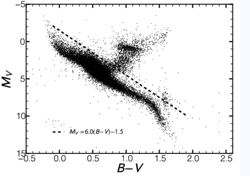
Figure 1.— All Hipparcos  stars in our $\leq$120 pc parent sample fall below the prescribed absolute magnitude cut to remove giant stars. The parent sample is restricted to stars with d $\leq$ 120 pc to reduce the effects of reddening from interstellar cirrus. Stars are also restricted to positions outside the galactic plane ($|b|\geq 5^{\circ}$) to minimize photometric contamination from confusion or interstellar cirrus.

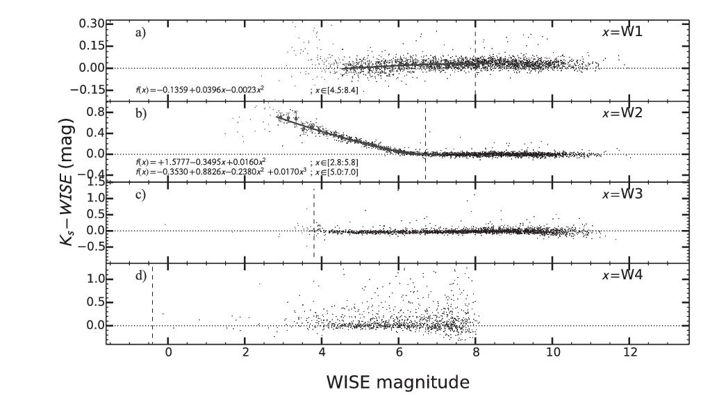
Figure 2.— 2MASS $K_{s}$-WISE vs. WISE relations used for correcting systematics in saturated $W1$ (a) and $W2$ (b) photometry. The empirical $K_{s}$-WISE vs. WISE distributions are a combination of bright B8–A9 dwarf stars from our science sample with fainter $B-V<0.10$ mag A0 stars from the Tycho-2 Spectral Type Catalog (Wright et al., 2003). Saturation limits for each WISE band are shown with vertical dashed lines. Polynomials were fit to the saturated portions of the $K_{s}-W1$ vs. $W1$ and $K_{s}-W2$ vs. and $W2$ distributions to model the systematic trends and correct the saturation. Two polynomials were fit to the saturated $W2$ data to account for the knee between 5.4 mag and 6.7 mag. A discontinuity of $\lesssim$0.010 mag was allowed at $W2=5.4$ mag. The $W3$ (c) and the $W4$ (d) photometry appears self-consistent throughout and does not require correction.

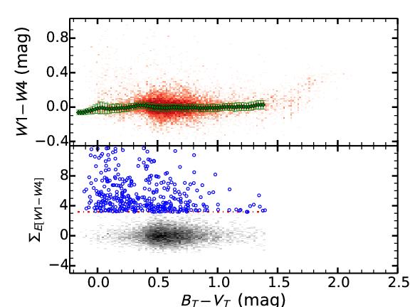
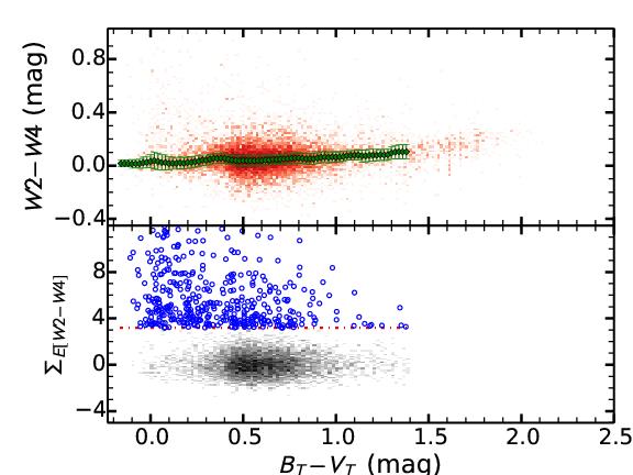
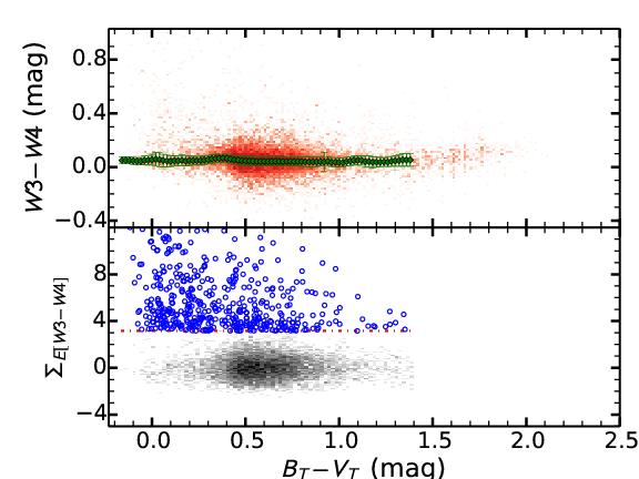
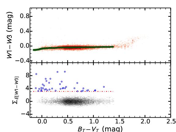
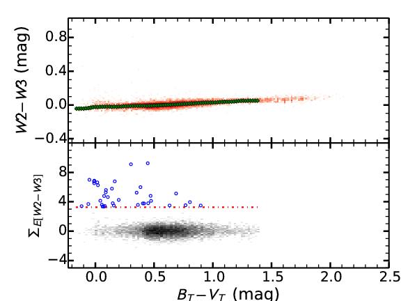
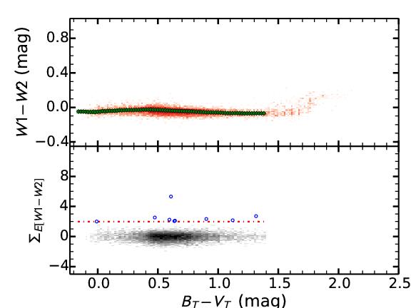
Figure 3.— Top Half of Each Panel: WISE vs. Tycho-2 $B_{T}-V_{T}$ color-color diagrams of our parent sample stars (red). The green diamonds in each panel follow the running mean of the parent sample. We eliminated stars outside the $-0.17<B_{T}-V_{T}<1.4$ mag range from all of our analysis. Bottom Half of Each Panel: Plots of the significance $\Sigma_{E}$  of the color excess as a function of $B_{T}-V_{T}$. These are residuals of the subtraction of the photospheric running mean, normalized to the 1 $\sigma$ scatter. The stars selected as debris disk candidates in the parent sample are denoted by open blue circles. These are more significant than the confidence limit $CL$ thresholds shown by the dashed purple lines. $CL=$99.5% for $W4$ excesses, 98% for $W3$ excesses, and 95% for $W2$ excesses.

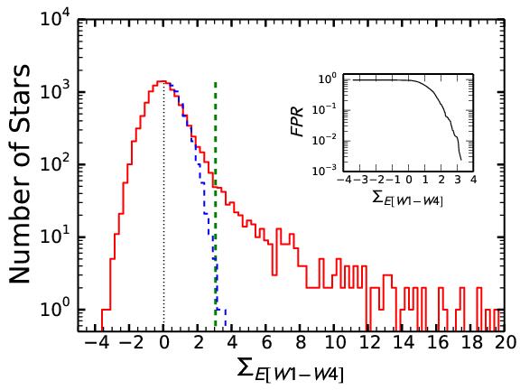
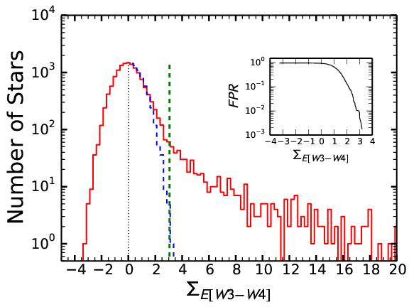
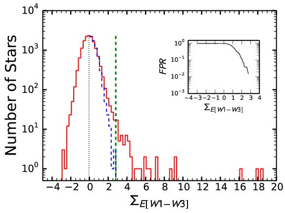
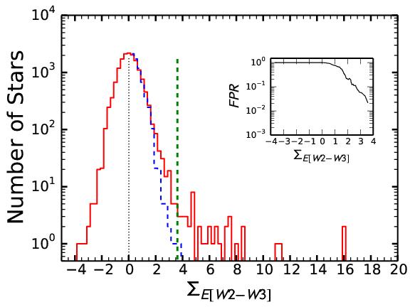
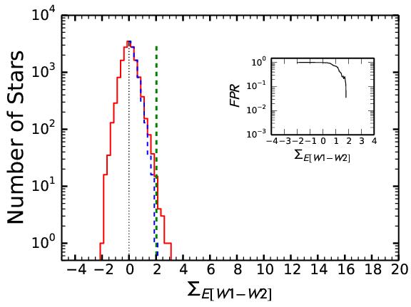
Figure 4.— Distributions of the significance of the color excess $\Sigma_{E}$ for the stars in our parent sample for each WISE  color. We assume that the negative excesses, where $\Sigma_{E}$  $<$ 0, are representative of the intrinsic random and systematic noise in the data. A reflection of the negative excess histogram around 0 (dashed histogram) is thus representative of the false positive excess expectation. We define the FPR at a given $\Sigma_{E}$ as the ratio of the cumulative numbers of $>$$\Sigma_{E}$ excesses in the positive tails of the dashed and solid histograms. The vertical dashed lines indicate the FPR thresholds for each $Wi-Wj$ color, above which we identify all stars as probable debris disk hosts. The insets show the FPR for each distribution.

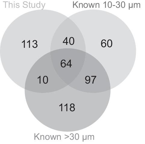
Figure 5.— A comparison between excess detections in this study and previously reported excesses at mid-IR (10–30${\rm\mu m}$ ) and far-IR ($\lambda\geq 30$ ${\rm\mu m}$ ) wavelengths. Only stars that are within 75 pc of the Sun with galactic latitudes $5^{\circ}$ above or below the galactic plane are included in this comparison. Our study is focused on Hipparcos stars, while the previous studies include non-Hipparcos stars, too. Data for these stars was obtained from the following sources: Sylvester & Mannings (2000), Habing et al. (2001), Metchev et al. (2004), Beichman et al. (2005), Chen et al. (2005), Chen et al. (2005), Low et al. (2005), Beichman et al. (2006a), Beichman et al. (2006b), Chen et al. (2006), Moór et al. (2006), Smith et al. (2006), Su et al. (2006), Rhee et al. (2007), Rhee et al. (2007), Trilling et al. (2007), Wyatt et al. (2007), Hillenbrand et al. (2008), Meyer et al. (2008), Rebull et al. (2008), Rhee et al. (2008), Roberge & Weinberger (2008), Trilling et al. (2008), Bryden et al. (2009), Carpenter et al. (2009), Dahm & Carpenter (2009), Kóspál et al. (2009), Lawler et al. (2009), Moór et al. (2009), Morales et al. (2009), Plavchan et al. (2009), Su et al. (2009), Koerner et al. (2010), Moerchen et al. (2010), Smith & Wyatt (2010), Dodson-Robinson et al. (2011), Eiroa et al. (2011), Moór et al. (2011), Morales et al. (2011), Zuckerman et al. (2011), Kennedy et al. (2012), Urban et al. (2012) and Wu et al. (2013).

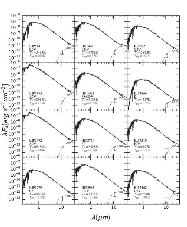
Figure 6.— SEDs of probable debris disk-host stars in our science sample. The dashed lines and solid data points correspond to the fitted model NextGen photosphere and to $BVJHK_{s}$ photometry from the Hipparcos  Catalogue and 2MASS  Point Source Catalog. Fluxes plotted as closed circles were used in the fit, and fluxes plotted as stars—excesses above the photosphere—were not used in the fit. Cool blackbody curves (dash-dotted line) were fitted to the excess fluxes (open diamonds) at the $W3$ and/or $W4$ wavelengths. The combined photosphere and excess emission for each star is plotted as a solid black line.

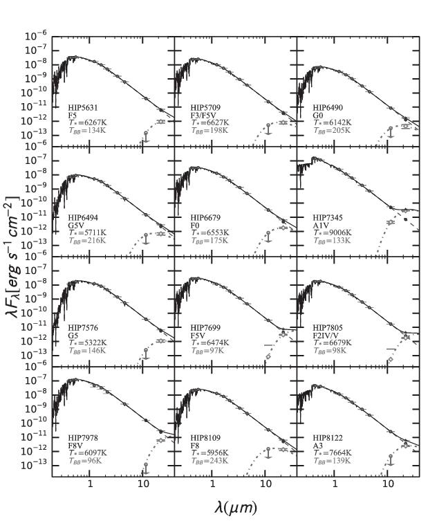
Figure 6.— continued.

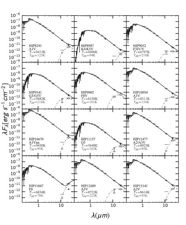
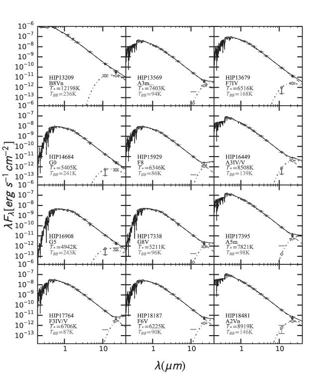
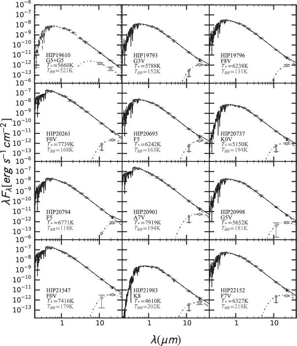
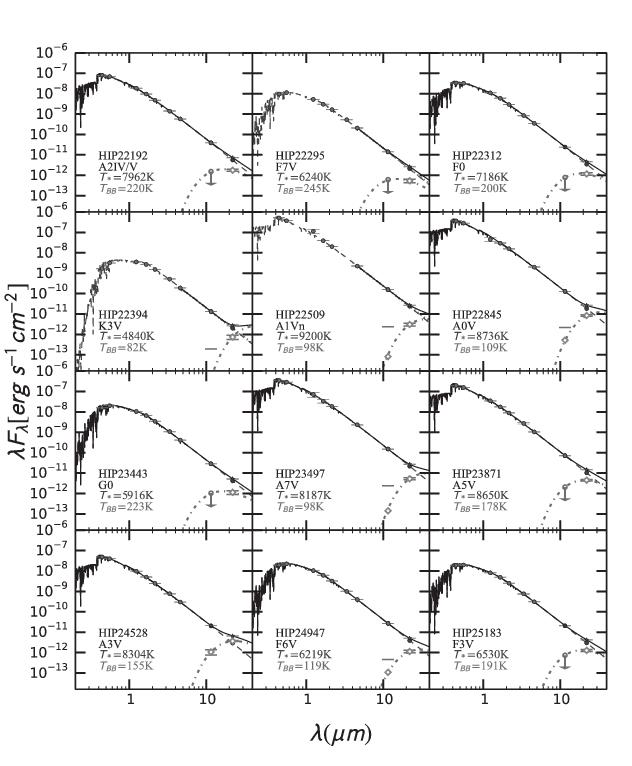
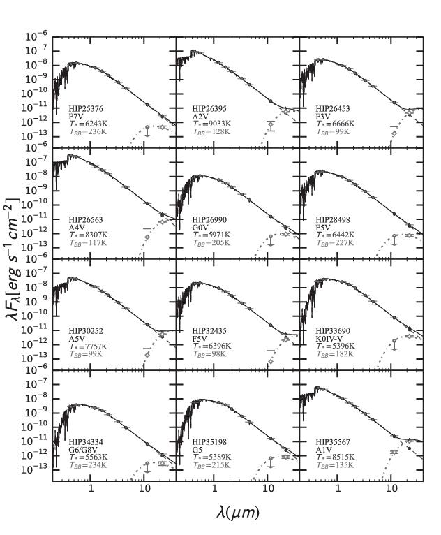
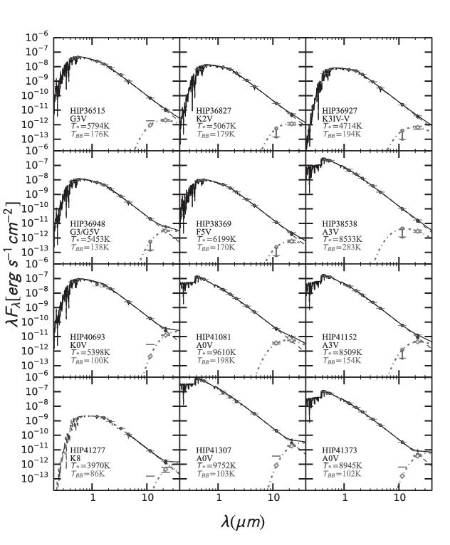
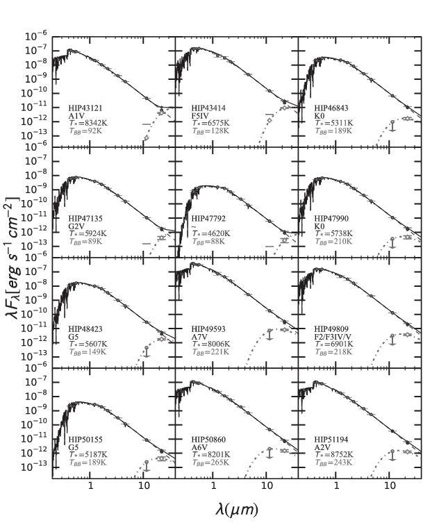
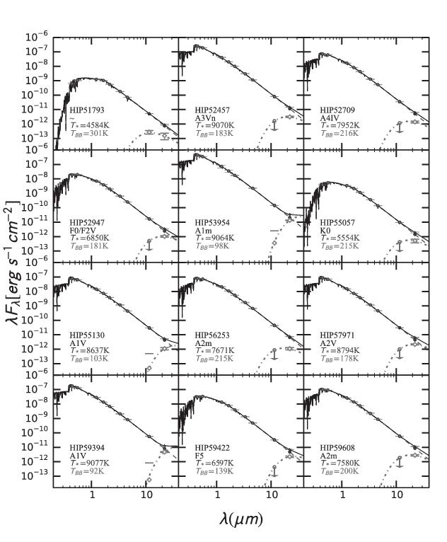
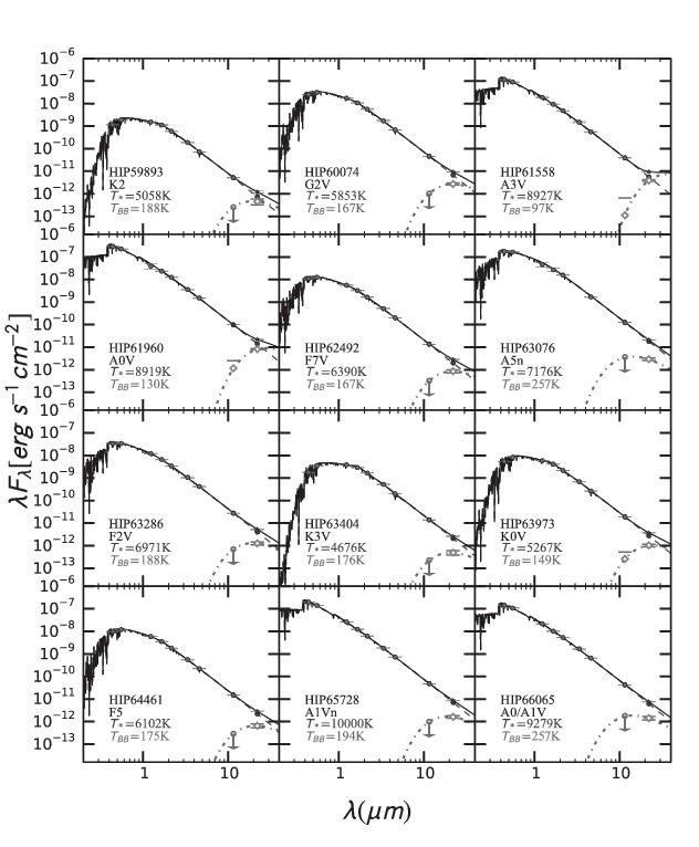
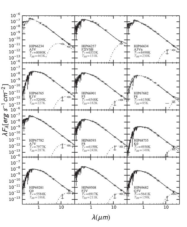
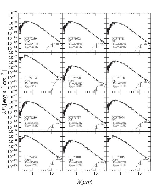
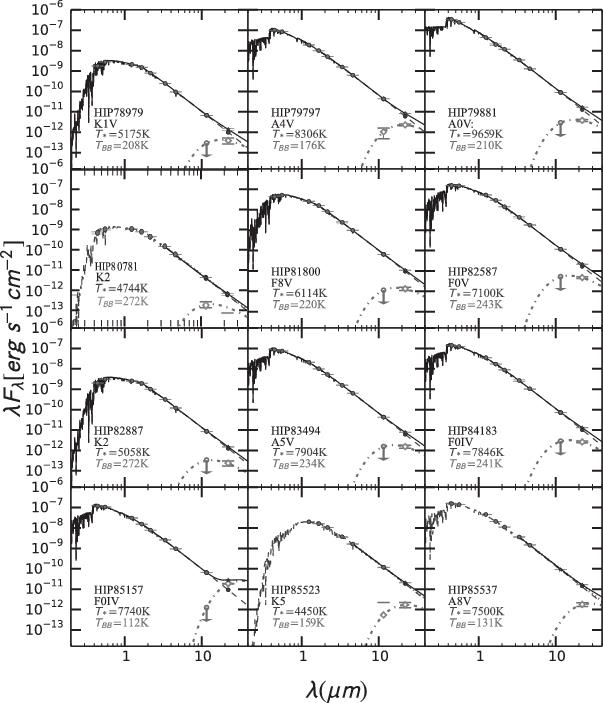
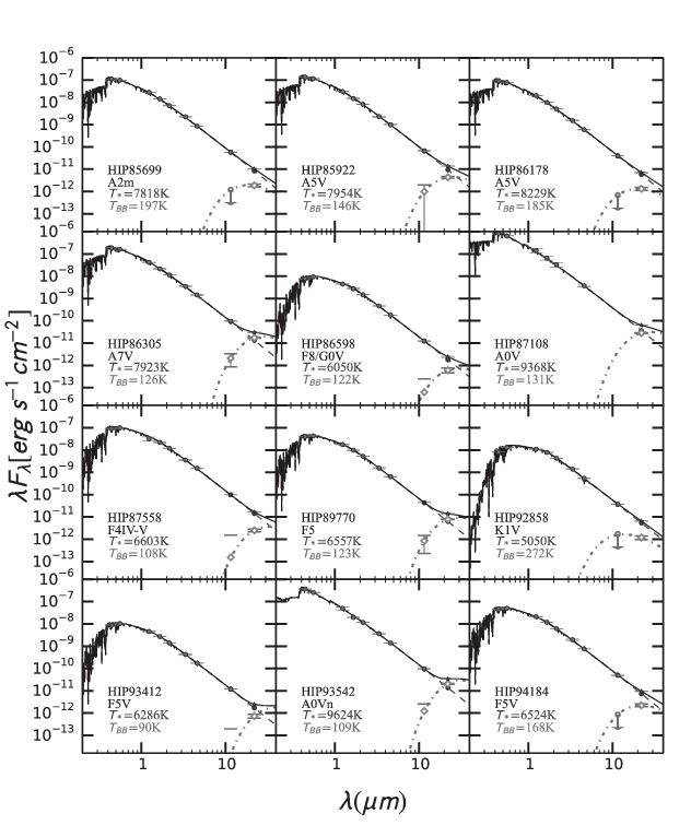
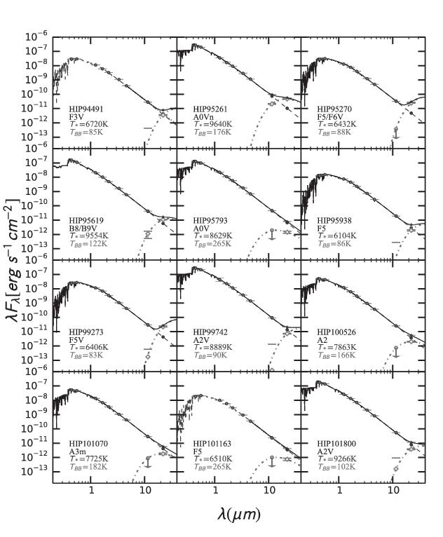
Figure 6.— continued.

Figure 6.— continued.

Figure 6.— continued.

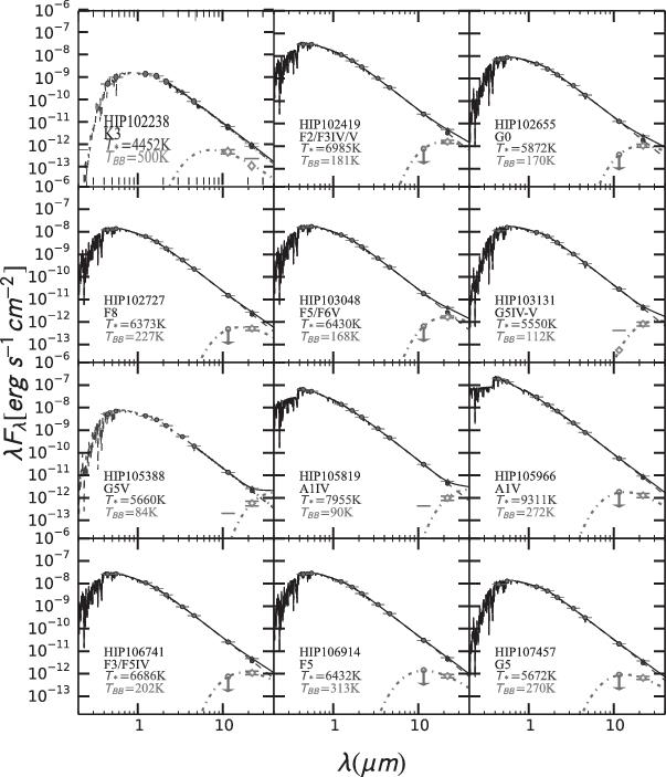
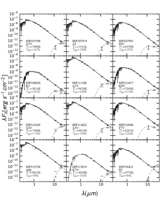
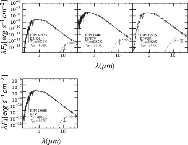
Figure 6.— continued.

Figure 6.— continued.

Figure 6.— continued.

Figure 6.— continued.

Figure 6.— continued.

Figure 6.— continued.

Figure 6.— continued.

Figure 6.— continued.

Figure 6.— continued.

Figure 6.— continued.

Figure 6.— continued.

Figure 6.— continued.

Figure 6.— continued.

Figure 6.— continued.

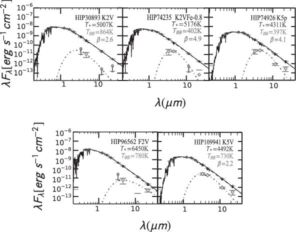
Figure 7.— SEDs of stars with $W2$ excesses above the 95% confidence level. The stellar photosphere (dashed line) was fit to the $BVJHK_{s}$ photometry only. A blackbody was fit to the excess around the F star HIP 96562. In the cases of the four K stars, we fit modified blackbody functions (dot-dashed lines) to the WISE excess fluxes (diamonds), or to the WISE 3$\sigma$ upper limit fluxes (open circles with downward arrows) when the excesses were negative. The K-star SEDs require a wide range of grain-emissivity index values ($\beta$), some of which are unphysical. The nature of these excesses remains uncertain at this time.

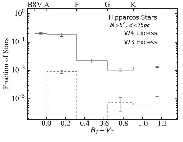
Figure 8.— Fraction of WISE excesses detected in this survey as a function of spectral type from our science sample. To determine the excess fraction at each wavelength, we chose the most sensitive color combination.

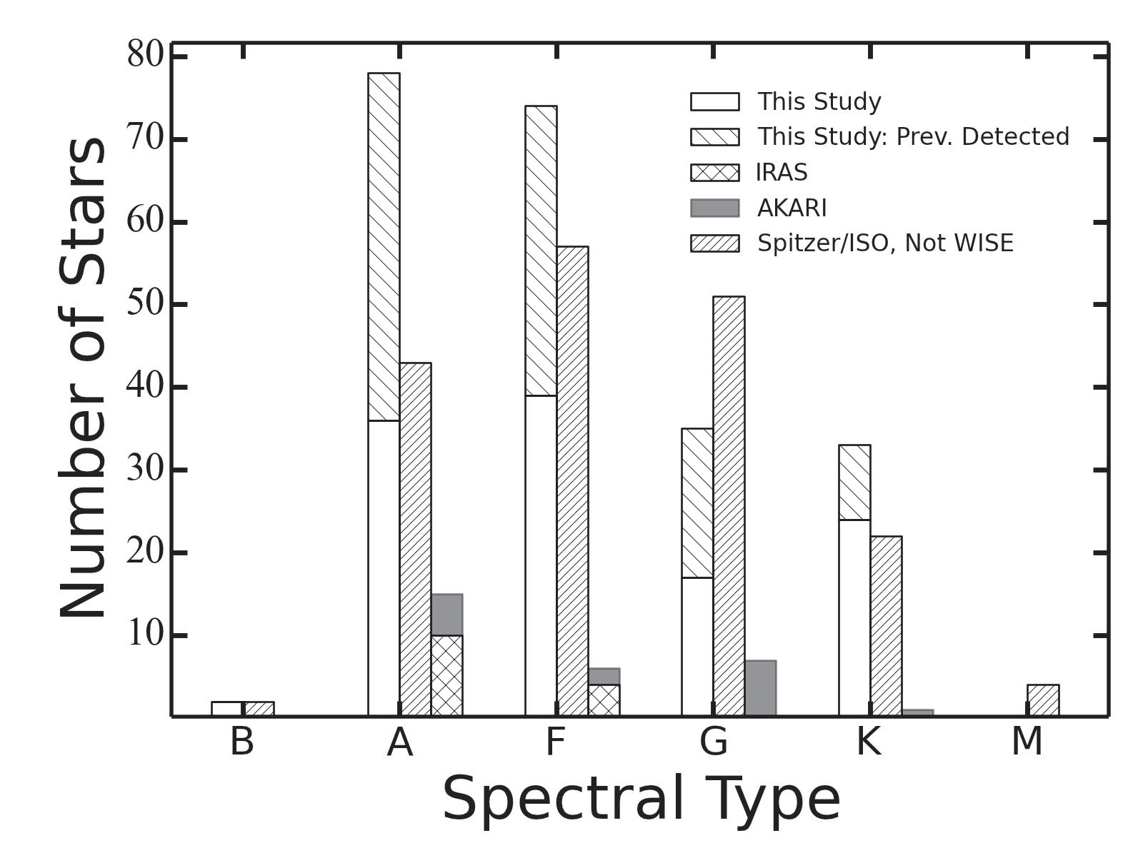
Figure 9.— Distribution of excesses detected as a function of spectral type using WISE  (this paper) compared to IR excess stars detected by pointed surveys and other all-sky surveys. All the excesses are compared at wavelengths between 10–30$\micron$, for stars that are outside the galactic plane $|b|\geq 5^{\circ}$ and within 75 pc of the Sun.

References

- Avenhaus et al. (2012) Avenhaus, H., Schmid, H. M., & Meyer, M. R. 2012, A&A, 548, A105
- Backman & Paresce (1993) Backman, D. E., & Paresce, F. 1993, in Protostars and Planets III, ed. E. H. Levy & J. I. Lunine, 1253
- Beichman et al. (2005) Beichman, C. A., et al. 2005, ApJ, 622, 1160
- Beichman et al. (2006a) Beichman, C. A., et al. 2006a, ApJ, 652, 1674
- Beichman et al. (2006b) Beichman, C. A., et al. 2006b, ApJ, 639, 1166
- Biller et al. (2007) Biller, B. A., et al. 2007, ApJS, 173, 143
- Bryden et al. (2009) Bryden, G., et al. 2009, ApJ, 705, 1226
- Bryden et al. (2006) Bryden, G., et al. 2006, ApJ, 636, 1098
- Carpenter et al. (2009) Carpenter, J. M., et al. 2009, ApJS, 181, 197
- Chen et al. (2005) Chen, Jura, M., Gordon, K. D., & Blaylock, M. 2005, The Astrophysical Journal, 623, 493
- Chen et al. (2005) Chen, C. H., et al. 2005, ApJ, 634, 1372
- Chen et al. (2006) Chen, C. H., et al. 2006, The Astrophysical Journal Supplement Series, 166, 351
- Cohen et al. (2003) Cohen, M., Wheaton, W. A., & Megeath, S. T. 2003, AJ, 126, 1090