Holographic Holes in Higher Dimensions

Abstract

We extend the holographic construction of hole from AdS₃ to higher dimensions. In particular, we show that the Bekenstein-Hawking entropy of codimension-two surfaces in the bulk with planar symmetry can be evaluated in terms of the ‘differential entropy’ in the boundary theory. The differential entropy is a certain quantity constructed from the entanglement entropies associated with a family of regions covering a Cauchy surface in the boundary geometry. We demonstrate that a similar construction based on causal holographic information fails in higher dimensions, as it typically yields divergent results. We also show that our construction extends to holographic backgrounds other than AdS spacetime and can accommodate Lovelock theories of higher curvature gravity.

1 Introduction

Remarkably, the entropy of a black hole is embodied in the spacetime geometry, as expressed by the Bekenstein-Hawking (BH) formula beks ; BH:1973 :

$$S_{\textrm{\tiny BH}}=\frac{{\cal A}}{4G_{\textrm{\tiny N}}}\,,$$ (1)

where $\cal A$ is the area of (a cross-section of) the event horizon. In fact, this expression applies equally well to any Killing horizon Jacobson:2003wv , including de Sitter DS and Rindler ray horizons, as well as horizons in higher dimensions. Further, this expression (1) extends to a more general geometric formula, the ‘Wald entropy’, to describe the horizon entropy in gravitational theories with higher curvature interactions WaldEnt .

Recently, it was proposed that the above expression (1) has much wider applicability and serves as a characteristic signature for the emergence of a semiclassical spacetime geometry in a theory of quantum gravity new1 . More precisely, the spacetime entanglement conjecture of new1 may be stated as follows: In a theory of quantum gravity, for any sufficiently large region in a smooth background spacetime, one may consider the entanglement entropy between the degrees of freedom describing the given region with those describing its complement. First, ref. new1 conjectures that in this context, the contribution describing the short-range entanglement will be finite and have a local geometric description in terms of the geometry at the entangling surface. Further, the leading contribution from this short-range entanglement will be given precisely by the BH formula (1). Of course, an implicit assumption is that the usual Einstein-Hilbert action (as well as, possibly, a cosmological constant term) emerges as the leading contribution to the low energy effective gravitational action. As demonstrated in misha9 , higher curvature corrections to the gravitational action will also control the subleading contributions to this entanglement entropy, which take a form similar to those in the Wald entropy.

One simple observation giving support for this spacetime entanglement conjecture comes from gauge/gravity duality. In their seminal work rt1 , Ryu and Takayanagi conjectured a simple and elegant prescription for a holographic calculation of entanglement entropy in the boundary theory — see also rt2 ; rt3 . In particular, the entanglement entropy for a specified spatial region $A$ in the boundary and its complement is evaluated with

$$S(A)=\mathrel{\mathop{\rm ext}_{\scriptscriptstyle{a\sim A}}{}\!\!}\left[\frac{{\cal A}(a)}{4G_{\textrm{\tiny N}}}\right]$$ (2)

where $a\sim A$ indicates that the bulk surface $a$ is homologous to the boundary region $A$ head ; fur06a . The symbol ‘ext’ indicates that one should extremize the area over all such surfaces $a$. This prescription applies where the bulk is described by classical Einstein gravity and was recently proved for static backgrounds in aitor . Hence in this context, we are evaluating the Bekenstein-Hawking formula (1) on surfaces which generally do not correspond to a horizon in the bulk. Further the usual bulk/boundary dictionary equates an entropy on the boundary theory to an entropy in the bulk theory and hence from these holographic calculations, we can infer that the Bekenstein-Hawking formula in eq. (2) literally yields an entropy for the corresponding bulk surface $a$.

One may note, however, that the prescription for holographic entanglement entropy picks out a special class of bulk surfaces, i.e., extremal surfaces with a specified set of asymptotic conditions at the boundary of the bulk geometry. In contrast, the spacetime entanglement conjecture maintains that the BH formula would determine the entropy associated with any such surface, whether or not it is extremal, as well as for closed surfaces that do not reach the asymptotic boundary. However, there is no contradiction here. The entanglement entropy in the boundary theory has a unique value once the entangling surface and the state are specified and hence the holographic prescription would be incomplete without specifying a specific bulk surface on which to evaluate eq. (1). We may also add that there have also been some earlier discussions that more general bulk surfaces may also give some entropic measure of correlations in the boundary theory mark1 ; causal0 .

Recently, ref. hole studied whether a precise meaning could be given to the spacetime entanglement conjecture in a more general context in the AdS/CFT correspondence. In particular, this paper investigated whether the entropy $S_{\textrm{\tiny BH}}={\cal A}/4G_{\textrm{\tiny N}}$ for closed curves in the bulk of AdS₃ could appear as an observable in the two-dimensional boundary CFT. Strong sub-additivity was used to argue that this quantity should be bounded by the following combination of entanglement entropies

$$E=\sum_{k=1}^{n}\left[\,S(I_{k})-S(I_{k}\cap I_{k+1})\,\right]\,,$$ (3)

where the intervals $I_{k}$ cover a time slice in the boundary. In fact, it was shown that applying the holographic prescription (2) in a particular continuum limit leads to the saturation of this bound with $E=S_{\textrm{\tiny BH}}$ — we review the details of their construction in section 2. They suggested that $E$ corresponds to the ‘residual’ entropy which measures the uncertainty in the density matrix of the global state if one tries to reconstruct the density matrix from observations of an infinite family of observers making observations in the causal development of each interval. As the expression in eq. (3) will be central to our discussions, we will establish the nomenclature here that $E$ is the ‘differential entropy.’

The remainder of the paper is organized as follows: In section 2, we review the calculation of the Bekenstein-Hawking entropy of closed curves in the bulk of three-dimensional AdS space in terms of the differential entropy of a set of intervals in the boundary CFT. However, we provide a perspective that is distinct from the original presentation in hole . In particular, we introduce the geometric concept of the ‘outer envelope,’ which allows for more intuitive picture of this construction. In section 2.2, we also point out some geometric subtleties, which call for generalizations of both the differential entropy and the outer envelope. In section 3, we extend these calculations to higher dimensions. In particular, we study the situation where a time slice in the boundary is covered by a family of overlapping strips to evaluate the BH entropy (1) of a bulk surface. This construction limits our analysis to cases with planar symmetry, i.e., the profile of the bulk surface can only depend on one of the boundary coordinates. In section 4, we consider using causal holographic information as the basis for this construction in higher dimensions but show that quite generally this approach does not yield finite results. In section 5, we extend the discussion to more general holographic backgrounds and in section 5.1, we show that these results can be extended to also include bulk gravity theories where the gravitational entropy has a more general form. In particular, the latter include higher curvature theories known as Lovelock gravity, as shown in appendix A. We close with a brief discussion of our results and future directions in section 6.

2 Holographic holes in AdS₃ and the outer envelope

In this section, we discuss some of the key results of hole . In particular, the BH entropy (1) for closed curves in three-dimensional AdS space, i.e., $S_{\textrm{\tiny BH}}=($length of curve$)/(4G_{\textrm{\tiny N}})$, can be evaluated in terms of the combination of entanglement entropies given in eq. (3) for the two-dimensional boundary CFT. However, we will provide a more intuitive geometric description of their construction, which in particular, makes no reference to accelerated observers in the bulk or time intervals in the boundary theory. As we describe below, a key ingredient of our approach will be the ‘outer envelope,’ which in the simplest cases can be seen as the boundary of the union of bulk regions associated with each of the boundary intervals matt . However, as we will see in section 2.2, this simple definition must be generalized in certain situations. Another difference from hole is that the present calculations will be formulated in terms of Poincaré coordinates, rather than global coordinates.

A central point in the discussion below and in hole is a property of entanglement entropy known as ‘strong subadditivity’ ssa , which is an inequality that holds quite generally in comparing entanglement entropies of various components of a quantum system. In particular, for two overlapping regions, $I_{1}$ and $I_{2}$, in a QFT, this inequality can be expressed as

$$S(I_{1}\cup I_{2})+S(I_{1}\cap I_{2})\leq S(I_{1})+S(I_{2})\,.$$ (4)

Let us recall the holographic proof of this strong subadditivity or rather the proof that the RT prescription (2) for holographic entanglement entropy satisfies this inequality (4).

For simplicity, we assume that the bulk geometry is static (and so may then be easily analytically continued to a Euclidean spacetime). Now following head2 , we consider two overlapping regions, $I_{1}$ and $I_{2}$, on a constant (Euclidean) time slice in the boundary theory. Figure 1a illustrates the regions on the boundary of the AdS spacetime, as well as the corresponding extremal surfaces in the bulk which are used to evaluate the holographic entanglement entropy. In particular, for $S(I_{1})$ and $S(I_{2})$, we have the blue arcs, $i_{1}$ and $i_{2}$, respectively. Similarly, $S(I_{1}\cup I_{2})$ and $S(I_{1}\cap I_{2})$ are evaluated with the RT prescription (2) using the green arcs, $i_{1\cup 2}$ and $i_{1\cap 2}$, respectively. Now the assumption of a static bulk has two simplifying effects. First, as is implicit in the figure, all of the relevant extremal surfaces lie in the same constant time slice in the bulk geometry and second, the extremization procedure in eq. (2) picks out the bulk surfaces with the minimal surface area, rather than just saddle-points. As a result of the first property, the two surfaces, $i_{1}$ and $i_{2}$, intersect in the bulk along some codimension-three surface, denoted by the point $p_{\textrm{int}}$ in figure 1a. Now in this holographic construction, we can consider exchanging the interconnections of the original surfaces at this intersection and then re-express the right-hand side of eq. (4) in terms of the areas of the resulting surfaces, which we denote as $k_{1\cup 2}$ and $k_{1\cap 2}$. We illustrate this re-arrangement with the red ($k_{1\cup 2}$) and yellow ($k_{1\cap 2}$) arcs in figure 1b. As indicated by the subscripts, $k_{1\cup 2}$ and $k_{1\cap 2}$ are homologous to $i_{1\cup 2}$ and $i_{1\cap 2}$, respectively. However, since the latter are the extremal surfaces within their respective homology classes, we have ${\cal A}(i_{1\cup 2})<{\cal A}(k_{1\cup 2})$ and ${\cal A}(i_{1\cap 2})<{\cal A}(k_{1\cap 2})$, and therefore the desired inequality (4) is satisfied. Here we might add that a proof of strong subadditivity (4) for holographic entanglement entropy in nonstatic backgrounds was recently formulated but is much more elaborate aron2 .

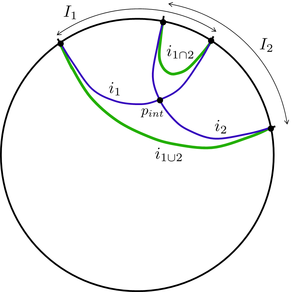
(a)

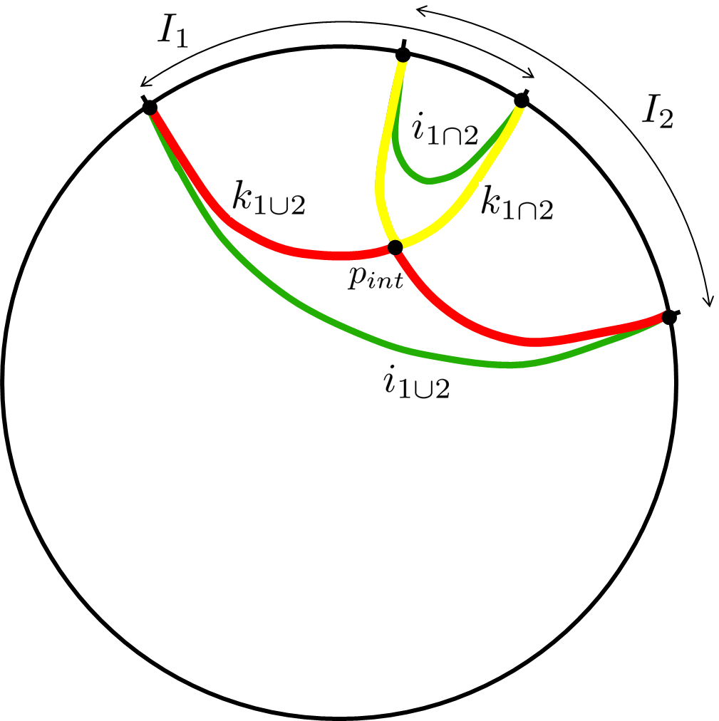
(b)

Figure 1: (Color online) Proof of strong subadditivity in a holographic framework: (a) Two intervals on the boundary of AdS₃ in global coordinates. The blue arcs indicate the geodesics used to evaluate $S(I_{1})$ and $S(I_{2})$, while the green arcs are those which determine $S(I_{1}\cup I_{2})$ and $S(I_{1}\cap I_{2})$. (b) Rearranging the interconnection of the blue arcs at their intersection produces two new curves in the same homology classes as the green arcs. However, the lengths of the red and yellow curves must be longer than that of the homologous green arcs.

For the remainder of the discussion in this section, we will focus on a three-dimensional bulk spacetime, however, the observations made here are readily extended to the configurations in higher dimensions that are examined in the subsequent sections. Returning to figure 1b, we will denote the surface $k_{1\cup 2}$ as the ‘outer envelope.’ More generally of a family of intervals $I_{k}$, we can define the outer envelope as the boundary of the union of all of the bulk regions enclosed by the geodesics determining $S(I_{k})$ according to the RT prescription matt . Further for our example here, let us denote the Bekenstein-Hawking entropy (1) evaluated on this surface as

$${\hat{S}}(I_{1},I_{2})=\mathcal{A}(k_{1\cup 2})/4G_{\textrm{\tiny N}}\,,$$ (5)

which we will loosely refer to as the ‘entropy of the outer envelope.’ Of course, the endpoints of $k_{1\cup 2}$ are defined by the endpoints of the union of the corresponding boundary intervals. However, as illustrated in figure 2a, the full geometry of the outer envelope is not just a function of $I_{1}\cup I_{2}$, but rather it depends on the details of the partition of this boundary region. Hence, the entropy ${\hat{S}}$ is indicated to be a function of $I_{1}$ and $I_{2}$ individually in eq. (5).

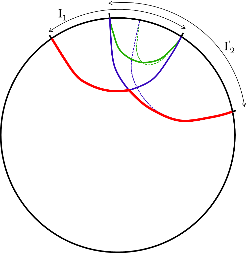
(a)

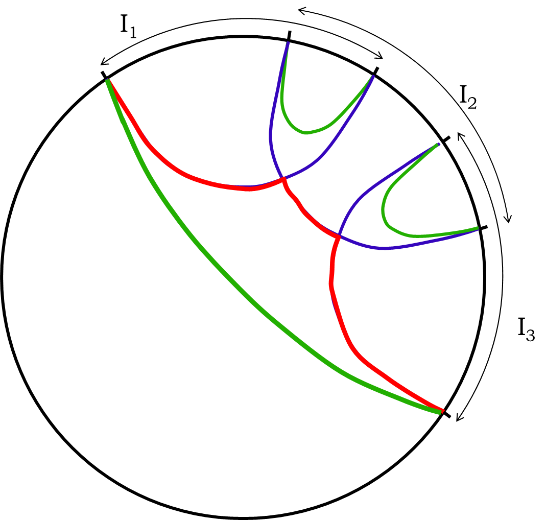
(b)

Figure 2: (Color online) (a) This figure illustrates that the outer envelope depends on the details of the individual boundary intervals, not just their union. (b) An example with three boundary intervals and the corresponding outer envelope (in red).

Now following the reasoning presented in proving strong subadditivity for holographic entanglement entropy above, one can easily verify that the following inequalities hold

$$S(I_{1}\cup I_{2})\leq{\hat{S}}(I_{1},I_{2})\leq S(I_{1})+S(I_{2})-S(I_{1}\cap I_{2})\,.$$ (6)

For example, $S(I_{1}\cup I_{2})\leq{\hat{S}}(I_{1},I_{2})$ holds because $i_{1\cup 2}$ and $k_{1\cup 2}$ are in the same homology class but $i_{1\cup 2}$ is the extremal surface chosen to minimize the BH entropy within this class. Now if one has $n$ consecutive overlapping intervals on the boundary, these arguments can be extended to establish the following generalization of eq. (6)

$$S(\cup I_{k})\leq{\hat{S}}(\{I_{k}\})\leq\sum_{k=1}^{n}S(I_{k})-\sum_{k=1}^{n-1}S(I_{k}\cap I_{k+1})\,.$$ (7)

An example of the corresponding surfaces are illustrated in figure 2b for three boundary intervals.

We will primarily be interested in the case where, in fact, the intervals are chosen to cover the entire boundary, as illustrated in figure 3. In this case, we write the corresponding inequalities as

$$S(\cup I_{k})\leq{\hat{S}}(\{I_{k}\})\leq\sum_{k=1}^{n}S(I_{k})-\sum_{k=1}^{n}S(I_{k}\cap I_{k+1})\,.$$ (8)

Note that eqs. (7) and (8) are distinct because the second sum in that latter includes an $n$’th term hole , which should be interpreted as $S(I_{n}\cap I_{n+1})=S(I_{n}\cap I_{1})$. In this scenario where the entire boundary is covered, the outer envelope forms a closed curve in the bulk. Note that in the case when the bulk geometry is empty AdS space, as illustrated in figure 3a, the entanglement entropy for the union of all the intervals vanishes. This result arises from the bulk perspective since the prescription for holographic entanglement entropy (2) instructs us to find an extremal surface which is homologous to the entire boundary. Hence we are considering closed surfaces in the bulk but upon extremizing within this class, the minimal area is found when the surface simply shrinks to a point and the area vanishes. In contrast, no extremization appears in the construction of the outer envelope and so the corresponding entropy ${\hat{S}}(\{I_{k}\})$ remains finite. From the boundary perspective, the previous vanishing is natural because empty AdS₃ is dual to the vacuum of the boundary CFT and so the corresponding entropy vanishes. In fact, when the bulk is dual to any pure state in the boundary theory, the entanglement entropy for the union of all the intervals must similarly vanish, i.e., $S(\cup I_{k})=S(|\psi\rangle\langle\psi|)=0$. Of course, as illustrated in figure 3b, if the bulk is a (stationary) black hole geometry, then $S(\cup I_{k})$ is non-vanishing. Here, the desired extremal surface corresponds to (the bifurcation surface of) the horizon and the corresponding entanglement entropy is just the thermodynamic entropy of the dual thermal ensemble in the boundary theory. In this instance, the outer envelope still defines a larger entropy, i.e., ${\hat{S}}(\{I_{k}\})\geq S(\cup I_{k})=S(\rho_{\textrm{therm}})$.

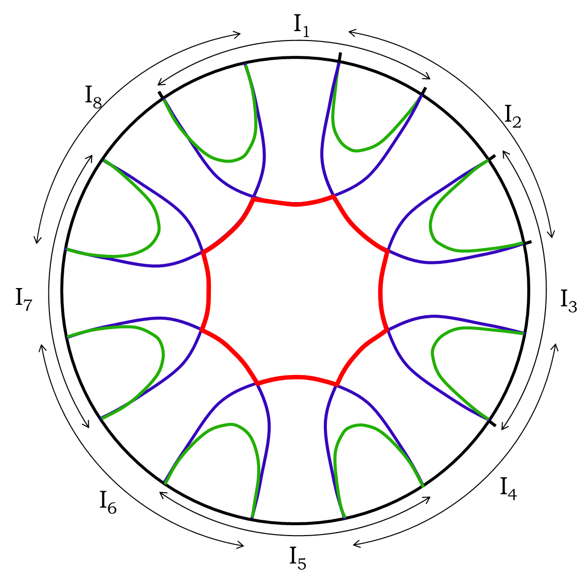
(a)

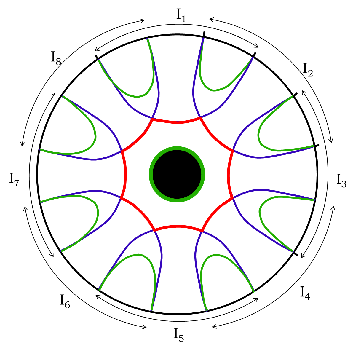
(b)

Figure 3: (Color online) Eight intervals and their outer envelope, which forms a closed curve in the bulk, (a) in empty AdS space and (b) in an AdS black hole spacetime. In case (a), the entanglement entropy of the global boundary state vanishes while it is non-vanishing in case (b).

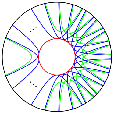
(a)

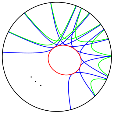
(b)

Figure 4: (Color online) (a) In the continuum limit of many identical intervals, the outer envelope becomes a circle of a fixed radius. (b) The continuum limit of many intervals whose length varies continuously produces a smooth outer envelope with a profile that varies in the bulk.

Above, we have introduced a class of closed curves in the bulk which are constructed as the outer envelope of a series of extremal surfaces determining the holographic entanglement entropies of some ordered set of intervals which partitions an entire time slice of the boundary. In general, eq. (8) indicates that the BH entropy of these closed curves is bounded below by the entanglement entropy of the boundary state and bounded above by a certain combination of entanglement entropies of the boundary intervals and their intersections. Now following hole , we extend these observations with the following construction (which be described in detail below): First, we keep the length of the individual intervals fixed but take the number of intervals equally spaced around the boundary to infinity. In this limit, the outer envelope becomes a smooth circle in the bulk with a fixed radius $R$, as shown in figure 4a, and the corresponding Bekenstein-Hawking entropy is simply ${\hat{S}}(\{I_{k}\})=2\pi R/4G_{\textrm{\tiny N}}$. The remarkable discovery in hole is that the second inequality in eq. (8) is in fact saturated in this limit, namely

$$\frac{2\pi R}{4G_{\textrm{\tiny N}}}=\sum_{k=1}^{\infty}\left[\,S(I_{k})-S(I_{k}\cap I_{k+1})\,\right]\,,$$ (9)

Further, with an appropriate extension of this continuum limit illustrated in figure 4, one finds the same equality holds for a general closed curve in the bulk,

$$\frac{\mathcal{A}(\textrm{bulk curve})}{4G_{\textrm{\tiny N}}}=\sum_{k=1}^{\infty}\left[\,S(I_{k})-S(I_{k}\cap I_{k+1})\,\right]\,.$$ (10)

Hence the two-dimensional boundary theory appears to have ‘observables’ corresponding to the BH entropy of arbitrary closed curves in the bulk of AdS₃. Before proceeding to higher dimensions, let us describe the construction for AdS₃ in more detail, for the case where it is adapted to Poincaré coordinates.

2.1 Holographic holes in AdS₃

To begin, recall the AdS₃ written in Poincaré coordinates

$$ds^{2}=\frac{L^{2}}{z^{2}}(dz^{2}-dt^{2}+dx^{2})\,.$$ (11)

Now if we wish to evaluate the holographic entanglement entropy of an interval of width $\Delta x$, the extremal surface simply takes the form of a semi-circle in these coordinates rt1 ; rt2 , i.e.,

$$z^{2}+x^{2}=(\Delta x/2)^{2}\,,$$ (12)

and evaluating the length of this extremal curve yields

$$S(\Delta x)=\frac{L}{2G_{\textrm{\tiny N}}}\ \log\!\left(\frac{\Delta x}{\delta}\right)\,,$$ (13)

where $\delta$ is the short-distance cut-off in the boundary theory, which is introduced with a cut-off surface in the bulk at $z=z_{\textrm{min}}=\delta$. Of course, upon substituting $c=3L/2G_{\textrm{\tiny N}}$, this holographic result (13) reproduces the universal result which applies for any two-dimensional CFT frank1 ; cardy1 .

For simplicity, let us begin by considering the Bekenstein-Hawking entropy for a surface in the bulk at a fixed $z=z_{*}$, as illustrated in figure 5. To regulate the area of this surface, we will impose that the $x$ direction is periodic with period $\ell_{1}$. One should think of the latter as some infrared regulator scale and so we assume that $\ell_{1}\gg\Delta x$. Now given the bulk metric (11), we find the BH entropy of the surface is given by

$$\frac{\mathcal{A}(z=z_{*})}{4\,G_{\textrm{\tiny N}}}=\frac{L\ \ell_{1}}{4G_{\textrm{\tiny N}}\,z_{*}}\,.$$ (14)

Now to begin, we consider a series of $n$ equally spaced intervals $I_{k}$ with a fixed width $\Delta x$, which cover the boundary. We choose $\Delta x=2z_{*}$ so that the corresponding extremal semi-circles (12) in the bulk are all tangent to the desired surface at $z=z_{*}$. Now, the intuition is that the latter surface emerges as the outer envelope of these semi-circles in the ‘continuum’ limit where $n\to\infty$. Hence, we first confirm that the entropy formula (14) is reproduced by ${\hat{S}}(\{I_{k}\})$ in the continuum limit. As illustrated in figure 5, it is useful to chose an angular coordinate along the semi-circles with:

$$z=z_{*}\,\cos\theta\,,\qquad x=x_{c,k}+z_{*}\,\sin\theta\,,$$ (15)

where $x_{c,k}$ is the midpoint of the corresponding interval $I_{k}$ on the boundary. With $n$ intervals on the boundary, the spacing between, e.g., their midpoints is simply given by $\ell_{1}/n$ and hence to determine the contribution of an individual semi-circle to the full length of the outer envelope, we must integrate $\theta$ over the range $[-\theta_{0},\theta_{0}]$ where

$$\sin\theta_{0}=\frac{\ell_{1}}{2n\,z_{*}}\,.$$ (16)

Then the Bekenstein-Hawking entropy associated with the full outer envelope becomes

$${\hat{S}}(\{I_{k}\}) = \frac{n}{4G_{\textrm{\tiny N}}}\,2\,\int_{0}^{\theta_{0}}d\theta\frac{L}{\cos\theta}$$ (17)

$$= \frac{nL}{4G_{\textrm{\tiny N}}}\ \log\!\left(\frac{1+\frac{\ell_{1}}{2n\,z_{*}}}{1-\frac{\ell_{1}}{2n\,z_{*}}}\right)\,.$$

Finally, it is straightforward to see that in the limit $n\to\infty$, this result (17) simplifies to precisely the desired entropy given in eq. (14).

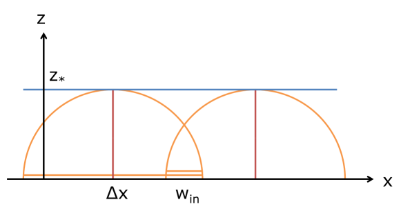
Figure 5: (Color online) A bulk surface with a constant profile $z=z_{*}$. The two intersecting semi-circles of radius $r=z_{*}$ in AdS₃ are the extremal bulk surfaces determining the holographic entanglement entropy for two overlapping boundary intervals of length $\Delta x=2z_{*}$.

Now we turn to the differential entropy (3) of the same family of intervals $I_{k}$. Recall the width of each interval was $\Delta x=2z_{*}$. Hence with $n$ equally spaced intervals on the boundary of length $\ell_{1}$, we find that the length of the intersections $I_{k}\cap I_{k+1}$ is given by

$$w_{\textrm{in}}=2z_{*}-\frac{\ell_{1}}{n}\,,$$ (18)

as is seen in figure 5. Hence combining the above results, the differential entropy (3) becomes

$$E(\{I_{k}\})=\sum_{k=1}^{n}\left[\,S(I_{k})-S(I_{k}\cap I_{k+1})\,\right] = \frac{nL}{2G_{\textrm{\tiny N}}}\ \left[\log\!\left(\frac{2z_{*}}{\delta}\right)-\log\!\left(\frac{w_{\textrm{in}}}{\delta}\right)\right]$$ (19)

$$= -\frac{nL}{2G_{\textrm{\tiny N}}}\ \log\!\left(1-\frac{\ell_{1}}{2nz_{*}}\right)\,.$$

Again, we can easily show that in the limit $n\to\infty$, this result (19) simplifies to the desired entropy in eq. (14).

As an aside, let us combine eqs. (17) and (19) to establish

$$E(\{I_{k}\})-{\hat{S}}(\{I_{k}\})=-\frac{nL}{4G_{\textrm{\tiny N}}}\ \log\!\left[1-\left(\frac{\ell_{1}}{2nz_{*}}\right)^{2}\right]\geq 0\,.$$ (20)

Hence eq. (20) explicitly shows that at finite $n$, $E(\{I_{k}\})>{\hat{S}}(\{I_{k}\})$, as expected, and it is only in the continuum limit with $n\to\infty$, that we have $E(\{I_{k}\})={\hat{S}}(\{I_{k}\})$.

Next let us consider a bulk surface of varying profile $z(x)$, as illustrated in figure 6. In this case, evaluating the Bekenstein-Hawking formula (1) on this curve yields

$$\frac{\mathcal{A}(z=z(x))}{4\,G_{\textrm{\tiny N}}}=\frac{L}{4G_{\textrm{\tiny N}}}\ \int_{0}^{\ell_{1}}\!dx\,\frac{\sqrt{1+z^{\prime 2}}}{z}\,,$$ (21)

where again we have assumed that the $x$ direction is periodic with period $\ell_{1}$.

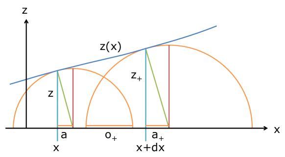
Figure 6: (Color online) A bulk surface with a varying profile $z=z(x)$. The radius of the semi-circles tangent to this surface varies with $x$ and hence the length of the corresponding boundary intervals is also a function of $x$. Further, the center of the boundary interval is displaced from the tangent point along the $x$-axis by some distance $a(x)$.

In this case, we will work directly in the continuum limit with an infinite number of boundary intervals. The key idea is to find a family of intervals $I_{k}$ such that there is a dual semi-circle in the bulk which is tangent to each point along the chosen surface. The geometry for two neighboring intervals is shown in figure 6. Here we choose points on the bulk surface which are separated infinitesimally along the $x$ direction, i.e., the points at $x$ and $x\pm dx$ which sit at $z=z(x)$ and $z_{\pm}=z(x\pm dx)$ in the bulk. Note that generally the midpoint of the corresponding intervals is displaced from the position of the tanget point because of the nonvanishing slope of $z(x)$. We denote this shift as $a(x)$, as shown in figure 6, and examining the geometry, we find

$$z^{\prime}(x)=\frac{a(x)}{z(x)}\,.$$ (22)

Now let us denote the width of the corresponding intervals as $\Delta x(x)$ and since $\Delta x(x)=2\,r(x)$ where $r(x)$ is the radius of the corresponding semi-circle in the bulk, we find

$$\Delta x(x)=2\,z(x)\,\sqrt{1+z^{\prime}(x)^{2}}\,,$$ (23)

using eq. (22). Finally, if we use $o_{\pm}$ to denote the overlaps between the interval corresponding to the point at $x$ and those at $x\pm dx$, then we can show

$$o_{\pm}=\frac{1}{2}\left(\Delta x(x)+\Delta x(x\pm dx)\right)\pm\left(a(x)-a(x\pm dx)\right)-dx\,.$$ (24)

Writing eq. (22) as $a=z\,z^{\prime}$, we can expand the combination of shifts appearing above to first order in $dx$ to find

$$\pm\left(a(x)-a(x\pm dx)\right)=-a^{\prime}dx=-(z^{\prime 2}+z\,z^{\prime\prime})dx\,.$$ (25)

Combining this expression with eq. (23), the overlaps in eq. (24) can be written as

$$o_{\pm}=2z\sqrt{1+z^{\prime 2}}-dx\left(1+z^{\prime 2}+zz^{\prime\prime}\right)\pm\frac{1}{2}\Delta x^{\prime}dx\,.$$ (26)

Note that as may have been expected to leading order in the continuum limit, the overlap between neighboring intervals is complete, i.e., $o_{\pm}=\Delta x(x)+O(dx)$.

In the above analysis (and in figure 6), we implicitly assumed that the slope of the profile was positive (i.e., $z^{\prime}\geq 0$) at the points $x$ and $x\pm dx$. However, our results are readily adapted to also cover the case of negative slopes. In particular, when $z^{\prime}$ is negative, we see that $a$ changes its sign from eq. (22). But the $\pm$ in front of $(a-a_{\pm})$ in eq. (24) also needs to be flipped. Hence the final formula (26) covers the case of negative slopes as well. Henceforth for simplicity, we will assume that $z^{\prime}$ is positive without loss of generality.

Now following hole , the final steps in the analysis is simplified if we replace the differential entropy (3) with the following ‘averaged’ expression

$$E=\sum_{k=1}^{n}\left[\,S(I_{k})-\frac{1}{2}S(I_{k}\cap I_{k+1})-\frac{1}{2}S(I_{k-1}\cap I_{k})\,\right]\,.$$ (27)

Then combining eq. (26) with the expression for the holographic entanglement entropy (13), we find

$$S(I_{k})-\frac{1}{2}S(I_{k}\cap I_{k+1}) - \frac{1}{2}S(I_{k-1}\cap I_{k})=\frac{L}{4G_{\textrm{\tiny N}}}\ \log\left(\frac{\Delta x^{2}}{o_{+}\,o_{-}}\right)$$ (28)

$$\simeq \frac{L}{4G_{\textrm{\tiny N}}}\frac{1+z^{\prime 2}+zz^{\prime\prime}}{z\,\sqrt{1+z^{\prime 2}}}\,dx+O(dx^{2})\,.$$

Hence the differential entropy (27) becomes

$$E(\{I_{k}\}) = \frac{L}{4G_{\textrm{\tiny N}}}\int_{0}^{\ell_{1}}\frac{1+z^{\prime 2}+zz^{\prime\prime}}{z\,\sqrt{1+z^{\prime 2}}}\,dx$$ (29)

$$= \frac{L}{4G_{\textrm{\tiny N}}}\int_{0}^{\ell_{1}}\left[\frac{\sqrt{1+z^{\prime 2}}}{z}+\frac{z^{\prime\prime}}{\sqrt{1+z^{\prime 2}}}\right]dx$$

$$= \frac{L}{4G_{\textrm{\tiny N}}}\left[\int_{0}^{\ell_{1}}\!dx\,\frac{\sqrt{1+z^{\prime 2}}}{z}+{\rm arcsinh}(z^{\prime})\biggl{|}_{0}^{\ell_{1}}\right]\,.$$

Of course, the final contribution cancels due to the periodic boundary conditions which were chosen at the outset of our calculation. However, one can see that this term will vanish with other choices of boundary conditions, as well. For instance, if the $x$ direction was of infinite extent, it would suffice to impose $z^{\prime}\to 0$ as $x\to\pm\infty$. In any event, the remaining integral precisely matches the expression in eq. (21) for the BH entropy (1) of the bulk surface with profile $z(x)$.

2.2 Some geometric subtleties

Our previous discussion makes the implicit assumption that the profile $z(x)$ of the bulk curve varies relatively slowly. In particular, we assume that at each point along the curve, the curvature of the profile is small enough that the curve remains outside of the corresponding semi-circle that is tangent at this point. Therefore we will examine next the changes in the previous construction when this assumption no longer holds. One observation is that we will have to revise the definition of the ‘outer envelope’ introduced at the beginning of this section to extend our discussion to cover these situations. However, we will first examine a simple example to gain some qualitative understanding of the (unexpected) behavior that arises in this situation.

In figure 7, we illustrated a simple bulk curve where some of the semi-circles tangent to this surface extend further into the bulk beyond the curve. The (red) profile shown there is flat with $z=z_{*}$ apart from a bump, where it rises to $z=z_{\textrm{max}}$ and then returns to $z=z_{*}$ over a fairly narrow interval. The figure also shows the semi-circles that are tangent to points on the profile that are regularly spaced along the $x$-axis. The (green) semi-circles tangent to the points near the peak of the bump clearly extend into the bulk beyond the (red) curve and so these are the points of primary interest here. The endpoints for the corresponding intervals on the AdS boundary at $z=0$ (which corresponds to the thick black line in the figure) are defined by the intersection of the semi-circles with $z=0$. The center of each semi-circle, which is also the center of the corresponding boundary interval, is also indicated in figure 7 for each of the points along the bulk curve. In regions where the bulk profile is flat, the $x$ positions of the tangent point in the bulk and the center of the corresponding interval on the boundary actually coincide. However, when the profile starts to curve up into the bulk, we can see that the center points on the boundary begin to ‘accelerate’ ahead of the tangent points. This acceleration stops where the slope $dz/dx$ reaches its maximum, i.e., at the point denoted 5. This point is also the first one for which the tangent semi-circle is not contained entirely within the bulk profile. As indicated in the figure, at this stage, the center points actually begin to move backwards along the $x$-axis — even though, the corresponding tangent points in the bulk are still moving forward. This reverse motion of the center points continues for the tangent points across the peak of the bump, which corresponds to all of those points for which the tangent semi-circle extends beyond the bulk profile. This process ends where the slope $dz/dx$ is most negative, i.e., at the point marked 9. At this tangent point, the corresponding center point on the boundary is behind along the $x$-axis. For the subsequent points, the tangent semi-circles are all contained within the bulk curve and the center points are again moving forward towards larger values of $x$.

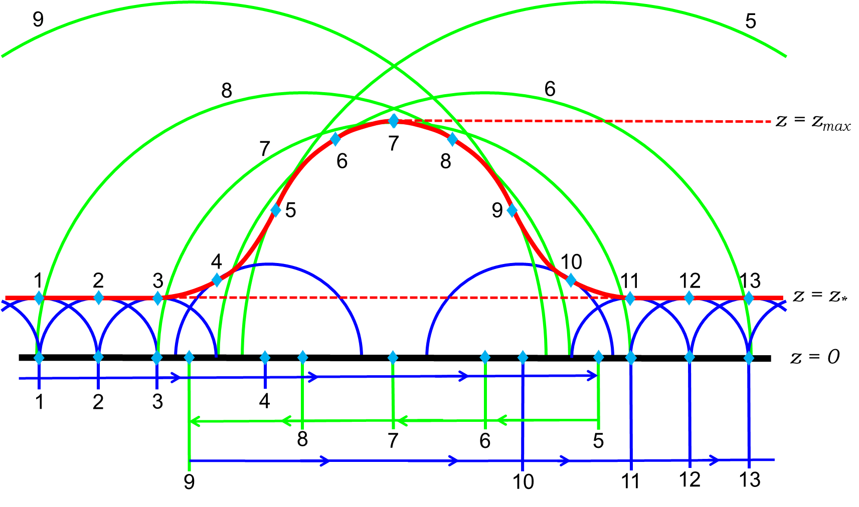
Figure 7: (Color online) A bulk surface (red) which is flat with $z=z_{*}$ apart from a bump rising to $z=z_{\textrm{max}}$ and then returning to $z=z_{*}$ over a fairly narrow interval. The semi-circles tangent to points regularly spaced in $x$ along this curve are shown in blue and green. The green semi-circles extend into the bulk beyond the surface. The centers of the corresponding boundary intervals are also shown.

The example in figure 7 seems to connect the tangent semi-circle extending beyond the bulk surface and the backward motion of the center point of the boundary interval. So we would like use our results in the previous subsection to verify that this behavior above is, in fact, a general property of this construction. First, if we consider the point on the bulk curve to be at $x$, then the center of the corresponding boundary interval is given by

$$x_{c}(x)=x+a(x)=x+z\,z^{\prime}\,,$$ (30)

using eq. (22). Given this expression, we see that $x_{c}=x$ if and only if $z^{\prime}=0$ while $z^{\prime}>0$ yields $x_{c}>x$ and $z^{\prime}<0$ yields $x_{c}<x$. We can also evaluate the derivative

$$x_{c}^{\prime}=1+z^{\prime 2}+z\,z^{\prime\prime}\,,$$ (31)

and next we would like to show that $x_{c}^{\prime}<0$ implies that the corresponding semi-circle in the bulk extends beyond the curve $z(x)$. A Taylor expansion of the bulk profile around some value of $x$ yields

$$z(x+\delta x)=z(x)+z^{\prime}(x)\,\delta x+\frac{1}{2}z^{\prime\prime}(x)\,\delta x^{2}+\cdots\,.$$ (32)

Now the semi-circle, which is tangent to the curve at $x$, is described by the following profile

$$z_{sc}(\tilde{x};x)=\sqrt{r(x)^{2}-(\tilde{x}-x_{c}(x))^{2}}\,,$$ (33)

where the radius is given by $r(x)^{2}=z(x)^{2}+a(x)^{2}$. Hence using our previous results, we find an expansion about $x$ yields, i.e., with $\tilde{x}=x+\delta x$,

$$z_{sc}(x+\delta x;x)=z(x)+z^{\prime}(x)\,\delta x-\frac{1}{2}\left(\frac{1+z^{\prime 2}}{z}\right)\,\delta x^{2}+\cdots\,.$$ (34)

Comparing eqs. (32) and (34), we see that the first two terms in these expansions match, which of course was ensured by the construction. Hence, the question of whether or not the semi-circle remains below the bulk surface is determined, at least locally, by the quadratic term in the expansions. In particular, the semi-circle extends beyond the curve if

$$z^{\prime\prime}<-\frac{1+z^{\prime 2}}{z}\,.$$ (35)

Now comparing eqs. (31) and (35), we see that the above inequality corresponds precisely to the condition for $x_{c}^{\prime}<0$, as expected.

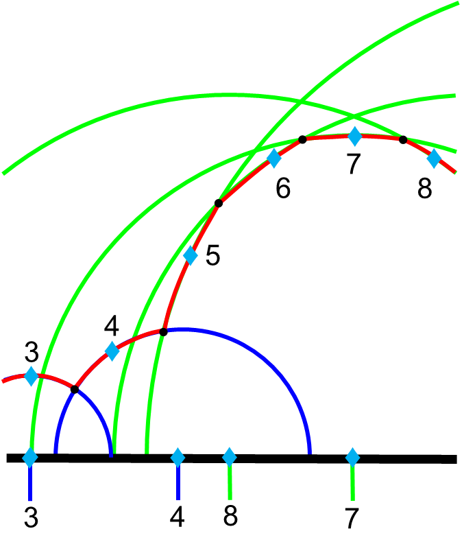
Figure 8: (Color online) A portion of figure 7, which illustrates that segments of the tangent semi-circles can still be used to give a good approximation to the desired bulk curve. Hence a suitable definition for the ‘outer envelope’ is simply the union of these segments.

We originally defined the ‘outer envelope,’ as the curve in the bulk is comprised of the outermost segments of the extremal surfaces defining the entanglement entropies appearing in the differential entropy (3). While this definition works in the simplest cases, it does not apply in the present case where these extremal surfaces extend beyond the bulk curve. However, as shown in figure 8, the bulk curve is still well approximated piece-wise by various segments of these extremal curves. If we examine this figure, we see the appropriate segments are simply those which extend along the extremal curves from the tangent point for a given interval $I_{k}$ to the first intersection with the extremal curves for the adjacent intervals, i.e., $I_{k-1}$ and $I_{k+1}$. Of course, these are perhaps the collection of segments which intuitively would give a good approximation to the bulk curve. Note that we will still refer to this collection as the ‘outer envelope,’ even though this nomenclature does not always give an accurate description of the union of these segments.

This case where the semi-circles extend beyond the bulk curve also calls for us to revise our definition of the differential entropy. Recall that this situation also corresponds to the center of the corresponding intervals moving in the negative direction along the $x$-axis. Hence let us consider the simplest example of two overlapping intervals, $I_{k}$ and $I_{k+1}$, for which the corresponding extremal curves in the bulk intersect, as shown in figure 9. Let introduce the notation, $x_{L,k}$ and $x_{R,k}$, to denote the left and right end-points of the interval $I_{k}$. The ‘standard’ case with $x_{c}^{\prime}>0$ is shown on the left of the figure, while the case with $x_{c}^{\prime}<0$ is illustrated on the right. Note that in both cases, the outer envelope is comprised of the two segments of the bulk semi-circles which extend from $x_{L,k}$ to $x_{R,k+1}$. Motivated by discussion of strong subadditivity, in both cases, we would bound the corresponding BH entropy ${\hat{S}}$ by taking the sum of the entanglement entropies $S(I_{k})$ and $S(I_{k+1})$ and subtracting of the entanglement entropy for the interval extending from $x_{R,k}$ to $x_{L,k+1}$. Of course, in the standard case with $x_{c}^{\prime}>0$, the latter corresponds to $S(I_{k}\cap I_{k+1})$. However, when $x_{c}^{\prime}<0$, the term which we subtract off is actually $S(I_{k}\cup I_{k+1})$! If we extend these observations to a general family of intervals $\{I_{k}\}$, the bound on the BH entropy of the outer envelope becomes

$${\hat{S}}(\{I_{k}\})\leq\sum S(I_{k})-\sum_{x_{c,k}<x_{c,k+1}}S(I_{k}\cap I_{k+1})-\sum_{x_{c,k}>x_{c,k+1}}S(I_{k}\cup I_{k+1})\,,$$ (36)

where $x_{c,k}$ denotes the center of the interval $I_{k}$. The right-hand side of this expression replaces eq. (3) as our definition of the differential entropy

$$E\equiv\sum_{k=1}^{n}S(I_{k})-\sum_{x_{c,k}<x_{c,k+1}}S(I_{k}\cap I_{k+1})-\sum_{x_{c,k}>x_{c,k+1}}S(I_{k}\cup I_{k+1})\,.$$ (37)

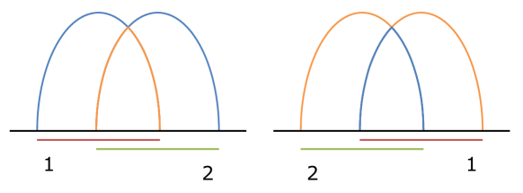
Figure 9: (Color online) Generalized outer envelope of two intervals indicated by the blue curve.

As a final geometric subtlety, let us consider whether or not we will ever encounter with our construction, the situation illustrated in figure 10 where one interval is completely enclosed by the next interval in the sequence, i.e., either $I_{k}\subset I_{k+1}$ or $I_{k}\supset I_{k+1}$. If such a situation occurred, it would of course produce a problem in defining the outer envelope, as the dual semi-circles in the bulk would not intersect anywhere. However, we can show that, in fact, this situation never arises in the continuum limit by showing that $x_{L}^{\prime}\,x_{R}^{\prime}\geq 0$ everywhere. Note that $x_{L}(x)=x_{c}(x)-r(x)$ and $x_{R}(x)=x_{c}(x)+r(x)$ and hence the desired inequality is

$$x_{c}^{\prime 2}-r^{\prime 2}\geq 0\,.$$ (38)

Recall that the derivative of the center point is given in eq. (31). Further with $r=\sqrt{z^{2}+a^{2}}$, one can easily show that

$$r^{\prime}=\frac{z^{\prime}\,x_{c}^{\prime}}{\sqrt{1+z^{\prime 2}}}$$ (39)

and hence, as desired,

$$x_{c}^{\prime 2}-r^{\prime 2}=\frac{x_{c}^{\prime 2}}{1+z^{\prime 2}}\geq 0\,.$$ (40)

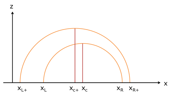
Figure 10: (Color online) No intersection between two neighboring tangent semicircles.

3 Planar holes in higher dimensions

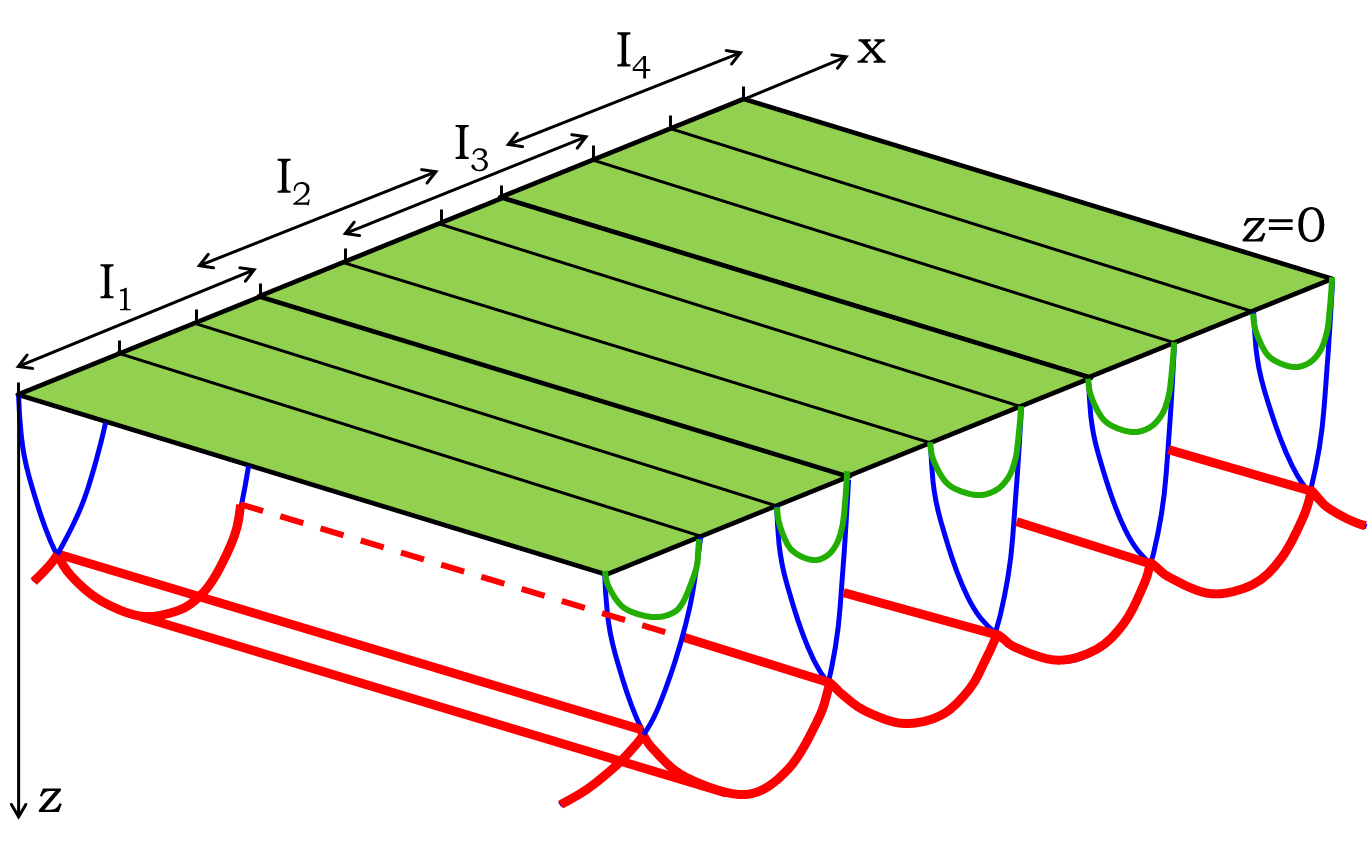
Figure 11: (Color online) Covering the boundary of AdS_d+1 with a family of overlapping strips.

We would like to explore whether the construction discussed in the previous section for a three-dimensional AdS bulk extends to the case of higher dimensions. As before, we will consider the case where the $d$-dimensional boundary geometry is simply flat space. Hence, we are working in Poincaré coordinates with

$$ds^{2}=\frac{L^{2}}{z^{2}}\left(dz^{2}-dt^{2}+d\vec{x}^{2}\right)\,,$$ (41)

where as usual, the AdS boundary is at $z=0$. As a simple first step, we will limit ourselves to considering the case where a constant time slice is partitioned by a family of overlapping strips or slabs, $\{I_{k}\}$, as shown in Figure 11. In general, we will allow the width of the strips to vary as we move along the orthogonal $x$-axis. Hence our intuition at this stage is that our construction will allow us to evaluate the Bekenstein-Hawking entropy for bulk surfaces with a planar symmetry. That is, we can accommodate bulk surfaces with a profile of the form $z=z(x)$. In order to regulate the area of these surfaces, we will impose that the $x$ direction is periodic with period $\ell_{1}$, as in section 2.1. Further, for simplicity, we also assume that the remaining spatial directions $x^{i}$ are periodic on a scale $\ell_{i}$ (for $i=2,\cdots,d-1$, while $i=1$ denotes $x$), in order to regulate the distances along the strips.

As the geometry of the boundary regions and their intersections are both strips, let us begin by recalling the result for the holographic entanglement entropy of a strip of width $\Delta x$ on the boundary of AdS_d+1 rt1 — see also gb

$$S(\Delta x)=\frac{L^{d-1}}{4G_{\textrm{\tiny N}}}\,\frac{\ell_{2}\cdots\ell_{d-1}}{d-2}\left(\frac{2}{\delta^{d-2}}-\frac{c_{d}^{d-1}}{\Delta x^{d-2}}\right)\,.$$ (42)

Here, $\delta$ is the usual short-distance cut-off in the boundary CFT and $c_{d}$ is a numerical constant given by

$$c_{d}=2\sqrt{\pi}\,\frac{\Gamma\left(\frac{d}{2d-2}\right)}{\Gamma\left(\frac{1}{2d-2}\right)}=\frac{\Delta x}{z_{*}}\,.$$ (43)

As noted above $c_{d}$ is also the ratio between the width $\Delta x$ of the boundary interval and the corresponding maximal height $z_{*}$ of the extremal surface in the bulk, which is used to evaluate the holographic entanglement entropy. Recall the logarithmic result (13) for the entanglement entropy in $d=2$ and so implicitly, we are assuming that $d\geq 3$ above. In this case, the profile of the extremal surface along $x$ direction is no longer a semicircle but rather a curve in ($z$,$x$)-plane governed by the differential equation rt1

$$\frac{dz}{dx}=\pm\left[\left(\frac{z_{*}}{z}\right)^{2d-2}-1\,\right]^{1/2}\,.$$ (44)

To begin, we consider a bulk surface with a constant profile, $z=z_{*}$ (and $t=0$). With the relevant geometry described above, the Bekenstein-Hawking entropy for this surface is given by

$$\frac{\mathcal{A}(z=z_{*})}{4\,G_{\textrm{\tiny N}}}=\frac{L^{d-1}\,\ell_{1}\ell_{2}\cdots\ell_{d-1}}{4G_{\textrm{\tiny N}}\,z_{*}^{d-1}}\,.$$ (45)

Now as in the previous section, we expect that this result will be reproduced by evaluating the differential entropy for a series of $n$ equally spaced strips $I_{k}$ with a fixed width $\Delta x$ and taking the continuum limit $n\to\infty$. In order that the extremal surfaces determining the holographic entanglement entropy of the individual strips are tangent to the desired bulk surface, we must choose $\Delta x=c_{d}\,z_{*}$ according to eq. (43). With $n$ strips equally spaced along the $x$ direction, which has a length $\ell_{1}$, the width of the intersections $I_{k}\cap I_{k+1}$ is simply

$$w_{\textrm{in}}=\Delta x-\frac{\ell_{1}}{n}\,.$$ (46)

Then the desired differential entropy (37) becomes

$$E = \lim_{n\to\infty}n(S(\Delta x)-S(w_{\textrm{in}}))$$ (47)

$$= \frac{L^{d-1}}{4G_{\textrm{\tiny N}}}\,\frac{\ell_{2}\cdots\ell_{d-1}}{d-2}\,c^{d-1}_{d}\,\lim_{n\to\infty}n\left(-\frac{1}{\Delta x^{d-2}}+\frac{1}{(\Delta x-\ell_{1}/n)^{d-2}}\right)$$

$$= \frac{L^{d-1}}{4G_{\textrm{\tiny N}}}\,\frac{\ell_{2}\cdots\ell_{d-1}}{d-2}\,c^{d-1}_{d}\,\lim_{n\to\infty}\left(\frac{(d-2)\ell_{1}}{\Delta x^{d-1}}+O(1/n)\right)$$

$$= \frac{L^{d-1}\,\ell_{1}\ell_{2}\cdots\ell_{n}}{4G_{\textrm{\tiny N}}\ z_{*}^{d-1}}\,.$$

Hence we see that that the construction in section 2.1 naturally extends to higher dimensions, at least for the case of a bulk surface with a constant profile.

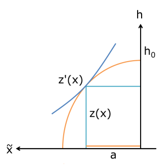
Figure 12: (Color online) A varying $z$ profile and its local tangent surface in AdS_d+1.

Given this success, we move to considering a bulk surface of nontrivial profile $z(x)$, i.e., still respecting the planar symmetry. Evaluating the BH formula (1) on such a surface in AdS_d+1 yields

$$\frac{\mathcal{A}(z=z(x))}{4\,G_{\textrm{\tiny N}}}=\frac{L^{d-1}}{4G_{\textrm{\tiny N}}}\,\ell_{2}\cdots\ell_{d-1}\,\int_{0}^{\ell_{1}}\!dx\,\frac{\sqrt{1+z^{\prime 2}}}{z^{d-1}}\,.$$ (48)

Now the first step towards evaluating the differential entropy (37) will be identifying the extremal surface which is tangent to the bulk surface at a given $x$, as shown in figure 12. We denote the profile of these extremal surfaces as $h(\tilde{x};x)$, where the second argument indicates that this extremal profile is tangent to the bulk surface at $\tilde{x}=x$, i.e.,

$$h(\tilde{x}=x;x)=z(x)\,,\qquad\frac{dh(\tilde{x};x)}{d\tilde{x}}\bigg{|}_{\tilde{x}=x}=z^{\prime}(x)\,.$$ (49)

Further, with eq. (44), we can write

$$\frac{dh}{d\tilde{x}}=\left[\left(\frac{h_{0}}{h}\right)^{2d-2}-1\,\right]^{1/2}\,,$$ (50)

where $h_{0}(x)$ is the maximal height to which the extremal profile $h(\tilde{x};x)$ rises in the bulk. Note that we have implicitly assumed that $dh/d\tilde{x}\geq 0$ above. In this case, as shown in figure 12, we consider the shift $a(x)$ along the $x$-axis between the tangent point $x$ and the midpoint of the boundary interval $x_{c}(x)$, where the extremal surface reaches $h_{0}$. This quantity is determined by

$$a(x)=\int_{x}^{x_{c}}d\tilde{x}=\int_{z(x)}^{h_{0}}\frac{h^{d-1}dh}{\sqrt{h_{0}^{2d-2}-h^{2d-2}}}=\frac{h_{0}}{2d-2}\,B\!\left[\left(\frac{z}{h_{0}}\right)^{2d-2}\right]\,,$$ (51)

where

$$B[x]=\int_{x}^{1}\frac{ds}{s^{\frac{d-2}{2d-2}}\sqrt{1-s}}\,.$$ (52)

On the other hand, combining eqs. (49) and (50) yields

$$z^{\prime 2}=\frac{h_{0}^{2d-2}}{z^{2d-2}}-1\,,$$ (53)

and therefore we may write

$$h_{0}=z(1+z^{\prime 2})^{1/(2d-2)}\,,\qquad a=\frac{h_{0}}{2d-2}\,B\!\left[\frac{1}{1+z^{\prime 2}}\right]\,.$$ (54)

Further, according to eq. (43), the width of the interval is

$$\Delta x=c_{d}\,h_{0}=c_{d}\,z\,(1+z^{\prime 2})^{1/(2d-2)}\,.$$ (55)

Having established these preparatory results, we now consider the intervals, $I_{k-1}$, $I_{k}$, $I_{k+1}$, for which the extremal bulk surfaces are tangent to the profile $z(x)$ at $x-dx$, $x$ and $x+dx$, respectively. Now as in eq. (24), we denote the width of the intersections $I_{k-1}\cap I_{k}$ and $I_{k}\cap I_{k+1}$, respectively, as

$$o_{\pm} = \frac{1}{2}(\Delta x(x)+\Delta x(x\pm dx))\pm(a(x)-a(x\pm dx))-dx$$ (56)

$$= \Delta x-\left(1+a^{\prime}\mp\Delta x^{\prime}\right)\,dx\,,$$

where, to leading order in $dx$, we have used

$$\Delta x(x\pm dx)=\Delta x(x)\pm\Delta x^{\prime}\,dx\,,\qquad a(x\pm dx)=a(x)\pm a^{\prime}\,dx\,.$$ (57)

From eq. (52), we have

$$\partial_{x}B\!\left[(z/h_{0})^{2d-2}\right]=-\frac{1}{s^{\frac{d-2}{2d-2}}\sqrt{1-s}}\frac{ds}{dx}\bigg{|}_{s=1/(1+z^{\prime 2})}=\frac{2z^{\prime\prime}}{(1+z^{\prime 2})^{1+1/(2d-2)}}\,,$$ (58)

and hence we may write

$$a^{\prime}=\frac{1}{2d-2}\left(B\,h_{0}^{\prime}+\frac{2zz^{\prime\prime}}{1+z^{\prime 2}}\right)\,.$$ (59)

Hence we can re-express the overlaps in eq. (56) as

$$o_{\pm}=\Delta x-\left[1+\frac{1}{2d-2}\left(B\,h_{0}^{\prime}+\frac{2zz^{\prime\prime}}{1+z^{\prime 2}}\right)\mp\Delta x^{\prime}\right]dx\,.$$ (60)

Now if we use an ‘averaged’ expression for the differential entropy, as in eq. (37), we find

$$E = \frac{L^{d-1}}{4G_{\textrm{\tiny N}}}\,\frac{\ell_{2}\cdots\ell_{d-1}}{d-2}\,c_{d}^{d-1}\int_{0}^{\ell_{1}}dx\,\left(-\frac{1}{\Delta x^{d-2}}+\frac{1}{2\,o_{+}^{d-2}}+\frac{1}{2\,o_{-}^{d-2}}\right)$$ (61)

$$= \frac{L^{d-1}}{4G_{\textrm{\tiny N}}}\,\frac{\ell_{2}\cdots\ell_{d-1}}{d-2}\,c_{d}^{d-1}\int_{0}^{\ell_{1}}dx\,\frac{1}{\Delta x^{d-1}}\left(\Delta x-\frac{o_{+}+o_{-}}{2}\right)\,,$$

$$= \frac{L^{d-1}}{4G_{\textrm{\tiny N}}}\,\frac{\ell_{2}\cdots\ell_{d-1}}{d-2}\,\int_{0}^{\ell_{1}}dx\,\frac{1}{h_{0}^{d-1}}\left[1+\frac{1}{2d-2}\left(B\,h_{0}^{\prime}+\frac{2zz^{\prime\prime}}{1+z^{\prime 2}}\right)\right]\,.$$

where we used eq. (54) to replace $h_{0}$ in the final line. Unfortunately, at this stage, the above expression looks quite different from the desired result (48). However, given our discussion in the previous section, we should expect that the integrands in these two expressions will differ by a total derivative. Hence we examine the difference between the two integrands and applying eqs. (54) and (58), one finds

$$\frac{1}{h_{0}^{d-1}}\left[1+\frac{1}{2d-2}\left(B\,h_{0}^{\prime}+\frac{2zz^{\prime\prime}}{1+z^{\prime 2}}\right)\right]-\frac{\sqrt{1+z^{\prime 2}}}{z^{d-1}}$$

$$\quad=\frac{d}{dx}\left(-\frac{1}{2(d-1)(d-2)}\frac{B}{h_{0}^{d-2}}+\frac{1}{d-2}\frac{z^{\prime}}{z^{d-2}\sqrt{1+z^{\prime 2}}}\right)\,.$$ (62)

The contribution of this total derivative vanishes as a boundary term and hence we have confirmed that the differential entropy again yields the BH entropy (1) for these bulk surfaces with a nontrivial profile $z(x)$.

3.1 Higher dimensions and higher curvatures

At this point, we would like to comment on extending these calculations to theories of higher curvature gravity in the bulk. In particular, we have shown that this discussion can accommodate Gauss-Bonnet gravity, in which a curvature-squared interaction proportional to the four-dimensional Euler density is included in the action. In a holographic context, this theory is often considered as a toy model to describe boundary CFT’s where the central charges are not all equal gb ; gb2 . As was first discussed in highc ; highc2 , holographic entanglement entropy can be calculated with a simple extension of the Ryu-Takayanagi prescription. In particular, one replaces the BH formula in eq. (2) with the following entropy functional

$$S_{\textrm{\tiny JM}}=\frac{1}{4G_{\textrm{\tiny N}}}\int_{\sigma}d^{d-1}x\sqrt{h}\left(1+\frac{2\lambda L^{2}}{(d-2)(d-3)}{\cal R}\right)$$ (63)

where $\cal R$ is the intrinsic curvature scalar for the bulk surface $\sigma$ and $\lambda$ is the (dimensionless) coupling for the curvature-squared terms in the action — see appendix A. This entropy functional was originally derived in studying black hole entropy for these theories tedJ . Nontrivial tests of holographic entanglement entropy were made with this prescription in highc ; highc2 , however, following aitor , this can now be derived xifriend .

At this point, we simply re-iterate that one is able to extend the previous discussion to incorporate these theories. In particular, the final result is that in the continuum limit, the differential entropy in the boundary theory, which is evaluated holographically using $S_{\textrm{\tiny JM}}$, matches the gravitational entropy in the bulk, which in this case is given by evaluating $S_{\textrm{\tiny JM}}$ on the bulk surface. The proof of this statement using the approach of the present section is rather lengthy and tedious. Hence we do not provide the details here and rather we note that this result is a corollary of the general proof appearing in section 5.

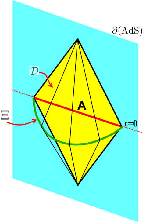
Figure 13: (Color online) The geometry relevant for the construction of causal holographic information — see the discussion in the main text.

4 Causal holographic information

Causal holographic information has been conjectured to be another interesting measure of entanglement in the boundary theory in a holographic framework causal0 ; aron . As we will comment below, it also has a natural connection to the discussion of holographic holes in hole . Hence let us review the definition of causal holographic information — see figure 13: One begins by specifying a region $A$ on a Cauchy surface in the boundary theory. One constructs the causal development $\cal D$ of this region, again in the boundary, and then extends null rays into the bulk from the boundary of $\cal D$ — past-directed light rays from the future boundary $\partial{\cal D}^{+}$ and future-directed light rays from the past boundary $\partial{\cal D}^{-}$. The envelope of these null rays enclose a bulk region, known as the causal wedge of $A$. The causal holographic information is then defined by evaluating the Bekenstein-Hawking entropy on the extremal surface on the boundary of the causal wedge, i.e.,

$$\chi(A)={\rm ext}\,\frac{{\cal A}(\Xi)}{4G_{\textrm{\tiny N}}}$$ (64)

where as in the holographic entanglement entropy, one extremizes over surfaces $\Xi$ which are homologous to $A$, but now confined to the boundary of the causal wedge.

Generally, the holographic entanglement entropy and the causal holographic information are distinct quantities. In particular, the extremal surface used to evaluate the holographic entanglement entropy of a given region typically probes deeper into the bulk than that appearing in the causal holographic information. An exception to this generic behavior arises with a spherical entangling surface and the boundary CFT in its vacuum state, i.e., the bulk is described by the pure AdS_d+1 vacuum. In this case, the corresponding causal wedge corresponds to an AdS-Rindler patch in the bulk and the extremal surface selected with the RT prescription (2) is precisely the bifurcation surface of the corresponding AdS-Rindler horizon chm ; eom1 . Hence the two extremal surfaces precisely match. Hence for a single interval in a two-dimensional boundary CFT, i.e., an AdS₃ bulk, the causal holographic information generally matches the holographic entanglement entropy. Hence the analysis of hole does not distinguish between these two quantities. In fact, this special feature is an essential part of the discussion in hole , since the contribution of each interval in eq. (3) is associated with the information which an accelerated bulk observer in the associated causal wedge can collect. Hence natural extension of the discussion in hole to higher dimensions might seem to involve constructing the surfaces in the bulk using the extremal surfaces used to evaluate the causal holographic information.

Hence we examine a version of our construction in the previous section using the causal holographic information. That is, we replace the entanglement entropies in the differential entropy (3) with the corresponding causal holographic information for the same intervals to define the ‘differential causal holographic information,’

$$E_{\chi}\equiv\sum_{k=1}^{n}\chi(I_{k})-\sum_{k=1}^{n}\chi(I_{k}\cap I_{k+1})\,.$$ (65)

Note that the causal holographic information does not satisfy the equivalent of strong subadditivity (4) and so this motivation is lacking when we apply eq. (65).

If we are considering a strip of width $\Delta x$ on the boundary of AdS_d+1, as in section 3, the corresponding extremal surface which defines the causal holographic information is a half cylinder defined by

$$z^{2}+(x-x_{c})^{2}=(\Delta x/2)^{2}\,.$$ (66)

Given the causal holographic information is then given by evaluating the area of this surface, namely

$$\chi_{d} = \frac{L^{d-1}}{4G_{\textrm{\tiny N}}}\,\ell_{2}\cdots\ell_{d-1}\int\frac{dx}{z^{d-1}}\sqrt{1+z^{\prime 2}}$$ (67)

$$= \frac{L^{d-1}}{2G_{\textrm{\tiny N}}}\,\ell_{2}\cdots\ell_{d-1}\int_{\delta}^{\Delta x/2}\frac{dz}{z^{d-1}}\left(1-\frac{4\,z^{2}}{\Delta x^{2}}\right)^{-1/2}\,.$$

Now it is straightforward to evaluate the above integral of a given value of $d$. However, we will be primarily interested in the leading singularities as $\delta\to 0$ and so we approximate the integral as

$$f_{d}(\Delta x) \equiv \int_{\delta}^{\Delta x/2}\frac{dz}{z^{d-1}}\left(1-\frac{4\,z^{2}}{\Delta x^{2}}\right)^{-1/2}$$ (68)

$$\simeq \int_{\delta}^{\Delta x/2}\frac{dz}{z^{d-1}}\left(1+\frac{2\,z^{2}}{\Delta x^{2}}+\cdots\right)$$

$$\simeq \frac{1}{(d-2)\,\delta^{d-2}}+\frac{2}{(d-4)\,\Delta x^{2}\,\delta^{d-4}}+\cdots\,.$$

Now we wish to see if eq. (65) can be used to reproduce the BH entropy (1) evaluated for closed surfaces in the bulk. For simplicity, we restrict our attention to bulk surfaces with a constant profile, i.e., $z=z_{*}$. Then following the approach in the previous section, we wish to evaluate eq. (65) for a series of $n$ equally spaced strips with a fixed width $\Delta x=2z_{*}$ and then to take the continuum limit $n\to\infty$. This yields

$$E_{\chi} = \lim_{n\to\infty}n\,(\chi(\Delta x)-\chi(\Delta x-\ell_{1}/n))$$ (69)

$$= \frac{L^{d-1}}{2G_{\textrm{\tiny N}}}\,\ell_{2}\cdots\ell_{d-1}\,\lim_{n\to\infty}n(f_{d}(\Delta x)-f_{d}(\Delta x-\ell_{1}/n))$$

$$= -\frac{2\,L^{d-1}}{(d-4)G_{\textrm{\tiny N}}}\,\frac{\ell_{1}\ell_{2}\cdots\ell_{d-1}}{\Delta x^{3}\,\delta^{d-4}}=-\frac{1}{d-4}\left(\frac{z_{*}}{\delta}\right)^{d-4}\,\frac{{\cal A}(z=z_{*})}{4\,G_{\textrm{\tiny N}}}\,.$$

Hence we see that the differential causal holographic information does not match the BH entropy of the bulk surface.

In fact, the result differs from the BH entropy by a factor which diverges in the limit $\delta\to 0$. It is not hard to understand the origin of this divergence. Just as with the entanglement entropy, the causal holographic information contains a number of power law divergences, as illustrated in eq. (68). The leading singularity yields the usual area law term, however, the coefficients of subleading divergences are nonlocal and in general depend on the entire geometry of the entangling surface ben . Hence in the differences appearing in the differential causal holographic information (65), the area law divergences cancel but the subleading divergences to not because of their nonlocal character. We stress that the coefficients of all of the power law divergences appearing in the entanglement entropy can be expressed as local integrals of various geometric factors over the entangling surface calc . Hence, we can generally expect that these divergences will cancel in differences of entanglement entropies, as long as the same boundaries appear in the positive and negative contributions.

To close, we note that there are two special cases (with $d>2$) where the result in eq. (69) does not apply, i.e., $d=3$ and 4. In those cases, one finds

$$d=4: E_{\chi}=-\log\left(\frac{z_{*}}{\delta}\right)\ \frac{{\cal A}(z=z_{*})}{4\,G_{\textrm{\tiny N}}}\,.$$

$$d=3: E_{\chi}=\frac{\delta}{z_{*}}\ \frac{{\cal A}(z=z_{*})}{4\,G_{\textrm{\tiny N}}}\,.$$ (70)

Hence rather than a power law divergence, the calculation in $d=4$ yields a logarithmic divergence, as should have been expected. In contrast, for $d=3$, the result will vanish in the limit $\delta\to 0$ rather than diverging.

5 General holographic backgrounds

In this section, we will show that the anti-de Sitter background was not an essential ingredient for the agreement in section 3. Rather the matching between the differential entropy in the boundary theory and the gravitational entropy of surfaces in the bulk (in the continuum limit) is a result that extends to a general holographic framework. The only essential assumption will be that the entanglement entropy in the boundary theory is still calculated holographically by the Ryu-Takayanagi prescription (2). In fact, in the last part of this section, we will extend to the discussion to more general entropy functionals. In particular, the general form considered there will accommodate the holographic prescription for calculating entanglement entropy where the bulk is described by Lovelock gravity highc ; highc2 .

To begin, we consider the following general metric to describe our ($d$+1)-dimensional holographic background:

$$ds^{2}=-g_{0}(z)dt^{2}+\sum_{i=1}^{d-1}g_{i}(z)(dx^{i})^{2}+g_{1}(z)f(z)dz^{2}\,.$$ (71)

This background geometry should arise as the solution of some classical gravity equations, perhaps with some background fields, but the details of these equations will be unimportant for our considerations. As usual, we will assume that the asymptotic boundary is reached with the limit $z\to 0$. As usual to regulate the area of the surfaces considered below, we will assume that the spatial coordinates $x^{i}$ are periodic with some large period $\ell_{i}$. In particular, we choose a surface in the bulk with a profile $z=z(x)$ (where $x=x^{1}$, as before) and so which respects the planar symmetry introduced in section 3. The Bekenstein-Hawking entropy of this surface is then given by

$$\frac{\mathcal{A}(z=z(x))}{4\,G_{\textrm{\tiny N}}}=\frac{\ell_{2}\cdots\ell_{d-1}}{4G_{\textrm{\tiny N}}}\,\int_{0}^{\ell_{1}}\!dx\,\sqrt{G(z)}\sqrt{1+f(z)\,z^{\prime 2}}\quad{\rm where}\ \ G(z)=g_{1}\cdots g_{d-1}\,.$$ (72)

Now our goal is to show that we can reproduce this expression using the differential entropy (37).

For simplicity, we begin by considering a bulk surface with the constant profile $z=z_{*}$. In this case, eq. (72) reduces to

$$\frac{\mathcal{A}(z=z_{*})}{4\,G_{\textrm{\tiny N}}}=\frac{\ell_{1}\ell_{2}\cdots\ell_{d-1}}{4G_{\textrm{\tiny N}}}\,\sqrt{G_{*}}\qquad{\rm where}\ \ G_{*}=G(z_{*})\,.$$ (73)

Following the discussion in section 3, we would like to reproduce this result using the differential entropy applied to a family of strips in the boundary equally spaced along the $x$ direction and each with the same width $\Delta x$.

As usual, the holographic entanglement entropy of a strip will be determined by an extremal surface with a profile respecting the planar symmetry of the geometry, i.e., $z=h(x)$. Evaluating eq. (2) in the present framework then yields

$$S(\Delta x)=\frac{\ell_{2}\ldots\ell_{d-1}}{4G_{\textrm{\tiny N}}}\,\sigma(\Delta x)\,,$$ (74)

where

$$\sigma(\Delta x)=\int_{0}^{\Delta x}dx\sqrt{G(h)}\sqrt{1+f(h)\,h^{\prime 2}}\,.$$ (75)

We will now go through a series of steps to show that $d\sigma/d\Delta x$ has a particularly simple form. The latter will then be useful in showing that the bulk gravitational entropy matches the differential entropy in the boundary theory.

Treating eq. (75) as an effective action, there is a conserved ‘energy’ because the integrand has no explicit $x$ dependence. The conserved quantity can be written as

$$\frac{\sqrt{G(h)}}{\sqrt{1+f(h)\,h^{\prime 2}}}=\sqrt{G_{0}}\qquad{\rm where}\ \ G_{0}=G(h_{0})\,,$$ (76)

and where $h_{0}$ is the maximal value of the profile, where $h^{\prime}=0$. Eq. (76) can be re-expressed as a first-order equation of motion for the extremal profile,

$$h^{\prime}=\pm\left[\frac{G(h)-G_{0}}{G_{0}\,f(h)}\right]^{1/2}\,.$$ (77)

Now we change the integration variable in eq. (75) from $x$ to $h$,

$$\sigma(\Delta x)=2\int_{\delta}^{h_{0}}\frac{dh}{h^{\prime}}\sqrt{G(h)}\sqrt{1+f(h)\,h^{\prime 2}}\,,$$ (78)

where implicitly we are only integrating over the half of the extremal surface on which $h^{\prime}\geq 0$. We have also introduced a short-distance cut-off $\delta$ to regulate any UV divergences in the entanglement entropy arising from $h\to 0$. Next we can eliminate $h^{\prime}$ using eq. (77), which yields

$$\sigma(\Delta x)=2\int_{\delta}^{h_{0}}dh\frac{\sqrt{f(h)}\,G(h)}{\sqrt{G(h)-G_{0}}}\,.$$ (79)

We can also produce a similar expression for the width of the strip,

$$\Delta x=2\int_{\delta}^{h_{0}}\frac{dh}{h^{\prime}}=2\sqrt{G_{0}}\int_{\delta}^{h_{0}}dh\,\frac{\sqrt{f(h)}}{\sqrt{G(h)-G_{0}}}\,.$$ (80)

Combining these two equations above, one can show that

$$\sigma(\Delta x)=\sqrt{G_{0}}\,\Delta x+2\int_{\delta}^{h_{0}}dh\,\sqrt{f(h)}\,\sqrt{G(h)-G_{0}}\,.$$ (81)

Now we differentiate this last expression with respect to $h_{0}$ to find

$$\frac{d\sigma}{dh_{0}}=\sqrt{G_{0}}\,\frac{d\Delta x}{dh_{0}}+\frac{1}{2\sqrt{G_{0}}}\frac{dG_{0}}{dh_{0}}\Delta x+2\sqrt{f\,(G-G_{0})}\big{|}_{h=h_{0}}-\frac{dG_{0}}{dh_{0}}\int_{\delta}^{h_{0}}dh\frac{\sqrt{f}}{\sqrt{G-G_{0}}}\,.$$ (82)

However, the right-hand side above can be greatly simplified. First, the third term vanishes because $G(h=h_{0})=G_{0}$. Second, from eq. (80), we can recognize the integral in the fourth term yields $\Delta x/(2\sqrt{G_{0}})$. With this substitution, the second and fourth terms cancel and we are left with

$$\frac{d\sigma}{dh_{0}}=\sqrt{G_{0}}\,\frac{d\Delta x}{dh_{0}}\,.$$ (83)

Alternatively, we can write

$$\frac{d\sigma}{d\Delta x}=\frac{d\sigma}{dh_{0}}\bigg{/}\frac{d\Delta x}{dh_{0}}=\sqrt{G_{0}}\,.$$ (84)

Note that this is a general result for the strip entropy, that is independent of our choice of a bulk surface.

Now following the discussion of section 3, the proof that the differential entropy matches eq. (73) is straightforward. In particular, we have $n$ intervals of a fixed width $\Delta x$ equally spaced along the $x$ direction. The width $\Delta x$ will be chosen so that the extremal surfaces touch the bulk surface at their maxima, i.e., $h_{0}=z_{*}$. Then in parallel with eq. (47), the desired differential entropy becomes

$$E = \lim_{n\to\infty}n\left(S(\Delta x)-S\left(\Delta x-\frac{\ell_{1}}{n}\right)\,\right)$$ (85)

$$= \frac{\ell_{2}\cdots\ell_{d-1}}{4G_{\textrm{\tiny N}}}\,\lim_{n\to\infty}n\left(\sigma(\Delta x)-\sigma\left(\Delta x-\frac{\ell_{1}}{n}\right)\,\right)$$

$$= \frac{\ell_{2}\cdots\ell_{d-1}}{4G_{\textrm{\tiny N}}}\,\lim_{n\to\infty}\left(\ell_{1}\,\frac{d\sigma}{d\Delta x}+O(1/n)\right)$$

$$= \frac{\ell_{1}\ell_{2}\cdots\ell_{d-1}}{4G_{\textrm{\tiny N}}}\,\sqrt{G_{*}}\,,$$

where in the last line, we have used $G_{*}=G_{0}$. Hence the differential entropy precisely reproduces eq. (73) in the continuum limit.

Now we would like to reproduce the general expression (72) for a bulk surface with a nontrivial profile $z=z(x)$. In this case, the family of strips will be chosen on the boundary so that there is a dual extremal surface tangent to each point on this profile. That is, as in section 3, we have a family of extremal surfaces $z=h(\tilde{x};x)$, which are chosen to satisfy the two conditions in eq. (49). Hence, the width of the strips becomes a function of the position of the tangent point along the bulk curve. The general expression for the width of the intersection of neighboring strips given in eq. (56) will still apply in the present situation. Hence in the ‘averaged’ expression for the differential entropy (37), we encounter

$$S(\Delta x)-\frac{1}{2}\left(S(o_{+})+S(o_{-})\right)$$

$$\quad=\frac{\ell_{2}\cdots\ell_{d-1}}{4G_{\textrm{\tiny N}}}\,\left(\sigma(\Delta x)-\frac{1}{2}\sigma\left(\Delta x-(1+a^{\prime}-\Delta x^{\prime})dx\right)-\frac{1}{2}\sigma\left(\Delta x-(1+a^{\prime}+\Delta x^{\prime})dx\right)\,\right)$$

$$\quad=\frac{\ell_{2}\cdots\ell_{d-1}}{4G_{\textrm{\tiny N}}}\,\frac{d\sigma}{d\Delta x}\,(1+a^{\prime})\,dx=\frac{\ell_{2}\cdots\ell_{d-1}}{4G_{\textrm{\tiny N}}}\,\sqrt{G_{0}}\,(1+a^{\prime})\,dx\,,$$ (86)

where we have used eq. (84) in the last step. Note that in the present situation, $h_{0}$ and hence $G_{0}$ are both functions of $x$. Now with the above expression, the desired differential entropy becomes

$$E=\frac{\ell_{2}\cdots\ell_{d-1}}{4G_{\textrm{\tiny N}}}\,\int_{0}^{\ell_{1}}\!dx\,\sqrt{G_{0}}(1+a^{\prime})\,.$$ (87)

Again, at first sight, this expression is quite dissimilar from eq. (72). However, we expect that the integrands will differ by a total derivative.

First we note that using eq. (49), we can re-express eq. (76) as

$$\frac{G(z)}{1+f(z)z^{\prime 2}}=G(h_{0})\,,$$ (88)

where the $z(x)$ appearing on the right-hand side corresponds to the profile of the bulk surface. Further we can express the shift $a$ between the tangent point $x$ and the midpoint of the corresponding interval $x_{c}(x)$ as

$$a=\int_{x}^{x_{c}}d\tilde{x}=\int_{z}^{h_{0}}\frac{dh}{\partial_{\tilde{x}}h}=\sqrt{G_{0}}\int_{z}^{h_{0}}dh\frac{\sqrt{f(h)}}{\sqrt{G(h)-G_{0}}}\,,$$ (89)

where we have used eq. (77) in the last step.

Now we wish to show that the following corresponds to a total derivative

$$\sqrt{G_{0}}(1+a^{\prime})-\sqrt{G}\sqrt{1+fz^{\prime 2}}\,,$$ (90)

in order to prove the equivalence of the gravitational entropy (72) in the bulk and the differential entropy (87) in the boundary. For this purpose, consider the auxiliary quantity

$$A=\int_{z}^{h_{0}}dh\sqrt{f(h)}\sqrt{G(h)-G_{0}}\,,$$ (91)

which is readily shown to satisfy

$$\frac{dA}{dx}=-fz^{\prime 2}\sqrt{G_{0}}-\frac{1}{2}\frac{G_{0}^{\prime}}{\sqrt{G_{0}}}a\,,$$ (92)

using eqs. (88) and (89). Then with further substitutions of eq. (88), we find

$$\sqrt{G_{0}}(1+a^{\prime})-\sqrt{G}\sqrt{1+fz^{\prime 2}} = \sqrt{G_{0}}(a^{\prime}-fz^{\prime 2})$$ (93)

$$= \sqrt{G_{0}}\,a^{\prime}+\frac{1}{2}\frac{G_{0}^{\prime}}{\sqrt{G_{0}}}a+A^{\prime}$$

$$= \left(\sqrt{G_{0}}\,a+A\right)^{\prime}\,,$$

and as expected, this difference is a total derivative. Therefore the desired equivalence between eqs. (72) and (87) has been established.

5.1 Generalized entropy functionals

Next we would like to extend the above discussion to consider slightly more general entropy functionals. We begin, as before, by focusing our attention on situations with planar symmetry, i.e., we choose a bulk surface with a profile $z=z(x)$ in a holographic background of the form given in eq. (71). However, after evaluating the entropy functional on this surface, we will assume that it takes the form

$$S_{\textrm{\tiny grav}}(z=z(x))=\ell_{2}\cdots\ell_{d-1}\,\int_{0}^{\ell_{1}}\!dx\ \mathcal{L}(z,P)\,.$$ (94)

where $P=z^{\prime 2}$. That is, the integrand may have a general dependence on $z$ but only even powers of $z^{\prime}$ appear (and no higher derivatives appear). This form (94) is sufficiently general to incorporate the entropy for any of the Lovelock theories — see appendix A. For example, with Gauss-Bonnet gravity, if we evaluate eq. (63) for a bulk surface in AdS space, the result takes the form

$$S_{\textrm{\tiny JM}}=\frac{L^{d-1}\,\ell_{2}\ldots\ell_{d-1}}{4G_{\textrm{\tiny N}}\,f_{\infty}^{(d-1)/2}}\,\int_{0}^{\ell_{1}}\!\frac{dx}{z^{d-1}}\,\left(\sqrt{1+z^{\prime 2}}+2\lambda f_{\infty}\frac{z^{\prime 2}}{\sqrt{1+z^{\prime 2}}}\right)\,,$$ (95)

where $\lambda$ is the dimensionless coupling associated with the curvature-squared interaction and $f_{\infty}=(1-\sqrt{1-4\lambda})/(2\lambda)$ — e.g., see gb2 .

Now our goal is to show that we can reproduce this expression (94) using the differential entropy (37) for a family of strips distributed along the $x$ direction. We assume that the RT prescription (2) will be generalized to involve extremizing over a new geometric entropy functional. Then, the holographic entanglement entropy of a strip will be determined by an extremal surface with a profile of the form $z=h(x)$ and the final result will take the form

$$S(\Delta x)=\ell_{2}\ldots\ell_{d-1}\,\sigma(\Delta x)\,,$$ (96)

where

$$\sigma(\Delta x)=\int_{0}^{\Delta x}\!dx\,\mathcal{L}(h,P)\,\,.$$ (97)

and $P=h^{\prime 2}$ here. Note that the integrand above has precisely the same functional form as in eq. (94). At this stage, we will again show that $d\sigma/d\Delta x$ has a simple form. The latter will then be applied in establishing the equivalence of the bulk gravitational entropy (94) and the differential entropy in the boundary theory.

First the conserved quantity associated with the absence of an explicit $x$ dependence in eq. (97) is

$$2\frac{\partial\mathcal{L}}{\partial P}\,P-\mathcal{L}=-\mathcal{L}_{0}\,,$$ (98)

where $\mathcal{L}_{0}=\mathcal{L}(h_{0},0)$ is the integrand evaluated at the maximal height of the extremal profile, which we denote as $h_{0}$. Using this expression, we can write for the extremal action

$$\sigma=2\int_{\delta}^{h_{0}}\frac{dh}{h^{\prime}}\mathcal{L}(h,P)=2\int_{\delta}^{h_{0}}\!dh\,\left(\frac{\mathcal{L}_{0}}{h^{\prime}}+2\frac{\partial\mathcal{L}}{\partial P}h^{\prime}\right)\,.$$ (99)

Similarly, the width of the strip can be expressed as

$$\Delta x=2\int_{\delta}^{h_{0}}\frac{dh}{h^{\prime}}\,.$$ (100)

Implicitly, in both of these expressions, we are assuming that eq. (98) allows us to solve for $h^{\prime}$ in terms of $h$. However, the details of this solution will be unimportant in the following. Now combining the two equations above yields

$$\sigma=\mathcal{L}_{0}\,\Delta x+4\int_{\delta}^{h_{0}}\!dh\,\frac{\partial\mathcal{L}}{\partial P}\,h^{\prime}\,.$$ (101)

Differentiating this expression with respect to $h_{0}$ yields

$$\frac{d\sigma}{dh_{0}}=\mathcal{L}_{0}\,\frac{d\Delta x}{dh_{0}}+\frac{d\mathcal{L}_{0}}{dh_{0}}\,\Delta x+4\int_{\delta}^{h_{0}}\!dh\,\frac{d}{dh_{0}}\left(\frac{\partial\mathcal{L}}{\partial P}h^{\prime}\right)\,.$$ (102)

Here we can utilize eq. (98) to show

$$\frac{d}{dh_{0}}\left(2\frac{\partial\mathcal{L}}{\partial P}h^{\prime}\right) = \frac{d}{dh_{0}}\left(\frac{2}{\sqrt{P}}\,\frac{\partial\mathcal{L}}{\partial P}\,P\right)$$ (103)

$$= \frac{1}{\sqrt{P}}\left(\frac{d\mathcal{L}}{dh_{0}}-\frac{d\mathcal{L}_{0}}{dh_{0}}\right)-\frac{1}{\sqrt{P}}\,\frac{\partial\mathcal{L}}{\partial P}\,\frac{dP}{dh_{0}}$$

$$= -\frac{1}{\sqrt{P}}\frac{d\mathcal{L}_{0}}{dh_{0}}+\frac{1}{\sqrt{P}}\left(\frac{d\mathcal{L}}{dh_{0}}-\frac{\partial\mathcal{L}}{\partial P}\frac{dP}{dh_{0}}\right)$$

$$= -\frac{1}{h^{\prime}}\frac{d\mathcal{L}_{0}}{dh_{0}}\,.$$

Let us comment on the vanishing of the bracketed term in the third line: As originally presented in eq. (97), $\mathcal{L}$ is a function of two quantities, $h$ and $P$. Here, $h$ is simply the integration variable while $P$ is the implicit solution of eq. (98). Therefore all of the dependence of $\mathcal{L}$ on $h_{0}$ comes through the latter, i.e., $\frac{d\mathcal{L}}{dh_{0}}=\frac{\partial\mathcal{L}}{\partial P}\frac{dP}{dh_{0}}$, and hence the combination appearing in the brackets in the third line vanishes. In any event, substituting this result into eq. (102) yields

$$\frac{d\sigma}{dh_{0}}=\mathcal{L}_{0}\,\frac{d\Delta x}{dh_{0}}\,,$$ (104)

which allows us to write

$$\frac{d\sigma}{d\Delta x}=\frac{d\sigma}{dh_{0}}\bigg{/}\frac{d\Delta x}{dh_{0}}=\mathcal{L}_{0}\,.$$ (105)

Now applying the same reasoning as presented above in deriving eq. (87), we arrive at the following expression for the differential entropy

$$E=\ell_{2}\cdots\ell_{d-1}\,\int_{0}^{\ell_{1}}\!dx\,\mathcal{L}_{0}\,(1+a^{\prime})\,.$$ (106)

Again, at first sight, this expression and eq. (94) are quite different, however, we will now show that the integrands only differ by a total derivative and hence both yield the same result.

To begin, recall that the shift $a$ between the tangent point $x$ and the midpoint of the corresponding interval $x_{c}(x)$ can be expressed as: $a=\int_{z}^{h_{0}}dh/\partial_{\tilde{x}}h$, as in eq. (89). Next, we devise the analog of the auxiliary function in eq. (91)

$$A=2\int_{z}^{h_{0}}\!dh\,\frac{\partial\mathcal{L}}{\partial P}\,h^{\prime}\,.$$ (107)

Note the similarity between $A$ above and the second term in eq. (101), except that their lower ends of integration are different. Differentiating this quantity with respect to $x$ and applying eq. (98), one can show

$$\frac{dA}{dx}=-(\mathcal{L}-\mathcal{L}_{0})-\mathcal{L}_{0}^{\prime}\,a\,.$$ (108)

This identity then simplifies the difference between the integrands in eqs. (94) and (106) to reveal a total derivative,

$$\mathcal{L}_{0}\,(1+a^{\prime})-\mathcal{L}=\mathcal{L}_{0}\,a^{\prime}+\mathcal{L}_{0}^{\prime}\,a+A^{\prime}=(\mathcal{L}_{0}\,a+A)^{\prime}\,.$$ (109)

Hence in this general case, we have once again established the equivalence of the gravitational entropy (94) in the bulk and the differential entropy (106) in the boundary theory.

6 Discussion

The spacetime entanglement conjecture of new1 naturally leads to the question of whether there are boundary observables corresponding to the Bekenstein-Hawking entropy of bulk surfaces in the context of the AdS/CFT correspondence. Of course, the Ryu-Takayanagi prescription rt1 ; rt2 provides the first positive response to this question since it equates $S_{\textrm{\tiny BH}}$ of certain extremal surfaces in the bulk with the entanglement entropy of regions in the boundary theory. Ref. hole made the exciting observation that $S_{\textrm{\tiny BH}}$ evaluated on closed surfaces in AdS₃ could be interpreted as the differential entropy of a family of intervals in the boundary theory. In the present paper, we have extended this observation in a variety of ways. In particular, we have shown that the connection between differential entropy in the boundary theory and gravitational entropy of bulk surfaces extends to higher dimensions, to general holographic backgrounds, and to higher curvature bulk theories, including Lovelock gravity. Hence this new holographic equivalence seems to be on quite a robust footing.

Of course, our results only provide the initial steps towards establishing this equivalence in complete generality and there remain a variety of challenges towards this goal. In particular, our analysis assumed planar symmetry, i.e., the bulk surfaces had a profile $z=z(x)$ which only depended on a single (Cartesian) coordinate in the boundary. More generally, one would like to understand the general situation in higher dimensions where the bulk surface depends on all of the boundary coordinates. It would seem that in this situation, the relevant differential entropy would be associated with a tiling the boundary geometry by finite regions. Hence one challenge would be to establish a systematic approach to constructing such tilings which would allow us to reconstruct arbitrary profiles $z=z(\vec{x})$ in the continuum limit. Of course, another challenge in this regard would be to construct the equivalent of the differential entropy (37) for such general tilings. The latter is likely to include entanglement entropies of more complicated intersections and unions of boundary regions and so a technical challenge would be to explicitly evaluate the holographic entanglement entropy for such complex regions. Another question would be to establish the equivalence between differential entropy and gravitational entropy for bulk surfaces, which are not confined to a constant time slice. Progress on this topic will be reported in prep .

Other longer range issues in developing this program would include: One finds quite generally that there are ‘barriers’ beyond which extremal surfaces will not penetrate in holographic backgrounds aron5 , e.g., the horizon of a stationary black hole aron5 ; veron5 ; GBbar . Hence it is clear that the present approach must be revised to describe the gravitational entropy of bulk surfaces crossing such barriers. Another issue arises if one would like to describe the full gravitational entropy in the bulk beyond the leading large $N$ approximation. As discussed in the context of holographic entanglement entropy also , one should expect quite generically that there will be corrections to the entanglement at order $N^{0}$ which go beyond the usual Bekenstein-Hawking entropy. However, it seems that the current approach cannot differentiate such entanglement for degrees of freedom localized on either side of the bulk surface or localized on the same side of the bulk surface but at still with large separation in the bulk.

We might re-iterate that the original discussion in hole related the construction of a ‘hole’ in the AdS₃ spacetime to accelerated observers in the bulk. From this perspective, it is natural to associate the intervals on the boundary with the corresponding causal wedges causal0 ; causal1 in the bulk. That is, one may consider the differential entropy as constructed using the causal holographic information associated with the boundary intervals. However, as discussed in section 4, this interpretation seems specific to three-dimensional AdS space. In higher dimensions, constructing a version of the differential entropy (65) in this way leads to divergent results. Again, the origin of these divergences is that beyond the area law contribution, the boundary divergences appearing in the causal holographic information are nonlocal ben and so these subleading divergences do not cancel in eq. (65). Of course, one can still consider the causal development of each of the regions which are used to define the differential entropy in the boundary. These boundary regions are then naturally associated with a region of the bulk spacetime known as the ‘entanglement wedge’, using the extremal surface which determines the holographic entanglement entropy wedge3 . These entanglement wedges may still play a role in understanding the full significance of differential entropy.

An important feature of the differential entropy is that the boundary strips have an intrinsic ordering and that eq. (3) only involves the entanglement entropy of the intersections of consecutive regions. For example, in the discussion near the beginning of section 3, a given strip will intersect with $2\Delta xn/\ell_{1}$ other intervals, which diverges in the continuum limit as $n\to\infty$. However, the differential entropy only considers the intersections of $I_{k}$ with its two ‘neighbours’ $I_{k\pm 1}$. An interesting observation made in section 2.2 was that the intrinsic ordering of the boundary regions does not necessarily correspond to an ordering in the position of the strips along the boundary, although it does correspond to an ordering in the position along the bulk surface. We also found that the back-tracking of the boundary intervals, i.e., $x_{c}^{\prime}(x)<0$, occured when the corresponding extremal surface in the bulk had a local radius of curvature smaller than that of the bulk surface at the point where these two surfaces are tangent to one another.

As discussed in section 2, even before taking the continuum limit, the differential entropy of a discrete family of intervals in the boundary of AdS₃ will bound the gravitational entropy of the outer envelope. Of course, this result also extends to higher dimensions in the situation where there is a planar symmetry and the boundary is covered by a finite family of strips. Hence for a holographic theory, the differential entropy is generically bounded below by some finite positive quantity, i.e., the gravitational entropy of the dual outer envelope. If instead, we consider a generic QFT, we can apply strong subadditivity in the same situation to produce an analogous lower bound corresponding the entanglement entropy of the union of all the strips. However, if the QFT is in a pure state, this entanglement entropy vanishes and so we can only say that the differential entropy is a positive (or zero) quantity. Hence the bound for holographic theories seems to be a stronger one. It would be interesting if more stringent bounds, i.e., the differential entropy is greater than some finite quantity, could be established for generic QFT’s using other methods. Alternatively, it may be that these inequalities can be used to establish a nontrivial test for the behavior of holographic quantum field theories.

An important question which remains is to find a direct interpretation of the differential entropy in terms of the boundary theory. The proposal put forward in hole is as follows: This entropy corresponds to the maximum entropy of a global state (i.e., of a density matrix describing the entire system) which is consistent with the combined observables measured with the separate density matrices associated with the individual intervals. This quantity may be naturally referred to as the ‘residual entropy’ or ‘residual uncertainty’ — e.g., see jandb .

More pragmatically, we observe that the differential entropy is related to the derivative of the entanglement entropy with respect to the size of the boundary region — see also prep . That is, in the continuum limit, the discrete differences of entanglement entropies become derivatives. In particular, eqs. (86) and (106) can be expressed as

$$E=\int_{0}^{\ell_{1}}\!dx\ \frac{dS}{d\Delta x}\,(1+a^{\prime})\,.$$ (110)

Now if we set aside the holographic picture, the interpretation of $a(x)$ is not entirely clear in terms of the boundary theory. However, we must also note that in the above integral, $x$ refers to the position on the bulk surface for which each interval is contributing and so in terms of the boundary theory, it is not a natural variable with which to express the above integral. However, let us recall that in our construction, $a(x)$ is defined as the displacement from $x$ to the midpoint of the corresponding interval, i.e., $x_{c}=x+a(x)$ and hence we have $\frac{\partial x_{c}}{\partial x}=1+a^{\prime}$. Therefore the above integral includes precisely the Jacobian needed to convert eq. (110) into an integral over $x_{c}$,

$$E=\sum_{i=1}^{N}\ \int_{x_{i}}^{x_{i+1}}\!dx_{c}\ \frac{dS}{d\Delta x}\,.$$ (111)

Here, we have introduced the sum in the above expression as a reminder that in general, $x_{c}$ has turning points where $\frac{\partial x_{c}}{\partial x}=0$ – see section 2.2. Labelling these turning points as $x_{i}$ with $i=1,\cdots,N$ and assuming $x_{2}>x_{1}$, we comment that the terms in the sum with even $i$ are actually making a negative contribution to $E$, i.e., $x_{i+1}<x_{i}$ when $i$ is even. Of course, the same sign appears for the corresponding contributions in eq. (110) since these are the regions where $1+a^{\prime}<0$. We should comment that the construction in hole refers directly to the analog of this expression (111) for global coordinates. We also observe that this perspective seems to relate the differential entropy to the ‘entropy density’ introduced in density .

A similar boundary interpretation can be attributed to the geometric formula for the bulk gravitational entropy. For example, recall eq. (21) for the Bekenstein-Hawking entropy of a surface described by the profile $z=z(x)$ in AdS₃. Using eqs. (13), (22) and (23), as well as $x_{c}=x+a(x)$, this formula can be re-expressed as

$$\frac{\mathcal{A}}{4G_{\textrm{\tiny N}}}=\sum_{i=1}^{N}\ \int_{x_{i}}^{x_{i+1}}\!dx_{c}\ \frac{dS}{d\Delta x}\ g(a,\Delta x)$$ (112)

where

$$g(a,\Delta x)=\frac{1-\partial_{x_{c}}a}{1-4a^{2}/\Delta x^{2}}\,.$$ (113)

Note that in this case, the integrals are positive for all of the segments. In particular, the numerator in $g(a,\Delta x)$, which is equal to $1/(1+a^{\prime})$, is negative on the segments with even $i$. Eq. (112) can also be extended to higher dimensions, however, the definition of the density $g(a,\Delta x)$ becomes more involved. Again, the interpretation of $a(x)$ in terms of the boundary theory remains unclear. Setting this issue aside, it would be interesting if one could establish that eqs. (110) and (112) yield the same result without referring to holography.

Appendix A Entropy functional for Lovelock gravity

In this section, we examine the gravitational entropy functional for Lovelock gravity lovel . In particular, we show that for holographic background geometries of the form given in eq. (71), if this entropy is evaluated on a bulk surface with a profile $z=z(x)$, then the resulting functional takes the form given in eq. (94).

The general action for Lovelock gravity lovel in $d+1$ dimensions can be written as

$$I=\frac{1}{2\ell_{\textrm{\tiny P}}^{d-1}}\int{d}^{d+1}x\,\sqrt{-g}\,\left[\frac{d(d-1)}{L^{2}}+R+\sum_{p=2}^{\left\lfloor\frac{d+1}{2}\right\rfloor}c_{p}\,L^{2p-2}\,\mathcal{L}_{2p}(R)\right]\,,$$ (114)

where $\left\lfloor\frac{d+1}{2}\right\rfloor$ denotes the integer part of $(d+1)/2$ and $c_{p}$ are dimensionless coupling constants for the higher curvature terms. These higher order interactions are defined as

$$\mathcal{L}_{2p}(R)\equiv\frac{1}{2^{p}}\ \delta_{\mu_{1}\,\mu_{2}\,\cdots\,\mu_{2p-1}\,\mu_{2p}}^{\nu_{1}\,\nu_{2}\,\cdots\,\nu_{2p-1}\,\nu_{2p}}\ R^{\mu_{1}\mu_{2}}{}_{\nu_{1}\nu_{2}}\,\cdots\,R^{\mu_{2p-1}\mu_{2p}}{}_{\nu_{2p-1}\nu_{2p}}\,,$$ (115)

which is proportional to the Euler density on a 2$p$-dimensional manifold. Here, we are using $\delta_{\mu_{1}\,\mu_{2}\,\cdots\,\mu_{2p-1}\,\mu_{2p}}^{\nu_{1}\,\nu_{2}\,\cdots\,\nu_{2p-1}\,\nu_{2p}}$ to denote the totally antisymmetric product of $2p$ Kronecker delta symbols. Of course, the cosmological constant and Einstein terms could be incorporated into the sum as $\mathcal{L}_{0}$ and $\mathcal{L}_{2}$, respectively. However, we exhibit them explicitly above to establish our normalization for the Planck length, as well as the length scale $L$.

The original motivation to study this theory (114) was that the resulting equations of motion are second order in derivatives lovel . However recently, there has been renewed interest in these theories in the context of the AdS/CFT correspondence. In particular, these theories provide toy models where the central charges in the boundary CFT are different from one another gb2 ; highc ; highc2 . These theories also proved useful in discussions of holographic hydrodynamics and the consistency of the boundary CFT EtasGB ; gb2 , as well as of holographic $c$-theorems cosmic ; gb .

Black hole entropy in the Lovelock theories was first discussed in tedJ , where using a Hamiltonian approach, the following expression was derived

$$S_{\textrm{\tiny JM}}=\frac{2\pi}{\ell_{\textrm{\tiny P}}^{d-1}}\int d^{d-1}x\,\sqrt{h}\,\left[1+\sum_{p=2}^{\left\lfloor\frac{d+1}{2}\right\rfloor}p\,c_{p}\,L^{2p-2}\,\mathcal{L}_{2p-2}(\mathcal{R})\right]\,.$$ (116)

Here $\mathcal{R}^{\alpha\beta}{}_{\gamma\delta}$ are the components of the intrinsic curvature tensor of the slice of the event horizon on which this expression is evaluated. We should note that this expression differs from the standard Wald entropy wald1 by terms involving the extrinsic curvature of the surface. Hence the two formulae will agree when evaluating the horizon entropy for a stationary black hole with a Killing horizon.

Now in studying holographic entanglement entropy for Lovelock gravity, it was argued that the correct extension of eq. (2) was to simply replace the BH entropy by eq. (116). This prescription was shown to pass various nontrivial consistency tests involving the universal contribution to the entanglement entropy for even dimensional boundary theories highc ; highc2 . However, we should add that the recent derivation of the RT prescription aitor can be extended to derive this new prescription for Lovelock gravity xifriend .

We now turn to evaluating $S_{\textrm{\tiny JM}}$ on a surface with a profile $z=z(x)$ in a background geometry of the form described by eq. (71). First, the induced metric on the surface can be written as

$$ds^{2}=g_{1}\,(1+f(z)\,z^{\prime 2})\,dx^{2}+\sum_{i=2}^{d-1}g_{i}\,(dx^{i})^{2}\,,$$ (117)

where the $g_{i}$’s are all functions of $z$ only. With a bit of work, the components of the Riemann tensor for this metric can be determined as

$$\mathcal{R}^{xi}{}_{xi} = \frac{1}{2g_{i}g_{1}\sqrt{Q}}\left[-\left(\frac{g_{i}^{\prime}}{\sqrt{Q}}\right)^{\prime}+\frac{1}{2}\left(\frac{g_{1}^{\prime}}{g_{1}}+\frac{g_{i}^{\prime}}{g_{i}}\right)\frac{g_{i}^{\prime}}{\sqrt{Q}}\right]\,,$$

$$\mathcal{R}^{kl}{}_{kl} = -\frac{1}{4}\frac{g_{k}^{\prime}}{g_{k}}\frac{g_{i}^{\prime}}{g_{l}}\frac{1}{g_{1}Q}\,,$$ (118)

where we have defined $Q=1+f(z)\,z^{\prime 2}$. Now the only potentially problematic contributions proportional to $z^{\prime\prime}$ come from the term with $(g_{i}^{\prime}/\sqrt{Q})^{\prime}$ in $\mathcal{R}^{xi}{}_{xi}$. However, a key feature of $S_{\textrm{\tiny JM}}$ is that the curvature contributions take the same form as in eq. (115). Hence $\mathcal{R}^{xi}{}_{xi}$ will appear at most once in any of these expressions. In particular, if we focus on the potentially problematic terms, we have

$$\sqrt{h}\mathcal{L}_{2p-2}({\cal R})\propto\sqrt{h}\,\mathcal{R}^{xi}{}_{xi}\,\mathcal{R}^{kl}_{\phantom{1}\phantom{1}kl}\cdots\mathcal{R}^{mn}_{\phantom{1}\phantom{1}mn}$$ (119)

where there are $p-2$ curvatures beyond the factor of $\mathcal{R}^{xi}{}_{xi}$. Now gathering up all of the factors of $z^{\prime}$ and using $z^{\prime 2}=(Q-1)/f(z)$, we may write these potentially problematic terms as

$$\sqrt{h}\,\mathcal{R}^{xi}_{\phantom{1}\phantom{1}xi}\,\mathcal{R}^{kl}_{\phantom{1}\phantom{1}kl}\cdots\mathcal{R}^{mn}_{\phantom{1}\phantom{1}mn} \simeq F(z)\,\left(\frac{Q-1}{Q}\right)^{p-2}\,\left(\frac{\sqrt{Q-1}}{\sqrt{Q}}\right)^{\prime}=\frac{F(z)}{2p-1}\,\left[\left(\frac{Q-1}{Q}\right)^{p-\frac{1}{2}}\right]^{\prime}$$ (120)

$$= \frac{1}{2p-1}\,\left[F(z)\left(\frac{Q-1}{Q}\right)^{p-\frac{1}{2}}\right]^{\prime}-\frac{\partial_{z}F(z)\,z^{\prime}}{2p-1}\,\left(\frac{Q-1}{Q}\right)^{p-\frac{1}{2}}$$

$$= -\frac{\partial_{z}F(z)}{(2p-1)\,\sqrt{f(z)}}\ \frac{(Q-1)^{p}}{Q^{p-\frac{1}{2}}}+\cdots\,.$$

Hence the potentially problematic terms are eliminated by integrating by parts. Further, we note that odd powers of $z^{\prime}\propto\sqrt{Q-1}$ are avoided in the final expression. Therefore the integrand of generalized entropy functional (116) for the Lovelock gravity takes the desired form given in eq. (94).

References

- (1) V. Balasubramanian, B. D. Chowdhury, B. Czech, J. de Boer and M. P. Heller, “A hole-ographic spacetime,” arXiv:1310.4204 [hep-th].
-
(2)
J. D. Bekenstein,
“Black holes and the second law,”
Lett. Nuovo Cim. 4, 737 (1972);
J. D. Bekenstein, “Black holes and entropy,” Phys. Rev. D 7, 2333 (1973);
J. D. Bekenstein, “Generalized second law of thermodynamics in black hole physics,” Phys. Rev. D 9, 3292 (1974). -
(3)
S. W. Hawking, “Black hole explosions,” Nature 248, 30 (1974);
S. W. Hawking, “Particle Creation by Black Holes,” Commun. Math. Phys. 43, 199 (1975). - (4) T. Jacobson and R. Parentani, “Horizon entropy,” Found. Phys. 33, 323 (2003) [gr-qc/0302099].
- (5) G. W. Gibbons and S. W. Hawking, “Cosmological event horizons, thermodynamics, and particle creation,” Phys. Rev. D 15, 2738 (1977).
- (6) R. Laflamme, “Entropy Of A Rindler Wedge,” Phys. Lett. B 196, 449 (1987).
-
(7)
R. M. Wald, “Black hole entropy is the
Noether charge,”
Phys. Rev. D 48, 3427 (1993)
[arXiv:gr-qc/9307038];
T. Jacobson, G. Kang and R. C. Myers, “On Black Hole Entropy,” Phys. Rev. D 49, 6587 (1994) [arXiv:gr-qc/9312023];
V. Iyer and R. M. Wald, “Some properties of Noether charge and a proposal for dynamical black hole entropy,” Phys. Rev. D 50, 846 (1994) [arXiv:gr-qc/9403028]. - (8) E. Bianchi and R. C. Myers, “On the Architecture of Spacetime Geometry,” arXiv:1212.5183 [hep-th].
- (9) R. C. Myers, R. Pourhasan and M. Smolkin, “On Spacetime Entanglement,” JHEP 1306, 013 (2013) [arXiv:1304.2030 [hep-th]].
- (10) S. Ryu and T. Takayanagi, “Holographic derivation of entanglement entropy from AdS/CFT,” Phys. Rev. Lett. 96, 181602 (2006) [arXiv:hep-th/0603001].
- (11) S. Ryu and T. Takayanagi, “Aspects of holographic entanglement entropy,” JHEP 0608, 045 (2006) [arXiv:hep-th/0605073].
- (12) T. Nishioka, S. Ryu and T. Takayanagi, “Holographic Entanglement Entropy: An Overview,” J. Phys. A 42, 504008 (2009) [arXiv:0905.0932 [hep-th]].
- (13) M. Headrick, “Entanglement Renyi entropies in holographic theories,” arXiv:1006.0047 [hep-th].
- (14) D. V. Fursaev, “Proof of the holographic formula for entanglement entropy,” JHEP 0609, 018 (2006) [hep-th/0606184].
- (15) A. Lewkowycz and J. Maldacena, “Generalized gravitational entropy,” JHEP 1308, 090 (2013) [arXiv:1304.4926 [hep-th]].
- (16) H. Casini, M. Huerta and R. C. Myers, “Towards a derivation of holographic entanglement entropy,” JHEP 1105, 036 (2011) [arXiv:1102.0440 [hep-th]].
- (17) T. Faulkner, M. Guica, T. Hartman, R. C. Myers and M. Van Raamsdonk, “Gravitation from Entanglement in Holographic CFTs,” arXiv:1312.7856 [hep-th].
- (18) V. Balasubramanian, M. B. McDermott and M. Van Raamsdonk, “Momentum-space entanglement and renormalization in quantum field theory,” Phys. Rev. D 86, 045014 (2012) [arXiv:1108.3568 [hep-th]].
- (19) V. E. Hubeny and M. Rangamani, “Causal Holographic Information,” JHEP 1206 (2012) 114 [arXiv:1204.1698 [hep-th]].
- (20) For example, see: http://en.wikipedia.org/wiki/Differential_entropy
- (21) M. Headrick, “General properties of holographic entanglement entropy,” arXiv:1312.6717 [hep-th].
-
(22)
E. H. Lieb and M. B. Ruskai,
“A fundamental property of quantum-mechanical entropy,”
Phys. Rev. Lett. 30, 434 (1973);
E. H. Lieb and M. B. Ruskai, “Proof of the strong subadditivity of quantum-mechanical entropy,” J. Math. Phys. 14, 1938 (1973). With an appendix by B. Simon. - (23) M. Headrick and T. Takayanagi, “A holographic proof of the strong subadditivity of entanglement entropy,” Phys. Rev. D 76, 106013 (2007) [arXiv:0704.3719 [hep-th]].
- (24) A. C. Wall, “Maximin Surfaces and the Strong Subadditivity of the Covariant Holographic Entanglement Entropy,” arXiv:1211.3494 [hep-th].
- (25) C. Holzhey, F. Larsen and F. Wilczek, “Geometric and renormalized entropy in conformal field theory,” Nucl. Phys. B 424, 443 (1994) [hep-th/9403108].
- (26) P. Calabrese and J. L. Cardy, “Entanglement entropy and quantum field theory,” J. Stat. Mech. 0406, P06002 (2004) [hep-th/0405152].
- (27) R. C. Myers and A. Singh, “Comments on Holographic Entanglement Entropy and RG Flows,” JHEP 1204 (2012) 122 [arXiv:1202.2068v2 [hep-th]].
- (28) A. Buchel, J. Escobedo, R. C. Myers, M. F. Paulos, A. Sinha and M. Smolkin, “Holographic GB gravity in arbitrary dimensions,” JHEP 1003, 111 (2010) [arXiv:0911.4257 [hep-th]].
- (29) T. Jacobson and R. C. Myers, “Black hole entropy and higher curvature interactions,” Phys. Rev. Lett. 70, 3684 (1993) [hep-th/9305016].
- (30) L.-Y. Hung, R. C. Myers and M. Smolkin, “On Holographic Entanglement Entropy and Higher Curvature Gravity,” JHEP 1104, 025 (2011) [arXiv:1101.5813 [hep-th]].
- (31) J. de Boer, M. Kulaxizi and A. Parnachev, “Holographic Entanglement Entropy in Lovelock Gravities,” JHEP 1107, 109 (2011) [arXiv:1101.5781 [hep-th]].
-
(32)
X. Dong,
“Holographic Entanglement Entropy for General Higher Derivative Gravity,”
JHEP 1401, 044 (2014)
[arXiv:1310.5713 [hep-th]];
J. Camps, “Generalized entropy and higher derivative Gravity,” arXiv:1310.6659 [hep-th];
A. Bhattacharyya, A. Kaviraj and A. Sinha, “Entanglement entropy in higher derivative holography,” JHEP 1308, 012 (2013) [arXiv:1305.6694 [hep-th]];
A. Bhattacharyya, M. Sharma and A. Sinha, “On generalized gravitational entropy, squashed cones and holography,” JHEP 1401, 021 (2014) [arXiv:1308.5748 [hep-th]]. - (33) W. R. Kelly and A. C. Wall, “Coarse-grained entropy and causal holographic information in AdS/CFT,” arXiv:1309.3610 [hep-th].
- (34) V. E. Hubeny, H. Maxfield, M. Rangamani and E. Tonni, “Holographic entanglement plateaux,” JHEP 1308, 092 (2013) [arXiv:1306.4004 [hep-th]].
- (35) B. Freivogel and B. Mosk, “Properties of Causal Holographic Information,” JHEP 1309, 100 (2013) [arXiv:1304.7229 [hep-th]].
- (36) L.-Y. Hung, R. C. Myers and M. Smolkin, “Some Calculable Contributions to Holographic Entanglement Entropy,” JHEP 1108, 039 (2011) [arXiv:1105.6055 [hep-th]].
- (37) M. Headrick, R. C. Myers and J. Wien, “Holographic Holes and Differential Entropy,” in preparation.
- (38) N. Engelhardt and A. C. Wall, “Extremal Surface Barriers,” arXiv:1312.3699 [hep-th].
- (39) V. E. Hubeny, “Extremal surfaces as bulk probes in AdS/CFT,” JHEP 1207, 093 (2012) [arXiv:1203.1044 [hep-th]].
- (40) S. S. Pal, “Extremal Surfaces And Entanglement Entropy,” arXiv:1312.0088 [hep-th].
- (41) T. Faulkner, A. Lewkowycz and J. Maldacena, “Quantum corrections to holographic entanglement entropy,” JHEP 1311, 074 (2013) [arXiv:1307.2892].
- (42) V. E. Hubeny, M. Rangamani and E. Tonni, “Global properties of causal wedges in asymptotically AdS spacetimes,” JHEP 1310 (2013) 059 [arXiv:1306.4324 [hep-th]].
- (43) M. Headrick, V. E. Hubeny, A. Lawrence and M. Rangamani, “Causality and holographic entanglement entropy,” in preparation.
- (44) J. de Boer, “Entanglement entropy in higher spin theories,” seminar at Holography: From Gravity to Quantum Matter at the Newton Institute for Mathematical Sciences, September 16–20, 2013. http://www.newton.ac.uk/programmes/HOL/seminars/2013091814001.html
- (45) For example, see: http://en.wikipedia.org/wiki/Residual_entropy
-
(46)
M. Nozaki, T. Numasawa and T. Takayanagi,
“Holographic Local Quenches and Entanglement Density,”
JHEP 1305, 080 (2013)
[arXiv:1302.5703 [hep-th]];
M. Nozaki, T. Numasawa, A. Prudenziati and T. Takayanagi, “Dynamics of Entanglement Entropy from Einstein Equation,” Phys. Rev. D 88, 026012 (2013) [arXiv:1304.7100 [hep-th]]. -
(47)
D. Lovelock, “The Einstein tensor and its generalizations,”
J. Math. Phys. 12, 498 (1971);
D. Lovelock, “Divergence-free tensorial concomitants,” Aequationes Math. 4, 127 (1970). -
(48)
For example, see:
M. Brigante, H. Liu, R. C. Myers, S. Shenker and S. Yaida, “Viscosity Bound Violation in Higher Derivative Gravity,” Phys. Rev. D 77 (2008) 126006 [arXiv:htp-th/0712.0805];
M. Brigante, H. Liu, R. C. Myers, S. Shenker and S. Yaida, “The Viscosity Bound and Causality Violation,” Phys. Rev. Lett. 100, 191601 (2008) [arXiv:0802.3318 [hep-th]];
A. Buchel and R. C. Myers, “Causality of Holographic Hydrodynamics,” JHEP 0908, 016 (2009) [arXiv:0906.2922 [hep-th]];
D. M. Hofman, “Higher Derivative Gravity, Causality and Positivity of Energy in a UV complete QFT,” Nucl. Phys. B 823, 174 (2009) [arXiv:0907.1625 [hep-th]];
X. H. Ge and S. J. Sin, “Shear viscosity, instability and the upper bound of the Gauss-Bonnet coupling constant,” JHEP 0905, 051 (2009) [arXiv:0903.2527 [hep-th]];
R. G. Cai, Z. Y. Nie and Y. W. Sun, “Shear Viscosity from Effective Couplings of Gravitons,” Phys. Rev. D 78, 126007 (2008) [arXiv:0811.1665 [hep-th]];
R. G. Cai, Z. Y. Nie, N. Ohta and Y. W. Sun, “Shear Viscosity from Gauss-Bonnet Gravity with a Dilaton Coupling,” Phys. Rev. D 79, 066004 (2009) [arXiv:0901.1421 [hep-th]];
X. O. Camanho and J. D. Edelstein, “Causality constraints in AdS/CFT from conformal collider physics and Gauss-Bonnet gravity,” arXiv:0911.3160 [hep-th];
J. de Boer, M. Kulaxizi and A. Parnachev, “Holographic Lovelock Gravities and Black Holes,” JHEP 1006, 008 (2010) [arXiv:0912.1877 [hep-th]];
J. de Boer, M. Kulaxizi and A. Parnachev, “, Gauss-Bonnet Gravity, and Viscosity Bound,” JHEP 1003, 087 (2010) [arXiv:0910.5347 [hep-th]];
X. O. Camanho and J. D. Edelstein, “Causality in AdS/CFT and Lovelock theory,” JHEP 1006, 099 (2010) [arXiv:0912.1944 [hep-th]];
X. O. Camanho, J. D. Edelstein and M. F. Paulos, “Lovelock theories, holography and the fate of the viscosity bound,” arXiv:1010.1682 [hep-th]. -
(49)
R. C. Myers and A. Sinha,
“Holographic c-theorems in arbitrary dimensions,”
JHEP 1101, 125 (2011)
[arXiv:1011.5819 [hep-th]];
R. C. Myers and A. Sinha, “Seeing a c-theorem with holography,” Phys. Rev. D 82, 046006 (2010) [arXiv:1006.1263 [hep-th]]. -
(50)
R. M. Wald,
“Black hole entropy is the Noether charge,”
Phys. Rev. D 48, 3427 (1993)
[arXiv:gr-qc/9307038];
V. Iyer and R. M. Wald, “Some properties of Noether charge and a proposal for dynamical black hole entropy,” Phys. Rev. D 50, 846 (1994) [arXiv:gr-qc/9403028];
T. Jacobson, G. Kang and R. C. Myers, “On Black Hole Entropy,” Phys. Rev. D 49, 6587 (1994) [arXiv:gr-qc/9312023].