On the nature of the deeply embedded protostar OMC-2 FIR 4

Abstract

We use mid-infrared to submillimeter data from the Spitzer, Herschel, and APEX telescopes to study the bright sub-mm source OMC-2 FIR 4. We find a point source at 8, 24, and 70 $\mu$m, and a compact, but extended source at 160, 350, and 870 $\mu$m. The peak of the emission from 8 to 70 $\mu$m, attributed to the protostar associated with FIR 4, is displaced relative to the peak of the extended emission; the latter represents the large molecular core the protostar is embedded within. We determine that the protostar has a bolometric luminosity of 37 $L_{\odot}$, although including more extended emission surrounding the point source raises this value to 86 $L_{\odot}$. Radiative transfer models of the protostellar system fit the observed SED well and yield a total luminosity of most likely less than 100 $L_{\odot}$. Our models suggest that the bolometric luminosity of the protostar could be just 12-14 $L_{\odot}$, while the luminosity of the colder ($\sim$ 20 K) extended core could be around 100 $L_{\odot}$, with a mass of about 27 $M_{\odot}$. Our derived luminosities for the protostar OMC-2 FIR 4 are in direct contradiction with previous claims of a total luminosity of 1000 $L_{\odot}$ (Crimier et al., 2009). Furthermore, we find evidence from far-infrared molecular spectra (Kama et al., 2013; Manoj et al., 2013) and 3.6 cm emission (Reipurth et al., 1999) that FIR 4 drives an outflow. The final stellar mass the protostar will ultimately achieve is uncertain due to its association with the large reservoir of mass found in the cold core.

I. Introduction

The OMC 2 region in the Orion A star-forming complex is actively forming low- and intermediate-mass stars (Peterson & Megeath, 2008). It lies in the northern part of the extended Orion Nebula Cluster and is embedded in a 2 pc long, narrow filament extending away from the Orion Nebula itself (Chini et al., 1997; Carpenter, 2000, Megeath et al., in preparation). OMC 2 contains some of the most luminous infrared and sub-mm sources in the Orion A molecular cloud outside of the Orion Nebula (Johnson et al., 1990; Mezger et al., 1990). Over the last few decades, several surveys from infrared to radio wavelengths disentangled the multitudes of sources found in this region, revealing young stellar objects in different evolutionary stages, ranging from deeply embedded protostars to young stars surrounded by disks (Gatley et al., 1974; Rayner et al., 1989; Johnson et al., 1990; Mezger et al., 1990; Jones et al., 1994; Ali & DePoy, 1995; Chini et al., 1997; Lis et al., 1998; Reipurth et al., 1999; Nielbock et al., 2003; Tsujimoto et al., 2003; Peterson & Megeath, 2008; Megeath et al., 2012; Adams et al., 2012).

The first near-IR images of OMC 2 by Gatley et al. (1974) revealed a small cluster of five bright IR sources in a region 90″, or 0.2 pc, in diameter. These have subsequently been shown to be young stellar objects with luminosities ranging from 20 to 300 $L_{\odot}$ (Adams et al., 2012). Subsequent sub-mm and mm imaging (Mezger et al., 1990; Chini et al., 1997; Lis et al., 1998) showed that in the center of this small cluster is a bright sub-mm source. This object, OMC-2 FIR 4, is the brightest sub-mm (350-1300 $\mu$m) source the OMC 2 region. It is connected through filamentary structures to two other adjacent sources that are bright at sub-mm wavelengths and are coincident with two of the bright IR sources of Gatley et al. (1974): OMC-2 FIR 3 matches a protostar $\sim$ 28″ to the north (also known as SOF 2N or HOPS 370), while OMC-2 FIR 5 agrees with a protostar  $\sim$ 17″ to the south (SOF 4 or HOPS 369, see Adams et al. 2012). Outside of the massive star-forming region OMC-1 in the Orion Nebula, FIR 4 is the brightest 870 $\mu$m source in the Orion A cloud (Stanke et al. 2014, in preparation). Although bright in the sub-mm, FIR 4 was not detected in the near-IR by Tsujimoto et al. (2003) and only tentatively associated with a near- to mid-IR source by Nielbock et al. (2003). The detection of a 3.6 cm source with the VLA toward FIR 4 was the first compelling evidence that the sub-mm source contained a deeply embedded protostar; the elongated radio source was interpreted as free-free emission originating from shock-ionized gas in an outflow launched by a protostar (Reipurth et al., 1999).

FIR 4 also coincides with the IRAS source 05329-0512. Its bolometric luminosity, integrated over an area of 50″$\times$50″ around it, was estimated to be 420 $L_{\odot}$ (Mezger et al., 1990). FIR 4 was thus identified and studied as an intermediate-mass protostar (Johnstone et al., 2003; Crimier et al., 2009). Crimier et al. (2009) constructed a spectral energy distribution (SED) for FIR 4 by retrieving archived mid-infrared to millimeter observations and extracting fluxes. They modeled the SED and derived a total luminosity of 1000 $L_{\odot}$. More recently, the infrared emission from a protostar toward FIR 4 (known as SOF 3 or HOPS 108) was resolved by Adams et al. (2012) using 2″ to 19″ resolution data from the Spitzer Space Telescope (Werner et al., 2004), the Stratospheric Observatory For Infrared Astronomy (SOFIA; Young et al., 2012), the Herschel Space Telescope (Pilbratt et al., 2010), and from the Atacama Pathfinder Experiment (APEX) telescope. This work has cast doubt on the high luminosity of OMC-2 FIR 4; modeling of the SEDs by Adams et al. (2012) found that the intrinsic luminosity lies in the 30-50 $L_{\odot}$ range. These data also showed that within the beam of IRAS, the other near-IR sources originally found by Gatley et al. (1974) dominated the flux out to 70 $\mu$m with luminosities varying from 20 to 300 $L_{\odot}$; OMC-2 FIR 3 (SOF 2N, HOPS 370) was found to be the most luminous source in the region.

Only at wavelengths $\gtrsim$ 160 $\mu$m does FIR 4 dominate; however, it is unclear whether the entire sub-mm emission is associated with the protostar observed at shorter wavelengths. Millimeter interferometry by Shimajiri et al. (2008) resolved FIR 4 into 11 dusty cores. Furthermore, they found that high-velocity gas traced by CO is dominated by an outflow from FIR 3. They proposed that the motion seen in the dense gas toward FIR 4 could be explained by the interaction of the powerful outflow from FIR 3 with the FIR 4 clump. On the basis of interferometric observations made in both continuum and line, López-Sepulcre et al. (2013) interpreted FIR 4 as containing three distant components, a western core, a southern core and a main core containing a young star, with a total mass of 9.2 to 25.7 $M_{\odot}$. Noting the lack of the detection of outflow signatures from FIR 4 in their interferometric observations and the proposal of Shimajiri et al. (2008) that motions in FIR 4 are driven by an outflow from FIR 3, they suggested that the 3.6 cm source is due to photo-ionization of gas by an early-type (B3$-$B4) star with a luminosity of 700-1000 $L_{\odot}$ within one of the three components.

In this publication, we use Spitzer, Herschel, and APEX imaging of FIR 4 from 3.6 to 870 $\mu$m obtained for the Herschel Orion Protostar Survey (HOPS) to study the protostar associated with FIR 4, with the goal of resolving the large uncertainties in the luminosity of the protostar and its relationship to the sub-mm clump. We use these data to measure the SED of the protostar and constrain its bolometric luminosity and temperature, exploring the effect of the choice of aperture size, or the use of PSF fitting photometry, on the final result. By using radiative transfer models, we explore the range of possible luminosities and source properties and show that a wide range of luminosities are possible. We also investigate the relationship between the protostar and sub-mm clump and the possibility that much of the sub-mm luminosity is due to external heating. We favor a model that has a deeply embedded, protostar with L $<$ 100 $L_{\odot}$ driving an outflow, forming on the side of a massive ($\sim$ 30 $M_{\odot}$) clump.

II. Data Overview

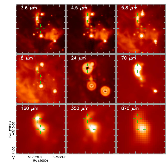
Figure 1.— IRAC 3.6, 4.5, 5.8, and 8.0 $\mu$m, MIPS 24 $\mu$m, PACS 70 and 160 $\mu$m, SABOCA 350 $\mu$m and LABOCA 870 $\mu$m images of the region around OMC-2 FIR 4 (SOF 3, HOPS 108). At 24 $\mu$m, the saturated sources to the north, south, and southwest are OMC-2 FIR 3 (SOF 2N, HOPS 370), OMC-2 FIR 5 (SOF 4, HOPS 369), and SOF 5 (HOPS 368), respectively. The two crosshairs show the position of FIR 3 (northern crosshairs) and FIR 4 (southern crosshairs).

In this section, we present our data on OMC-2 FIR 4 and explain how we extracted the photometry in the far-IR and sub-mm. OMC-2 FIR 4 was detected by the Spitzer InfraRed Array Camera (IRAC; Fazio et al., 2004) and Multiband Imaging Photometer for Spitzer (MIPS; Rieke et al., 2004) at 8.0 and 24 $\mu$m, respectively (Megeath et al. 2012; see Figure 1). A mid-infrared spectrum (5-37 $\mu$m) was also taken using the InfraRed Spectrograph (IRS; Houck et al., 2004) on Spitzer. FIR 4 was also detected at 37.1 $\mu$m using FORCAST (Herter et al., 2012) on SOFIA (source SOF 3 of Adams et al. 2012). As part of the Herschel Orion Protostar Survey (HOPS), a Herschel open-time key program (e.g., Fischer et al., 2010; Stanke et al., 2010; Stutz et al., 2013; Manoj et al., 2013, Fischer et al. 2014, in preparation; Ali et al. 2014, in preparation), it was observed with the Photodetector Array Camera and Spectrometer (PACS; Poglitsch et al., 2010) at 70 and 160 $\mu$m (see Figure 1). In the HOPS catalog, OMC-2 FIR 4 is source HOPS 108. It was also observed with PACS at 100 $\mu$m by the Gould Belt Survey (e.g., André et al., 2010). In the submillimeter, OMC 2 was mapped at 350 and 870 $\mu$m with the SABOCA and LABOCA instruments (Siringo et al., 2010, 2009, respectively) on the APEX telescope (see Figure 1). Table 1 displays the fluxes extracted from these data sets, as well as some measurements from the literature. Details on the data reduction and photometry for the PACS data can be found in Ali et al. (2014, in preparation), while details on the measurements of the APEX fluxes can be found in Stutz et al. (2013), Stutz et al. (2014, in preparation), and Stanke et al. (2014, in preparation).

Table 1Photometry of OMC-2 FIR 4

Wavelength	Flux [Jy]	Aperture radius	Reference
8 $\mu$m	0.03	2.4″	Megeath et al. (2012)
24 $\mu$m	1.519	PSF	Megeath et al. (2012)
37.1 $\mu$m	8.4	4.3″ beam	Adams et al. (2012)
70 $\mu$m	132.5	9.6″	this work
70 $\mu$m	40.81	PSF	this work
100 $\mu$m	287.7	9.6″	this work
160 $\mu$m	611.2	12.8″	this work
160 $\mu$m	270.2	PSF	this work
350 $\mu$m	67	12″ beam	Lis et al. (1998)
350 $\mu$m	54.7	7.34″	this work
350 $\mu$m	43.2	7.34″ beam	this work
850 $\mu$m	7.5	14″ beam	Johnstone & Bally (1999)
870 $\mu$m	12.3	19″	this work
870 $\mu$m	8.39	19″ beam	this work
1.3 mm	8.0	50″ $\times$ 50″	Mezger et al. (1990)
1.3 mm	1.252	22″ $\times$ 17″	Chini et al. (1997)
2.0 mm	1.06	4.87″ $\times$ 2.73″	López-Sepulcre et al. (2013)
3.6 cm	6.4 $\times 10^{-4}$	$\sim$ 8″ beam	Reipurth et al. (1999)

Note. — The flux values we use for our SED models are shown in bold (see text for details). In the column labeled “aperture radius”, “PSF” means that the flux was determined via PSF photometry, and a numerical value followed by “beam” indicates that the flux is the peak beam flux of the source as measured in a beam with the specified FWHM.

In the Spitzer IRAC images, OMC-2 FIR 4 is faint, but clearly detected, at 8.0 $\mu$m. Some emission can also be seen at 4.5 $\mu$m and 5.8 $\mu$m, but there is no well-defined point source at these wavelengths. At 5.8 $\mu$m, there seem to be two emission peaks, one that matches the 8 and 24 $\mu$m position, and one slightly offset, while at 4.5 $\mu$m there is a strong emission peak only at the offset position. The detection of emission offset relative to the peak position seen at 8-70 $\mu$m could be an indication of an outflow (see section V.4). About 6″ to the north of FIR 4 lies an object that is brighter in all IRAC bands, but much fainter at 24 $\mu$m and not detected at 70 $\mu$m and longer wavelengths (see Figure 1). This is source MIR 24 tentatively identified with FIR 4 by Nielbock et al. (2003), but it is a separate source (also known as HOPS 64 in the HOPS catalog).

The IRS spectrum of FIR 4 is very noisy in the 5-14 $\mu$m region, mostly due to deep ice and silicate absorption features, but at 8 $\mu$m agrees with the IRAC measurement within $\sim$20%. Given the slit widths of 3.6″ for the Short-Low module (SL; 5-14 $\mu$m) and 10.5″ for the Long-Low module (LL; 14-37 $\mu$m), as well as the slit orientations, none of the bright neighboring sources contaminated the IRS spectrum. Only HOPS 64, located 6.3″ to the north of FIR 4, partially entered the LL slit, but its flux contribution at wavelengths $\gtrsim$ 15 $\mu$m is small (its MIPS 24 $\mu$m flux is 0.57 Jy, compared to 1.5 Jy for FIR 4). There is a discrepancy between the MIPS 24 $\mu$m flux of FIR 4 and the 24 $\mu$m flux derived from IRS spectra in that the IRS flux is a factor of 2 too high. This could be due to the fact that more extended emission from the filament was included in the IRS measurement (slit width of 10.5″ compared to the typical FWHM of the MIPS 24 $\mu$m PSF of $\sim$ 6″). The IRS spectrum was scaled by 0.5 to match the MIPS 24 $\mu$m flux. When compared to the SOFIA/FORCAST measurement at 37.1 $\mu$m from Adams et al. (2012), where FIR 4 appears as a point source, the IRS spectrum is about a factor of 1.3-1.9 too high (the range considers the calibration uncertainty of the 37.1 $\mu$m flux), roughly consistent with the discrepancy found for the MIPS 24 $\mu$m flux.

At 70 and 160 $\mu$m, emission towards OMC-2 FIR 4 can be clearly discerned (Figure 1). FIR 4 is part of a dense filament extending from FIR 3 (HOPS 370) to the north. At 70 $\mu$m, a point source can be seen near the position of the Spitzer 8 and 24 $\mu$m source. To compare the position of the PACS sources to those in the Spitzer images, the PACS maps have been re-centered based on the average offsets between the Spitzer and PACS 70 $\mu$m observations of the HOPS targets in the field (see Figure 2). The offsets were determined independently for the four distinct images constructed from the four separate groups of PACS scans that covered FIR 4 as part of the HOPS program. In these four images, the 70 $\mu$m position of FIR 4 is offset from the Spitzer position by 0.4″ to 1.4″ (Figure 2), much smaller than the FWHM of 7″ at 70 $\mu$m. These offsets are comparable to the offsets found for the other HOPS sources in each group and match the positional uncertainty expected from the Herschel pointing accuracy of $\sim$ 2″. The offset between the Spitzer and PACS 70 $\mu$m data in right ascension is $\sim$ 0.7″-1″ larger for FIR 4 than the median offset for the other 70 $\mu$m sources in three of the four images; for the fourth image (constructed from group 135 scans), the offset for FIR 4 and the median offset agree within 0.2″. However, in each group there are other objects with similar right ascension offsets as FIR 4, so it is not exceptional. Thus, we conclude that the Spitzer 8, 24 and 70 $\mu$m objects are coincident to within the accuracy of our data.

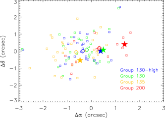
Figure 2.— Offsets in right ascension and declination relative to the Spitzer positions for all PACS 70 $\mu$m sources with Spitzer analogs in the fields that contain the source OMC-2 FIR 4. The targets were observed by Herschel in four different scan groups, represented by four colors. The squares identify all HOPS targets observed in these groups, with FIR 4 shown with a filled star symbol. The open diamonds represent the median offsets found for the objects in the four groups.

Similarly, the 160 $\mu$m map was corrected using the offsets derived from the 70 $\mu$m observations, given that it was observed at the same time. There is an offset between the 70 $\mu$m source and the peak of the 160 $\mu$m emission: the brightest part of the extended emission is about 3″ to the northwest of the mid-IR (and 70 $\mu$m) position of FIR 4. This 160 $\mu$m peak also overlaps in position with the peak seen at 350 and 870 $\mu$m, suggesting that, as opposed to the “warm” ($\leq$ 70 $\mu$m) peak resulting from envelope emission, the “cold” peak could arise from externally heated dust (see section V.5). Although there is a clear peak in the $\lambda$ $\geq$ 160 $\mu$m emission towards FIR4, the source in these bands is markedly extended and is not a point source.

We carried out aperture photometry at 70 and 160 $\mu$m by centering on the peak of the emission in each band. With aperture photometry at 70 $\mu$m using an aperture radius of 9.6″, a sky annulus of 9.6″-19.2″, and an aperture correction factor of 1.364, we derived a flux of 132.5 Jy (the sky emission, i.e., the mode of fluxes inside the sky annulus, amounted to just 0.1 Jy). However, when applying PSF photometry, we derived 40.8 $\pm$ 4.7 Jy (see Ali et al. 2014, in preparation, for details). It is clear that aperture photometry includes a large contribution of the extended, filamentary emission around FIR 4, so PSF photometry should yield a more reliable source flux at 70 $\mu$m. The residual images from the PSF fits indicated that only a small amount of extended emission was left around the position of FIR 4. Thus, the flux value from PSF photometry might underestimate the true emission from the protostar at 70 $\mu$m, but not by much.

The PACS 160 $\mu$m flux is similarly affected by extended emission. FIR 4 is brighter than its northern neighbor FIR 3, but it is embedded in the filament connecting both. Aperture photometry at 160 $\mu$m, centered on the brightness peak at 160 $\mu$m, with an aperture radius of 12.8″, sky annulus of 12.8″-25.6″, and an aperture correction factor of 1.515, yielded a flux of 611.2 Jy (once again, the sky emission was low, just 1.3 Jy). On the other hand, PSF photometry resulted in 270.2 $\pm$ 8.4 Jy. This flux is a slightly better estimate of the envelope emission at 160 $\mu$m, but given that there is no distinct point source at this wavelength, it probably still has a large contribution from extended emission. Also, the positional offset between the 70 and 160 $\mu$m peak indicated that it is possible that the main contribution to the 160 $\mu$m emission stems from externally heated dust in a massive core that encompasses the protostar (see section V.5), and thus the emission from the envelope itself could be very small. For the PACS 100 $\mu$m flux, we only had aperture photometry available; adopting the same aperture radius and sky annulus as for the 70 $\mu$m data, and an aperture correction factor of 1.440, we derived 287.7 Jy for the flux at 100 $\mu$m. Since this value very likely overestimates the intrinsic flux from FIR 4, we treat it as an upper limit.

The morphology of OMC-2 FIR 4 is similar at 160 and 350 $\mu$m (Figure 1). It is the brightest object in the area, but embedded in extended emission. To derive a SABOCA 350 $\mu$m flux for this object, we adopted its beam flux of 43.2 Jy (the SABOCA beam has a FWHM of 7.34″), with the centroid determined within a box of size 1.65 $\times$ FWHM around the Spitzer position to account for potential offsets. Thus, the beam flux was centered at the brightness peak of the 350 $\mu$m emission from FIR 4. Aperture photometry with a radius of 3.67″ (and no sky subtraction) yielded 29.3 Jy; aperture photometry adopting a radius of 7.34″ and a sky annulus of 11.0″-14.7″ resulted in 54.7 Jy.

At 870 $\mu$m, FIR 4 is clearly the brightest object, but it is also extended (Figure 1). The LABOCA 870 $\mu$m beam flux (beam FWHM of 19″) amounted to 8.4 Jy; also at 870 $\mu$m, the centroid position of the source was determined separately, with the Spitzer position as starting point. Aperture photometry using a radius half the FWHM and no sky subtraction yielded 5.1 Jy, while aperture photometry within a radius of 19″ and sky annulus of 28.5″-38″ resulted in 12.3 Jy. Adams et al. (2012) reported similar SABOCA and LABOCA beam fluxes for FIR 4.

III. Spectral Energy Distribution and Bolometric Luminosity

Figure 3 shows the SED of OMC-2 FIR 4 constructed with the data mentioned in the previous section. As discussed earlier, the IRS spectrum displays deep ice absorption features in the 5-8 $\mu$m region (due to water ice, methanol, and other organic species), and its silicate absorption feature centered at 10 $\mu$m is also very deep (with no detected flux over the wavelength interval of maximum absorption). The CO₂ ice feature at 15.2 $\mu$m is, in comparison, less pronounced. The change in slope in the spectrum beyond about 30 $\mu$m is very likely due to a strong water ice absorption, which is fairly broad and centered at $\sim$ 45 $\mu$m. The SED plot also shows the fluxes derived from aperture photometry for PACS, SABOCA, and LABOCA data. The difference between aperture and PSF photometry is quite large for PACS fluxes (factors of 3.2 and 2.3 at 70 and 160 $\mu$m, respectively), but smaller at 350 and 870 $\mu$m (factors of 1.3 and 1.5, respectively).

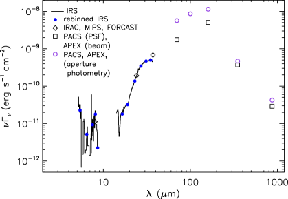
Figure 3.— SED of OMC-2 FIR 4 using Spitzer IRAC, IRS, and MIPS, SOFIA/FORCAST, Herschel PACS, and APEX SABOCA and LABOCA data. The small blue dots on the IRS spectrum show the data points that are used in the calculation of $L_{bol}$ and $T_{bol}$ and for the model fits. The black diamonds at 8, 24, and 37 µm represent the IRAC, MIPS, and FORCAST photometry, respectively. The black squares at 70 and 160 µm represent PACS PSF photometry measurements, while the open, purple circles at these wavelengths and at 100 $\mu$m represent values from aperture photometry. The black squares at 350 and 870 µm represent SABOCA and LABOCA beam fluxes, while the open, purple circles at these wavelengths represent aperture photometry values using radii equal to the FWHM of the beams and sky subtraction (see text for details).

As mentioned in section II, there seems to be a $\sim$ 3″ offset in the position of the emission peak between data at 8-70 $\mu$m and $\gtrsim$ 160 $\mu$m. When deriving fluxes using aperture photometry, we re-centered at the peak position in each wave band (this is standard procedure for all our targets in the HOPS sample); thus, at longer wavelengths, the aperture was not centered at the same position as was used for the fluxes below 100 $\mu$m. If the far-IR and sub-mm emission is dominated by an externally heated clump of molecular material (which is likely the case; see section V.5), then our 100, 160, 350, and 870 $\mu$m fluxes overestimate the emission from the protostar itself and should rather be taken as upper limits. However, using these fluxes gives an idea of the maximum luminosity that could possibly be associated with the protostar OMC-2 FIR 4.

To calculate the bolometric luminosity ($L_{bol}$) from the observed SED, we first rebinned the IRS spectrum to exclude those parts of the spectrum dominated by ices and to smooth over noisy regions (see Figure 3). This resulted in flux values at 5.4, 6.45, 7.5, 8.1, 8.6, 16.5, 19.0, 23.0, 27.0, 31.0, and 35.0 $\mu$m that trace the continuum emission and part of the short-wavelength wing of the broad silicate absorption feature centered around 10 $\mu$m. If we use the measured Spitzer IRAC and MIPS photometry, the rebinned version of the IRS spectrum, PSF photometry at 70 and 160 $\mu$m, and the beam fluxes at 350 and 870 $\mu$m, we derive a bolometric luminosity of just 36.6 $L_{\odot}$. The corresponding bolometric temperature ($T_{bol}$) is 34.1 K. Neither interpolation of fluxes between the sampled values nor extrapolation of fluxes at wavelengths below 5.4 $\mu$m and beyond 870 $\mu$m was done. However, even when we extrapolated the long-wavelength fluxes out to 10 mm using a power law $F_{\nu}\propto{\nu}^{2}$, we derived the same $L_{bol}$ value and a $T_{bol}$ value that is nearly identical, 34.0 K. Since the fluxes in the near-infrared are very small, likely much less than 10 mJy, they would not affect the resulting $L_{bol}$ value.

Table 2Bolometric Luminosity of OMC-2 FIR 4

	Data used for $L_{bol}$ calculation
$L_{bol}$ [$L_{\odot}$]	IRAC	MIPS	IRS	70 $\mu$m	100 $\mu$m	160 $\mu$m	350 $\mu$m	870 $\mu$m
36.6	aper	PSF	yes	PSF	no	PSF	beam	beam
40.7	aper	PSF	no	PSF	no	PSF	beam	beam
78.8	aper	PSF	yes	aper	aper	aper	beam	beam
86.0	aper	PSF	yes	aper	aper	aper	aper	aper
100.2	aper	PSF	no	aper	aper	aper	aper	aper

Note. — “PSF” means that the flux was determined via PSF photometry, “aper” means that the flux was measured with aperture photometry, including subtraction of a sky value determined in a sky annulus. “no” means that these data were not included in the $L_{bol}$ calculation. Our preferred $L_{bol}$ determination is shown in bold.

If we exclude the IRS spectrum from the calculation, we get 40.7 $L_{\odot}$ for $L_{bol}$ and 36.5 K for $T_{bol}$. In this case $L_{bol}$ is slightly higher, since the interpolated area under the SED is somewhat larger without the IRS spectrum. If we use the mid-IR photometry, IRS spectrum, sub-mm beam fluxes, but adopt aperture photometry at PACS wavelengths (including the 100 $\mu$m data point), we calculate 78.8 $L_{\odot}$ for $L_{bol}$ and 36.6 K for $T_{bol}$. Finally, adopting aperture photometry at both PACS and APEX wavelengths (with the latter using the aperture radius equal to the FWHM of the beam and sky subtraction), we derive $L_{bol}$=86.0 $L_{\odot}$ and $T_{bol}$=33.8 K (these values change to 100.2 $L_{\odot}$ and 36.7 K, respectively, if the IRS spectrum is excluded). Our $L_{bol}$ calculations are summarized in Table 2.

Thus, depending on which measurements are adopted, we derive bolometric luminosities ranging from 37 $L_{\odot}$ to 100 $L_{\odot}$ for OMC-2 FIR 4. This large range is simply a result of the complex region around this protostar. However, given that emission from the cold, externally heated clump appears to dominate the fluxes at $\lambda>$ 160 $\mu$m (see section V.5), the $L_{bol}$ value most closely characterizing the protostar is 37 $L_{\odot}$. In contrast, the $T_{bol}$ value shows little dependence on the chosen photometry, ranging from 34 to 37 K.

IV. Fits of the SED with Standard Protostar Models

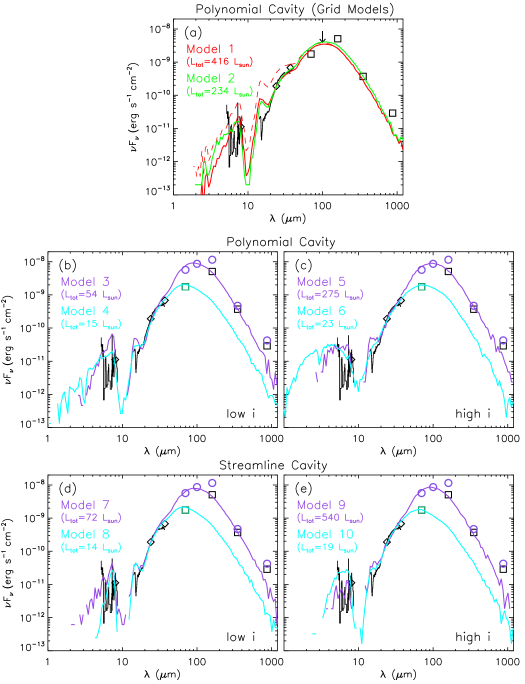
Figure 4.— SED of OMC-2 FIR 4 from Figure 3, shown with ten different model fits (the lines representing the models use fluxes from three apertures: 4″ for $\lambda<8\,\mu$m, 5″ for $\lambda=$ 8-37 $\mu$m, and 10″ for $\lambda>37\,\mu$m). (a) Best-fit model from the model grid from Furlan et al. (2014, in preparation), which uses polynomial-shaped cavities (Model 1, red solid line; the dashed line shows this same model, but with $A_{V}$ set to 0); best-fit model from the model grid with $A_{V}$=0 (Model 2, green line). (b) and (c) Model fits using polynomial-shaped cavities, one set for low and one set for high inclination angles: fits to the far-IR and sub-mm aperture photometry values, shown with the open circles (Models 3 and 5, purple lines); fits focusing only on the mid-infrared data and the PACS 70 $\mu$m PSF photometry value, shown as the green square (Models 4 and 6, cyan lines). (d) and (e) Similar to (b) and (c), but using models with streamline-shaped cavities. See text for details and Table 3 for model parameters.

Adams et al. (2012) modeled the SED of OMC-2 FIR 4 using IRAC 8.0 $\mu$m, MIPS 24 $\mu$m, SOFIA/FORCAST 37.1 $\mu$m, PACS 70 and 160 $\mu$m, and APEX 350 and 870 $\mu$m data. Their reported PACS and APEX fluxes were extracted from an earlier version of the reduced maps. They adopted the sheet collapse model for the envelope from Hartmann et al. (1996) and included the accretion disk model from D’Alessio et al. (1999, 2006). The outflow cavities in the envelope were assumed to follow the streamlines of infalling particles. Depending on whether they included the 160 $\mu$m data point as upper limit, they obtained a total intrinsic luminosity of 50 $L_{\odot}$ (30 $L_{\odot}$ with an upper limit at 160 $\mu$m), an inclination angle of 50° (70°), a cavity opening angle of 8°, an envelope radius of 5000 AU, an envelope reference density $\rho_{1}$ (see Kenyon, Calvet, & Hartmann, 1993) of 20 (5) $\times 10^{-13}$ g cm^-3, and an envelope mass of 10 (2.5) $M_{\odot}$.

In Furlan et al. (2014, in preparation), we used models from a grid developed for the HOPS program to find the best-fit model of OMC-2 FIR 4 based on an $R$ statistic (Fischer et al., 2012). These models were calculated using the Monte Carlo radiative transfer code developed by Whitney et al. (2003a, b). They use the solution of a rotating, infalling cloud core from Terebey, Shu, & Cassen (1984); the disk embedded in the envelope is described by a density power law and a flaring angle exponent. The dust opacities were adopted from Ormel et al. (2011), which include larger, icy grains. As opposed to Adams et al. (2012), the cavity carved out in the envelope by the outflows was assumed to have a power law shape (exponent of 1.5; Whitney et al. 2003a), not conical as in the case of a streamline cavity.

Table 3Models for OMC-2 FIR 4

				Parameters
Model	$L_{tot}$	$R_{disk}$	$\rho_{1}$	$\rho_{1000}$	cavity	$\theta$	$i$	$A_{V}$	$R$	$L_{bol}$	$T_{bol}$
	[$L_{\odot}$]	[AU]	[g cm-3]	[g cm-3]		[°]	[°]	[mag]		[$L_{\odot}$]	[K]
Model 1	416	100	7.5 $\times$ 10-13	2.4 $\times$ 10-17	poly	45	70	23.9	3.81	25	43
Model 2	234	500	1.9 $\times$ 10-12	5.9 $\times$ 10-17	poly	45	63	0.0	4.03	30	41
Model 3	54	500	5.6 $\times$ 10-13	1.8 $\times$ 10-17	poly	5	32	0.0	6.02	58	43
Model 4	15	10	1.1 $\times$ 10-13	3.3 $\times$ 10-18	poly	5	49	0.0	3.03	14	57
Model 5	275	500	8.3 $\times$ 10-13	2.6 $\times$ 10-17	poly	35	63	0.0	4.01	59	42
Model 6	23	500	7.5 $\times$ 10-14	2.4 $\times$ 10-18	poly	10	70	0.0	3.04	14	56
Model 7	72	500	7.5 $\times$ 10-13	2.4 $\times$ 10-17	stream	25	32	0.0	4.32	52	43
Model 8	14	10	9.8 $\times$ 10-14	3.1 $\times$ 10-18	stream	5	49	0.0	4.41	14	59
Model 9	540	500	6.0 $\times$ 10-13	1.9 $\times$ 10-17	stream	50	63	0.0	8.34	53	43
Model 10	19	50	7.5 $\times$ 10-14	2.4 $\times$ 10-18	stream	15	87	0.0	2.85	12	60

Note. — The model parameters are as follows: $L_{tot}$ is the total luminosity (which is the sum of the stellar and accretion luminosity), $R_{disk}$ the disk radius (which is equal to the centrifugal radius), $\rho_{1}$ and $\rho_{1000}$ are the reference density at 1 and 1000 AU, respectively, $\theta$ is the cavity opening angle, $i$ the inclination angle, $A_{V}$ the foreground extinction along the line of sight, and $R$ is a measure for the goodness-of-fit. The column labeled “cavity” describes the cavity shape: “poly” for polynomial, “stream” for streamline. For a polynomial-shaped cavity, the cavity shape exponent is 1.5. The $L_{bol}$ and $T_{bol}$ values were measured by using the fluxes of the individual model SEDs. Note that for all models the stellar radius is 6.61 $R_{\odot}$, the stellar luminosity 10.0 $L_{\odot}$, the stellar mass 0.5 $M_{\odot}$, the disk mass 0.05 $M_{\odot}$, the disk scale height exponent 1.25, and the disk density exponent 2.25. The outer envelope radius is set to 10,000 AU. Models in italics are those that, at longer wavelengths, fit aperture photometry at 70, 100, 160, 350, and 870 $\mu$m, while the other models fit the PSF photometry value at 70 $\mu$m (and, in the case of Models 1 and 2, also PSF photometry at 160 $\mu$m and the beam fluxes at 350 and 870 $\mu$m).

For the SED fit in Furlan et al. (2014, in preparation), we used the IRAC, MIPS, rebinned IRS fluxes (as described in section III), the fluxes from PSF photometry at 70 and 160 $\mu$m, and the beam fluxes at 350 and 870 $\mu$m. The best-fit model from the grid resulted in a total intrinsic luminosity $L_{tot}$ of 416 $L_{\odot}$, an inclination angle of 70°, a cavity opening angle of 45°, and an envelope reference density $\rho_{1}$ of 7.5 $\times 10^{-13}$ g cm^-3 (see Model 1 in Figure 4 (a) and Table 3). This model also required a substantial foreground extinction of $A_{V}=23.9$. However, the next-best model from the grid resulted in no foreground extinction, a somewhat lower inclination angle ($i=$63°), $L_{tot}$ of 234 $L_{\odot}$, the same cavity opening angle, and a $\rho_{1}$ value of 1.9 $\times 10^{-12}$ g cm^-3 (see Model 2 in Figure 4 (a) and Table 3). Thus, the total luminosity of the source derived from models strongly depends on the amount of assumed foreground extinction; with an $A_{V}$ value of 23.9 as opposed to 0, the total luminosity changed by almost a factor of two.

We also ran new model calculations using the same Monte Carlo code of Whitney et al. (2003a, b) for a more in-depth exploration of the parameter space. As a starting point for our input files with the model parameters, we used the files from the HOPS model grid; thus, many parameters that we did not adjust, such as the stellar mass and disk density exponent, are the same. We first used a polynomial-shaped cavity, as in our model grid, then a streamline-shaped cavity, since the cavity shape can have a large effect on the resulting model SED (especially if the cavity opening angle is large), but for FIR 4 is not constrained by observations. Similarly, the inclination angle is not constrained, so we explored two sets of models, one with lower inclination angles and one with a more edge-on orientation. We also assumed no foreground extinction; substantial extinction along the line of sight would result in higher total luminosities and change other model parameters, in particular the inclination angle, given that extinction affects mostly the near- and mid-infrared fluxes (see Figure 4 (a)).

In panels (b) and (c) of Figure 4, we show the model fits assuming a polynomial-shaped cavity for more face-on and more inclined models, respectively. Each panel shows two model fits each, one that considers the long-wavelength aperture photometry (purple lines), and one that only tries to fit the mid-infrared data and the PSF photometry value at 70 $\mu$m (cyan lines). As can be seen from Table 3 (Models 3-6) the total luminosity varies widely, depending on which data points are modeled and which orientation along the line of sight is assumed. Models that take aperture photometry at 70 $\mu$m and beyond into account (Models 3 and 5) have higher $L_{tot}$ values and higher envelope densities than models that consider only the 70 $\mu$m PSF photometry value at long wavelengths (Models 4 and 6). Also, more edge-on models require total luminosities that are larger than those for models with $i$ $\sim$ 30°-50°. These high-inclination models also have larger cavity opening angles. The reference density for models fitting the same data sets changes by about 50% between the two sets of inclination angles.

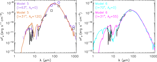
Figure 5.— SED of OMC-2 FIR 4 with model 5 (left panel) and model 6 (right panel). In each panel, the same model is first shown with the best-fit inclination angle and $A_{V}$=0 (purple and cyan lines), then with a low inclination angle and a relatively high foreground extinction (orange and magenta lines).

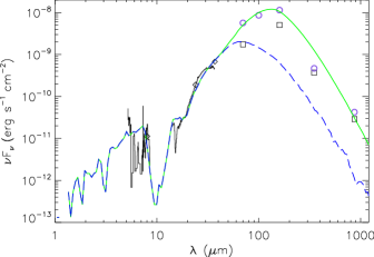
Figure 6.— SED of OMC-2 FIR 4 as in Figure 4 (b)-(e) shown with a model composed of Model 4 (blue dashed line; see also Figure 4 (b)) and a modified blackbody with a temperature of 18.5 K; the combined fluxes are shown with the green solid line.

A similar result applies to the four models that assume a streamline-shaped cavity (Figure 4 (d) and (e), Models 7-10 in Table 3). Compared to the models with polynomial-shaped cavities, the models fitting fluxes from aperture photometry at long wavelengths (Models 7 and 9 vs. Models 3 and 5) have larger $L_{tot}$ values and cavity opening angles, while these parameters are quite similar for the models fitting just the mid-infrared fluxes and the flux from PSF photometry at 70 $\mu$m (Models 8 and 10 vs. Models 4 and 6). Thus, to reproduce large flux values in the far-IR and a steeply rising SED in the mid-IR, a model with a streamline-shaped cavity requires a larger cavity opening angle and a much higher total luminosity than models with polynomial-shaped cavities. This latter type of cavity evacuates more material in the inner envelope than a streamline-shaped cavity, and as a result more shorter-wavelength photons can reach the observer. In the extreme case of Model 9, where $L_{tot}=$ 540 $L_{\odot}$ is required, the streamline-shaped cavity also has to have an opening angle of 50° such that sufficient infrared flux escapes from the envelope. Interestingly, the models with the streamline-shaped cavity have envelope densities similar to those of the models with the polynomial-shaped cavity. The higher-luminosity models still require envelopes denser by up to an order of magnitude.

For each of the models, Table 3 lists their $R$ value, which is a measure for the goodness-of-fit introduced by Fischer et al. (2012) (see also Furlan et al. 2014, in preparation). $R$ is defined as follows: $R=\frac{1}{N}\sum_{i=1}^{N}w_{i}|\ln(F_{obs}(\lambda_{i})-\ln(F_{mod}(\lambda_{i})|,$ where $w_{i}$ is the weight for each data point, $F_{obs}$ and $F_{mod}$ are the observed and model fluxes, respectively, and the sum is over the number of data points. The weights were set to the inverse of the approximate fractional uncertainty of each flux measurement and ranged from 1/0.04 to 1/0.4 (with more weight given to the 3-70 $\mu$m region; see Furlan et al. 2014, in preparation, for details). When calculating $R$ values for the various models, we used the same photometry values and rebinned IRS fluxes (see Figure 3 and section III) in the mid-IR, but at longer wavelengths we included aperture photometry at $\lambda\geq$ 70 $\mu$m for models 3, 5, 7, and 9, and only the 70 $\mu$m PSF photometry at 70 $\mu$m for models 4, 6, 8, and 10. Thus, the $R$ values for the latter set of models are in general lower than those for the former set. Overall, most models have $R$ values in the 3-4 range; from a visual inspection of Figure 4, they are indeed quite comparable, with the most noticeable differences in the near-IR and in the depth of the 10 $\mu$m silicate feature, where there is little to no emission in both the observed and modeled fluxes (and thus they do not have a measurable effect on the $R$ value).

So far, the models calculated for this work do not include any foreground extinction. As mentioned earlier and shown in Figure 4 (a), extinction will depress the near- and mid-IR fluxes and leave the far-IR and sub-mm fluxes unchanged. Thus, its effect is similar to that of the inclination angle; dust in a highly inclined envelope will cause more extinction of photons on their way to the observer. In Figure 5 we explored the effect of foreground extinction on two of the high-inclination models (Models 5 and 6). They are shown with their best-fit inclination angle (63° and 70°, respectively) and no additional extinction along the line of sight, and with a low inclination angle of 31° and foreground extinction large enough such that the model fluxes still roughly reproduce the observed SED. With a low inclination angle, model 5 requires $A_{V}$=120, while model 6 needs $A_{V}$=55. Even though these latter models could benefit from tweaking some parameters, they demonstrate that inclination angle and foreground extinction are highly degenerate parameters. Thus, our models with high luminosity either require a large foreground extinction or a more edge-on orientation.

To examine the effect of a significant contribution from extended, externally heated emission to the far-infrared and submillimeter fluxes, we used a model that fits the mid-infrared data points and the PSF photometry at 70 $\mu$m and added a modified blackbody (for the latter, we used the same dust opacities from Ormel et al. (2011) adopted for our models). All the other models presented so far do not include such a component; the long-wavelength fluxes are just fit by emission from the disk and envelope. We chose Model 4 to represent the protostar, but since Models 4, 6, 8, and 10 all have similar SEDs in the 20-1000 $\mu$m range and $L_{bol}$ values of 12-14 $L_{\odot}$, the choice of model does not affect the results. With the combined protostar and blackbody model, we aimed to fit the aperture photometry fluxes at long wavelengths, since they are most likely dominated by extended emission. The best-fit combination of Model 4 and a modified blackbody is shown in Figure 6; it requires a blackbody temperature of 18.5 K. The PACS 70, 100, and 160 $\mu$m fluxes are fit well, while the 350 $\mu$m flux is overestimated and the 870 $\mu$m flux slightly underestimated. The discrepancy at 350 $\mu$m is likely an aperture effect, given the small aperture used at this wavelength. The combined bolometric luminosity of Model 4 and the 18.5 K blackbody amounts to 76 $L_{\odot}$, which is very similar to the $L_{bol}$ value measured from the observed SED with the mid-IR data, aperture photometry at 70, 100, and 160 $\mu$m, and the beam fluxes in the sub-mm (see section III). The contribution of the modified blackbody to this $L_{bol}$ value is 62 $L_{\odot}$, leaving just 14 $L_{\odot}$ as $L_{bol}$ for the protostar.

V. Discussion

V.1. The Bolometric Luminosity of the Protostar OMC-2 FIR 4

Our new measurements of OMC-2 FIR 4 in the far-IR and submillimeter suggest that its bolometric luminosity is far below the most recent value of $\sim$ 1000 $L_{\odot}$ suggested in the literature: we derive a range from 37 $L_{\odot}$ to $\sim$ 100 $L_{\odot}$, with the former value more likely to describe the protostar, since it is derived using smaller apertures for the source fluxes. Also, given that the IRS spectrum plays an important role in constraining the mid-infrared part of the SED, the more realistic upper limit for $L_{bol}$ is 86 $L_{\odot}$ (which is derived when including the IRS spectrum in the SED).

As noted by López-Sepulcre et al. (2013), the fluxes and thus luminosity of OMC-2 FIR 4 depend strongly on which apertures are used. The larger the aperture, the more envelope emission, but also extended emission from the surrounding filament and emission from neighboring sources is included. We find that, for isolated protostars in the Orion star-forming region (distance of $\sim$ 420 pc; Menten et al. 2007; Hirota et al. 2007), aperture radii of $\sim$ 10″ in the far-IR (70-160 $\mu$m) capture most of the emission from the envelope at these wavelengths (see Furlan et al. 2014, in preparation). Choosing larger radii risks including surrounding emission that is not associated with the envelope. Crimier et al. (2009) likely overestimated the fluxes of FIR 4, since they integrated their derived continuum profiles at 350, 450, and 850 $\mu$m out to $\sim$ 20″, their derived envelope size. However, FIR 4 seems to be surrounded by extended emission, and a 20″ aperture will include emission from this surrounding material. Their derived fluxes at 350 and 850 $\mu$m are about an order of magnitude larger than our APEX fluxes at similar wavelengths. Crimier et al. (2009) also extracted IRAS fluxes at 60 and 100 $\mu$m; however, the IRAS beam is very large at these wavelengths, and contamination by FIR 3 and FIR 5 likely also plays a role. Their extracted MIPS 24 $\mu$m flux is also overestimated due to the aperture radius of 15″; their flux value of 5.0 Jy is 3.3 times larger than the value derived by Megeath et al. (2012) with PSF fitting.

The big discrepancy in flux measurements resulting from adopting apertures that are at most a factor of a few different suggests that the region around FIR 4 is very complex and contains copious amounts of extended emission. The dust in this extended material is likely to be heated by the strong far-IR radiation field present in the Orion cloud complex, and is not internally heated by the protostar itself. Thus, if we want to characterize the protostar itself, it seems reasonable to adopt conservative (i.e., smaller) aperture sizes to measure fluxes. The offset we found for the emission peak at $\lambda$ $\leq$ 70 $\mu$m and $\lambda$ $\geq$ 160 $\mu$m suggests that even our lowest flux values in the 160-870 $\mu$m region could overestimate the envelope emission. This is supported by the interferometer results of López-Sepulcre et al. (2013), who found that there are multiple components in OMC-2 FIR 4, only one of which contains a protostar. We therefore ignore the more extended core resolved in the observations of Shimajiri et al. (2008) and López-Sepulcre et al. (2013) and focus on the properties of the protostar and its inner ($\lesssim$ 8,000 AU radius) envelope. As shown in section IV, protostellar models that assume a dense, infalling envelope around a single protostar can describe the observed SED. We will discuss the relationship of this protostar to the more extended core in the FIR 4 region in section V.5.

V.2. The Classification of the Protostar OMC-2 FIR 4

Adopting an $L_{bol}$ value of 37 $L_{\odot}$ for FIR 4, and using the beam fluxes at 350 and 870 $\mu$m, we can calculate the ratio of sub-mm luminosity ($L_{submm}$) and $L_{bol}$. For $L_{submm}$, we integrated the SED at wavelengths $\geq$ 350 $\mu$m (André et al., 1993). We derived $L_{submm}$/$L_{bol}$ of 2% (the result is the same if we add a long-wavelength extrapolation to the SED reaching to 10 mm). This value is four times larger than the minimum value for a Class 0 protostar (André et al., 1993), so OMC-2 FIR 4 appears to be in a very early, evolutionary state, when presumably most of the stellar mass is still in the envelope or core surrounding the protostar. Thus, it shares some of the properties of the PACS Bright Red sources (PBRs) discovered by Stutz et al. (2013), which are among the youngest protostars, with high envelope densities and infall rates. The log of the ratio of its 70 and 24 $\mu$m flux in $\lambda F_{\lambda}$ space amounts to 0.96, while for PBRs this ratio is larger than 1.65. Nonetheless, our model fits (section IV) yielded high envelope densities, $\rho_{1}$ $\geq$ 7.5 $\times$ 10^-14 g cm^-3, very similar to those of the PBRs studied in Stutz et al. (2013).

Even model fits that at longer wavelengths only included the 70 $\mu$m PSF photometry point (Models 4, 6, 8, and 10) resulted in $\rho_{1}$ values close to 1.0 $\times$ 10^-13 g cm^-3, suggesting that even if we assume that the far-IR and sub-mm emission is dominated by externally heated dust, the derived envelope density of FIR 4 is still large. These models also yielded $L_{bol}$ values of 12-14 $L_{\odot}$ for the protostar, which is less than half the smallest value measured from the observed SED, but is a result of these model fluxes being lower by almost a factor of 10 compared to the beam fluxes at 350 and 870 $\mu$m and the flux from PSF photometry at 160 $\mu$m (see Figure 4). The ratios of sub-mm to bolometric luminosity for these models is 0.5-0.6%, on the low end for a Class 0 object (André et al., 1993), but the $T_{bol}$ values are $\leq$ 60 K and thus clearly in the Class 0 range (Chen et al., 1995). Therefore, there is strong observational evidence that OMC-2 FIR 4 is a Class 0 protostar. The high envelope density suggests that it is in an early evolutionary stage, and its SED classification as a Class 0 object translates into a Stage 0 physical state (see Robitaille et al., 2006).

V.3. Determining Source Properties from Models

As shown in section IV, a wide range of models can fit the observed fluxes of OMC-2 FIR 4, especially due to the somewhat uncertain source fluxes in the far-infrared and submillimeter and unconstrained model parameters such as the inclination angle and cavity shape. On the other hand, the current model fits can already give rough estimates for some source properties: the envelope density is relatively high, in the $\rho_{1}$ $\sim$ 10^-13 $-$ 10^-12 g cm^-3 (or $\rho_{1000}$ $\sim$ 3 $\times$ 10^-18 $-$ 3 $\times$ 10^-17 g cm^-3) range, and the cavity is either relatively narrow, combined with a more face-on orientation, or wide, if the inclination angle is high or a large amount of foreground extinction is present.

When comparing our models 7 and 9 to the modeling results of Adams et al. (2012), the envelope reference densities are similar, but our total luminosities and cavity opening angles are larger. Even though all these models assume streamline-shaped cavities, Adams et al. (2012) used the sheet collapse solution for the envelope structure. This results in a wider region of decreased density along the rotation axis (which is the same as the outflow axis) compared to our TSC models, roughly corresponding to a wider cavity. Thus, a sheet-collapse model with a smaller cavity still allows the escape of a large amount of mid-IR photons, even at higher inclination angles. Our models require both higher total luminosities (by up to a factor of $\sim$ 20) and larger cavity opening angles (by up to a factor of 6) to allow sufficient photons to reach the observer.

Inferring the total luminosity for FIR 4 is more difficult. While the bolometric luminosity is derived from the observed SED (assuming isotropic emission), the total luminosity is the intrinsic energy output from the object. Depending on the inclination angle, cavity opening angle, or the amount of foreground extinction, an object with the same $L_{tot}$ value will have $L_{bol}$ values that are higher or lower (see Whitney et al., 2003a). Observed fluxes determine $L_{bol}$, so it is not straightforward to convert it to an L_tot value. With $A_{V}=23.9$, $L_{tot}$ of FIR 4 can be as high as 416 $L_{\odot}$, but also a model with a streamline-shaped cavity, $A_{V}=0$, and a more edge-on orientation can yield $L_{tot}=$ 540 $L_{\odot}$. On the other hand, the $L_{bol}$ value derived from these two model SEDs is 25 $L_{\odot}$ for the former model and 53 $L_{\odot}$ for the latter one (see Table 3).

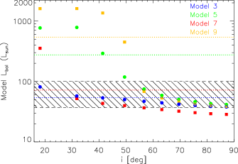
Figure 7.— The bolometric luminosity versus the inclination angle for Models 3 (blue; $L_{tot}$=54 $L_{\odot}$), 5 (green; $L_{tot}$=275 $L_{\odot}$), 7 (red; $L_{tot}$=72 $L_{\odot}$), and 9 (yellow; $L_{tot}$=540 $L_{\odot}$). The horizontal, dotted lines show the value of $L_{tot}$ for these four models. The dashed region shows the range of $L_{bol}$ values derived from the observed SED of OMC-2 FIR 4 (see text for details).

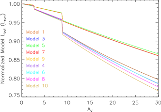
Figure 8.— The bolometric luminosity, obtained after the fluxes were attenuated by extinction and normalized to the $L_{bol}$ value at $A_{V}$=0, versus the foreground extinction $A_{V}$ for Models 1 (orange), 3 (blue), 5 (green), 7 (red), and 9 (yellow), 4 (purple), 6 (cyan), 8 (magenta), and 10 (beige). The discontinuities at $A_{V}$ values of 2.7 and 9 are due to the transitions to different extinction laws (Mathis 1990 $R_{V}$=5 curve for $A_{V}$=0-2.7, and two curves from McClure 2009 for $A_{V}$=2.7-9 and 9-30).

In Figure 7, we show the effect of inclination angle on $L_{bol}$ derived for the fluxes of those models that aim at fitting the aperture photometry values at longer wavelengths (Models 3, 5, 7, and 9). Each model has a certain total luminosity, $L_{tot}$ (see Table 3), which does not depend on the inclination angle. However, $L_{bol}$, which is derived from the SED, strongly depends on the viewing angle (see Whitney et al., 2003a, section 3.3). For more face-on orientations, $L_{bol}$ is higher than $L_{tot}$, especially for the higher-luminosity models. At $i\gtrsim$ 45°, the bolometric luminosity is lower than $L_{tot}$. Thus, to fit the observed $L_{bol}$ values, a high-luminosity model requires a larger inclination angle than a model with a lower total luminosity. This is reflected in the results presented in Table 3, where the models with the highest luminosity have inclination angles $\geq$ 63°. Given that $L_{bol}$ of FIR 4 is likely $\sim$ 40 $L_{\odot}$ based on the observations (see section III), a total luminosity of a few hundred $L_{\odot}$ is only possible if the inclination angle of the object is relatively high.

The effect of foreground extinction on $L_{bol}$ is less dramatic than that of the inclination angle, as long as $A_{V}\lesssim$ 30 (see Figure 8). Using all the models from Table 3 except for Model 2, we calculated $L_{bol}$ for $A_{V}=$ 0-30 (i.e., we extinguished the fluxes using $A_{V}$ values ranging from 0 to 30, then computed $L_{bol}$) and plotted $L_{bol}$ normalized by its value at $A_{V}$=0. Models 3, 5, 7, and 9 (which aimed at fitting the higher far-IR and sub-mm flux values) show a nearly identical decline in $L_{bol}$ with increasing extinction; at $A_{V}$=30, $L_{bol}$ is 86% of its value at $A_{V}$=0. The $L_{bol}$ values for models 4, 6, 8, and 10 (which fitted just the 70 $\mu$m PSF photometry at longer wavelengths) decrease more steeply, reaching 76-80% of their extinction-free values at $A_{V}$=30. The best-fit model from the grid (Model 1) is the only model that included foreground extinction in order to fit the SED; with $A_{V}$=0, its $L_{bol}$ value is 29 $L_{\odot}$, and for the best-fit $A_{V}$ of 23.9, $L_{bol}$ decreases to 25 $L_{\odot}$. As mentioned in section IV, extinction and inclination angle are degenerate parameters; some of our models with $A_{V}$=0 and a large inclination angle could actually be modified to models with lower inclination angles and larger $A_{V}$ values, with hardly any change in $L_{bol}$, given that $L_{bol}$ increases for lower inclination angles, but decreases with $A_{V}$.

The total luminosity also depends on which data sets are fit. While the near- and mid-infrared fluxes of the models in Figure 4 (b) to (e) are comparable, they are strikingly different in the far-infrared and submillimeter. If we adopt the fluxes from aperture photometry to represent the emission from the envelope at long wavelengths, the envelope is 5-11 times denser than if we use the flux from PSF photometry at 70 $\mu$m. The difference in internal luminosity when fitting these two data sets is a factor of 4-5 for the low-inclination models, but increases to a factor of 12-28 for the high-inclination models. When PSF photometry at 70 $\mu$m is used, the model fluxes beyond 100 $\mu$m seem to be too low by about an order of magnitude. The discrepancy between model and data at 160, 350, and 870 $\mu$m could be explained if the PSF photometry at 160 $\mu$m and the beam fluxes in the sub-mm were contaminated by extended emission or if the PSF photometry at 70 $\mu$m underestimated the true envelope emission.

We showed that a protostellar model that only considers fluxes out to 70 $\mu$m (using the PSF photometry value at that wavelength) and adds contribution of $\sim$ 20 K dust can reproduce the SED that uses aperture photometry fluxes at long wavelengths. In this case, most of the far-IR and sub-mm emission is generated by this extended dust component that is not necessarily part of the envelope when modeling FIR 4. Given that its bolometric luminosity is 62 $L_{\odot}$, compared to 14 $L_{\odot}$ for the protostar, the dust must be heated by external sources (see also section V.1). Thus, if this interpretation of the SED is correct, the protostar associated with OMC-2 FIR 4 is of just moderate luminosity.

V.4. Does OMC-2 FIR 4 have an outflow?

A key piece of evidence to support the interpretation of OMC-2 FIR 4 as a young protostar would be the detection of an outflow. While OMC-2 FIR 3 drives an outflow that likely reaches FIR 4, it is not clear whether FIR 4 itself powers one.

VLA imaging by Reipurth et al. (1999) detected an elongated radio continuum source toward OMC-2 FIR 4 at 3.6 cm; it is the weakest of the three centimeter sources detected in its vicinity, the others are FIR 3 (SOF 2N, HOPS 370) and SOF 5 (also HOPS 368; Adams et al. 2012). They interpreted the centimeter source as free-free emission from shocks in an outflow driven by FIR 4; this is the favored interpretation for centimeter radio jets found towards low mass protostars (Anglada, 1996). The location of the radio continuum source is consistent with the strong emission peak at 4.5 $\mu$m and a weaker one at 5.8 $\mu$m, which appear in our data offset relative to the peak position seen at 8-70 $\mu$m (see Figure 9 and Table 4). Outflow knots can be detected at 4.5 $\mu$m and 5.8 $\mu$m due to shocked $H_{2}$ emission (Smith & Rosen, 2005), so it is possible that the southwestern lobe of an outflow from FIR 4 has been detected also in the mid-IR. Alternatively, the 4.5 and 5.8 $\mu$m emission could be light scattered in an outflow cavity (Whitney et al., 2003a).

Figure 9.— The positions of OMC-2 FIR 4 in the sky in different wave bands. At 4.5 $\mu$m, the position shown is that of the offset peak seen in Figure 1. The positions at 70 and 160 $\mu$m are those of FIR 4 from scan group 130, corrected by the average offset of HOPS sources in that group relative to their Spitzer positions. The 2 mm, 3.3 mm, and 3.6 cm positions are taken from López-Sepulcre et al. (2013), Shimajiri et al. (2008), and Reipurth et al. (1999), respectively. The coordinate values are listed in Table 4.

Table 4Positions of the Peak Emission from OMC-2 FIR 4 at Different Wavelengths

Wavelength	R.A. (J2000)	Dec. (J2000)	Reference
4.5 $\mu$m	5 35 26.96	-5 10 02.7	Megeath et al. (2012)
8.0, 24 $\mu$m	5 35 27.07	-5 10 00.4	Megeath et al. (2012)
70 $\mu$m	5 35 27.07	-5 10 00.6	this work
160 $\mu$m	5 35 26.94	-5 09 58.4	this work
350, 870 $\mu$m	5 35 26.85	-5 09 57.5	this work
2.0 mm	5 35 26.97	-5 09 57.8	López-Sepulcre et al. (2013)
3.3 mm	5 35 26.90	-5 09 57.5	Shimajiri et al. (2008)
3.6 cm	5 35 26.95	-5 10 01.3	Reipurth et al. (1999)

Note. — These positions are shown in Figure 9; see the figure caption for notes on the 4.5, 70, and 160 $\mu$m positions.

Anglada (1995, 1996) showed that the centimeter flux from low- to intermediate-mass young stars is dominated by collisional ionization in outflow-driven shocks. They found that the centimeter luminosity is correlated with the momentum rate in the outflow ($\dot{P}$), which is in turn correlated with $L_{bol}$. The resulting empirical relationship between the centimeter luminosity and $L_{bol}$ for low- to intermediate-mass stars is $S_{\nu}d^{2}/(\mathrm{mJy\>kpc}^{2})=10^{-2.1}(L_{bol}/L_{\odot})^{0.6}$, where $S_{\nu}$ is the cm flux in mJy and $d$ is the distance to the source in kpc (G. Anglada, private communication). Using the flux densities in Reipurth et al. (1999) and adopting a distance of 420 pc, we find $L_{bol}$ values of $\sim$ 800, 80, and 190 $L_{\odot}$ for FIR 3, FIR 4, and SOF 5, respectively. Thus, the radio continuum flux is most consistent with a $\sim 100$ $L_{\odot}$ luminosity for FIR 4, although there is considerable scatter and uncertainty in the relationship relating luminosity to centimeter flux. Just based on its $S_{\nu}d^{2}$ value of 0.11, the centimeter emission from FIR 4 is consistent with either a jet from a $\sim$ 100 $L_{\odot}$ source (shock ionization) or an HII region from a $\gtrsim$ 10³ $L_{\odot}$ source (photoionization) (see Figure 5 of Anglada 1995). Our data and models are in favor of the lower luminosity for FIR 4, thus supporting the interpretation of the centimeter emission as originating in an outflow. Given that $\dot{P}\propto(S_{\nu}d^{2})^{1.1}$ (Anglada, 1995), we can also estimate that the outflow of FIR 4 has four times less momentum flux than the outflow driven by FIR 3 (0.64 mJy for FIR 4 vs. 2.48 mJy for FIR 3 at 3.6 cm).

Alternatively, López-Sepulcre et al. (2013) interpreted the centimeter emission as arising from photoionization from an embedded B3-B4 ZAMS star, which would have a luminosity of 600 $L_{\odot}$ to 1000 $L_{\odot}$. We do not favor this interpretation since there is no supporting evidence for photoionization; the IRS spectrum of the source does not detect the polycyclic aromatic hydrocarbon (PAH) features that are common in reflection nebulae around intermediate-luminosity stars. However, given the high extinction towards the source and the broad range of plausible luminosities for FIR 4, it is not currently possible to rule out this interpretation.

Additional evidence for an outflow comes from the far-IR CO spectra. Recently, Herschel spectroscopy with PACS has shown that FIR 4 has the highest far-IR CO luminosity in the sample of Orion protostars studied by Manoj et al. (2013). The high-excitation, far-IR molecular line emission appears compact ($\sim$ 2000 AU) and centered on FIR 4. The excitation energies and critical densities of the transitions suggest that the far-IR CO emission originates in hot (T $>$ 300 K) gas, with fits to the far-IR CO rotational excitation diagrams yielding temperatures exceeding 2000 K and relatively low densities of n(H₂) $<$ $10^{6}$ cm^-3 (Manoj et al., 2013). This hot gas is likely heated by shocks, possibly inside the outflow cavity or along cavity walls. Kama et al. (2013) detected broad wings in the far-infrared lines of OH, H₂O, and CO observed with Herschel/HIFI. The line wings were symmetric and their widths and strength increased with the excitation level of the line, suggesting emitting gas that is hot or dense and thus possibly a compact outflow from FIR 4 that contributes to the CO emission. When combining their results with those of Manoj et al. (2013), Kama et al. (2013) derived a total CO luminosity of $\sim$ 0.4 $L_{\odot}$. If we assume an $L_{bol}$ value of 37 $L_{\odot}$, the CO luminosity amounts to 1% of the total energy output. However, it is not clear whether the protostar associated with FIR 4 is responsible for the entire CO emission. Using interferometric observations, Shimajiri et al. (2008) argued that the high velocity CO emission toward FIR 4 is due to the outflow from FIR 3 colliding with the FIR 4 clump. In their interpretation, the morphology of the FIR 4 core arises from the interaction with the FIR 3 outflow (also see López-Sepulcre et al., 2013). In this case, the far-IR CO lines may have a significant contribution from the shock driven by FIR 3.

V.5. The molecular clump associated with OMC-2 FIR 4

Besides the offset between the 8-70 $\mu$m peak and the peak at 4.5 $\mu$m, Figure 9 also shows the offset between the 70 and 160 $\mu$m peaks mentioned in section II. The 160 $\mu$m peak also roughly coincides with the peak position in our APEX data and those reported at 2 mm (López-Sepulcre et al., 2013) and 3.3 mm (Shimajiri et al., 2008) (see also Table 4). Thus, the more extended emission at $\lambda$ $\geq$ 160 $\mu$m probably probes a dense clump of dust and gas heated externally. This scenario is similar to the Bok globule studied by Stutz et al. (2010) containing a protostar and a starless core, with the emission from the latter source starting to be noticeable at $\lambda$ $>$ 100 $\mu$m and becoming comparable to the emission from the protostar in the sub-mm.

To examine the properties of this molecular core, we integrated the flux in a 20″ aperture centered on the core position, using an annulus from 30″ to 40″ to subtract out the more extended emission. For the core position, we used the average centroid position from the 160, 350 and 870 $\mu$m maps ($\alpha$ (J2000) = 5^h 35^m 26.88^s and $\delta$ (J2000) = -05° 9′ 57.8″). After applying the aperture corrections for a point source (which primarily account for flux scattered to large angles in the 160 $\mu$m data), we fit a modified blackbody to the 160-870 $\mu$m photometry using the same opacity law from Ormel et al. (2011) as for the HOPS model grid and our models. The resulting fit gives a temperature of 22 K, a mass of 27.3 $M_{\odot}$, and an overall luminosity of 137 $L_{\odot}$. This is consistent with our earlier model that combined a protostellar model and a modified blackbody fit to our standard fluxes from aperture photometry (with aperture radii $<$ 20″; thus, our earlier fit yielded a somewhat smaller temperature of 18.5 K).

Our analysis shows that the FIR 4 core is massive with a mass commensurate with that of a high-mass star. Although the possibility of higher temperatures due to the heating by the protostar may affect the measurement, the localized mass should be within a factor of two of the observed mass and therefore would still be in excess of 10 $M_{\odot}$. Our mass is consistent with the masses determined from the interferometer data by López-Sepulcre et al. (2013) for a range of assumed temperatures. Li et al. (2013) derived a core mass of 13 $M_{\odot}$ based on NH₃ data; they inferred that the FIR 4 core was just massive enough to be in virial equilibrium and thus gravitationally bound. The placement of the protostar near the edge of the sub-mm clump is consistent with the claim of López-Sepulcre et al. (2013) and Shimajiri et al. (2008) that the sub-mm core has fragmented and is forming multiple objects, with the observed protostar to be the first object to form with a high enough luminosity to be detected. We also note that due to the large reservoir of gas mass associated with the protostar, although the observed protostar currently appears to have a modest luminosity, it may continue to grow in mass and luminosity as it draws from the core. Hence, the final mass of the protostar, and whether it may form a low-mass star or intermediate-mass star, is highly uncertain.

Given that the long-wavelength ($\lambda\geq$ 100 $\mu$m) emission from FIR is dominated by the massive core that is mostly heated externally, the protostar itself is probably best described by our models that fit the mid-IR data and the PSF photometry at 70 $\mu$m and resulted in $L_{tot}$ values ranging from 14 to 23 $L_{\odot}$ (see section IV and Table 3). Also, given the absence of a wide outflow from FIR 4, SED models that require a high total luminosity and large cavity opening angles seem more unrealistic. A young, spatially compact outflow would not have had sufficient time to carve a large cavity within the envelope. Among the low-luminosity models (Models 4, 6, 8, and 10), those with a larger inclination angle have wider cavities and somewhat larger $L_{tot}$ values (such that sufficient mid-infrared photons can still reach the observer despite the high inclination), so we favor the two models with $i=49$°. In addition, the models with lower inclination angles (which typically require larger envelope densities) seem to result in deeper silicate absorption features and lower near-infrared fluxes, which better matches the observations.

VI. Conclusions

OMC-2 FIR 4 is an intriguing protostar whose nature has been debated in the literature; it is likely deeply embedded and thus in an early evolutionary stage, but its properties, like luminosity and envelope mass, were poorly determined. We clearly detect protostellar emission at $\lambda$ $\leq$ 70 $\mu$m, but at longer wavelengths the larger molecular core dominates the emission. We present the most complete analysis to date of this object. Using data from the Spitzer, Herschel, and APEX telescopes, we derive new values for the bolometric luminosity of OMC-2 FIR 4 and estimate some of its envelope properties from model fits. Some ambiguities on the detailed nature remain due to the deeply embedded state of the protostar. Our main conclusions are as follows:

• We construct the SED of OMC-2 FIR 4 with photometry at 8, 24, 37.1, 70, 100, 160, 350, and 870 $\mu$m, and spectroscopy from 5 to 37 $\mu$m. Thus, the SED is well-sampled, in particular at wavelengths where the emission peaks. We obtain more accurate photometry of the protostar and its envelope by choosing smaller apertures ($\sim$ 10″) in the 70-870 $\mu$m range than were previously adopted. However, we note an offset of $\sim$ 3″ in the emission peak for $\lambda$ $\leq$ 70 $\mu$m and $\lambda$ $\geq$ 160 $\mu$m, which suggests that at long wavelengths we actually probe a clump of externally heated dust and thus even our fluxes at 160, 350, and 870 $\mu$m could overestimate the envelope emission.

• The bolometric luminosity of OMC-2 FIR 4 ranges from 37 $L_{\odot}$ to 100 $L_{\odot}$, depending on which values are adopted for the far-IR and sub-mm photometry. Given that the extended emission surrounding this object at long wavelengths ($\gtrsim$ 70 $\mu$m) may be dominated by a cold, externally heated clump, the $L_{bol}$ value most closely describing the protostar is likely 37 $L_{\odot}$.

• Models that include a protostar surrounded by a disk and envelope with outflow cavities fit the SED well. These models yield different best-fit parameters depending on which photometry values are adopted and which model assumptions are made. Assuming a single protostar with an infalling envelope, we estimate that the envelope density is relatively high ($\rho_{1}$ $\sim$ 10^-13 $-$ 10^-12 g cm^-3 or $\rho_{1000}$ $\sim$ 3 $\times$ 10^-18 $-$ 3 $\times$ 10^-17 g cm^-3), both for models with polynomial-shaped and streamline-shaped cavities.

• The SED can also be fit by combining a protostellar model that considers fluxes between 8 and 70 $\mu$m and a clump of externally heated dust that fits the longer-wavelength emission. In this model the luminosity is dominated by the clump, and the total luminosity of the protostar alone amounts to $\sim$ 15-25 $L_{\odot}$ (with corresponding $L_{bol}$ values of 12-14 $L_{\odot}$). The envelope density is still high ($\rho_{1}$ close to 10^-13 or $\rho_{1000}$ close to 3 $\times$ 10^-18 g cm^-3), suggesting an early evolutionary state for the protostar (Stage 0). Given the significant contribution of the molecular clump to the long-wavelength emission, the protostar is probably best described by this model.

• We find that the position of OMC-2 FIR 4 measured in our IRAC 4.5 $\mu$m image is offset with respect to the position measured at 8-70 $\mu$m, but matches that of the radio continuum source detected at 3.6 cm by Reipurth et al. (1999). Both can be interpreted as emission from shocked gas in an outflow. Furthermore, there is evidence in favor of an outflow from far-IR spectra (Manoj et al., 2013; Kama et al., 2013) in the form of velocity profiles, temperatures, and densities derived from CO lines, although they may contain a contribution from an outflow driven by the nearby protostar OMC-2 FIR 3. These data support the idea that FIR 4 is indeed a protostar, driving a compact outflow. In addition, the centimeter flux is consistent with that observed in outflows from other protostars with luminosities $<$ 100 $L_{\odot}$ (Anglada, 1995).

• Using fluxes measured in a 20″ aperture centered on the clump position (i.e., the position of the peak flux at $\lambda$ $\geq$ 160 $\mu$m) and applying a modified blackbody fit, we estimate a temperature of 22 K and a mass of 27 $M_{\odot}$ for the clump. This clump could form more protostars, and OMC-2 FIR 4, which lies near its edge, might be the first one formed, but is probably still growing in mass and luminosity. Thus, we agree with the suggestion of Shimajiri et al. (2008) and López-Sepulcre et al. (2013) that the molecular core of OMC-2 FIR 4 likely fragmented, with one of these fragments currently containing a protostar. However, we find that the data is best explained by a $<$ 100 $L_{\odot}$ protostar and not an intermediate-mass, luminous ($\sim$ 1000 $L_{\odot}$) young star as proposed by Crimier et al. (2009) and López-Sepulcre et al. (2013). Although the protostar currently has a modest luminosity, the final stellar mass it will obtain is difficult to predict considering that it is embedded in a core with a total mass of 27 $M_{\odot}$.

Only long-wavelength observations at high spatial resolution, such as the VLA and ALMA can provide, will allow us to better understand this object. In particular, mapping the dust continuum and the outflows at resolutions $\lesssim$ 1″ will constrain the envelope structure, including the properties of the cavity and inclination angle. This in turn will settle the question about this object’s luminosity. Overall, OMC-2 FIR 4 will further our understanding of the star formation process in complex environments such as OMC 2.

Models assuming different cavity shapes (polynomial vs. streamline) can result in widely different model parameters. Here we explore the effect of the cavity shape on the SED. In Figures 10 and 11 we show Model 4 from section IV with different cavity opening angles and at two inclination angles (49° in Figure 10 and 70° in Figure 11; all other model parameters are unchanged).

At both inclination angles, the differences between models with a streamline-shaped cavity and those with a polynomial-shaped cavity become pronounced when the cavity opening angle is fairly large, $\gtrsim$ 25°. Then the polynomial-shaped cavity, which evacuates more material, allows more shorter-wavelength photons to reach the observer; the silicate absorption feature and the mid-IR SED slope become shallower. At an inclination angle of 49°, there is a noticeable difference between the two types of cavity already at $\theta$=15°. As the cavity opening angle reaches 45°, the stellar and disk emission are unobscured with a polynomial-shaped cavity, while a streamline-shaped cavity still leaves sufficient envelope dust along the line of sight to cause a deep silicate absorption feature and a steeply rising SED in the mid-IR. Only the models with $\theta$=5° agree well irrespective of cavity shape. This is also reflected in our modeling results from section IV, where the best-fit model parameters of Model 4 (which assumed a polynomial-shaped cavity and had $\theta$=5°) are very similar to those of Model 8 (which assumed a streamline-shaped cavity and also had $\theta$=5°).

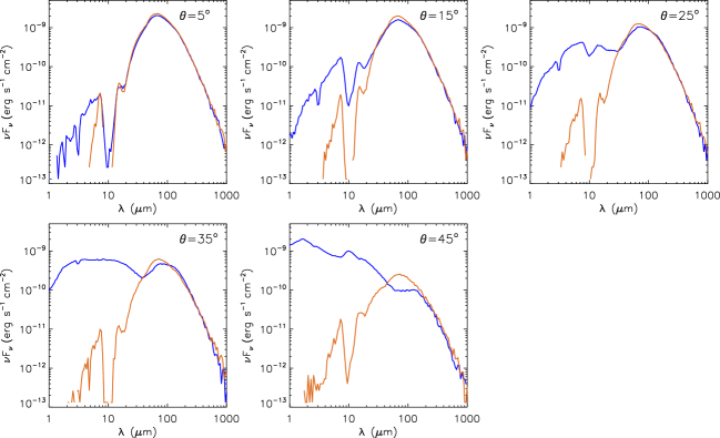
Figure 10.— Model 4 from section IV, calculated with the same parameters except for the cavity: in the five different panels, the same model is shown with five different cavity opening angles (see label inside each panel), and in each panel for two different cavity shapes (blue: polynomial-shaped cavity with exponent 1.5; orange: streamline-shaped cavity). Note that Model 4 has an inclination angle of 49°, and the best fit to HOPS 108 has $\theta$=5°.

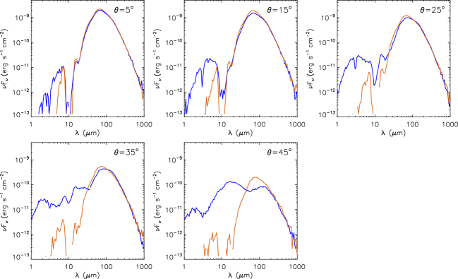
Figure 11.— Same as in Figure 10, but the models are shown for an inclination angle of 70°.

References

- Acke et al. (2010) Acke, B., Bouwman, J., Juhász, A., et al. 2010, ApJ, 718, 558
- Adams et al. (2012) Adams, J. D., Herter, T. L., Osorio, M., et al. 2012, ApJ, 749, L24
- Ali & DePoy (1995) Ali, B., & DePoy, D. L. 1995, AJ, 109, 709
- André et al. (1993) André, P., Ward-Thompson, D., & Barsony, M. 1993, ApJ, 406, 122
- André et al. (2010) André, P., Men’shchikov, A., Bontemps, S., et al. 2010, A&A, 518, L102
- Anglada (1995) Anglada, G., Rev. Mex. AA Ser. Conf., 1, 67
- Anglada (1996) Anglada, G., in ASP Conf. Ser. 93, Radio Emission from the Stars and the Sun, eds. A. R. Taylor & J. M. Paredes (San Francisco, CA: ASP), 3
- Anglada et al. (1998) Anglada, G., Villuendas, E., Estalella, R., et al. 1998, AJ, 116, 2953
- Bontemps et al. (1996) Bontemps, S., Andr’e, P., Terebey, S., & Cabrit, S. 1996, A&A, 311, 858
- Carpenter (2000) Carpenter, J. M. 2000, AJ, 120, 3139
- Chen et al. (1995) Chen, H., Myers, P. C., Ladd, E. F., & Wood, D. O. S. 1995, ApJ, 445, 377
- Chini et al. (1997) Chini, R., Reipurth, B., Ward-Thompson, D., et al. 1997, ApJ, 474, L135
- Crimier et al. (2009) Crimier, N., Ceccarelli, C., Lefloch, B., & Faure, A. 2009, A&A, 506, 1229
- D’Alessio et al. (1999) D’Alessio, P., Calvet, N., Hartmann, L., et al. 1999, ApJ, 527, 893
- D’Alessio et al. (2006) D’Alessio, P., Calvet, N., Hartmann, L., et al. 2006, ApJ, 638, 314
- Diolaiti et al. (2000) Diolaiti, E., Bendinelli, O., Bonaccini, D., et al. 2000, A&AS, 147, 335
- Fazio et al. (2004) Fazio, G. G., Hora, J. L., Allen, L. E., et al. 2004, ApJS,154, 10
- Fischer et al. (2010) Fischer, W. J., Megeath, S. T., Ali, B., et al. 2010, A&A, 518, L122
- Fischer et al. (2012) Fischer, W. J., Megeath, S. T., Tobin, J. J., et al. 2012, ApJ, 756, 99
- Furlan et al. (2008) Furlan, E., McClure, M., Calvet, N., et al. 2008, ApJS, 176, 184
- Gatley et al. (1974) Gatley, I., Becklin, E. E., Matthews, K., et al. 1974, ApJ, 191, L121
- Hartmann et al. (1996) Hartmann, L., Calvet, N., & Boss, A. 1996, ApJ, 464, 387
- Herter et al. (2012) Herter, T. L., Adams, J. D., De Buizer, J. M., et al. 2012, ApJ, 749, L18
- Hirota et al. (2007) Hirota, T., Bushimata, T., Choi, Y. K., et al. 2007, PASJ, 59, 897
- Houck et al. (2004) Houck, J. R., Roellig, T. L., van Cleve, J., et al. 2004, ApJS, 154, 18
- Johnson et al. (1990) Johnson, J. J., Gehrz, R. D., Jones, T. J., et al. 1990, AJ, 100, 518
- Johnstone & Bally (1999) Johnstone, D., & Bally, J, 1999, ApJ, 510, L49
- Johnstone et al. (2003) Johnstone, D., Boonman, A. M. S., & van Dishoeck, E. F. 2003, A&A, 412, 157
- Jones et al. (1994) Jones, T. J., Mergen, J., Odewahn, S., et al. 1994, AJ, 107, 2120
- Kama et al. (2010) Kama, M., Dominik, C., Maret, S., et al. 2010, A&A, 521, L39
- Kama et al. (2013) Kama, M., López-Sepulcre, A., Dominik, C., et al. 2013, A&A, 556, A57
- Kenyon, Calvet, & Hartmann (1993) Kenyon, S. J., Calvet, N., & Hartmann, L. 1993, ApJ, 414, 676
- Li et al. (2013) Li D., Kauffmann, J., Zhang, Q., & Chen, W. 2013, ApJ, 768, L5
- Lis et al. (1998) Lis, D. C., Serabyn, E., Keene, J. 1998, ApJ, 509, 299
- López-Sepulcre et al. (2013) López-Sepulcre, A., Taquet, V., Sánchez-Monge, Á., et al. 2013, A&A, 556, A62
- Manoj et al. (2013) Manoj, P., Watson, D. M., Neufeld, D. A., et al. 2013, ApJ, 763, 83
- Mathis (1990) Mathis, J. S. 1990, ARA&A, 28, 37
- McClure (2009) McClure, M. 2009, ApJ, 693, L81
- Megeath et al. (2012) Megeath, S. T., Gutermuth, R., Muzerolle, J., et al. 2012, AJ, 144, 192
- Menten et al. (2007) Menten, K. M., Reid, M. J., Forbrich, J., & Brunthaler, A. 2007, A&A, 474, 515
- Mezger et al. (1990) Mezger, P. G., Wink, J. E., & Zylka, R. 1990, A&A, 228, 95
- Nielbock et al. (2003) Nielbock, M., Chini, R., & Müller, S. A. H. 2003, A&A, 408, 245
- Ormel et al. (2011) Ormel, C. W., Min, M., Tielens, A. G. G. M., et al. 2011, A&A, 532, A43
- Peterson & Megeath (2008) Peterson, D. E., & Megeath, S. T. 2008, in Handbook of Star Forming Regions, Vol. 1, ed. B. Reipurth (Provo, UT: ASP Monograph Publications), 590
- Pilbratt et al. (2010) Pilbratt, G. L., Riedinger, J. R., Passvogel, T., et al. 2010, A&A, 518, L1
- Poglitsch et al. (2010) Poglitsch, A., Waelkens, C., Geis, N., et al. 2010, A&A, 518, L2
- Rayner et al. (1989) Rayner, J., McLean, I., McCaughrean, M., & Aspin, C. 1989, MNRAS, 241, 469
- Reipurth et al. (1999) Reipurth, B., Rodríguez, L. F., & Chini, R. 1999, AJ, 118, 983
- Rieke et al. (2004) Rieke, G. H., Young, E. T., Engelbracht, C. W., et al. 2004, ApJS, 154, 25
- Robitaille et al. (2006) Robitaille, T. P., Whitney, B. A., Indebetouw, R., et al. 2006, ApJS, 167, 256
- Shimajiri et al. (2008) Shimajiri, Y., Takahashi, S., Takakuwa, S., et al. 2008, ApJ, 683, 255
- Siringo et al. (2010) Siringo, G., Kreysa, E., De Breuck, C., et al. 2010, The Messenger, 139, 20
- Siringo et al. (2009) Siringo, G., Kreysa, E., Kovács, A., et al. 2009, A&A, 497, 945
- Smith & Rosen (2005) Smith, M. D., & Rosen, A. 2005, MNRAS, 357, 1370
- Stanke et al. (2010) Stanke, Th., Stutz, A. M., Tobin, J. J., et al. 2010, A&A, 518, L94
- Stutz et al. (2010) Stutz, A. M., Launhardt, R., Linz, H., et al. 2010, A&A, 518, L87
- Stutz et al. (2013) Stutz, A. M., Tobin, J. J., Stanke, Th., et al. 2013, ApJ, 767, 36
- Terebey, Shu, & Cassen (1984) Terebey, S., Shu, F. H., & Cassen, P. 1984, ApJ, 286, 529
- Tsujimoto et al. (2003) Tsujimoto, M., Koyama, K., Kobayashi, N., et al. 2003, AJ, 125, 1537
- Werner et al. (2004) Werner, M. W., Roellig, T. L., Low, F. J., et al. 2004, ApJS, 154, 1
- Whitney et al. (2003a) Whitney, B. A., Wood, K., Bjorkman, J. E., & Wolff, M. J. 2003, ApJ, 591, 1049
- Whitney et al. (2003b) Whitney, B. A., Wood, K., Bjorkman, J. E., & Cohen, M. 2003, ApJ, 598, 1079
- Young et al. (2012) Young, E. T., Becklin, E. E., Marcum, P. M., et al. 2012, ApJ, 749, L17