Resummation of the transverse-energy distribution in Higgs boson production at the Large Hadron Collider

Abstract:

We compute the resummed hadronic transverse-energy ($E_{T}$) distribution due to initial-state QCD radiation in the production of a Standard Model Higgs boson of mass 126 GeV by gluon fusion at the Large Hadron Collider, with matching to next-to-leading order calculations at large $E_{T}$. Effects of hadronization, underlying event and limited detector acceptance are estimated using aMC@NLO with the Herwig++ and Pythia8 event generators.

1 Introduction

The new particle discovered recently by the ATLAS [1] and CMS [2] Collaborations at the LHC looks very much like the Higgs boson of the Standard Model, although its properties remain to be fully explored. For this exploration, detailed predictions of the expected characteristics of Higgs production within the Standard Model will be essential, in order to optimize signal to background ratios and to search for any signs of new physics. One such characteristic is the amount and distribution of initial-state QCD radiation, which is predicted to be exceptionally high in production by gluon fusion and exceptionally low in vector boson fusion. A thorough understanding of initial-state radiation is therefore essential for the separation of these production mechanisms.

In the present paper we study the distribution of the total amount of transverse energy ($E_{T}$) emitted in Standard Model Higgs boson production by gluon fusion at the LHC. Results are presented at next-to-leading order (NLO) in QCD perturbation theory and also resummed to all orders in the QCD coupling $\alpha_{\mathrm{S}}$. The resummation applies to leading, next-to-leading and some important next-to-next-to-leading logarithms of $E_{T}/Q$ ((N)NLL) where $Q$ is the hard process scale, taken to be the Higgs mass $m_{H}$. Thus it improves the treatment of the small-$E_{T}$ region, where the fixed-order prediction diverges whereas the actual distribution must tend to zero as $E_{T}\to 0$. By matching the resummed prediction to the NLO result valid at large $E_{T}$, we provide a uniform description from the low-$E_{T}$ to the high-$E_{T}$ region.

Our approach follows on from Ref. [3], based in turn on the early work on $E_{T}$ resummation in vector-boson production [4, 5, 6] and closely related to the resummation of transverse momentum in vector-boson [7, 8, 9, 10] and Higgs production [11, 12, 13, 14]. We make a number of improvements relative to Ref. [3], including:

• Predictions for the experimentally relevant Higgs mass of 126 GeV, at centre-of-mass energies $\sqrt{s}=8$ and $14$ TeV;

• Fixed-order predictions to NLO, i.e. ${\cal O}(\alpha_{\mathrm{S}}^{4})$.

• Expansion of the $E_{T}$ resummation formula to NLO, and demonstration that to this order the structure of the logarithmic terms is consistent with the fixed-order prediction;

• Matching of the resummed and NLO predictions across the whole range of $E_{T}$;

• A constraint on the perturbative unitarity of the prediction, using the method of Ref. [11], which reduces the impact of logarithmic terms in the large-$E_{T}$ region;

• Studies of the effects of renormalization scale variation and unknown higher-order terms;

• Monte Carlo studies of the effects of hadron-level cuts on pseudorapidity and transverse momentum, with fixed-order matching to parton showers using aMC@NLO interfaced to Herwig++ and Pythia8.

The paper is organized as follows. In Sec. 2, we review the resummation procedure and then describe the necessary modifications to implement the unitarity condition mentioned above. This involves some changes in the formalism and the evaluation of new integrals in this prescription. In Sec. 3, we expand our resummed result to next-to-leading order in order to match our results to the fixed-order prediction at this accuracy. This renders our predictions positive throughout the $E_{T}$-range. In Sec. 4, we investigate the $E_{T}$ distribution further through Monte Carlo studies. We first reweight Monte Carlo results to our analytic distribution and then investigate the impact of hadronisation and underlying event. We end the main text in Sec. 5 with conclusions and discussion. A number of appendices then contain supplementary results.

2 Resummation of logarithmically enhanced terms

Here we summarize the results of Ref. [3] as applied to Higgs boson production. The resummed component of the transverse-energy distribution in the process $h_{1}h_{2}\to HX$ at scale $Q$ has the form

$$\left[\frac{d\sigma_{H}}{dQ^{2}\;dE_{T}}\right]_{{\rm res.}} = \frac{1}{2\pi}\sum_{a,b}\int_{0}^{1}dx_{1}\int_{0}^{1}dx_{2}\int_{-\infty}^{+\infty}d\tau\;{\rm e}^{-i\tau E_{T}}\;f_{a/h_{1}}(x_{1},\mu)\;f_{b/h_{2}}(x_{2},\mu)$$ (1)

$$\cdot W_{ab}^{H}(x_{1}x_{2}s;Q,\tau,\mu)$$

where $f_{a/h}(x,\mu)$ is the parton distribution function (PDF) of parton $a$ in hadron $h$ at factorization scale $\mu$, taken to be the same as the renormalization scale here (we illustrate the impact of varying this scale in Sec. 3). In what follows we use the ${\overline{\rm MS}}$ renormalization scheme. To take into account the constraint that the transverse energies of the emitted partons should sum to $E_{T}$, the resummation procedure is carried out in the domain that is Fourier conjugate to $E_{T}$. The transverse-energy distribution (1) is thus obtained by performing the inverse Fourier transformation with respect to the “transverse time”, $\tau$. The factor $W_{ab}^{H}$ is the perturbative and process-dependent partonic cross section that embodies the all-order resummation of the large logarithms $\ln(Q\tau)$. Since $\tau$ is conjugate to $E_{T}$, the limit $E_{T}\ll Q$ corresponds to $Q\tau\gg 1$.

As in the case of transverse-momentum resummation [20], the resummed partonic cross section can be written in the following form:

$$W_{ab}^{H}(s;Q,\tau,\mu) = \int_{0}^{1}dz_{1}\int_{0}^{1}dz_{2}\;C_{ga}(\alpha_{\mathrm{S}}(\mu),z_{1};\tau,\mu)\;C_{gb}(\alpha_{\mathrm{S}}(\mu),z_{2};\tau,\mu)\;\delta(Q^{2}-z_{1}z_{2}s)$$ (2)

$$\cdot \sigma_{gg}^{H}(Q,\alpha_{\mathrm{S}}(Q))\;S_{g}(Q,\tau)\;\;.$$

Here $\sigma_{gg}^{H}$ is the cross section for the partonic subprocess of gluon fusion, $gg\to H$, through a massive-quark loop:

$$\sigma_{gg}^{H}(Q,\alpha_{\mathrm{S}}(Q))=\delta(Q^{2}-m_{H}^{2})\sigma_{0}^{H}\;,$$ (3)

where in the limit of infinite quark mass

$$\sigma_{0}^{H}=\frac{\alpha_{\mathrm{S}}^{2}(m_{H})G_{F}m_{H}^{2}}{288\pi\sqrt{2}}\;.$$ (4)

$S_{g}(Q,\tau)$ is the appropriate gluon form factor, which in the case of $E_{T}$ resummation takes the form [5, 6]

$$S_{g}(Q,\tau)=\exp\left\{-2\int_{0}^{Q}\frac{dq}{q}\left[2A_{g}(\alpha_{\mathrm{S}}(q))\;\ln\frac{Q}{q}+B_{g}(\alpha_{\mathrm{S}}(q))\right]\left(1-{\rm e}^{iq\tau}\right)\right\}\;.$$ (5)

The functions $A_{g}(\alpha_{\mathrm{S}}),B_{g}(\alpha_{\mathrm{S}})$, as well as the coefficient functions $C_{ga}$ in Eq. (2), contain no $\ln(Q\tau)$ terms and are perturbatively computable as power expansions with constant coefficients:

$$A_{g}(\alpha_{\mathrm{S}}) = \sum_{n=1}^{\infty}\left(\frac{\alpha_{\mathrm{S}}}{\pi}\right)^{n}A_{g}^{(n)}\;\;,$$ (6)

$$B_{g}(\alpha_{\mathrm{S}}) = \sum_{n=1}^{\infty}\left(\frac{\alpha_{\mathrm{S}}}{\pi}\right)^{n}B_{g}^{(n)}\;\;,$$ (7)

$$C_{ga}(\alpha_{\mathrm{S}},z) = \delta_{ga}\,\delta(1-z)+\sum_{n=1}^{\infty}\left(\frac{\alpha_{\mathrm{S}}}{\pi}\right)^{n}C_{ga}^{(n)}(z)\;\;.$$ (8)

Thus a calculation to NLO in $\alpha_{\mathrm{S}}$ involves the coefficients $A_{g}^{(1)}$, $A_{g}^{(2)}$, $B_{g}^{(1)}$, $B_{g}^{(2)}$ and $C_{ga}^{(1)}$. The coefficients $A_{g}^{(1)}$, $A_{g}^{(2)}$, $B_{g}^{(1)}$ and $C_{ga}^{(1)}$ read [21, 22]

$$A_{g}^{(1)}=C_{A}\;,\quad A_{g}^{(2)}=\frac{1}{6}C_{A}\left[C_{A}\left(\frac{67}{6}-\frac{\pi^{2}}{2}\right)-\frac{5}{3}n_{f}\right]\;,\quad B_{g}^{(1)}=-\frac{1}{6}(11C_{A}-2n_{f})\;,$$

$$C_{gg}^{(1)}(z)=\frac{1}{4}\left[C_{A}\left(2-\frac{\pi^{2}}{3}\right)+5+4\pi^{2}\right]\delta(1-z)\equiv c^{(1)}_{g}\delta(1-z)\;,$$

$$C_{gq}^{(1)}(z)=C_{g\bar{q}}^{(1)}(z)=\frac{1}{2}C_{F}z\,.$$ (9)

The coefficient $B_{g}^{(2)}$ for the Higgs transverse-momentum spectrum is [23, 24]

$$\overline{B}_{g}^{(2)}=C_{A}^{2}\left(\frac{23}{24}+\frac{11}{18}\pi^{2}-\frac{3}{2}\zeta_{3}\right)+\frac{1}{2}C_{F}\,n_{f}-C_{A}\,n_{f}\left(\frac{1}{12}+\frac{\pi^{2}}{9}\right)-\frac{11}{8}C_{F}C_{A}\,.$$ (10)

However, the value of the coefficient $B_{g}^{(2)}$ for the transverse energy in Higgs production could be different. In Sec. 3, we will perform a fit to the fixed-order NLO result at small transverse energy, with this coefficient as a free parameter.

Returning to Eq. (1), we may recast it in a form with a real integrand as

$$\left[\frac{d\sigma_{H}}{dQ^{2}\;dE_{T}}\right]_{{\rm res.}} = \frac{1}{\pi s}\int_{0}^{\infty}d\tau\;{\rm e}^{-F_{g}^{(R)}(Q,\tau)}\Bigl{[}R_{g}^{(R)}(s;Q,\tau)\cos\{F_{g}^{(I)}(Q,\tau)+\tau E_{T}\}$$ (11)

$$+R_{g}^{(I)}(s;Q,\tau)\sin\{F_{g}^{(I)}(Q,\tau)+\tau E_{T}\}\Bigr{]}\,\sigma_{gg}^{H}(Q,\alpha_{\mathrm{S}}(Q))$$

where $F_{g}^{(R)}$ and $F_{g}^{(I)}$ are the real and imaginary parts of

$$F_{g}(Q,\tau)=2\int_{0}^{Q}\frac{dq}{q}\left[2A_{g}(\alpha_{\mathrm{S}}(q))\;\ln\frac{Q}{q}+B_{g}(\alpha_{\mathrm{S}}(q))\right]\left(1-{\rm e}^{iq\tau}\right)\,.$$ (12)

As explained in [3], the coefficient functions in Eq. (2) contain logarithms of $\mu\tau$, which are eliminated by the choice of factorization scale $\mu_{F}=\tau_{0}/\tau$, where $\tau_{0}=\exp(-\gamma_{\rm E})=0.56146\ldots$, $\gamma_{\rm E}$ being the Euler-Mascheroni constant. The resulting expressions for $R_{g}^{(R,I)}$ are

$$R_{g}^{(R)}(\xi,\tau) =\int_{\xi}^{1}\frac{dx_{1}}{x_{1}}\Biggl{\{}f_{g/h_{1}}(x_{1})f_{g/h_{2}}\left(\frac{\xi}{x_{1}}\right)\left(1+\frac{\alpha_{\mathrm{S}}}{\pi}2c^{(1)}_{g}\right)$$ (13)

$$+\frac{\alpha_{\mathrm{S}}}{\pi}\int_{\xi/x_{1}}^{1}\frac{dz}{z}\left[f_{g/h_{1}}(x_{1})f_{s/h_{2}}\left(\frac{\xi}{zx_{1}}\right)+f_{s/h_{1}}(x_{1})f_{g/h_{2}}\left(\frac{\xi}{zx_{1}}\right)\right]\frac{1}{2}C_{F}z\Biggr{\}}\;,$$

$$R_{g}^{(I)}(\xi,\tau) =\frac{\alpha_{\mathrm{S}}}{2}\int_{\xi}^{1}\frac{dx_{1}}{x_{1}}\int_{0}^{1}\frac{dz}{z}\Biggl{\{}2f_{g/h_{1}}(x_{1})f_{g/h_{2}}\left(\frac{\xi}{zx_{1}}\right)P_{gg}(z)$$

$$+\left[f_{g/h_{1}}(x_{1})f_{s/h_{2}}\left(\frac{\xi}{zx_{1}}\right)+f_{s/h_{1}}(x_{1})f_{g/h_{2}}\left(\frac{\xi}{zx_{1}}\right)\right]P_{gq}(z)\Biggr{\}}$$

$$= \frac{\alpha_{\mathrm{S}}}{2}\int_{\xi}^{1}\frac{dx_{1}}{x_{1}}\Biggl{\{}2f_{g/h_{1}}(x_{1})f_{g/h_{2}}\left(\frac{\xi}{x_{1}}\right)\left[2C_{A}\ln\left(1-\frac{\xi}{x_{1}}\right)+\frac{1}{6}(11C_{A}-2n_{f})\right]$$

$$+\int_{\xi/x_{1}}^{1}\frac{dz}{z}\Biggl{[}4C_{A}f_{g/h_{1}}(x_{1})\left\{f_{g/h_{2}}\left(\frac{\xi}{zx_{1}}\right)\left[\frac{z}{1-z}+\frac{1-z}{z}+z(1-z)\right]-f_{g/h_{2}}\left(\frac{\xi}{x_{1}}\right)\frac{z}{1-z}\right\}$$

$$+\left\{f_{g/h_{1}}(x_{1})f_{s/h_{2}}\left(\frac{\xi}{zx_{1}}\right)+f_{s/h_{1}}(x_{1})f_{g/h_{2}}\left(\frac{\xi}{zx_{1}}\right)\right\}C_{F}\frac{1+(1-z)^{2}}{z}\Biggr{]}\Biggr{\}},$$

where $f_{s}=\sum_{q}(f_{q}+f_{\bar{q}})$ and all PDFs and coefficient functions are understood to be evaluated at scale $\mu_{F}=\tau_{0}/\tau$. We have defined $\xi=Q^{2}/s$ for convenience.

2.1 Evaluation of the exponent

We now seek to evaluate the exponent of the form factor, (12), analytically. We will use the method of Ref. [11] where the analogous calculation was performed for transverse-momentum resummation. In the notation of that paper, we have, for a renormalization scale $\mu_{R}$,

$$G_{g}(a_{R},L)\equiv-2\int_{b_{0}/b}^{Q}\frac{dq}{q}\left[2A_{g}(\alpha_{\mathrm{S}}(q))\;\ln\frac{Q}{q}+B_{g}(\alpha_{\mathrm{S}}(q))\right]=L\,g_{1}(Y)+g_{2}(Y)+a_{R}\,g_{3}(Y)+\ldots$$ (14)

where $a_{R}=\alpha_{\mathrm{S}}(\mu_{R})/\pi$, $L=2\ln(Qb/b_{0})$, $Y=\beta_{0}a_{R}L$ and $\beta_{0}=(11C_{A}-2n_{f})/12$ is the lowest-order coefficients of the beta function:

$$\frac{d\ln a_{R}}{d\ln\mu_{R}^{2}}=\beta(a_{R})=-\sum_{n=0}^{\infty}\beta_{n}a_{R}^{n+1}.$$ (15)

The term $Lg_{1}(Y)$ collects the LL contributions $\alpha_{\mathrm{S}}^{n}L^{n+1}$, the function $g_{2}$ resums the NLL contributions $\alpha_{\mathrm{S}}^{n}L^{n}$, the function $g_{3}$ controls the NNLL terms $\alpha_{\mathrm{S}}^{n}L^{n-1}$, and so forth. We will give the explicit form of the $g_{i}$ functions below. We can therefore deduce that in general

$$-2\int_{Q_{0}}^{Q}\frac{dq}{q}\left[2A_{g}(\alpha_{\mathrm{S}}(q))\;\ln\frac{Q}{q}+B_{g}(\alpha_{\mathrm{S}}(q))\right]=2\lambda g_{1}(y)+g_{2}(y)+a_{R}\,g_{3}(y)+\ldots$$ (16)

where now

$$y\equiv 2\beta_{0}a_{R}\lambda\qquad{\rm and}\qquad\lambda\equiv\ln(Q/Q_{0})\;.$$ (17)

Now by expressing $\alpha_{\mathrm{S}}(q)$ in terms of $\alpha_{\mathrm{S}}(Q)$ and relating this in turn to $\alpha_{\mathrm{S}}(\mu_{R})$, we can write the integrand in (16) as a function of $\ln(Q/q)$, and then use the result

$$\int_{Q_{0}}^{Q}\frac{dq}{q}f\left(\ln\frac{Q}{q}\right)=f\left(\frac{d}{du}\right)\frac{1}{u}\left.\left({\rm e}^{\lambda u}-1\right)\right|_{u=0}\,,$$ (18)

which is easily seen by expanding the exponential. This allows one to calculate the $g_{i}$ functions explicitly. They are given by [25, 26, 11]:

$$g_{1}(y) = \frac{A_{g}^{(1)}}{\beta_{0}y}\left(y+\ln(1-y)\right)\,,$$

$$g_{2}(y) = \frac{B_{g}^{(1)}}{\beta_{0}}\ln(1-y)-\frac{A_{g}^{(2)}}{\beta_{0}^{2}}\left(\frac{y}{1-y}+\ln(1-y)\right)$$

$$\ +\frac{A_{g}^{(1)}\beta_{1}}{\beta_{0}^{3}}\left(\frac{1}{2}\ln^{2}(1-y)+\frac{y+\ln(1-y)}{1-y}\right)+\frac{A_{g}^{(1)}}{\beta_{0}}\left(\frac{y}{1-y}+\ln(1-y)\right)\ln\left(\frac{Q^{2}}{\mu_{R}^{2}}\right)\,,$$

$$g_{3}(y) = -\frac{A_{g}^{(3)}}{2\beta_{0}^{2}}\left(\frac{y}{1-y}\right)^{2}-\frac{B_{g}^{(2)}}{\beta_{0}}\frac{y}{1-y}+\frac{A_{g}^{(2)}\beta_{1}}{\beta_{0}^{3}}\frac{y(3y-2)-2(1-2y)\ln(1-y)}{2(1-y)^{2}}$$

$$\ +\frac{A_{g}^{(1)}}{\beta_{0}^{4}}\left(\frac{\beta_{1}^{2}(1-2y)\ln^{2}(1-y)}{2(1-y)^{2}}+\ln(1-y)\left(\beta_{0}\beta_{2}-\beta_{1}^{2}+\frac{\beta_{1}^{2}}{1-y}\right)\right.$$

$$\qquad\left.+\frac{y(\beta_{0}\beta_{2}(2-3y)+\beta_{1}^{2}y)}{2(1-y)^{2}}\right)+\frac{B_{g}^{(1)}\beta_{1}}{\beta_{0}^{2}}\frac{y+\ln(1-y)}{1-y}-\frac{A_{g}^{(1)}}{2}\frac{y^{2}}{(1-y)^{2}}\ln^{2}\left(\frac{Q^{2}}{\mu_{R}^{2}}\right)$$

$$\ +\left(B_{g}^{(1)}\frac{y}{1-y}+\frac{A_{g}^{(2)}}{\beta_{0}}\frac{y^{2}}{(1-y)^{2}}+A_{g}^{(1)}\frac{\beta_{1}}{\beta_{0}^{2}}\left(\frac{y}{1-y}+\frac{(1-2y)\ln(1-y)}{(1-y)^{2}}\right)\right)\ln\left(\frac{Q^{2}}{\mu_{R}^{2}}\right).$$

Now, the actual integral we require is

$$F_{g}(\alpha_{\mathrm{S}},\lambda)\equiv 2\int_{0}^{Q}\frac{dq}{q}\left[2A_{g}(\alpha_{\mathrm{S}}(q))\;\ln\frac{Q}{q}+B_{g}(\alpha_{\mathrm{S}}(q))\right]\left(1-{\rm e}^{iq\tau}\right)$$ (20)

and so we must introduce $\left(1-{\rm e}^{iq\tau}\right)$ in the integrand. The analogue of Eq. (18) is

$$\int_{0}^{Q}\frac{dq}{q}f\left(\ln\frac{Q}{q}\right)\left(1-{\rm e}^{iq\tau}\right)=f\left(\frac{d}{du}\right)\left.{\cal J}(Q\tau;-u)\right|_{u=0}$$ (21)

where the generating function

$${\cal J}(Q\tau;u) = \int_{0}^{Q}\frac{dq}{q}\left(\frac{q}{Q}\right)^{u}\left(1-{\rm e}^{iq\tau}\right)$$ (22)

$$= \frac{1}{u}-\left(-iQ\tau\right)^{-u}\gamma(u,-iQ\tau)\,,$$

$\gamma(u,z)$ being the incomplete gamma function,

$$\gamma(u,z)=\Gamma(u)-z^{u-1}{\rm e}^{-z}\sum_{k=0}^{\infty}\frac{\Gamma(u)}{\Gamma(u-k)}z^{-k}\;.$$ (23)

The series represents power corrections, which we do not wish to include in the resummation, so we write instead

$${\cal J}(Q\tau;-u) = \frac{1}{u}\left[\left(-iQ\tau\right)^{u}\Gamma(1-u)-1\right]$$ (24)

$$= \frac{1}{u}\left[\exp\left(\lambda u+\sum_{k=2}\frac{\zeta_{k}}{k}u^{k}\right)-1\right]\equiv\frac{1}{u}\left[{\rm e}^{\lambda u}Z(u)-1\right]$$

where now

$$\lambda=\ln\left(\frac{Q\tau}{i\tau_{0}}\right)\,,$$ (25)

i.e. we have chosen $Q_{0}=i{\rm e}^{-\gamma_{\rm E}}/\tau=i\tau_{0}/\tau$ in (17), and

$$Z(u)\equiv\exp\left(\sum_{k=2}\frac{\zeta_{k}}{k}u^{k}\right)=\tau_{0}^{u}\Gamma(1-u)\,.$$ (26)

Now

$$\frac{1}{u}\left[{\rm e}^{\lambda u}Z(u)-1\right]=\frac{Z(u)}{u}\left[{\rm e}^{\lambda u}-1\right]+\frac{1}{u}\left[Z(u)-1\right]$$ (27)

and the second term involves no logarithms, so again we drop it from the resummation. We show in Appendix A that the first term implies that

$$F_{g}(\alpha_{\mathrm{S}},\lambda)\equiv 2\int_{0}^{Q}\frac{dq}{q}\left[2A_{g}(\alpha_{\mathrm{S}}(q))\;\ln\frac{Q}{q}+B_{g}(\alpha_{\mathrm{S}}(q))\right]\left(1-{\rm e}^{iq\tau}\right)=-Z\left(\frac{d}{d\lambda}\right)G_{g}(\alpha_{\mathrm{S}},2\lambda)\,,$$ (28)

where $G_{g}$ was defined in Eq. (14). Now

$$Z\left(\frac{d}{d\lambda}\right)=1+\frac{\zeta_{2}}{2}\frac{d^{2}}{d\lambda^{2}}+\frac{\zeta_{3}}{3}\frac{d^{3}}{d\lambda^{3}}+\ldots$$ (29)

where $\zeta_{2}=\pi^{2}/6$, so

$$F_{g}(\alpha_{\mathrm{S}},\lambda)=-2\lambda g_{1}(y)-g_{2}(y)-a_{R}\widetilde{g}_{3}(y)+\ldots$$ (30)

where

$$\widetilde{g}_{3}(y) = g_{3}(y)+\frac{\pi^{2}}{12a_{R}}\frac{d^{2}}{d\lambda^{2}}[2\lambda g_{1}(y)]$$ (31)

$$= g_{3}(y)-\frac{\pi^{2}}{3}\frac{A_{g}^{(1)}}{(1-y)^{2}}\,.$$

The other terms from (29) contribute logarithms only at the level of $g_{4}$ and beyond, so we do not consider them.

Following Ref. [11], we can now enforce the ‘unitarity’ condition, $F_{g}\to 0$ as $\tau\to 0$, by a shift of argument of the logarithm:

$$\lambda\to\widetilde{\lambda}=\ln\left(1+\frac{Q\tau}{i\tau_{0}}\right)=\frac{1}{2}\ln\left(1+\frac{Q^{2}\tau^{2}}{\tau_{0}^{2}}\right)-i\arctan\left(\frac{Q\tau}{\tau_{0}}\right)\,,$$ (32)

so that now $y=2\beta_{0}\alpha_{\mathrm{S}}(\mu_{R}^{2})\widetilde{\lambda}/\pi$. We must apply a corresponding shift in the factorization scale of the parton distributions and coefficient functions (given explicitly below in Eqs. (3.1)). They are now evaluated at a scale of

$$\widetilde{\mu}_{F}=\frac{Q}{\sqrt{1+Q^{2}\tau^{2}/\tau_{0}^{2}}}$$ (33)

instead of $\mu_{F}=\tau_{0}/\tau$, and one must also replace $\alpha_{\mathrm{S}}(\mu_{F})/2$ in the coefficient of $R_{g}^{(I)}$ by

$$\frac{\alpha_{\mathrm{S}}(\widetilde{\mu}_{F})}{\pi}\arctan\left(\frac{Q\tau}{\tau_{0}}\right)\,.$$ (34)

We show in Appendix B that the vanishing of the transverse-energy distribution for $E_{T}<0$ implies a dispersion relation between the real and imaginary parts of its Fourier transform. This allows (11) to be written in the simpler equivalent form

$$\left[\frac{d\sigma_{H}}{dQ^{2}\;dE_{T}}\right]_{{\rm res.}} = \frac{2}{\pi s}\int_{0}^{\infty}d\tau\;{\rm e}^{-F_{g}^{(R)}(Q,\tau)}\cos(\tau E_{T})\Bigl{[}R_{g}^{(R)}(s;Q,\tau)\cos\{F_{g}^{(I)}(Q,\tau)\}$$ (35)

$$-R_{g}^{(I)}(s;Q,\tau)\sin\{F_{g}^{(I)}(Q,\tau)\}\Bigr{]}\,\sigma_{gg}^{H}(Q,\alpha_{\mathrm{S}}(Q))$$

and implies that

$$\int_{0}^{\infty}dE_{T}\,\left[\frac{d\sigma_{H}}{dQ^{2}\;dE_{T}}\right]_{{\rm res.}}=\frac{1}{s}R_{g}^{(R)}(s;Q,0)\,\sigma_{gg}^{H}(Q,\alpha_{\mathrm{S}}(Q))\,,$$ (36)

where, on account of (33), the parton distributions in $R_{g}^{(R)}(s;Q,0)$ are evaluated at scale $Q$.

3 Matching to fixed order

We now match the resummed expression derived above to the NLO perturbative expansion of the transverse energy distribution, taking care to avoid double counting of the terms already contained in the resummation.

3.1 Expansion of the resummed prediction

Performing the expansion of Eq. (30) in powers of $a_{R}\equiv\alpha_{\mathrm{S}}(\mu_{R}^{2})/\pi$, we find

$$-2\lambda g_{1} = 2A_{g}^{(1)}\lambda^{2}a_{R}+\frac{8}{3}\beta_{0}A_{g}^{(1)}\lambda^{3}a_{R}^{2}+{\cal O}(a_{R}^{3})$$

$$-g_{2} = 2B_{g}^{(1)}\lambda a_{R}+2\left[A_{g}^{(2)}+\beta_{0}B_{g}^{(1)}-\beta_{0}A_{g}^{(1)}\ln\left(\frac{Q^{2}}{\mu_{R}^{2}}\right)\right]\lambda^{2}a_{R}^{2}+{\cal O}(a_{R}^{3})$$

$$-a_{R}\widetilde{g}_{3} = \frac{\pi^{2}}{3}A_{g}^{(1)}a_{R}+2\left[B_{g}^{(2)}+\frac{2}{3}\pi^{2}\beta_{0}A_{g}^{(1)}-\beta_{0}B_{g}^{(1)}\ln\left(\frac{Q^{2}}{\mu_{R}^{2}}\right)\right]\lambda a_{R}^{2}+{\cal O}(a_{R}^{3})\,,$$ (37)

so that to NLO

$$F_{g}(\alpha_{\mathrm{S}},\lambda)=a_{R}F_{1}+a_{R}^{2}F_{2}$$ (38)

where, following the shift $\lambda\to\widetilde{\lambda}$ according to Eq. (32)

$$F_{1} = 2A_{g}^{(1)}\left(\widetilde{\lambda}^{2}+\frac{\pi^{2}}{6}\right)+2B_{g}^{(1)}\widetilde{\lambda}$$

$$F_{2} = \frac{8}{3}\beta_{0}A_{g}^{(1)}\widetilde{\lambda}^{3}+2\left[A_{g}^{(2)}+\beta_{0}B_{g}^{(1)}-\beta_{0}A_{g}^{(1)}\ln\left(\frac{Q^{2}}{\mu_{R}^{2}}\right)\right]\widetilde{\lambda}^{2}$$ (39)

$$+2\left[B_{g}^{(2)}+\frac{2}{3}\pi^{2}\beta_{0}A_{g}^{(1)}-\beta_{0}B_{g}^{(1)}\ln\left(\frac{Q^{2}}{\mu_{R}^{2}}\right)\right]\widetilde{\lambda}\,.$$

Similarly, evaluating all PDFs at scale $\mu=Q$, we can write to NLO

$$R_{g}(\tau)=R_{0}+a_{R}\left(R_{1}+\widetilde{\lambda}R^{\prime}_{1}\right)+a_{R}^{2}\left(R_{2}+\widetilde{\lambda}R^{\prime}_{2}+\widetilde{\lambda}^{2}R^{\prime\prime}_{2}\right)$$ (40)

so that

$$S_{g}R_{g} = R_{0}+a_{R}R_{1}+a_{R}^{2}R_{2}+a_{R}\left(\widetilde{\lambda}R^{\prime}_{1}-F_{1}R_{0}\right)$$ (41)

$$+ a_{R}^{2}\left[\widetilde{\lambda}R^{\prime}_{2}+\widetilde{\lambda}^{2}R^{\prime\prime}_{2}-(F_{2}-\frac{1}{2}F_{1}^{2})R_{0}-F_{1}(R_{1}+\widetilde{\lambda}R^{\prime}_{1})\right]$$

where

$$R_{0} = \int_{\xi}^{1}\frac{dx_{1}}{x_{1}}f_{g}(x_{1})f_{g}\left(\frac{\xi}{x_{1}}\right)$$

$$R_{1} = \int_{\xi}^{1}\frac{dx_{1}}{x_{1}}\Biggl{\{}2c^{(1)}_{g}f_{g}(x_{1})f_{g}\left(\frac{\xi}{x_{1}}\right)+C_{F}\int_{\xi/x_{1}}^{1}dz\,f_{s}(x_{1})f_{g}\left(\frac{\xi}{zx_{1}}\right)\Biggr{\}}$$

$$R^{\prime}_{1} = -\int_{\xi}^{1}\frac{dx_{1}}{x_{1}}\Biggl{\{}2f_{g}(x_{1})f_{g}\left(\frac{\xi}{x_{1}}\right)\left[2C_{A}\ln\left(1-\frac{\xi}{x_{1}}\right)+\frac{1}{6}(11C_{A}-2n_{f})\right]$$ (42)

$$+\int_{\xi/x_{1}}^{1}\frac{dz}{z}\Biggl{[}4C_{A}f_{g}(x_{1})\left\{f_{g}\left(\frac{\xi}{zx_{1}}\right)\left[\frac{z}{1-z}+\frac{1-z}{z}+z(1-z)\right]-f_{g}\left(\frac{\xi}{x_{1}}\right)\frac{z}{1-z}\right\}$$

$$+2C_{F}f_{s}(x_{1})f_{g}\left(\frac{\xi}{zx_{1}}\right)\frac{1+(1-z)^{2}}{z}\Biggr{]}\Biggr{\}}.$$

Performing the Fourier transformation (1), we find terms involving the integrals

$${\cal I}_{p}(E_{T},Q)=\frac{1}{2\pi}\int_{-\infty}^{+\infty}d\tau\;{\rm e}^{-i\tau E_{T}}\ln^{p}\left(1+\frac{Q\tau}{i\tau_{0}}\right)$$ (43)

with $p=1,2,3,4$, which may be evaluated from

$${\cal I}_{p}(E_{T},Q)=\frac{d^{p}}{du^{p}}{\cal I}(E_{T},Q;u)|_{u=0}$$ (44)

with generating function

$${\cal I}(E_{T},Q;u)=\frac{1}{2\pi}\int_{-\infty}^{+\infty}d\tau\;{\rm e}^{-i\tau E_{T}}\left(1+\frac{Q\tau}{i\tau_{0}}\right)^{u}\;.$$ (45)

Writing

$$1+\frac{Q\tau}{i\tau_{0}}=\frac{zQ}{\tau_{0}E_{T}}$$ (46)

we have

$${\cal I}(E_{T},Q;u)=-\frac{i}{2\pi E_{T}}\left(\frac{Q}{E_{T}\tau_{0}}\right)^{u}\int_{-i\infty}^{+i\infty}dz\;z^{u}\,{\rm e}^{z-\tau_{0}E_{T}/Q}\;.$$ (47)

We can safely deform the integration contour around the branch cut along the negative real axis to obtain

$${\cal I}(E_{T},Q;u) = -\frac{u}{E_{T}}\left(\frac{Q}{E_{T}}\right)^{u}\frac{\exp(u\gamma_{\rm E}-\tau_{0}E_{T}/Q)}{\Gamma(1-u)}$$ (48)

$$= -\frac{u}{E_{T}}\left(\frac{Q}{E_{T}}\right)^{u}\exp\left(-\frac{\tau_{0}E_{T}}{Q}-\sum_{k=2}^{\infty}\frac{\zeta_{k}}{k}u^{k}\right)\;.$$

This gives

$${\cal I}_{1}(E_{T},Q) = -\frac{1}{E_{T}}{\rm e}^{-\tau_{0}E_{T}/Q}$$

$${\cal I}_{2}(E_{T},Q) = -\frac{2}{E_{T}}\ln\left(\frac{Q}{E_{T}}\right){\rm e}^{-\tau_{0}E_{T}/Q}$$

$${\cal I}_{3}(E_{T},Q) = -\frac{3}{E_{T}}\left[\ln^{2}\left(\frac{Q}{E_{T}}\right)-\frac{\pi^{2}}{6}\right]{\rm e}^{-\tau_{0}E_{T}/Q}$$

$${\cal I}_{4}(E_{T},Q) = -\frac{4}{E_{T}}\left[\ln^{3}\left(\frac{Q}{E_{T}}\right)-\frac{\pi^{2}}{2}\ln\left(\frac{Q}{E_{T}}\right)-2\zeta_{3}\right]{\rm e}^{-\tau_{0}E_{T}/Q}\;.$$ (49)

Therefore the NLO expansion of the resummed expression is

$$\left[\frac{E_{T}}{\sigma_{0}^{H}}\frac{d\sigma_{H}}{dE_{T}}\right]_{\rm resum,NLO} = \Bigl{[}a_{R}(G_{0}R_{0}+G^{\prime}_{1}R^{\prime}_{1})+a_{R}^{2}(H_{0}R_{0}+H_{1}R_{1}$$ (50)

$$+H^{\prime}_{1}R^{\prime}_{1}+H^{\prime}_{2}R^{\prime}_{2}+H^{\prime\prime}_{2}R^{\prime\prime}_{2})\Bigr{]}{\rm e}^{-\tau_{0}E_{T}/Q}$$

where, writing $L=\ln(Q/E_{T})$,

$$G_{0} = H_{1}=4A_{g}^{(1)}L+2B_{g}^{(1)}\;,\;\;\;G^{\prime}_{1}=-1\;,$$

$$H_{0} = 4L\left[A_{g}^{(2)}+\beta_{0}B_{g}^{(1)}-\beta_{0}A_{g}^{(1)}\ln\left(\frac{Q^{2}}{\mu_{R}^{2}}\right)\right]+8\beta_{0}A_{g}^{(1)}\left(L^{2}-\frac{\pi^{2}}{6}\right)$$

$$+ 2\left[B_{g}^{(2)}+\frac{2}{3}\pi^{2}\beta_{0}A_{g}^{(1)}-\beta_{0}B_{g}^{(1)}\ln\left(\frac{Q^{2}}{\mu_{R}^{2}}\right)\right]-8(A_{g}^{(1)})^{2}\left(L^{3}-\frac{\pi^{2}}{3}L-2\zeta_{3}\right)$$

$$- 12A_{g}^{(1)}B_{g}^{(1)}\left(L^{2}-\frac{\pi^{2}}{9}\right)-4(B_{g}^{(1)})^{2}L\;,$$

$$H^{\prime}_{1} = 6A_{g}^{(1)}\left(L^{2}-\frac{\pi^{2}}{9}\right)+4B_{g}^{(1)}L\;,\;\;\;H^{\prime}_{2}=-1\;,\;\;\;H^{\prime\prime}_{2}=-2L\;.$$ (51)

We evaluate the coefficients $R_{0},R_{1},R^{\prime}_{1}$ explicitly from Eqs. (3.1), and then obtain the higher-order coefficients $R^{\prime}_{2},R^{\prime\prime}_{2}$ from a fit to the Higgs transverse-momentum distribution, as explained in Appendix C. These coefficients depend only on the parton distribution functions and the NLO coefficient functions $C^{(1)}_{ga}$, which are the same for the $E_{T}$ and $q_{T}$ spectra. Using the MSTW 2008 NLO parton distributions [27], we find the values indicated in Fig. 1, where the resulting fits are also shown.

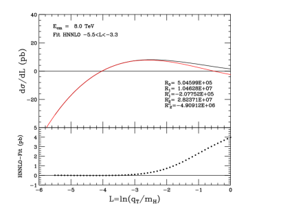
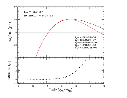
Figure 1: Upper panels: fits to the logarithmic terms of the transverse-momentum ($q_{T}$) distribution in Higgs boson production at the LHC at 8 and 14 TeV. Black: NLO data from HNNLO. Red: fit to data at $-5.5<L<-3.3$. Lower panels: difference between the NLO data and the fits.

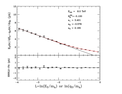
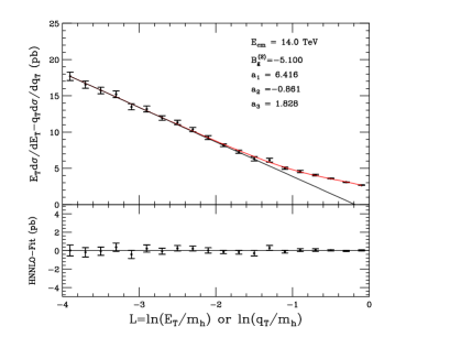
Figure 2: Upper panels: fits to the difference between the transverse-energy ($E_{T}$) and transverse-momentum ($q_{T}$) distribution in Higgs boson production at the LHC at 8 and 14 TeV. Points: NLO data from HNNLO. Red: fit to data. Black: logarithmic terms only. Lower panels: difference between the NLO data and the fits.

3.2 Matching to NLO

The NLO prediction for the transverse-energy distribution is conveniently obtained from the known NLO transverse-momentum distribution by adding the difference between the two distributions, obtained from Higgs plus two-jet production at leading order. Given the value of $B_{g}^{(2)}$ for the transverse-energy distribution, the NLO prediction (80) for the difference at small $E_{T}$ is independent of the fitted parameters $R^{\prime}_{2},R^{\prime\prime}_{2}$. From HNNLO [28, 29] data on this quantity at 8 and 14 TeV, shown in Fig. 2, we find consistent best-fit $B_{g}^{(2)}$ values of $-4.5\pm 2.1$ and $-6.0\pm 2.6$, respectively, with weighted average $B_{g}^{(2)}=-5.1\pm 1.6$. This is significantly different from the value of $\overline{B}_{g}^{(2)}=26.8$ given by Eqs. (2) for the transverse-momentum distribution. We will use $B_{g}^{(2)}=-5.1$ from now on.

Away from the small-$E_{T}$ region, the NLO data are then well described by a parametrization of the form

$$\left[\frac{d\sigma_{H}}{dE_{T}}-\left.\frac{d\sigma_{H}}{dq_{T}}\right|_{q_{T}=E_{T}}\right]_{\rm NLO}=\mbox{Logarithmic terms}+\frac{a_{1}E_{T}}{m_{H}(m_{H}+a_{2}E_{T})+a_{3}E_{T}^{2}}\,,$$ (52)

as shown by the red curves in Fig. 2, with the parameter values shown.

To match the resummed and NLO $E_{T}$ distributions, we have to subtract the NLO logarithmic terms (50), which are already included in the resummation, and replace them by the full NLO result:

$$\frac{d\sigma_{H}}{dE_{T}}=\left[\frac{d\sigma_{H}}{dE_{T}}\right]_{\rm resum}-\left[\frac{d\sigma_{H}}{dE_{T}}\right]_{\rm resum,NLO}+\left[\frac{d\sigma_{H}}{dE_{T}}\right]_{\rm NLO}\,.$$ (53)

3.3 Results

In the following we present numerical results for our resummed calculation of the $E_{T}$ distribution at the LHC. Our resummed results are obtained by using Eq. (53): the resummed component is evaluated by including the coefficients $C_{ga}^{(1)}$ in Eq. (2), and the functions $g_{1}$, $g_{2}$ and $g_{3}$ of Eqs. (2.1). The required coefficients $A_{g}^{(1)}$, $A_{g}^{(2)}$ and $B_{g}^{(1)}$ are given in Eq. (2). For the coefficient $B_{g}^{(2)}$ we use the numerical value extracted in Sec. 3.2. The unknown coefficient $A_{g}^{(3)}$ is neglected. We will comment later on the numerical impact of the missing $A_{g}^{(3)}$ and $C_{ga}^{(2)}$ coefficients.

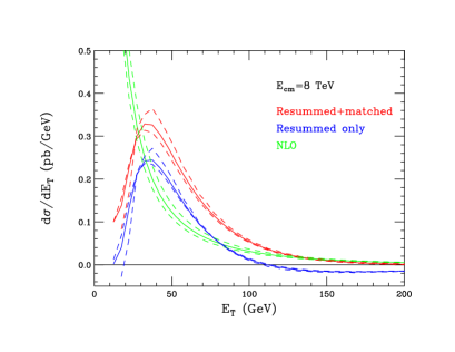
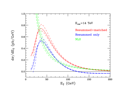
Figure 3: Transverse-energy distribution in Higgs boson production at the LHC at 8 and 14 TeV. Blue: resummed only. Red: resummed and matched to NLO. Green: NLO only. The solid curves correspond to renormalization scale $m_{H}$, the dashed to $2m_{H}$ and $m_{H}/2$.

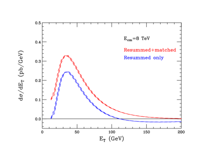
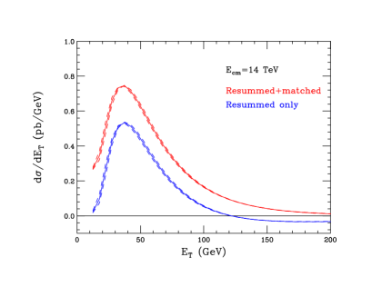
Figure 4: Transverse-energy distribution in Higgs boson production at the LHC at 8 and 14 TeV. Blue: resummed only. Red: resummed and matched to NLO. The solid curves correspond to $A_{g}^{(3)}=0$, the dashed to $A_{g}^{(3)}=\pm 30$.

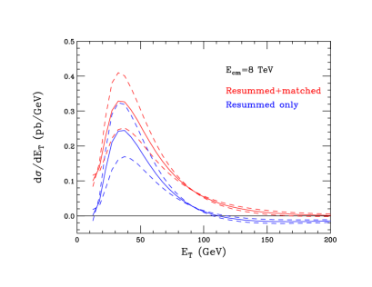
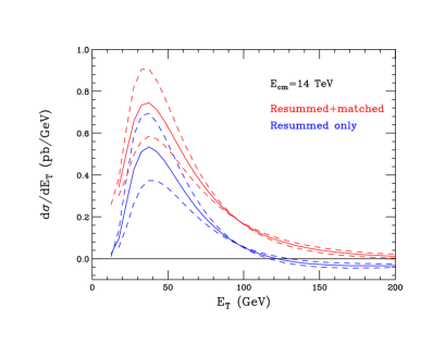
Figure 5: Transverse-energy distribution in Higgs boson production at the LHC at 8 and 14 TeV. Blue: resummed only. Red: resummed and matched to NLO. The solid curves correspond to $C_{g}^{(2)}=0$, the dashed to $C_{g}^{(2)}=\pm 115.5$ (see text).

The resulting resummed and matched $E_{T}$ distributions at the LHC at 8 and 14 TeV are shown in Fig. 3. For all these predictions we use the best-fit value $B_{g}^{(2)}=-5.1$ found from the NLO data. The distribution peaks at around $E_{T}=35$ GeV at both centre-of-mass energies, considerably above the peak in the Higgs transverse-momentum distribution, around $q_{T}=12$ GeV [11]. Thus in the peak region of $E_{T}$ the resummed logarithms are not so dominant as in the corresponding region of $q_{T}$. On the other hand, the fixed-order NLO prediction is rising rapidly and unphysically towards smaller values of $E_{T}$.

The purely resummed distribution becomes slightly negative at small and large $E_{T}$, which is also unphysical. The effect of matching is to raise the distribution to positive values, close to the fixed-order prediction at high $E_{T}$. The matched prediction is still somewhat unstable at small $E_{T}$, owing to the delicate cancellation of diverging logarithmic terms. The behaviour at large $E_{T}$ has been significantly improved compared to the results of Ref. [3] where matching was only performed to leading order. The renormalization scale dependence is comparable to that of the NLO result above and around the peak of the distribution, but changes sign at lower $E_{T}$, with smaller scales giving a lower cross section there and a peak that is higher and shifted to slightly larger $E_{T}$.

As a result of the unitarity condition (36) and the matching to fixed order, the cross section integrated over all $E_{T}$ should be equal to the NNLO inclusive Higgs cross section, within the uncertainties due to the unknown coefficients. Integrating up to $E_{T}=760$ GeV, we obtain resummed matched cross sections of 18.4 pb and 47.8 pb at 8 and 14 TeV, respectively, which compare well with the NNLO inclusive values of 18.22 pb and 47.28 pb, computed with the same NLO PDFs and two-loop $\alpha_{\mathrm{S}}$.

As mentioned above, the leading terms that are neglected in our analysis correspond to the coefficient $A_{g}^{(3)}$ in Eq. (6) and the coefficient functions $C_{ga}^{(2)}(z)$ in (8). In Fig. 4 we show the sensitivity of the prediction to $A_{g}^{(3)}$, assuming a value similar in magnitude to that used for the $q_{T}$ distribution in Ref. [11]. As was found there, the effect of including this coefficient is small.

The NNLO coefficient functions $C^{(2)}_{ga}(z)$ were computed for the Higgs transverse-momentum distribution in Ref. [30], where it was found that their dominant effect could be approximated as

$${\overline{C}}^{(2)}_{ga}(z)\approx{\overline{C}}^{(2)}_{g}\delta_{ag}\,\delta(1-z)$$ (54)

where ${\overline{C}}^{(2)}_{g}=115.5$. In Fig. 5 we show the effects of assuming the same form and magnitude for the corresponding coefficient in $E_{T}$ resummation. We see that the effect is larger than that of $A_{g}^{(3)}$ and of renormalization scale variation. Thus in this case uncertainties in the higher-order coefficient functions provide a more conservative error estimate that the usual range of scale variation.

4 Monte Carlo studies

Up to this point we have only considered the perturbative contributions to the $E_{T}$ distribution that arise due to initial state radiation (ISR). However, there are important contributions to the $E_{T}$ originating from non-perturbative effects such as hadronization and the underlying event (UE). Moreover, the distributions can be altered further because of cuts imposed either due to the detector geometry, or to accommodate the experimental analyses.

All of the aforementioned effects on the $E_{T}$ distribution are challenging to predict analytically. Therefore, we make the assumption that the kinematics of the process, apart from the UE, is governed predominantly by the shape of the $E_{T}$ distribution. Under this assumption, one can reweight the parton-level $E_{T}$ of a Monte Carlo event generator (i.e. with the UE and hadronization turned off), to the one calculated analytically, and use the phenomenogical models of the Monte Carlo to estimate the features of the effects.

Taking into account the non-perturbative and detector geometry effects, one may construct a quantity that is, at least in principle, close to what can be measured experimentally:

$$E_{T}=\sum_{\begin{subarray}{c}|\eta_{i}|<\eta^{c}\\ |\mathbf{p}_{Ti}|>p_{T}^{c}\end{subarray}}|\mathbf{p}_{Ti}|\;,$$ (55)

where the sum is taken over the hadrons in the event, with $p_{T}^{c}$ and $\eta^{c}$ their minimum transverse momentum and maximum pseudorapidity respectively. The effect of these cuts will be investigated below.

4.1 $E_{T}$ at parton level

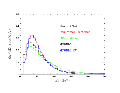
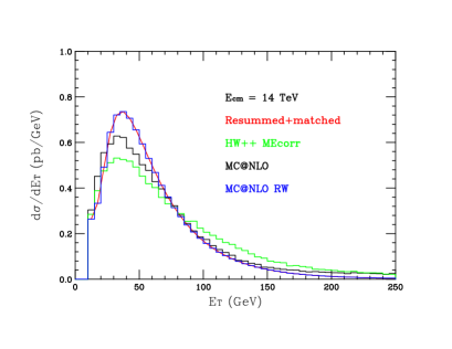
Figure 6: Parton-level transverse-energy distribution in Higgs boson production at the LHC at 8 and 14 TeV. Red: resummed and matched to NLO. Green: Herwig++ with Matrix Element correction, no reweighting. Black: aMC@NLO+Herwig++ before reweighting. Blue: aMC@NLO+Herwig++ after reweighting.

Here we employ the Herwig++ general-purpose event generator (version 2.6.3) [31, 32] in conjunction with events generated using aMC@NLO [33, 34]. For purposes of comparison with alternative descriptions of the parton shower, hadronization and the underlying event, we additionally verify the Herwig++ results using the Pythia8 event generator [35, 36]. The distributions found using Pythia8 are very similar to those obtained with Herwig++ and thus we defer them to Appendix D.

Use of aMC@NLO ensures correct treatment of the NLO inclusive cross section matched to parton showers without double counting. We assign a new weight to each event so as to reproduce the analytic resummed and matched distributions shown in Fig. 3. For completeness, we show in Fig. 6 the resulting $E_{T}$ distributions before and after the reweighting, at parton level, demonstrating that this procedure reproduces the analytic result. Higgs boson production using the internal Herwig++ implementation, which includes Matrix Element (ME) corrections, is also shown on the figure. The ME-corrected $E_{T}$ distribution has a lower peak and consequently falls off more slowly at higher $E_{T}$ than the MC@NLO case. In Fig. 7 we show the Higgs boson transverse-momentum distribution, $q_{T}$, before and after applying the reweighting procedure, compared to the equivalent distribution obtained by the HQT program [11, 37]. Evidently, the MC@NLO distribution agrees already quite well with the HQT prediction before reweighting. The reweighting procedure improves agreement in the peak region but makes the distribution fall off faster at high $q_{T}$, which is consistent with the change in shape observed in Fig. 6. Figure 8 shows the rapidity distribution of the Higgs boson, $y_{H}$, before and after the reweighting, clearly showing that the effect on this distribution is negligible, thus verifying that the reweighting does not alter physics in the forward direction.

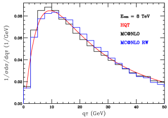
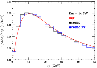
Figure 7: Higgs boson transverse-momentum distribution at the LHC at 8 and 14 TeV. Red: HQT calculation. Black: aMC@NLO+Herwig++ before reweighting. Blue: aMC@NLO+Herwig++ after reweighting.

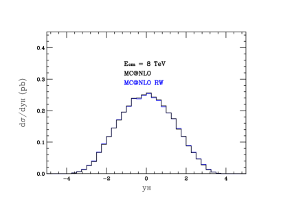
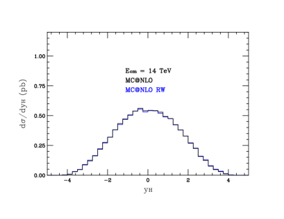
Figure 8: Higgs boson rapidity distribution at the LHC at 8 and 14 TeV. Black: aMC@NLO+Herwig++ before reweighting. Blue: aMC@NLO+Herwig++ after reweighting.

4.2 $E_{T}$ at hadron level

The effects of hadronization can be studied by enabling the cluster hadronization model in the Herwig++ event generator in conjunction with the reweighting. The default parameters of the hadronization model available in Herwig++  version 2.6.3 were used. The effect is to shift the peak of the distribution to higher $E_{T}$, by about 15 GeV at both 8 TeV and 14 TeV, as shown in Fig. 9. The effect of hadronization on the $E_{T}$ distribution can be compensated almost completely in this range of values by imposing a pseudorapidity cut on the hadrons contributing to the $E_{T}$, allowing only hadrons within $|\eta|<5$ to enter. The resulting distributions after this cut are also shown in Fig. 9. We note that including the restriction on hadrons of $|\eta|<5$ approximately corresponds to the experimental detector coverage of the ATLAS and CMS detectors.

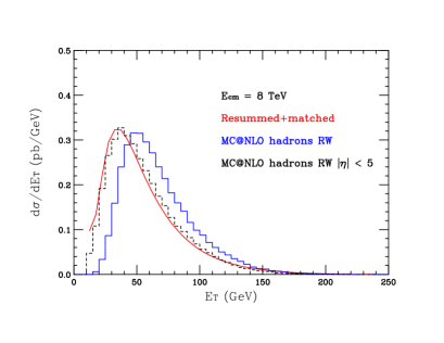
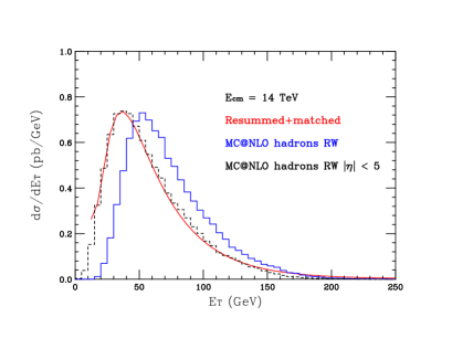
Figure 9: Hadron-level transverse-energy distribution in Higgs boson production at the LHC at 8 and 14 TeV. Red: resummed and matched to NLO. Blue: aMC@NLO+Herwig++ after reweighting. Black dashes: aMC@NLO+Herwig++ after reweighting, particles restricted to lie within pseudorapidity $|\eta|<5$.

4.3 Inclusion of the underlying event

The underlying event (UE) is thought to arise due to secondary multiple interactions between the colliding hadrons. The model present in Herwig++ is based on the eikonal model formulated in Refs. [38, 39, 40]. The underlying event activity is treated as additional semi-hard and soft partonic scatters. In this version, a model of colour reconnection has been added to HERWIG++, based on the idea of colour preconfinement, which provides an improved description of underlying event data at the LHC [41].

The effect of the UE on the $E_{T}$ distributions is severe, making them much broader and moving the peak to much higher values of $E_{T}$. This was investigated in Ref. [3] at parton level, where it was shown that in the Herwig++ model the $E_{T}$ distribution for the partons originating from the UE is approximately independent of the nature of the hard process. This distribution was fitted with a Fermi distribution and was shown to reproduce the total distribution after convolution with the perturbative result.

We present results using the default parameters present in Herwig++ version 2.6.3 for the underlying event model. We note that these were tuned to a variety of experimental data using the MRST LO** PDF set [42] instead of the MSTW2008 NLO set [27] used here for the hard process generated using aMC@NLO. In Fig. 10 we show the $E_{T}$ distribution including the UE, with hadrons of a maximum pseudorapidity $\eta^{c}=5$, compared against the analytical result, which we have shown matches well the hadron-level $\eta^{c}=5$ distribution without UE (Fig. 9). In practice, particles cannot be detected at transverse momenta down to zero, and therefore we show the effect of applying transverse-momentum cuts on the hadrons: $p_{T}^{c}=1.0,1.5,2.0$ GeV. When $p_{T}^{c}=1.5$ GeV the peak in $E_{T}$ is moved back to approximately the value of the parton-level prediction, but the distribution itself is still somewhat broader.

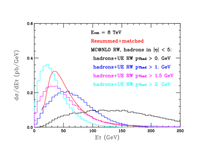
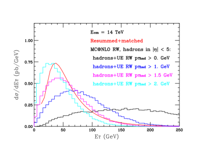
Figure 10: Hadron-level transverse-energy distribution in Higgs boson production at the LHC at 8 and 14 TeV, including the effect of the underlying event. Red: resummed and matched to NLO, for comparison. Reweighted aMC@NLO+Herwig++ events with hadron maximum pseudorapidity $\eta^{c}=5$: Black: $p_{T}^{c}=0$ GeV, Blue: $p_{T}^{c}=1.0$ GeV, Magenta: $p_{T}^{c}=1.5$ GeV, Cyan: $p_{T}^{c}=2.0$ GeV.

We have also investigated the impact of the underlying event using different PDFs and different, reasonable, model parameters. We found that, with reasonably-tuned values for the underlying event model parameters, the change of PDF sets does not induce any significant changes to the distributions.

To conclude, one can reproduce the $E_{T}$ distribution with the effect of the UE and detector geometry effects by reweighting the parton-level Monte Carlo events to match the analytical prediction of the $E_{T}$ due to ISR and subsequently enabling the hadronization and underlying event models of the generator. The description of the underlying event is robust against changes of tune parameters as well as PDF sets. However, in the presence of the underlying event the $E_{T}$ distribution is highly sensitive to the minimum hadron transverse momentum, $p_{T}^{c}$.

5 Conclusions

We have presented the first detailed predictions of the transverse-energy distribution in Higgs boson production at the LHC ($\sqrt{s}=8$ and $14$ TeV) for $m_{H}=126$ GeV. Our calculation includes the resummation of the large logarithmic terms at small $E_{T}$ up to (almost) NNLL accuracy, matched to the fixed-order NLO result in a way that limits the impact of the resummation in the intermediate and large-$E_{T}$ regions.

Our main result for the resummation is Eq. (35), with component expressions (13), (2.1) and (30). For the matching we have Eq. (53) with (3.1), (50) and (3.1). The resulting predictions are shown in Fig. 3. The effect of resummation, compared to the pure NLO result, is large over the whole range of $E_{T}$. The purely resummed distribution peaks at around 35 GeV and falls to unphysical negative values at small and large $E_{T}$. This behaviour is rectified by matching, which also provides the NNLO normalization, without shifting the peak significantly. The uncertainty in the prediction, as assessed by the customary factor-of-two variation of the renormalization scale, is of the order of $\pm 10\%$. However, the sensitivity to unknown terms beyond NLO, in particular the NNLO coefficient function $C^{(2)}_{g}$, is considerable, suggesting a larger uncertainty. The possible impacts of $C_{g}^{(2)}$ and the neglected NNLL coefficient $A_{g}^{(3)}$ were illustrated in Figs. 5 and 4 respectively.

The resummed and matched predictions refer only to the perturbative hard-scattering component of Higgs production. In real events there are the non-perturbative effects of hadronization and the underlying event. We made a Monte Carlo study of these effects using aMC@NLO interfaced to Herwig++ or Pythia8, which provide a state-of-the-art simulation of complete LHC final states. The simulated events were reweighted at the parton level to reproduce the analytically resummed and matched $E_{T}$ distribution. The effect of hadronization was to shift the peak of the distribution upwards, to around 50 GeV, if all produced hadrons were included. However, this effect was practically eliminated by a pseudorapidity cut $|\eta_{\rm had}|<5$. The effect of the underlying event was much greater, even in the presence of the pseudorapidity cut, the $E_{T}$ distribution becoming much broader, as was found in Ref. [3]. This effect is due to soft hadrons in the underlying event; a cut on hadron transverse momenta $p_{T{\rm had}}>1.5$ GeV restored the $E_{T}$ peak to around 30-40 GeV, although with a distribution still somewhat broader than the parton-level prediction.

Measurements of differential distributions of the Higgs boson at the LHC are starting to appear [44]. We look forward to measurement of the transverse-energy distribution and to comparisons with our theoretical predictions.

Appendix A Proof of an identity

To prove Eq. (28), we will show in general that

$$\left.f\left(\frac{d}{du}\right)\frac{Z(u)}{u}\left[{\rm e}^{\lambda u}-1\right]\right|_{u=0}=\left.Z\left(\frac{d}{d\lambda}\right)f\left(\frac{d}{du}\right)\frac{1}{u}\left[{\rm e}^{\lambda u}-1\right]\right|_{u=0}\,,$$ (56)

where $f$ and $Z$ have power series expansions,

$$f(x)=\sum_{\ell}f_{\ell}\,x^{\ell}\,,\;\;\;Z(u)=\sum_{m}Z_{m}\,u^{m}\,,$$ (57)

which holds for the functions in Eq. (28). Now, beginning with the left-hand side,

$$\frac{1}{u}\left[{\rm e}^{\lambda u}-1\right]=\sum_{n=0}^{\infty}\frac{\lambda^{n+1}}{(n+1)!}u^{n}\,,$$ (58)

so we can write

$$\left.f\left(\frac{d}{du}\right)\frac{Z(u)}{u}\left[{\rm e}^{\lambda u}-1\right]\right|_{u=0} = \sum_{\ell mn}\left.f_{\ell}\,Z_{m}\frac{d^{\ell}}{du^{\ell}}\frac{\lambda^{n+1}}{(n+1)!}u^{m+n}\right|_{u=0}$$

$$= \sum_{\ell mn}f_{\ell}\,Z_{m}\lambda^{n+1}\frac{(m+n)!}{(n+1)!}\,\delta_{\ell-m-n}$$

$$= \sum_{\ell m}f_{\ell}\,Z_{m}\lambda^{\ell-m+1}\frac{\ell!}{(\ell-m+1)!}$$

$$= \sum_{\ell m}f_{\ell}\,Z_{m}\frac{d^{m}}{d\lambda^{m}}\frac{\lambda^{\ell+1}}{(\ell+1)}$$

$$= \left.Z\left(\frac{d}{d\lambda}\right)f\left(\frac{d}{du}\right)\frac{1}{u}\left[{\rm e}^{\lambda u}-1\right]\right|_{u=0}\,.$$

Appendix B Dispersion relations

The fact that $d\sigma/dE_{T}\equiv F(E_{T})$ has to vanish for $E_{T}<0$ implies that its Fourier transform $G(\tau)$ must satisfy dispersion relations analogous to those in the frequency domain that follow from causality. Note first that if we write

$$F(E_{T})=\Theta(E_{T})f(E_{T})\,,$$ (60)

where $\Theta$ is the Heaviside step-function, then $f(E_{T})$ can be chosen to be either an odd or an even function. We choose $f$ even, and then its Fourier transform $g(\tau)$ is purely real. Now the Fourier transform of a product is a convolution, so

$$G(\tau)=\frac{1}{2\pi}\int_{-\infty}^{+\infty}d\tau^{\prime}\,h(\tau-\tau^{\prime})g(\tau^{\prime})$$ (61)

where $h$ is the Fourier transform of $\Theta$:

$$h(\tau)=\pi\,\delta(\tau)+P\frac{i}{\tau}\,,$$ (62)

$P$ indicating the principal value. Thus

$$G(\tau)=\frac{1}{2}g(\tau)+\frac{i}{2\pi}P\int_{-\infty}^{+\infty}d\tau^{\prime}\,\frac{g(\tau^{\prime})}{\tau-\tau^{\prime}}\,.$$ (63)

Now writing $G=G_{R}+iG_{I}$, recalling that $g(\tau)$ is real and equating real parts we see that

$$g(\tau)=2G_{R}(\tau)\,.$$ (64)

Furthermore $G_{I}$ is not an independent function: it must satisfy the dispersion relation

$$G_{I}(\tau)=\frac{1}{\pi}P\int_{-\infty}^{+\infty}d\tau^{\prime}\,\frac{G_{R}(\tau^{\prime})}{\tau-\tau^{\prime}}\,.$$ (65)

Notice that it follows that $G_{R}(\tau)$ must be an even function while $G_{I}(\tau)$ must be odd, i.e. $G(-\tau)=G^{*}(\tau)$. Altogether, we have

$$G(\tau)=G_{R}(\tau)+\frac{i}{\pi}P\int_{-\infty}^{+\infty}d\tau^{\prime}\,\frac{G_{R}(\tau^{\prime})}{\tau-\tau^{\prime}}\,.$$ (66)

Thus

$$F(E_{T})=\frac{1}{2\pi}\int_{-\infty}^{+\infty}d\tau\,{\rm e}^{-iE_{T}\tau}\left[G_{R}(\tau)+\frac{i}{\pi}P\int_{-\infty}^{+\infty}d\tau^{\prime}\,\frac{G_{R}(\tau^{\prime})}{\tau-\tau^{\prime}}\right]\,.$$ (67)

Assuming that the order of integration can be exchanged, the second term involves

$$I(\tau^{\prime})\equiv\frac{i}{\pi}P\int_{-\infty}^{+\infty}d\tau\,\frac{{\rm e}^{-iE_{T}\tau}}{\tau-\tau^{\prime}}\,.$$ (68)

The principal value implies the average of integrations along contours above and below the pole at $\tau=\tau^{\prime}$. The contour can be closed in the lower half-plane, where the exponential vanishes at infinity since $E_{T}>0$. Thus

$$I(\tau^{\prime})={\rm e}^{-iE_{T}\tau^{\prime}}$$ (69)

and, relabelling $\tau^{\prime}$ as $\tau$ in the second term, we see that the two terms are equal and

$$F(E_{T})=\frac{1}{\pi}\int_{-\infty}^{+\infty}d\tau\,{\rm e}^{-iE_{T}\tau}G_{R}(\tau)\,.$$ (70)

Thus we can simply replace the full Fourier transform $G$ by twice its real part. Furthermore, since $G_{R}$ is an even function, it then follows immediately that

$$\int_{0}^{\infty}F(E_{T})\,dE_{T}=G_{R}(0)\,.$$ (71)

In the notation of Eq. (35), we have

$$G_{R}(\tau)={\rm e}^{-F_{g}^{(R)}(Q,\tau)} \Bigl{[} R_{g}^{(R)}(s;Q,\tau)\cos\{F_{g}^{(I)}(Q,\tau)\}$$ (72)

$$- \,R_{g}^{(I)}(s;Q,\tau)\sin\{F_{g}^{(I)}(Q,\tau)\}\;\Bigr{]}\,\sigma_{gg}^{H}(Q,\alpha_{\mathrm{S}}(Q))$$

and, by virtue of the shift (32), $F_{g}^{(R)}(Q,0)=F_{g}^{(I)}(Q,0)=0$, so we obtain Eq. (36).

Appendix C Comparison with transverse-momentum resummation

For the Higgs transverse momentum $q_{T}$, instead of integrals of the form (43) we have

$$\overline{\cal I}_{p}(q_{T},Q)=q_{T}\int_{0}^{\infty}db\,bJ_{0}(bq_{T})\ln^{p}\left(\frac{bQ}{b_{0}}\right)\;,$$ (73)

where $b_{0}=2\exp(-\gamma_{\rm E})$. These integrals may be evaluated from

$$\overline{\cal I}_{p}(q_{T},Q)=\frac{d^{p}}{du^{p}}\overline{\cal I}(q_{T},Q;u)|_{u=0}$$ (74)

where

$$\overline{\cal I}(q_{T},Q) = q_{T}\int_{0}^{\infty}db\,bJ_{0}(bq_{T})\left(\frac{bQ}{b_{0}}\right)^{u}$$ (75)

$$= -\frac{2{\rm e}^{u\gamma_{\rm E}}}{\pi q_{T}}\left(\frac{Q}{q_{T}}\right)^{u}\sin\left(\frac{\pi u}{2}\right)\Gamma^{2}\left(1+\frac{u}{2}\right)\;,$$

which can be written as

$$\overline{\cal I}(q_{T},Q) = -\frac{u{\rm e}^{u\gamma_{\rm E}}}{q_{T}}\left(\frac{Q}{q_{T}}\right)^{u}\frac{\Gamma(1+u/2)}{\Gamma(1-u/2)}$$ (76)

$$= -\frac{u}{q_{T}}\left(\frac{Q}{q_{T}}\right)^{u}\exp\left[-2\sum_{k=1}^{\infty}\frac{\zeta_{2k+1}}{2k+1}\left(\frac{u}{2}\right)^{2k+1}\right]\;.$$

This gives instead of Eq. (3.1)

$$\overline{\cal I}_{1}(q_{T},Q) = -\frac{1}{q_{T}}\;,\quad\overline{\cal I}_{2}(q_{T},Q)=-\frac{2}{q_{T}}\ln\left(\frac{Q}{q_{T}}\right)$$

$$\overline{\cal I}_{3}(q_{T},Q) = -\frac{3}{q_{T}}\ln^{2}\left(\frac{Q}{q_{T}}\right)$$

$$\overline{\cal I}_{4}(q_{T},Q) = -\frac{4}{q_{T}}\left[\ln^{3}\left(\frac{Q}{q_{T}}\right)-\frac{1}{2}\zeta_{3}\right]\;.$$ (77)

Therefore at small $q_{T}>0$ we expect

$$\left[\frac{q_{T}}{\sigma_{0}^{H}}\frac{d\sigma_{H}}{dq_{T}}\right]_{\rm NLO}\sim a_{R}(\overline{G}_{0}R_{0}+\overline{G}^{\prime}_{1}R^{\prime}_{1})+a_{R}^{2}(\overline{H}_{0}R_{0}+\overline{H}_{1}R_{1}+\overline{H}^{\prime}_{1}R^{\prime}_{1}+\overline{H}^{\prime}_{2}R^{\prime}_{2}+\overline{H}^{\prime\prime}_{2}R^{\prime\prime}_{2})$$ (78)

where, writing $L=\ln(Q/q_{T})$,

$$\overline{G}_{0} = \overline{H}_{1}=4A_{g}^{(1)}L+2B_{g}^{(1)}\;,\;\;\;\overline{G}^{\prime}_{1}=-1\;,$$

$$\overline{H}_{0} = 4L\left[A_{g}^{(2)}+\beta_{0}B_{g}^{(1)}-\beta_{0}A_{g}^{(1)}\ln\left(\frac{Q^{2}}{\mu_{R}^{2}}\right)\right]+8\beta_{0}A_{g}^{(1)}L^{2}$$

$$+ 2\left[\overline{B}_{g}^{(2)}-\beta_{0}B_{g}^{(1)}\ln\left(\frac{Q^{2}}{\mu_{R}^{2}}\right)\right]-8(A_{g}^{(1)})^{2}\left(L^{3}-\frac{1}{2}\zeta_{3}\right)$$

$$- 12A_{g}^{(1)}B_{g}^{(1)}L^{2}-4(B_{g}^{(1)})^{2}L\;,$$

$$\overline{H}^{\prime}_{1} = 6A_{g}^{(1)}L^{2}+4B_{g}^{(1)}L\;,$$

$$\overline{H}^{\prime}_{2} = -1\;,\;\;\;\overline{H}^{\prime\prime}_{2}=-2L\;.$$ (79)

Here we have allowed for the possibility that the coefficient $\overline{B}_{g}^{(2)}$ for $q_{T}$ may be different from $B_{g}^{(2)}$ for $E_{T}$. Comparing with Eqs. (50) and (3.1), we see that the NLO $E_{T}$ and $q_{T}$ distributions at the point $q_{T}=E_{T}$ differ by

$$\frac{d\sigma_{H}}{dE_{T}}-\left.\frac{d\sigma_{H}}{dq_{T}}\right|_{q_{T}=E_{T}}\sim\;\;a_{R}^{2}\,\frac{\sigma_{B}^{H}}{E_{T}}\left[H_{0}-\overline{H}_{0}+(H^{\prime}_{1}-\overline{H}^{\prime}_{1})\frac{R^{\prime}_{1}}{R_{0}}\right]$$ (80)

where $\sigma_{B}^{H}=\sigma_{0}^{H}R_{0}$ is the Born cross section and

$$H_{0}-\overline{H}_{0} = \frac{4}{3}\pi^{2}A_{g}^{(1)}\left(2A_{g}^{(1)}L+B_{g}^{(1)}\right)+2\left(B_{g}^{(2)}-\overline{B}_{g}^{(2)}\right)+12\zeta_{3}\left(A_{g}^{(1)}\right)^{2}\,,$$

$$H^{\prime}_{1}-\overline{H}^{\prime}_{1} = -\frac{2}{3}\pi^{2}A_{g}^{(1)}\,.$$ (81)

Appendix D Alternative Monte Carlo results

For purposes of comparison with alternative descriptions of the parton shower, hadronization and the underlying event, we provide here results equivalent to those obtained using Herwig++ in Sec. 4, using the Pythia8 event generator [35, 36]. We use the default parameters appearing in Pythia8  version 8.185, with the Higgs boson mass set to 126 GeV. Figure 11 is equivalent to Fig. 6 for Herwig++ and demonstrates that the reweighting procedure reproduces the analytical resummed and matched result.

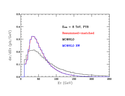
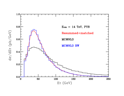
Figure 11: Parton-level transverse-energy distribution in Higgs boson production at the LHC at 8 and 14 TeV. Red: resummed and matched to NLO. Black: aMC@NLO+Pythia8 before reweighting. Blue: aMC@NLO+Pythia8 after reweighting.

In Fig. 12 we show the effect of hadronization on the parton-level $E_{T}$ distribution. Comparing to Fig. 9, it can be observed that the effect is of similar magnitude and the compensation obtained by applying a cut of $|\eta|<5$ persists in Pythia8.

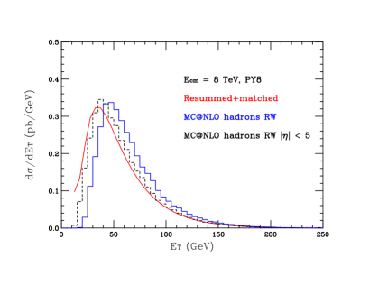
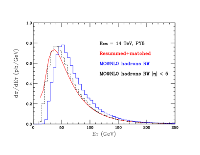
Figure 12: Hadron-level transverse-energy distribution in Higgs boson production at the LHC at 8 and 14 TeV. Red: resummed and matched to NLO. Blue: aMC@NLO+Pythia8. Black dashes: aMC@NLO+Pythia8  particles restricted to lie within pseudorapidity $|\eta|<5$.

The effect of the underlying event model present in Pythia8 is shown in Fig. 13. Evidently, the effect is qualitatively similar to what was shown in Fig. 10 for Herwig++. Moreover, the effect of imposing a minimum transverse momentum on the contributing hadrons is also identical to that observed in Herwig++.

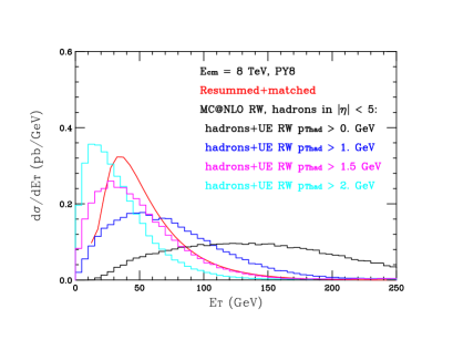
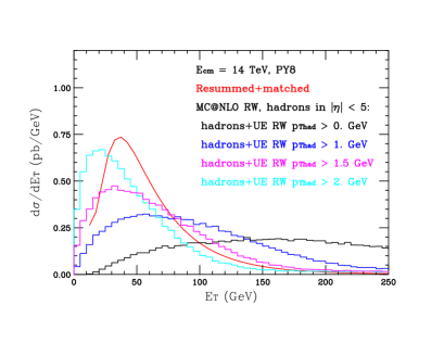
Figure 13: Hadron-level transverse-energy distribution in Higgs boson production at the LHC at 8 and 14 TeV, including the effect of the underlying event. Red: resummed and matched to NLO. aMC@NLO+Pythia8 events with hadron maximum pseudorapidity $\eta^{c}=5$: Black: $p_{T}^{c}=0$ GeV, Blue: $p_{T}^{c}=1.0$ GeV, Magenta: $p_{T}^{c}=1.5$ GeV, Cyan: $p_{T}^{c}=2.0$ GeV.

References

- [1] G. Aad et al. [ATLAS Collaboration], Phys. Lett. B 716 (2012) 1 [arXiv:1207.7214 [hep-ex]].
- [2] S. Chatrchyan et al. [CMS Collaboration], Phys. Lett. B 716 (2012) 30 [arXiv:1207.7235 [hep-ex]].
- [3] A. Papaefstathiou, J. M. Smillie and B. R. Webber, JHEP 1004 (2010) 084 [arXiv:1002.4375 [hep-ph]].
- [4] F. Halzen, A. D. Martin, D. M. Scott and M. P. Tuite, Z. Phys. C 14 (1982) 351.
- [5] C. T. H. Davies and B. R. Webber, Z. Phys. C 24 (1984) 133.
- [6] G. Altarelli, G. Martinelli and F. Rapuano, Z. Phys. C 32 (1986) 369.
- [7] G. Parisi and R. Petronzio, Nucl. Phys. B154 (1979) 427.
- [8] J. C. Collins, D. E. Soper and G. Sterman, Nucl. Phys. B 250 (1985) 199.
- [9] G. Bozzi, S. Catani, G. Ferrera, D. de Florian and M. Grazzini, Phys. Lett. B 696 (2011) 207 [arXiv:1007.2351 [hep-ph]].
- [10] T. Becher and M. Neubert, Eur. Phys. J. C 71 (2011) 1665 [arXiv:1007.4005 [hep-ph]].
- [11] G. Bozzi, S. Catani, D. de Florian and M. Grazzini, Nucl. Phys. B 737 (2006) 73 [hep-ph/0508068].
- [12] G. Bozzi, S. Catani, D. de Florian and M. Grazzini, Nucl. Phys. B 791 (2008) 1 [arXiv:0705.3887 [hep-ph]].
- [13] S. Mantry and F. Petriello, Phys. Rev. D 81 (2010) 093007 [arXiv:0911.4135 [hep-ph]].
- [14] S. Catani and M. Grazzini, Nucl. Phys. B 845 (2011) 297 [arXiv:1011.3918 [hep-ph]].
- [15] A. Banfi, G. P. Salam and G. Zanderighi, JHEP 1206 (2012) 159 [arXiv:1203.5773 [hep-ph]].
- [16] T. Becher and M. Neubert, JHEP 1207 (2012) 108 [arXiv:1205.3806 [hep-ph]].
- [17] A. Banfi, P. F. Monni, G. P. Salam and G. Zanderighi, Phys. Rev. Lett. 109 (2012) 202001 [arXiv:1206.4998 [hep-ph]].
- [18] T. Becher, M. Neubert and L. Rothen, JHEP 1310 (2013) 125 [arXiv:1307.0025 [hep-ph]].
- [19] I. W. Stewart, F. J. Tackmann, J. R. Walsh and S. Zuberi, arXiv:1307.1808.
- [20] S. Catani, D. de Florian and M. Grazzini, Nucl. Phys. B 596, 299 (2001) [arXiv:hep-ph/0008184].
- [21] S. Catani, E. D’Emilio and L. Trentadue, Phys. Lett. B211 (1988) 335.
- [22] R. P. Kauffman, Phys. Rev. D45 (1992) 1512.
- [23] D. de Florian and M. Grazzini, Phys. Rev. Lett. 85 (2000) 4678 [arXiv:hep-ph/0008152].
- [24] D. de Florian and M. Grazzini, Nucl. Phys. B 616 (2001) 247 [arXiv:hep-ph/0108273].
- [25] S. Frixione, P. Nason and G. Ridolfi, Nucl. Phys. B 542 (1999) 311 [hep-ph/9809367].
- [26] D. de Florian and M. Grazzini, Nucl. Phys. B 704 (2005) 387 [hep-ph/0407241].
- [27] A. D. Martin, W. J. Stirling, R. S. Thorne and G. Watt, Eur. Phys. J. C 63 (2009) 189 [arXiv:0901.0002 [hep-ph]].
- [28] S. Catani and M. Grazzini, Phys. Rev. Lett. 98 (2007) 222002 [hep-ph/0703012].
- [29] M. Grazzini, JHEP 0802 (2008) 043 [arXiv:0801.3232 [hep-ph]].
- [30] S. Catani and M. Grazzini, Eur. Phys. J. C 72 (2012) 2013 [Erratum-ibid. C 72 (2012) 2132] [arXiv:1106.4652 [hep-ph]].
- [31] M. Bahr et al., Eur. Phys. J. C 58 (2008) 639 [arXiv:0803.0883 [hep-ph]]; arXiv:0812.0529 [hep-ph]. http://projects.hepforge.org/herwig/
- [32] K. Arnold, L. d’Errico, S. Gieseke, D. Grellscheid, K. Hamilton, A. Papaefstathiou, S. Platzer and P. Richardson et al., arXiv:1205.4902 [hep-ph].
- [33] S. Frixione and B. R. Webber, JHEP 0206 (2002) 029 [hep-ph/0204244].
- [34] R. Frederix, S. Frixione, V. Hirschi, F. Maltoni, R. Pittau and P. Torrielli, JHEP 1202 (2012) 099 [arXiv:1110.4738 [hep-ph]].
- [35] T. Sjostrand, S. Mrenna and P. Z. Skands, JHEP 0605 (2006) 026 [hep-ph/0603175].
- [36] T. Sjostrand, S. Mrenna and P. Z. Skands, Comput. Phys. Commun. 178 (2008) 852 [arXiv:0710.3820 [hep-ph]].
- [37] D. de Florian, G. Ferrera, M. Grazzini and D. Tommasini, JHEP 1111 (2011) 064 [arXiv:1109.2109 [hep-ph]].
- [38] L. Durand and H. Pi, Phys. Rev. D 40 (1989) 1436.
- [39] J. M. Butterworth, J. R. Forshaw and M. H. Seymour, Z. Phys. C 72 (1996) 637 [arXiv:hep-ph/9601371]. http://projects.hepforge.org/jimmy/
- [40] I. Borozan and M. H. Seymour, JHEP 0209 (2002) 015 [hep-ph/0207283].
- [41] S. Gieseke, C. Rohr and A. Siodmok, Eur. Phys. J. C 72 (2012) 2225 [arXiv:1206.0041 [hep-ph]].
- [42] A. Sherstnev and R. S. Thorne, Eur. Phys. J. C 55 (2008) 553 [arXiv:0711.2473 [hep-ph]]; arXiv:0807.2132 [hep-ph].
- [43] M. R. Whalley, D. Bourilkov and R. C. Group, hep-ph/0508110.
- [44] The ATLAS collaboration, ATLAS-CONF-2013-072.