Statistical Decision Making for Optimal Budget Allocation in Crowd Labeling

Xi Chen
UC Berkeley
xichen@cs.cmu.edu
   Qihang Lin
University of Iowa
qihang-lin@uiowa.edu
   Dengyong Zhou
Microsoft Research
dengyong.zhou@microsoft.com
Abstract

There is an increasing popularity in crowdsourcing data labeling tasks to non-expert workers or annotators recruited through commercial internet services such as Amazon Mechanical Turk. Those crowdsourcing workers need to be paid for each label they provide, while a task requester usually only has a limited amount of budget for data labeling. So it is desirable to have an optimal policy to wisely allocate the budget among workers and data instances which need to label by considering worker reliability and task difficulty such that the quality of the finally aggregated labels can be maximized. We formulate such a budget allocation problem as a Bayesian Markov decision process (MDP) which simultaneously conducts learning and decision making. Under our framework, the optimal allocation policy can be obtained by applying dynamic programming (DP), but DP quickly becomes computationally intractable when the size of the problem increases. To solve this challenge, we propose a computationally efficient approximate policy called optimistic knowledge gradient policy. Experiments on both synthetic and real data show that at the same budget level our policy results in higher quality labels than existing policies.

1 Introduction

In many machine learning applications, data are usually collected without labels. For example, a digital camera does not automatically tag a picture as a portrait or a landscape. A traditional way for data labeling is to hire a small group of experts to provide labels for the entire set of data. However, for large-scale data, such an approach becomes inefficient and very costly. Thanks to the advent of online crowdsourcing services such as Amazon Mechanical Turk, a much more efficient way is to post unlabeled data to a crowdsourcing marketplace, where a big crowd of low-paid workers can be hired instantaneously to perform labeling tasks.

Despite of its high efficiency and immediate availability, crowd labeling raises many new challenges. Since labeling tasks are tedious and workers are usually non-experts, labels generated by the crowd suffer from low quality. As a remedy, most crowdsourcing services resort to labeling redundancy to reduce the labeling noise, which is achieved by collecting multiple labels from different workers for each data instance. In particular, a crowd labeling process can be described as a two phase procedure:

  1. 1.

    Assign unlabeled data to a crowd of workers and each data instance is asked to label multiple times;

  2. 2.

    Aggregate the collected raw labels to infer the true labels.

In principle, more raw labels will lead to a higher chance of recovering the true label. However, each raw label comes with a cost: the requester has to pay workers pre-specified monetary reward for each label they provide, usually, regardless of the label’s correctness. For example, a worker typically earns 10 cents by categorizing a website as porn or not. In practice, the requester has only a limited amount of budget which essentially restricts the total number of raw labels that he/she can collect. This raises a challenging question central in crowd labeling: What is the best way to allocate the budget among data instances and workers so that the overall accuracy of aggregated labels is maximized ?

The most important factors that decide how to allocate the budget are the intrinsic characteristics of data instances and workers: labeling difficulty/ambiguity for each data instance and reliability/quality of each worker. In particular, an instance is less ambiguous if its label can be decided based on the common knowledge and a vast majority of reliable workers will provide the same label for it. In principle, we should avoid spending too much budget on those easy instances since excessive raw labels will not bring much additional information. In contrast, for an ambiguous instance which falls near the boundary of categories, even those reliable workers will still disagree with each other and generate inconsistent labels. For those ambiguous instances, we are facing a challenging decision problem on how much budget that we should spend on them. On one hand, it is worth to collect more labels to boost the accuracy of the aggregate label. On the other hand, since our goal is to maximize the overall labeling accuracy, when the budget is limited, we should simply put those few highly ambiguous instances aside to save budget for labeling less difficult instances. In addition to the ambiguity of data instances, the other important factor is the reliability of each worker and, undoubtedly, it is desirable to assign more instances to those reliable workers. Despite of their importance in deciding how to allocate the budget, both the data ambiguity and workers’ reliability are unknown parameters at the beginning and need to be updated based on the stream of collected raw labels in an online fashion. This further suggests that the budget allocation policy should be dynamic and simultaneously conduct parameter estimation and decision making.

To search for an optimal budget allocation policy, we model the data ambiguity and workers’ reliability using two sets of random variables drawn from known prior distributions. Then, we formulate the problem into a finite-horizon Bayesian Markov Decision Process (MDP) [29], whose state variables are the posterior distributions of these variables, which are updated by each new label. Here, the Bayesian setting is necessary. We will show that an optimal policy only exists in the Bayesian setting. Using the MDP formulation, the optimal budget allocation policy for any finite budget level can be readily obtained via the dynamic programming (DP). However, DP is computationally intractable for large-scale problems since the size of the state space grows exponentially in budget level. The existing widely-used approximate policies, such as approximate Gittins index rule [12] or knowledge gradient (KG) [13, 9], either has a high computational cost or poor performance in our problem. In this paper, we propose a new policy, called optimistic knowledge gradient (Opt-KG). In particular, the Opt-KG policy dynamically chooses the next instance-worker pair based on the optimistic outcome of the marginal improvement on the accuracy, which is a function of state variables. We further propose a more general Opt-KG policy using the conditional value-at-risk measure [32]. The Opt-KG is computationally efficient, achieves superior empirical performance and has some asymptotic theoretical guarantees.

To better present the main idea of our MDP formulation and the Opt-KG policy, we start from the binary labeling task (i.e., providing the category, either positive or negative, for each instance). We first consider the pull marketplace (e.g., Amazon Mechanical Turk or Galaxy Zoo) , where the labeling requester can only post instances to the general worker pool with either anonymous or transient workers, but cannot assign to an identified worker. In a pull marketplace, workers are typically treated as homogeneous and one models the entire worker pool instead of each individual worker. We further assume that workers are fully reliable (or noiseless) such that the chance that they make an error only depend on instances’ own ambiguity. At a first glance, such an assumption may seem oversimplified. In fact, it turns out that the budget-optimal crowd labeling under such an assumption has been highly non-trivial. We formulate this problem into a Bayesian MDP and propose the computational efficient Opt-KG policy. We further prove that the Opt-KG policy in such a setting is asymptotically consistent, that is, when the budget goes to infinity, the accuracy converges to 100% almost surely.

Then, we extend the MDP formulation to deal with push marketplaces with heterogeneous workers. In a push marketplace (e.g., data annotation team in Microsoft Bing group), once an instance is allocated to an identified worker, the worker is required to finish the instance in a short period of time. Based on the previous model for fully reliable workers, we further introduce another set of parameters to characterize workers’ reliability. Then our decision process simultaneously selects the next instance to label and the next worker for labeling the instance according to the optimistic knowledge gradient policy. In fact, the proposed MDP framework is so flexible that we can further extend it to incorporate contextual information of instances whenever they are available (e.g., as in many web search and advertising applications [21]) and to handle multi-class labeling.

In summary, the main contribution of the paper consists of the three folds: (1) we formulate the budget allocation in crowd labeling into a MDP and characterize the optimal policy using DP; (2) computationally, we propose an efficient approximate policy, optimistic knowledge gradient; (3) the proposed MDP framework can be used as a general framework to address various budget allocation problems in crowdsourcing (e.g., rating and ranking tasks).

The rest of this paper is organized as follows. In Section 2, we first present the modeling of budget allocation process for binary labeling tasks with fully reliable workers and motivate our Bayesian modeling. In Section 3, we present the Bayesian MDP and the optimal policy via DP. In Section 4, we propose a computationally efficient approximate policy, Opt-KG. In Section 5, we extend our MDP to model heterogeneous workers with different reliability. In Section 6, we present other important extensions, including incorporating contextual information and multi-class labeling. In Section 7, we discuss the related works. In Section 8, we present numerical results on both simulated and real datasets, followed by conclusions in Section 9.

2 Binary Labeling with Homogeneous Noiseless Workers

We first consider the budget allocation problem in a pull marketplace with homogeneous noiseless workers for binary labeling tasks. We note that such a simplification is important for investigating this problem, since the incorporation of workers’ reliability and extensions to multiple categories become rather straightforward once this problem is correctly modeled (see Section 5 and 6).

Suppose that there are K𝐾K instances and each one is associated with a latent true label Zi{1,1}subscript𝑍𝑖11Z_{i}\in\{-1,1\} for 1iK1𝑖𝐾1\leq i\leq K. Our goal is to infer the set of positive instances, denoted by H={i:Zi=1}superscript𝐻conditional-set𝑖subscript𝑍𝑖1H^{*}=\{i:Z_{i}=1\}. Here, we assume that the homogeneous worker pool is fully reliable or noiseless. We note that it does not mean that each worker knows the true label Zisubscript𝑍𝑖Z_{i}. Instead, it means that fully reliable workers will do their best to make judgements but their labels may be still incorrect due to the instance’s ambiguity. Further, we model the labeling difficulty/ambiguity of each instance by a latent soft-label θisubscript𝜃𝑖\theta_{i}, which can be interpreted as the percentage of workers in the homogeneous noiseless crowd who will label the i𝑖i-th instance as positive. In other words, if we randomly choose a worker from a large crowd of fully reliable workers, we will receive a positive label for the i𝑖i-th instance with probability θisubscript𝜃𝑖\theta_{i} and a negative label with probability 1θi1subscript𝜃𝑖1-\theta_{i}. In general, we assume the crowd is large enough so that the value of θisubscript𝜃𝑖\theta_{i} can be any value in [0,1]01[0,1]. To see how θisubscript𝜃𝑖\theta_{i} characterizes the labeling difficulty of the i𝑖i-th instance, we consider a concrete example where a worker is asked to label a person as adult (positive) or not (negative) based on the photo of that person. If the person is more than 25 years old, most likely, the corresponding θisubscript𝜃𝑖\theta_{i} will be close to 1, generating positive labels consistently. On the other hand, if the person is younger than 15, she may be labeled as negative by almost all the reliable workers since θisubscript𝜃𝑖\theta_{i} is close to 0. In both of this cases, we regard the instance (person) easy to label since Zisubscript𝑍𝑖Z_{i} can be inferred with a high accuracy based on only a few raw labels. On the contrary, for a person is one or two years below or above 18, the θisubscript𝜃𝑖\theta_{i} is near 0.5 and the numbers of positive and negative labels become relatively comparable so that the corresponding labeling task is very difficult. Given the definition of soft labels, we further make the following assumption:

Assumption 2.1

We assume that the soft-label θisubscript𝜃𝑖\theta_{i} is consistent with the true label in the sense that Zi=1subscript𝑍𝑖1Z_{i}=1 if and only if θi0.5subscript𝜃𝑖0.5\theta_{i}\geq 0.5, i.e., the majority of the crowd are correct, and hence H={i:θi0.5}superscript𝐻conditional-set𝑖subscript𝜃𝑖0.5H^{*}=\{i:\theta_{i}\geq 0.5\}.

Given the total budget, denoted by T𝑇T, we suppose that each label costs one unit of budget. As discussed in the introduction, the crowd labeling has two phases. The first phase is the budget allocation phase, which is a dynamic decision process with T𝑇T stages. In each stage 0tT10𝑡𝑇10\leq t\leq T-1, an instance it𝒜={1,,K}subscript𝑖𝑡𝒜1𝐾i_{t}\in\mathcal{A}=\{1,\ldots,K\} is selected based on the historical labeling results. Once itsubscript𝑖𝑡i_{t} is selected, it will be labeled by a random worker from the homogeneous noiseless worker pool. According to the definition of θitsubscript𝜃subscript𝑖𝑡\theta_{i_{t}}, the label received, denoted by yit{1,1}subscript𝑦subscript𝑖𝑡11y_{i_{t}}\in\{-1,1\}, will follow the Bernoulli distribution with the parameter θitsubscript𝜃subscript𝑖𝑡\theta_{i_{t}}:

Pr(yit=1)=θitandPr(yit=1)=1θit.formulae-sequencePrsubscript𝑦subscript𝑖𝑡1subscript𝜃subscript𝑖𝑡andPrsubscript𝑦subscript𝑖𝑡11subscript𝜃subscript𝑖𝑡\Pr\left(y_{i_{t}}=1\right)=\theta_{i_{t}}\qquad\text{and}\qquad\Pr\left(y_{i_{t}}=-1\right)=1-\theta_{i_{t}}. (1)

We note that, at this moment, all workers are assumed to be homogeneous and noiseless so that yitsubscript𝑦subscript𝑖𝑡y_{i_{t}} only depends on θitsubscript𝜃subscript𝑖𝑡\theta_{i_{t}} but not on which worker provides the label. Therefore, it is suffice for the decision maker (e.g., requester or crowdsourcing service) to select the instance in each stage instead of an instance-worker pair.

The second phase is the label aggregation phase. When the budget is exhausted, the decision maker needs to infer true labels {Zi}i=1nsuperscriptsubscriptsubscript𝑍𝑖𝑖1𝑛\{Z_{i}\}_{i=1}^{n} by aggregating all the collected labels. According to Assumption 2.1, it is equivalent to infer the set of positive instances whose θi0.5subscript𝜃𝑖0.5\theta_{i}\geq 0.5. Let HTsubscript𝐻𝑇H_{T} be the estimated positive set. The final overall accuracy is measured by |HTH|+|(HT)c(H)c|subscript𝐻𝑇superscript𝐻superscriptsubscript𝐻𝑇𝑐superscriptsuperscript𝐻𝑐|H_{T}\cap H^{*}|+|(H_{T})^{c}\cap(H^{*})^{c}|, the size of the mutual overlap between Hsuperscript𝐻H^{*} and HTsubscript𝐻𝑇H_{T}.

Our goal is to determine the optimal allocation policy, (i0,,iT1)subscript𝑖0subscript𝑖𝑇1(i_{0},\ldots,i_{T-1}), so that overall accuracy is maximized. Here, a natural question to ask is whether the optimal allocation policy exists and what assumptions do we need for the existence of the optimal policy. To answer this question, we provide a concrete example, which motivates our Bayesian modeling.

2.1 Why we need a Bayesian modeling

Table 1: A toy example with 3 instances to label. Five labels have been collected. Assume that we have the budget for one more label. Which instance should be selected to label?
Instance 1 (θ1subscript𝜃1\theta_{1}) 1 1 label?
Instance 2 (θ2subscript𝜃2\theta_{2}) 1 11-1 label?
Instance 3 (θ3subscript𝜃3\theta_{3}) 1 label?
Table 2: Expected improvements in accuracy for collecting an extra label, i.e., the expected accuracy of obtaining one more label minus the current expected accuracy. The 3rd and 4th columns contain the accuracies with the next label being 1 and 11-1. The 5th is the expected accuracy which is computed by taking θ𝜃\theta times the 3rd column plus (1θ)1𝜃(1-\theta) times the 4th. The last column contains the expected improvements which is computed by taking the difference between the 5th and 2nd columns.
Current Accuracy y=1𝑦1y=1 y=1𝑦1y=-1 Expected Accuracy Improvement
θ1>0.5subscript𝜃10.5\theta_{1}>0.5 1 1 1 1 0
θ1<0.5subscript𝜃10.5\theta_{1}<0.5 0 0 0 0 0
θ2>0.5subscript𝜃20.5\theta_{2}>0.5 0.5 1 0 θ2subscript𝜃2\theta_{2} θ20.5>0subscript𝜃20.50\theta_{2}-0.5>0
θ2<0.5subscript𝜃20.5\theta_{2}<0.5 0.5 0 1 1θ21subscript𝜃21-\theta_{2} 0.5θ2>00.5subscript𝜃200.5-\theta_{2}>0
θ3>0.5subscript𝜃30.5\theta_{3}>0.5 1 1 0.5 θ3+0.5(1θ3)subscript𝜃30.51subscript𝜃3\theta_{3}+0.5(1-\theta_{3}) 0.5(θ31)<00.5subscript𝜃3100.5(\theta_{3}-1)<0
θ3<0.5subscript𝜃30.5\theta_{3}<0.5 0 0 0.5 0.5(1θ3)0.51subscript𝜃30.5(1-\theta_{3}) 0.5(1θ3)>00.51subscript𝜃300.5(1-\theta_{3})>0
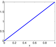
Refer to caption
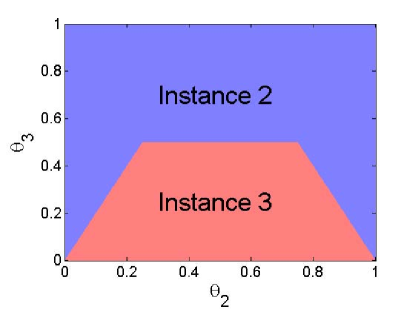
Figure 1: Decision Boundary.

Let us check a toy example with 3 instances and 5 collected labels (see Table 1). We assume that the workers are homogenous noiseless and the label aggregation is performed by the majority vote rule. Now if we only have the budget to get one more label, which instance should be chosen to label? It is obvious that we should not put the remaining budget on the first instance since we are relatively more confident on what its true label should be. Thus, the problem becomes how to choose between the second and third instances. In what follows, we shall show that there is no optimal policy under the frequentist setting. To be more explicit, the optimal policy leads to the expected accuracy which is at least as good as that of all other policies for any values of {θi}i=1nsuperscriptsubscriptsubscript𝜃𝑖𝑖1𝑛\{\theta_{i}\}_{i=1}^{n}.

Let us compute the expected improvement in accuracy in terms of the frequentist risk in Table 2. We assume that θi0.5subscript𝜃𝑖0.5\theta_{i}\neq 0.5 and if the number of 1 and 11-1 labels are the same for an instance, the accuracy is 0.5 based on a random guess. From Table 2, we should not label the first instance since the improvement is always 0. This coincides with our intuition. When max(θ20.5,0.5θ2)>0.5(1θ3)subscript𝜃20.50.5subscript𝜃20.51subscript𝜃3\max(\theta_{2}-0.5,0.5-\theta_{2})>0.5(1-\theta_{3}) or θ3>0.5subscript𝜃30.5\theta_{3}>0.5, which corresponds to the blue region in Figure 1, we should choose to label the second instance. Otherwise, we should ask the label for the third one. Since the true value of θ2subscript𝜃2\theta_{2} and θ3subscript𝜃3\theta_{3} are unknown, a optimal policy does not exist under the frequentist paradigm. Further, it will be difficult to estimate θ2subscript𝜃2\theta_{2} and θ3subscript𝜃3\theta_{3} accurately when the budget is very limited.

In contrast, in a Bayesian setting with prior distribution on each θisubscript𝜃𝑖\theta_{i}, the optimal policy is defined as the policy which leads to the highest expected accuracy under the given prior instead of for any possible values of {θi}i=1nsuperscriptsubscriptsubscript𝜃𝑖𝑖1𝑛\{\theta_{i}\}_{i=1}^{n}. Therefore, we can optimally determine the next instance to label by taking another expectation over the distribution of θisubscript𝜃𝑖\theta_{i}. In this paper, we adopt the Bayesian modeling to formulate the budget allocation problem in crowd labeling.

3 Bayesian MDP and Optimal Policy

In this section, we introduce a Bayesian MDP framework and discuss its optimal policy.

3.1 Bayesian Modeling

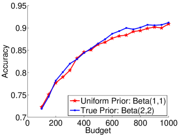
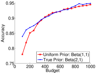
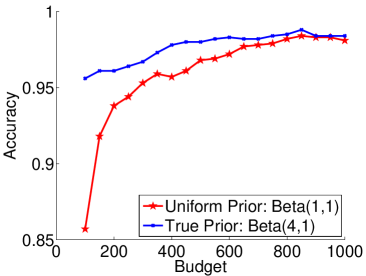
We assume that each θisubscript𝜃𝑖\theta_{i} is drawn from a known Beta prior Beta(ai0,bi0)Betasubscriptsuperscript𝑎0𝑖subscriptsuperscript𝑏0𝑖\text{Beta}(a^{0}_{i},b^{0}_{i}). Beta is a rich family of distributions in the sense that it exhibits a fairly wide variety of shapes on the domain of θisubscript𝜃𝑖\theta_{i}, i.e., the unit interval [0,1]01[0,1]. For presentation simplicity, instead of considering a full Bayesian model with hyperpriors on ai0subscriptsuperscript𝑎0𝑖a^{0}_{i} and bi0subscriptsuperscript𝑏0𝑖b^{0}_{i}, we fix ai0superscriptsubscript𝑎𝑖0a_{i}^{0} and bi0superscriptsubscript𝑏𝑖0b_{i}^{0} at the beginning. In practice, if the budget is sufficient, one can first label each instance equally many times to pre-estimate {ai0,bi0}i=1Ksuperscriptsubscriptsuperscriptsubscript𝑎𝑖0superscriptsubscript𝑏𝑖0𝑖1𝐾\{a_{i}^{0},b_{i}^{0}\}_{i=1}^{K} before the dynamic labeling procedure is invoked. Otherwise, when there is no prior knowledge, we can simply assume ai0=bi0=1superscriptsubscript𝑎𝑖0superscriptsubscript𝑏𝑖01a_{i}^{0}=b_{i}^{0}=1 so that the prior is a uniform distribution. According to our simulated experimental results in Section 8.1.2, uniform prior works reasonably well unless the data is highly skewed in terms of class distribution. Other commonly used uninformative priors such as Jeffreys prior or reference prior (Beta(1/2,1/2)Beta1212\text{Beta}(1/2,1/2)) or Haldane prior (Beta(0,0)Beta00\text{Beta}(0,0)) can also be adopted (see [31] for more on uninformative priors). Choices of prior distributions are discussed in more details in Section 4.2.

At each stage t𝑡t with Beta(ait,bit)Betasuperscriptsubscript𝑎𝑖𝑡superscriptsubscript𝑏𝑖𝑡\text{Beta}(a_{i}^{t},b_{i}^{t}) as the current posterior distribution for θisubscript𝜃𝑖\theta_{i}, we make a decision by choosing an instance it𝒜={1,,K}subscript𝑖𝑡𝒜1𝐾i_{t}\in\mathcal{A}=\{1,\ldots,K\} and acquire its label yitBernoulli(θit)similar-tosubscript𝑦subscript𝑖𝑡Bernoullisubscript𝜃subscript𝑖𝑡y_{i_{t}}\sim\text{Bernoulli}(\theta_{i_{t}}). Here 𝒜𝒜\mathcal{A} denotes the action set. By the fact that Beta is the conjugate prior of the Bernoulli, the posterior of θitsubscript𝜃subscript𝑖𝑡\theta_{i_{t}} in the stage t+1𝑡1t+1 will be updated as:

Beta(aitt+1,bitt+1)={Beta(aitt+1,bitt)ifyit=1;Beta(aitt,bitt+1)ifyit=1.Betasuperscriptsubscript𝑎subscript𝑖𝑡𝑡1superscriptsubscript𝑏subscript𝑖𝑡𝑡1casesBetasuperscriptsubscript𝑎subscript𝑖𝑡𝑡1superscriptsubscript𝑏subscript𝑖𝑡𝑡ifsubscript𝑦subscript𝑖𝑡1Betasuperscriptsubscript𝑎subscript𝑖𝑡𝑡superscriptsubscript𝑏subscript𝑖𝑡𝑡1ifsubscript𝑦subscript𝑖𝑡1\displaystyle\text{Beta}(a_{i_{t}}^{t+1},b_{i_{t}}^{t+1})=\begin{cases}\text{Beta}(a_{i_{t}}^{t}+1,b_{i_{t}}^{t})\quad&\text{if}\quad y_{i_{t}}=1;\\ \text{Beta}(a_{i_{t}}^{t},b_{i_{t}}^{t}+1)\quad&\text{if}\quad y_{i_{t}}=-1.\end{cases}

We put {ait,bit}i=1Ksuperscriptsubscriptsuperscriptsubscript𝑎𝑖𝑡superscriptsubscript𝑏𝑖𝑡𝑖1𝐾\{a_{i}^{t},b_{i}^{t}\}_{i=1}^{K} into a K×2𝐾2K\times 2 matrix Stsuperscript𝑆𝑡S^{t}, called a state matrix, and let Sit=(ait,bit)superscriptsubscript𝑆𝑖𝑡superscriptsubscript𝑎𝑖𝑡superscriptsubscript𝑏𝑖𝑡S_{i}^{t}=(a_{i}^{t},b_{i}^{t}) be the i𝑖i-th row of Stsuperscript𝑆𝑡S^{t}. The update of the state matrix can be written in a more compact form:

St+1={St+(𝐞it,𝟎)ifyit=1;St+(𝟎,𝐞it)ifyit=1,superscript𝑆𝑡1casessuperscript𝑆𝑡subscript𝐞subscript𝑖𝑡0ifsubscript𝑦subscript𝑖𝑡1superscript𝑆𝑡0subscript𝐞subscript𝑖𝑡ifsubscript𝑦subscript𝑖𝑡1S^{t+1}=\begin{cases}S^{t}+(\mathbf{e}_{i_{t}},\mathbf{0})&\text{if}\;y_{i_{t}}=1;\\ S^{t}+(\mathbf{0},\mathbf{e}_{i_{t}})&\text{if}\;y_{i_{t}}=-1,\end{cases} (2)

where 𝐞itsubscript𝐞subscript𝑖𝑡\mathbf{e}_{i_{t}} is a K×1𝐾1K\times 1 vector with 111 at the itsubscript𝑖𝑡i_{t}-th entry and 0 at all other entries. As we can see, {St}superscript𝑆𝑡\{S^{t}\} is a Markovian process because St+1superscript𝑆𝑡1S^{t+1} is completely determined by the current state Stsuperscript𝑆𝑡S^{t}, the action itsubscript𝑖𝑡i_{t} and the obtained label yitsubscript𝑦subscript𝑖𝑡y_{i_{t}}. It is easy to calculate the state transition probability Pr(yit|St,it)Prconditionalsubscript𝑦subscript𝑖𝑡superscript𝑆𝑡subscript𝑖𝑡\Pr(y_{i_{t}}|S^{t},i_{t}), which is the posterior probability that we are in the next state St+1superscript𝑆𝑡1S^{t+1} if we choose itsubscript𝑖𝑡i_{t} to be label in the current state Stsuperscript𝑆𝑡S^{t}:

Pr(yit=1|St,it)=𝔼(θit|St)=aittaitt+bittandPr(yit=1|St,it)=bittaitt+bittformulae-sequencePrsubscript𝑦subscript𝑖𝑡conditional1superscript𝑆𝑡subscript𝑖𝑡𝔼conditionalsubscript𝜃subscript𝑖𝑡superscript𝑆𝑡subscriptsuperscript𝑎𝑡subscript𝑖𝑡subscriptsuperscript𝑎𝑡subscript𝑖𝑡subscriptsuperscript𝑏𝑡subscript𝑖𝑡andPrsubscript𝑦subscript𝑖𝑡conditional1superscript𝑆𝑡subscript𝑖𝑡subscriptsuperscript𝑏𝑡subscript𝑖𝑡subscriptsuperscript𝑎𝑡subscript𝑖𝑡subscriptsuperscript𝑏𝑡subscript𝑖𝑡\displaystyle\Pr(y_{i_{t}}=1|S^{t},i_{t})=\mathbb{E}(\theta_{i_{t}}|S^{t})=\frac{a^{t}_{i_{t}}}{a^{t}_{i_{t}}+b^{t}_{i_{t}}}\quad\text{and}\quad\Pr(y_{i_{t}}=-1|S^{t},i_{t})=\frac{b^{t}_{i_{t}}}{a^{t}_{i_{t}}+b^{t}_{i_{t}}} (3)

Given this labeling process, the budget allocation policy is defined as a sequence of decisions: π=(i0,,iT1)𝜋subscript𝑖0subscript𝑖𝑇1\pi=(i_{0},\ldots,i_{T-1}). Here, we require decisions depend only upon the previous information. To make this more formal, we define a filtration {t}t=0Tsuperscriptsubscriptsubscript𝑡𝑡0𝑇\{\mathcal{F}_{t}\}_{t=0}^{T}, where tsubscript𝑡\mathcal{F}_{t} is the information collected until the stage t1𝑡1t-1. More precisely, tsubscript𝑡\mathcal{F}_{t} is the the σ𝜎\sigma-algebra generated by the sample path (i0,yi0,,it1,yit1)subscript𝑖0subscript𝑦subscript𝑖0subscript𝑖𝑡1subscript𝑦subscript𝑖𝑡1(i_{0},y_{i_{0}},\ldots,i_{t-1},y_{i_{t-1}}). We require the action itsubscript𝑖𝑡i_{t} is determined based on the historical labeling results up to the stage t1𝑡1t-1, i.e., itsubscript𝑖𝑡i_{t} is tsubscript𝑡\mathcal{F}_{t}-measurable.

3.2 Inference about the True Labels

As described in Section 2, the budget allocation process has two phases: the dynamic budget allocation phase and the label aggregation phase. Since the goal of the dynamic budget allocation in the first phase is to maximize the accuracy of aggregated labels in the second phase, we first present how to infer the true label via label aggregation in the second phase.

When the decision process terminates at the stage T𝑇T, we need to determine a positive set HTsubscript𝐻𝑇H_{T} to maximize the conditional expected accuracy conditioning on Tsubscript𝑇\mathcal{F}_{T}, which corresponds to minimizing the posterior risk:

HT=argmaxH{1,,K}𝔼(i=1K(𝟏(iH)𝟏(iH)+𝟏(iH)𝟏(iH))|T),subscript𝐻𝑇subscriptargmax𝐻1𝐾𝔼conditionalsuperscriptsubscript𝑖1𝐾1𝑖𝐻1𝑖superscript𝐻1𝑖𝐻1𝑖superscript𝐻subscript𝑇H_{T}=\mathop{\mathrm{arg\,max}{}}_{H\subset\{1,\ldots,K\}}\mathbb{E}\left(\sum_{i=1}^{K}\bigl{(}\mathbf{1}(i\in H)\cdot\mathbf{1}(i\in H^{*})+\mathbf{1}(i\not\in H)\cdot\mathbf{1}(i\not\in H^{*})\bigr{)}\Bigg{|}\mathcal{F}_{T}\right), (4)

where 𝟏()1\mathbf{1}(\cdot) is the indicator function111For example, 𝟏(iH)=11𝑖superscript𝐻1\mathbf{1}(i\in H^{*})=1 if iH𝑖superscript𝐻i\in H^{*} and 0 if iH𝑖superscript𝐻i\not\in H^{*}.. The term inside expectation in (4) is the binary labeling accuracy which can also be written as |HH|+|Hc(H)c|𝐻superscript𝐻superscript𝐻𝑐superscriptsuperscript𝐻𝑐|H\cap H^{*}|+|H^{c}\cap(H^{*})^{c}|.

We first observe that, for 0tT0𝑡𝑇0\leq t\leq T, the conditional distribution θi|tconditionalsubscript𝜃𝑖subscript𝑡\theta_{i}|\mathcal{F}_{t} is exactly the posterior distribution Beta(ait,bit)Betasuperscriptsubscript𝑎𝑖𝑡superscriptsubscript𝑏𝑖𝑡\text{Beta}(a_{i}^{t},b_{i}^{t}), which depends on the historical sampling results only through Sit=(ait,bit)superscriptsubscript𝑆𝑖𝑡superscriptsubscript𝑎𝑖𝑡superscriptsubscript𝑏𝑖𝑡S_{i}^{t}=(a_{i}^{t},b_{i}^{t}). Hence, we define

I(a,b)Pr(θ0.5|θBeta(a,b)),approaches-limit𝐼𝑎𝑏Pr𝜃conditional0.5𝜃similar-toBeta𝑎𝑏\displaystyle I(a,b)\doteq\Pr(\theta\geq 0.5|\theta\sim\mathrm{Beta}(a,b)), (5)
PitPr(iH|t)=Pr(θi0.5|t)=Pr(θi0.5|Sit)=I(ait,bit),approaches-limitsubscriptsuperscript𝑃𝑡𝑖Pr𝑖conditionalsuperscript𝐻subscript𝑡Prsubscript𝜃𝑖conditional0.5subscript𝑡Prsubscript𝜃𝑖conditional0.5superscriptsubscript𝑆𝑖𝑡𝐼superscriptsubscript𝑎𝑖𝑡superscriptsubscript𝑏𝑖𝑡\displaystyle P^{t}_{i}\doteq\Pr(i\in H^{*}|\mathcal{F}_{t})=\Pr(\theta_{i}\geq 0.5|\mathcal{F}_{t})=\Pr(\theta_{i}\geq 0.5|S_{i}^{t})=I(a_{i}^{t},b_{i}^{t}), (6)

As shown in [39], the optimal positive set HTsubscript𝐻𝑇H_{T} can be determined by the Bayes decision rule as follows.

Proposition 3.1

HT={i:Pr(iH|T)0.5}={i:PiT0.5}subscript𝐻𝑇conditional-set𝑖Pr𝑖conditionalsuperscript𝐻subscript𝑇0.5conditional-set𝑖superscriptsubscript𝑃𝑖𝑇0.5H_{T}=\{i:\Pr(i\in H^{*}|\mathcal{F}_{T})\geq 0.5\}=\{i:P_{i}^{T}\geq 0.5\} solves (4).

The proof of Proposition 3.1 is given in the appendix for completeness.

With Proposition 3.1 in place, we plug the optimal positive set HTsubscript𝐻𝑇H_{T} into the right hand side of (4) and the conditional expected accuracy given Tsubscript𝑇\mathcal{F}_{T} can be simplified as:

𝔼(i=1K(𝟏(iHT)𝟏(iH)+𝟏(iHT)𝟏(iH))|T)=i=1Kh(PiT),𝔼conditionalsuperscriptsubscript𝑖1𝐾1𝑖subscript𝐻𝑇1𝑖superscript𝐻1𝑖subscript𝐻𝑇1𝑖superscript𝐻subscript𝑇superscriptsubscript𝑖1𝐾superscriptsubscript𝑃𝑖𝑇\mathbb{E}\left(\sum_{i=1}^{K}\bigl{(}\mathbf{1}(i\in H_{T})\cdot\mathbf{1}(i\in H^{*})+\mathbf{1}(i\not\in H_{T})\cdot\mathbf{1}(i\not\in H^{*})\bigr{)}\Bigg{|}\mathcal{F}_{T}\right)=\sum_{i=1}^{K}h(P_{i}^{T}), (7)

where h(x)max(x,1x)approaches-limit𝑥𝑥1𝑥h(x)\doteq\max(x,1-x). We also note that PiTsuperscriptsubscript𝑃𝑖𝑇P_{i}^{T} provides not only the estimated label for the i𝑖i-th instance but also how confident the estimated label is correct. According to the next corollary with the proof in the appendix, we show that the optimal HTsubscript𝐻𝑇H_{T} is constructed based on a refined majority vote rule which incorporates the prior information.

Corollary 3.2

I(a,b)>0.5𝐼𝑎𝑏0.5I(a,b)>0.5 if and only if a>b𝑎𝑏a>b and I(a,b)=0.5𝐼𝑎𝑏0.5I(a,b)=0.5 if and only if a=b𝑎𝑏a=b. Therefore, HT={i:aiTbiT}subscript𝐻𝑇conditional-set𝑖subscriptsuperscript𝑎𝑇𝑖superscriptsubscript𝑏𝑖𝑇H_{T}=\{i:a^{T}_{i}\geq b_{i}^{T}\} solves (4).

By viewing ai0superscriptsubscript𝑎𝑖0a_{i}^{0} and bi0superscriptsubscript𝑏𝑖0b_{i}^{0} as pseudo-counts of 1s and 11-1s at the initial stage, the parameters aiTsuperscriptsubscript𝑎𝑖𝑇a_{i}^{T} and biTsuperscriptsubscript𝑏𝑖𝑇b_{i}^{T} are the total counts of 1s and 11-1s. The estimated positive set HT={i:aiTbiT}subscript𝐻𝑇conditional-set𝑖subscriptsuperscript𝑎𝑇𝑖superscriptsubscript𝑏𝑖𝑇H_{T}=\{i:a^{T}_{i}\geq b_{i}^{T}\} consists of instances with more (or equal) counts of 1s than that of 11-1s. When ai0=bi0superscriptsubscript𝑎𝑖0superscriptsubscript𝑏𝑖0a_{i}^{0}=b_{i}^{0}, HTsubscript𝐻𝑇H_{T} is constructed exactly according to the vanilla majority vote rule.

To find the optimal allocation policy which maximizes the expected accuracy, we need to solve the following optimization problem:

V(S0)approaches-limit𝑉superscript𝑆0absent\displaystyle V(S^{0})\doteq supπ𝔼π[𝔼(i=1K(𝟏(iHT)𝟏(iH)+𝟏(iHT)𝟏(iH))|T)]subscriptsupremum𝜋superscript𝔼𝜋delimited-[]𝔼conditionalsuperscriptsubscript𝑖1𝐾1𝑖subscript𝐻𝑇1𝑖superscript𝐻1𝑖subscript𝐻𝑇1𝑖superscript𝐻subscript𝑇\displaystyle\sup_{\pi}\mathbb{E}^{\pi}\left[\mathbb{E}\left(\sum_{i=1}^{K}\bigl{(}\mathbf{1}(i\in H_{T})\cdot\mathbf{1}(i\in H^{*})+\mathbf{1}(i\not\in H_{T})\cdot\mathbf{1}(i\not\in H^{*})\bigr{)}\Bigg{|}\mathcal{F}_{T}\right)\right]
=\displaystyle= supπ𝔼π(i=1Kh(PiT)),subscriptsupremum𝜋superscript𝔼𝜋superscriptsubscript𝑖1𝐾superscriptsubscript𝑃𝑖𝑇\displaystyle\sup_{\pi}\mathbb{E}^{\pi}\left(\sum_{i=1}^{K}h(P_{i}^{T})\right), (8)

where 𝔼πsuperscript𝔼𝜋\mathbb{E}^{\pi} represents the expectation taken over the sample paths (i0,yi0,,iT1,yiT1)subscript𝑖0subscript𝑦subscript𝑖0subscript𝑖𝑇1subscript𝑦subscript𝑖𝑇1(i_{0},y_{i_{0}},\dots,i_{T-1},y_{i_{T-1}}) generated by a policy π𝜋\pi. The second equality is due to Proposition 3.1 and V(S0)𝑉superscript𝑆0V(S^{0}) is called value function at the initial state S0superscript𝑆0S^{0}. The optimal policy πsuperscript𝜋\pi^{*} is any policy π𝜋\pi that attains the supremum in (8).

3.3 Markov Decision Process

The optimization problem in (8) is essentially a Bayesian multi-armed bandit (MAB) problem, where each instance corresponds to an arm and the decision is which instance/arm to be sampled next. However, it is different from the classical MAB problem [1, 5], which assumes that each sample of an arm yields independent and identically distributed (i.i.d.) reward according to some unknown distribution associated with that arm. Given the total budget T𝑇T, the goal is to determine a sequential allocation policy so that the collected rewards can be maximized. We contrast this problem with our problem: instead of collecting intermediate independent rewards on the fly, our objective in (8) merely involves the final “reward”, i.e., overall labeling accuracy, which is only available at the final stage when the budget runs out. Although there is no intermediate reward in our problem, we can still decompose the final expected accuracy into sum of stage-wise rewards using the technique from [39], which further leads to our MDP formulation. Since these stage-wise rewards are artificially created, they are no longer i.i.d. for each instance. We also note that the problem in [39] is an infinite-horizon one which optimizes the stopping time while our problem is finite-horizon since the decision process must be stopped at the stage T𝑇T.

Proposition 3.3

Define the stage-wise expected reward as:

R(St,it)=𝔼(i=1Kh(Pit+1)i=1Kh(Pit)|St,it)=𝔼(h(Pitt+1)h(Pitt)|St,it),𝑅superscript𝑆𝑡subscript𝑖𝑡𝔼superscriptsubscript𝑖1𝐾superscriptsubscript𝑃𝑖𝑡1conditionalsuperscriptsubscript𝑖1𝐾superscriptsubscript𝑃𝑖𝑡superscript𝑆𝑡subscript𝑖𝑡𝔼superscriptsubscript𝑃subscript𝑖𝑡𝑡1conditionalsuperscriptsubscript𝑃subscript𝑖𝑡𝑡superscript𝑆𝑡subscript𝑖𝑡R(S^{t},i_{t})=\mathbb{E}\left(\sum_{i=1}^{K}h(P_{i}^{t+1})-\sum_{i=1}^{K}h(P_{i}^{t})\big{|}S^{t},i_{t}\right)=\mathbb{E}\left(h(P_{i_{t}}^{t+1})-h(P_{i_{t}}^{t})|S^{t},i_{t}\right), (9)

then the value function (8) becomes:

V(S0)=G0(S0)+supπ𝔼π(t=0T1R(St,it)),𝑉superscript𝑆0subscript𝐺0superscript𝑆0subscriptsupremum𝜋superscript𝔼𝜋superscriptsubscript𝑡0𝑇1𝑅superscript𝑆𝑡subscript𝑖𝑡V(S^{0})=G_{0}(S^{0})+\sup_{\pi}\mathbb{E}^{\pi}\left(\sum_{t=0}^{T-1}R(S^{t},i_{t})\right), (10)

where G0(S0)=i=1Kh(Pi0)subscript𝐺0superscript𝑆0superscriptsubscript𝑖1𝐾superscriptsubscript𝑃𝑖0G_{0}(S^{0})=\sum_{i=1}^{K}h(P_{i}^{0}) and the optimal policy πsuperscript𝜋\pi^{*} is any policy π𝜋\pi that attains the supremum.

The proof of Proposition 3.3 is presented in the appendix. In fact, the stage-wise reward in (9) has a straightforward interpretation. According to (8), the term i=1Kh(Pit)superscriptsubscript𝑖1𝐾superscriptsubscript𝑃𝑖𝑡\sum_{i=1}^{K}h(P_{i}^{t}) is the expected accuracy at the t𝑡t-th stage. The stage-wise reward R(St,it)𝑅superscript𝑆𝑡subscript𝑖𝑡R(S^{t},i_{t}) takes the form of the difference between the expected accuracy at the (t+1)𝑡1(t+1)-stage and the t𝑡t-th stage, i.e., the expected gain in accuracy for collecting another label for the itsubscript𝑖𝑡i_{t}-th instance. The second equality in (9) holds simply because: only the itsubscript𝑖𝑡i_{t}-th instance receives the new label and the corresponding Pittsuperscriptsubscript𝑃subscript𝑖𝑡𝑡P_{i_{t}}^{t} changes while all other Pitsuperscriptsubscript𝑃𝑖𝑡P_{i}^{t} remain the same. Since the expected reward (9) only depends on Sitt=(aitt,bitt)superscriptsubscript𝑆subscript𝑖𝑡𝑡superscriptsubscript𝑎subscript𝑖𝑡𝑡superscriptsubscript𝑏subscript𝑖𝑡𝑡S_{i_{t}}^{t}=(a_{i_{t}}^{t},b_{i_{t}}^{t}), we write

R(St,it)=R(Sitt)=R(aitt,bitt),𝑅superscript𝑆𝑡subscript𝑖𝑡𝑅subscriptsuperscript𝑆𝑡subscript𝑖𝑡𝑅subscriptsuperscript𝑎𝑡subscript𝑖𝑡subscriptsuperscript𝑏𝑡subscript𝑖𝑡R(S^{t},i_{t})=R\left(S^{t}_{i_{t}}\right)=R\left(a^{t}_{i_{t}},b^{t}_{i_{t}}\right), (11)

and use them interchangeably. The function R(a,b)𝑅𝑎𝑏R(a,b) with two parameters a𝑎a and b𝑏b has an analytical representation as follows. For any state (a,b)𝑎𝑏(a,b) of a single instance, the reward of getting a label 1 and a label 11-1 are:

R1(a,b)subscript𝑅1𝑎𝑏\displaystyle R_{1}(a,b) =h(I(a+1,b))h(I(a,b)),absent𝐼𝑎1𝑏𝐼𝑎𝑏\displaystyle=h(I(a+1,b))-h(I(a,b)), (12)
R2(a,b)subscript𝑅2𝑎𝑏\displaystyle R_{2}(a,b) =h(I(a,b+1))h(I(a,b)).absent𝐼𝑎𝑏1𝐼𝑎𝑏\displaystyle=h(I(a,b+1))-h(I(a,b)). (13)

The expected reward takes the following form:

R(a,b)=p1R1+p2R2,𝑅𝑎𝑏subscript𝑝1subscript𝑅1subscript𝑝2subscript𝑅2R(a,b)=p_{1}R_{1}+p_{2}R_{2}, (14)

where p1=aa+bsubscript𝑝1𝑎𝑎𝑏p_{1}=\frac{a}{a+b} and p2=ba+bsubscript𝑝2𝑏𝑎𝑏p_{2}=\frac{b}{a+b} are the transition probabilities in (3).

With Proposition 3.3, the maximization problem (8) is formulated as a T𝑇T-stage Markov Decision Process (MDP) as in (10), which is associated with a tuple:

{T,{𝒮t},𝒜,Pr(yit|St,it),R(St,it)}.𝑇superscript𝒮𝑡𝒜Prconditionalsubscript𝑦subscript𝑖𝑡superscript𝑆𝑡subscript𝑖𝑡𝑅superscript𝑆𝑡subscript𝑖𝑡\{T,\{\mathcal{S}^{t}\},\mathcal{A},\Pr(y_{i_{t}}|S^{t},i_{t}),R(S^{t},i_{t})\}.

Here, the state space at the stage t𝑡t, 𝒮tsuperscript𝒮𝑡\mathcal{S}^{t}, is all possible states that can be reached at t𝑡t. Once we collect a label yitsubscript𝑦subscript𝑖𝑡y_{i_{t}}, one element in Stsuperscript𝑆𝑡S^{t} (either aittsuperscriptsubscript𝑎subscript𝑖𝑡𝑡a_{i_{t}}^{t} or bittsuperscriptsubscript𝑏subscript𝑖𝑡𝑡b_{i_{t}}^{t}) will add one. Therefore, we have

𝒮t={{ait,bit}i=1K:aitai0,bitbi0,i=1K(aitai0)+(bitbi0)=t}.superscript𝒮𝑡conditional-setsuperscriptsubscriptsuperscriptsubscript𝑎𝑖𝑡superscriptsubscript𝑏𝑖𝑡𝑖1𝐾formulae-sequencesuperscriptsubscript𝑎𝑖𝑡superscriptsubscript𝑎𝑖0formulae-sequencesuperscriptsubscript𝑏𝑖𝑡superscriptsubscript𝑏𝑖0superscriptsubscript𝑖1𝐾superscriptsubscript𝑎𝑖𝑡superscriptsubscript𝑎𝑖0superscriptsubscript𝑏𝑖𝑡superscriptsubscript𝑏𝑖0𝑡\mathcal{S}^{t}=\left\{\{a_{i}^{t},b_{i}^{t}\}_{i=1}^{K}:a_{i}^{t}\geq a_{i}^{0},b_{i}^{t}\geq b_{i}^{0},\sum_{i=1}^{K}(a_{i}^{t}-a_{i}^{0})+(b_{i}^{t}-b_{i}^{0})=t\right\}. (15)

The action space is the set of instances that could be labeled next: 𝒜={1,,K}𝒜1𝐾\mathcal{A}=\{1,\ldots,K\}. The transition probability Pr(yit|St,it)Prconditionalsubscript𝑦subscript𝑖𝑡superscript𝑆𝑡subscript𝑖𝑡\Pr(y_{i_{t}}|S^{t},i_{t}) is defined in (3) and the expected reward at each stage R(St,it)𝑅superscript𝑆𝑡subscript𝑖𝑡R(S^{t},i_{t}) is defined in (9).

  • Remark

    We can also view Proposition 3.3 as a consequence of applying the reward shaping technique [24] to the original problem (8). In fact, we can add an artificial absorbing state, named Sobssubscript𝑆𝑜𝑏𝑠S_{obs}, to the original state space (15) and assume that, when the budget allocation process finishes, the state must transit one more time to reach Sobssubscript𝑆𝑜𝑏𝑠S_{obs} regardless of which action is taken. Hence, the original problem (8) becomes a MDP that generates a zero transition reward until the state enters Sobssubscript𝑆𝑜𝑏𝑠S_{obs} where the transition reward is i=1Kh(PiT)superscriptsubscript𝑖1𝐾superscriptsubscript𝑃𝑖𝑇\sum_{i=1}^{K}h(P_{i}^{T}). Then, we define a potential-based shaping function [24] over this extended state space as Φ(St)=i=1Kh(Pit)Φsuperscript𝑆𝑡superscriptsubscript𝑖1𝐾superscriptsubscript𝑃𝑖𝑡\Phi(S^{t})=\sum_{i=1}^{K}h(P_{i}^{t}) for St𝒮tsuperscript𝑆𝑡superscript𝒮𝑡S^{t}\in\mathcal{S}^{t} and Φ(Sobs)=0Φsubscript𝑆𝑜𝑏𝑠0\Phi(S_{obs})=0. After this, (3.3) can be viewed as a new MDP whose transition reward equals that of (8) plus the shaping-reward function Φ(S)Φ(S)Φsuperscript𝑆Φ𝑆\Phi(S^{\prime})-\Phi(S) when the state transits from S𝑆S to Ssuperscript𝑆S^{\prime}. According to Theorem 1 in [24], (3.3) and (8) have the same optimal policy. This provides an alternative justification for Proposition 3.3.

3.4 Optimal Policy via DP

With the MDP in place, we can apply the dynamic programming (DP) algorithm (a.k.a. backward induction) [29] to compute the optimal policy:

  1. 1.

    Set VT1(ST1)=maxi{1,,K}R(ST1,i)subscript𝑉𝑇1superscript𝑆𝑇1subscript𝑖1𝐾𝑅superscript𝑆𝑇1𝑖V_{T-1}(S^{T-1})=\max_{i\in\{1,\ldots,K\}}R(S^{T-1},i) for all possible states ST1𝒮T1superscript𝑆𝑇1superscript𝒮𝑇1S^{T-1}\in\mathcal{S}^{T-1}. The optimal decision iT1(ST1)superscriptsubscript𝑖𝑇1superscript𝑆𝑇1i_{T-1}^{*}(S^{T-1}) is the decision i𝑖i that achieves the maximum when the state is ST1superscript𝑆𝑇1S^{T-1}.

  2. 2.

    Iterate for t=T2,,0𝑡𝑇20t=T-2,\ldots,0, compute the Vt(St)subscript𝑉𝑡superscript𝑆𝑡V_{t}(S^{t}) for all possible St𝒮tsuperscript𝑆𝑡superscript𝒮𝑡S^{t}\in\mathcal{S}^{t} using the Bellman equation:

    Vt(St)=maxi(R(St,i)+Pr(yi=1|St,i)Vt+1(St+(𝐞i,𝟎))+Pr(yi=1|St,i)Vt+1(St+(𝟎,𝐞i))),subscript𝑉𝑡superscript𝑆𝑡subscript𝑖𝑅superscript𝑆𝑡𝑖Prsubscript𝑦𝑖conditional1superscript𝑆𝑡𝑖subscript𝑉𝑡1superscript𝑆𝑡subscript𝐞𝑖0Prsubscript𝑦𝑖conditional1superscript𝑆𝑡𝑖subscript𝑉𝑡1superscript𝑆𝑡0subscript𝐞𝑖V_{t}(S^{t})=\max_{i}\Bigl{(}R(S^{t},i)+\Pr(y_{i}=1|S^{t},i)V_{t+1}\left(S^{t}+(\mathbf{e}_{i},\mathbf{0})\right)+\Pr(y_{i}=-1|S^{t},i)V_{t+1}\left(S^{t}+(\mathbf{0},\mathbf{e}_{i})\right)\Bigr{)},

    and it(St)superscriptsubscript𝑖𝑡superscript𝑆𝑡i_{t}^{*}(S^{t}) is the i𝑖i that achieves the maximum.

The optimal policy π=(i0,,iT)superscript𝜋superscriptsubscript𝑖0superscriptsubscript𝑖𝑇\pi^{*}=(i_{0}^{*},\ldots,i_{T}^{*}). For an illustration purpose, we use DP to calculate the optimal instance to be labeled next in the toy example in Section 2.1 under the uniform prior B(1,1)𝐵11B(1,1) for all θisubscript𝜃𝑖\theta_{i}. Since we assume that there is only one labeling chance remaining, which corresponds to the last stage of DP, we should choose the instance iT1(ST1)=argmaxi{1,,K}R(ST1,i)superscriptsubscript𝑖𝑇1superscript𝑆𝑇1subscriptargmax𝑖1𝐾𝑅superscript𝑆𝑇1𝑖i_{T-1}^{*}(S^{T-1})=\mathop{\mathrm{arg\,max}{}}_{i\in\{1,\ldots,K\}}R(S^{T-1},i). According to the calculation in Table 3, there is a unique optimal instance for labeling, which is the second instance.

Table 3: Calculation of the expected reward for the toy example in Table 1 according to (12), (13) and (14).
Instance i𝑖i SiT1subscriptsuperscript𝑆𝑇1𝑖S^{T-1}_{i} p1subscript𝑝1p_{1} p2subscript𝑝2p_{2} R1(SiT1)subscript𝑅1subscriptsuperscript𝑆𝑇1𝑖R_{1}(S^{T-1}_{i}) R2(SiT1)subscript𝑅2subscriptsuperscript𝑆𝑇1𝑖R_{2}(S^{T-1}_{i}) R(ST1,i)=R(SiT1)𝑅superscript𝑆𝑇1𝑖𝑅subscriptsuperscript𝑆𝑇1𝑖R(S^{T-1},i)=R(S^{T-1}_{i})
1 (3,1) 3/4343/4 1/4141/4 1/161161/16 3/16316-3/16 3/4×1/16+1/4×(3/16)=0341161431603/4\times 1/16+1/4\times(-3/16)=0
2 (2,2) 1/2121/2 1/2121/2 3/163163/16 3/163163/16 1/2×3/16+1/2×3/16=3/1612316123163161/2\times 3/16+1/2\times 3/16=3/16
3 (2,1) 2/3232/3 1/3131/3 1/8181/8 1/414-1/4 2/3×1/8+1/3×(1/4)=02318131402/3\times 1/8+1/3\times(-1/4)=0

Although DP finds the optimal policy, its computation is intractable since the size of the state space |𝒮t|superscript𝒮𝑡|\mathcal{S}^{t}| grows exponentially in t𝑡t according to (15). Therefore, we need to develop a computationally efficient approximate policy, which is the goal of the next section.

4 Approximate Policies

Since DP is computationally intractable, approximate policies are needed for large-scale applications. The simplest policy is the uniform sampling (a.k.a, pure exploration), i.e., we choose the next instance uniformly and independently at random: itUniform(1,,K)similar-tosubscript𝑖𝑡Uniform1𝐾i_{t}\sim\text{Uniform}(1,\ldots,K). However, this policy does not explore any structure of the problem.

With the decomposed reward function, our problem is essentially a finite-horizon Bayesian MAB problem. Gittins [12] showed that Gittins index policy is optimal for infinite-horizon MAB with the discounted reward. It has been applied to the infinite-horizon version of problem (10) in [39]. Since our problem is finite-horizon, Gittins index is no longer optimal while it can still provide us a good heuristic index rule. However, the computational cost of Gittins index is very high: the state-of-art-method proposed by [25] requires O(T6)𝑂superscript𝑇6O(T^{6}) time and space complexity.

A computationally more attractive policy is the knowledge gradient (KG) [13, 9]. It is essentially a single-step look-ahead policy, which greedily selects the next instance with the largest expected reward:

it=argmaxi{1,,K}(R(ait,bit)aitait+bitR1(ait,bit)+bitait+bitR2(ait,bit)).subscript𝑖𝑡subscriptargmax𝑖1𝐾approaches-limit𝑅subscriptsuperscript𝑎𝑡𝑖subscriptsuperscript𝑏𝑡𝑖superscriptsubscript𝑎𝑖𝑡superscriptsubscript𝑎𝑖𝑡superscriptsubscript𝑏𝑖𝑡subscript𝑅1superscriptsubscript𝑎𝑖𝑡superscriptsubscript𝑏𝑖𝑡superscriptsubscript𝑏𝑖𝑡superscriptsubscript𝑎𝑖𝑡superscriptsubscript𝑏𝑖𝑡subscript𝑅2superscriptsubscript𝑎𝑖𝑡superscriptsubscript𝑏𝑖𝑡i_{t}=\mathop{\mathrm{arg\,max}{}}_{i\in\{1,\ldots,K\}}\left(R(a^{t}_{i},b^{t}_{i})\doteq\frac{a_{i}^{t}}{a_{i}^{t}+b_{i}^{t}}R_{1}(a_{i}^{t},b_{i}^{t})+\frac{b_{i}^{t}}{a_{i}^{t}+b_{i}^{t}}R_{2}(a_{i}^{t},b_{i}^{t})\right). (16)

As we can see, this policy corresponds to the last stage in DP and hence KG policy is optimal if only one labeling chance is remaining.

When there is a tie, if we select the smallest index i𝑖i, the policy is referred to deterministic KG while if we randomly break the tie, the policy is referred to randomized KG. Although KG has been successfully applied to many MDP problems [28], it will fail in our problem as shown in the next proposition with the proof in the appendix.

Proposition 4.1

Assuming that ai0superscriptsubscript𝑎𝑖0a_{i}^{0} and bi0superscriptsubscript𝑏𝑖0b_{i}^{0} are positive integers and letting ={i:ai0=bi0}conditional-set𝑖superscriptsubscript𝑎𝑖0superscriptsubscript𝑏𝑖0\mathcal{E}=\{i:a_{i}^{0}=b_{i}^{0}\}, then the deterministic KG policy will acquire one label for each instance in \mathcal{E} and then consistently obtain the label for the first instance even if the budget T𝑇T goes to infinity.

According to Proposition 4.1, the deterministic KG is not a consistent policy, where the consistent policy refers to the policy that will provide correct labels for all instances (i.e., HT=Hsubscript𝐻𝑇superscript𝐻H_{T}=H^{*}) almost surely when T𝑇T goes to infinity. We note that randomized KG policy can address this problem. However, from the proof of Proposition 4.1, randomized KG behaves similarly to the uniform sampling policy in many cases and its empirical performance is undesirable according to Section 8. In the next subsection, we will propose a new approximate allocation policy based on KG which is a consistent policy with superior empirical performance.

4.1 Optimistic Knowledge Gradient

Algorithm 1 Optimistic Knowledge Gradient
  Input: Parameters of prior distributions for instances {ai0,bi0}i=1Ksuperscriptsubscriptsuperscriptsubscript𝑎𝑖0superscriptsubscript𝑏𝑖0𝑖1𝐾\{a_{i}^{0},b_{i}^{0}\}_{i=1}^{K} and the budget T𝑇T.
  for t=0,,T1𝑡0𝑇1t=0,\ldots,T-1 do
     Select the next instance itsubscript𝑖𝑡i_{t} to label according to:
it=argmaxi{1,,K}(R+(ait,bit)max(R1(ait,bit),R2(ait,bit))).subscript𝑖𝑡subscriptargmax𝑖1𝐾approaches-limitsuperscript𝑅subscriptsuperscript𝑎𝑡𝑖subscriptsuperscript𝑏𝑡𝑖subscript𝑅1subscriptsuperscript𝑎𝑡𝑖subscriptsuperscript𝑏𝑡𝑖subscript𝑅2subscriptsuperscript𝑎𝑡𝑖subscriptsuperscript𝑏𝑡𝑖\qquad i_{t}=\mathop{\mathrm{arg\,max}{}}_{i\in\{1,\ldots,K\}}\left(R^{+}(a^{t}_{i},b^{t}_{i})\doteq\max(R_{1}(a^{t}_{i},b^{t}_{i}),R_{2}(a^{t}_{i},b^{t}_{i}))\right). (17)
     Acquire the label yit{1,1}subscript𝑦subscript𝑖𝑡11y_{i_{t}}\in\{-1,1\}.
     if yit=1subscript𝑦subscript𝑖𝑡1y_{i_{t}}=1 then
        aitt+1=aitt+1,bitt+1=bittformulae-sequencesubscriptsuperscript𝑎𝑡1subscript𝑖𝑡subscriptsuperscript𝑎𝑡subscript𝑖𝑡1subscriptsuperscript𝑏𝑡1subscript𝑖𝑡subscriptsuperscript𝑏𝑡subscript𝑖𝑡a^{t+1}_{i_{t}}=a^{t}_{i_{t}}+1,b^{t+1}_{i_{t}}=b^{t}_{i_{t}}; ait+1=ait,bit+1=bitformulae-sequencesubscriptsuperscript𝑎𝑡1𝑖subscriptsuperscript𝑎𝑡𝑖subscriptsuperscript𝑏𝑡1𝑖subscriptsuperscript𝑏𝑡𝑖a^{t+1}_{i}=a^{t}_{i},b^{t+1}_{i}=b^{t}_{i} for all iit𝑖subscript𝑖𝑡i\neq i_{t}.
     else
        aitt+1=aitt,bitt+1=bitt+1formulae-sequencesubscriptsuperscript𝑎𝑡1subscript𝑖𝑡subscriptsuperscript𝑎𝑡subscript𝑖𝑡subscriptsuperscript𝑏𝑡1subscript𝑖𝑡subscriptsuperscript𝑏𝑡subscript𝑖𝑡1a^{t+1}_{i_{t}}=a^{t}_{i_{t}},b^{t+1}_{i_{t}}=b^{t}_{i_{t}}+1; ait+1=ait,bit+1=bitformulae-sequencesubscriptsuperscript𝑎𝑡1𝑖subscriptsuperscript𝑎𝑡𝑖subscriptsuperscript𝑏𝑡1𝑖subscriptsuperscript𝑏𝑡𝑖a^{t+1}_{i}=a^{t}_{i},b^{t+1}_{i}=b^{t}_{i} for all iit𝑖subscript𝑖𝑡i\neq i_{t}.
     end if
  end for
  Output: The positive set HT={i:aiTbiT}subscript𝐻𝑇conditional-set𝑖subscriptsuperscript𝑎𝑇𝑖subscriptsuperscript𝑏𝑇𝑖H_{T}=\{i:a^{T}_{i}\geq b^{T}_{i}\}.

The stage-wise reward can be viewed as a random variable with a two point distribution, i.e., with the probability p1=aa+bsubscript𝑝1𝑎𝑎𝑏p_{1}=\frac{a}{a+b} of being R1(a,b)subscript𝑅1𝑎𝑏R_{1}(a,b) and the probability p2=ba+bsubscript𝑝2𝑏𝑎𝑏p_{2}=\frac{b}{a+b} of being R2(a,b)subscript𝑅2𝑎𝑏R_{2}(a,b). The KG policy selects the instance with the largest expected reward. However, it is not consistent.

In this section, we introduce a new index policy called “optimistic knowledge gradient” (Opt-KG) policy. The Opt-KG policy assumes that decision makers are optimistic in the sense that they select the next instance based on the optimistic outcome of the reward. As a simplest version of the Opt-KG policy, for any state (ait,bit)superscriptsubscript𝑎𝑖𝑡superscriptsubscript𝑏𝑖𝑡(a_{i}^{t},b_{i}^{t}), the optimistic outcome of the reward R+(ait,bit)superscript𝑅superscriptsubscript𝑎𝑖𝑡superscriptsubscript𝑏𝑖𝑡R^{+}(a_{i}^{t},b_{i}^{t}) is defined as maximum over the reward of obtaining the label 1, R1(ait,bit)subscript𝑅1subscriptsuperscript𝑎𝑡𝑖subscriptsuperscript𝑏𝑡𝑖R_{1}(a^{t}_{i},b^{t}_{i}), and the reward of obtaining the label 11-1, R2(ait,bit)subscript𝑅2subscriptsuperscript𝑎𝑡𝑖subscriptsuperscript𝑏𝑡𝑖R_{2}(a^{t}_{i},b^{t}_{i}). Then the optimistic decision maker selects the next instance i𝑖i with the largest R+(ait,bit)superscript𝑅superscriptsubscript𝑎𝑖𝑡superscriptsubscript𝑏𝑖𝑡R^{+}(a_{i}^{t},b_{i}^{t}) as in (17) in Algorithm 1. The overall decision process using the Opt-KG policy is highlighted in Algorithm 1.

In the next theorem, we prove that Opt-KG policy is consistent.

Theorem 4.2

Assuming that ai0superscriptsubscript𝑎𝑖0a_{i}^{0} and bi0superscriptsubscript𝑏𝑖0b_{i}^{0} are positive integers, the Opt-KG is a consistent policy, i.e, as T𝑇T goes to infinity, the accuracy will be 100%percent100100\% (i.e., HT=Hsubscript𝐻𝑇superscript𝐻H_{T}=H^{*}) almost surely.

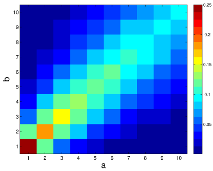
The key of proving the consistency is to show that when T𝑇T goes to infinity, each instance will be labeled infinitely many times. We prove this fact by showing that for any pair of positive integers (a,b)𝑎𝑏(a,b), R+(a,b)=max(R1(a,b),R2(a,b))>0superscript𝑅𝑎𝑏subscript𝑅1𝑎𝑏subscript𝑅2𝑎𝑏0R^{+}(a,b)=\max(R_{1}(a,b),R_{2}(a,b))>0 and R+(a,b)0superscript𝑅𝑎𝑏0R^{+}(a,b)\rightarrow 0 when a+b𝑎𝑏a+b\rightarrow\infty. As an illustration, the values of R+(a,b)superscript𝑅𝑎𝑏R^{+}(a,b) are plotted in Figure 2. Then, by strong law of large number, we obtain the consistency of the Opt-KG as stated in Theorem 4.2. The details are presented in the appendix. We have to note that asymptotic consistency is the minimum guarantee for a good policy. However, it does not necessarily guarantee the good empirical performance for the finite budget level. We will use experimental results to show the superior performance of the proposed policy.
Refer to caption
Figure 2: Illustration of R+(a,b)superscript𝑅𝑎𝑏R^{+}(a,b).

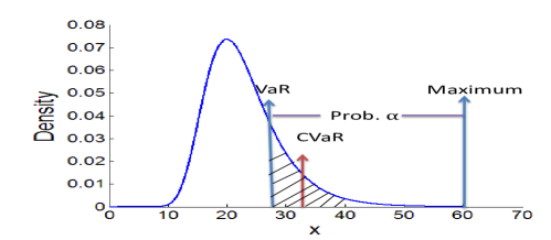
The proposed Opt-KG policy is a general framework for budget allocation in crowd labeling. We can extend the allocation policy based on the maximum over the two possible rewards (Algorithm 1) to a more general policy using the conditional value-at-risk (CVaR) [32]. We note that here, instead of adopting the CVaR as a risk measure, we apply it to the reward distribution. In particular, for a random variable X𝑋X with the support 𝒳𝒳\mathcal{X} (e.g., the random reward with the two point distribution), let α𝛼\alpha-quantile function be denoted as Qα(X)=inf{x𝒳:αFX(x)}subscript𝑄𝛼𝑋infimumconditional-set𝑥𝒳𝛼subscript𝐹𝑋𝑥Q_{\alpha}(X)=\inf\{x\in\mathcal{X}:\alpha\leq F_{X}(x)\}, where FX()subscript𝐹𝑋F_{X}(\cdot) is the CDF of X𝑋X. The value-at-risk VaRα(X)subscriptVaR𝛼𝑋\text{VaR}_{\alpha}(X) is the smallest value such that the probability that X𝑋X is less than (or equal to) it is greater than (or equal to) 1α1𝛼1-\alpha: VaRα(X)=Q1α(X)subscriptVaR𝛼𝑋subscript𝑄1𝛼𝑋\text{VaR}_{\alpha}(X)=Q_{1-\alpha}(X). The conditional value-at-risk (CVaRα(X)subscriptCVaR𝛼𝑋\text{CVaR}_{\alpha}(X)) is defined as the expected reward exceeding (or equal to) VaRα(X)subscriptVaR𝛼𝑋\text{VaR}_{\alpha}(X). An illustration of CVaR is shown in Figure 3.
Refer to caption
Figure 3: Illustration of Conditional Value-at-Risk.

For our problem, according to [32], CVaRα(X)subscriptCVaR𝛼𝑋\text{CVaR}_{\alpha}(X) can be expressed as a simple linear program:

CVaRα(X)=subscriptCVaR𝛼𝑋absent\displaystyle\text{CVaR}_{\alpha}(X)= max{q10,q20}q1R1+q2R2,subscriptformulae-sequencesubscript𝑞10subscript𝑞20subscript𝑞1subscript𝑅1subscript𝑞2subscript𝑅2\displaystyle\max_{\{q_{1}\geq 0,q_{2}\geq 0\}}q_{1}R_{1}+q_{2}R_{2},
s.t.q11αp1,q21αp2,q1+q2=1.formulae-sequences.t.subscript𝑞11𝛼subscript𝑝1formulae-sequencesubscript𝑞21𝛼subscript𝑝2subscript𝑞1subscript𝑞21\displaystyle\text{s.t.}\quad q_{1}\leq\frac{1}{\alpha}p_{1},\;q_{2}\leq\frac{1}{\alpha}p_{2},\;q_{1}+q_{2}=1.

As we can see, when α=1𝛼1\alpha=1, CVaRα(X)=p1R1+p2R2subscriptCVaR𝛼𝑋subscript𝑝1subscript𝑅1subscript𝑝2subscript𝑅2\text{CVaR}_{\alpha}(X)=p_{1}R_{1}+p_{2}R_{2}, which is the expected reward; when α0𝛼0\alpha\rightarrow 0, CVaRα(X)=max(R1,R2)subscriptCVaR𝛼𝑋subscript𝑅1subscript𝑅2\text{CVaR}_{\alpha}(X)=\max(R_{1},R_{2}), which is used as the selection criterion in (17) in Algorithm 1. In fact, a more general Opt-KG policy could be selecting the next instance with the largest CVaRα(X)subscriptCVaR𝛼𝑋\text{CVaR}_{\alpha}(X) with a tuning parameter α[0,1]𝛼01\alpha\in[0,1]. We can extend Theorem 4.2 to prove that the policy based on CVaRα(X)subscriptCVaR𝛼𝑋\text{CVaR}_{\alpha}(X) is consistent for any α<1𝛼1\alpha<1. According to our own experience, α0𝛼0\alpha\rightarrow 0 usually has a better performance in our problem especially when the budget is very limited. Therefore, for the sake of presentation simplicity, we introduce the Opt-KG using max(R1,R2)subscript𝑅1subscript𝑅2\max(R_{1},R_{2}) (i.e., α0𝛼0\alpha\rightarrow 0 in CVaRα(X)subscriptCVaR𝛼𝑋\text{CVaR}_{\alpha}(X)) as the selection criterion.

Finally, we highlight that the Opt-KG policy is computationally very efficient. For K𝐾K instances with T𝑇T units of the budget, the overall time and space complexity are O(KT)𝑂𝐾𝑇O(KT) and O(K)𝑂𝐾O(K) respectively. It is much more efficient that the Gittins index policy which requires O(T6)𝑂superscript𝑇6O(T^{6}) time and space complexity.

4.2 Discussions

It is interesting to see the connection between the idea of making the decision based on the optimistic outcome of the reward and the UCB (upper confidence bounds) policy [1] for the classical multi-armed bandit problem as described in Section 3.3. In particular, the UCB policy selects the next arm with the maximum upper confidence index, which is defined as the current average reward plus the one-sided confidence interval. As we can see, the upper confidence index can be viewed as an “optimistic” estimate of the reward. However, we note that since we are in a Bayesian setting and our stage-wise rewards are artificially created and thus not i.i.d. for each arm, the UCB policy [1] cannot be directly applied to our problem.

In fact, our Opt-KG follows a more general principle of “optimism in the face uncertainty” [35]. Essentially, the non-consistency of KG is due to its nature of pure exploitation while a consistent policy should typically utilizes exploration. One of the common techniques to handle the exploration-exploitation dilemma is to take an action based on an optimistic estimation of the rewards (see [35] and [8] ), which is the role R+(a,b)superscript𝑅𝑎𝑏R^{+}(a,b) plays in Opt-KG.

For our problem, it is also straightforward to design the “pessimistic knowledge gradient” policy which selects the next instance itsubscript𝑖𝑡i_{t} based on the pessimistic outcome of the reward, i.e.,

it=argmaxi(R(ait,bit)min(R1(ait,bit),R2(ait,bit))).subscript𝑖𝑡subscriptargmax𝑖approaches-limitsuperscript𝑅subscriptsuperscript𝑎𝑡𝑖subscriptsuperscript𝑏𝑡𝑖subscript𝑅1subscriptsuperscript𝑎𝑡𝑖subscriptsuperscript𝑏𝑡𝑖subscript𝑅2subscriptsuperscript𝑎𝑡𝑖subscriptsuperscript𝑏𝑡𝑖i_{t}=\mathop{\mathrm{arg\,max}{}}_{i}\left(R^{-}(a^{t}_{i},b^{t}_{i})\doteq\min(R_{1}(a^{t}_{i},b^{t}_{i}),R_{2}(a^{t}_{i},b^{t}_{i}))\right).

However, as shown in the next proposition with the proof in the appendix, the pessimistic KG policy is inconsistent under the uniform prior.

Proposition 4.3

When starting from the uniform prior (i.e., ai0=bi0=1superscriptsubscript𝑎𝑖0superscriptsubscript𝑏𝑖01a_{i}^{0}=b_{i}^{0}=1) for all θisubscript𝜃𝑖\theta_{i}, the pessimistic KG policy will acquire one label for each instance and then consistently acquire the label for the first instance even if the budget T𝑇T goes to infinity.

Finally, we discuss some other possible choices of prior distributions. For presentation simplicity, we only consider the Beta prior for each θisubscript𝜃𝑖\theta_{i} with the fixed parameters ai0superscriptsubscript𝑎𝑖0a_{i}^{0} and bi0superscriptsubscript𝑏𝑖0b_{i}^{0}. In practice, more complicated priors can be easily incorporated into our framework. For example, in instead of using only one Beta prior, one can adopt a mixture of Beta distributions as the prior and the posterior will also follow a mixture of Beta distributions, which allows an easy inference about the posterior. As we show in the experiments (see Section 8.1.2), the uniform prior does not work well when the data is highly skewed in terms of class distribution. To address this problem, one possible choice is to adopt the prior p(θ)=w1Beta(c,1)+w2Beta(1,1)+w3Beta(1,c)𝑝𝜃subscript𝑤1Beta𝑐1subscript𝑤2Beta11subscript𝑤3Beta1𝑐p(\theta)=w_{1}\text{Beta}(c,1)+w_{2}\text{Beta}(1,1)+w_{3}\text{Beta}(1,c) where w1,w2subscript𝑤1subscript𝑤2w_{1},w_{2} and w3subscript𝑤3w_{3} are the weights and c𝑐c is a constant larger than 1 (e.g., c=5𝑐5c=5). In such a prior, B(c,1)𝐵𝑐1B(c,1) corresponds to the data with more positive labels while B(1,c)𝐵1𝑐B(1,c) to the data with more negative labels. In addition to the mixture Beta prior, one can adopt the hierarchical Bayesian approach which puts hyper-priors on the parameters in the Beta priors. The inference can be performed using empirical Bayes approach [11, 31]. In particular, one can periodically re-calculate the MAP estimate of the hyper-parameters based on the available data and update the model, but otherwise proceed with the given hyper-parameters. For common choices of hyper-priors of Beta, please refer to Section 5.3 in [11]. These approaches can also be applied to model the workers’ reliability as we introduced in the next Section. For example, one can use a mixture of Beta distributions as the prior for the workers’ reliability, where Beta(c,1)Beta𝑐1\text{Beta}(c,1) corresponds to reliable workers, Beta(1,1)Beta11\text{Beta}(1,1) to random workers and Beta(1,c)Beta1𝑐\text{Beta}(1,c) to malicious or poorly informed workers.

5 Incorporate Reliability of Heterogeneous Workers

In push crowdsourcing marketplaces, it is important to model workers’ reliability so that the decision maker could assign more instances to reliable workers. Assuming that there are M𝑀M workers in a push marketplace, we can capture the reliability of the j𝑗j-th worker by introducing an extra parameter ρj[0,1]subscript𝜌𝑗01\rho_{j}\in[0,1] as in [6, 30, 19], which is defined as the probability of getting the same label as the one from a random fully reliable worker. Recall that the soft-label θisubscript𝜃𝑖\theta_{i} is the i𝑖i-th instance’s probability of being labeled as positive by a fully reliable worker and let zijsubscript𝑧𝑖𝑗z_{ij} be the label provided by the j𝑗j-th worker for the i𝑖i-th instance. We model the distribution of zijsubscript𝑧𝑖𝑗z_{ij} for given θisubscript𝜃𝑖\theta_{i} and ρjsubscript𝜌𝑗\rho_{j} using the one-coin model [6, 19]222We can further extend it to a more complex two-coin model [6, 30] by introducing a pair of parameters (ρj1,ρj2)subscript𝜌𝑗1subscript𝜌𝑗2(\rho_{j1},\rho_{j2}) to model the j𝑗j-th worker’s reliability. In particular, ρj1subscript𝜌𝑗1\rho_{j1} and ρj2subscript𝜌𝑗2\rho_{j2} are the probabilities of getting the positive and negative labels when a fully reliable worker provides the same label.:

Pr(zij=1|θi,ρj)Prsubscript𝑧𝑖𝑗conditional1subscript𝜃𝑖subscript𝜌𝑗\displaystyle\Pr(z_{ij}=1|\theta_{i},\rho_{j}) =Pr(zij=1|yi=1,ρj)Pr(yi=1|θi)+Pr(zij=1|yi=1,ρj)Pr(yi=1|θi)absentPrsubscript𝑧𝑖𝑗conditional1subscript𝑦𝑖1subscript𝜌𝑗Prsubscript𝑦𝑖conditional1subscript𝜃𝑖Prsubscript𝑧𝑖𝑗conditional1subscript𝑦𝑖1subscript𝜌𝑗Prsubscript𝑦𝑖conditional1subscript𝜃𝑖\displaystyle=\Pr(z_{ij}=1|y_{i}=1,\rho_{j})\Pr(y_{i}=1|\theta_{i})+\Pr(z_{ij}=1|y_{i}=-1,\rho_{j})\Pr(y_{i}=-1|\theta_{i})
=ρjθi+(1ρj)(1θi);absentsubscript𝜌𝑗subscript𝜃𝑖1subscript𝜌𝑗1subscript𝜃𝑖\displaystyle=\rho_{j}\theta_{i}+(1-\rho_{j})(1-\theta_{i}); (18)
Pr(zij=1|θi,ρj)Prsubscript𝑧𝑖𝑗conditional1subscript𝜃𝑖subscript𝜌𝑗\displaystyle\Pr(z_{ij}=-1|\theta_{i},\rho_{j}) =Pr(zij=1|yi=1,ρj)Pr(yi=1|θi)+Pr(zij=1|yi=1,ρj)Pr(yi=1|θi)absentPrsubscript𝑧𝑖𝑗conditional1subscript𝑦𝑖1subscript𝜌𝑗Prsubscript𝑦𝑖conditional1subscript𝜃𝑖Prsubscript𝑧𝑖𝑗conditional1subscript𝑦𝑖1subscript𝜌𝑗Prsubscript𝑦𝑖conditional1subscript𝜃𝑖\displaystyle=\Pr(z_{ij}=-1|y_{i}=-1,\rho_{j})\Pr(y_{i}=-1|\theta_{i})+\Pr(z_{ij}=-1|y_{i}=1,\rho_{j})\Pr(y_{i}=1|\theta_{i})
=ρj(1θi)+(1ρj)θi,absentsubscript𝜌𝑗1subscript𝜃𝑖1subscript𝜌𝑗subscript𝜃𝑖\displaystyle=\rho_{j}(1-\theta_{i})+(1-\rho_{j})\theta_{i}, (19)

where yisubscript𝑦𝑖y_{i} denotes the label provided a random fully reliable worker for the i𝑖i-th instance. Here we make the following implicit assumption:

Assumption 5.1

We assume that different workers make independent judgements and, for each single worker, the labels provided by him/her to different instances are also independent.

As the parameter ρjsubscript𝜌𝑗\rho_{j} increases from 00 to 111, the j𝑗j-th worker’s reliability also increases in the sense that Pr(zij=1|θi,ρj)Prsubscript𝑧𝑖𝑗conditional1subscript𝜃𝑖subscript𝜌𝑗\Pr(z_{ij}=1|\theta_{i},\rho_{j}) gets more and more close to θisubscript𝜃𝑖\theta_{i}, which is the probability of getting a positive label from a random fully reliable worker. Different types of workers can be easily characterized by ρjsubscript𝜌𝑗\rho_{j}. When all ρj=1subscript𝜌𝑗1\rho_{j}=1, it recovers the previous model with fully reliable workers since Pr(zij=1|θi,ρj)=θiPrsubscript𝑧𝑖𝑗conditional1subscript𝜃𝑖subscript𝜌𝑗subscript𝜃𝑖\Pr(z_{ij}=1|\theta_{i},\rho_{j})=\theta_{i}, i.e, each worker provides the label only according to the underlying soft-label of the instance. When ρj=0.5subscript𝜌𝑗0.5\rho_{j}=0.5, we have Pr(zij=1|θi,ρj)=Pr(zij=1|θi,ρj)=0.5Prsubscript𝑧𝑖𝑗conditional1subscript𝜃𝑖subscript𝜌𝑗Prsubscript𝑧𝑖𝑗conditional1subscript𝜃𝑖subscript𝜌𝑗0.5\Pr(z_{ij}=1|\theta_{i},\rho_{j})=\Pr(z_{ij}=-1|\theta_{i},\rho_{j})=0.5, which indicates that the j𝑗j-th worker is a spammer, who randomly submits positive or negative labels. When ρj=0subscript𝜌𝑗0\rho_{j}=0, it indicates that the j𝑗j-th worker is poorly informed or misunderstands the instruction such that he/she always assigns wrong labels.

We assume that instances’ soft-label {θi}i=1Ksuperscriptsubscriptsubscript𝜃𝑖𝑖1𝐾\{\theta_{i}\}_{i=1}^{K} and workers’ reliability {ρj}j=1Msuperscriptsubscriptsubscript𝜌𝑗𝑗1𝑀\{\rho_{j}\}_{j=1}^{M} are drawn from known Beta prior distributions: θiBeta(ai0,bi0)similar-tosubscript𝜃𝑖Betasuperscriptsubscript𝑎𝑖0superscriptsubscript𝑏𝑖0\theta_{i}\sim\text{Beta}(a_{i}^{0},b_{i}^{0}) and ρjBeta(cj0,dj0)similar-tosubscript𝜌𝑗Betasuperscriptsubscript𝑐𝑗0superscriptsubscript𝑑𝑗0\rho_{j}\sim\text{Beta}(c_{j}^{0},d_{j}^{0}). At each stage, we need to make the decision on both the next instance i𝑖i to be labeled and the next worker j𝑗j to label the instance i𝑖i (we omit t𝑡t in i,j𝑖𝑗i,j here for notational simplicity). In other words, the action space 𝒜={(i,j):(i,j){1,,K}×{1,,M}}𝒜conditional-set𝑖𝑗𝑖𝑗1𝐾1𝑀\mathcal{A}=\{(i,j):(i,j)\in\{1,\ldots,K\}\times\{1,\ldots,M\}\}. Once the decision is made, the distribution of the outcome zijsubscript𝑧𝑖𝑗z_{ij} is given by (18) and (19). Given the prior distributions and likelihood functions in (18) and (19), the Bayesian Markov Decision process can be formally defined as in Section 3. Similar to the homogeneous worker setting, the optimal inferred positive set HTsubscript𝐻𝑇H_{T} takes the form of HT={i:PiT0.5}subscript𝐻𝑇conditional-set𝑖superscriptsubscript𝑃𝑖𝑇0.5H_{T}=\{i:P_{i}^{T}\geq 0.5\} as in Proposition 3.1 with Pit=Pr(iH|t)=Pr(θi0.5|t)superscriptsubscript𝑃𝑖𝑡Pr𝑖conditionalsuperscript𝐻subscript𝑡Prsubscript𝜃𝑖conditional0.5subscript𝑡P_{i}^{t}=\Pr(i\in H^{*}|\mathcal{F}_{t})=\Pr\left(\theta_{i}\geq 0.5|\mathcal{F}_{t}\right). The value function V(S0)𝑉superscript𝑆0V(S^{0}) still takes the form of (8), which can be further decomposed into the sum of stage-wise rewards in (9) using Proposition 3.3. Unfortunately, in the heterogenous worker setting, the posterior distributions of θisubscript𝜃𝑖\theta_{i} and ρjsubscript𝜌𝑗\rho_{j} are highly correlated with a sophisticated joint distribution, which makes the computation of stage-wise rewards in (9) much more challenging. In particular, given the prior θiBeta(ai0,bi0)similar-tosubscript𝜃𝑖Betasuperscriptsubscript𝑎𝑖0superscriptsubscript𝑏𝑖0\theta_{i}\sim\text{Beta}(a_{i}^{0},b_{i}^{0}) and ρjBeta(cj0,dj0)similar-tosubscript𝜌𝑗Betasuperscriptsubscript𝑐𝑗0superscriptsubscript𝑑𝑗0\rho_{j}\sim\text{Beta}(c_{j}^{0},d_{j}^{0}), the posterior distribution of θisubscript𝜃𝑖\theta_{i} and ρjsubscript𝜌𝑗\rho_{j} given the label zij=z{1,1}subscript𝑧𝑖𝑗𝑧11z_{ij}=z\in\{-1,1\} takes the following form:

p(θi,ρj|zij=z)=Pr(zij=z|θi,ρj)Beta(ai0,bi0)Beta(cj0,dj0)Pr(zij=z),𝑝subscript𝜃𝑖conditionalsubscript𝜌𝑗subscript𝑧𝑖𝑗𝑧Prsubscript𝑧𝑖𝑗conditional𝑧subscript𝜃𝑖subscript𝜌𝑗Betasuperscriptsubscript𝑎𝑖0superscriptsubscript𝑏𝑖0Betasuperscriptsubscript𝑐𝑗0superscriptsubscript𝑑𝑗0Prsubscript𝑧𝑖𝑗𝑧\displaystyle p(\theta_{i},\rho_{j}|z_{ij}=z)=\frac{\Pr(z_{ij}=z|\theta_{i},\rho_{j})\text{Beta}(a_{i}^{0},b_{i}^{0})\text{Beta}(c_{j}^{0},d_{j}^{0})}{\Pr(z_{ij}=z)}, (20)

where Pr(zij=z|θi,ρj)Prsubscript𝑧𝑖𝑗conditional𝑧subscript𝜃𝑖subscript𝜌𝑗\Pr(z_{ij}=z|\theta_{i},\rho_{j}) is the likelihood function defined in (18) and (19) and

Pr(zij=1)Prsubscript𝑧𝑖𝑗1\displaystyle\Pr(z_{ij}=1) =𝔼(Pr(zij=1|θi,ρj))=𝔼(θi)𝔼(ρj)+(1𝔼(θi))(1𝔼(ρj))absent𝔼Prsubscript𝑧𝑖𝑗conditional1subscript𝜃𝑖subscript𝜌𝑗𝔼subscript𝜃𝑖𝔼subscript𝜌𝑗1𝔼subscript𝜃𝑖1𝔼subscript𝜌𝑗\displaystyle=\mathbb{E}(\Pr(z_{ij}=1|\theta_{i},\rho_{j}))=\mathbb{E}(\theta_{i})\mathbb{E}(\rho_{j})+(1-\mathbb{E}(\theta_{i}))(1-\mathbb{E}(\rho_{j}))
=ai0ai0+bi0cj0cj0+dj0+bi0ai0+bi0dj0cj0+dj0.absentsuperscriptsubscript𝑎𝑖0superscriptsubscript𝑎𝑖0superscriptsubscript𝑏𝑖0superscriptsubscript𝑐𝑗0superscriptsubscript𝑐𝑗0superscriptsubscript𝑑𝑗0superscriptsubscript𝑏𝑖0superscriptsubscript𝑎𝑖0superscriptsubscript𝑏𝑖0superscriptsubscript𝑑𝑗0superscriptsubscript𝑐𝑗0superscriptsubscript𝑑𝑗0\displaystyle=\frac{a_{i}^{0}}{a_{i}^{0}+b_{i}^{0}}\frac{c_{j}^{0}}{c_{j}^{0}+d_{j}^{0}}+\frac{b_{i}^{0}}{a_{i}^{0}+b_{i}^{0}}\frac{d_{j}^{0}}{c_{j}^{0}+d_{j}^{0}}.

As we can see, the posterior distribution p(θi,ρj|zij=z)𝑝subscript𝜃𝑖conditionalsubscript𝜌𝑗subscript𝑧𝑖𝑗𝑧p(\theta_{i},\rho_{j}|z_{ij}=z) no longer takes the form of the product of the distributions of θisubscript𝜃𝑖\theta_{i} and ρjsubscript𝜌𝑗\rho_{j} and the marginal posterior of θisubscript𝜃𝑖\theta_{i} is no longer a Beta distribution. As a result, Pitsuperscriptsubscript𝑃𝑖𝑡P_{i}^{t} does not have a simple representation as in (5), which makes the computation of the reward function much more difficult as the number of stages increases. Therefore, to apply our Opt-KG policy to large-scale applications, we need to use some approximate posterior inference techniques.

Algorithm 2 Optimistic Knowledge Gradient for Heterogeneous Workers
  Input: Parameters of prior distributions for instances {ai0,bi0}i=1Ksuperscriptsubscriptsuperscriptsubscript𝑎𝑖0superscriptsubscript𝑏𝑖0𝑖1𝐾\{a_{i}^{0},b_{i}^{0}\}_{i=1}^{K} and for workers {cj0,dj0}j=1Msuperscriptsubscriptsuperscriptsubscript𝑐𝑗0superscriptsubscript𝑑𝑗0𝑗1𝑀\{c_{j}^{0},d_{j}^{0}\}_{j=1}^{M}. The total budget T𝑇T.
  for t=0,,T1𝑡0𝑇1t=0,\ldots,T-1 do
     1. Select the next instance itsubscript𝑖𝑡i_{t} to label and the next worker jtsubscript𝑗𝑡j_{t} to label itsubscript𝑖𝑡i_{t} according to:
(it,jt)=argmax(i,j){1,,K}×{1,,M}(R+(ait,bit,cjt,djt)max(R1(ait,bit,cjt,djt),R2(ait,bit,cjt,djt))).subscript𝑖𝑡subscript𝑗𝑡subscriptargmax𝑖𝑗1𝐾1𝑀approaches-limitsuperscript𝑅subscriptsuperscript𝑎𝑡𝑖subscriptsuperscript𝑏𝑡𝑖subscriptsuperscript𝑐𝑡𝑗subscriptsuperscript𝑑𝑡𝑗subscript𝑅1subscriptsuperscript𝑎𝑡𝑖subscriptsuperscript𝑏𝑡𝑖subscriptsuperscript𝑐𝑡𝑗subscriptsuperscript𝑑𝑡𝑗subscript𝑅2subscriptsuperscript𝑎𝑡𝑖subscriptsuperscript𝑏𝑡𝑖subscriptsuperscript𝑐𝑡𝑗subscriptsuperscript𝑑𝑡𝑗(i_{t},j_{t})=\mathop{\mathrm{arg\,max}{}}_{(i,j)\in\{1,\ldots,K\}\times\{1,\ldots,M\}}\left(R^{+}(a^{t}_{i},b^{t}_{i},c^{t}_{j},d^{t}_{j})\doteq\max(R_{1}(a^{t}_{i},b^{t}_{i},c^{t}_{j},d^{t}_{j}),R_{2}(a^{t}_{i},b^{t}_{i},c^{t}_{j},d^{t}_{j}))\right). (21)
     2. Acquire the label zitjt{1,1}subscript𝑧subscript𝑖𝑡subscript𝑗𝑡11z_{i_{t}j_{t}}\in\{-1,1\} of the i𝑖i-th instance from the j𝑗j-th worker.
     3. Update the posterior by setting:
aitt+1=a~itt(zitjt)bitt+1=b~itt(zitjt)cjtt+1=c~jtt(zitjt)djtt+1=d~jtt(zitjt),formulae-sequencesubscriptsuperscript𝑎𝑡1subscript𝑖𝑡subscriptsuperscript~𝑎𝑡subscript𝑖𝑡subscript𝑧subscript𝑖𝑡subscript𝑗𝑡formulae-sequencesubscriptsuperscript𝑏𝑡1subscript𝑖𝑡subscriptsuperscript~𝑏𝑡subscript𝑖𝑡subscript𝑧subscript𝑖𝑡subscript𝑗𝑡formulae-sequencesubscriptsuperscript𝑐𝑡1subscript𝑗𝑡subscriptsuperscript~𝑐𝑡subscript𝑗𝑡subscript𝑧subscript𝑖𝑡subscript𝑗𝑡subscriptsuperscript𝑑𝑡1subscript𝑗𝑡subscriptsuperscript~𝑑𝑡subscript𝑗𝑡subscript𝑧subscript𝑖𝑡subscript𝑗𝑡\displaystyle a^{t+1}_{i_{t}}=\tilde{a}^{t}_{i_{t}}(z_{i_{t}j_{t}})\qquad b^{t+1}_{i_{t}}=\tilde{b}^{t}_{i_{t}}(z_{i_{t}j_{t}})\qquad c^{t+1}_{j_{t}}=\tilde{c}^{t}_{j_{t}}(z_{i_{t}j_{t}})\qquad d^{t+1}_{j_{t}}=\tilde{d}^{t}_{j_{t}}(z_{i_{t}j_{t}}),
and all parameters for iit𝑖subscript𝑖𝑡i\neq i_{t} and jjt𝑗subscript𝑗𝑡j\neq j_{t} remain the same.
  end for
  Output: The positive set HT={i:aiTbiT}subscript𝐻𝑇conditional-set𝑖subscriptsuperscript𝑎𝑇𝑖subscriptsuperscript𝑏𝑇𝑖H_{T}=\{i:a^{T}_{i}\geq b^{T}_{i}\}.

When applying Opt-KG, we need to perform 2KMT2𝐾𝑀𝑇2\cdot K\cdot M\cdot T inferences of the posterior distribution in total. Each approximate inference should be computed very efficiently, hopefully in a closed-form. For large-scale problems, most traditional approximate inference techniques such as Markov Chain Monte Carlo (MCMC) or variational Bayesian methods (e.g., [3, 27]) may lead to higher computational cost since each inference is an iterative procedure. To address the computational challenge, we apply the variational approximation with the moment matching technique so that each inference of the approximate posterior can be computed in a closed-form. In fact, any highly efficient approximate inference can be utilized to compute the reward function. Since the main focus of the paper is on the MDP model and Opt-KG policy, we omit the discussion for other possible approximate inference techniques. In particular, we first adopt the variational approximation by assuming the conditional independence of θisubscript𝜃𝑖\theta_{i} and ρjsubscript𝜌𝑗\rho_{j}:

p(θi,ρj|zij=z)p(θi|zij=z)p(ρj|zij=z)𝑝subscript𝜃𝑖conditionalsubscript𝜌𝑗subscript𝑧𝑖𝑗𝑧𝑝conditionalsubscript𝜃𝑖subscript𝑧𝑖𝑗𝑧𝑝conditionalsubscript𝜌𝑗subscript𝑧𝑖𝑗𝑧p(\theta_{i},\rho_{j}|z_{ij}=z)\approx p(\theta_{i}|z_{ij}=z)p(\rho_{j}|z_{ij}=z)

We further approximate p(θi|zij=z)𝑝conditionalsubscript𝜃𝑖subscript𝑧𝑖𝑗𝑧p(\theta_{i}|z_{ij}=z) and p(ρj|zij=z)𝑝conditionalsubscript𝜌𝑗subscript𝑧𝑖𝑗𝑧p(\rho_{j}|z_{ij}=z) by two Beta distributions:

p(θi|zij=z)Beta(a~i(z),b~i(z));p(ρj|zij=z)Beta(c~j(z),d~j(z)),formulae-sequence𝑝conditionalsubscript𝜃𝑖subscript𝑧𝑖𝑗𝑧Betasubscript~𝑎𝑖𝑧subscript~𝑏𝑖𝑧𝑝conditionalsubscript𝜌𝑗subscript𝑧𝑖𝑗𝑧Betasubscript~𝑐𝑗𝑧subscript~𝑑𝑗𝑧p(\theta_{i}|z_{ij}=z)\approx\text{Beta}(\tilde{a}_{i}(z),\tilde{b}_{i}(z));\qquad p(\rho_{j}|z_{ij}=z)\approx\text{Beta}(\tilde{c}_{j}(z),\tilde{d}_{j}(z)),

where the parameters a~i(z)subscript~𝑎𝑖𝑧\tilde{a}_{i}(z), b~i(z)subscript~𝑏𝑖𝑧\tilde{b}_{i}(z), c~j(z)subscript~𝑐𝑗𝑧\tilde{c}_{j}(z), d~j(z)subscript~𝑑𝑗𝑧\tilde{d}_{j}(z) are computed using moment matching with the analytical form presented in the appendix. After this approximation, the new posterior distributions of θisubscript𝜃𝑖\theta_{i} and ρjsubscript𝜌𝑗\rho_{j} still have the same structure as their prior distribution, i.e., the product of two Beta distributions, which allows a repeatable use of this approximation every time when a new label is collected. Moreover, due to the Beta distribution approximation of p(θi|zij=z)𝑝conditionalsubscript𝜃𝑖subscript𝑧𝑖𝑗𝑧p(\theta_{i}|z_{ij}=z), the reward function takes a similar form as in the previous setting. In particular, assuming at a certain stage, θisubscript𝜃𝑖\theta_{i} has the posterior distribution Beta(ai,bi)Betasubscript𝑎𝑖subscript𝑏𝑖\text{Beta}(a_{i},b_{i}) and ρjsubscript𝜌𝑗\rho_{j} has the posterior distribution Beta(cj,dj)Betasubscript𝑐𝑗subscript𝑑𝑗\text{Beta}(c_{j},d_{j}). The reward of getting positive and negative labels for the i𝑖i-th instance from the j𝑗j-th worker are presented in (22) and (23):

R1(ai,bi,cj,dj)subscript𝑅1subscript𝑎𝑖subscript𝑏𝑖subscript𝑐𝑗subscript𝑑𝑗\displaystyle R_{1}(a_{i},b_{i},c_{j},d_{j}) =h(I(a~i(z=1),b~i(z=1)))h(I(ai,bi)),absent𝐼subscript~𝑎𝑖𝑧1subscript~𝑏𝑖𝑧1𝐼subscript𝑎𝑖subscript𝑏𝑖\displaystyle=h(I(\tilde{a}_{i}(z=1),\tilde{b}_{i}(z=1)))-h(I(a_{i},b_{i})), (22)
R2(ai,bi,cj,dj)subscript𝑅2subscript𝑎𝑖subscript𝑏𝑖subscript𝑐𝑗subscript𝑑𝑗\displaystyle R_{2}(a_{i},b_{i},c_{j},d_{j}) =h(I(a~i(z=1),b~i(z=1)))h(I(ai,bi)),absent𝐼subscript~𝑎𝑖𝑧1subscript~𝑏𝑖𝑧1𝐼subscript𝑎𝑖subscript𝑏𝑖\displaystyle=h(I(\tilde{a}_{i}(z=-1),\tilde{b}_{i}(z=-1)))-h(I(a_{i},b_{i})), (23)

With the reward in place, we present Opt-KG for budget allocation in the heterogeneous worker setting in Algorithm 2. We also note that due to the variational approximation of the posterior, establishing the consistency results of Opt-KG becomes very challenging in the heterogeneous worker setting.

6 Extensions

Our MDP formulation is a general framework to address many complex settings of dynamic budget allocation problems in crowd labeling. In this section, we briefly discuss two important extensions, where for both extensions, Opt-KG can be directly applied as an approximate policy. We note that for the sake of presentation simplicity, we only present these extensions in the noiseless homogeneous worker setting. Further extensions to the heterogeneous setting are rather straightforward using the technique from Section 5.

6.1 Utilizing Contextual Information

When the contextual information is available for instances, we could easily extend our model to incorporate such an important information. In particular, let the contextual information for the i𝑖i-th instance be represented by a p𝑝p-dimensional feature vector 𝐱ipsubscript𝐱𝑖superscript𝑝\mathbf{x}_{i}\in\mathbb{R}^{p}. We could utilize the feature information by assuming a logistic model for θisubscript𝜃𝑖\theta_{i}:

θiexp{𝐰,𝐱i}1+exp{𝐰,𝐱i},approaches-limitsubscript𝜃𝑖𝐰subscript𝐱𝑖1𝐰subscript𝐱𝑖\displaystyle\theta_{i}\doteq\frac{\exp\{\langle\mathbf{w},\mathbf{x}_{i}\rangle\}}{1+\exp\{\langle\mathbf{w},\mathbf{x}_{i}\rangle\}},

where 𝐰𝐰\mathbf{w} is assumed to be drawn from a Gaussian prior N(𝝁0,𝚺0)𝑁subscript𝝁0subscript𝚺0N(\bm{\mu}_{0},\bm{\Sigma}_{0}). At the t𝑡t-th stage with the current state (𝝁t,𝚺t)subscript𝝁𝑡subscript𝚺𝑡(\bm{\mu}_{t},\bm{\Sigma}_{t}), the decision maker determines the instance itsubscript𝑖𝑡i_{t} and acquire its label yit{1,1}subscript𝑦subscript𝑖𝑡11y_{i_{t}}\in\{-1,1\}. Then we update the posterior 𝝁t+1subscript𝝁𝑡1\bm{\mu}_{t+1} and 𝚺t+1subscript𝚺𝑡1\bm{\Sigma}_{t+1} using the Laplace method as in Bayesian logistic regression [4]. Variational methods can be applied to further accelerate the posterior update [16] . The details are provided in the appendix.

6.2 Multi-Class Categorization

Our MDP formulation can also be extended to deal with multi-class categorization problems, where each instance is a multiple choice question with several possible options (i.e., classes). More formally, in a multi-class setting with C𝐶C different classes, we assume that the i𝑖i-th instance is associated with a probability vector 𝜽i=(θi1,θiC)subscript𝜽𝑖subscript𝜃𝑖1subscript𝜃𝑖𝐶\bm{\theta}_{i}=(\theta_{i1},\ldots\theta_{iC}), where θicsubscript𝜃𝑖𝑐\theta_{ic} is the probability that the i𝑖i-th instance will be labeled as the class c𝑐c by a random fully reliable worker and i=1Cθic=1superscriptsubscript𝑖1𝐶subscript𝜃𝑖𝑐1\sum_{i=1}^{C}\theta_{ic}=1. We assume that 𝜽isubscript𝜽𝑖\bm{\theta}_{i} has a Dirichlet prior 𝜽iDir(𝜶i0)similar-tosubscript𝜽𝑖Dirsuperscriptsubscript𝜶𝑖0\bm{\theta}_{i}\sim\text{Dir}(\bm{\alpha}_{i}^{0}) and the initial state S0superscript𝑆0S^{0} is a K×C𝐾𝐶K\times C matrix with 𝜶i0superscriptsubscript𝜶𝑖0\bm{\alpha}_{i}^{0} as its i𝑖i-th row. At each stage t𝑡t with the current state Stsuperscript𝑆𝑡S^{t}, we determine the next instance itsubscript𝑖𝑡i_{t} to be labeled and collect its label yit{1,,C}subscript𝑦subscript𝑖𝑡1𝐶y_{i_{t}}\in\{1,\ldots,C\}, which follows the categorical distribution: p(yit)=c=1CθitcI(yit=c)𝑝subscript𝑦subscript𝑖𝑡superscriptsubscriptproduct𝑐1𝐶superscriptsubscript𝜃subscript𝑖𝑡𝑐𝐼subscript𝑦subscript𝑖𝑡𝑐p(y_{i_{t}})=\prod_{c=1}^{C}\theta_{i_{t}c}^{I(y_{i_{t}}=c)}. Since the Dirichlet is the conjugate prior of the categorical distribution, the next state induced by the posterior distribution is: Sitt+1=Sitt+𝜹yitsubscriptsuperscript𝑆𝑡1subscript𝑖𝑡subscriptsuperscript𝑆𝑡subscript𝑖𝑡subscript𝜹subscript𝑦subscript𝑖𝑡S^{t+1}_{i_{t}}=S^{t}_{i_{t}}+\bm{\delta}_{y_{i_{t}}} and Sit+1=Sitsubscriptsuperscript𝑆𝑡1𝑖subscriptsuperscript𝑆𝑡𝑖S^{t+1}_{i}=S^{t}_{i} for all iit𝑖subscript𝑖𝑡i\neq i_{t}. Here 𝜹csubscript𝜹𝑐\bm{\delta}_{c} is a row vector with one at the c𝑐c-th entry and zeros at all other entries. The transition probability is:

Pr(yit=c|St,it)=𝔼(θitc|St)=αitctc=1Cαitct.Prsubscript𝑦subscript𝑖𝑡conditional𝑐superscript𝑆𝑡subscript𝑖𝑡𝔼conditionalsubscript𝜃subscript𝑖𝑡𝑐superscript𝑆𝑡subscriptsuperscript𝛼𝑡subscript𝑖𝑡𝑐superscriptsubscript𝑐1𝐶subscriptsuperscript𝛼𝑡subscript𝑖𝑡𝑐\Pr(y_{i_{t}}=c|S^{t},i_{t})=\mathbb{E}(\theta_{i_{t}c}|S^{t})=\frac{\alpha^{t}_{i_{t}c}}{\sum_{c=1}^{C}\alpha^{t}_{i_{t}c}}.

We denote the true set of instances in class c𝑐c by Hc={i:θicθic,cc}subscriptsuperscript𝐻𝑐conditional-set𝑖formulae-sequencesubscript𝜃𝑖𝑐subscript𝜃𝑖superscript𝑐for-allsuperscript𝑐𝑐H^{*}_{c}=\{i:\theta_{ic}\geq\theta_{ic^{\prime}},\forall c^{\prime}\neq c\}. By a similar argument as in Proposition 3.1, at the final stage T𝑇T, the estimated set of instances belonging to class c𝑐c is

HcT={i:PicTPicT,cc},subscriptsuperscript𝐻𝑇𝑐conditional-set𝑖formulae-sequencesubscriptsuperscript𝑃𝑇𝑖𝑐subscriptsuperscript𝑃𝑇𝑖superscript𝑐for-allsuperscript𝑐𝑐H^{T}_{c}=\{i:P^{T}_{ic}\geq P^{T}_{ic^{\prime}},\forall c^{\prime}\neq c\},

where Pict=Pr(iHc|t)=Pr(θicθic,cc|St)subscriptsuperscript𝑃𝑡𝑖𝑐Pr𝑖conditionalsubscriptsuperscript𝐻𝑐subscript𝑡Prsubscript𝜃𝑖𝑐subscript𝜃𝑖superscript𝑐for-allsuperscript𝑐conditional𝑐superscript𝑆𝑡P^{t}_{ic}=\Pr(i\in H^{*}_{c}|\mathcal{F}_{t})=\Pr(\theta_{ic}\geq\theta_{ic^{\prime}},\;\;\forall\;\;c^{\prime}\neq c|S^{t}). We note that if the i𝑖i-th instance belongs to more than one HcTsubscriptsuperscript𝐻𝑇𝑐H^{T}_{c}, we only assign it to the one with the smallest index c𝑐c so that {HcT}c=1Csuperscriptsubscriptsuperscriptsubscript𝐻𝑐𝑇𝑐1𝐶\{H_{c}^{T}\}_{c=1}^{C} forms a partition of {1,,K}1𝐾\{1,\ldots,K\}. Let 𝐏it=(Pi1t,,PiCt)superscriptsubscript𝐏𝑖𝑡superscriptsubscript𝑃𝑖1𝑡superscriptsubscript𝑃𝑖𝐶𝑡\mathbf{P}_{i}^{t}=(P_{i1}^{t},\ldots,P_{iC}^{t}) and h(𝐏it)=max1cCPictsuperscriptsubscript𝐏𝑖𝑡subscript1𝑐𝐶superscriptsubscript𝑃𝑖𝑐𝑡h(\mathbf{P}_{i}^{t})=\max_{1\leq c\leq C}P_{ic}^{t}. The expected reward takes the form of:

R(St,it)=𝔼(h(𝐏itt+1)h(𝐏itt)|St,it).𝑅superscript𝑆𝑡subscript𝑖𝑡𝔼superscriptsubscript𝐏subscript𝑖𝑡𝑡1conditionalsuperscriptsubscript𝐏subscript𝑖𝑡𝑡superscript𝑆𝑡subscript𝑖𝑡R(S^{t},i_{t})=\mathbb{E}\left(h(\mathbf{P}_{i_{t}}^{t+1})-h(\mathbf{P}_{i_{t}}^{t})|S^{t},i_{t}\right).

With the reward function in place, we can formulate the problem into a MDP and use DP to obtain the optimal policy and Opt-KG to compute an approximate policy. The only computational challenge is how to calculate Pictsubscriptsuperscript𝑃𝑡𝑖𝑐P^{t}_{ic} efficiently so that the reward can be evaluated. We present an efficient method in the appendix. We can further use Dirichlet distribution to model workers reliability as in [22]. Using multi-class Bayesian logistic regression, we can also incorporate contextual information into the multi-class setting in a straightforward manner.

7 Related Works

Categorical crowd labeling is one of the most popular tasks in crowdsourcing since it requires less effort of the workers to provide categorical labels than other tasks such as language translations. Most work in categorical crowd labeling are solving a static problem, i.e., inferring true labels and workers’ reliability based on a static labeled dataset [6, 30, 22, 37, 38, 41, 23, 10]. The first work that incorporates diversity of worker reliability is [6], which uses EM to perform the point estimation on both worker reliability and true class labels. Based on that, [30] extended [6] by introducing Beta prior for workers’ reliability and features of instances in the binary setting; and [22] further introduced Dirichlet prior for modeling workers’ reliability in the multi-class setting. Our work utilizes the modeling techniques in these two static models as basic building blocks but extends to dynamic budget allocation settings.

In recent years, there are several works that have been devoted into online learning or budget allocation in crowdsourcing [18, 19, 2, 14, 7, 40, 17, 15]. The method proposed in [19] is based on the one-coin model. In particular, it assigns instances to workers according to a random regular bipartite graph. Although the error rate is proved to achieve the minimax rate, its analysis is asymptotic and method is not optimal when the budget is limited. [18] further extended [19] to the multi-class setting. The new labeling uncertainty method in [15] is one of the state-of-the-art methods for repeated labeling. However, it does not model each worker’s reliability and incorporate it into the allocation process. [14] proposed an online primal dual method for adaptive task assignment and investigated the sample complexity to guarantee that the probability of making an error for each instance is less that a threshold. However, it requires gold samples to estimate workers’ reliability. [17] used MDP to address a different decision problem in crowd labeling, where the decision maker collects labels for each instance one after another and only decides whether to hire an additional worker or not. Basically, it is an optimal stopping problem since there is no pre-fixed amount of budget and one needs to balance the accuracy v.s. the amount of budget. Since the accuracy and the amount of budget are in different metrics, such a balance could be very subjective. Furthermore, the MDP framework in [17] cannot distinguish different workers. To the best of our knowledge, there is no existing method that characterizes the optimal allocation policy for finite T𝑇T. In this work, with the MDP formulation and DP algorithm, we characterize the optimal policy for budget allocation in crowd labeling under any budget level.

We also note that the budget allocation in crowd labeling is fundamentally different from noisy active learning [33, 26]. Active learning usually does not model the variability of labeling difficulties among instances and assumes a single (noisy) oracle; while in crowd labeling, we need to model both instances’ labeling difficulty and different workers’ reliability. Secondly, active learning requires the feature information of instances for the decision, which could be unavailable in crowd labeling. Finally, the goal of the active learning is to label as few instances as possible to learn a good classifier. In contrast, for budget allocation in crowd labeling, the goal is to infer the true labels for as many instances as possible.

In fact, our MDP formulation is essentially a finite-horizon Bayesian multi-armed bandit (MAB) problem. While the infinite-horizon Bayesian MAB has been well-studied and the optimal policy can be computed via Gittins index [12], for finite-horizon Bayesian MAB, the Gittins index rule is only an approximate policy with high computational cost. The proposed Opt-KG and a more general conditional value-at-risk based KG could be general policies for Bayesian MAB. Recently, a Bayesian UCB policy was proposed to address a different Bayesian MAB problem [20]. However, it is not clear how to directly apply the policy to our problem since we are not updating the posterior of the mean of rewards as in [20]. We note that our problem is also related to optimal stopping problem. The main difference is that the optimal stopping problem is infinite-horizon while our problem is finite-horizon and the decision process must stop when the budget is exhausted.

8 Experiments

In this section, we conduct empirical study to show some interesting properties of the proposed Opt-KG policy and compare its performance to other methods. We note that, first, we observe that several commonly used priors such as the uniform prior (Beta(1,1)Beta11\text{Beta}(1,1)), Jeffery prior (Beta(1/2,1/2)Beta1212\text{Beta}(1/2,1/2)) and Haldane prior (Beta(0,0)Beta00\text{Beta}(0,0)) for instances’ soft-label {θi}i=1Ksuperscriptsubscriptsubscript𝜃𝑖𝑖1𝐾\{\theta_{i}\}_{i=1}^{K} lead to very similar performance. Therefore, we adopt the uniform prior (Beta(1,1)Beta11\text{Beta}(1,1)) unless otherwise specified. Second, for each simulated experiment, we randomly generate 20 different sets of data and report the averaged accuracy. Here, the accuracy is defined as (|HTH|+|(HT)c(H)c|)/Ksubscript𝐻𝑇superscript𝐻superscriptsubscript𝐻𝑇𝑐superscriptsuperscript𝐻𝑐𝐾\left(|H_{T}\cap H^{*}|+|(H_{T})^{c}\cap(H^{*})^{c}|\right)/K, which is normalized between [0,1]01[0,1]. The deviations for different methods are similar and quite small and thus omitted for the purpose of better visualization and space-saving.

8.1 Simulated Study

8.1.1 Study on Labeling Frequency
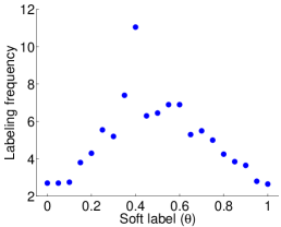
Refer to caption
(a) T=5K=105𝑇5𝐾105T=5K=105
Refer to caption
(b) T=15K=315𝑇15𝐾315T=15K=315
Refer to caption
(c) T=50K=1050𝑇50𝐾1050T=50K=1050
Figure 4: Labeling counts for instances with different levels of ambiguity.
Refer to caption
(a) T=5K=105𝑇5𝐾105T=5K=105
Refer to caption
(b) T=15K=315𝑇15𝐾315T=15K=315
Refer to caption
(c) T=50K=1050𝑇50𝐾1050T=50K=1050
Figure 5: Labeling counts for workers with different levels of reliability.

We first investigate that, in the homogeneous noiseless worker setting (i.e., workers are fully reliable), how the total budget is allocated among instances with different levels of ambiguity. In particular, we assume there are K=21𝐾21K=21 instances with soft-labels 𝜽=(θ1,θ2,θ3,,θK)=(0,0.05,0.1,,1)𝜽subscript𝜃1subscript𝜃2subscript𝜃3subscript𝜃𝐾00.050.11\bm{\theta}=(\theta_{1},\theta_{2},\theta_{3},\ldots,\theta_{K})=(0,0.05,0.1,\ldots,1). We vary the total budget T=5K,15K,50K𝑇5𝐾15𝐾50𝐾T=5K,15K,50K and report the number of times that each instance is labeled on average over 20 independent runs. The results are presented in Figure 4. It can be seen from Figure 4 that, more ambiguous instances with θ𝜃\theta close to 0.5 in general receive more labels than those simple instances with θ𝜃\theta close to 0 or 1. A more interesting observation is that when the budget level is low (e.g., T=5K𝑇5𝐾T=5K in Figure 4(a)), the policy spends less budget on those very ambiguous instances (e.g., θ=0.45𝜃0.45\theta=0.45 or 0.50.50.5 ), but more budget on exploring less ambiguous instances (e.g., θ=0.35𝜃0.35\theta=0.35, 0.40.40.4 or 0.60.60.6). When the budget goes higher (e.g., T=15K𝑇15𝐾T=15K in Figure 4(b)), those very ambiguous instances receive more labels but the most ambiguous instance (θ=0.5𝜃0.5\theta=0.5) not necessarily receives the most labels. In fact, the instances with θ=0.45𝜃0.45\theta=0.45 and θ=0.55𝜃0.55\theta=0.55 receive more labels than that of the most ambiguous instance. When the total budget is sufficiently large (e.g., T=50K𝑇50𝐾T=50K in Figure 4(c)), the most ambiguous instance receives the most labels since all the other instances have received enough labels to infer their true labels.

Next, we investigate that, in the heterogeneous worker setting, how many instances each worker is assigned. We simulate K=21𝐾21K=21 instances’ soft-labels as before and further simulate workers’ reliability 𝝆=(ρ1,ρ2,,ρM)=(0.1,0.15,,0.5,0.505,0.515,,0.995)𝝆subscript𝜌1subscript𝜌2subscript𝜌𝑀0.10.150.50.5050.5150.995\bm{\rho}=(\rho_{1},\rho_{2},\ldots,\rho_{M})=(0.1,0.15,\ldots,0.5,0.505,0.515,\ldots,0.995) for M=59𝑀59M=59 workers. Such a simulation ensures that there are more reliable workers, which is in line with actual situation. We vary the total budget T=5K,15K,50K𝑇5𝐾15𝐾50𝐾T=5K,15K,50K and report the number of instances that each worker is assigned on average over 20 independent runs in Figure 5. As one can see, when the budget level goes up, there is clear trend that more reliable workers receive more instances.

8.1.2 Prior for instances

We investigate how robust Opt-KG is when using the uniform prior for each θisubscript𝜃𝑖\theta_{i}. We first simulate K=50𝐾50K=50 instances with each θiBeta(0.5,0.5)similar-tosubscript𝜃𝑖Beta0.50.5\theta_{i}\sim\text{Beta}(0.5,0.5), θiBeta(2,2)similar-tosubscript𝜃𝑖Beta22\theta_{i}\sim\text{Beta}(2,2), θiBeta(2,1)similar-tosubscript𝜃𝑖Beta21\theta_{i}\sim\text{Beta}(2,1) or θiBeta(4,1)similar-tosubscript𝜃𝑖Beta41\theta_{i}\sim\text{Beta}(4,1). The density functions of these four different Beta distributions are plotted in Figure 6. For each generating distribution of θisubscript𝜃𝑖\theta_{i}, we compare Opt-KG using the uniform prior (Beta(1,1)Beta11\text{Beta}(1,1)) (in red line) to Opt-KG with the true generating distribution as the prior (in blue line). The comparison in accuracy with different levels of budget (T=2K,,20K𝑇2𝐾20𝐾T=2K,\ldots,20K) is shown in Figure 7. As we can see, the performance of Opt-KG using two different priors are quite similar for most generating distributions except for θiBeta(4,1)similar-tosubscript𝜃𝑖Beta41\theta_{i}\sim\text{Beta}(4,1) (i.e., the highly imbalanced class distribution). When θiBeta(4,1)similar-tosubscript𝜃𝑖Beta41\theta_{i}\sim\text{Beta}(4,1), the Opt-KG with uniform prior needs at least T=16K𝑇16𝐾T=16K units of budget to match the performance of Opt-KG with true generating distribution as the prior. This result indicates that for balanced class distributions, the uniform prior is a good choice and robust to the underlying distribution of θisubscript𝜃𝑖\theta_{i}. For highly imbalanced class distributions, if a uniform prior is adopted, one needs more budget to recover from the inaccurate prior belief.
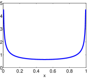
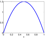
Refer to caption
(a) Beta(0.5,0.5)Beta0.50.5\text{Beta}(0.5,0.5)
Refer to caption
(b) Beta(2,2)Beta22\text{Beta}(2,2)
Refer to caption
(c) Beta(2,1)Beta21\text{Beta}(2,1)
Refer to caption
(d) Beta(4,1)Beta41\text{Beta}(4,1)
Figure 6: Density plot for different Beta distributions for generating each θisubscript𝜃𝑖\theta_{i}. Here, (a) represents there are more easier instances; (b) more ambiguous instances; (c) & (d) imbalanced class distributions with more positive instances.
Refer to caption
(a) θiBeta(0.5,0.5)similar-tosubscript𝜃𝑖Beta0.50.5\theta_{i}\sim\text{Beta}(0.5,0.5)
Refer to caption
(b) θiBeta(2,2)similar-tosubscript𝜃𝑖Beta22\theta_{i}\sim\text{Beta}(2,2)
Refer to caption
(c) θiBeta(2,1)similar-tosubscript𝜃𝑖Beta21\theta_{i}\sim\text{Beta}(2,1)
Refer to caption
(d) θiBeta(4,1)similar-tosubscript𝜃𝑖Beta41\theta_{i}\sim\text{Beta}(4,1)
Figure 7: Comparison between Opt-KG using the uniform distribution and true generating distribution as the prior.

8.1.3 Prior on workers

We investigate how sensitive the prior for the workers’ reliability ρjsubscript𝜌𝑗\rho_{j} is. In particular, we simulate K=50𝐾50K=50 instances with each θiBeta(1,1)similar-tosubscript𝜃𝑖Beta11\theta_{i}\sim\text{Beta}(1,1) and M=100𝑀100M=100 workers with ρjBeta(3,1)similar-tosubscript𝜌𝑗Beta31\rho_{j}\sim\text{Beta}(3,1), ρjBeta(8,1)similar-tosubscript𝜌𝑗Beta81\rho_{j}\sim\text{Beta}(8,1) or ρjBeta(5,2)similar-tosubscript𝜌𝑗Beta52\rho_{j}\sim\text{Beta}(5,2). We ensure that there are more reliable workers than spammers or poorly informed workers, which is in line with the actual situation. We use the prior Beta(4,1)Beta41\text{Beta}(4,1), which indicates that we have the prior belief that most workers preform reasonably well and the averaged accuracy is 4/5=80%45percent804/5=80\%. In Figure 8, we show different density functions for generating ρjsubscript𝜌𝑗\rho_{j} and the prior that we use (in Figure 8 (d)). For each generating distribution of θisubscript𝜃𝑖\theta_{i}, we compare the Opt-KG policy using the prior (Beta(4,1)Beta41\text{Beta}(4,1)) (in red line) to the Opt-KG with the true generating distribution as the prior (in blue line). The comparison in accuracy with different levels of budget (T=2K,,20K𝑇2𝐾20𝐾T=2K,\ldots,20K) is shown in Figure 9. From Figure 9, we observe that the performance of Opt-KG using two different priors are quite similar in all different settings. Hence, we will use Beta(4,1)Beta41\text{Beta}(4,1) as the prior when the true prior of workers is unavailable.
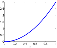
Refer to caption
(a) Beta(3,1)Beta31\text{Beta}(3,1)
Refer to caption
(b) Beta(8,1)Beta81\text{Beta}(8,1)
Refer to caption
(c) Beta(5,2)Beta52\text{Beta}(5,2)
Refer to caption
(d) Beta(4,1)Beta41\text{Beta}(4,1)
Figure 8: Density plot for different Beta distributions for generating ρjsubscript𝜌𝑗\rho_{j}. The plot in (d) is the one that we use as the prior.
Refer to caption
(a) θiBeta(3,1)similar-tosubscript𝜃𝑖Beta31\theta_{i}\sim\text{Beta}(3,1)
Refer to caption
(b) θiBeta(8,1)similar-tosubscript𝜃𝑖Beta81\theta_{i}\sim\text{Beta}(8,1)
Refer to caption
(c) θiBeta(5,2)similar-tosubscript𝜃𝑖Beta52\theta_{i}\sim\text{Beta}(5,2)
Figure 9: Comparison between Opt-KG using Beta(4,1)Beta41\text{Beta}(4,1) and true generating distribution prior as the prior.

8.1.4 Performance comparison under the homogeneous noiseless worker setting
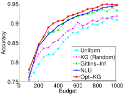
Refer to caption
(a) θiBeta(1,1)similar-tosubscript𝜃𝑖Beta11\theta_{i}\sim\text{Beta}(1,1) (True Prior)
Refer to caption
(b) θiBeta(0.5,0.5)similar-tosubscript𝜃𝑖Beta0.50.5\theta_{i}\sim\text{Beta}(0.5,0.5) (True Prior)
Refer to caption
(c) θiBeta(0.5,0.5)similar-tosubscript𝜃𝑖Beta0.50.5\theta_{i}\sim\text{Beta}(0.5,0.5) (Uni Prior)
Refer to caption
(d) θiBeta(2,2)similar-tosubscript𝜃𝑖Beta22\theta_{i}\sim\text{Beta}(2,2) (True Prior)
Refer to caption
(e) θiBeta(2,2)similar-tosubscript𝜃𝑖Beta22\theta_{i}\sim\text{Beta}(2,2) (Uni Prior)
Refer to caption
(f) θiBeta(2,1)similar-tosubscript𝜃𝑖Beta21\theta_{i}\sim\text{Beta}(2,1) (True Prior)
Refer to caption
(g) θiBeta(2,1)similar-tosubscript𝜃𝑖Beta21\theta_{i}\sim\text{Beta}(2,1) (Uni Prior)
Refer to caption
(h) θiBeta(4,1)similar-tosubscript𝜃𝑖Beta41\theta_{i}\sim\text{Beta}(4,1) (True Prior)
Refer to caption
(i) θiBeta(4,1)similar-tosubscript𝜃𝑖Beta41\theta_{i}\sim\text{Beta}(4,1) (Uni Prior)
Figure 10: Performance comparison under the homogeneous noiseless worker setting.

We compare the performance of Opt-KG under the homogeneous noiseless worker setting to several other competitors, including
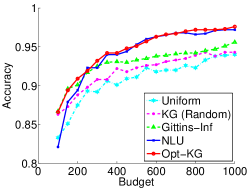
  1. 1.

    Uniform: Uniform sampling.

  2. 2.

    KG(Random): Randomized knowledge gradient [9].

  3. 3.

    Gittins-Inf: A Gittins-indexed based policy proposed in [39] for solving an infinite-horizon Bayesian MAB problem where the reward is discounted by δ𝛿\delta. Although it solves a different problem, we apply it as a heuristic by choosing the discount factor δ𝛿\delta such that T=1/(1δ)𝑇11𝛿T=1/(1-\delta).

  4. 4.

    NLU: The “new labeling uncertainty” method proposed in [15].

We note that we do not compare to the finite-horizon Gittins index rule [25] since its computation is very expensive. On some small-scale problems, we observe that the finite-horizon Gittins index rule [25] has the similar performance as Gittins-Inf in [39].

We simulate K=50𝐾50K=50 instances with each θiBeta(1,1)similar-tosubscript𝜃𝑖Beta11\theta_{i}\sim\text{Beta}(1,1), θiBeta(0.5,0.5)similar-tosubscript𝜃𝑖Beta0.50.5\theta_{i}\sim\text{Beta}(0.5,0.5), θiBeta(2,2)similar-tosubscript𝜃𝑖Beta22\theta_{i}\sim\text{Beta}(2,2), θiBeta(2,1)similar-tosubscript𝜃𝑖Beta21\theta_{i}\sim\text{Beta}(2,1) or θiBeta(4,1)similar-tosubscript𝜃𝑖Beta41\theta_{i}\sim\text{Beta}(4,1) (see Figure 6). For each of the five settings, we vary the total budget T=2K,3K,,20K𝑇2𝐾3𝐾20𝐾T=2K,3K,\ldots,20K and report the mean of accuracy for 20 independently generated sets of {θi}i=1Ksuperscriptsubscriptsubscript𝜃𝑖𝑖1𝐾\{\theta_{i}\}_{i=1}^{K}. For the last four settings, we report the comparison among different methods when either using the uniform prior (“uni prior” for short) or the true generating distribution as the prior. From Figure 10, the proposed Opt-KG outperforms all the other competitors in most settings regardless the choice of the prior. For θiBeta(0.5,0.5)similar-tosubscript𝜃𝑖Beta0.50.5\theta_{i}\sim\text{Beta}(0.5,0.5), NLU matches the performance of Opt-KG; and for θiBeta(2,2)similar-tosubscript𝜃𝑖Beta22\theta_{i}\sim\text{Beta}(2,2), Gittins-inf matches the performance of Opt-KG. We also observe that the performance of randomized KG only slightly improves that of uniform sampling.

8.1.5 Performance comparison under the heterogeneous worker setting

We compare the proposed Opt-KG under the heterogeneous worker setting to several other competitors:

  1. 1.

    Uniform: Uniform sampling.

  2. 2.

    KG(Random): Randomized knowledge gradient [9].

  3. 3.

    KOS: The randomized budget allocation algorithm in [19].

We note that several competitors for the homogeneous worker setting (e.g., Gittins-inf and NLU) cannot be directly applied to the heterogeneous worker setting since they fail to model each worker’s reliability.
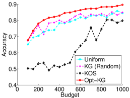
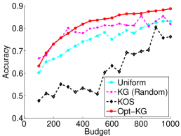
Refer to caption
(a) ρjBeta(4,1)similar-tosubscript𝜌𝑗Beta41\rho_{j}\sim\text{Beta}(4,1) (True Prior)
Refer to caption
(b) ρjBeta(3,1)similar-tosubscript𝜌𝑗Beta31\rho_{j}\sim\text{Beta}(3,1) (True Prior)
Refer to caption
(c) ρjBeta(3,1)similar-tosubscript𝜌𝑗Beta31\rho_{j}\sim\text{Beta}(3,1) (Beta(4,1)Beta41\text{Beta}(4,1) Prior)
Refer to caption
(d) ρjBeta(8,1)similar-tosubscript𝜌𝑗Beta81\rho_{j}\sim\text{Beta}(8,1) (True Prior)
Refer to caption
(e) ρjBeta(8,1)similar-tosubscript𝜌𝑗Beta81\rho_{j}\sim\text{Beta}(8,1) (Beta(4,1)Beta41\text{Beta}(4,1) Prior)
Refer to caption
(f) ρjBeta(5,2)similar-tosubscript𝜌𝑗Beta52\rho_{j}\sim\text{Beta}(5,2) (True Prior)
Refer to caption
(g) ρjBeta(5,2)similar-tosubscript𝜌𝑗Beta52\rho_{j}\sim\text{Beta}(5,2) (Beta(4,1)Beta41\text{Beta}(4,1) Prior)
Figure 11: Performance comparison under the heterogeneous worker setting.

We simulate K=50𝐾50K=50 instances with each θiBeta(1,1)similar-tosubscript𝜃𝑖Beta11\theta_{i}\sim\text{Beta}(1,1) and M=100𝑀100M=100 workers with ρjBeta(4,1)similar-tosubscript𝜌𝑗Beta41\rho_{j}\sim\text{Beta}(4,1), ρjBeta(3,1)similar-tosubscript𝜌𝑗Beta31\rho_{j}\sim\text{Beta}(3,1), ρjBeta(8,1)similar-tosubscript𝜌𝑗Beta81\rho_{j}\sim\text{Beta}(8,1) or ρjBeta(5,2)similar-tosubscript𝜌𝑗Beta52\rho_{j}\sim\text{Beta}(5,2) (see Figure 8). For each of the four settings, we vary the total budget T=2K,3K,,20K𝑇2𝐾3𝐾20𝐾T=2K,3K,\ldots,20K and report the mean of accuracy for 20 independently generated sets of parameters. For the last three settings, we report the comparison among different methods when either using Beta(4,1)Beta41\text{Beta}(4,1) prior or the true generating distribution for ρjsubscript𝜌𝑗\rho_{j} as the prior. From Figure 11, the proposed Opt-KG outperforms all the other competitors regardless the choice of the prior.

8.2 Real Data

We compare different policies on a standard real dataset for recognizing textual entailment (RTE) (Section 4.3 in [34]). There are 800 instances and each instance is a sentence pair. Each sentence pair is presented to 10 different workers to acquire binary choices of whether the second hypothesis sentence can be inferred from the first one. There are in total 164 different workers. We first consider the homogeneous noiseless setting without incorporating the diversity of workers and use the uniform prior (Beta(1,1)Beta11\text{Beta}(1,1)) for each θisubscript𝜃𝑖\theta_{i}. In such a setting, once we decide to label an instance, we randomly choose a worker (who provides the label in the full dataset) to acquire the label. Due to this randomness, we run each policy 20 times and report the mean of the accuracy in Figure 12(a). As we can see, Opt-KG, Gittins-inf and NLU all perform quite well. We also note that although Gittins-inf performs slightly better than our method on this data, it requires solving a linear system with O(T2)𝑂superscript𝑇2O(T^{2}) variables at each stage, which could be too expensive for large-scale applications. While our Opt-KG policy has a time complexity linear in KT𝐾𝑇KT and space complexity linear in K𝐾K, which is much more efficient when a quick online decision is required. In particular, we present the comparison between Opt-KG and Gittins-inf on the averaged CPU time under different budget levels in Table 4. As one can see, Gittins-inf is computationally more expensive than Opt-KG.
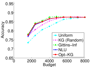
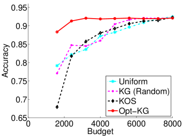
Refer to caption
(a) RTE: Homogeneous Noiseless Worker
Refer to caption
(b) RTE: Heterogeneous Worker
Figure 12: Performance comparison on the real dataset.
Table 4: Comparison in CPU time (seconds)
Budget T𝑇T 2K=1,6002𝐾16002K=1,600 4K=3,2004𝐾32004K=3,200 6K=4,8006𝐾48006K=4,800 10K=8,00010𝐾800010K=8,000
Opt-KG 1.09 2.19 3.29 5.48
Gittins-inf 25.87 35.70 45.59 130.68

When the worker reliability is incorporated, we compare different policies in Figure 12(b). We put Beta(4,1)Beta41\text{Beta}(4,1) prior distribution for each ρjsubscript𝜌𝑗\rho_{j} which indicates that we have the prior belief that most workers perform reasonably well. Other priors in Figure 8 lead to similar results and thus omitted here. As one can see, the accuracy of Opt-KG is much higher than that of other policies when T𝑇T is small. It achieves the highest accuracy of 92.05%percent92.0592.05\% only using 40% of the total budget (i.e., on average, each instance is labeled 4 times). One may also observe that when T>4K=3,200formulae-sequence𝑇4𝐾3200T>4K=3,200, the performance of Opt-KG does not improve and in fact, slightly downgrades a little bit. This is mainly due to the restrictiveness of the experimental setting. In particular, since the experiment is conducted on a fixed dataset with partially observed labels, the Opt-KG cannot freely choose instance-worker pairs especially when the budget goes up (i.e., the action set is greatly restricted). According to our experience, such a phenomenon will not happen on experiments when labels can be obtained from any instance-worker pair. Comparing Figure 12(b) to 12(a), we also observe that Opt-KG under the heterogeneous worker setting performs much better than Opt-KG under the homogeneous worker setting, which indicates that it is beneficial to incorporate workers’ reliability.

9 Conclusions and Future Works

In this paper, we propose to address the problem of budget allocation in crowd labeling. We model the problem using the Bayesian Markov decision process and characterize the optimal policy using the dynamic programming. We further propose a computationally more attractive approximate policy: optimistic knowledge gradient. Our MDP formulation is a general framework, which can be applied to binary or multi-class, contextual or non-contextual crowd labeling problems in either pull or push crowdsourcing marketplaces.

There are several possible future directions for this work. First, it is of great interest to show the consistency of Opt-KG in heterogonous worker setting and further provide the theoretical results on the performance of Opt-KG under finite budget. Second, in this work, we assume that both instances and workers are equally priced. Although this assumption is standard in many crowd labeling applications, a dynamic pricing strategy as the allocation process proceeds will better motivate those more reliable workers to label more challenge instances. A recent work in [36] provides some quality-based pricing algorithms for crowd workers and it will be interesting to incorporate their strategies into our dynamic allocation framework. Third, we assume that the labels provided by the same worker to different instances are independent. It is more interesting to consider that the workers’ reliability will be improved during the labeling process when some useful feedback can be provided. Further, since the proposed Opt-KG is a fairly general approximate policy for MDP, it is also interesting to apply it to other statistical decision problems.

10 Acknowledgement

We would like to thank Qiang Liu for sharing the code for KOS method; Jing Xie and Peter Frazier for sharing their code for computing infinite-horizon Gittins index; John Platt, Chris J.C. Burges and Kevin P. Murphy for helpful discussions; and anonymous reviewers and the associate editor for their constructive comments on improving the quality of the paper.

Appendix

Proof of Proposition 3.1

The final positive set HTsubscript𝐻𝑇H_{T} is chosen to maximize the expected accuracy conditioned on Tsubscript𝑇\mathcal{F}_{T}:

HT=argmaxH𝔼(i=1K(𝟏(iH)𝟏(iH)+𝟏(iH)𝟏(iH))|T)subscript𝐻𝑇subscriptargmax𝐻𝔼conditionalsuperscriptsubscript𝑖1𝐾1𝑖𝐻1𝑖superscript𝐻1𝑖𝐻1𝑖superscript𝐻subscript𝑇H_{T}=\mathop{\mathrm{arg\,max}{}}_{H}\mathbb{E}\left(\sum_{i=1}^{K}\left(\mathbf{1}(i\in H)\mathbf{1}(i\in H^{*})+\mathbf{1}(i\not\in H)\mathbf{1}(i\not\in H^{*})\right)\Bigg{|}\mathcal{F}_{T}\right) (24)

According to the definition (6) of PiTsubscriptsuperscript𝑃𝑇𝑖P^{T}_{i}, we can re-write (24) using the linearity of the expectation:

i=1K(𝟏(iH)Pr(iH|T)+𝟏(iH)Pr(iH|T))superscriptsubscript𝑖1𝐾1𝑖𝐻Pr𝑖conditionalsuperscript𝐻subscript𝑇1𝑖𝐻Pr𝑖conditionalsuperscript𝐻subscript𝑇\displaystyle\sum_{i=1}^{K}\left(\mathbf{1}(i\in H)\Pr(i\in H^{*}|\mathcal{F}_{T})+\mathbf{1}(i\not\in H)\Pr(i\not\in H^{*}|\mathcal{F}_{T})\right)
=\displaystyle= i=1K(𝟏(iH)PiT+𝟏(iH)(1PiT))superscriptsubscript𝑖1𝐾1𝑖𝐻superscriptsubscript𝑃𝑖𝑇1𝑖𝐻1superscriptsubscript𝑃𝑖𝑇\displaystyle\sum_{i=1}^{K}\left(\mathbf{1}(i\in H)P_{i}^{T}+\mathbf{1}(i\not\in H)(1-P_{i}^{T})\right) (25)

To maximize (25) over H𝐻H, it easy to see that we should set iH𝑖𝐻i\in H if and only if PiT0.5superscriptsubscript𝑃𝑖𝑇0.5P_{i}^{T}\geq 0.5. Therefore, we have the positive set

HT={i:PiT0.5}.subscript𝐻𝑇conditional-set𝑖superscriptsubscript𝑃𝑖𝑇0.5H_{T}=\{i:P_{i}^{T}\geq 0.5\}.

Proof of Corollary 3.2

Recall that

I(a,b)=Pr(θ0.5|θBeta(a,b))=1B(a,b)0.51ta1(1t)b1dt,𝐼𝑎𝑏Pr𝜃conditional0.5𝜃similar-toBeta𝑎𝑏1𝐵𝑎𝑏superscriptsubscript0.51superscript𝑡𝑎1superscript1𝑡𝑏1differential-d𝑡\displaystyle I(a,b)=\Pr(\theta\geq 0.5|\theta\sim\mathrm{Beta}(a,b))=\frac{1}{B(a,b)}\int_{0.5}^{1}t^{a-1}(1-t)^{b-1}\mathrm{d}t, (26)

where B(a,b)𝐵𝑎𝑏B(a,b) is the beta function.

It is easy to see that I(a,b)>0.5I(a,b)>1I(a,b)𝐼𝑎𝑏0.5𝐼𝑎𝑏1𝐼𝑎𝑏I(a,b)>0.5\Longleftrightarrow I(a,b)>1-I(a,b). We re-write 1I(a,b)1𝐼𝑎𝑏1-I(a,b) as follows

1I(a,b)=1B(a,b)00.5ta1(1t)b1dt=1B(a,b)0.51tb1(1t)a1dt,1𝐼𝑎𝑏1𝐵𝑎𝑏superscriptsubscript00.5superscript𝑡𝑎1superscript1𝑡𝑏1differential-d𝑡1𝐵𝑎𝑏superscriptsubscript0.51superscript𝑡𝑏1superscript1𝑡𝑎1differential-d𝑡\displaystyle 1-I(a,b)=\frac{1}{B(a,b)}\int_{0}^{0.5}t^{a-1}(1-t)^{b-1}\mathrm{d}t=\frac{1}{B(a,b)}\int_{0.5}^{1}t^{b-1}(1-t)^{a-1}\mathrm{d}t,

where the second equality is obtained by setting t:=1tassign𝑡1𝑡t:=1-t. Then we have:

I(a,b)(1I(a,b))𝐼𝑎𝑏1𝐼𝑎𝑏\displaystyle I(a,b)-(1-I(a,b)) =\displaystyle= 1B(a,b)0.51(ta1(1t)b1tb1(1t)a1)dt1𝐵𝑎𝑏superscriptsubscript0.51superscript𝑡𝑎1superscript1𝑡𝑏1superscript𝑡𝑏1superscript1𝑡𝑎1differential-d𝑡\displaystyle\frac{1}{B(a,b)}\int_{0.5}^{1}(t^{a-1}(1-t)^{b-1}-t^{b-1}(1-t)^{a-1})\mathrm{d}t
=\displaystyle= 1B(a,b)0.51ta1(1t)b1((t1t)ab1)dt1𝐵𝑎𝑏superscriptsubscript0.51superscript𝑡𝑎1superscript1𝑡𝑏1superscript𝑡1𝑡𝑎𝑏1differential-d𝑡\displaystyle\frac{1}{B(a,b)}\int_{0.5}^{1}t^{a-1}(1-t)^{b-1}\left(\left(\frac{t}{1-t}\right)^{a-b}-1\right)\mathrm{d}t

Since t>0.5𝑡0.5t>0.5, t1t>1𝑡1𝑡1\frac{t}{1-t}>1. When a>b𝑎𝑏a>b, (t1t)ab>1superscript𝑡1𝑡𝑎𝑏1\left(\frac{t}{1-t}\right)^{a-b}>1 and hence I(a,b)(1I(a,b))>0𝐼𝑎𝑏1𝐼𝑎𝑏0I(a,b)-(1-I(a,b))>0, i.e, I(a,b)>0.5𝐼𝑎𝑏0.5I(a,b)>0.5. When a=b𝑎𝑏a=b, (t1t)ab1superscript𝑡1𝑡𝑎𝑏1\left(\frac{t}{1-t}\right)^{a-b}\equiv 1 and I(a,b)=0.5𝐼𝑎𝑏0.5I(a,b)=0.5. When a<b𝑎𝑏a<b, (t1t)ab<1superscript𝑡1𝑡𝑎𝑏1\left(\frac{t}{1-t}\right)^{a-b}<1 and I(a,b)<0.5𝐼𝑎𝑏0.5I(a,b)<0.5.

Proof of Proposition 3.3

We use the proof technique in [39] to prove Proposition 3.3. According to (8), the value function takes the following form,

V(S0)=supπ𝔼π(i=1Kh(PiT)).𝑉superscript𝑆0subscriptsupremum𝜋superscript𝔼𝜋superscriptsubscript𝑖1𝐾superscriptsubscript𝑃𝑖𝑇\displaystyle V(S^{0})=\sup_{\pi}\mathbb{E}^{\pi}\left(\sum_{i=1}^{K}h(P_{i}^{T})\right). (27)

To decompose the final accuracy i=1Kh(PiT)superscriptsubscript𝑖1𝐾superscriptsubscript𝑃𝑖𝑇\sum_{i=1}^{K}h(P_{i}^{T}) into the incremental reward at each stage, we define G0=i=1Kh(Pi0)subscript𝐺0superscriptsubscript𝑖1𝐾superscriptsubscript𝑃𝑖0G_{0}=\sum_{i=1}^{K}h(P_{i}^{0}) and Gt+1=i=1Kh(Pit+1)i=1Kh(Pit)subscript𝐺𝑡1superscriptsubscript𝑖1𝐾superscriptsubscript𝑃𝑖𝑡1superscriptsubscript𝑖1𝐾superscriptsubscript𝑃𝑖𝑡G_{t+1}=\sum_{i=1}^{K}h(P_{i}^{t+1})-\sum_{i=1}^{K}h(P_{i}^{t}). Then, i=1Kh(PiT)superscriptsubscript𝑖1𝐾superscriptsubscript𝑃𝑖𝑇\sum_{i=1}^{K}h(P_{i}^{T}) can be decomposed as: i=1Kh(PiT)G0+t=0T1Gt+1superscriptsubscript𝑖1𝐾superscriptsubscript𝑃𝑖𝑇subscript𝐺0superscriptsubscript𝑡0𝑇1subscript𝐺𝑡1\sum_{i=1}^{K}h(P_{i}^{T})\equiv G_{0}+\sum_{t=0}^{T-1}G_{t+1}. The value function can now be re-written as follows:

V(S0)𝑉superscript𝑆0\displaystyle V(S^{0}) =\displaystyle= G0(S0)+supπt=0T1𝔼π(Gt+1)subscript𝐺0superscript𝑆0subscriptsupremum𝜋superscriptsubscript𝑡0𝑇1superscript𝔼𝜋subscript𝐺𝑡1\displaystyle G_{0}(S^{0})+\sup_{\pi}\sum_{t=0}^{T-1}\mathbb{E}^{\pi}(G_{t+1})
=\displaystyle= G0(S0)+supπt=0T1𝔼π(𝔼(Gt+1|t))subscript𝐺0superscript𝑆0subscriptsupremum𝜋superscriptsubscript𝑡0𝑇1superscript𝔼𝜋𝔼conditionalsubscript𝐺𝑡1subscript𝑡\displaystyle G_{0}(S^{0})+\sup_{\pi}\sum_{t=0}^{T-1}\mathbb{E}^{\pi}\left(\mathbb{E}(G_{t+1}|\mathcal{F}_{t})\right)
=\displaystyle= G0(S0)+supπt=0T1𝔼π(𝔼(Gt+1|St,it)).subscript𝐺0superscript𝑆0subscriptsupremum𝜋superscriptsubscript𝑡0𝑇1superscript𝔼𝜋𝔼conditionalsubscript𝐺𝑡1superscript𝑆𝑡subscript𝑖𝑡\displaystyle G_{0}(S^{0})+\sup_{\pi}\sum_{t=0}^{T-1}\mathbb{E}^{\pi}\left(\mathbb{E}(G_{t+1}|S^{t},i_{t})\right).

Here, the first inequality is true because G0subscript𝐺0G_{0} is determinant and independent of π𝜋\pi; the second inequality is due to the tower property of conditional expectation and the third one holds because Gt+1subscript𝐺𝑡1G_{t+1}, which is a function of Pit+1superscriptsubscript𝑃𝑖𝑡1P_{i}^{t+1} and Pitsuperscriptsubscript𝑃𝑖𝑡P_{i}^{t}, depends on tsubscript𝑡\mathcal{F}_{t} only through Stsuperscript𝑆𝑡S^{t} and itsubscript𝑖𝑡i_{t}. We define incremental expected reward gained by labeling the itsubscript𝑖𝑡i_{t}-th instance at the state Stsuperscript𝑆𝑡S^{t} as follows:

R(St,it)𝑅superscript𝑆𝑡subscript𝑖𝑡\displaystyle R(S^{t},i_{t}) =\displaystyle= 𝔼(Gt+1|St,it)=𝔼(i=1Kh(Pit+1)i=1Kh(Pit)|St,it)𝔼conditionalsubscript𝐺𝑡1superscript𝑆𝑡subscript𝑖𝑡𝔼superscriptsubscript𝑖1𝐾superscriptsubscript𝑃𝑖𝑡1conditionalsuperscriptsubscript𝑖1𝐾superscriptsubscript𝑃𝑖𝑡superscript𝑆𝑡subscript𝑖𝑡\displaystyle\mathbb{E}(G_{t+1}|S^{t},i_{t})=\mathbb{E}\left(\sum_{i=1}^{K}h(P_{i}^{t+1})-\sum_{i=1}^{K}h(P_{i}^{t})|S^{t},i_{t}\right) (28)
=\displaystyle= 𝔼(h(Pitt+1)h(Pitt)|St,it).𝔼superscriptsubscript𝑃subscript𝑖𝑡𝑡1conditionalsuperscriptsubscript𝑃subscript𝑖𝑡𝑡superscript𝑆𝑡subscript𝑖𝑡\displaystyle\mathbb{E}\left(h(P_{i_{t}}^{t+1})-h(P_{i_{t}}^{t})|S^{t},i_{t}\right).

The last equation is due to the fact that only Pittsuperscriptsubscript𝑃subscript𝑖𝑡𝑡P_{i_{t}}^{t} will be changed if the itsubscript𝑖𝑡i_{t}-th instance is labeled next. With the expected reward function in place, the value function in (8) can be re-formulated as:

V(S0)=G0(𝐬)+supπ𝔼π(t=0T1R(St,it)|S0).𝑉superscript𝑆0subscript𝐺0𝐬subscriptsupremum𝜋superscript𝔼𝜋conditionalsuperscriptsubscript𝑡0𝑇1𝑅superscript𝑆𝑡subscript𝑖𝑡superscript𝑆0V(S^{0})=G_{0}(\mathbf{s})+\sup_{\pi}\mathbb{E}^{\pi}\left(\sum_{t=0}^{T-1}R(S^{t},i_{t})\Big{|}S^{0}\right). (29)

Proof of Proposition 4.1

To prove the failure of deterministic KG, we first show a key property for the expected reward function:

R(a,b)=aa+b(h(I(a+1,b))h(I(a,b)))+ba+b(h(I(a,b+1))h(I(a,b))).𝑅𝑎𝑏𝑎𝑎𝑏𝐼𝑎1𝑏𝐼𝑎𝑏𝑏𝑎𝑏𝐼𝑎𝑏1𝐼𝑎𝑏\displaystyle R(a,b)=\frac{a}{a+b}\left(h(I(a+1,b))-h(I(a,b))\right)+\frac{b}{a+b}\left(h(I(a,b+1))-h(I(a,b))\right). (30)
Lemma .1

When a,b𝑎𝑏a,b are positive integers, if a=b𝑎𝑏a=b, R(a,b)=0.52aaB(a,a)𝑅𝑎𝑏superscript0.52𝑎𝑎𝐵𝑎𝑎R(a,b)=\frac{0.5^{2a}}{aB(a,a)} and if ab𝑎𝑏a\neq b, R(a,b)=0𝑅𝑎𝑏0R(a,b)=0.

To prove lemma .1, we first present several basic properties for B(a,b)𝐵𝑎𝑏B(a,b) and I(a,b)𝐼𝑎𝑏I(a,b), which will be used in all the following theorems and proofs.

  1. 1.

    Properties for B(a,b)𝐵𝑎𝑏B(a,b):

    B(a,b)=B(b,a)𝐵𝑎𝑏𝐵𝑏𝑎\displaystyle B(a,b)=B(b,a) (31)
    B(a+1,b)=aa+bB(a,b)𝐵𝑎1𝑏𝑎𝑎𝑏𝐵𝑎𝑏\displaystyle B(a+1,b)=\frac{a}{a+b}B(a,b) (32)
    B(a,b+1)=ba+bB(a,b)𝐵𝑎𝑏1𝑏𝑎𝑏𝐵𝑎𝑏\displaystyle B(a,b+1)=\frac{b}{a+b}B(a,b) (33)
  2. 2.

    Properties for B(a,b)𝐵𝑎𝑏B(a,b):

    I(a,b)=1I(b,a)𝐼𝑎𝑏1𝐼𝑏𝑎\displaystyle I(a,b)=1-I(b,a) (34)
    I(a+1,b)=I(a,b)+0.5a+baB(a,b)𝐼𝑎1𝑏𝐼𝑎𝑏superscript0.5𝑎𝑏𝑎𝐵𝑎𝑏\displaystyle I(a+1,b)=I(a,b)+\frac{0.5^{a+b}}{aB(a,b)} (35)
    I(a,b+1)=I(a,b)0.5a+bbB(a,b)𝐼𝑎𝑏1𝐼𝑎𝑏superscript0.5𝑎𝑏𝑏𝐵𝑎𝑏\displaystyle I(a,b+1)=I(a,b)-\frac{0.5^{a+b}}{bB(a,b)} (36)

    The properties for I(a,b)𝐼𝑎𝑏I(a,b) are derived from the basic property of regularized incomplete beta function 333http://dlmf.nist.gov/8.17.

  • Proof of Lemma .1

When a=b𝑎𝑏a=b, by Corollary 3.2, we have I(a+1,b)>0.5𝐼𝑎1𝑏0.5I(a+1,b)>0.5, I(a,b)=0.5𝐼𝑎𝑏0.5I(a,b)=0.5 and I(a,b+1)<0.5𝐼𝑎𝑏10.5I(a,b+1)<0.5. Therefore, the expected reward (30) takes the following form:

R(a,b)𝑅𝑎𝑏\displaystyle R(a,b) =\displaystyle= 0.5(I(a+1,a)I(a,a))+0.5((1I(a,a+1))I(a,a))0.5𝐼𝑎1𝑎𝐼𝑎𝑎0.51𝐼𝑎𝑎1𝐼𝑎𝑎\displaystyle 0.5(I(a+1,a)-I(a,a))+0.5((1-I(a,a+1))-I(a,a))
=\displaystyle= I(a+1,a)I(a,a)=0.52aaB(a,a)𝐼𝑎1𝑎𝐼𝑎𝑎superscript0.52𝑎𝑎𝐵𝑎𝑎\displaystyle I(a+1,a)-I(a,a)=\frac{0.5^{2a}}{aB(a,a)}

When a>b𝑎𝑏a>b, since a,b𝑎𝑏a,b are integers, we have ab+1𝑎𝑏1a\geq b+1 and hence I(a+1,b)>0.5,I(a,b)>0.5,I(a,b+1)0.5formulae-sequence𝐼𝑎1𝑏0.5formulae-sequence𝐼𝑎𝑏0.5𝐼𝑎𝑏10.5I(a+1,b)>0.5,I(a,b)>0.5,I(a,b+1)\geq 0.5 according to Corollary 3.2. The expected reward (30) now becomes:

R(a,b)=𝑅𝑎𝑏absent\displaystyle R(a,b)= aa+bI(a+1,b)+ba+bI(a,b+1)I(a,b)𝑎𝑎𝑏𝐼𝑎1𝑏𝑏𝑎𝑏𝐼𝑎𝑏1𝐼𝑎𝑏\displaystyle\frac{a}{a+b}I(a+1,b)+\frac{b}{a+b}I(a,b+1)-I(a,b)
=\displaystyle= aa+b1B(a+1,b)0.51tta1(1t)b1dt𝑎𝑎𝑏1𝐵𝑎1𝑏superscriptsubscript0.51𝑡superscript𝑡𝑎1superscript1𝑡𝑏1differential-d𝑡\displaystyle\frac{a}{a+b}\frac{1}{B(a+1,b)}\int_{0.5}^{1}t\cdot t^{a-1}(1-t)^{b-1}\mathrm{d}t
+ba+b1B(a,b+1)0.51ta1(1t)(1t)b1dtI(a,b)𝑏𝑎𝑏1𝐵𝑎𝑏1superscriptsubscript0.51superscript𝑡𝑎11𝑡superscript1𝑡𝑏1differential-d𝑡𝐼𝑎𝑏\displaystyle+\frac{b}{a+b}\frac{1}{B(a,b+1)}\int_{0.5}^{1}\ t^{a-1}(1-t)(1-t)^{b-1}\mathrm{d}t-I(a,b)
=\displaystyle= 1B(a,b)0.51(t+(1t))ta1(1t)b1dtI(a,b)1𝐵𝑎𝑏superscriptsubscript0.51𝑡1𝑡superscript𝑡𝑎1superscript1𝑡𝑏1differential-d𝑡𝐼𝑎𝑏\displaystyle\frac{1}{B(a,b)}\int_{0.5}^{1}(t+(1-t))\cdot t^{a-1}(1-t)^{b-1}\mathrm{d}t-I(a,b)
=\displaystyle= I(a,b)I(a,b)=0.𝐼𝑎𝑏𝐼𝑎𝑏0\displaystyle I(a,b)-I(a,b)=0.

Here we use (32) and (33) to show that aa+b1B(a+1,b)=ba+b1B(a,b+1)=1B(a,b)𝑎𝑎𝑏1𝐵𝑎1𝑏𝑏𝑎𝑏1𝐵𝑎𝑏11𝐵𝑎𝑏\frac{a}{a+b}\frac{1}{B(a+1,b)}=\frac{b}{a+b}\frac{1}{B(a,b+1)}=\frac{1}{B(a,b)}.

When ab1𝑎𝑏1a\leq b-1, we can prove R(a,b)=0𝑅𝑎𝑏0R(a,b)=0 in a similar way.

With Lemma .1 in place, the proof for Proposition 4.1 is straightforward. Recall that the deterministic KG policy chooses the next instance according to

it=argmaxiR(St,i)=argmaxiR(ait,bit),subscript𝑖𝑡subscriptargmax𝑖𝑅superscript𝑆𝑡𝑖subscriptargmax𝑖𝑅superscriptsubscript𝑎𝑖𝑡superscriptsubscript𝑏𝑖𝑡i_{t}=\mathop{\mathrm{arg\,max}{}}_{i}R(S^{t},i)=\mathop{\mathrm{arg\,max}{}}_{i}R(a_{i}^{t},b_{i}^{t}),

and breaks the tie by selecting the one with the smallest index. Since R(a,b)>0𝑅𝑎𝑏0R(a,b)>0 if and only if a=b𝑎𝑏a=b, at the initial stage t=0𝑡0t=0, R(ai0,bi0)>0𝑅superscriptsubscript𝑎𝑖0superscriptsubscript𝑏𝑖00R(a_{i}^{0},b_{i}^{0})>0 for those instances i={i:ai0=bi0}𝑖conditional-set𝑖superscriptsubscript𝑎𝑖0superscriptsubscript𝑏𝑖0i\in\mathcal{E}=\{i:a_{i}^{0}=b_{i}^{0}\}. The policy will first select i0subscript𝑖0i_{0}\in\mathcal{E} with the largest R(ai0,bi0)𝑅superscriptsubscript𝑎𝑖0superscriptsubscript𝑏𝑖0R(a_{i}^{0},b_{i}^{0}). After obtaining the label yi0subscript𝑦subscript𝑖0y_{i_{0}}, either ai00superscriptsubscript𝑎subscript𝑖00a_{i_{0}}^{0} or bi00superscriptsubscript𝑏subscript𝑖00b_{i_{0}}^{0} will add one and hence ai01bi01superscriptsubscript𝑎subscript𝑖01superscriptsubscript𝑏subscript𝑖01a_{i_{0}}^{1}\neq b_{i_{0}}^{1} and R(ai01,bi01)=0𝑅superscriptsubscript𝑎subscript𝑖01superscriptsubscript𝑏subscript𝑖010R(a_{i_{0}}^{1},b_{i_{0}}^{1})=0. The policy will select another instance i1subscript𝑖1i_{1}\in\mathcal{E} with the “current” largest expected reward and the expected reward for i1subscript𝑖1i_{1} after obtaining the label yi1subscript𝑦subscript𝑖1y_{i_{1}} will then become zero. As a consequence, the KG policy will label each instance in \mathcal{E} for the first |||\mathcal{E}| stages and R(ai||,bi||)=0𝑅superscriptsubscript𝑎𝑖superscriptsubscript𝑏𝑖0R(a_{i}^{|\mathcal{E}|},b_{i}^{|\mathcal{E}|})=0 for all i{1,,K}𝑖1𝐾i\in\{1,\ldots,K\}. Then the deterministic policy will break the tie selecting the first instance to label. From now on, for any t||𝑡t\geq|\mathcal{E}|, if a1tb1tsuperscriptsubscript𝑎1𝑡superscriptsubscript𝑏1𝑡a_{1}^{t}\neq b_{1}^{t}, then the expected reward R(a1t,b1t)=0𝑅superscriptsubscript𝑎1𝑡superscriptsubscript𝑏1𝑡0R(a_{1}^{t},b_{1}^{t})=0. Since the expected reward for other instances are all zero, the policy will still label the first instance. On the other hand, if a1t=b1tsuperscriptsubscript𝑎1𝑡superscriptsubscript𝑏1𝑡a_{1}^{t}=b_{1}^{t}, and the first instance is the only one with the positive expected reward and the policy will label it. Thus Proposition 4.1 is proved.

  • Remark

    For randomized KG, after getting one label for each instance in \mathcal{E} for the first |||\mathcal{E}| stages, the expected reward for each instance has become zero. Then randomized KG will uniformly select one instance to label. At any stage t||𝑡t\geq|\mathcal{E}|, if there exists one instance i𝑖i (at most one instance) with ait=bitsuperscriptsubscript𝑎𝑖𝑡superscriptsubscript𝑏𝑖𝑡a_{i}^{t}=b_{i}^{t}, the KG policy will provide the next label for i𝑖i; otherwise, it will randomly select an instance to label.

Proof of Theorem 4.2

To prove the consistency of the Opt-KG policy, we first show the exact values for Rα+(a,b)=max(R1(a,b),R2(a,b))subscriptsuperscript𝑅𝛼𝑎𝑏subscript𝑅1𝑎𝑏subscript𝑅2𝑎𝑏R^{+}_{\alpha}(a,b)=\max(R_{1}(a,b),R_{2}(a,b)).

  1. 1.

    When ab+1𝑎𝑏1a\geq b+1:

    R1(a,b)subscript𝑅1𝑎𝑏\displaystyle R_{1}(a,b) =I(a+1,b)I(a,b)=0.5a+baB(a,b)>0;absent𝐼𝑎1𝑏𝐼𝑎𝑏superscript0.5𝑎𝑏𝑎𝐵𝑎𝑏0\displaystyle=I(a+1,b)-I(a,b)=\frac{0.5^{a+b}}{aB(a,b)}>0;
    R2(a,b)subscript𝑅2𝑎𝑏\displaystyle R_{2}(a,b) =I(a,b+1)I(a,b)=0.5a+bbB(a,b)<0.absent𝐼𝑎𝑏1𝐼𝑎𝑏superscript0.5𝑎𝑏𝑏𝐵𝑎𝑏0\displaystyle=I(a,b+1)-I(a,b)=-\frac{0.5^{a+b}}{bB(a,b)}<0.

    Therefore,

    R+(a,b)=R1(a,b)=0.5a+baB(a,b)>0.superscript𝑅𝑎𝑏subscript𝑅1𝑎𝑏superscript0.5𝑎𝑏𝑎𝐵𝑎𝑏0R^{+}(a,b)=R_{1}(a,b)=\frac{0.5^{a+b}}{aB(a,b)}>0.
  2. 2.

    When a=b𝑎𝑏a=b:

    R1(a,b)subscript𝑅1𝑎𝑏\displaystyle R_{1}(a,b) =I(a+1,a)I(a,a)=0.52aaB(a,a);absent𝐼𝑎1𝑎𝐼𝑎𝑎superscript0.52𝑎𝑎𝐵𝑎𝑎\displaystyle=I(a+1,a)-I(a,a)=\frac{0.5^{2a}}{aB(a,a)};
    R2(a,b)subscript𝑅2𝑎𝑏\displaystyle R_{2}(a,b) =1I(a,a+1)I(a,a)=0.52aaB(a,a).absent1𝐼𝑎𝑎1𝐼𝑎𝑎superscript0.52𝑎𝑎𝐵𝑎𝑎\displaystyle=1-I(a,a+1)-I(a,a)=\frac{0.5^{2a}}{aB(a,a)}.

    Therefore, we have R1=R2subscript𝑅1subscript𝑅2R_{1}=R_{2} and

    R+(a,b)=R1(a,b)=R2(a,b)=0.52aaB(a,a)>0.superscript𝑅𝑎𝑏subscript𝑅1𝑎𝑏subscript𝑅2𝑎𝑏superscript0.52𝑎𝑎𝐵𝑎𝑎0R^{+}(a,b)=R_{1}(a,b)=R_{2}(a,b)=\frac{0.5^{2a}}{aB(a,a)}>0.
  3. 3.

    When b1a𝑏1𝑎b-1\geq a:

    R1(a,b)subscript𝑅1𝑎𝑏\displaystyle R_{1}(a,b) =I(a,b)I(a+1,b)=0.5a+baB(a,b)<0;absent𝐼𝑎𝑏𝐼𝑎1𝑏superscript0.5𝑎𝑏𝑎𝐵𝑎𝑏0\displaystyle=I(a,b)-I(a+1,b)=-\frac{0.5^{a+b}}{aB(a,b)}<0;
    R2(a,b)subscript𝑅2𝑎𝑏\displaystyle R_{2}(a,b) =I(a,b)I(a,b+1)=0.5a+bbB(a,b)>0.absent𝐼𝑎𝑏𝐼𝑎𝑏1superscript0.5𝑎𝑏𝑏𝐵𝑎𝑏0\displaystyle=I(a,b)-I(a,b+1)=\frac{0.5^{a+b}}{bB(a,b)}>0.

    Therefore

    R+(a,b)=R2(a,b)=0.5a+bbB(a,b)>0.superscript𝑅𝑎𝑏subscript𝑅2𝑎𝑏superscript0.5𝑎𝑏𝑏𝐵𝑎𝑏0R^{+}(a,b)=R_{2}(a,b)=\frac{0.5^{a+b}}{bB(a,b)}>0.

We note that the values of R+(a,b)superscript𝑅𝑎𝑏R^{+}(a,b) for different a,b𝑎𝑏a,b are plotted in Figure 2 in main text.

As we can see R+(a,b)>0superscript𝑅𝑎𝑏0R^{+}(a,b)>0 for any positive integers (a,b)𝑎𝑏(a,b), we first prove that

lima+bR+(a,b)=0subscript𝑎𝑏superscript𝑅𝑎𝑏0\lim_{a+b\rightarrow\infty}R^{+}(a,b)=0 (37)

in the following Lemma.

Lemma .2

Properties for R+(a,b)superscript𝑅𝑎𝑏R^{+}(a,b):

  1. 1.

    R(a,b)𝑅𝑎𝑏R(a,b) is symmetric, i.e., R+(a,b)=R+(b,a)superscript𝑅𝑎𝑏superscript𝑅𝑏𝑎R^{+}(a,b)=R^{+}(b,a).

  2. 2.

    limaR+(a,a)=0subscript𝑎superscript𝑅𝑎𝑎0\lim_{a\rightarrow\infty}R^{+}(a,a)=0.

  3. 3.

    For any fixed a1𝑎1a\geq 1, R+(a+k,ak)=R+(ak,a+k)superscript𝑅𝑎𝑘𝑎𝑘superscript𝑅𝑎𝑘𝑎𝑘R^{+}(a+k,a-k)=R^{+}(a-k,a+k) is monotonically decreasing in k𝑘k for k=0,,a1𝑘0𝑎1k=0,\ldots,a-1.

  4. 4.

    When ab𝑎𝑏a\geq b, for any fixed b𝑏b, R+(a,b)superscript𝑅𝑎𝑏R^{+}(a,b) is monotonically decreasing in a𝑎a. By the symmetry of R+(a,b)superscript𝑅𝑎𝑏R^{+}(a,b), when ba𝑏𝑎b\geq a, for any fixed a𝑎a, R+(a,b)superscript𝑅𝑎𝑏R^{+}(a,b) is monotonically decreasing in b𝑏b.

By the above four properties, we have lim(a+b)R+(a,b)=0subscript𝑎𝑏superscript𝑅𝑎𝑏0\lim_{(a+b)\rightarrow\infty}R^{+}(a,b)=0.

  • Proof of Lemma .2

We first prove these four properties.

  • Property 1: By the fact that B(a,b)=B(b,a)𝐵𝑎𝑏𝐵𝑏𝑎B(a,b)=B(b,a), the symmetry of R+(a,b)superscript𝑅𝑎𝑏R^{+}(a,b) is straightforward.

  • Property 2: For a>1𝑎1a>1, R+(a,a)R+(a1,a1)=2a12a<1superscript𝑅𝑎𝑎superscript𝑅𝑎1𝑎12𝑎12𝑎1\frac{R^{+}(a,a)}{R^{+}(a-1,a-1)}=\frac{2a-1}{2a}<1 and hence R+(a,a)superscript𝑅𝑎𝑎R^{+}(a,a) is monotonically decreasing in a𝑎a. Moreover,

    R+(a,a)superscript𝑅𝑎𝑎\displaystyle R^{+}(a,a) =R+(1,1)i=2a2i12i=R+(1,1)i=2a(112i)R+(1,1)ei=2a12iabsentsuperscript𝑅11superscriptsubscriptproduct𝑖2𝑎2𝑖12𝑖superscript𝑅11superscriptsubscriptproduct𝑖2𝑎112𝑖superscript𝑅11superscript𝑒superscriptsubscript𝑖2𝑎12𝑖\displaystyle=R^{+}(1,1)\prod_{i=2}^{a}\frac{2i-1}{2i}=R^{+}(1,1)\prod_{i=2}^{a}(1-\frac{1}{2i})\leq R^{+}(1,1)e^{-\sum_{i=2}^{a}\frac{1}{2i}}

    Since limai=2a12i=subscript𝑎superscriptsubscript𝑖2𝑎12𝑖\lim_{a\rightarrow\infty}\sum_{i=2}^{a}\frac{1}{2i}=\infty and R+(a,a)0superscript𝑅𝑎𝑎0R^{+}(a,a)\geq 0, limaR+(a,a)=0subscript𝑎superscript𝑅𝑎𝑎0\lim_{a\rightarrow\infty}R^{+}(a,a)=0.

  • Property 3: For any k0𝑘0k\geq 0,

    R+(a+(k+1),a(k+1))R+(a+k,ak)=(a+k)B(a+k,ak)(a+k+1)B(a+(k+1),a(k+1))=a(k+1)a+(k+1)<1.superscript𝑅𝑎𝑘1𝑎𝑘1superscript𝑅𝑎𝑘𝑎𝑘𝑎𝑘𝐵𝑎𝑘𝑎𝑘𝑎𝑘1𝐵𝑎𝑘1𝑎𝑘1𝑎𝑘1𝑎𝑘11\displaystyle\frac{R^{+}(a+(k+1),a-(k+1))}{R^{+}(a+k,a-k)}=\frac{(a+k)B(a+k,a-k)}{(a+k+1)B(a+(k+1),a-(k+1))}=\frac{a-(k+1)}{a+(k+1)}<1.
  • Property 4: When ab𝑎𝑏a\geq b, for any fixed b𝑏b:

    R+(a+1,b)R+(a,b)=aB(a,b)2(a+1)B(a+1,b)=a(a+b)2a(a+1)<1.superscript𝑅𝑎1𝑏superscript𝑅𝑎𝑏𝑎𝐵𝑎𝑏2𝑎1𝐵𝑎1𝑏𝑎𝑎𝑏2𝑎𝑎11\displaystyle\frac{R^{+}(a+1,b)}{R^{+}(a,b)}=\frac{aB(a,b)}{2(a+1)B(a+1,b)}=\frac{a(a+b)}{2a(a+1)}<1.

According to the third property, when a+b𝑎𝑏a+b is an even number, we have R+(a,b)<R+(a+b2,a+b2)superscript𝑅𝑎𝑏superscript𝑅𝑎𝑏2𝑎𝑏2R^{+}(a,b)<R^{+}(\frac{a+b}{2},\frac{a+b}{2}). According to the fourth property, when a+b𝑎𝑏a+b is an odd number and ab+1𝑎𝑏1a\geq b+1, we have R+(a,b)<R+(a1,b)<R+(a+b12,a+b12)superscript𝑅𝑎𝑏superscript𝑅𝑎1𝑏superscript𝑅𝑎𝑏12𝑎𝑏12R^{+}(a,b)<R^{+}(a-1,b)<R^{+}(\frac{a+b-1}{2},\frac{a+b-1}{2}); while when a+b𝑎𝑏a+b is an odd number and ab1𝑎𝑏1a\leq b-1, we have R+(a,b)<R+(a,b1)<R+(a+b12,a+b12)superscript𝑅𝑎𝑏superscript𝑅𝑎𝑏1superscript𝑅𝑎𝑏12𝑎𝑏12R^{+}(a,b)<R^{+}(a,b-1)<R^{+}(\frac{a+b-1}{2},\frac{a+b-1}{2}). Therefore,

R+(a,b)<R+(a+b2,a+b2).superscript𝑅𝑎𝑏superscript𝑅𝑎𝑏2𝑎𝑏2R^{+}(a,b)<R^{+}\left(\lfloor\frac{a+b}{2}\rfloor,\lfloor\frac{a+b}{2}\rfloor\right).

According to the second property such that limaR+(a,a)=0subscript𝑎superscript𝑅𝑎𝑎0\lim_{a\rightarrow\infty}R^{+}(a,a)=0, we obtain (37).

Using Lemma .2, we first show that, in any sample path, the Opt-KG will label each instance infinitely many times as T𝑇T goes to infinity. Let ηi(T)subscript𝜂𝑖𝑇\eta_{i}(T) be a random variable representing the number of times that the i𝑖i-th instance has been labeled until the stage T𝑇T using Opt-KG. Given a sample path ω𝜔\omega, let (ω)={i:limTηi(T)(ω)<}𝜔conditional-set𝑖subscript𝑇subscript𝜂𝑖𝑇𝜔\mathcal{I}(\omega)=\{i:\lim_{T\rightarrow\infty}\eta_{i}(T)(\omega)<\infty\} be the set of instances that has been labeled only finite number of times as T𝑇T goes to infinity in this sample path. We need to prove that (ω)𝜔\mathcal{I}(\omega) is an empty set for any ω𝜔\omega. We prove it by contradiction. Assuming that (ω)𝜔\mathcal{I}(\omega) is not empty, then after a certain stage T^^𝑇\widehat{T}, instances in (ω)𝜔\mathcal{I}(\omega) will never be labeled. By Lemma .2, for any jc𝑗superscript𝑐j\in\mathcal{I}^{c}, limTR+(ajT(ω),bjT(ω))=0subscript𝑇superscript𝑅superscriptsubscript𝑎𝑗𝑇𝜔superscriptsubscript𝑏𝑗𝑇𝜔0\lim_{T\rightarrow\infty}R^{+}(a_{j}^{T}(\omega),b_{j}^{T}(\omega))=0. Therefore, there will exist T¯>T^¯𝑇^𝑇\bar{T}>\widehat{T} such that:

maxjcR+(ajT¯(ω),bjT¯(ω))subscript𝑗superscript𝑐superscript𝑅superscriptsubscript𝑎𝑗¯𝑇𝜔superscriptsubscript𝑏𝑗¯𝑇𝜔\displaystyle\max_{j\in\mathcal{I}^{c}}R^{+}(a_{j}^{\bar{T}}(\omega),b_{j}^{\bar{T}}(\omega)) <\displaystyle< maxiR+(aiT^(ω),biT^(ω))=maxiR+(aiT¯(ω),biT¯(ω)).subscript𝑖superscript𝑅superscriptsubscript𝑎𝑖^𝑇𝜔superscriptsubscript𝑏𝑖^𝑇𝜔subscript𝑖superscript𝑅superscriptsubscript𝑎𝑖¯𝑇𝜔superscriptsubscript𝑏𝑖¯𝑇𝜔\displaystyle\max_{i\in\mathcal{I}}R^{+}(a_{i}^{\widehat{T}}(\omega),b_{i}^{\widehat{T}}(\omega))=\max_{i\in\mathcal{I}}R^{+}(a_{i}^{\bar{T}}(\omega),b_{i}^{\bar{T}}(\omega)).

Then according to the Opt-KG policy, the next instance to be labeled must be in (ω)𝜔\mathcal{I}(\omega), which leads to the contradiction. Therefore, (ω)𝜔\mathcal{I}(\omega) will be an empty set for any ω𝜔\omega.

Let Yissuperscriptsubscript𝑌𝑖𝑠Y_{i}^{s} be the random variable which takes the value 111 if the s𝑠s-th label of the i𝑖i-th instance is 1 and the value 11-1 if the s𝑠s-th label is 0. It is easy to see that 𝔼(Yis|θi)=Pr(Yis=1|θi)=θi𝔼conditionalsuperscriptsubscript𝑌𝑖𝑠subscript𝜃𝑖Prsuperscriptsubscript𝑌𝑖𝑠conditional1subscript𝜃𝑖subscript𝜃𝑖\mathbb{E}(Y_{i}^{s}|\theta_{i})=\Pr(Y_{i}^{s}=1|\theta_{i})=\theta_{i}. Hence, Yissuperscriptsubscript𝑌𝑖𝑠Y_{i}^{s}, s=1,2,𝑠12s=1,2,\dots are independent and identically distributed random variables. By the fact that limTηT(i)=subscript𝑇subscript𝜂𝑇𝑖\lim_{T\rightarrow\infty}\eta_{T}(i)=\infty in all sample paths and using the strong law of large number, we conclude that, conditioning on θisubscript𝜃𝑖\theta_{i}, i=1,,K𝑖1𝐾i=1,\dots,K, the conditional probability of

limTaiTbiTηi(T)=limTs=1ηi(T)Yisηi(T)=𝔼(Yis|θi)=2θi1subscript𝑇superscriptsubscript𝑎𝑖𝑇superscriptsubscript𝑏𝑖𝑇subscript𝜂𝑖𝑇subscript𝑇superscriptsubscript𝑠1subscript𝜂𝑖𝑇superscriptsubscript𝑌𝑖𝑠subscript𝜂𝑖𝑇𝔼conditionalsuperscriptsubscript𝑌𝑖𝑠subscript𝜃𝑖2subscript𝜃𝑖1\lim_{T\rightarrow\infty}\frac{a_{i}^{T}-b_{i}^{T}}{\eta_{i}(T)}=\lim_{T\rightarrow\infty}\frac{\sum_{s=1}^{\eta_{i}(T)}Y_{i}^{s}}{\eta_{i}(T)}=\mathbb{E}(Y_{i}^{s}|\theta_{i})=2\theta_{i}-1

for all i=1,,K𝑖1𝐾i=1,\dots,K, is one. According to Proposition 3.1, we have HT={i:aiTbiT}subscript𝐻𝑇conditional-set𝑖superscriptsubscript𝑎𝑖𝑇superscriptsubscript𝑏𝑖𝑇H_{T}=\{i:a_{i}^{T}\geq b_{i}^{T}\} and H={i:θi0.5}superscript𝐻conditional-set𝑖subscript𝜃𝑖0.5H^{*}=\{i:\theta_{i}\geq 0.5\}. The accuracy is Acc(T)=1K(|HTH|+|HTc(H)c|).Acc𝑇1𝐾subscript𝐻𝑇superscript𝐻superscriptsubscript𝐻𝑇𝑐superscriptsuperscript𝐻𝑐\text{Acc}(T)=\frac{1}{K}\left(|H_{T}\cap H^{*}|+|H_{T}^{c}\cap(H^{*})^{c}|\right). We have:

Pr(limTAcc(T)=1|{θi}i=1K)=Pr(limT(|HTH|+|HTc(H)c|)=K|{θi}i=1K)Prsubscript𝑇Acc𝑇conditional1superscriptsubscriptsubscript𝜃𝑖𝑖1𝐾Prsubscript𝑇subscript𝐻𝑇superscript𝐻superscriptsubscript𝐻𝑇𝑐superscriptsuperscript𝐻𝑐conditional𝐾superscriptsubscriptsubscript𝜃𝑖𝑖1𝐾\displaystyle\Pr(\lim_{T\rightarrow\infty}\text{Acc}(T)=1|\{\theta_{i}\}_{i=1}^{K})=\Pr\left(\lim_{T\rightarrow\infty}(|H_{T}\cap H^{*}|+|H_{T}^{c}\cap(H^{*})^{c}|)=K|\{\theta_{i}\}_{i=1}^{K}\right)
\displaystyle\geq Pr(limTaiTbiTηi(T)=2θi1,i=1,,K|{θi}i=1K)=1,Prsubscript𝑇superscriptsubscript𝑎𝑖𝑇superscriptsubscript𝑏𝑖𝑇subscript𝜂𝑖𝑇2subscript𝜃𝑖1for-all𝑖1conditional𝐾superscriptsubscriptsubscript𝜃𝑖𝑖1𝐾1\displaystyle\Pr\left(\lim_{T\rightarrow\infty}\frac{a_{i}^{T}-b_{i}^{T}}{\eta_{i}(T)}=2\theta_{i}-1,\forall i=1,\ldots,K|\{\theta_{i}\}_{i=1}^{K}\right)=1,

whenever θi0.5subscript𝜃𝑖0.5\theta_{i}\neq 0.5 for all i𝑖i. The last inequality is due to the fact that, as long as θisubscript𝜃𝑖\theta_{i} is not 0.50.50.5 in any i𝑖i, any sample path that gives the event limTaiTbiTηi(T)=2θi1,i=1,,Kformulae-sequencesubscript𝑇superscriptsubscript𝑎𝑖𝑇superscriptsubscript𝑏𝑖𝑇subscript𝜂𝑖𝑇2subscript𝜃𝑖1for-all𝑖1𝐾\lim_{T\rightarrow\infty}\frac{a_{i}^{T}-b_{i}^{T}}{\eta_{i}(T)}=2\theta_{i}-1,\forall i=1,\ldots,K also gives the event limT(aiTbiT)=sgn(2θi1)(+)subscript𝑇superscriptsubscript𝑎𝑖𝑇superscriptsubscript𝑏𝑖𝑇sgn2subscript𝜃𝑖1\lim_{T\rightarrow\infty}(a_{i}^{T}-b_{i}^{T})=\text{sgn}(2\theta_{i}-1)(+\infty), which further implies limT(|HTH|+|HTc(H)c|)=Ksubscript𝑇subscript𝐻𝑇superscript𝐻superscriptsubscript𝐻𝑇𝑐superscriptsuperscript𝐻𝑐𝐾\lim_{T\rightarrow\infty}(|H_{T}\cap H^{*}|+|H_{T}^{c}\cap(H^{*})^{c}|)=K.

Finally, we have:

Pr(limTAcc(T)=1)Prsubscript𝑇Acc𝑇1\displaystyle\Pr\left(\lim_{T\rightarrow\infty}\text{Acc}(T)=1\right) =𝔼{θi}i=1K[Pr(limTAcc(T)=1|{θi}i=1K)]absentsubscript𝔼superscriptsubscriptsubscript𝜃𝑖𝑖1𝐾delimited-[]Prsubscript𝑇Acc𝑇conditional1superscriptsubscriptsubscript𝜃𝑖𝑖1𝐾\displaystyle=\mathbb{E}_{\{\theta_{i}\}_{i=1}^{K}}\left[\Pr\left(\lim_{T\rightarrow\infty}\text{Acc}(T)=1|\{\theta_{i}\}_{i=1}^{K}\right)\right]
=𝔼{θi:θi0.5}i=1K[Pr(limTAcc(T)=1|{θi}i=1K)]absentsubscript𝔼superscriptsubscriptconditional-setsubscript𝜃𝑖subscript𝜃𝑖0.5𝑖1𝐾delimited-[]Prsubscript𝑇Acc𝑇conditional1superscriptsubscriptsubscript𝜃𝑖𝑖1𝐾\displaystyle=\mathbb{E}_{\{\theta_{i}:\theta_{i}\neq 0.5\}_{i=1}^{K}}\left[\Pr\left(\lim_{T\rightarrow\infty}\text{Acc}(T)=1|\{\theta_{i}\}_{i=1}^{K}\right)\right]
=𝔼{θi:θi0.5}i=1K[1]=1,absentsubscript𝔼superscriptsubscriptconditional-setsubscript𝜃𝑖subscript𝜃𝑖0.5𝑖1𝐾delimited-[]11\displaystyle=\mathbb{E}_{\{\theta_{i}:\theta_{i}\neq 0.5\}_{i=1}^{K}}\left[1\right]=1,

where the second equality is because {θi:i,θi=0.5}conditional-setsubscript𝜃𝑖𝑖subscript𝜃𝑖0.5\{\theta_{i}:\exists i,\theta_{i}=0.5\} is a zero measure set.

Proof of Proposition 4.3

Recall that our random reward is a two-point distribution with the probability p1=aa+bsubscript𝑝1𝑎𝑎𝑏p_{1}=\frac{a}{a+b} of being R1(a,b)=h(I(a+1,b))h(I(a,b))subscript𝑅1𝑎𝑏𝐼𝑎1𝑏𝐼𝑎𝑏R_{1}(a,b)=h(I(a+1,b))-h(I(a,b)) and p2=ba+bsubscript𝑝2𝑏𝑎𝑏p_{2}=\frac{b}{a+b} of being R2(a,b)=h(I(a,b+1))h(I(a,b))subscript𝑅2𝑎𝑏𝐼𝑎𝑏1𝐼𝑎𝑏R_{2}(a,b)=h(I(a,b+1))-h(I(a,b)). The pessimistic KG selects the next instance which maximizes R(a,b)=min(R1(a,b),R2(a,b))superscript𝑅𝑎𝑏subscript𝑅1𝑎𝑏subscript𝑅2𝑎𝑏R^{-}(a,b)=\min(R_{1}(a,b),R_{2}(a,b)). To show that the policy is inconsistent, we first compute the exact values for R(a,b)superscript𝑅𝑎𝑏R^{-}(a,b) for positive integers (a,b)𝑎𝑏(a,b).

Utilizing Corollary 3.2 and the basic properties of I(a,b)𝐼𝑎𝑏I(a,b) in (34), (35), (36), we have:

  1. 1.

    When ab+1𝑎𝑏1a\geq b+1:

    R1(a,b)subscript𝑅1𝑎𝑏\displaystyle R_{1}(a,b) =I(a+1,b)I(a,b)=0.5a+baB(a,b)>0;absent𝐼𝑎1𝑏𝐼𝑎𝑏superscript0.5𝑎𝑏𝑎𝐵𝑎𝑏0\displaystyle=I(a+1,b)-I(a,b)=\frac{0.5^{a+b}}{aB(a,b)}>0;
    R2(a,b)subscript𝑅2𝑎𝑏\displaystyle R_{2}(a,b) =I(a,b+1)I(a,b)=0.5a+bbB(a,b)<0.absent𝐼𝑎𝑏1𝐼𝑎𝑏superscript0.5𝑎𝑏𝑏𝐵𝑎𝑏0\displaystyle=I(a,b+1)-I(a,b)=-\frac{0.5^{a+b}}{bB(a,b)}<0.

    Therefore,

    R(a,b)=R2(a,b)=0.5a+bbB(a,b)<0.superscript𝑅𝑎𝑏subscript𝑅2𝑎𝑏superscript0.5𝑎𝑏𝑏𝐵𝑎𝑏0R^{-}(a,b)=R_{2}(a,b)=-\frac{0.5^{a+b}}{bB(a,b)}<0.
  2. 2.

    When a=b𝑎𝑏a=b:

    R1(a,b)subscript𝑅1𝑎𝑏\displaystyle R_{1}(a,b) =I(a+1,a)I(a,a)=0.52aaB(a,a);absent𝐼𝑎1𝑎𝐼𝑎𝑎superscript0.52𝑎𝑎𝐵𝑎𝑎\displaystyle=I(a+1,a)-I(a,a)=\frac{0.5^{2a}}{aB(a,a)};
    R2(a,b)subscript𝑅2𝑎𝑏\displaystyle R_{2}(a,b) =1I(a,a+1)I(a,a)=0.52aaB(a,a).absent1𝐼𝑎𝑎1𝐼𝑎𝑎superscript0.52𝑎𝑎𝐵𝑎𝑎\displaystyle=1-I(a,a+1)-I(a,a)=\frac{0.5^{2a}}{aB(a,a)}.

    Therefore, we have x1=x2subscript𝑥1subscript𝑥2x_{1}=x_{2} and

    R(a,b)=R1(a,b)=R2(a,b)=0.52aaB(a,a)>0.superscript𝑅𝑎𝑏subscript𝑅1𝑎𝑏subscript𝑅2𝑎𝑏superscript0.52𝑎𝑎𝐵𝑎𝑎0R^{-}(a,b)=R_{1}(a,b)=R_{2}(a,b)=\frac{0.5^{2a}}{aB(a,a)}>0.
  3. 3.

    When b1a𝑏1𝑎b-1\geq a:

    R1(a,b)subscript𝑅1𝑎𝑏\displaystyle R_{1}(a,b) =I(a,b)I(a+1,b)=0.5a+baB(a,b)<0;absent𝐼𝑎𝑏𝐼𝑎1𝑏superscript0.5𝑎𝑏𝑎𝐵𝑎𝑏0\displaystyle=I(a,b)-I(a+1,b)=-\frac{0.5^{a+b}}{aB(a,b)}<0;
    R2(a,b)subscript𝑅2𝑎𝑏\displaystyle R_{2}(a,b) =I(a,b)I(a,b+1)=0.5a+bbB(a,b)>0.absent𝐼𝑎𝑏𝐼𝑎𝑏1superscript0.5𝑎𝑏𝑏𝐵𝑎𝑏0\displaystyle=I(a,b)-I(a,b+1)=\frac{0.5^{a+b}}{bB(a,b)}>0.

    Therefore

    R(a,b)=R1(a,b)=0.5a+baB(a,b)<0.superscript𝑅𝑎𝑏subscript𝑅1𝑎𝑏superscript0.5𝑎𝑏𝑎𝐵𝑎𝑏0R^{-}(a,b)=R_{1}(a,b)=-\frac{0.5^{a+b}}{aB(a,b)}<0.

We summarize the properties of R(a,b)superscript𝑅𝑎𝑏R^{-}(a,b) in the next Lemma.

Lemma .3

Properties for R(a,b)superscript𝑅𝑎𝑏R^{-}(a,b):

  1. 1.

    R(a,b)>0superscript𝑅𝑎𝑏0R^{-}(a,b)>0 if and only if a=b𝑎𝑏a=b.

  2. 2.

    R(a,b)superscript𝑅𝑎𝑏R^{-}(a,b) is symmetric, i.e., R(a,b)=R(b,a)superscript𝑅𝑎𝑏superscript𝑅𝑏𝑎R^{-}(a,b)=R^{-}(b,a)

  3. 3.

    When a=b+1𝑎𝑏1a=b+1, then R(a,b)=R(b+1,b)superscript𝑅𝑎𝑏superscript𝑅𝑏1𝑏R^{-}(a,b)=R^{-}(b+1,b) is monotonically increasing in b𝑏b. By the symmetry of R(a,b)superscript𝑅𝑎𝑏R^{-}(a,b), when b=a+1𝑏𝑎1b=a+1, R(a,b)=R(a,a+1)superscript𝑅𝑎𝑏superscript𝑅𝑎𝑎1R^{-}(a,b)=R^{-}(a,a+1) is monotonically increasing in a𝑎a.

  4. 4.

    When ab+1𝑎𝑏1a\geq b+1, for any fixed b𝑏b, R(a,b)superscript𝑅𝑎𝑏R^{-}(a,b) is monotonically increasing in a𝑎a. By the symmetry of R(a,b)superscript𝑅𝑎𝑏R^{-}(a,b), when ba+1𝑏𝑎1b\geq a+1, for any fixed a𝑎a, R(a,b)superscript𝑅𝑎𝑏R^{-}(a,b) is monotonically increasing in b𝑏b.

For better visualization, we plot values of R(a,b)superscript𝑅𝑎𝑏R^{-}(a,b) for different a,b𝑎𝑏a,b in Figure 13. All the properties in Lemma .3 can be seen clearly from Figure 13. The proof of these properties are based on simple algebra and thus omitted here.
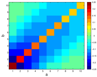
Refer to caption
Figure 13: Illustration of R(a,b)superscript𝑅𝑎𝑏R^{-}(a,b).

From Lemma .3, we can conclude that for any positive integers a,b𝑎𝑏a,b with a+b3𝑎𝑏3a+b\neq 3:

R(1,2)=R(2,1)<R(a,b).superscript𝑅12superscript𝑅21superscript𝑅𝑎𝑏\displaystyle R^{-}(1,2)=R^{-}(2,1)<R^{-}(a,b). (38)

Recall that the pessimistic KG selects:

it=argmaxi{1,,K}R(ait,bit).subscript𝑖𝑡subscriptargmax𝑖1𝐾superscript𝑅superscriptsubscript𝑎𝑖𝑡superscriptsubscript𝑏𝑖𝑡i_{t}=\mathop{\mathrm{arg\,max}{}}_{i\in\{1,\ldots,K\}}R^{-}(a_{i}^{t},b_{i}^{t}).

When starting from the uniform prior with ai0=bi0=1superscriptsubscript𝑎𝑖0superscriptsubscript𝑏𝑖01a_{i}^{0}=b_{i}^{0}=1 for all i{1,K}𝑖1𝐾i\in\{1\ldots,K\}, the corresponding R(ai0,bi0)=R(1,1)>0superscript𝑅superscriptsubscript𝑎𝑖0superscriptsubscript𝑏𝑖0superscript𝑅110R^{-}(a_{i}^{0},b_{i}^{0})=R^{-}(1,1)>0. After obtaining a label for any instance i𝑖i, the Beta parameters for θisubscript𝜃𝑖\theta_{i} will become either (2,1)21(2,1) or (1,2)12(1,2) with R(1,2)=R(2,1)<0superscript𝑅12superscript𝑅210R^{-}(1,2)=R^{-}(2,1)<0. Therefore, for the first K𝐾K stages, the pessimistic KG policy will acquire the label for each instance once. For any instance i𝑖i, we have either aiK=2,biK=1formulae-sequencesuperscriptsubscript𝑎𝑖𝐾2superscriptsubscript𝑏𝑖𝐾1a_{i}^{K}=2,b_{i}^{K}=1 or aiK=1,biK=2formulae-sequencesuperscriptsubscript𝑎𝑖𝐾1superscriptsubscript𝑏𝑖𝐾2a_{i}^{K}=1,b_{i}^{K}=2 at the stage K𝐾K. Then the pessimistic KG policy will select the first instance to label. According to (38), for any tK𝑡𝐾t\geq K, R(a1t,b1t)>R(1,2)=R(2,1)superscript𝑅subscriptsuperscript𝑎𝑡1subscriptsuperscript𝑏𝑡1superscript𝑅12superscript𝑅21R^{-}(a^{t}_{1},b^{t}_{1})>R^{-}(1,2)=R^{-}(2,1). Therefore, the pessimistic KG policy will consistently acquire the label for the first instance. Since the tie will only appear at the stage K𝐾K, the randomized pessimistic KG will also consistently select a single instance to label after K𝐾K stages.

Incorporate Reliability of Heterogeneous Workers

As we discussed in Section 5 in main text, we approximate the posterior so that at any stage for all i,j𝑖𝑗i,j, θisubscript𝜃𝑖\theta_{i} and ρjsubscript𝜌𝑗\rho_{j} will follow Beta distributions. In particular, assuming at the current state θiBeta(ai,bi)similar-tosubscript𝜃𝑖Betasubscript𝑎𝑖subscript𝑏𝑖\theta_{i}\sim\text{Beta}(a_{i},b_{i}) and ρjBeta(cj,dj)similar-tosubscript𝜌𝑗Betasubscript𝑐𝑗subscript𝑑𝑗\rho_{j}\sim\text{Beta}(c_{j},d_{j}), the posterior distribution conditioned on zijsubscript𝑧𝑖𝑗z_{ij} takes the following form:

p(θi,ρj|zij=1)=Pr(zij=1|θi,ρj)Beta(ai,bi)Beta(cj,dj)Pr(zij=1)𝑝subscript𝜃𝑖conditionalsubscript𝜌𝑗subscript𝑧𝑖𝑗1Prsubscript𝑧𝑖𝑗conditional1subscript𝜃𝑖subscript𝜌𝑗Betasubscript𝑎𝑖subscript𝑏𝑖Betasubscript𝑐𝑗subscript𝑑𝑗Prsubscript𝑧𝑖𝑗1\displaystyle p(\theta_{i},\rho_{j}|z_{ij}=1)=\frac{\Pr(z_{ij}=1|\theta_{i},\rho_{j})\text{Beta}(a_{i},b_{i})\text{Beta}(c_{j},d_{j})}{\Pr(z_{ij}=1)}
p(θi,ρj|zij=1)=Pr(zij=1|θi,ρj)Beta(ai,bi)Beta(cj,dj)Pr(zij=1)𝑝subscript𝜃𝑖conditionalsubscript𝜌𝑗subscript𝑧𝑖𝑗1Prsubscript𝑧𝑖𝑗conditional1subscript𝜃𝑖subscript𝜌𝑗Betasubscript𝑎𝑖subscript𝑏𝑖Betasubscript𝑐𝑗subscript𝑑𝑗Prsubscript𝑧𝑖𝑗1\displaystyle p(\theta_{i},\rho_{j}|z_{ij}=-1)=\frac{\Pr(z_{ij}=-1|\theta_{i},\rho_{j})\text{Beta}(a_{i},b_{i})\text{Beta}(c_{j},d_{j})}{\Pr(z_{ij}=-1)}

where the likelihood Pr(zij=z|θi,ρj)Prsubscript𝑧𝑖𝑗conditional𝑧subscript𝜃𝑖subscript𝜌𝑗\Pr(z_{ij}=z|\theta_{i},\rho_{j}) for z=1,1𝑧11z=1,-1 is defined in (18) and (19), i.e.,

Pr(zij=1|θi,ρj)Prsubscript𝑧𝑖𝑗conditional1subscript𝜃𝑖subscript𝜌𝑗\displaystyle\Pr(z_{ij}=1|\theta_{i},\rho_{j}) =\displaystyle= θiρj+(1θi)(1ρj)subscript𝜃𝑖subscript𝜌𝑗1subscript𝜃𝑖1subscript𝜌𝑗\displaystyle\theta_{i}\rho_{j}+(1-\theta_{i})(1-\rho_{j})
Pr(zij=1|θi,ρj)Prsubscript𝑧𝑖𝑗conditional1subscript𝜃𝑖subscript𝜌𝑗\displaystyle\Pr(z_{ij}=-1|\theta_{i},\rho_{j}) =\displaystyle= (1θi)ρj+θi(1ρj)1subscript𝜃𝑖subscript𝜌𝑗subscript𝜃𝑖1subscript𝜌𝑗\displaystyle(1-\theta_{i})\rho_{j}+\theta_{i}(1-\rho_{j})

Also,

Pr(zij=1)Prsubscript𝑧𝑖𝑗1\displaystyle\Pr(z_{ij}=1) =𝔼(Pr(zij=1|θi,ρj))=𝔼(θi)𝔼(ρj)+(1𝔼(θi))(1𝔼(ρj))absent𝔼Prsubscript𝑧𝑖𝑗conditional1subscript𝜃𝑖subscript𝜌𝑗𝔼subscript𝜃𝑖𝔼subscript𝜌𝑗1𝔼subscript𝜃𝑖1𝔼subscript𝜌𝑗\displaystyle=\mathbb{E}(\Pr(z_{ij}=1|\theta_{i},\rho_{j}))=\mathbb{E}(\theta_{i})\mathbb{E}(\rho_{j})+(1-\mathbb{E}(\theta_{i}))(1-\mathbb{E}(\rho_{j}))
=aiai+bicjcj+dj+biai+bidjcj+dj.absentsubscript𝑎𝑖subscript𝑎𝑖subscript𝑏𝑖subscript𝑐𝑗subscript𝑐𝑗subscript𝑑𝑗subscript𝑏𝑖subscript𝑎𝑖subscript𝑏𝑖subscript𝑑𝑗subscript𝑐𝑗subscript𝑑𝑗\displaystyle=\frac{a_{i}}{a_{i}+b_{i}}\frac{c_{j}}{c_{j}+d_{j}}+\frac{b_{i}}{a_{i}+b_{i}}\frac{d_{j}}{c_{j}+d_{j}}.
Pr(zij=1)Prsubscript𝑧𝑖𝑗1\displaystyle\Pr(z_{ij}=-1) =𝔼(Pr(zij=1|θi,ρj))=(1𝔼(θi))𝔼(ρj)+𝔼(θi)(1𝔼(ρj))absent𝔼Prsubscript𝑧𝑖𝑗conditional1subscript𝜃𝑖subscript𝜌𝑗1𝔼subscript𝜃𝑖𝔼subscript𝜌𝑗𝔼subscript𝜃𝑖1𝔼subscript𝜌𝑗\displaystyle=\mathbb{E}(\Pr(z_{ij}=-1|\theta_{i},\rho_{j}))=(1-\mathbb{E}(\theta_{i}))\mathbb{E}(\rho_{j})+\mathbb{E}(\theta_{i})(1-\mathbb{E}(\rho_{j}))
=biai+bicjcj+dj+aiai+bidjcj+dj.absentsubscript𝑏𝑖subscript𝑎𝑖subscript𝑏𝑖subscript𝑐𝑗subscript𝑐𝑗subscript𝑑𝑗subscript𝑎𝑖subscript𝑎𝑖subscript𝑏𝑖subscript𝑑𝑗subscript𝑐𝑗subscript𝑑𝑗\displaystyle=\frac{b_{i}}{a_{i}+b_{i}}\frac{c_{j}}{c_{j}+d_{j}}+\frac{a_{i}}{a_{i}+b_{i}}\frac{d_{j}}{c_{j}+d_{j}}.

The posterior distributions p(θi,pj|zij=z)𝑝subscript𝜃𝑖conditionalsubscript𝑝𝑗subscript𝑧𝑖𝑗𝑧p(\theta_{i},p_{j}|z_{ij}=z) no longer takes the form of the product of Beta distributions on θisubscript𝜃𝑖\theta_{i} and pjsubscript𝑝𝑗p_{j}. Therefore, we use variational approximation by first assuming the conditional independence of θisubscript𝜃𝑖\theta_{i} and ρjsubscript𝜌𝑗\rho_{j}:

p(θi,ρj|zij=z)p(θi|zij=z)p(ρj|zij=z)𝑝subscript𝜃𝑖conditionalsubscript𝜌𝑗subscript𝑧𝑖𝑗𝑧𝑝conditionalsubscript𝜃𝑖subscript𝑧𝑖𝑗𝑧𝑝conditionalsubscript𝜌𝑗subscript𝑧𝑖𝑗𝑧\displaystyle p(\theta_{i},\rho_{j}|z_{ij}=z)\approx p(\theta_{i}|z_{ij}=z)p(\rho_{j}|z_{ij}=z)

In fact, the exact form of marginal distributions can be calculated as follows:

p(θi|zij=1)𝑝conditionalsubscript𝜃𝑖subscript𝑧𝑖𝑗1\displaystyle p(\theta_{i}|z_{ij}=1) =θi𝔼(ρj)+(1θi)(1𝔼(ρj))Pr(zij=1)Beta(ai,bi)absentsubscript𝜃𝑖𝔼subscript𝜌𝑗1subscript𝜃𝑖1𝔼subscript𝜌𝑗Prsubscript𝑧𝑖𝑗1Betasubscript𝑎𝑖subscript𝑏𝑖\displaystyle=\frac{\theta_{i}\mathbb{E}(\rho_{j})+(1-\theta_{i})(1-\mathbb{E}(\rho_{j}))}{\Pr(z_{ij}=1)}\text{Beta}(a_{i},b_{i})
p(ρj|zij=1)𝑝conditionalsubscript𝜌𝑗subscript𝑧𝑖𝑗1\displaystyle p(\rho_{j}|z_{ij}=1) =𝔼(θi)ρj+(1𝔼(θi))(1ρj)Pr(zij=1)Beta(cj,dj)absent𝔼subscript𝜃𝑖subscript𝜌𝑗1𝔼subscript𝜃𝑖1subscript𝜌𝑗Prsubscript𝑧𝑖𝑗1Betasubscript𝑐𝑗subscript𝑑𝑗\displaystyle=\frac{\mathbb{E}(\theta_{i})\rho_{j}+(1-\mathbb{E}(\theta_{i}))(1-\rho_{j})}{\Pr(z_{ij}=1)}\text{Beta}(c_{j},d_{j})
p(θi|zij=1)𝑝conditionalsubscript𝜃𝑖subscript𝑧𝑖𝑗1\displaystyle p(\theta_{i}|z_{ij}=-1) =(1θi)𝔼(ρj)+θi(1𝔼(ρj))Pr(zij=1)Beta(ai,bi)absent1subscript𝜃𝑖𝔼subscript𝜌𝑗subscript𝜃𝑖1𝔼subscript𝜌𝑗Prsubscript𝑧𝑖𝑗1Betasubscript𝑎𝑖subscript𝑏𝑖\displaystyle=\frac{(1-\theta_{i})\mathbb{E}(\rho_{j})+\theta_{i}(1-\mathbb{E}(\rho_{j}))}{\Pr(z_{ij}=-1)}\text{Beta}(a_{i},b_{i})
p(ρj|zij=1)𝑝conditionalsubscript𝜌𝑗subscript𝑧𝑖𝑗1\displaystyle p(\rho_{j}|z_{ij}=-1) =(1𝔼(θi))ρj+𝔼(θi)(1ρj)Pr(zij=1)Beta(cj,dj).absent1𝔼subscript𝜃𝑖subscript𝜌𝑗𝔼subscript𝜃𝑖1subscript𝜌𝑗Prsubscript𝑧𝑖𝑗1Betasubscript𝑐𝑗subscript𝑑𝑗\displaystyle=\frac{(1-\mathbb{E}(\theta_{i}))\rho_{j}+\mathbb{E}(\theta_{i})(1-\rho_{j})}{\Pr(z_{ij}=-1)}\text{Beta}(c_{j},d_{j}).

To approximate the marginal distribution as Beta distribution, we use the moment matching technique. In particular, we approximate p(θi|zij=z)Beta(a~i(z),b~i(z))𝑝conditionalsubscript𝜃𝑖subscript𝑧𝑖𝑗𝑧Betasubscript~𝑎𝑖𝑧subscript~𝑏𝑖𝑧p\left(\theta_{i}|z_{ij}=z\right)\approx\text{Beta}(\tilde{a}_{i}(z),\tilde{b}_{i}(z)) such that

𝔼~z(θi)𝔼p(θi|zij=z)(θi)approaches-limitsubscript~𝔼𝑧subscript𝜃𝑖subscript𝔼𝑝conditionalsubscript𝜃𝑖subscript𝑧𝑖𝑗𝑧subscript𝜃𝑖\displaystyle\widetilde{\mathbb{E}}_{z}(\theta_{i})\doteq\mathbb{E}_{p(\theta_{i}|z_{ij}=z)}(\theta_{i}) =a~i(z)a~i(z)+b~i(z),absentsubscript~𝑎𝑖𝑧subscript~𝑎𝑖𝑧subscript~𝑏𝑖𝑧\displaystyle=\frac{\tilde{a}_{i}(z)}{\tilde{a}_{i}(z)+\tilde{b}_{i}(z)}, (39)
𝔼~z(θi2)𝔼p(θi|zij=z)(θi2)approaches-limitsubscript~𝔼𝑧superscriptsubscript𝜃𝑖2subscript𝔼𝑝conditionalsubscript𝜃𝑖subscript𝑧𝑖𝑗𝑧superscriptsubscript𝜃𝑖2\displaystyle\widetilde{\mathbb{E}}_{z}(\theta_{i}^{2})\doteq\mathbb{E}_{p(\theta_{i}|z_{ij}=z)}(\theta_{i}^{2}) =a~i(z)(a~i(z)+1)(a~i(z)+b~i(z))(a~i(z)+b~i(z)+1),absentsubscript~𝑎𝑖𝑧subscript~𝑎𝑖𝑧1subscript~𝑎𝑖𝑧subscript~𝑏𝑖𝑧subscript~𝑎𝑖𝑧subscript~𝑏𝑖𝑧1\displaystyle=\frac{\tilde{a}_{i}(z)(\tilde{a}_{i}(z)+1)}{(\tilde{a}_{i}(z)+\tilde{b}_{i}(z))(\tilde{a}_{i}(z)+\tilde{b}_{i}(z)+1)}, (40)

where a~i(z)a~i(z)+b~i(z)subscript~𝑎𝑖𝑧subscript~𝑎𝑖𝑧subscript~𝑏𝑖𝑧\frac{\tilde{a}_{i}(z)}{\tilde{a}_{i}(z)+\tilde{b}_{i}(z)} and a~i(z)(a~i(z)+1)(a~i(z)+b~i(z))(a~i(z)+b~i(z)+1)subscript~𝑎𝑖𝑧subscript~𝑎𝑖𝑧1subscript~𝑎𝑖𝑧subscript~𝑏𝑖𝑧subscript~𝑎𝑖𝑧subscript~𝑏𝑖𝑧1\frac{\tilde{a}_{i}(z)(\tilde{a}_{i}(z)+1)}{(\tilde{a}_{i}(z)+\tilde{b}_{i}(z))(\tilde{a}_{i}(z)+\tilde{b}_{i}(z)+1)} are the first and second order moment of Beta(a~i(z),b~i(z))Betasubscript~𝑎𝑖𝑧subscript~𝑏𝑖𝑧\text{Beta}(\tilde{a}_{i}(z),\tilde{b}_{i}(z)). To make (39) and (40) hold, we have:

a~i(z)subscript~𝑎𝑖𝑧\displaystyle\tilde{a}_{i}(z) =𝔼~z(θi)𝔼~z(θi)𝔼~z(θi2)𝔼~z(θi2)(𝔼~z(θi))2,absentsubscript~𝔼𝑧subscript𝜃𝑖subscript~𝔼𝑧subscript𝜃𝑖subscript~𝔼𝑧superscriptsubscript𝜃𝑖2subscript~𝔼𝑧superscriptsubscript𝜃𝑖2superscriptsubscript~𝔼𝑧subscript𝜃𝑖2\displaystyle=\widetilde{\mathbb{E}}_{z}(\theta_{i})\frac{\widetilde{\mathbb{E}}_{z}(\theta_{i})-\widetilde{\mathbb{E}}_{z}(\theta_{i}^{2})}{\widetilde{\mathbb{E}}_{z}(\theta_{i}^{2})-\left(\widetilde{\mathbb{E}}_{z}(\theta_{i})\right)^{2}}, (41)
b~i(z)subscript~𝑏𝑖𝑧\displaystyle\tilde{b}_{i}(z) =(1𝔼~z(θi))𝔼~z(θi)𝔼~z(θi2)𝔼~z(θi2)(𝔼~z(θi))2.absent1subscript~𝔼𝑧subscript𝜃𝑖subscript~𝔼𝑧subscript𝜃𝑖subscript~𝔼𝑧superscriptsubscript𝜃𝑖2subscript~𝔼𝑧superscriptsubscript𝜃𝑖2superscriptsubscript~𝔼𝑧subscript𝜃𝑖2\displaystyle=(1-\widetilde{\mathbb{E}}_{z}(\theta_{i}))\frac{\widetilde{\mathbb{E}}_{z}(\theta_{i})-\widetilde{\mathbb{E}}_{z}(\theta_{i}^{2})}{\widetilde{\mathbb{E}}_{z}(\theta_{i}^{2})-\left(\widetilde{\mathbb{E}}_{z}(\theta_{i})\right)^{2}}. (42)

Similarly, we approximate p(ρj|zij=z)Beta(c~j(z),d~j(z))𝑝conditionalsubscript𝜌𝑗subscript𝑧𝑖𝑗𝑧Betasubscript~𝑐𝑗𝑧subscript~𝑑𝑗𝑧p\left(\rho_{j}|z_{ij}=z\right)\approx\text{Beta}(\tilde{c}_{j}(z),\tilde{d}_{j}(z)), such that

𝔼~z(ρj)𝔼p(ρj|zij=z)(ρj)approaches-limitsubscript~𝔼𝑧subscript𝜌𝑗subscript𝔼𝑝conditionalsubscript𝜌𝑗subscript𝑧𝑖𝑗𝑧subscript𝜌𝑗\displaystyle\widetilde{\mathbb{E}}_{z}(\rho_{j})\doteq\mathbb{E}_{p(\rho_{j}|z_{ij}=z)}(\rho_{j}) =c~j(z)c~j(z)+d~j(z),absentsubscript~𝑐𝑗𝑧subscript~𝑐𝑗𝑧subscript~𝑑𝑗𝑧\displaystyle=\frac{\tilde{c}_{j}(z)}{\tilde{c}_{j}(z)+\tilde{d}_{j}(z)}, (43)
𝔼~z(ρj2)𝔼p(ρj|zij=z)(ρj2)approaches-limitsubscript~𝔼𝑧superscriptsubscript𝜌𝑗2subscript𝔼𝑝conditionalsubscript𝜌𝑗subscript𝑧𝑖𝑗𝑧superscriptsubscript𝜌𝑗2\displaystyle\widetilde{\mathbb{E}}_{z}(\rho_{j}^{2})\doteq\mathbb{E}_{p(\rho_{j}|z_{ij}=z)}(\rho_{j}^{2}) =c~j(z)(c~j(z)+1)(c~j(z)+d~j(z))(c~j(z)+d~j(z)+1),absentsubscript~𝑐𝑗𝑧subscript~𝑐𝑗𝑧1subscript~𝑐𝑗𝑧subscript~𝑑𝑗𝑧subscript~𝑐𝑗𝑧subscript~𝑑𝑗𝑧1\displaystyle=\frac{\tilde{c}_{j}(z)(\tilde{c}_{j}(z)+1)}{(\tilde{c}_{j}(z)+\tilde{d}_{j}(z))(\tilde{c}_{j}(z)+\tilde{d}_{j}(z)+1)}, (44)

where c~j(z)c~j(z)+d~j(z)subscript~𝑐𝑗𝑧subscript~𝑐𝑗𝑧subscript~𝑑𝑗𝑧\frac{\tilde{c}_{j}(z)}{\tilde{c}_{j}(z)+\tilde{d}_{j}(z)} and c~j(z)(c~j(z)+1)(c~j(z)+d~j(z))(c~j(z)+d~j(z)+1)subscript~𝑐𝑗𝑧subscript~𝑐𝑗𝑧1subscript~𝑐𝑗𝑧subscript~𝑑𝑗𝑧subscript~𝑐𝑗𝑧subscript~𝑑𝑗𝑧1\frac{\tilde{c}_{j}(z)(\tilde{c}_{j}(z)+1)}{(\tilde{c}_{j}(z)+\tilde{d}_{j}(z))(\tilde{c}_{j}(z)+\tilde{d}_{j}(z)+1)} are the first and second order moment of Beta(c~j(z),d~j(z))Betasubscript~𝑐𝑗𝑧subscript~𝑑𝑗𝑧\text{Beta}(\tilde{c}_{j}(z),\tilde{d}_{j}(z)). To make (39) and (40) hold, we have:

c~j(z)subscript~𝑐𝑗𝑧\displaystyle\tilde{c}_{j}(z) =𝔼~z(ρj)𝔼~z(ρj)𝔼~z(ρj2)𝔼~z(ρj2)(𝔼~z(ρj))2,absentsubscript~𝔼𝑧subscript𝜌𝑗subscript~𝔼𝑧subscript𝜌𝑗subscript~𝔼𝑧superscriptsubscript𝜌𝑗2subscript~𝔼𝑧superscriptsubscript𝜌𝑗2superscriptsubscript~𝔼𝑧subscript𝜌𝑗2\displaystyle=\widetilde{\mathbb{E}}_{z}(\rho_{j})\frac{\widetilde{\mathbb{E}}_{z}(\rho_{j})-\widetilde{\mathbb{E}}_{z}(\rho_{j}^{2})}{\widetilde{\mathbb{E}}_{z}(\rho_{j}^{2})-\left(\widetilde{\mathbb{E}}_{z}(\rho_{j})\right)^{2}}, (45)
d~j(z)subscript~𝑑𝑗𝑧\displaystyle\tilde{d}_{j}(z) =(1𝔼~z(ρj))𝔼~z(ρj)𝔼~z(ρj2)𝔼~z(ρj2)(𝔼~z(ρj))2.absent1subscript~𝔼𝑧subscript𝜌𝑗subscript~𝔼𝑧subscript𝜌𝑗subscript~𝔼𝑧superscriptsubscript𝜌𝑗2subscript~𝔼𝑧superscriptsubscript𝜌𝑗2superscriptsubscript~𝔼𝑧subscript𝜌𝑗2\displaystyle=(1-\widetilde{\mathbb{E}}_{z}(\rho_{j}))\frac{\widetilde{\mathbb{E}}_{z}(\rho_{j})-\widetilde{\mathbb{E}}_{z}(\rho_{j}^{2})}{\widetilde{\mathbb{E}}_{z}(\rho_{j}^{2})-\left(\widetilde{\mathbb{E}}_{z}(\rho_{j})\right)^{2}}. (46)

Furthermore, we can compute the exact values for 𝔼~z(θi)subscript~𝔼𝑧subscript𝜃𝑖\widetilde{\mathbb{E}}_{z}(\theta_{i}), 𝔼~z(θi2)subscript~𝔼𝑧superscriptsubscript𝜃𝑖2\widetilde{\mathbb{E}}_{z}(\theta_{i}^{2}), 𝔼~z(ρj)subscript~𝔼𝑧subscript𝜌𝑗\widetilde{\mathbb{E}}_{z}(\rho_{j}) and 𝔼~z(ρj2)subscript~𝔼𝑧superscriptsubscript𝜌𝑗2\widetilde{\mathbb{E}}_{z}(\rho_{j}^{2}) as follows.

𝔼~1(θi)subscript~𝔼1subscript𝜃𝑖\displaystyle\widetilde{\mathbb{E}}_{1}(\theta_{i}) =𝔼(θi2)𝔼(ρj)+(𝔼(θi)𝔼(θi2))(1𝔼(ρj))p(zij=1)=ai((ai+1)cj+bidj)(ai+bi+1)(aicj+bidj);absent𝔼superscriptsubscript𝜃𝑖2𝔼subscript𝜌𝑗𝔼subscript𝜃𝑖𝔼superscriptsubscript𝜃𝑖21𝔼subscript𝜌𝑗𝑝subscript𝑧𝑖𝑗1subscript𝑎𝑖subscript𝑎𝑖1subscript𝑐𝑗subscript𝑏𝑖subscript𝑑𝑗subscript𝑎𝑖subscript𝑏𝑖1subscript𝑎𝑖subscript𝑐𝑗subscript𝑏𝑖subscript𝑑𝑗\displaystyle=\frac{\mathbb{E}(\theta_{i}^{2})\mathbb{E}(\rho_{j})+(\mathbb{E}(\theta_{i})-\mathbb{E}(\theta_{i}^{2}))(1-\mathbb{E}(\rho_{j}))}{p(z_{ij}=1)}=\frac{a_{i}((a_{i}+1)c_{j}+b_{i}d_{j})}{(a_{i}+b_{i}+1)(a_{i}c_{j}+b_{i}d_{j})};
𝔼~1(θi2)subscript~𝔼1superscriptsubscript𝜃𝑖2\displaystyle\widetilde{\mathbb{E}}_{1}(\theta_{i}^{2}) =𝔼(θi3)𝔼(ρj)+(𝔼(θi2)𝔼(θi3))(1𝔼(ρj))p(zij=1)=ai(ai+1)((ai+2)cj+bidj)(ai+bi+1)(ai+bi+2)(aicj+bidj);absent𝔼superscriptsubscript𝜃𝑖3𝔼subscript𝜌𝑗𝔼superscriptsubscript𝜃𝑖2𝔼superscriptsubscript𝜃𝑖31𝔼subscript𝜌𝑗𝑝subscript𝑧𝑖𝑗1subscript𝑎𝑖subscript𝑎𝑖1subscript𝑎𝑖2subscript𝑐𝑗subscript𝑏𝑖subscript𝑑𝑗subscript𝑎𝑖subscript𝑏𝑖1subscript𝑎𝑖subscript𝑏𝑖2subscript𝑎𝑖subscript𝑐𝑗subscript𝑏𝑖subscript𝑑𝑗\displaystyle=\frac{\mathbb{E}(\theta_{i}^{3})\mathbb{E}(\rho_{j})+(\mathbb{E}(\theta_{i}^{2})-\mathbb{E}(\theta_{i}^{3}))(1-\mathbb{E}(\rho_{j}))}{p(z_{ij}=1)}=\frac{a_{i}(a_{i}+1)((a_{i}+2)c_{j}+b_{i}d_{j})}{(a_{i}+b_{i}+1)(a_{i}+b_{i}+2)(a_{i}c_{j}+b_{i}d_{j})};
𝔼~1(θi)subscript~𝔼1subscript𝜃𝑖\displaystyle\widetilde{\mathbb{E}}_{-1}(\theta_{i}) =(𝔼(θi)𝔼(θi2))𝔼(ρj)+𝔼(θi2)(1𝔼(ρj))p(zij=1)=ai(bicj+(ai+1)dj)(ai+bi+1)(bicj+aidj);absent𝔼subscript𝜃𝑖𝔼superscriptsubscript𝜃𝑖2𝔼subscript𝜌𝑗𝔼superscriptsubscript𝜃𝑖21𝔼subscript𝜌𝑗𝑝subscript𝑧𝑖𝑗1subscript𝑎𝑖subscript𝑏𝑖subscript𝑐𝑗subscript𝑎𝑖1subscript𝑑𝑗subscript𝑎𝑖subscript𝑏𝑖1subscript𝑏𝑖subscript𝑐𝑗subscript𝑎𝑖subscript𝑑𝑗\displaystyle=\frac{(\mathbb{E}(\theta_{i})-\mathbb{E}(\theta_{i}^{2}))\mathbb{E}(\rho_{j})+\mathbb{E}(\theta_{i}^{2})(1-\mathbb{E}(\rho_{j}))}{p(z_{ij}=-1)}=\frac{a_{i}(b_{i}c_{j}+(a_{i}+1)d_{j})}{(a_{i}+b_{i}+1)(b_{i}c_{j}+a_{i}d_{j})};
𝔼~1(θi2)subscript~𝔼1superscriptsubscript𝜃𝑖2\displaystyle\widetilde{\mathbb{E}}_{-1}(\theta_{i}^{2}) =(𝔼(θi2)𝔼(θi3))𝔼(ρj)+𝔼(θi3)(1𝔼(ρj))p(zij=1)=ai(ai+1)(bicj+(ai+2)dj)(ai+bi+1)(ai+bi+2)(bicj+aidj);absent𝔼superscriptsubscript𝜃𝑖2𝔼superscriptsubscript𝜃𝑖3𝔼subscript𝜌𝑗𝔼superscriptsubscript𝜃𝑖31𝔼subscript𝜌𝑗𝑝subscript𝑧𝑖𝑗1subscript𝑎𝑖subscript𝑎𝑖1subscript𝑏𝑖subscript𝑐𝑗subscript𝑎𝑖2subscript𝑑𝑗subscript𝑎𝑖subscript𝑏𝑖1subscript𝑎𝑖subscript𝑏𝑖2subscript𝑏𝑖subscript𝑐𝑗subscript𝑎𝑖subscript𝑑𝑗\displaystyle=\frac{(\mathbb{E}(\theta_{i}^{2})-\mathbb{E}(\theta_{i}^{3}))\mathbb{E}(\rho_{j})+\mathbb{E}(\theta_{i}^{3})(1-\mathbb{E}(\rho_{j}))}{p(z_{ij}=-1)}=\frac{a_{i}(a_{i}+1)(b_{i}c_{j}+(a_{i}+2)d_{j})}{(a_{i}+b_{i}+1)(a_{i}+b_{i}+2)(b_{i}c_{j}+a_{i}d_{j})};
𝔼~1(ρj)subscript~𝔼1subscript𝜌𝑗\displaystyle\widetilde{\mathbb{E}}_{1}(\rho_{j}) =𝔼(θi)𝔼(ρj2)+(1𝔼(θi))(𝔼(ρj)𝔼(ρj2))p(zij=1)=cj(ai(cj+1)+bidj)(cj+dj+1)(aicj+bidj);absent𝔼subscript𝜃𝑖𝔼superscriptsubscript𝜌𝑗21𝔼subscript𝜃𝑖𝔼subscript𝜌𝑗𝔼superscriptsubscript𝜌𝑗2𝑝subscript𝑧𝑖𝑗1subscript𝑐𝑗subscript𝑎𝑖subscript𝑐𝑗1subscript𝑏𝑖subscript𝑑𝑗subscript𝑐𝑗subscript𝑑𝑗1subscript𝑎𝑖subscript𝑐𝑗subscript𝑏𝑖subscript𝑑𝑗\displaystyle=\frac{\mathbb{E}(\theta_{i})\mathbb{E}(\rho_{j}^{2})+(1-\mathbb{E}(\theta_{i}))(\mathbb{E}(\rho_{j})-\mathbb{E}(\rho_{j}^{2}))}{p(z_{ij}=1)}=\frac{c_{j}(a_{i}(c_{j}+1)+b_{i}d_{j})}{(c_{j}+d_{j}+1)(a_{i}c_{j}+b_{i}d_{j})};
𝔼~1(ρj2)subscript~𝔼1superscriptsubscript𝜌𝑗2\displaystyle\widetilde{\mathbb{E}}_{1}(\rho_{j}^{2}) =𝔼(θi)𝔼(ρj3)+(1𝔼(θi))(𝔼(ρj2)𝔼(ρj3))p(zij=1)=cj(cj+1)(ai(cj+2)+bidj)(cj+dj+1)(cj+dj+2)(aicj+bidj);absent𝔼subscript𝜃𝑖𝔼superscriptsubscript𝜌𝑗31𝔼subscript𝜃𝑖𝔼superscriptsubscript𝜌𝑗2𝔼superscriptsubscript𝜌𝑗3𝑝subscript𝑧𝑖𝑗1subscript𝑐𝑗subscript𝑐𝑗1subscript𝑎𝑖subscript𝑐𝑗2subscript𝑏𝑖subscript𝑑𝑗subscript𝑐𝑗subscript𝑑𝑗1subscript𝑐𝑗subscript𝑑𝑗2subscript𝑎𝑖subscript𝑐𝑗subscript𝑏𝑖subscript𝑑𝑗\displaystyle=\frac{\mathbb{E}(\theta_{i})\mathbb{E}(\rho_{j}^{3})+(1-\mathbb{E}(\theta_{i}))(\mathbb{E}(\rho_{j}^{2})-\mathbb{E}(\rho_{j}^{3}))}{p(z_{ij}=1)}=\frac{c_{j}(c_{j}+1)(a_{i}(c_{j}+2)+b_{i}d_{j})}{(c_{j}+d_{j}+1)(c_{j}+d_{j}+2)(a_{i}c_{j}+b_{i}d_{j})};
𝔼~1(ρj)subscript~𝔼1subscript𝜌𝑗\displaystyle\widetilde{\mathbb{E}}_{{-1}}(\rho_{j}) =(1𝔼(θi))𝔼(ρj2)+𝔼(θi)(𝔼(ρj)𝔼(ρj2))p(zij=1)=cj(bi(cj+1)+aidj)(cj+dj+1)(bicj+aidj);absent1𝔼subscript𝜃𝑖𝔼superscriptsubscript𝜌𝑗2𝔼subscript𝜃𝑖𝔼subscript𝜌𝑗𝔼superscriptsubscript𝜌𝑗2𝑝subscript𝑧𝑖𝑗1subscript𝑐𝑗subscript𝑏𝑖subscript𝑐𝑗1subscript𝑎𝑖subscript𝑑𝑗subscript𝑐𝑗subscript𝑑𝑗1subscript𝑏𝑖subscript𝑐𝑗subscript𝑎𝑖subscript𝑑𝑗\displaystyle=\frac{(1-\mathbb{E}(\theta_{i}))\mathbb{E}(\rho_{j}^{2})+\mathbb{E}(\theta_{i})(\mathbb{E}(\rho_{j})-\mathbb{E}(\rho_{j}^{2}))}{p(z_{ij}=-1)}=\frac{c_{j}(b_{i}(c_{j}+1)+a_{i}d_{j})}{(c_{j}+d_{j}+1)(b_{i}c_{j}+a_{i}d_{j})};
𝔼~1(ρj2)subscript~𝔼1superscriptsubscript𝜌𝑗2\displaystyle\widetilde{\mathbb{E}}_{-1}(\rho_{j}^{2}) =(1𝔼(θi))𝔼(ρj3)+𝔼(θi)(𝔼(ρj2)𝔼(ρj3))p(zij=1)=cj(cj+1)(bi(cj+2)+aidj)(cj+dj+1)(cj+dj+2)(bicj+aidj).absent1𝔼subscript𝜃𝑖𝔼superscriptsubscript𝜌𝑗3𝔼subscript𝜃𝑖𝔼superscriptsubscript𝜌𝑗2𝔼superscriptsubscript𝜌𝑗3𝑝subscript𝑧𝑖𝑗1subscript𝑐𝑗subscript𝑐𝑗1subscript𝑏𝑖subscript𝑐𝑗2subscript𝑎𝑖subscript𝑑𝑗subscript𝑐𝑗subscript𝑑𝑗1subscript𝑐𝑗subscript𝑑𝑗2subscript𝑏𝑖subscript𝑐𝑗subscript𝑎𝑖subscript𝑑𝑗\displaystyle=\frac{(1-\mathbb{E}(\theta_{i}))\mathbb{E}(\rho_{j}^{3})+\mathbb{E}(\theta_{i})(\mathbb{E}(\rho_{j}^{2})-\mathbb{E}(\rho_{j}^{3}))}{p(z_{ij}=-1)}=\frac{c_{j}(c_{j}+1)(b_{i}(c_{j}+2)+a_{i}d_{j})}{(c_{j}+d_{j}+1)(c_{j}+d_{j}+2)(b_{i}c_{j}+a_{i}d_{j})}.

Assuming that at a certain stage, θisubscript𝜃𝑖\theta_{i} follows a Beta posterior Beta(ai,bi)Betasubscript𝑎𝑖subscript𝑏𝑖\text{Beta}(a_{i},b_{i}) and ρjsubscript𝜌𝑗\rho_{j} follows a Beta posterior Beta(cj,dj)Betasubscript𝑐𝑗subscript𝑑𝑗\text{Beta}(c_{j},d_{j}), the reward of getting positive and negative labels for the i𝑖i-th instance from the j𝑗j-th worker are:

R1(ai,bi,cj,dj)subscript𝑅1subscript𝑎𝑖subscript𝑏𝑖subscript𝑐𝑗subscript𝑑𝑗\displaystyle R_{1}(a_{i},b_{i},c_{j},d_{j}) =h(I(a~i(z=1),b~i(z=1)))h(I(ai,bi))absent𝐼subscript~𝑎𝑖𝑧1subscript~𝑏𝑖𝑧1𝐼subscript𝑎𝑖subscript𝑏𝑖\displaystyle=h(I(\tilde{a}_{i}(z=1),\tilde{b}_{i}(z=1)))-h(I(a_{i},b_{i})) (47)
R2(ai,bi,cj,dj)subscript𝑅2subscript𝑎𝑖subscript𝑏𝑖subscript𝑐𝑗subscript𝑑𝑗\displaystyle R_{2}(a_{i},b_{i},c_{j},d_{j}) =h(I(a~i(z=1),b~i(z=1)))h(I(ai,bi)),absent𝐼subscript~𝑎𝑖𝑧1subscript~𝑏𝑖𝑧1𝐼subscript𝑎𝑖subscript𝑏𝑖\displaystyle=h(I(\tilde{a}_{i}(z=-1),\tilde{b}_{i}(z=-1)))-h(I(a_{i},b_{i})), (48)

where a~i(z=±1)subscript~𝑎𝑖𝑧plus-or-minus1\tilde{a}_{i}(z=\pm 1) and b~i(z=±1)subscript~𝑏𝑖𝑧plus-or-minus1\tilde{b}_{i}(z=\pm 1) are defined in (41) and (42), which further depend on cjsubscript𝑐𝑗c_{j} and djsubscript𝑑𝑗d_{j} through 𝔼~z(θi)subscript~𝔼𝑧subscript𝜃𝑖\widetilde{\mathbb{E}}_{z}(\theta_{i}) and 𝔼~z(θi2)subscript~𝔼𝑧superscriptsubscript𝜃𝑖2\widetilde{\mathbb{E}}_{z}(\theta_{i}^{2}). With the reward in place, we can directly apply the Opt-KG policy in the heterogeneous worker setting.

Extensions

Utilizing Contextual Information

When each instance is associated with a p𝑝p-dimensional feature vector 𝐱ipsubscript𝐱𝑖superscript𝑝\mathbf{x}_{i}\in\mathbb{R}^{p}, we incorporate the feature information in our budget allocation problem by assuming:

θi=σ(𝐰,𝐱i)11+exp{𝐰,𝐱i},subscript𝜃𝑖𝜎𝐰subscript𝐱𝑖approaches-limit11𝐰subscript𝐱𝑖\theta_{i}=\sigma(\langle\mathbf{w},\mathbf{x}_{i}\rangle)\doteq\frac{1}{1+\exp\{-\langle\mathbf{w},\mathbf{x}_{i}\rangle\}}, (49)

where σ(x)=11+exp{x}𝜎𝑥11𝑥\sigma(x)=\frac{1}{1+\exp\{-x\}} is the sigmoid function and 𝐰𝐰\mathbf{w} is assumed to be drawn from a Gaussian prior N(𝝁0,𝚺0)𝑁subscript𝝁0subscript𝚺0N(\bm{\mu}_{0},\bm{\Sigma}_{0}). At the t𝑡t-th stage with the state St=(𝝁t,𝚺t)superscript𝑆𝑡subscript𝝁𝑡subscript𝚺𝑡S^{t}=(\bm{\mu}_{t},\bm{\Sigma}_{t}) and 𝐰(𝝁t,𝚺t)similar-to𝐰subscript𝝁𝑡subscript𝚺𝑡\mathbf{w}\sim(\bm{\mu}_{t},\bm{\Sigma}_{t}), the decision maker chooses the itsubscript𝑖𝑡i_{t}-th instance to be labeled and observes the label yit{1,1}subscript𝑦subscript𝑖𝑡11y_{i_{t}}\in\{-1,1\}. The posterior distribution p(𝐰|yit,St)p(yit|𝐰)p(𝐰|St)proportional-to𝑝conditional𝐰subscript𝑦subscript𝑖𝑡superscript𝑆𝑡𝑝conditionalsubscript𝑦subscript𝑖𝑡𝐰𝑝conditional𝐰superscript𝑆𝑡p(\mathbf{w}|y_{i_{t}},S^{t})\propto p(y_{i_{t}}|\mathbf{w})p(\mathbf{w}|S^{t}) has the following log-likelihood:

lnp(𝐰|yit,St)=lnp(yit|𝐰)+lnp(𝐰|St)+const𝑝conditional𝐰subscript𝑦subscript𝑖𝑡superscript𝑆𝑡𝑝conditionalsubscript𝑦subscript𝑖𝑡𝐰𝑝conditional𝐰superscript𝑆𝑡const\displaystyle\ln p(\mathbf{w}|y_{i_{t}},S^{t})=\ln p(y_{i_{t}}|\mathbf{w})+\ln p(\mathbf{w}|S^{t})+\text{const}
=\displaystyle= 𝟏(yit=1)lnσ(𝐰,𝐱it)+𝟏(yit=1)ln(1σ(𝐰,𝐱it))12(𝐰𝝁t)𝛀t(𝐰𝝁t)+const,1subscript𝑦subscript𝑖𝑡1𝜎𝐰subscript𝐱subscript𝑖𝑡1subscript𝑦subscript𝑖𝑡11𝜎𝐰subscript𝐱subscript𝑖𝑡12superscript𝐰subscript𝝁𝑡subscript𝛀𝑡𝐰subscript𝝁𝑡const\displaystyle\mathbf{1}(y_{i_{t}}=1)\ln\sigma(\langle\mathbf{w},\mathbf{x}_{i_{t}}\rangle)+\mathbf{1}(y_{i_{t}}=-1)\ln\left(1-\sigma(\langle\mathbf{w},\mathbf{x}_{i_{t}}\rangle)\right)-\frac{1}{2}(\mathbf{w}-\bm{\mu}_{t})^{\prime}\bm{\Omega}_{t}(\mathbf{w}-\bm{\mu}_{t})+\text{const},

where 𝛀t=(𝚺t)1subscript𝛀𝑡superscriptsubscript𝚺𝑡1\bm{\Omega}_{t}=(\bm{\Sigma}_{t})^{-1} is the precision matrix. To approximate p(𝐰|yit,𝝁t,𝚺t)𝑝conditional𝐰subscript𝑦subscript𝑖𝑡subscript𝝁𝑡subscript𝚺𝑡p(\mathbf{w}|y_{i_{t}},\bm{\mu}_{t},\bm{\Sigma}_{t}) by a Gaussian distribution N(𝝁t+1,𝚺t+1)𝑁subscript𝝁𝑡1subscript𝚺𝑡1N(\bm{\mu}_{t+1},\bm{\Sigma}_{t+1}), we use the Laplace method (see Chapter 4.4 in [4]). In particular, the mean of the posterior Gaussian is the MAP (maximum a posteriori) estimator of 𝐰𝐰\mathbf{w}:

μt+1=argmax𝐰lnp(𝐰|yit,St),subscript𝜇𝑡1subscriptargmax𝐰𝑝conditional𝐰subscript𝑦subscript𝑖𝑡superscript𝑆𝑡\mu_{t+1}=\mathop{\mathrm{arg\,max}{}}_{\mathbf{w}}\ln p(\mathbf{w}|y_{i_{t}},S^{t}), (50)

which can be computed by any numerical optimization method (e.g., Newton’s method). The precision matrix takes the following form,

𝛀t+1subscript𝛀𝑡1\displaystyle\bm{\Omega}_{t+1} =2lnp(𝐰|yit,St)|𝐰=𝝁t+1=𝛀t+σ(𝝁t+1𝐱it+1)(1σ(𝝁t+1𝐱it+1))𝐱it+1𝐱it+1.absentevaluated-atsuperscript2𝑝conditional𝐰subscript𝑦subscript𝑖𝑡superscript𝑆𝑡𝐰subscript𝝁𝑡1subscript𝛀𝑡𝜎superscriptsubscript𝝁𝑡1subscript𝐱subscript𝑖𝑡11𝜎superscriptsubscript𝝁𝑡1subscript𝐱subscript𝑖𝑡1subscript𝐱subscript𝑖𝑡1superscriptsubscript𝐱subscript𝑖𝑡1\displaystyle=-\nabla^{2}\ln p(\mathbf{w}|y_{i_{t}},S^{t})\big{|}_{\mathbf{w}=\bm{\mu}_{t+1}}=\bm{\Omega}_{t}+\sigma(\bm{\mu}_{t+1}^{\prime}\mathbf{x}_{i_{t+1}})(1-\sigma(\bm{\mu}_{t+1}^{\prime}\mathbf{x}_{i_{t+1}}))\mathbf{x}_{i_{t+1}}\mathbf{x}_{i_{t+1}}^{\prime}.

By Sherman-Morrison formula, the covariance matrix can be computed as,

𝚺t+1=(𝛀t+1)1=𝚺tσ(𝝁t+1𝐱it)(1σ(𝝁t+1𝐱it))1+σ(𝝁t+1𝐱it)(1σ(𝝁t+1𝐱it))𝐱it𝚺t𝐱it𝚺t𝐱it+1𝐱it𝚺t.subscript𝚺𝑡1superscriptsubscript𝛀𝑡11subscript𝚺𝑡𝜎superscriptsubscript𝝁𝑡1subscript𝐱subscript𝑖𝑡1𝜎subscript𝝁𝑡1subscript𝐱subscript𝑖𝑡1𝜎superscriptsubscript𝝁𝑡1subscript𝐱subscript𝑖𝑡1𝜎superscriptsubscript𝝁𝑡1subscript𝐱subscript𝑖𝑡superscriptsubscript𝐱subscript𝑖𝑡subscript𝚺𝑡subscript𝐱subscript𝑖𝑡subscript𝚺𝑡subscript𝐱subscript𝑖𝑡1superscriptsubscript𝐱subscript𝑖𝑡subscript𝚺𝑡\displaystyle\bm{\Sigma}_{t+1}=(\bm{\Omega}_{t+1})^{-1}=\bm{\Sigma}_{t}-\frac{\sigma(\bm{\mu}_{t+1}^{\prime}\mathbf{x}_{i_{t}})(1-\sigma(\bm{\mu}_{t+1}\mathbf{x}_{i_{t}}))}{1+\sigma(\bm{\mu}_{t+1}^{\prime}\mathbf{x}_{i_{t}})(1-\sigma(\bm{\mu}_{t+1}^{\prime}\mathbf{x}_{i_{t}}))\mathbf{x}_{i_{t}}^{\prime}\bm{\Sigma}_{t}\mathbf{x}_{i_{t}}}\bm{\Sigma}_{t}\mathbf{x}_{i_{t+1}}\mathbf{x}_{i_{t}}^{\prime}\bm{\Sigma}_{t}.

We also calculate the transition probability of yit=1subscript𝑦subscript𝑖𝑡1y_{i_{t}}=1 and yit=1subscript𝑦subscript𝑖𝑡1y_{i_{t}}=-1 using the technique from Bayesian logistic regression (see Chapter 4.5 in [4]):

Pr(yit=1|St,it)=p(yit=1|𝐰)p(𝐰|St)d𝐰=σ(𝐰𝐱i)p(𝐰|St)d𝐰σ(μiκ(si2)),Prsubscript𝑦subscript𝑖𝑡conditional1superscript𝑆𝑡subscript𝑖𝑡𝑝subscript𝑦subscript𝑖𝑡conditional1𝐰𝑝conditional𝐰superscript𝑆𝑡differential-d𝐰𝜎superscript𝐰subscript𝐱𝑖𝑝conditional𝐰superscript𝑆𝑡differential-d𝐰𝜎subscript𝜇𝑖𝜅superscriptsubscript𝑠𝑖2\displaystyle\Pr(y_{i_{t}}=1|S^{t},i_{t})=\int p(y_{i_{t}}=1|\mathbf{w})p(\mathbf{w}|S^{t})\mathrm{d}\mathbf{w}=\int\sigma(\mathbf{w}^{\prime}\mathbf{x}_{i})p(\mathbf{w}|S^{t})\mathrm{d}\mathbf{w}\approx\sigma(\mu_{i}\kappa(s_{i}^{2})),

where κ(si2)=(1+πsi2/8)1/2𝜅superscriptsubscript𝑠𝑖2superscript1𝜋superscriptsubscript𝑠𝑖2812\kappa(s_{i}^{2})=(1+\pi s_{i}^{2}/8)^{-1/2} and μi=𝝁t,𝐱isubscript𝜇𝑖subscript𝝁𝑡subscript𝐱𝑖\mu_{i}=\langle\bm{\mu}_{t},\mathbf{x}_{i}\rangle and si2=𝐱i𝚺t𝐱isuperscriptsubscript𝑠𝑖2superscriptsubscript𝐱𝑖subscript𝚺𝑡subscript𝐱𝑖s_{i}^{2}=\mathbf{x}_{i}^{\prime}\bm{\Sigma}_{t}\mathbf{x}_{i}.

To calculate the reward function, in addition to the transition probability, we also need to compute:

Pitsuperscriptsubscript𝑃𝑖𝑡\displaystyle P_{i}^{t} =Pr(θi0.5|t)absentPrsubscript𝜃𝑖conditional0.5subscript𝑡\displaystyle=\Pr(\theta_{i}\geq 0.5|\mathcal{F}_{t})
=Pr(11+exp{𝐰t𝐱i}0.5|𝐰tN(𝝁t,𝚺t))absentPr11subscriptsuperscript𝐰𝑡subscript𝐱𝑖conditional0.5subscript𝐰𝑡similar-to𝑁subscript𝝁𝑡subscript𝚺𝑡\displaystyle=\Pr\left(\frac{1}{1+\exp\{-\mathbf{w}^{\prime}_{t}\mathbf{x}_{i}\}}\geq 0.5\Big{|}\mathbf{w}_{t}\sim N(\bm{\mu}_{t},\bm{\Sigma}_{t})\right)
=Pr(𝐰t𝐱i0|𝐰tN(𝝁t,𝚺t))absentPrsubscriptsuperscript𝐰𝑡subscript𝐱𝑖conditional0subscript𝐰𝑡similar-to𝑁subscript𝝁𝑡subscript𝚺𝑡\displaystyle=\Pr(\mathbf{w}^{\prime}_{t}\mathbf{x}_{i}\geq 0|\mathbf{w}_{t}\sim N(\bm{\mu}_{t},\bm{\Sigma}_{t}))
=0(𝐰δ(c𝐰,𝐱i)N(𝐰|𝝁t,𝚺t)d𝐰)dc,absentsuperscriptsubscript0subscript𝐰𝛿𝑐𝐰subscript𝐱𝑖𝑁conditional𝐰subscript𝝁𝑡subscript𝚺𝑡differential-d𝐰differential-d𝑐\displaystyle=\int_{0}^{\infty}\left(\int_{\mathbf{w}}\delta(c-\langle\mathbf{w},\mathbf{x}_{i}\rangle)N(\mathbf{w}|\bm{\mu}_{t},\bm{\Sigma}_{t})\mathrm{d}\mathbf{w}\right)\mathrm{d}c,

where δ()𝛿\delta(\cdot) is the Dirac delta function. Let

p(c)=𝐰δ(c𝐰,𝐱i)N(𝐰|𝝁t,𝚺t)d𝐰.𝑝𝑐subscript𝐰𝛿𝑐𝐰subscript𝐱𝑖𝑁conditional𝐰subscript𝝁𝑡subscript𝚺𝑡differential-d𝐰\displaystyle p(c)=\int_{\mathbf{w}}\delta(c-\langle\mathbf{w},\mathbf{x}_{i}\rangle)N(\mathbf{w}|\bm{\mu}_{t},\bm{\Sigma}_{t})\mathrm{d}\mathbf{w}.

Since the marginal of a Gaussian distribution is still a Gaussian, p(c)𝑝𝑐p(c) is a univariate-Gaussian distribution with the mean and variance:

μisubscript𝜇𝑖\displaystyle\mu_{i} =\displaystyle= 𝔼(c)=𝔼(𝐰),𝐱i=𝝁t,𝐱i𝔼𝑐𝔼𝐰subscript𝐱𝑖subscript𝝁𝑡subscript𝐱𝑖\displaystyle\mathbb{E}(c)=\langle\mathbb{E}(\mathbf{w}),\mathbf{x}_{i}\rangle=\langle\bm{\mu}_{t},\mathbf{x}_{i}\rangle
si2superscriptsubscript𝑠𝑖2\displaystyle s_{i}^{2} =\displaystyle= Var(c)=(𝐱i)Cov(𝐰,𝐰)𝐱i=(𝐱i)𝚺t𝐱i.Var𝑐superscriptsubscript𝐱𝑖Cov𝐰𝐰subscript𝐱𝑖superscriptsubscript𝐱𝑖subscript𝚺𝑡subscript𝐱𝑖\displaystyle\text{Var}(c)=(\mathbf{x}_{i})^{\prime}\text{Cov}(\mathbf{w},\mathbf{w})\mathbf{x}_{i}=(\mathbf{x}_{i})^{\prime}\bm{\Sigma}_{t}\mathbf{x}_{i}.

Therefore, we have:

Pit=0p(c)dc=1Φ(μisi),superscriptsubscript𝑃𝑖𝑡superscriptsubscript0𝑝𝑐differential-d𝑐1Φsubscript𝜇𝑖subscript𝑠𝑖\displaystyle P_{i}^{t}=\int_{0}^{\infty}p(c)\mathrm{d}c=1-\Phi\left(-\frac{\mu_{i}}{s_{i}}\right), (51)

where Φ()Φ\Phi(\cdot) is the CDF of the standard Gaussian distribution.

With Pitsuperscriptsubscript𝑃𝑖𝑡P_{i}^{t} and transition probability in place, the expected reward in value function takes the following form :

R(St,it)=𝔼(i=1Kh(Pit+1)i=1Kh(Pit)|St,it).𝑅superscript𝑆𝑡subscript𝑖𝑡𝔼superscriptsubscript𝑖1𝐾superscriptsubscript𝑃𝑖𝑡1conditionalsuperscriptsubscript𝑖1𝐾superscriptsubscript𝑃𝑖𝑡superscript𝑆𝑡subscript𝑖𝑡\displaystyle R(S^{t},i_{t})=\mathbb{E}\left(\sum_{i=1}^{K}h(P_{i}^{t+1})-\sum_{i=1}^{K}h(P_{i}^{t})\Big{|}S^{t},i_{t}\right). (52)

We note that since 𝐰𝐰\mathbf{w} will affect all Pitsuperscriptsubscript𝑃𝑖𝑡P_{i}^{t}, the summation from 1 to K𝐾K in (52) can not be omitted and hence (52) cannot be written as 𝔼(h(Pitt+1)h(Pitt)|St,it)𝔼superscriptsubscript𝑃subscript𝑖𝑡𝑡1conditionalsuperscriptsubscript𝑃subscript𝑖𝑡𝑡superscript𝑆𝑡subscript𝑖𝑡\mathbb{E}\left(h(P_{i_{t}}^{t+1})-h(P_{i_{t}}^{t})|S^{t},i_{t}\right) in (28). In this problem, KG or Opt-KG need to solve O(2TK)𝑂2𝑇𝐾O(2TK) optimization problems to compute the mean of the posterior as in (50), which could be computationally quite expensive. One possibility to address this problem is to use the variational Bayesian logistic regression [16], which could lead to a faster optimization procedure.

Multi-Class Categorization

Given the model and notations introduced in Section 6.2, at the final stage T𝑇T when all budget is used up, we construct the set HcTsubscriptsuperscript𝐻𝑇𝑐H^{T}_{c} for each class c𝑐c to maximize the conditional expected classification accuracy:

{HcT}c=1Csuperscriptsubscriptsuperscriptsubscript𝐻𝑐𝑇𝑐1𝐶\displaystyle\{H_{c}^{T}\}_{c=1}^{C} =argmaxHc{1,,C},HcHc~=𝔼(i=1Kc=1CI(iHc)I(iHc)|T)absentsubscriptargmaxformulae-sequencesubscript𝐻𝑐1𝐶subscript𝐻𝑐subscript𝐻~𝑐𝔼conditionalsuperscriptsubscript𝑖1𝐾superscriptsubscript𝑐1𝐶𝐼𝑖subscript𝐻𝑐𝐼𝑖subscriptsuperscript𝐻𝑐subscript𝑇\displaystyle=\mathop{\mathrm{arg\,max}{}}_{H_{c}\subseteq\{1,\dots,C\},H_{c}\cap H_{\tilde{c}}=\emptyset}\mathbb{E}\left(\sum_{i=1}^{K}\sum_{c=1}^{C}I(i\in H_{c})I(i\in H^{*}_{c})\Bigg{|}\mathcal{F}_{T}\right)
=argmaxHc{1,,C},HcHc~=i=1Kc=1CI(iHc)Pr(iHc|T).absentsubscriptargmaxformulae-sequencesubscript𝐻𝑐1𝐶subscript𝐻𝑐subscript𝐻~𝑐superscriptsubscript𝑖1𝐾superscriptsubscript𝑐1𝐶𝐼𝑖subscript𝐻𝑐Pr𝑖conditionalsubscriptsuperscript𝐻𝑐subscript𝑇\displaystyle=\mathop{\mathrm{arg\,max}{}}_{H_{c}\subseteq\{1,\dots,C\},H_{c}\cap H_{\tilde{c}}=\emptyset}\sum_{i=1}^{K}\sum_{c=1}^{C}I(i\in H_{c})\Pr\left(i\in H^{*}_{c}|\mathcal{F}_{T}\right). (53)

Here, Hc={i:θicθic,cc}subscriptsuperscript𝐻𝑐conditional-set𝑖formulae-sequencesubscript𝜃𝑖𝑐subscript𝜃𝑖superscript𝑐for-allsuperscript𝑐𝑐H^{*}_{c}=\{i:\theta_{ic}\geq\theta_{ic^{\prime}},\forall c^{\prime}\neq c\} is the true set of instances in the class c𝑐c. The set HcTsuperscriptsubscript𝐻𝑐𝑇H_{c}^{T} consists of instances that belong to class c𝑐c. Therefore, {HcT}c=1Csuperscriptsubscriptsuperscriptsubscript𝐻𝑐𝑇𝑐1𝐶\{H_{c}^{T}\}_{c=1}^{C} should form a partition of all instances {1,,K}1𝐾\{1,\ldots,K\}. Let

PicT=Pr(iHc|T)=Pr(θicθic~,c~c|T).subscriptsuperscript𝑃𝑇𝑖𝑐Pr𝑖conditionalsubscriptsuperscript𝐻𝑐subscript𝑇Prsubscript𝜃𝑖𝑐subscript𝜃𝑖~𝑐for-all~𝑐conditional𝑐subscript𝑇\displaystyle P^{T}_{ic}=\Pr(i\in H^{*}_{c}|\mathcal{F}_{T})=\Pr(\theta_{ic}\geq\theta_{i\tilde{c}},\;\;\forall\;\;\tilde{c}\neq c|\mathcal{F}_{T}). (54)

To maximize the right hand side of (53), we have

HcT={i:PicTPic~T,c~c}.superscriptsubscript𝐻𝑐𝑇conditional-set𝑖formulae-sequencesubscriptsuperscript𝑃𝑇𝑖𝑐subscriptsuperscript𝑃𝑇𝑖~𝑐for-all~𝑐𝑐H_{c}^{T}=\{i:P^{T}_{ic}\geq P^{T}_{i\tilde{c}},\forall\tilde{c}\neq c\}. (55)

If there is i𝑖i belongs to more than one HcTsuperscriptsubscript𝐻𝑐𝑇H_{c}^{T}, we only assign it to the one with the smallest index c𝑐c. The maximum conditional expected accuracy takes the form: i=1K(maxc{1,C}PicT).superscriptsubscript𝑖1𝐾subscript𝑐1𝐶superscriptsubscript𝑃𝑖𝑐𝑇\sum_{i=1}^{K}\left(\max_{c\in\{1\ldots,C\}}P_{ic}^{T}\right).

Then the value function can be defined as:

V(S0)𝑉superscript𝑆0\displaystyle V(S^{0}) supπ𝔼π(𝔼(i=1Kc=1CI(iHcT)I(iHc)|T))=supπ𝔼π(i=1Kh(𝐏iT)),approaches-limitabsentsubscriptsupremum𝜋superscript𝔼𝜋𝔼conditionalsuperscriptsubscript𝑖1𝐾superscriptsubscript𝑐1𝐶𝐼𝑖superscriptsubscript𝐻𝑐𝑇𝐼𝑖subscriptsuperscript𝐻𝑐subscript𝑇subscriptsupremum𝜋superscript𝔼𝜋superscriptsubscript𝑖1𝐾superscriptsubscript𝐏𝑖𝑇\displaystyle\doteq\sup_{\pi}\mathbb{E}^{\pi}\left(\mathbb{E}\Biggl{(}\sum_{i=1}^{K}\sum_{c=1}^{C}I(i\in H_{c}^{T})I(i\in H^{*}_{c})\Big{|}\mathcal{F}_{T}\Biggr{)}\right)=\sup_{\pi}\mathbb{E}^{\pi}\left(\sum_{i=1}^{K}h(\mathbf{P}_{i}^{T})\right),

where 𝐏iT=(Pi1T,,PiCT)superscriptsubscript𝐏𝑖𝑇superscriptsubscript𝑃𝑖1𝑇superscriptsubscript𝑃𝑖𝐶𝑇\mathbf{P}_{i}^{T}=(P_{i1}^{T},\ldots,P_{iC}^{T}) and h(𝐏iT)maxc{1,C}PicT.approaches-limitsuperscriptsubscript𝐏𝑖𝑇subscript𝑐1𝐶superscriptsubscript𝑃𝑖𝑐𝑇h(\mathbf{P}_{i}^{T})\doteq\max_{c\in\{1\ldots,C\}}P_{ic}^{T}. Following Proposition 3.3, let Pict=Pr(iHc|t)subscriptsuperscript𝑃𝑡𝑖𝑐Pr𝑖conditionalsubscriptsuperscript𝐻𝑐subscript𝑡P^{t}_{ic}=\Pr(i\in H^{*}_{c}|\mathcal{F}_{t}) and 𝐏it=(Pi1t,,PiCt)superscriptsubscript𝐏𝑖𝑡superscriptsubscript𝑃𝑖1𝑡superscriptsubscript𝑃𝑖𝐶𝑡\mathbf{P}_{i}^{t}=(P_{i1}^{t},\ldots,P_{iC}^{t}), we define incremental reward function at each stage:

R(St,it)=𝔼(h(𝐏itt+1)h(𝐏itt)|St,it).𝑅superscript𝑆𝑡subscript𝑖𝑡𝔼superscriptsubscript𝐏subscript𝑖𝑡𝑡1conditionalsuperscriptsubscript𝐏subscript𝑖𝑡𝑡superscript𝑆𝑡subscript𝑖𝑡R(S^{t},i_{t})=\mathbb{E}\left(h(\mathbf{P}_{i_{t}}^{t+1})-h(\mathbf{P}_{i_{t}}^{t})|S^{t},i_{t}\right).

The value function can be re-written as:

V(S0)=G0(S0)+supπ𝔼π(t=0T1R(St,it)|S0),𝑉superscript𝑆0subscript𝐺0superscript𝑆0subscriptsupremum𝜋superscript𝔼𝜋conditionalsuperscriptsubscript𝑡0𝑇1𝑅superscript𝑆𝑡subscript𝑖𝑡superscript𝑆0\displaystyle V(S^{0})=G_{0}(S^{0})+\sup_{\pi}\mathbb{E}^{\pi}\left(\sum_{t=0}^{T-1}R(S^{t},i_{t})\Big{|}S^{0}\right),

where G0(S0)=i=1Kh(𝐏i0)subscript𝐺0superscript𝑆0superscriptsubscript𝑖1𝐾superscriptsubscript𝐏𝑖0G_{0}(S^{0})=\sum_{i=1}^{K}h(\mathbf{P}_{i}^{0}). Since the reward function only depends on Sitt=𝜶itt+Csuperscriptsubscript𝑆subscript𝑖𝑡𝑡superscriptsubscript𝜶subscript𝑖𝑡𝑡superscriptsubscript𝐶S_{i_{t}}^{t}=\bm{\alpha}_{i_{t}}^{t}\in\mathbb{R}_{+}^{C}, we can define the reward function in a more explicit way by defining:

R(𝜶)𝑅𝜶\displaystyle R(\bm{\alpha}) =c=1Cαcc~=1Cαc~h(I(𝜶+𝜹c))h(I(𝜶)).absentsuperscriptsubscript𝑐1𝐶subscript𝛼𝑐superscriptsubscript~𝑐1𝐶subscript𝛼~𝑐𝐼𝜶subscript𝜹𝑐𝐼𝜶\displaystyle=\sum_{c=1}^{C}\frac{\alpha_{c}}{\sum_{\tilde{c}=1}^{C}\alpha_{\tilde{c}}}h(I(\bm{\alpha}+\bm{\delta}_{c}))-h(I(\bm{\alpha})).

Here 𝜹csubscript𝜹𝑐\bm{\delta}_{c} be a row vector of length C𝐶C with one at the c𝑐c-th entry and zeros at all other entries; and I(𝜶)=(I1(𝜶),,IC(𝜶))𝐼𝜶subscript𝐼1𝜶subscript𝐼𝐶𝜶I(\bm{\alpha})=(I_{1}(\bm{\alpha}),\ldots,I_{C}(\bm{\alpha})) where

Ic(𝜶)=Pr(θcθc~,c~c|θDir(𝜶)).subscript𝐼𝑐𝜶Prsubscript𝜃𝑐subscript𝜃~𝑐for-all~𝑐conditional𝑐𝜃similar-toDir𝜶\displaystyle I_{c}(\bm{\alpha})=\Pr(\theta_{c}\geq\theta_{\tilde{c}},\forall\tilde{c}\neq c|\theta\sim\text{Dir}(\bm{\alpha})). (56)

Therefore, we have R(St,it)=R(𝜶itt)𝑅superscript𝑆𝑡subscript𝑖𝑡𝑅superscriptsubscript𝜶subscript𝑖𝑡𝑡R(S^{t},i_{t})=R(\bm{\alpha}_{i_{t}}^{t}).

To evaluate the reward R(𝜶)𝑅𝜶R(\bm{\alpha}), the major bottleneck is how to compute Ic(𝜶)subscript𝐼𝑐𝜶I_{c}(\bm{\alpha}) efficiently. Directly taking the C𝐶C-dimensional integration on the region {θcθc~,c~c}ΔCformulae-sequencesubscript𝜃𝑐subscript𝜃~𝑐for-all~𝑐𝑐subscriptΔ𝐶\{\theta_{c}\geq\theta_{\tilde{c}},\forall\tilde{c}\neq c\}\cap\Delta_{C} will be computationally very expensive, where ΔCsubscriptΔ𝐶\Delta_{C} denotes the C𝐶C-dimensional simplex. Therefore, we propose a method to convert the computation of Ic(𝜶)subscript𝐼𝑐𝜶I_{c}(\bm{\alpha}) into a one-dimensional integration. It is known that to generate θDir(𝜶)similar-to𝜃Dir𝜶\theta\sim\text{Dir}(\bm{\alpha}), it is equivalent to generate {Xc}c=1Csuperscriptsubscriptsubscript𝑋𝑐𝑐1𝐶\{X_{c}\}_{c=1}^{C} with XcGamma(αc,1)similar-tosubscript𝑋𝑐Gammasubscript𝛼𝑐1X_{c}\sim\text{Gamma}(\alpha_{c},1) and let θcXcc=1CXcsubscript𝜃𝑐subscript𝑋𝑐superscriptsubscript𝑐1𝐶subscript𝑋𝑐\theta_{c}\equiv\frac{X_{c}}{\sum_{c=1}^{C}X_{c}}. Then θ=(θ1,,θC)𝜃subscript𝜃1subscript𝜃𝐶\theta=(\theta_{1},\ldots,\theta_{C}) will follow Dir(𝜶)Dir𝜶\text{Dir}(\bm{\alpha}). Therefore, we have:

Ic(𝜶)=Pr(XcXc~,c~c|XcGamma(αc,1)).subscript𝐼𝑐𝜶Prsubscript𝑋𝑐subscript𝑋~𝑐for-all~𝑐conditional𝑐subscript𝑋𝑐similar-toGammasubscript𝛼𝑐1\displaystyle I_{c}(\bm{\alpha})=\Pr(X_{c}\geq X_{\tilde{c}},\forall\tilde{c}\neq c|X_{c}\sim\text{Gamma}(\alpha_{c},1)). (57)

It is easy to see that

Ic(𝜶)=subscript𝐼𝑐𝜶absent\displaystyle I_{c}(\bm{\alpha})= 0x1xcxc00xCxcc=1CfGamma(xc;αc,1)dx1dxCsubscript0subscript𝑥1subscript𝑥𝑐subscriptsubscript𝑥𝑐0subscript0subscript𝑥𝐶subscript𝑥𝑐superscriptsubscriptproduct𝑐1𝐶subscript𝑓Gammasubscript𝑥𝑐subscript𝛼𝑐1dsubscript𝑥1dsubscript𝑥𝐶\displaystyle\int_{0\leq x_{1}\leq x_{c}}\cdots\int_{x_{c}\geq 0}\cdots\int_{0\leq x_{C}\leq x_{c}}\prod_{c=1}^{C}f_{\text{Gamma}}(x_{c};\alpha_{c},1)\mathrm{d}x_{1}\ldots\mathrm{d}x_{C} (58)
=\displaystyle= xc0fGamma(xc;αc,1)c~cFGamma(xc;αc~,1)dxc,subscriptsubscript𝑥𝑐0subscript𝑓Gammasubscript𝑥𝑐subscript𝛼𝑐1subscriptproduct~𝑐𝑐subscript𝐹Gammasubscript𝑥𝑐subscript𝛼~𝑐1dsubscript𝑥𝑐\displaystyle\int_{x_{c}\geq 0}f_{\text{Gamma}}(x_{c};\alpha_{c},1)\prod_{\tilde{c}\neq c}F_{\text{Gamma}}(x_{c};\alpha_{\tilde{c}},1)\mathrm{d}x_{c},

where fGamma(x;αc,1)subscript𝑓Gamma𝑥subscript𝛼𝑐1f_{\text{Gamma}}(x;\alpha_{c},1) is the density function of Gamma distribution with the parameter (αc,1)subscript𝛼𝑐1(\alpha_{c},1) and FGamma(xc;αc~,1)subscript𝐹Gammasubscript𝑥𝑐subscript𝛼~𝑐1F_{\text{Gamma}}(x_{c};\alpha_{\tilde{c}},1) is the CDF of Gamma distribution at xcsubscript𝑥𝑐x_{c} with the parameter (αc~,1)subscript𝛼~𝑐1(\alpha_{\tilde{c}},1). In many softwares, FGamma(xc;αc~,1)subscript𝐹Gammasubscript𝑥𝑐subscript𝛼~𝑐1F_{\text{Gamma}}(x_{c};\alpha_{\tilde{c}},1) can be calculated very efficiently without an explicit integration. Therefore, we can evaluate Ic(𝜶)subscript𝐼𝑐𝜶I_{c}(\bm{\alpha}) by performing only a one-dimensional numerical integration as in (58). We could also use Monte-Carlo approximation to further accelerate the computation in (58).


References

  • [1] P. Auer, N. Cesa-Bianchi, and P. Fischer. Finite-time analysis of the multiarmed bandit problem. Machine Learning, 47:235–256, 2002.
  • [2] Y. Bachrach, T. Minka, J. Guiver, and T. Graepel. How to grade a test without knowing the answers - a Bayesian graphical model for adaptive crowdsourcing and aptitude testing. In ICML, 2012.
  • [3] M. J. Beal. Variational Algorithms for Approximate Bayesian Inference. PhD thesis, Gatsby Computational Neuroscience Unit, University College London, 2003.
  • [4] C. M. Bishop. Pattern Recognition and Machine Learning. Springer, 2007.
  • [5] S. Bubeck and N. Cesa-Bianchi. Regret analysis of stochastic and nonstochastic multi-armed bandit problems. Foundations and Trends in Machine Learning, 5(1):1–122, 2012.
  • [6] A. P. Dawid and A. M. Skene. Maximum likelihood estimation of observer error-rates using the EM algorithm. Journal of the Royal Statistical Society Series C, 28:20–28, 1979.
  • [7] S. Ertekin, H. Hirsh, and C. Rudin. Wisely using a budget for crowdsourcing. Technical report, MIT, 2012.
  • [8] E. Even-Dar and Y. Mansour. Convergence of optimistic and incremental Q-learning. In NIPS, 2001.
  • [9] P. Frazier, W. B. Powell, and S. Dayanik. A knowledge-gradient policy for sequential information collection. SIAM J. Control Optim., 47(5):2410–2439, 2008.
  • [10] C. Gao and D. Zhou. Minimax optimal convergence rates for estimating ground truth from crowdsourced labels. arXiv:1310.5764, 2013.
  • [11] A. Gelman, J. B. Carlin, H. S. Stern, D. B. Dunson, A. Vehtari, and D. B. Rubin. Bayesian Data Analysis. Chapman and Hall, 3rd edition, 2013.
  • [12] J. C. Gittins. Multi-armed Bandit Allocation Indices. John Wiley & Sons, 1989.
  • [13] S. S. Gupta and K. J. Miescke. Bayesian look ahead one stage sampling allocations for selection the largest normal mean. J. of Stat. Planning and Inference, 54(2):229–244, 1996.
  • [14] C. Ho, S. Jabbari, and J. W. Vaughan. Adaptive task assignment for crowdsourced classification. In ICML, 2013.
  • [15] P. G. Ipeirotis, F. Provost, V. S. Sheng, and J. Wang. Repeated labeling using multiple noisy label. Data Mining and Knowledge Discovery, 2013.
  • [16] T. Jaakkola and M. I. Jordan. Bayesian parameter estimation via variational methods. Statistics and Computing, 10:25–37, 2000.
  • [17] E. Kamar, S. Hacker, and E. Horvitz. Combing human and machine intelligence in large-scale crowdsourcing. In AAMAS, 2012.
  • [18] D. Karger, S. Oh, and D. Shah. Efficient crowdsourcing for multi-class labeling. In ACM Sigmetrics, 2013.
  • [19] D. R. Karger, S. Oh, and D. Shah. Budget-optimal task allocation for reliable crowdsourcing systems. Operations Research, 62(1):1–24, 2013.
  • [20] E. Kaufmann, O. Cappe, and A. Garivier. On Bayesian upper confidence bounds for bandit problems. In AISTATS, 2012.
  • [21] L. Li, W. Chu, J. Langford, and R. E. Schapire. A contextual-bandit approach to personalized news article recommendation. In Proceedings of International World Wide Web Conference, 2010.
  • [22] C. Liu and Y. M. Wang. Truelabel + confusions: A spectrum of probabilistic models in analyzing multiple ratings. In ICML, 2012.
  • [23] Q. Liu, J. Peng, and A. Ihler. Variational inference for crowdsourcing. In NIPS, 2012.
  • [24] A. Y. Ng, D. Harada, and S. Russell. Policy invariance under reward transformations: Theory and application to reward shaping. In ICML, 1999.
  • [25] J. Nino-Mora. Computing a classic index for finite-horizon bandits. INFORMS Journal on Computing, 23(2):254–267, 2011.
  • [26] R. D. Nowak. Noisy generalized binary search. In NIPS, 2009.
  • [27] J. Paisley, D. Blei, and M. Jordan. Variational bayesian inference with stochastic search. In ICML, 2012.
  • [28] W. B. Powell. Approximate Dynamic Programming: solving the curses of dimensionality. John Wiley & Sons, 2007.
  • [29] M. L. Puterman. Markov Decision Processes: Discrete Stochastic Dynamic Programming. Wiley, 2005.
  • [30] V. C. Raykar, S. Yu, L. H. Zhao, G. H. Valadez, C. Florin, L. Bogoni, and L. Moy. Learning from crowds. Journal of Machine Learning Research, 11:1297–1322, 2010.
  • [31] C. P. Robert. The Bayesian Choice: From Decision-Theoretic Foundations to Computational Implementation. Springer, 2007.
  • [32] R. T. Rockafellar and S. Uryasev. Conditional value-at-risk for general loss distributions. J. of Banking and Finance, 26:1443–1471, 2002.
  • [33] B. Settles. Active learning literature survey. Technical report, University of Wisconsin–Madison, 2009.
  • [34] R. Snow, B. O. Connor, D. Jurafsky, and A. Y. Ng. Cheap and fast - but is it good? evaluating non-expert annotations for natural language tasks. In EMNLP, 2008.
  • [35] I. Szita and A. Lőrincz. The many faces of optimism: a unifying approach. In ICML, 2008.
  • [36] J. Wang, P. G. Ipeirotis, and F. Provost. Quality-based pricing for crowdsourced workers. Technical report, New York University, 2013.
  • [37] P. Welinder, S. Branson, S. Belongie, and P. Perona. The multidimensional wisdom of crowds. In NIPS, 2010.
  • [38] J. Whitehill, P. Ruvolo, T. Wu, J. Bergsma, and J. R. Movellan. Whose vote should count more: Optimal integration of labels from labelers of unknown expertise. In NIPS, 2009.
  • [39] J. Xie and P. I. Frazier. Sequential bayes-optimal policies for multiple comparisons with a known standard. Operations Research, 61(5):1174–1189, 2013.
  • [40] Y. Yan, R. Rosales, G. Fung, and J. Dy. Active learning from crowds. In ICML, 2011.
  • [41] D. Zhou, S. Basu, Y. Mao, and J. Platt. Learning from the wisdom of crowds by minimax conditional entropy. In NIPS, 2012.