15 May 2014

Running head: Mapping QTL for function-valued traits

Key words: QTL, function-valued trait, model selection, growth curves

¹Corresponding author:

	Karl W Broman
	Department of Biostatistics and Medical Informatics
	University of Wisconsin–Madison
	2126 Genetics-Biotechnology Center
	425 Henry Mall
	Madison, WI 53706
	Phone:	608–262–4633
	Email:	kbroman@biostat.wisc.edu

Abstract

Most statistical methods for QTL mapping focus on a single phenotype. However, multiple phenotypes are commonly measured, and recent technological advances have greatly simplified the automated acquisition of numerous phenotypes, including function-valued phenotypes, such as growth measured over time. While there exist methods for QTL mapping with function-valued phenotypes, they are generally computationally intensive and focus on single-QTL models. We propose two simple, fast methods that maintain high power and precision and are amenable to extensions with multiple-QTL models using a penalized likelihood approach. After identifying multiple QTL by these approaches, we can view the function-valued QTL effects to provide a deeper understanding of the underlying processes. Our methods have been implemented as a package for R, funqtl.

Introduction

There is a long history of work to map genetic loci (called quantitative trait loci, QTL) influencing quantitative traits. Most statistical methods for QTL mapping, such as interval mapping (Lander and Botstein 1989), focus on a single phenotype. However, multiple phenotypes are commonly measured, and recent technological advances have greatly simplified the automated acquisition of numerous phenotypes, including phenotypes measured over time. Phenotypes measured over time, an example of a function-valued trait, have a number of advantages, including the ability to dissect the time course of QTL effects.

A simple and intuitive approach to the analysis of such data is to perform QTL analysis at each time point, individually, to identify QTL that affect the phenotype at each time point. This method is simple, however it does not consider the smooth association across time points, and so it may have less power to detect QTL. Moreover, it can be difficult to combine the results across time points into a consistent story.

A second approach is to fit parametric curves to the data from each individual and treat the parameter estimates as phenotypes in QTL analysis (e.g., see Kendziorski et al. 2002). Ma et al. (2002) expanded this approach by fitting a logistic growth model, $g(t)=\frac{a}{1+be^{-rt}}$, at each putative QTL position, with parameters depending on QTL genotype. This approach can have high power if the model is correct, but it can be difficult to interpret the results if QTL have pleiotropic effects on multiple parameters, and the parameters may have no obvious biologic or mechanistic interpretation.

Another natural approach is to use a non-parametric method so that we don’t need to specify the functional shape. For example, Yang et al. (2009) proposed a non-parametric functional QTL mapping method that used a certain number of basis functions to fit a function-valued phenotype. For example, we might use ten basis functions. This reduces the dimension from the number of time points to ten, and this is done in a flexible way, guided by the data. Min et al. (2011) extended this method to multiple-QTL models using Markov chain Monte Carlo (MCMC) techniques.

Xiong et al. (2011) proposed an additional non-parametric functional mapping method based on estimating equations (EE). This method is fast and allows the selection of multiple QTL by a test statistic that they proposed. Sillanpää et al. (2012) proposed another Bayesian multiple-QTL mapping method based on hierarchical modeling.

Important limitations of existing approaches for the analysis of function-valued traits are that they focus on single-QTL models or exhibit slow speed in multiple-QTL search. We describe two simple methods for QTL mapping with function-valued traits and, following the approach of Broman and Speed (2002) and Manichaikul et al. (2009), extend them for the consideration of multiple-QTL models.

We investigate the performance of our approach in computer simulations and apply it to data on a plant growth response known as root gravitropism, which Moore et al. (2013) measured by automated image analysis over a time course of 8 hours across a population of Arabidopsis thaliana recombinant inbred lines (RIL). Our aim is to identify the genetic loci (QTL) that influence the function-valued phenotype, and to characterize their effects over time.

Methods

We will focus on the case of recombinant inbred lines (RIL). Two inbred strains, say A and B, are crossed and then the F₁ hybrids are subjected to either selfing or sibling mating for many generations to create a new inbred line whose genome is a mosaic of the A and B genomes. This is done multiple times in parallel. At any genomic position, the RIL are homozygous AA or BB.

Single-QTL analysis: The most popular method for QTL mapping is interval mapping, developed by Lander and Botstein (1989). Consider a single phenotype, $y$, and assume there is one QTL, with the model $y=\mu+\beta q+\epsilon$ where $q$ denotes the QTL genotype, taking the value 0 for genotype AA and 1 for genotype BB, and $\epsilon\sim\text{N}(0,\sigma^{2})$. Thus $\mu$ is the average phenotype for QTL genotype AA and $\beta$ is the effect of the QTL.

A key problem is that genotypes are observed only at markers, and we wish to consider positions between markers as putative QTL locations. However, we may calculate $p=\Pr(q=\text{BB}|\text{marker data})$. The phenotype, given the marker data, then follows a mixture of normal distributions with known mixing proportion, $p$. An EM algorithm (Dempster et al, 1977) may be used to derive maximum likelihood estimates of the three parameters, $\mu,\beta$ and $\sigma$. This is done at each putative QTL location, $\lambda$. Alternatively, one may use regression of $y$ on $p$ to provide a fast approximation (Haley and Knott 1992).

Lander and Botstein (1989) summarized the evidence for a QTL at position $\lambda$ by the LOD score, LOD$(\lambda)$, which is the log₁₀ likelihood ratio comparing the hypothesis of a single QTL at position $\lambda$ to the null hypothesis of no QTL. LOD scores indicate evidence of presence of QTL. To assess the statistical significance of the results, one must deal with the multiple hypothesis testing issue, from the scan across the genome. This is best handled by a permutation test (Churchill and Doerge 1994).

With a function-valued trait, $y(t)$, the model becomes $y(t)=\mu(t)+\beta(t)q+\epsilon(t)$. (We focus on the case of a phenotype measured over time, but the approach may be applied to any function-valued trait of a single parameter, such as a dose-response curve, or really to any multivariate trait.) The simplest approach is to apply single-QTL analysis for each time $t$, individually. This gives LOD($t,\lambda$) for time $t$ at QTL position $\lambda$. We seek to integrate the information across time points to give overall evidence for QTL. Two simple rules are to take the average or maximum LOD scores across times, respectively:

$$\text{SLOD}(\lambda)=\frac{1}{T}\sum_{t=1}^{T}\text{LOD}(t,\lambda)$$

$$\text{MLOD}(\lambda)=\max_{t}\text{LOD}(t,\lambda),$$

where $T$ is the number of time points.

With MLOD, one asks whether there is any time point at which a locus has an effect, while SLOD concerns the overall effect of the locus. MLOD will be more powerful for identifying QTL with large effects over a brief interval of time, while SLOD will be more powerful for identifying loci with effect over a large interval.

To assess significance, we permute the rows in the phenotype matrix relative to rows in the genotype matrix, calculate the statistic across genome, and record the maximum. We take the 95th percentile of the genome-wide maxima as a 5% significance threshold.

Rapid computations are enabled by the simultaneous analysis of the multiple time points. Whereas coefficient estimates at a single time point would be obtained as $\hat{\beta}=(X^{\prime}X)^{-1}X^{\prime}y$, with multiple time points we may replace the vector $y$ with a matrix $Y$, whose columns correspond to the multiple time points. This gives $\hat{\boldsymbol{\beta}}=(X^{\prime}X)^{-1}X^{\prime}Y$. The matrix inversion is performed once at each putative QTL position, and the simultaneous analysis of multiple time points is obtained by matrix multiplication, and so the computations are linear in the number of time points.

Multiple-QTL analysis: Broman and Speed (2002) developed a method to find multiple QTL in an additive model by using a penalized LOD score criterion, $\text{pLOD}_{a}(\gamma)=\text{LOD}(\gamma)-\text{T}|\gamma|$, where $|\gamma|$ is the number of QTL in a model $\gamma$, and $T$ is a penalty constant, chosen as the $1-\alpha$ quantile of the genomewide maximum LOD score under the null hypothesis of no QTL, derived from a permutation test.

The approach is readily extended to the function-valued case, by replacing the LOD score for a model with SLOD or MLOD, to integrate the information across time points. The penalty, $T$, is the $1-\alpha$ significance threshold from a single-QTL genome scan, derived using the permutation procedure described above.

To search the space of models, we use the stepwise model search algorithm of Broman and Speed (2002): we use forward selection up to a model of fixed size (e.g., 10 QTL), followed by backward elimination to the null model. The selected model $\hat{\gamma}$ is that which maximizes the penalized SLOD or MLOD criterion, among all models visited.

The selected model is of the form $y(t)=\hat{\mu}(t)+\sum_{j}\hat{\beta}_{j}(t)q_{j}+\epsilon(t)$, where the $q_{j}$ are selected QTL (taking value 0 for genotype AA and 1 for genotype BB), $\hat{\mu}(t)$ is an estimated baseline function, and $\hat{\beta}_{j}(t)$ is the estimated effect of QTL $j$ at time $t$.

Application

As an illustration of our approaches, we considered data from Moore et al. (2013) on gravitropism in Arabidopsis recombinant inbred lines (RIL), Cape Verde Islands (Cvi) $\times$ Landsberg erecta (Ler). For each of 162 RIL, 8–20 replicate seeds per line were germinated and then rotated 90 degrees, to change the orientation of gravity. The growth of the seedlings was captured on video, over the course of eight hours, and a number of phenotypes were derived by automated image analysis.

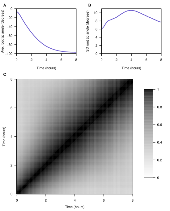
Figure S2: Average (A) and standard deviation (B) of the root tip angle phenotype at each individual time point, and the correlations between time points (C).

We focus on the angle of the root tip, in degrees, over time (averaged across replicates within an RIL), and consider only the first of two replicate data sets examined in Moore et al. (2013). There is genotype data at 234 markers on five chromosomes; the function-valued root tip angle trait was measured at 241 time points (every two minutes for eight hours). The estimated genetic map and the trait values for five randomly selected RIL are displayed in Figure S1. The average and SD of the root tip angle at the individual time points, and the correlations between time points, are displayed in Figure S2.

The data are available at the QTL Archive, http://qtlarchive.org/db/q?pg=projdetails&proj=moore_2013b.

Single-QTL analysis: We first applied interval mapping by Haley-Knott regression (Haley and Knott 1992), considering each time point individually. The results are displayed in Figure 1, with the x-axis representing genomic position and the y-axis representing time, and so each horizontal slice is a genome scan for one time point. We plot a signed LOD score, with the sign representing the estimated direction of the QTL effect: red indicates that lines with the Cvi allele had higher phenotype than the lines with the Ler allele; blue indicates that lines with the Ler allele had higher phenotype than the lines with the Cvi allele.

The most prominent QTL are on chromosomes 1 and 4; in both cases the Cvi allele had higher phenotype than the Ler allele. The chromosome 1 QTL affects later times, and the chromosome 4 QTL affects earlier times. There is an additional QTL of interest on distal chromosome 3, with the Ler allele having higher phenotype at early times.

The SLOD and MLOD statistics combine the results across time points, by taking the average or the maximum LOD, respectively, at each genomic location. The results are in Figure 2A and 2B. Horizontal lines indicate the 5% genome-wide significance thresholds, derived by a permutation test.

We also applied the estimating equations approach of Xiong et al. (2011). This has two variants: a Wald statistic, denoted EE(Wald), and a residual error statistic, denoted EE(Residual). Results are displayed in Figure 2C and 2D, again with horizontal lines indicating the 5% genome-wide significance thresholds.

The 5% significance thresholds for the four methods, derived from permutation tests with 1000 permutation replicates, are shown in Table S1.

All four methods identify QTL on chromosomes 1, 4 and 5. The MLOD and EE(Wald) methods further identify a QTL on chromosome 3, and the EE(Wald) method identifies a further QTL on chromosome 2.

Multiple-QTL analysis: Methods that account for multiple QTL may improve power and better separate evidence for linked QTL. We extended the approach of Broman and Speed (2002) for function-valued traits. Here we focus on additive QTL models, and extend the SLOD and MLOD statistics.

The penalized-SLOD criterion, with the 5% significance threshold as the penalty, indicated a two-QTL model with QTL on chromosomes 1 (at 60 cM) and 4 (at 43 cM). The penalized-MLOD statistic indicated a three-QTL model, with an additional QTL on chromosome 3 (at 76.1 cM). The positions of the QTL on chromosomes 1 and 4 were changed slightly relative to the inferred QTL model by the penalized-SLOD criterion; with the penalized-MLOD criterion, the chromosome 1 QTL was at 62 cM and the chromosome 4 QTL was at 39 cM.

Following an approach developed by Zeng et al. (2000), we derived profile log likelihood curves, to visualize the evidence and localization of each QTL in the context of a multiple-QTL model: The position of each QTL was varied one at a time, and at each location for a given QTL, we derived a LOD score comparing the multiple-QTL model with the QTL under consideration at a particular position and the locations of all other QTL fixed, to the model with the given QTL omitted. This profile is calculated for each time point, individually, and then the SLOD (or MLOD) profiles are obtained by averaging (or maximizing) across time points. The SLOD and MLOD profiles are shown in Figure 3.

To further characterize the effects of the QTL in the context of the inferred multiple-QTL models, we fit the selected multiple-QTL models at each time point, individually. For the models derived by the penalized-SLOD and penalized-MLOD criteria, the estimated baseline function and the estimated QTL effects, as a function of time, are shown in Figure 4. The estimated QTL effects in panels B--D are for the difference between the Cvi allele and the Ler allele.

The effects of the QTL on chromosomes 1 and 4 are approximately the same, whether or not the chromosome 3 QTL is included in the model. The chromosome 1 QTL has greatest effect at later time points, while the chromosome 4 QTL has greatest effect earlier and over a wider interval of time. For both QTL, the Cvi allele increases the root tip angle phenotype. The chromosome 3 QTL, identified only with the penalized-MLOD criterion, has an effect at early time points, and only for a brief interval of time, and for this QTL, the Ler allele increases the root tip angle phenotype.

Simulations

In order to investigate the performance of our proposed approaches and compare them to existing methods, we performed several computer simulation studies. While numerous methods for QTL mapping with function-valued traits have been described, we were unsuccessful, despite considerable effort, to employ the software for Yang et al. (2009), Yap et al. (2009), Min et al. (2011), or Sillanpää et al. (2012). Thus our main focus for comparison was to the estimating equation approach of Xiong et al. (2011). This method has been implemented only for a single-QTL genome scan, and so we compare our approach to that method in the presence of a single QTL. In these single-QTL models, we also considered a simple parametric approach: fit growth curves for each individual (Kahm et al. 2010) and then apply multivariate QTL analysis (Knott and Haley 2000) with the estimated parameters as phenotypes. In the context of multiple-QTL models, we considered only the two variants of our own approach, the penalized-SLOD and penalized-MLOD criteria.

Single-QTL models: To compare our approach to that of Xiong et al. (2011), and to a simple parametric approach, in the context of a single-QTL model, we considered the simulation setting described in Yap et al. (2009), though exploring a range of QTL effects.

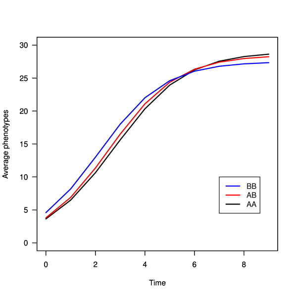
Figure S3: Growth curves for the three QTL genotypes in the single-QTL simulation study.

We simulated an intercross with sample sizes of 100, 200, or 400, and a single chromosome of length 100 cM, with 6 equally spaced markers and with a QTL at 32 cM. The associated phenotypes was sampled from a multivariate normal distribution with the mean curve following a logistic function, $g(t)=\frac{a}{1+be^{-rt}}$. The AA genotype had $a=29,b=7,r=0.7$; the AB genotype had $a=28.5,b=6.5,r=0.73$; and the BB genotype had $a=27.5,b=5,r=0.75$. The shape of growth curve with this parameter shown in Figure S3. Each individual is observed at 10 time points.

The residual error was assumed to be multivariate normal with a covariance structure $c\Sigma$. The constant $c$ controls the overall error variance, and $\Sigma$ was chosen to have one of three different covariance structures: (1) auto-regressive with $\sigma^{2}=3,\rho=0.6$, (2) equi-correlated with $\sigma^{2}=3,\rho=0.5$, or (3) an ‘‘unstructured’’ covariance matrix, as given in Yap et al. (2009) (shown in Table S2).

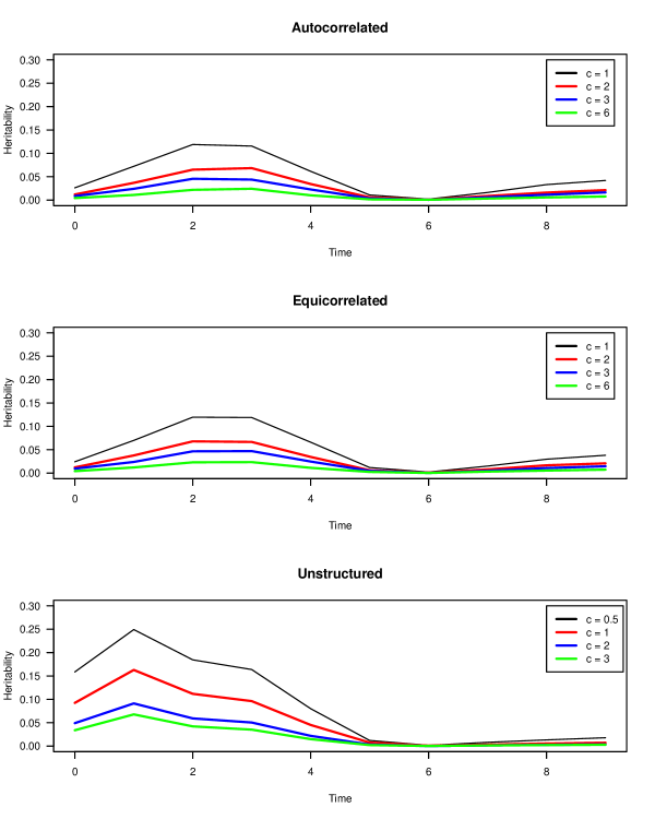
Figure S4: The heritability for each time point in the single-QTL simulation study, for the three assumed variance structures and the chosen values for the $c$ parameter.

The parameter $c$ was given a range of values, which define the percent phenotypic variance explained by the QTL (the heritability). The effect of the QTL varies with time; we took the mean heritability across time as an overall summary. For the auto-regressive and equi-correlated covariance structures, we used $c=1,2,3,6$; for the unstructured covariance matrix, we took $c=0.5,1,2,3$. The heritabilities, as a function of time, for each covariance structure and for each value of the parameter $c$, are shown in Figure S4.

For each of 10,000 simulation replicates, we applied our SLOD and MLOD methods, using Haley-Knott regression (Haley and Knott 1992), and the two versions of the method of Xiong et al. (2011), EE(Wald) and EE(Residual). We further applied a simple parametric approach: We fit the logistic growth model to each individual’s phenotype data using the R package grofit (Kahm et al. 2010), and then used the estimated model parameters as phenotypes, applying the multivariate QTL mapping method of Knott and Haley (2000). For all five approaches, we fit a three-parameter QTL model (that is, allowing for dominance).

The estimated power to detect the QTL as a function of heritability due to the QTL, for $n=100,200,400$ and for the three different covariance structures, is shown in Figure 5. With the autocorrelated variance structure, all methods other than parametric approach gave similar power. With the equicorrelated variance structure, EE(Wald) had higher power than the other four methods, and the parametric approach was second-best. In the unstructured variance setting, EE(Wald) and MLOD method worked better than the other three methods. EE(Residual) didn’t work well in this setting.

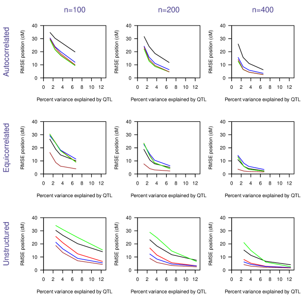
Figure S5: Root Mean Square Error (RMSE) of the estimated QTL position as a function of the percent variance explained by a single QTL. The first column is for $n=100$, the second column is for $n=200$ and the third column is for $n=400$. The three rows correspond to the covariance structure (autocorrelated, equicorrelated, and unstructured). In each panel, SLOD is in red, MLOD is in blue, EE(Wald) is in brown, EE(Residual) is in green, and parametric is in black.

The precision of QTL mapping, measured by the root mean square error in the estimated QTL position, is displayed in Figure S5. Performance, in terms of precision, corresponds quite closely to the performance in terms of power: when power is high, the RMS error of the estimated QTL position is low, and vice versa.

A possible weakness of the SLOD and MLOD approaches, in not making use of the function-valued form of the phenotypes, is that the methods may suffer lower power in the case of noisy phenotypes. To investigate this possibility, we repeated the simulations with $n=200$, adding independent, normally distributed errors (with standard deviation 1 or 2) at each time point.

The estimated power to detect the QTL as a function of heritability due to the QTL, for added noise with SD $=0,1,2$ and the three different covariance structures, is shown in Figure 6. The power of the SLOD, MLOD, the EE(Residual) methods are greatly affected by the introduction of noise. EE(Wald) and the parametric methods are relatively robust to the introduction of noise. Overall, the EE(Wald) method continued to perform best.

For smooth traits with autocorrelated errors, the SLOD and MLOD methods works similarly to EE(Wald) and EE(Residual). However, if we have large measurement error or have different variance structure, the EE(Wald) method is a robust choice. The parametric approach was more affected by the nature of the residual variance structure than by the addition of random noise.

In terms of computation time, in this simulation study, the MLOD and SLOD methods were about 3 times faster than EE(Residual), and they were about 265 times faster than the EE(Wald) method, with five basis functions used in the latter.

Multiple-QTL models: To investigate the performance of the penalized-SLOD and penalized-MLOD criteria in the context of multiple QTL, we simulated data from a three-QTL model modeled after that estimated from the root tip angle data of Moore et al. (2013), considered in the Application section.

We assumed that the mean curve for the root tip angle phenotype followed a cubic polynomial, $y=a+bt+ct^{2}+dt^{3}$, and assumed that the effect of each QTL also followed such a cubic polynomial. Fitting this parametric model with the three QTL derived by the penalized-MLOD criterion, we obtained the following estimates. The parameters of the baseline were $(a,b,c,d)=(-0.238,-265.248,229.405,-59.771)$. The QTL effect for the QTL chromosome 1 at 61 cM had parameters $(0.209,8.729,1.602,-9.054)$. A second QTL, on chromosome 3 at 76 cM, had parameters $(-1.887,3.414,-4.220,2.265)$. The third QTL, on chromosome 4 at 40 cM, had parameters $(2.003,11.907,-28.647,15.311)$. The baseline function and the QTL effect curves are shown in Figure S5.

The four parameters for a given individual were drawn from a multivariate normal distribution with mean defined by the QTL genotypes and variance matrix estimated from the root tip angle data as:

$$\Sigma=\begin{pmatrix}58.99&-177.77&185.11&-45.44\\ -177.77&3848.70&-7274.83&3595.37\\ 185.11&-7274.83&16897.56&-9702.32\\ -45.44&3595.37&-9702.32&6096.71\\ \end{pmatrix}$$

In addition, normally distributed measurement error (with mean 0 and variance 1) was added to the phenotype at each time point for each individual. Phenotypes are taken at 241 equally spaced time points in the interval of 0 to 1. We considered two sample sizes: $n=162$ (as in the Moore et al. (2013) data) and twice that, $n=324$.

We performed 2000 simulation replicates. For each replicate, we applied a stepwise model selection approach with each of the penalized-SLOD and penalized-MLOD criteria. The simulation results are shown in Table 1.

The penalized-SLOD criterion had higher power to detect the first and third QTL, while the penalized-MLOD criterion had higher power to detect the second QTL. With the larger sample size, the power to detect QTL increased, and the standard error of the estimated QTL position decreased.

The estimated false positive rates at $n=162$ were 3.3 and 0.9% for the penalized-SLOD and penalized-MLOD criteria, respectively. At the larger sample size, $n=324$, the corresponding false positive rates were 4.1 and 0.8%.

Discussion

Automated phenotype measurement is an accelerating trend across biological scales, from microorganisms to crop plants. This push for increasing automation makes it feasible to increase the dimensionality of phenotype data sets, for example by adding time. The trend toward higher-dimensional phenotype data sets from genetically structured populations has created a need for new statistical genetic methods, and computational speed can be an important factor in the application of such methods.

Methods for the genetic analysis of function-valued phenotypes have mostly focused on single-QTL models (Ma et al. 2002; Yang et al. 2009; Yap et al. 2009; Xiong et al. 2011). Bayesian multiple-QTL methods, using Markov chain Monte Carlo, have also been proposed (Min et al. 2011; Sillanpää et al. 2012), but they can be computationally intensive and not easily implemented. We propose two simple LOD-type statistics that integrate the information across time points and extend them, using the approach of Broman and Speed (2002), for multiple-QTL model selection.

The basis of our approach is the analysis of each time point individually. This works well when the function-valued trait is smooth, as in the data from Moore et al. (2013), and has the benefit of providing results that are easily interpreted, such as the QTL effects displayed in Figure 4. With unequally-spaced time points or appreciable missing data, the approach may require some modification, such as first performing some interpolation or smoothing. The performance of our approaches deteriorated with added noise, but again this may be at least partly alleviated by pre-smoothing. An important advantage of our approach is the ability to incorporate information from multiple QTL in the analysis of function-valued phenotypes, which should improve power and lead to better separation of linked QTL.

A weakness of our approach is that it largely ignores the correlations across time. Ma et al. (2002) and Yang et al. (2009) paid careful attention to this aspect, using an autoregressive model for the residual variance matrix. Our current neglect of this aspect may result in loss of efficiency, particularly in the estimates of the QTL effects. However by ignoring this assumption we gain much speed, and our simulation studies indicate that the approach exhibits reasonable power to detect QTL in many situations. The EE(Wald) method of Xiong et al. (2011) showed the best performance among all methods considered, though at the expense of considerably greater computation time.

Manichaikul et al. (2009) extended the work of Broman and Speed (2002) by considering pairwise interactions among QTL. Our approach may be similarly extended to consider interactions.

An alternative approach to the QTL analysis of function-valued traits is to first fit a parametric model to each individual’s curve and then treat the estimated parameters from such a model as phenotypes. (The method exhibited less-than-ideal performance in our simulation study, likely due to poor model fit with the simulated error structures.) Multiple-QTL mapping methods could readily be applied to each such parameter, individually. The advantage of our approach, to consider each time point individually, is in the simpler interpretation of the results.

Software implementing our methods have been implemented as a package for R (R Core Team 2013), funqtl (https://github.com/ikwak2/funqtl).

Acknowledgments

The authors thank Śaunak Sen and two anonymous reviewers for comments to improve the manuscript. This work was supported in part by grant IOS-1031416 from the National Science Foundation Plant Genome Research Program to E.P.S. and by National Institutes of Health grant R01GM074244 to K.W.B.

Table 1: Simulation results for the SLOD and MLOD criteria, for a three-QTL model modeled after the Moore et al. (2013) data.

		Mean (SE) estimated location			Power
	True location	SLOD	MLOD		SLOD	MLOD
$n$=162	61	60.9 (6.1)	61.1 (4.9)		89	54
	76	65.0 (18.3)	71.4 (11.5)		12	15
	40	40.0 (4.9)	40.4 (3.4)		82	77
$n$=324	61	61.3 (2.6)	61.3 (3.8)		100	59
	76	72.0 (9.7)	74.5 (4.8)		31	43
	40	40.0 (2.1)	40.1 (2.0)		100	91

Note: Locations are in cM.

Figure Legends

• Figure 1. Signed LOD scores from single-QTL genome scans, with each time point considered individually.

• Figure 2. The SLOD, MLOD, EE(Wald) and EE(Residual) curves for the root tip angle data. A red horizontal line indicates the calculated 5% permutation-based threshold.

• Figure 3. SLOD and MLOD profiles for a multiple-QTL model for the root tip angle data set.

• Figure 4. The regression coefficients estimated for the root tip angle data set. The red curves are for the two-QTL model (from the penalized-SLOD criterion) and the blue dashed curves are for the three-QTL model (from the penalized-MLOD criterion). Positive values for the QTL effects indicate that the Cvi allele increases the tip angle phenotype.

• Figure 5. Power as a function of the percent phenotypic variance explained by a single QTL. The first column is for $n=100$, the second column is for $n=200$ and the third column is for $n=400$. The three rows correspond to the covariance structure (autocorrelated, equicorrelated, and unstructured). In each panel, SLOD is in red, MLOD is in blue, EE(Wald) is in brown, EE(Residual) is in green, and parametric is in black.

• Figure 6.Power as a function of the percent phenotypic variance explained by a single QTL, with additional noise added to the phenotypes. The first column has no additional noise; the second and third columns have independent normally distributed noise added at each time point, with standard deviation 1 and 2, respectively. The three rows correspond to the covariance structure (autocorrelated, equicorrelated, and unstructured). In each panel, SLOD is in red, MLOD is in blue, EE(Wald) is in brown, EE(Residual) is in green, and parametric is in black. The percent variance explained by the QTL on the x-axis refers, in each case, to the variance explained in the case of no added noise.

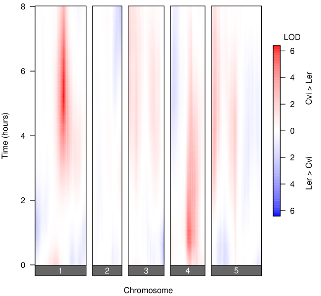
Figure 1: Signed LOD scores from single-QTL genome scans, with each time point considered individually.

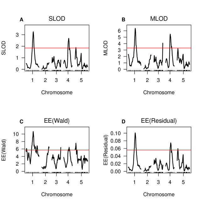
Figure 2: The SLOD, MLOD, EE(Wald) and EE(Residual) curves for the root tip angle data. A red horizontal line indicates the calculated 5% permutation-based threshold.

Figure 3: SLOD and MLOD profiles for a multiple-QTL model with the root tip angle data set.

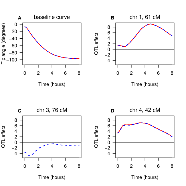
Figure 4: The regression coefficients estimated for the root tip angle data set. The red curves are for the two-QTL model (from the penalized-SLOD criterion) and the blue dashed curves are for the three-QTL model (from the penalized-MLOD criterion). Positive values for the QTL effects indicate that the Cvi allele increases the tip angle phenotype.

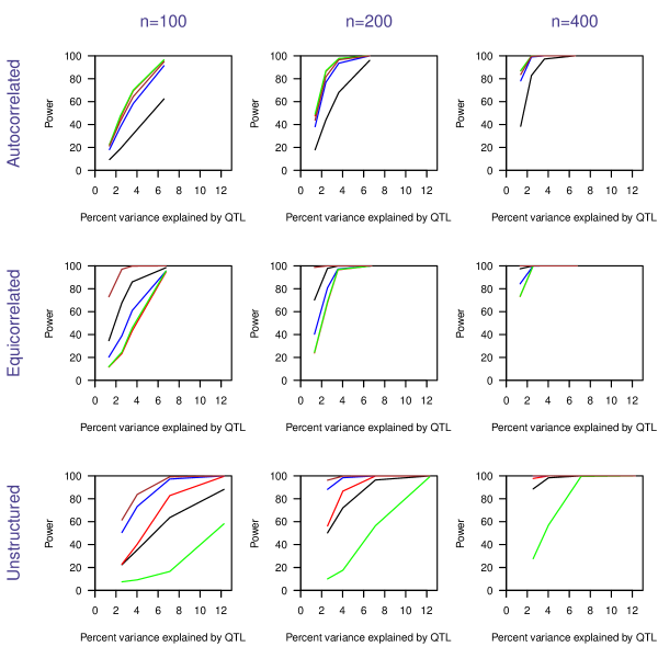
Figure 5: Power as a function of the percent phenotypic variance explained by a single QTL. The first column is for $n=100$, the second column is for $n=200$ and the third column is for $n=400$. The three rows correspond to the covariance structure (autocorrelated, equicorrelated, and unstructured). In each panel, SLOD is in red, MLOD is in blue, EE(Wald) is in brown, EE(Residual) is in green, and parametric is in black.

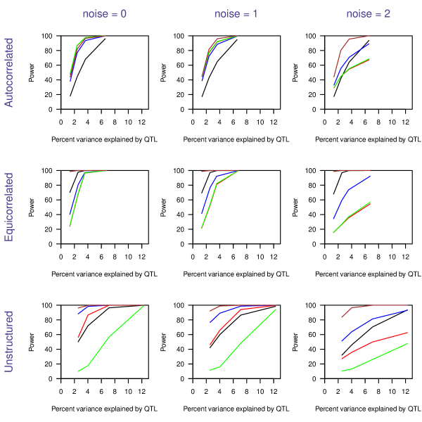
Figure 6: Power as a function of the percent phenotypic variance explained by a single QTL, with additional noise added to the phenotypes. The first column has no additional noise; the second and third columns have independent normally distributed noise added at each time point, with standard deviation 1 and 2, respectively. The three rows correspond to the covariance structure (autocorrelated, equicorrelated, and unstructured). In each panel, SLOD is in red, MLOD is in blue, EE(Wald) is in brown, EE(Residual) is in green, and parametric is in black. The percent variance explained by the QTL on the x-axis refers, in each case, to the variance explained in the case of no added noise.

15 May 2014

Figure S1: Genetic map of typed genetic markers (A) and function-valued phenotypes for five randomly selected Arabidopsis RIL (B), for data from Edgar Spalding and colleagues.

Figure S6: Root Mean Square Error (RMSE) of the estimated QTL position as a function of the percent variance explained by a single QTL, with additional noise added to the phenotypes. The first column has no additional noise; the second and third columns have independent normally distributed noise added at each time point, with standard deviation 1 and 2, respectively. The three rows correspond to the covariance structure (autocorrelated, equicorrelated, and unstructured). In each panel, SLOD is in red, MLOD is in blue, EE(Wald) is in brown, EE(Residual) is in green, and parametric is in black. The percent variance explained by the QTL on the x-axis refers, in each case, to the variance explained in the case of no added noise.

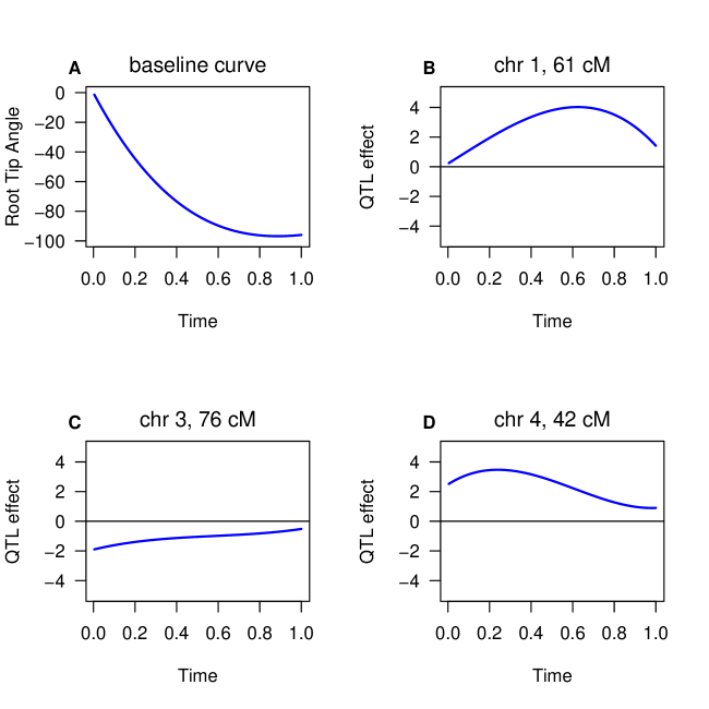
Figure S7: The underlying true baseline function (A) and QTL effect curves (B, C and D) for the multiple-QTL simulations.

Table S2: 5% significance thresholds for the data from Moore et al. 2013, based on a permutation test with 1000 replicates.

Method	Threshold
SLOD		1.	85
MLOD		3.	32
EE(Wald)		5.	72
EE(Residual)		0.	0559

Table S3: The unstructured covariance matrix used in the single-QTL simulations.

$$\Sigma=\begin{pmatrix}0.72&0.39&0.45&0.48&0.50&0.53&0.60&0.64&0.68&0.68\\ 0.39&1.06&1.61&1.60&1.50&1.48&1.55&1.47&1.35&1.29\\ 0.45&1.61&3.29&3.29&3.17&3.09&3.19&3.04&2.78&2.53\\ 0.48&1.60&3.29&3.98&4.07&4.01&4.17&4.18&4.00&3.69\\ 0.50&1.50&3.17&4.07&4.70&4.68&4.66&4.78&4.70&4.36\\ 0.53&1.48&3.09&4.07&4.68&5.56&6.23&6.87&7.11&6.92\\ 0.60&1.55&3.19&4.17&4.66&6.23&8.59&10.16&10.80&10.70\\ 0.64&1.47&3.04&4.18&4.78&6.87&10.16&12.74&13.80&13.80\\ 0.68&1.35&2.78&4.00&4.70&7.11&10.80&13.80&15.33&15.35\\ 0.68&1.29&2.53&3.69&4.36&6.92&10.70&13.80&15.35&15.77\\ \end{pmatrix}$$

Literature Cited

- Broman and Speed (2002) Broman, K. W., and T. P. Speed, 2002 A model selection approach for the identification of quantitative trait loci in experimental crosses. J. R. Statist. Soc. B 64: 641--656.
- Churchill and Doerge (1994) Churchill, G. A., and R. W. Doerge, 1994 Empirical threshold values for quantitative trait mapping. Genetics 138: 963--971.
- Haley and Knott (1992) Haley, C. S., and S. A. Knott, 1992 A simple regression method for mapping quantitative trait loci in line crosses using flanking markers. Heredity 69: 315--324.
- Kahm et al. (2010) Kahm, M., G. Hasenbrink, H. Lichtenberg-Fraté, J. Ludwig, and M. Kschischo, 2010 grofit: Fitting biological growth curves with R. J. Statist. Softw. 33: 1--21.
- Kendziorski et al. (2002) Kendziorski, C. M., A. W. Cowley, A. S. Greene, H. C. Salgado, H. J. Jacob et al., 2002 Mapping baroreceptor function to genome: a mathematical modeling approach. Genetics 160: 1687--1695.
- Knott and Haley (2000) Knott, S. A., and C. S. Haley, 2000 Multitrait least squares for quantitative trait loci detection. Genetics 156: 899--911.