Group Momentum Space and Hopf Algebra Symmetries in Gravity
Group Momentum Space and Hopf Algebra
Symmetries of Point Particles Coupled
to Gravity⋆⋆\star⋆⋆\starThis paper is a contribution to the Special Issue on Deformations of Space-Time
and its Symmetries.
The full collection is available at http://www.emis.de/journals/SIGMA/space-time.html
Michele ARZANO †, Danilo LATINI ‡ and Matteo LOTITO §
M. Arzano, D. Latini and M. Lotito
† Dipartimento di Fisica and INFN, “Sapienza” University of Rome, P.le A. Moro 2,
00185 Roma, Italy
\EmailDmichele.arzano@roma1.infn.it
‡ Dipartimento di Fisica and INFN, Università di Roma Tre, Via Vasca Navale 84,
I-00146 Roma, Italy
\EmailDlatini@fis.uniroma3.it
§ Department of Physics, University of Cincinnati, Cincinnati, Ohio 45221-0011, USA \EmailDlotitomo@mail.uc.edu
Received March 13, 2014, in final form July 15, 2014; Published online July 24, 2014
We present an in-depth investigation of the momentum space describing point particles coupled to Einstein gravity in three space-time dimensions. We introduce different sets of coordinates on the group manifold and discuss their properties under Lorentz transformations. In particular we show how a certain set of coordinates exhibits an upper bound on the energy under deformed Lorentz boosts which saturate at the Planck energy. We discuss how this deformed symmetry framework is generally described by a quantum deformation of the Poincaré group: the quantum double of . We then illustrate how the space of functions on the group manifold momentum space has a dual representation on a non-commutative space of coordinates via a (quantum) group Fourier transform. In this context we explore the connection between Weyl maps and different notions of (quantum) group Fourier transform appeared in the literature in the past years and establish relations between them.
gravity; Lie group momentum space; deformed symmetries; Hopf algebra
81R50; 83A05; 83C99
1 Introduction
General relativity in three space-time dimensions offers an unparalleled insight on how quantum group deformed relativistic symmetries replace ordinary structures linked to the Poincaré group.
The simple picture is that relativistic point particles are coupled to the theory as conical defects owing to the topological nature of Einstein gravity in three dimensions [15, 31]. For vanishing cosmological constant the resulting space-time is flat everywhere except at the location of the particle, the conical singularity. The parametrization of a moving defect, like e.g. the conical particle, requires their momentum to be described by an element of the isometry group of the ambient space. In our specific case it turns out that momenta are no longer vectors in three dimensional Minkowski space but elements of the double cover of the Lorentz group in three dimensions, [23, 29]. Lorentz transformations are easily implemented for this curved momentum space in terms of the action of on itself.
At the group theoretic level such transition from vector-like to group-like momenta is captured by the transition from the (group algebra of) the Poincaré group to the quantum double of , a non-trivial Hopf algebra in which the three-dimensional Newton’s constant appears as a deformation parameter [11, 12]. Functions on provide now the space on which representations of the double of are defined [9, 21]. A notion of Fourier transform can be introduced which maps these functions on a group onto functions of non-commutative space in which coordinates obey non-trivial commutation relations given by the brackets of the Lie algebra of [17, 28]. Alternatively one can map these functions onto ordinary three-dimensional Minkowski space equipped with a non-commutative star-product determined by the non-abelian group structure of [16]. Thus the study of relativistic point particles coupled to three-dimensional gravity leads us to consider all the important aspects of deformation of relativistic symmetries and non-commutativity within a clear geometric picture.
Our aim in this work will be to review the main features discussed above and point out some new results which will help link the structures emerging in this three-dimensional context to other models of deformed symmetries and non-commutativity in four space-time dimensions.
We start in the next section by reviewing how momenta of conical defects in three dimensions are parametrized by group elements. In particular we show how the usual notion of mass-shell describing the momentum of physical particles is replaced by the condition that group valued momenta belong to the conjugacy class of a rotation by a deficit angle characterizing the conical defect. In Section 3 we describe coordinate systems on starting with two choices which are popular in the literature and introducing a new parametrization based on Euler angles. For each parametrization we write down the explicit form of the conjugacy class condition which represents the realization of a deformed mass-shell in each choice of coordinates and show that for the new parametrization introduced on-shell momenta exhibit a maximum energy. Furthermore we discuss the action of Lorentz transformations on the momentum space case by case. In particular we show that the Euler angle coordinates transform non-linearly under the action of a boost and that the energy saturates at the maximum value when the boost parameter is let to infinity. Thus we find a set of momentum coordinates which provide an explicit realization of doubly special relativity for a particle coupled to three-dimensional gravity [5, 7]. In Section 4 we review what is the structure of the underlying quantum group symmetry associated with the momentum space given by the quantum double of and we show how such Hopf algebra can be obtained as a deformation of the group algebra of the Poincaré group. Next we discuss non-commutative plane waves with momenta and the associated notions of (quantum) group Fourier transform (a thorough investigation on this and a detailed description of the symmetries arising in this context can be found in the recent work [30]). This gives us the opportunity to clarify the connection between different notions of Fourier transform appearing in the literature and to discuss their relation with Weyl maps which have been extensively used in the literature on non-commutative space-times in dimensions [2, 3, 24]. Finally we provide a master equation for the group Fourier transform which for each choice of Weyl map, corresponding to a given group parametrization, reproduces the different group Fourier transforms appeared in the literature. Section 5 is devoted to brief concluding remarks.
2 The momentum space of particles coupled
to -dimensional gravity
2.1 Particles as conical defects in gravity
General relativity in three space-time dimensions has the well known property of not possessing local degrees of freedom. All solutions of Einstein’s equations with vanishing cosmological constant are locally flat and the only non-trivial degrees of freedom have to be of topological nature. This must be taken into account when coupling particles to the theory. Indeed, as already shown by Staruszkiewicz in his seminal work [31], later thoroughly extended by Deser, Jackiw and ’t Hooft [15], point-like degrees of freedom carrying mass and spin can be added introducing “punctures” on the space-time (flat) manifold. In the simplest case of a spinless particle, which will be of interest for the present work, one can picture such a puncture as creating a conical singularity resulting in a space-time which is flat everywhere except at the location of the particle (see Fig. 1).
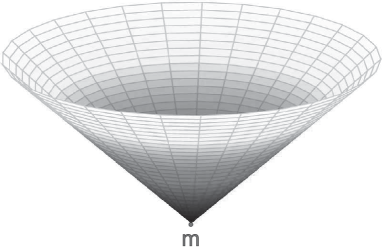
This conical space can be characterized by a deficit angle where is the mass of the particle and is Newton’s constant in three dimensions.
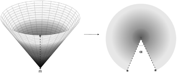
The deficit angle is simply the angle formed by the missing wedge obtained when “opening up” the conical space on a flat Minkowski space (see Fig. 2). The metric of such conical space-time is given by
with the azimuthal angle having period . Alternatively we can write the metric keeping the angular -coordinate with a period as:
The deficit angle can be measured by calculating the holonomy of the connection associated to the metric along a loop encircling the particle. This describes the parallel transport of a vector around the singularity [23], which results in a rotation by an angle . Roughly speaking we have that the mass, i.e. the three-momentum at rest of the point particle/defect, is characterized by a rotation proportional to the mass of the particle multiplied by Newton’s constant.
To characterize the physical momentum of a moving defect let us briefly recall how physical momenta of a relativistic point particle are described in ordinary Minkowski space. In three space-time dimensions Minkowski space is isomorphic, as a vector space, to , the algebra of the Lie group .111For our readers convenience we recall the basic properties of the group in Appendix A. If is a basis of traceless matrices, given an element and a vector we can write [23]
Momenta are thus given by the following algebra element
whose determinant is . We can describe physical momenta by boosting the momentum at rest of a particle. The latter will be given in matrix representation by and the boost is achieved via the adjoint action of on so that a physical momentum will be given by
| (2.1) |
Such action preserves the determinant and the physical momenta, obtained by boosting the three momentum at rest, will be characterized by the mass-shell condition
We thus have that in three-dimensional Minkowski space the extended momentum space of a relativistic point particle can be identified with and the physical momenta belong to orbits of on which determine the mass-shell.
We can now have an intuitive characterization of the momentum space of a moving conical defect in three dimensions (for more formal discussions we refer the reader to [9, 23]). As discussed above the momentum at rest of a conical defect can be parametrized by a rotation , i.e. a group element rather than the vector . The action of a Lorentz boost on the momentum at rest will be described just by an action of on itself
| (2.2) |
and thus physical momenta of a defect of mass will be given by elements of belonging to the conjugacy class of a rotation by an angle . Therefore, when gravity is switched on, the extended momentum space of a point particle is given by the group manifold (to be contrasted with the vector space in the ordinary Minkowski case) while its physical momentum space is given by the action by conjugation of on the momentum at rest (to be contrasted with the adjoint action in the ordinary case) [9, 23]. In Section 4.2 we will discuss how the transition from vector valued momenta to group valued momenta viz. from equation (2.1) to (2.2) can be understood from a mathematical point of view in terms of a lift morphism between functions on Minkowski space to functions on . Physically speaking the transition from (2.1) to (2.2) simply reflects the fact that the phase space of a point particle coupled to gravity is the cotangent bundle of with the latter describing the momentum degrees of freedom222Very similar structures arise in loop quantum gravity and group field theory where the configuration space is given by a Lie group, see e.g. [13, 14, 26]. of the particle [23]. In the next section we give a detailed account of the group momentum space of the particle and of the classification of the conjugacy classes describing “on-shell” momenta.
2.2 Conjugacy classes as deformed mass-shell
In order to introduce the conjugacy classes of the group we start by recalling the expansion of the generic group element in terms of the unit and the matrices:
| (2.3) |
which can be written in the following matrix form:
| (2.4) |
The unit determinant condition on this matrix gives and thus the parameter can be expressed in terms of the other free parameters and can be either positive or negative. If we were considering instead of the proper orthocronous Lorentz group positive and negative values of would be identified. This reflects the fact that is a double cover of . Now the action by conjugation of on itself leaves the trace invariant, therefore the number is an invariant under action by conjugation. In particular, the group is composed by five different subclasses, called conjugacy classes, which are invariant under conjugation [10]. These subclasses can be described by the eigenvalues of the matrix (2.4). The secular equation for the generic element of reads
whose solutions are given by
We can now classify group elements according to their trace, in fact we see that the above equation has different behaviours according to the value of the discriminant , in particular the sign of this term will determine the different sets of solutions, i.e. group elements:
- •
- •
- •
To make contact with the ordinary classification of particles according to the sign of their mass squared, we have here that a group element obtained by conjugating the momentum at rest of a gravitating particle
belongs to the class of elliptic transformations, which represent massive particles. Analogously, hyperbolic elements will represent tachyons and the parabolic elements photons as we can deduce by taking the limit and checking that for the former we have a negative mass squared, while for the latter the mass is vanishing.
The deformed mass-shell condition assigning a group element to the conjugacy class describing massive particles can be obtained by putting a constraint on its trace which, in light of what we said above, will be given by
| (2.5) |
with where we defined a new deformation parameter with dimensions of mass for later convenience. This range of masses implies a choice of positive sign of the variable discussed above. This choice of sign, widely adopted in the literature, is mathematically equivalent to considering the quotient , where is the cyclic group.
In what follows, we will give concrete examples of group parametrizations and their (deformed) mass-shell, before moving on to the description of how relativistic symmetries are implemented for such particles.
3 Coordinates and symmetries on the momentum space
In this section we recall some known parametrizations of group elements/momenta and introduce others which will help us get insight on the kinematical properties associated to each set of coordinates. Furthermore, we will implement Lorentz transformations in the picture discussing how these are realized for each choice of parameterization adopted.
3.1 Cartesian coordinates
Cartesian coordinates on the group manifold are the most used in the literature. They are based on the parametrization (2.3) which we introduced in Section 2.2
We define
where we introduced the notation , , so that the group parameters are dimensionless and the coordinates have the dimensions of energy. The deformed mass-shell constraint (2.5) in Cartesian coordinates reads
which after easy manipulations gives
| (3.1) |
In the limit the dispersion relation (3.1) reproduces the usual mass-shell relation valid for an ordinary (flat) momentum space of a massive particle, i.e. . The deformation given by the gravity effects, using this parametrization, appears as a renormalization of the mass which is no longer but .
3.1.1 Boosts for Cartesian coordinates
We show now how momenta described by cartesian coordinates transform under Lorentz boosts. Without loss of generality we consider a Lorentz boost in -direction. This is represented by the group element where is the boost rapidity. The action of on itself is realized by conjugation
which in components will read
Writing down the product on the right hand side above, using the multiplication properties of the matrices and putting together the terms proportional to the same matrix we obtain the expressions for the boosted parameters in terms of the old parameters
We thus obtain the ordinary action of a Lorentz boost in the direction.
3.2 Exponential coordinates
This set of coordinates is widely used in the works on Euclidean models (see e.g. [19]) in which is considered instead of . The parametrization is defined as follows (see also [27])
It is trivial to check that for this parametrization the determinant constraint is satisfied
and a generic group element can be written in terms of -coordinates as
where the last equality shows that this parametrization is equivalent to considering the exponential of the generators, from this the name “exponential coordinates”. The conjugacy class constraint this time leads to the mass-shell condition
which is just an ordinary mass-shell relation where, however, the values of the mass are limited by due to the limits on the deficit angle.
3.2.1 Boosts for exponential coordinates
As in the previous case we consider the action by conjugation of the Lorentz boost in a -direction
In analogy with the previous case we can find an explicit expression for the boosted parameters using the matrix expansion of the exponentials
and thus also the exponential coordinates transform as ordinary momenta in Minkowski space under a boost.
3.3 Time-symmetric parametrization: Euler coordinates
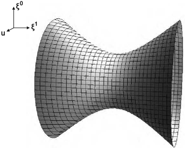
In this section we develop a set of coordinates on based on a choice of energy and linear momentum introduced in earlier works on the coupling of point particles to gravity [23, 32, 33]. The idea is to describe the momenta of a gravitating particle using a parametrization in terms of angles (closely related to the Euler angles parametrizing )
where and (see Fig. 3).
Now, using this set of coordinates, we can rewrite the expansion of the group element in terms of the matrices as [23]:
This choice of coordinates shows clearly that the Lorentz transformation represented by is decomposed in a spatial rotation of angle in the plane , a boost in direction with the parameter and another rotation in the same plane of the previous but by angle .
In order to interpret our coordinates as momenta we rewrite the expansion of the group element using and as dimensionful parameters and , obtaining
Now, as in the previous cases, if we impose the condition which projects the group element into the conjugacy class of rotations, i.e. , we obtain
| (3.2) |
which is the deformed mass-shell relation in our new coordinates. If we take the limit
which, simplifying the leading terms and identifying the terms proportional to , gives
Such equation reproduces an ordinary relativistic mass-shell relation if one identifies and respectively with the energy and the norm of the spatial momentum. This leads us to define the following momenta for the gravitating particles
In terms of the new -coordinates we have
Using this parametrization, the generic group element can be written as
| (3.3) |
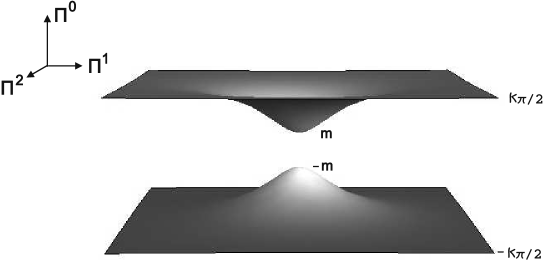
as shown in detail in Appendix B. The mass-shell relation (3.2) can be rewritten in terms of the momenta as
which solved for the energy gives
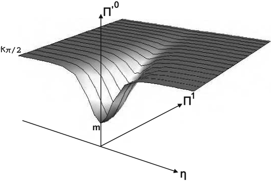
showing that the energy is limited by the range values (see Fig. 4). This was somewhat an expected result, since the energy in this set of coordinates is proportional to the deficit angle but we will have more to say about this feature when considering Lorentz transformations in the next sections.
3.3.1 Boosts on Euler coordinates
Again, we can compute the expression using the same steps of the previous cases.
This leads us to write the following system
whose solution is given by
| (3.4) | |||
We thus have that Euler coordinates on the provide a non-linear realization of Lorentz boosts (see Fig. 5). Obviously in the limit the transformations (3.4) become just ordinary Lorentz boosts. Consider now a particle initially at rest (namely , ), the system of equations (3.4) simplifies to
We see that in the limit when the boost parameter goes to infinity, , the energy does not grow arbitrarily but saturates at the value . We thus have that the non-linear realization of Lorentz boosts given in Euler coordinates is just an example of deformed or doubly special relativity [5, 6] in which we have a maximum energy built in the deformed structure of Lorentz transformations.
4 The quantum double of
In this section we show how the transition from a Minkowski to momentum space translates for the structure of relativistic symmetries in a deformation of the Poincaré group to the quantum double of , a quantum group denoted as . We start by recalling the definition and Hopf algebra properties of . For a gentle introduction to the necessary notions of Hopf algebras we refer the reader to [18] while a rigorous introduction to can be found in [21].
The quantum double is defined, as a vector space, by the tensor product [20]
where is the space of complex functions on and the group algebra of which, roughly speaking, can be thought of as a vector space comprised by the elements of the group itself. Let us denote an element of the double as , the Hopf algebra structure is given by
| product: | |||
| co-product: | |||
| unit: | |||
| co-unit: | |||
| antipode: | |||
| complex conjugate: |
where and . The explicit expression for the co-product on is given by
telling us that for such space the co-product is simply a way of extending the notion of function on the group to a tensor product of the latter in a way compatible with the composition of the group.
4.1 as a deformation of
Here we show how the quantum double of can be interpreted as a deformation of the group algebra of the three dimensional Poincaré group, or inhomogenous Lorentz group . The group algebra is defined as a vector space by the tensor product
where is the group of translations which we denote as with . The group algebra is the set of elements , with a function (or distribution) with compact support. can be identified with a subalgebra of functions on . This means that for any element of the group algebra we can associate a function whose Fourier transform has compact support. This amounts to identify
In conclusion, the group algebra can be identified with the tensor product
At this point it is evident that the difference with the quantum double is that we have instead of . Thus the connection between and is a “lift” or “deformation map” from to . This will turn out to be an algebra but not a co-algebra morphism [20] since the structure of the co-product for will be different than the one for .
To obtain this map we write down the Hopf algebra structure of
| product: | |||
| co-product: | |||
| unit: | |||
| co-unit: | |||
| antipode: | |||
| complex conugate: |
where the inverse map is defined as in the quantum double where is a vector representation of . The explicit expression for the co-product of is given by
| (4.1) |
which differs from the co-product for since the composition law of the arguments of is abelian while in the co-product for is not. Notice however that the Hopf algebra structure of is very similar to the one of the quantum double of . In particular instead of the map we now have , thus to pass from one Hopf algebra to the other we need a connection between the two maps. In other words we are looking for an algebra morphism such that
where is lifted to . Looking at the two Hopf algebra structures it is clear that the morphism should satisfy the relation
which written explicitly reads
Clearly the morphism depends on the choice of group parametrization [20] indeed each sets of coordinates on can be used to map into . Below we will see how group parametrization are associated to different examples of non-commutative plane waves (as it has been shown for [17, 19, 25]) and we will link them to the notion of Weyl map used in the literature on non-commutative space-times.
4.2 Non-commutative plane waves and Weyl maps
In order to establish a link between plane waves and Weyl maps we start by reviewing the different notions of non-commutative plane waves that are found in the literature on non-commutative spaces in dimensions in connection with momentum space.
The -product, that is customarily introduced on in the literature on discrete Euclidean quantum gravity models [16, 17], in the Lorentzian case is defined by
| (4.2) |
where are coordinates of , . The group element appearing in the plane wave is taken in the Cartesian parametrization . These plane waves can be obtained through a map given by
where is the set of functions on equipped with the -product (4.2). In this way we have an ordinary plane wave equipped with a non-commutative star-product determined by the non-abelian composition rule of the group , which at leading order in the deformation parameter reads
where .
Another set of plane waves [22] labelled by the group element is given in terms of the map
| (4.3) |
where is the non commutative version of , i.e. coordinates on equipped with the non trivial Lie bracket
| (4.4) |
Thus can be seen as the universal enveloping algebra [17]. The in (4.3) are the exponential coordinates introduced before
Notice that the map clearly depends on the group parametrization. Indeed using Cartesian coordinates we have
The same could be repeated for other sets of coordinates. The different plane waves will be linked by a map such that
This map is an isomorphism between algebras, in particular considering the product of two non-commuting functions we have
Notice that the map such that
can be interpreted as a Weyl map [3]. Indeed the -product can be written in terms of as
| (4.5) |
just as in the case of Weyl maps for Lie algebra non-commutative space-times in dimensions as discussed for example in [2]. Notice how the notion of -product defined on commuting function depends on the choice of Weyl map .
4.3 (Quantum) group Fourier transform
The non-commutative plane wave is associated to a notion of quantum group Fourier transform which maps functions on a -dimensional Lie group to functions in [17]:
In the case of associated to the non-commutative plane wave we have
where the Haar measure on the group is expressed in terms of “exponential” coordinates (see Appendix D for a review of the Haar measure in the various parametrizations). This Fourier transform is related to the group Fourier transform discussed in [4, 16, 26] via the map introduced in the previous section. Indeed the following diagram holds
The composition of maps is the group Fourier transform
Notice that the quantization maps discussed in [19] in our picture coincides with the Weyl map in (4.5). Moreover if we change coordinates on the group and pass from the plane wave in exponential coordinates to cartesian coordinates
the quantum group Fourier transform by construction will read
Below we show how to describe these Fourier transforms in a unified framework.
4.4 The master Fourier transform
In this section we exhibit an alternative route to construct non-commutative plane waves and the quantum group Fourier transform. This will lead us to an implicit definition of both which for each group parametrization reproduces the corresponding Fourier transforms found in the literature. We start by considering the group elements written in the three different sets of coordinates introduced above
If we take the generators of the algebra as , we immediately recover the non-commutative plane waves introduced above, in the cartesian and exponential parametrization, and we also obtain a new plane wave for the parametrization
where the coordinates obey the non-trivial Lie bracket (4.4). Notice also that the plane wave in the parametrization is known in the literature on non-commutative spaces as the “time symmetrized” plane wave and has an associated Weyl map [1, 2]. The quantum group Fourier transform for the three sets of coordinates reads
Now we can introduce a formal expression which defines the quantum group Fourier transform in terms of a generic group element .
We define a master plane wave (for 333For the case of we simply substitute hyperbolic functions with trigonometric functions and Pauli matrices instead of matrices.) given by
where . It is easy to show that this definition of plane waves reproduces all the cases above. We can thus write down an implicit definition of Fourier transform, the master quantum group Fourier transform
| (4.6) |
where
Equation (4.6) provides a formal definition of (quantum) group Fourier transform which reproduces the known Fourier transforms appeared in the literature when a quantization/Weyl map is specified444The implicit Fourier transform (4.6) is analogous to the general form of “non-commutative” Fourier transform discussed in Section IV of [19].. We conclude by stressing that the choice of quantization (Weyl) map determines uniquely the form of the plane waves entering the (non-commutative) Fourier transform and is equivalent to a choice of coordinates on the Lie group momentum space [19].
5 Conclusions
In this work we offered a quick, but we hope comprehensive, journey through the notions of deformed symmetry and non-commutativity which are encountered in the study of a relativistic point particle coupled to three-dimensional gravity. In doing so we reviewed and clarified various notions that appear scattered in the literature but also provided some valuable new insights on these models.
On one side we showed for the first time, introducing the new set of Euler coordinates, how the framework of doubly or deformed special relativity is realized in the context of momentum space. In particular we showed that the model considered introduces a notion of maximal energy which is compatible with a deformed action of boosts on momenta living on a group manifold. From a more abstract point of view we connected several important notions which have appeared in the past in the literature on non-commutative spaces with those recently studied within the community working on group field theory [13, 14]. Specifically we clarified the status of the different notions of (quantum) group Fourier transforms appearing in the literature and we were able to formulate an implicit master Fourier transform which, for each choice of star-product or Weyl map, reproduces the various group Fourier transforms proposed in the literature. Particularly significant is the explicit connection we established between different notions of group Fourier transforms, Weyl maps and choices of coordinates on the momentum group manifold. Such connection provides further evidence that models resulting from different quantizations/Weyl maps correspond to different physical scenarios [8]. Moreover our findings bridge an important gap between the two fields and we believe this work will provide a useful reference for those seeking cross-fertilization between the techniques used in the research areas of non-commutative field theory and group field theory.
Appendix A
In this section we want to characterize the Lie group , in particular we will recall its basic general properties and its description as a manifold.
A.1 Basic general properties
The group is represented by the set of all matrices
in which and . The number of free parameters, considering the determinant constraint, is . A way to represents a group element as a matrix of is using the expansion in terms of the unit and the matrices
namely
where , , , are real parameters. This expression can be explicitly rewritten as a matrix
whose determinant constraint is . This equation shows that the parameter can be expressed as a function of the other parameters: . At this point, we make another step, namely characterize geometrically the group .
A.2 as a manifold
We start this section considering the determinant constraint just written
This equation defines an hyperboloid embedded in (signature , see Fig. 6).
Now it is clear that, for different values of the parameter , we have different geometries for the space of the free parameters . In particular if we write
| (A.1) |
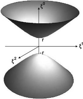
for (namely ), we can rewrite the equation (A.1), defining the quantity , as
which is the equation of an elliptic hyperboloid (see Fig. 7).
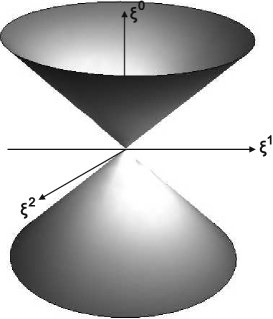
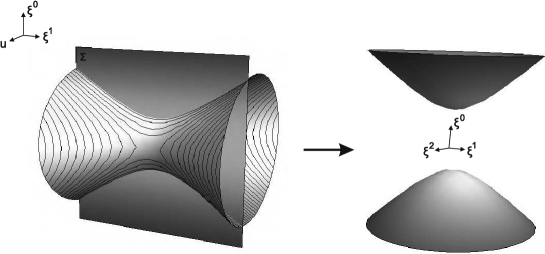
Afterwards, if we take the quantity (namely ), the equation becomes
which is the equation of a cone (see Fig. 8).
Finally, if we take (namely ), the determinant reads
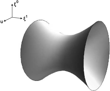
which is the equation of an hyperbolic hyperboloid (see Fig. 9).
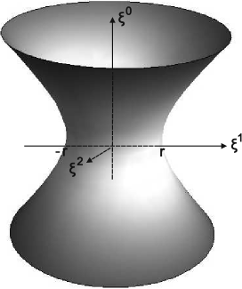
These are all the geometries of the parameter space of the group . In particular, we must imagine that for a fixed value of the parameter , also known as embedding parameter, we generate one of these geometries. We can clarify our ideas observing Fig. 10.
Appendix B Euler coordinates expansion
Starting by the following expression for the group element
in terms of the dimensionful parameters and , we can separate the exponentials as follows
| (B.1) |
this is because , obviously, commutes with itself and then we can divide the exponential in two parts. Now, we focus on the three central exponentials.
Rewriting the latter in matrix form we have
At this point, considering that we defined our spatial momenta as
substituting these expressions we obtain
where the last equality can be easily obtained using the properties of the matrices in the resummation of the exponential. In conclusion, substituting also the Euler angle with our momentum and putting together the exponentials, we obtain the expression (3.3).
Appendix C Change of coordinates between different parametrizations
Let us start by writing all together the set of coordinates on the manifold we considered
| (C.1) |
Now, starting by the system (C.1), we can find the transformation laws from a set of coordinates to another.
C.1 vs
C.2 vs
C.3 vs
Appendix D The Haar measure
Following [18, 23], we can write the Haar measure on in terms of the coordinates which parametrize the group element as
| (D.1) |
where, as always, . In this way we can characterize the Haar measure on for every parametrization.
D.1 Haar measure in Cartesian parametrization
Using the -parametrization we have
is immediate to write the Haar measure on the group; in fact, substituting the parameters in the formula (D.1), we obtain
D.2 Haar measure in exponential parametrization
Using the -parametrization the matter is more complicated. This is because these coordinates appear as a combination of hyperbolic functions
and thus the form of the Haar measure (D.1) is more difficult to obtain. In particular, we have to calculate the determinant of the Jacobian matrix related to the transformation . Performing the calculation, we obtain
which, given equation (D.1), allows us to write the Haar measure as
D.3 Haar measure in Euler parametrization
The Haar measure in the -parametrization can be found in the same way as the previous ones. In particular the new parametrization
leads to the following Jacobian determinant
which implies that the Haar measure in this parametrization is given by
namely
Acknowledgments
We would like to thank the anonymous referees for the insightful comments which helped us improve the paper. MA work is supported by a Marie Curie Career Integration Grant within the 7th European Community Framework Programme and in part by a grant from the John Templeton Foundation.
References
- [1] Agostini A., Amelino-Camelia G., Arzano M., D’Andrea F., A cyclic integral on -Minkowski noncommutative space-time, Internat. J. Modern Phys. A 21 (2006), 3133–3150.
- [2] Agostini A., Amelino-Camelia G., D’Andrea F., Hopf-algebra description of noncommutative-space-time symmetries, Internat. J. Modern Phys. A 19 (2004), 5187–5219, hep-th/0306013.
- [3] Agostini A., Lizzi F., Zampini A., Generalized Weyl systems and -Minkowski space, Modern Phys. Lett. A 17 (2002), 2105–2126, hep-th/0209174.
- [4] Alesci E., Arzano M., Anomalous dimension in three-dimensional semiclassical gravity, Phys. Lett. B 707 (2012), 272–277, arXiv:1108.1507.
- [5] Amelino-Camelia G., Relativity in spacetimes with short-distance structure governed by an observer-independent (Planckian) length scale, Internat. J. Modern Phys. D 11 (2002), 35–59, gr-qc/0012051.
- [6] Amelino-Camelia G., Doubly-special relativity: facts, myths and some key open issues, Symmetry 2 (2010), 230–271, arXiv:1003.3942.
- [7] Amelino-Camelia G., Arzano M., Bianco S., Buonocore R.J., The DSR-deformed relativistic symmetries and the relative locality of 3D quantum gravity, Classical Quantum Gravity 30 (2013), 065012, 17 pages, arXiv:1210.7834.
- [8] Arzano M., Anatomy of a deformed symmetry: field quantization on curved momentum space, Phys. Rev. D 83 (2011), 025025, 12 pages, arXiv:1009.1097.
- [9] Arzano M., Kowalski-Glikman J., Trześniewski T., Beyond Fock space in three-dimensional semiclassical gravity, Classical Quantum Gravity 31 (2014), 035013, 13 pages, arXiv:1305.6220.
- [10] Baez J.C., Wise D.K., Crans A.S., Exotic statistics for strings in 4D BF theory, Adv. Theor. Math. Phys. 11 (2007), 707–749, gr-qc/0603085.
- [11] Bais F.A., Muller N.M., Topological field theory and the quantum double of , Nuclear Phys. B 530 (1998), 349–400, hep-th/9804130.
- [12] Bais F.A., Muller N.M., Schroers B.J., Quantum group symmetry and particle scattering in -dimensional quantum gravity, Nuclear Phys. B 640 (2002), 3–45, hep-th/0205021.
- [13] Baratin A., Dittrich B., Oriti D., Tambornino J., Non-commutative flux representation for loop quantum gravity, Classical Quantum Gravity 28 (2011), 175011, 19 pages, arXiv:1004.3450.
- [14] Baratin A., Oriti D., Group field theory with noncommutative metric variables, Phys. Rev. Lett. 105 (2010), 221302, 4 pages, arXiv:1002.4723.
- [15] Deser S., Jackiw R., ’t Hooft G., Three-dimensional Einstein gravity: dynamics of flat space, Ann. Physics 152 (1984), 220–235.
- [16] Freidel L., Livine E.R., 3D quantum gravity and effective noncommutative quantum field theory, Phys. Rev. Lett. 96 (2006), 221301, 4 pages, hep-th/0512113.
- [17] Freidel L., Majid S., Noncommutative harmonic analysis, sampling theory and the Duflo map in quantum gravity, Classical Quantum Gravity 25 (2008), 045006, 37 pages, hep-th/0601004.
- [18] Fuchs J., Schweigert C., Symmetries, Lie algebras and representations. A graduate course for physicists, Cambridge Monographs on Mathematical Physics, Cambridge University Press, Cambridge, 1997.
- [19] Guedes C., Oriti D., Raasakka M., Quantization maps, algebra representation, and non-commutative Fourier transform for Lie groups, J. Math. Phys. 54 (2013), 083508, 31 pages, arXiv:1301.7750.
- [20] Joung E., Mourad J., Noui K., Three dimensional quantum geometry and deformed symmetry, J. Math. Phys. 50 (2009), 052503, 29 pages, arXiv:0806.4121.
- [21] Koornwinder T.H., Muller N.M., The quantum double of a (locally) compact group, J. Lie Theory 7 (1997), 101–120, q-alg/9605044.
- [22] Majid S., Schroers B.J., -deformation and semidualization in 3D quantum gravity, J. Phys. A: Math. Theor. 42 (2009), 425402, 40 pages, arXiv:0806.2587.
- [23] Matschull H.-J., Welling M., Quantum mechanics of a point particle in -dimensional gravity, Classical Quantum Gravity 15 (1998), 2981–3030, gr-qc/9708054.
- [24] Meljanac S., Samsarov A., Stojić M., Gupta K.S., -Minkowski spacetime and the star product realizations, Eur. Phys. J. C 53 (2008), 295–309, arXiv:0705.2471.
- [25] Meljanac S., Škoda Z., Svrtan D., Exponential formulas and Lie algebra type star products, SIGMA 8 (2012), 013, 15 pages, arXiv:1006.0478.
- [26] Noui K., Three-dimensional loop quantum gravity: towards a self-gravitating quantum field theory, Classical Quantum Gravity 24 (2007), 329–360, gr-qc/0612145.
- [27] Sasai Y., Sasakura N., The Cutkosky rule of three dimensional noncommutative field theory in Lie algebraic noncommutative spacetime, J. High Energy Phys. 2009 (2009), no. 6, 013, 22 pages, arXiv:0902.3050.
- [28] Sasai Y., Sasakura N., Massive particles coupled with dimensional gravity and noncommutative field theory, arXiv:0902.3502.
- [29] Schroers B.J., Lessons from -dimensional quantum gravity, PoS Proc. Sci. (2007), PoS(QG–PH), 035, 15 pages, arXiv:0710.5844.
- [30] Schroers B.J., Wilhelm M., Towards non-commutative deformations of relativistic wave equations in dimensions, SIGMA 10 (2014), 053, 23 pages, arXiv:1402.7039.
- [31] Staruszkiewicz A., Gravitation theory in three-dimensional space, Acta Phys. Polon. 24 (1963), 735–740.
- [32] ’t Hooft G., Quantization of point particles in -dimensional gravity and spacetime discreteness, Classical Quantum Gravity 13 (1996), 1023–1039, gr-qc/9601014.
- [33] Welling M., Two-particle quantum mechanics in gravity using non-commuting coordinates, Classical Quantum Gravity 14 (1997), 3313–3326, gr-qc/9703058.