Encapsulating Formal Methods within Domain Specific Languages:
A Solution for Verifying Railway Scheme Plans

Abstract

The development and application of formal methods is a long standing research topic within the field of computer science. One particular challenge that remains is the uptake of formal methods into industrial practices. This paper introduces a methodology for developing domain specific languages for modelling and verification to aid in the uptake of formal methods within industry. It illustrates the successful application of this methodology within the railway domain. The presented methodology addresses issues surrounding faithful modelling, scalability of verification and accessibility to modelling and verification processes for practitioners within the domain.

1. Introduction

Formal methods in software engineering have existed at least as long as the term “software engineering” itself, which was coined at the NATO Science Conference, Garmisch, 1968. In many engineering-based application areas, such as in the railway domain, formal verification processes have reached an impressive level of maturity as demonstrated by various industrial case studies, e.g. see [4, 45, 46, 40, 15]. Authors like Barnes also demonstrate that formal methods can be cost effective [1]. Even though these studies successfully illustrate the use of formal methods from an academic perspective, adoption of formal methods within industry is still limited [5]. From the industrial perspective, issues include

Faithful modelling:

Do the proposed mathematical models faithfully represent the systems of concern? Modelling approaches offered from computer science are often in a form that is acceptable to computer scientists, but not to the engineer working within the domain. How can an engineer working within the domain come up with new models?

Scalability:

Does the proposed technology scale up to industrially sized systems in a manner that is uniformly applicable? Often, formal methods have been applied in a pilot to specific systems, but require individual, hand-crafted adaptation and optimisation for each new system under consideration.

Accessibility:

Are the methods accessible to practitioners in the domain of interest or is it just the developers of the approach who can apply them? Handling of tools for verification procedures is often aimed towards a computer science audience specialised in verification, however they are usually not manageable by engineers outside the field of formal methods.

This paper presents a new methodology addressing these three issues. The underlying theme is that

“Domain Specific Languages (DSLs) can aid with modelling, verification and encapsulation of formal methods tools within a given domain”.

We first present our methodology in general terms and then demonstrate it on the concrete example of verifying scheme plans from the railway domain. Our methodology is centered around the algebraic specification language Casl [37]. Casl provides us with a sound semantic foundation. Furthermore, Casl offers mature tool support for verification. Our methodology takes as a starting point industrial documents describing a DSL, see for instance the Invensys Rail Data Model [12]. We then stepwise develop a modelling and automated verification process. Thanks to elements such as graphical tooling, the process as a whole is accessible to practitioners in the domain, verification is scalable, and models are guaranteed to be faithful.

The paper is organised as follows: First, we discuss our methodology in detail. Then, we introduce railway signalling as the domain in which we demonstrate our methodology and present the DSL which will serve as running example throughout the paper. The next sections apply the methodology step by step: in Section 4 we give a method for formalising a DSL within Casl (Step M1); Section 5 demonstrates how to exploit implicit domain knowledge for the purpose of verification (Step M2); Section 6 presents techniques to encapsulate formal methods within a tooling framework (Step M3) – this includes the presentation of competitive verification results for railway scheme plan verification. Finally, we place our work in context by discussing related work.

While in the context of this paper we deal with an “academic” DSL, it is worth noting that we have successfully, i.e., with the same positive results, applied our methodology to the DSL [12] of our industrial partner – see [16]. The chosen academic language is of smaller extent, however, it “covers” all challenging elements.

As the paper covers such diverse topics as railways, modelling in Casl, verification, and tooling, we present their respective background distributed over the paper. We use the labels “background” and “contribution” to signpost the status of each subsection. Our paper is based upon the PhD thesis of the first author [16] and earlier results on the topic. Complete specifications, further details and further examples for the work we present in this paper can be found in the thesis [16]. In 2011, we published a first version of our methodology [22]. In 2012, we gave a first report upon the exploitation of domain knowledge for verification [17]. In 2013, we discussed in detail how to formalise DSLs within Casl [19]. However, this paper comprises the first complete presentation of the whole methodology.

2. A Methodology for Encapsulating Formal Methods within DSLs

We begin by introducing the topic of domain specific languages (DSLs), paying particular attention to the common industrial representation used to formulate such languages in terms of UML class diagrams accompanied by a narrative. For such industrial DSLs, we then develop our methodology in a detailed step-by-step manner.

2.1. Background: Domain Specific Languages (DSLs)

Throughout all areas of science, one can find approaches that are general in principle or specific to the task at hand. A general approach gives a solution to several problems of a similar manner. Whereas a specific approach often solves problems in a more comprehensive manner, but can be applied to significantly less problems. In computer science, the differences are exemplified by general purpose languages (GPLs) and domain specific languages (DSLs) respectively.

Domain specific languages (DSLs) [29], are languages that have been designed and tailored for a specific application domain. DSLs aim to abstract away technical details of computer science from the user, allowing them to create programs or specifications without having to be an expert programmer or specifier. Examples of DSLs include the well known Backus Naur Form or the commonly used HTML markup language. Considering HTML, it is designed explicitly with webpage creation in mind. It has specific features such as elements, tags and attributes that allow the specification of structure within a web page. The advantages of having these domain specific features are apparent as HTML has become the de facto standard for webpage creation thanks to its expressiveness and to its ease of application. When we speak of expressiveness in the context of DSLs, we refer to the question of how easy it is for a user to describe the objects they desire. Expressiveness can often be explored by considering how intuitive various language constructs are. This idea forms a main theme throughout this work.

2.1.1. DSLs Formulated using UML Class Diagrams and Narrative

UML Class Diagrams [38] are industrially accepted for modelling a variety of systems across numerous domains. Often they are used to describe all elements and relationships occurring within a domain. As such, a UML Class Diagram can be thought of as describing a DSL. Many tools and frameworks actually use UML class diagrams as a starting point for the description of a DSL [9, 27]. A typical example of such an endeavour is given by the Data Model [12] of our research partner Invensys Rail. It aims to describe all elements within the railway domain.

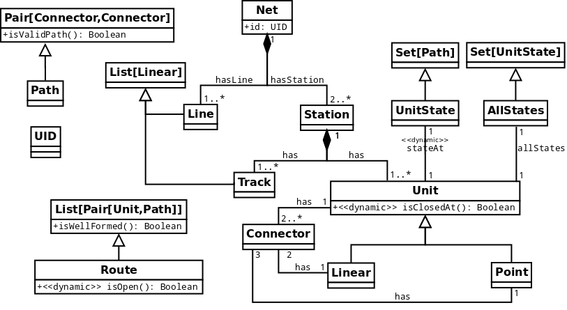
Figure 1. Part of Bjørner’s DSL captured in a UML Diagram.

The UML diagram in Figure 1 captures Bjørner’s railway DSL [2] that we will use as a running example. It illustrates many of the features of class diagrams:

• Classes, represented by a box, e.g. Net, Unit, Station etc. These represent concepts from the railway domain.

• Properties, listed inside a class, e.g. id : UID in the class Net expresses that all Nets have an identifier of type UID.

• Generalisations, represented by an unfilled arrow head, e.g. Point and Linear are generalisations of Unit.

• Associations, represented by a line connecting two classes, e.g. the has link between Unit and Connector. These can have direction, and also multiplicities associated with them. The multiplicities on the has association between Unit and Connector can be read as: “One Unit has two or more connectors”.

• Compositions, represented by a filled diamond, e.g. the hasLine composition for Net and Line, tell us that one class “is made up of” another class. In a similar fashion to associations, compositions can also have multiplicities.

• Operations are also represented inside a class, e.g. the isOpen operation of type Boolean inside the Route class.

As UML class diagrams only capture static system aspects, we make the realistic assumption that the class diagram is accompanied with some narrative. Obviously, such a narrative can give explanations on the static structure of the class diagram. Its main purpose, however, is to describe the dynamic system aspects. For many domains such a narrative is present in the form of standard literature. An example of this is Kerr’s narrative for the railway domain [26]. Kerr describes, for instance, how a signal changes using the following narrative: ”a repeater signal shows yellow if its parent signal is showing red” [26]. Further examples of narrative are N1 and N2 in Section 3.1.

UML class diagrams and narratives can be linked via the stereotype dynamic. This annotation indicates that the labelled class diagram element element is related to the dynamic nature of the system. The manner in which change happens is described in the narrative. In Figure 1, e.g., the relation stateAt is marked to be of dynamic nature, i.e., to change over time. Section 3 provides the narrative how this state change happens.

2.2. Contribution: The Design Steps of our Methodology

To achieve a faithful, scalable and accessible modelling and verification procedure, we present a new methodology that encapsulates formal methods within a DSL. This results in a tool based framework for verification.

Considering Figure 2, the encapsulation process we propose is undertaken by a team comprising of computer scientists working in close collaboration with experts from the domain. Here, the close working relationship ensures the resulting domain modelling is faithful. The following steps are involved in the process:

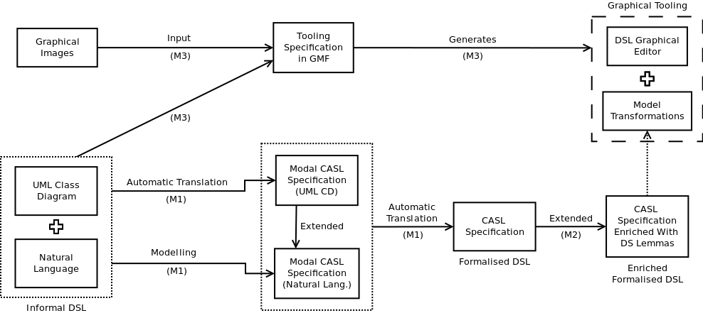
Figure 2. The proposed methodology.

M1: Formalising (Industrial) DSLs

The starting point for our methodology is an informal domain description in the form of UML Class Diagrams and accompanying narrative. From such UML class diagrams, names, relations, and multiplicity constraints can be automatically extracted and translated into a formal specification in ModalCasl. We suggest and support a particular automatic translation (see Section 4.2). Next, domain experts and computer scientists extend the resulting formal ModalCasl specification with a modelling of the narrative that captures dynamics. This is possible as ModalCasl allows the description of state changes in terms of modal operators. Here, we also encode proof goals for verification. Then, for the sake of better proof support, we apply an existing automatic translation from ModalCasl to Casl. Overall, starting from an existing DSL and involving domain experts ensures a faithful formalisation of the selected domain concepts.

M2: DSL Analysis for Verification Support

The result of Step M1, the formalisation of the DSL, is a loose Casl specification – see Section 4.1 for details. The logical closure of this specification, i.e., all theorems that one can prove from this Casl specification, is what we call the implicitly encoded “domain knowledge” of the DSL. We make (part of) this domain knowledge explicit in the form of lemmas that allow one to refactor any proof goals into equivalent ones that are expressed on the right level of granularity. Naturally, there cannot be a universal solution to finding such domain specific lemmas. However, in our experience, for all DSLs we have considered, such lemmas have existed, follow from knowledge of the domain experts, and allow refactoring. We discuss such lemmas in Section 5.3 and show that these lemmas allow for scalable verification based on ideas that are often inherent to the domain. Overall, this step enables scalability of the verification approach.

M3: Graphical Tool Support

DSLs are often accompanied by a development framework. For this we make use of the Graphical Modelling Framework, GMF [9]. GMF provides the infrastructure to create, from a UML class diagram, a Java based graphical editor. Using GMF, domain experts and computer scientists create such a graphical tooling environment for the DSL. This allows for native graphical representations of domain elements. Such an editor is open (via Epsilon [27]) to extension with model transformations [27]. Such transformations allow for the graphical models produced by the editor to be translated to Casl specifications. These specifications can be enriched with the domain knowledge developed in Step M2. We illustrate this approach in Section 6.2, giving details of the OnTrack Toolset for the railway domain. The result of this step is a tool for generation of formal models that is readily usable by engineers from the domain under consideration.

2.2.1. Addressing the Issues

Overall, our methodology addresses the issues we started with: faithful modelling is achieved thanks to starting with an informal description and forming a formal specification in a close working relationship between the domain experts and computer scientists; scalability of the verification procedure is achieved thanks to the property supporting domain specific lemmas; accessibility to modelling and verification of systems is achieved thanks to graphical tooling incorporating domain specific concepts and constructs.

2.3. Contribution: The Resulting Verification Process

The result of applying our methodology is a toolset accommodating the verification process illustrated in Figure 3. This process is undertaken purely by the engineers in the domain. It follows three main steps:

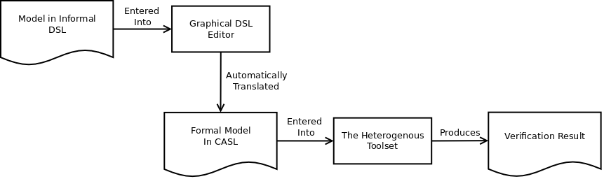
Figure 3. A verification process based on the designed tools.

V1: Model Development Based on the Informal DSL

The first (optional) step within industry is to outline or specify a design informally. This step should be undertaken using the vocabulary outlined within the informal DSL.

V2: Graphical Modelling

Next, the domain engineer can encode their design using the graphical editor. Once encoded, the engineer can automatically produce formal specifications ready for verification. As the graphical editor contains constructs that are from the informal DSL, training and learning costs are minimal.

V3: Verification

Finally, the formal specifications can be verified using (for Casl) the Heterogeneous Toolset, Hets [36]. Due to the domain specific lemmas developed during the design process, verification is automated and “Push Button”.

3. The Railway Signalling Domain

We now introduce the railway signalling domain. We discuss the main elements of this domain and present an established DSL by Bjørner [2] that captures it. Here, we first present the narrative before discussing the UML class diagram.

3.1. Background: Industrial Practice in the Railway Domain

In industry, companies such as our industrial partner, Invensys Rail, undertake domain engineering with the aim to “describe all concepts, components and properties within the railway domain” [12]. This modelling, for example, includes features such as rail topology (the basic graph underlying the railway), dimensions (e.g, where tracks are with regards to reference points, the length of tracks, etc), and signalling (routes, speed restrictions etc.). Common across all these layers is the notion of a track plan as a term to describe layouts of junctions and stations. Track plans combine topological information and the conceptual abstraction of routes, which determine the use of a rail layout. An example track plan is shown in Figure 4.

Route	Clear	Normal	Reverse
RX1	LA1, P1, PLAT1		P1
R1Y	P2, LA2		P2
RX2	LA1, P1, PLAT2	P1
R2Y	P2, LA2	P2

Route	Point(Cleared By)
RX1	P1(P1)
R1Y	P2(LA2)
RX2	P1(P1)
R2Y	P2(LA2)

Figure 4. A scheme plan for a simple station. Top: Track plan, Bottom Left: Control table, Bottom Right: Release table.

The intended operation of the train station shown in Figure 4 is: (1) trains enter at X using track LA1, they then proceed across point P1 towards the upper line to platform PLAT1 (i.e. taking route RX1); (2) alternatively, they pass over point P1 towards the lower line and proceed to platform PLAT2 (i.e. taking route RX2); (3) trains from platform PLAT1 can then pass back the lower line using point P2 and exit the station through track LA2 (i.e. taking route R1Y); (4) finally, trains from platform PLAT2 can pass across point P2 and exit the station through track LA2 (i.e. taking route R2Y).

Such a track plan is usually paired with a set of control and release tables [26] to form a scheme plan – see Figure 4. A scheme plan details the conditions required for route availability. The operational setting and unsetting of points and routes is controlled by an interlocking which is implemented based on this scheme plan.

The control table prescribes that a given route can be used when all tracks in the “clear” column are not occupied by a train, and the points in the “normal” and “reverse” columns are set to those positions. The example control table prescribes that route RX1 can be assigned to a train when units LA1, P1, and PLAT1 are unoccupied and point P1 is in its reverse position, that is, allowing trains to travel to the top line of Figure 4. We note that the track plan in Figure 4 is uni-directional and that if it were bi-directional, there would be routes corresponding to the opposite direction of travel. The rules for these routes would also share tracks with the current rules, stopping the possibility of routes in opposite directions being used at the same time.

The interlocking also allocates so called locks on points to particular route requests. These locks ensure that the point remains locked in position. Such locks are then released according to the information in the release table. For example, the first row of the release table states that for route RX1 the point P1 can be released by the point itself becoming clear. Releasing of these locks allows the corresponding points to be used within another route. Notice, that for a point which splits two routes, i.e. point P1, the lock on the point can be released by the point itself. However, for points that merge two routes, i.e. point P2, there is the added safety check that the point can only be released after the shared parts of the routes are cleared, i.e. track LA2.

Finally, the last element in the dynamic operation of railways is that of train movements. Above, we have described how access to certain routes is granted, and areas of tracks can be released. This follows conventional railway signalling [26]. However, the newer ETCS [8] standard builds on this conventional signalling with the notion of a movement authority. A movement authority can be thought of as an area of railway for which a train can be granted access to travel along. For example, a train may be granted access to move along units LA1 and P1 in Figure 4. The assignment of movement authorities is given by the following narratives:

N1 – Extension:

Initially, no train has a movement authority. A request can be made for a train to travel along a particular route. If the route is available (as dictated by the control table) then the train’s movement authority can be extended to include the route. The movement authority for a train can contain multiple routes.

N2 – Release:

As a train travels it releases regions of railway from its movement authority according to the release table for that route.

Such movement authorities allow the example run illustrated in Figure 5. In the beginning, at time $0$, there is no train in the system. At time $1$, train A has been detected by track circuit $LA1$. Train A travels to platform PLAT1 where it resides until it has been overtaken by train B. Train A then travels further and leaves the system. This run illustrates that train A releases the use of point P1 before it exits the full route RX1. This allows for train B to use route RX2 whilst the end of route RX1 is still in use by train A.

Time	LA1	P1	PLAT1	PLAT2	P2	LA2
0	_	_	_	_	_	_
1	$\Longmapsto_{a}$	_	_	_	_	_
2	_	$\Longmapsto_{a}$	_	_	_	_
3		_	$\Longmapsto_{a}$	_	_	_
4	$\Longmapsto_{b}$	_	$\Longmapsto_{a}$	_	_	_
5	$\_$	$\Longmapsto_{b}$	$\Longmapsto_{a}$	_	_	_
6	$\_$	$\_$	$\Longmapsto_{a}$	$\Longmapsto_{b}$	_	_
7	$\_$	$\_$	$\Longmapsto_{a}$	_	$\Longmapsto_{b}$	_
8	$\_$	$\_$	$\Longmapsto_{a}$	_	_	$\Longmapsto_{b}$
9	$\_$	$\_$	$\Longmapsto_{a}$	_	_	_
10	$\_$	$\_$	_	_	$\Longmapsto_{a}$	_
11	$\_$	$\_$	_	_	_	$\Longmapsto_{a}$
12	_	_	_	_	_	_

Figure 5. A time/position diagram for an example run of the station.

3.1.1. Discussion of Safety Properties

In railway signalling, many different safety properties have been considered. For example, on the concrete level of an interlocking, one may want to check the concrete property that “Signal x only shows green when route y is free to use” [21]. Alternatively, when checking the design of a scheme plan, Moller et al. check that the control table ensures collision-freedom (excluding two trains occupying the same track) [33]. Our aim differs slightly, as we consider the assignment of movement authorities which is outlined by the ETCS standard [8]. Therefore we verify that “overlapping movement authorities are not assigned at the same time”.

Such a property is at a higher level of abstraction than the properties mentioned previously. However, as movement authorities are extended depending on the rules of the control table, we do in fact cover the property of collision freedom under the assumption that trains are well behaved. That is, if trains stay within their given movement authority, and movement authorities are proven to never overlap, then we know two trains cannot occupy the same track unit.

3.2. Background: Bjørner’s DSL Adapted for ETCS

The process of identifying, classifying and precisely defining the elements of a domain has been coined as “Domain Engineering” by Dines Bjørner [3]. Bjørner gives such a classification, i.e., DSL, for the railway domain using a narrative [2] which we introduce as a running example.

Figure 1 shows part of the UML class diagram for Bjørner’s DSL. A railway is a “Net”, built from “Station(s)” that are connected via “Line(s)”. A station can have a complex structure, including “Tracks”, “Switch Points” (also called points) and “Linear Units”. “Tracks” and “Lines” can only contain “Linear Units”. All “Unit(s)” are attached together via “Connector(s)”. Along with defining these concepts, Bjørner stipulates various well-formedness conditions on such a model, for example, “No two distinct lines and/or stations share units.” or “Every line of a net is connected to exactly two, distinct stations” [2].

Bjørner’s approach contains the necessary terms to describe the track plan in Figure 4. The whole track plan forms a station. This station contains all elements such as switch points $P1$ and $P2$ along with linear units $LA1,PLAT1,PLAT2$, and $LA2$, and connectors $c1,c2,\dots,c8$ for connecting these units. From this point on, we only consider the elements of Bjørner’s DSL that we require for modelling track plans we are interested in. Therefore, some of the conditions stipulated by Bjørner do not apply. For example, the track plan given in Figure 4 is open ended. Hence, axioms regarding closed networks, such as the condition “all nets must contain two stations” (leaving no open lines), do not apply to our models.

Bjørner’s DSL gains dynamics by attaching a state to each unit [2]. Each unit can be in one of several states at a given time. A state is represented using a set of paths, where a path is a pair of distinct connectors $(c,c^{\prime})$. A path expresses that a train is allowed to move along a given unit from connector $c$ to connector $c^{\prime}$. To combine a unit and a path across it, Bjørner introduces unit path pairs by forming pairs from units and paths across them. These paths allow one to describe which direction along a unit a train is allowed to travel. Trains are not an explicit part of Bjørner’s DSL. Instead, Bjørner describes the concept of a “Route”, which is a dynamic “window” around a train. Concretely, routes are lists of connected units and paths through them. For example, the route from $X$ to $PLAT1$ of Figure 4 would be captured as the list $[(LA1,(c1,c2)),(P1,(c2,c3)),(PLAT1,(c3,c4))].$ Bjørner stipulates that a route can be dynamically changed over time using a movement function that, for a given time, gives the set of assigned routes. This movement function extends or shrinks a route by adding or removing units at one or both of its ends. Train movements are modelled using this function.

Finally, Bjørner has formalised his narrative in (the algebraic part of) RSL [2]. Here we adopt the Casl specification language rather than RSL. Our formalisation follows in great part Bjørner’s modelling, however, we utilise the Casl features of predicates, subsorting, and structuring in order to obtain a more readable specification text. Our choice of Casl is also due to the greater level of proof support that is available for Casl in the form of the Hets environment [36], and the institutional base for Hets which allows us to describe how to implement a comorphism from UML class diagrams to Casl in Section 4.2. Overall, the CASL models we present capture the narrative in a similar manner to the RSL models presented by Bjørner in [2].

4. Formalizing the Signalling Domain

We now present the formalisation of our DSL in Casl. We introduce Casl and ModalCasl, and discuss an automatic formalisation of UML class diagrams. Finally, we model the railway narrative for movement authorities.

4.1. Background: The Underlying Specification Formalisms

We introduce the relevant background on Casl, ModalCasl and give details on translating ModalCasl to Casl.

4.1.1. CASL

The Common Algebraic Specification Language [37], known as Casl, is a specification formalism developed by the CoFI initiative throughout the late 1990’s and early 2000’s in order to design a Common Framework for Algebraic Specification and Development. Casl has basic, structured, and architectural specifications, of which we consider the first two kinds only.

Roughly speaking, a Casl basic specification consists of a signature made up of sorts, operations, and predicates (declared by means of the keywords sort, op, and pred, respectively), and axioms referring to the signature items. Operations can be partial or total. Furthermore, one may declare a subsort relation on the sort symbols. Axioms are written in first-order logic. Going one step beyond first order logic, Casl also features sort generation constraints for datatypes (keywords generated, free type).

As an example consider the Casl specification in Figure 6 formalising the concept of time. The specification has the name Time. It specifies the sort symbol Time, the constant function symbol $0$, the total function symbol suc from sort Time to sort Time, the partial function symbol pre from sort Time to sort Time and the predicate symbol $\_\_$$<=$$\_\_$ over $\textit{Time}\times\textit{Time}$. The axiom is a first order formula stating that $0$ denotes the smallest element of sort Time.

spec	Time $=$
	sort Time
	ops	$0$ $:$ Time;
		suc $:$	Time $\rightarrow$ Time;
		pre $:$	Time $\rightarrow?$ Time
	pred	$\_\_$$<=$$\_\_$ $:$	Time $\times$ Time
	$\forall$	n $:$ Time $\bullet$	$0$ $<=$	n
end

Figure 6. A basic Casl specification, formalising the concept of time.

A model of a Casl specification is an algebra which interprets sorts as (non empty) sets and operations and predicates as (partial) functions and subsets respectively, in such a way that the given axioms are satisfied. The subsorting relation is reflected by injective coercion functions between the sets interpreting the involved sorts (not by subset inclusion), see [34, 37] for further details. The collection of all these models is called the model class of the specification. It is a speciality of Casl to support loose specification, i.e., to write a specification that has algebras of different “forms” in its model class.

The Casl specification Time of Figure 6 has the naturals with the standard interpretations as its model, i.e., discrete time is a possible model. It also has the non-negative reals as a model, i.e., dense continuous time is a possible model as well. The Casl specification Time is a typical example of a loose specification with algebras of different form: the naturals are countable, while the non-negative reals are not countable.

Besides basic specifications, Casl provides ways of building complex (structured) specifications out of simpler ones (the simplest being basic specifications) by means of various specification-building operations. These include translation, hiding, union, and both free and loose forms of extension. In our presentation we make use of only a few of these, on which we elaborate upon below.

Translations of declared symbols to new symbols are specified by giving lists of ‘maplets’ of the form $old\mapsto new$ (keyword with).

The signature of a union of two specifications is the union of their signatures. Given models over the component signatures, the unique model over the union signature that extends each of these models is called their amalgamation. Clearly, not all pairs of models over component signatures amalgamate. The models of a union (keyword and) are all amalgamations of the models of the component specifications.

Extensions (keyword then) may specify new symbols or merely require further properties of old ones. Extensions can be classified by their effect on the specified model class. For instance, an extension is called implicational (annotation %implies) if the signature and model class remain unchanged. Note that this annotation has no effect on the semantics of a specification: a specifier may use them to express their intentions, tools may use them to generate proof obligations, see Section 5 for further details.

Structured specifications may be named, and a named specification may be generic in the sense that it declares parameters that need to be instantiated when the specification is (re)used. Instantiation is a matter of providing an appropriate argument specification.

The generic specification Pair in Figure 7 has two formal parameters, namely the (non-named basic) specification sort S and the (non-named basic) specification sort T. In the specification InstantiatedPair, both these parameters are instantiated with the specification sort Connector as the actual parameter. This results in a sort Pair[Connector,Connector] representing pairs over the sort Connector. In a final step the signature of the instantiated specification is adjusted by a renaming, namely to rename the operation symbols first and second into c1 and c2.

spec	Pair [sort S][sort T] $=$
	sort	Pair[	S,T]
	ops	first $:$	Pair[	S,T] $\rightarrow$ S;
		second $:$	Pair[	S,T] $\rightarrow$ T;
		pair $:$	S $\times$ T $\rightarrow$	Pair[	S,T]
	$\forall$ s $:$ S;	t $:$ T
	$\bullet$	first(pair(	s, t)) $=$ s
	$\bullet$	second(pair(	s, t)) $=$ t
end
spec	InstantiatedPair $=$
		Pair	[sort Connector][sort Connector]
	with	first $:$	Pair[	Connector,Connector] $\rightarrow$ Connector $\mapsto$ c1,
		second $:$	Pair[	Connector,Connector] $\rightarrow$ Connector $\mapsto$ c2
end

Figure 7. A generic Casl specification and its instantiation.

4.1.2. Modal CASL

ModalCasl [35] is an extension of Casl with concepts from Modal Logic. We use only a small sublanguage of ModalCasl described below.

Roughly speaking, a ModalCasl basic specification consists of a signature that is a Casl signature in which operation and predicate symbols can be declared to have a fixed interpretation in all worlds (keywords rigid) or to possibly change interpretation with regards to worlds (keyword flexible). Ordinary operation and predicate declarations are treated as rigid. ModalCasl axioms are Casl axioms extended by first-order logic formulae involving the modal operators $\Diamond$ (“there exists a reachable world such that”) and $\Box$ (“in all reachable worlds holds”).

A model of a ModalCasl specification consists of a set of worlds $W$, one of which is distinguished as the initial one, a binary accessibility relation on $W$, and for each world $w$ a Casl model $M_{w}$, such that carrier sets and the interpretation of rigid operation and predicate symbols are the same for all $M_{w}$, and the given axioms are satisfied. Again, the collection of all these models is called the model class of the specification.

Finally, the Casl specification-building operations carry over to ModalCasl [35].

4.1.3. Translating from Modal CASL to CASL

It is possible to define a semantics preserving map, mathematically speaking a so-called institution comorphism, from ModalCasl to Casl. Given the signature of the ModalCasl specification, one adds a sort $W$ (for “worlds”), a constant $init:W$ and a binary predicate $R:W\times W$ for reachability between worlds; rigid operation and predicate symbols are kept unchanged; for flexible operation and predicate symbols, $W$ is added as an extra argument. Axioms are translated as expected, where $\Diamond$ and $\Box$ are expressed via suitable quantification over $W.$

4.2. Contribution: Automatic Translation of UML Class Diagrams to CASL

The details of our automatic translation are given in [19]. Mathematically it is based on institution theory. In [19] we present a formal semantics to UML class diagrams, extending prior work by Cengarle and Knapp [6]. We then define a semantics preserving translation to ModalCasl. In this paper, we discuss the resulting ModalCasl and show how to formalise the narrative of our DSL.

4.2.1. Translating Bjørner’s DSL to Modal CASL

We consider the result of translating the UML class diagram in Figure 1 along the co-morphism defined in [19].

First, classes from the class diagram are translated to ModalCasl sorts. Generalisations are translated to subsorts in ModalCasl. Note that as part of our translation, we often include and (possibly) instantiate specifications from the Casl Basic Datatypes for the built-in types from the class diagram, e.g. for type formers such as $\mathsf{Pair}[c_{1},c_{2}]$. Considering Bjørner’s DSL we gain the following Casl specification for the translations of classes and generalisations:

%% Classes:
sorts	Net, Station, Unit, …, UID
%% Hierarchy:
sorts	Point, Linear $<$ Unit; …;	Route $<$ ListPairUnitPath

Next, property declarations of the class diagram are translated to total functions. For these functions, the classification into “rigid” and “flexible” are obtained directly from the stereotypes in the class diagram. Thus, we obtain:

%% Properties:
rigid op	id $:$	Net $\rightarrow$? UID
flexible ops isClosedAt $:$	Unit $\rightarrow?$ Boolean;
…

ModalCasl predicates are then used to capture the composition and association declarations. Again, rigid and dynamic elements can be taken from the stereotypes of the class diagram. As well as these, a predicate $\mathit{isAlive}$ is added for each sort. These predicates are used to model “flexible” sort interpretations in ModalCasl, see [19] for details. Considering the running example, we obtain the following ModalCasl:

%% Compositions:
rigid preds $\_\_$has$\_\_$ $:$	Station $\times$ Unit; $\_\_$has$\_\_$ $:$	Station $\times$ Track;
…
%% Associations:
rigid preds $\_\_$has$\_\_$ $:$	Unit $\times$ Connector; $\_\_$has$\_\_$ $:$	Linear $\times$ Connector; …
…
%% Is Alive preds:
rigid preds isAlive $:$ Net; isAlive $:$ Station; isAlive $:$ Unit; …; isAlive $:$ UID;

Finally, we add axioms capturing multiplicity constraints from the class diagram. These can be systematically encoded in first order logic using “poor man’s counting”, by providing the necessary number of variables. A typical example of the mapping for a composition constraint from Bjørner’s DSL is for the composition “Station has Unit”. Where, considering Figure 1 we can see that there must be at least one Unit for every Station. The resulting ModalCasl axiom for this would be:

$\bullet$

$\forall$ s $:$ Station $\bullet$

$\exists$ u $:$ Unit $\bullet$ has(

$s$,

$u$).

Similarly, an example of a constraint on an association is the “has” association between Units and Connectors, where we can see that each Unit must have at least $2$ Connectors. The resulting ModalCasl axiom for this would be:

$\bullet$

$\forall$ u $:$ Unit $\bullet$

$\exists$ c1, c2 $:$ Connector $\bullet$ $\neg$ (

c1 $=$ c2) $\wedge$ has(

$c1$,

$u$) $\wedge$ has(

$c2$,

$u$).

4.2.2. Translating Modal CASL to CASL

Finally, for the sake of better proof support, we apply the existing ModalCasl to Casl comorphism to gain a Casl specification. For example, we add the sort Time to deal with modalities:

sorts

Time, Net, Station, Unit, …, UID

Subsort relations simply remain the same. Similarly, rigid operations and predicates also remain the same:

op

id $:$

Net $\rightarrow$? UID

whilst flexible operations and predicates have the sort Time added to their profile:

op isClosedAt $:$

Unit $\times$ Time $\rightarrow?$ Boolean;

Finally, we note that as the presented examples of axioms for multiplicity constraints are not dependent on flexible operations or predicates, they remain unchanged.

4.3. Contribution: Modelling of the Narrative in CASL

It is a matter of choice which specification language to use to model the dynamic system aspects: in ModalCasl or in Casl. Here, for the sake of readability, we present this modelling in Casl. We note that, throughout the presentation, we have specialised the sort Time gained from applying our comorphism, to the specification given in Figure 6.

4.3.1. Introducing Regions for Movement

To allow us to correctly model the extension and release of movement authorities, we introduce the notion of a region. Regions will allow areas of a track to be reserved and released. Such regions are categorised by both the topological routes of a track plan, and the release points of the release table. For example, considering the pass through station in Figure 4, we can split the topological routes at the units outlined by the release table to gain the possible regions of the scheme plan shown in Figure 8.

Figure 8. Regions of the simple station.

The regions are defined using the release points within the release table to break up a route at the given release unit. To compute the regions of a given route $r$ we define the function $Regions:List[Unit]\times List[Unit]\rightarrow Set[List[Unit]]$ as:

$Regions([u_{1},\dots,u_{n}],[])$ $=$ $\{[u_{1},\dots,u_{n}]\}$ $Regions([u_{1},\dots,u_{n}],[r_{1},r_{2},\dots,r_{m}])$ $=$ $\{[u_{1},\dots,u_{k}]\}\;\cup$ $Regions([u_{k+1},\dots,u_{n}],[r_{2},\dots,r_{m}])$ where $u_{k}=r_{1}$.

We then define the regions of the given route $r$ to be

$$regions(r)=Regions(units(r),releaseTable(r))$$

where $units(r)$ is the list of units occurring within the topological route and $releaseTable(r)$ is the topologically ordered list of release units occurring in the release table for route $r$. For example, considering Figure 8 and the route $RX1$, we have: $Regions([LA1,P1,PLAT1],[P1])=\{[LA1,P1]\}\;\cup\;Regions([PLAT1],[])=\{[LA1,P1],[PLAT1]\}.$ Notice that as we only apply this function to routes and their release tables, each $r_{i}$, for $1\leq i\leq m,$ is guaranteed to occur only once within the list $u_{1},u_{2},\dots,u_{n}$. That is, the region split points will be unique for that route.

Regions allow one to model the interlocking behaviour while taking into account the release tables. As an example, we can see that region $RG1$ contains all the units of routes $RX1$ and $RX2$ up to and including the release point for $P1$ as given by the release table. Then after this release point we gain regions $RG2$ and $RG3$ representing the remaining units from the routes respectively. Such an approach allows, the train movements given in Figure 5 to be captured as the series of region assignments as given in Figure 9.

Time	Train A Movement Authority	Train B Movement Authority
0	$\{\}$	$\{\}$
1	$\{RG1,RG2\}$	$\{\}$
2	$\{RG1,RG2\}$	$\{\}$
3	$\{RG2\}$	$\{\}$
4	$\{RG2\}$	$\{RG1,RG3\}$
5	$\{RG2\}$	$\{RG1,RG3\}$
6	$\{RG2\}$	$\{RG3\}$
7	$\{RG2\}$	$\{RG4\}$
8	$\{RG2\}$	$\{RG4\}$
9	$\{RG2\}$	$\{\}$
10	$\{RG4\}$	$\{\}$
11	$\{RG4\}$	$\{\}$
12	$\{\}$	$\{\}$

Figure 9. Modelling movement with regions.

To model such regions in Casl, we instantiate a specification List with the sort Unit from Bjørner’s DSL. We then define a subsort of these lists called Region. Similarly, we capture movement authorities by instantiating the specification of List with these regions and making a subsort MA:

	List[sort Unit] then	List[sort Region] then
sort	Region $<$	List[Unit]
sort	MA $<$	List[Region]

Next, according to the rules for movement authorities given in Section 3.1, we model the assignment of a movement authority at a given time as a predicate assigned $:$ MA $\times$ Time. That is, if a train is assigned a movement authority then it is allowed to travel along the railway elements contained within the movement authority. We then add an axiom that states that only an empty movement authority can be assigned initially, that is at time $0$:

pred	assigned $:$	MA $\times$ Time
$\bullet$	$\forall$ m $:$ MA $\bullet$	$\neg$	m $=$	$[$$]$ $\Rightarrow$ $\neg$ assigned(	m, $0$) %(no$\_$ma$\_$0)%

Similarly, to model the fact that a train can be granted a movement authority at any time, we add an axiom that states the empty movement authority is always available for extension:

$\bullet$

$\forall$ t $:$ Time $\bullet$ assigned(

$[$$]$ as MA, t) %($[$$]$_assigned_at_ all_times)%

We then add an axiom that states when the predicate assigned can hold for non empty lists. To simplify the definition, we make use of predicates canExtend $:$ MA $\times$ Time and canReduce $:$ MA $\times$ Time whose definitions we discuss next. The axiom given below allows for movement authorities at some time $suc(t)$ to remain assigned as they were at time $t$, become extended from time $t$ and also to reduce from time $t$. It also states that only for one of these possibilities can occur for a given movement authority at a given time. This definition matches the expected behaviour of movement authorities given above.

	$\bullet$	$\forall$ ma1 $:$ MA; t $:$ Time
		$\bullet$	$\neg$	ma1 $=$	$[$$]$ $\Rightarrow$	assigned(	ma1, suc(t))
				$\Rightarrow$	(	assigned(	ma1, t) $\wedge$ $\neg$ canExtend(	ma1, t) $\wedge$ $\neg$ canReduce(	ma1, t))
					$\vee$ (	$\neg$ assigned(	ma1, t) $\wedge$ canExtend(	ma1, t) $\wedge$ $\neg$ canReduce(	ma1, t))
					$\vee$ (	$\neg$ assigned(	ma1, t) $\wedge$ $\neg$ canExtend(	ma1, t) $\wedge$ canReduce(	ma1, t))
%(assigned_defn)%

The predicate canExtend $:$ MA $\times$ Time is true for a given movement authority $ma2$, at a time $t$, when the following conditions are met: (1) there exists a movement authority $ma1$ and a route $r$ such that the movement authority $ma1$ is assigned at $t$ and can be extended to $ma2$ by route $r$. Here, the topological information of valid extensions from the track plan are encoded using the predicate ext $:$ MA $\times$ Route $\times$ MA. We control the behaviour of this predicate by adding the following axiom:

$\bullet$

ext(

ma1, r, ma2) $\Rightarrow$

ma2 $=$

ma1 $++$ regions(r) %(ext$\_$defn)%

stating that ext behaves like list concatenation. (2) The route used for the extension is open at the given time – where the predicate $\_\_$isOpenAt$\_\_$ $:$ Unit $\times$ Time is used (as we shall see later in Section 4.3.2) to encode the clear table conditions of a route; (3) If the movement authority that is being extended is non empty, it becomes not assigned. This is encoded in Casl as:

$\forall$ ma1 $:$ MA;	t $:$ Time
$\bullet$	canExtend(	ma1, t)
	$\Leftrightarrow$	$\exists$ ma2 $:$ MA; r $:$ Route
		$\bullet$	assigned(	ma2, t) $\wedge$ ext(	ma2, r, ma1)
			$\wedge$	r isOpenAt t $\wedge$ (	$\neg$	ma2 $=$	$[$$]$ $\Rightarrow$ $\neg$ assigned(	ma2, suc(t))) %(extends_defn)%

In a similar manner, the predicate canReduce $:$ MA $\times$ Time is true at a given time $t$ for a given movement authority $ma1$ if there exists a region $rg$ such that the movement authority with the region in front of $ma1$ was assigned at $t$ and becomes unassigned at $suc(t)$.

$\forall$ ma1 $:$ MA;	t $:$ Time
$\bullet$	canReduce(	ma1, t)
	$\Leftrightarrow$	$\exists$ rg $:$ Region
		$\bullet$	assigned(	(	rg $::$ ma1) as MA, t) $\wedge$ $\neg$ assigned(	(	rg $::$ ma1) as MA, suc(t)) %(reduces_defn)%

Finally, we would like to ensure that only one movement authority can be extended at any given time, this is captured using the following axiom:

$\bullet$	$\forall$ t $:$ Time
	$\bullet$	$\forall$ m1, m2 $:$ MA
		$\bullet$	(	assigned(	m1, suc(t)) $\Rightarrow$ canExtend(	m1, t)) $\wedge$
				(	assigned(	m2, suc(t)) $\Rightarrow$ canExtend(	m2, t))
			$\Rightarrow$	m1 $=$ m2%(one_MA_changes)%

This assumption is justified by the fact that the Invensys railway control systems, which are responsible for one rail node, handle at most one route request at a given time.

4.3.2. Modelling Control Tables and Route Availability

The above modelling of movement authorities requires the definition of what it means for a route to be open. As we have seen, this information is given by the control table. To model a control table, we introduce the predicate clear $:$ Route $\times$ Unit. We then use this predicate to encode that a particular unit occurs within the clear column for the given route. The control table given in Figure 4 would be encoded as:

$\bullet$ clear(	RX1, LA1)
$\bullet$ clear(	RX1, P1)
…
$\bullet$ clear(	RX2, LA2)

In a similar manner, we could use predicates to encode the normal and reverse columns of the control table. This would be a straight-forward extension of our railway model. However, we we refrain from this as we use the railway domain only as a proof of concept. Therefore, we assume from now on that the normal and reverse columns in the control table are correct. Consequently, we exclude their definitions in our modelling. Using the above described predicates we give the following definition of what it means for a route to be open:

$\forall$ r $:$ Route;

t $:$ Time $\bullet$

r isOpenAt t $\Leftrightarrow$

$\forall$ u $:$ Unit $\bullet$

clear(

r, u) $\Rightarrow$

u isOpenAt t

This axiom states that a route $r$ is open at a given time $t$ if for all units $u$ for which clear($r,u$) holds, the unit $u$ is open at $t$.

Finally, we have yet to consider what is means for a unit to be occupied. Within the operation of an interlocking a unit is in use when a train is detected on a particular track. In our modelling, we abstract on the concrete position of a train and instead say that if a region is assigned to some train, then we assume that the interlocking knows that the region is assigned. We model this by saying that one of the units of the region is not open for use. This is captured by the following axiom:

$\bullet$	$\forall$ t $:$ Time; r $:$ Route; rg $:$ Region; ma $:$ MA
	$\bullet$ assigned(	ma, t) $\wedge$	rg eps regions(r) $\wedge$	rg eps ma
	$\Rightarrow$	$\exists$ u $:$ Unit; upp $:$ UnitPathPair
		$\bullet$ $\neg$	u isOpenAt t $\wedge$	u eps rg $\wedge$	getUnit(upp) $=$ u $\wedge$	upp eps r %(occupied)%

This axiom makes use of the operation regions $:$ Route $\rightarrow$ MA that, for a given route gives the regions it has been split into via our modelling. It also make use of the operation eps that simply stands for elementhood. That is, it captures that region $r$ “is in” movement authority $ma$. Overall, the axiom links the assignment of a movement authority to the openness of a units within the movement authority. Although this axiom is fairly loose, i.e. we do not even impose the restriction that trains should move in the correct direction, this is enough to prove the safety property we discuss next.

4.3.3. Modelling our Safety Property

In Section 3.1.1 we discussed the safety property that we would like to verify. To model such a property, we introduce the auxiliary predicate share $:$ MA $\times$ MA that encodes what it means for two movement authorities to overlap:

pred	share $:$	MA $\times$ MA
	$\forall$ ma1, ma2 $:$ MA
		$\bullet$	share(	ma1, ma2) $\Leftrightarrow$	$\exists$ rg $:$ Region $\bullet$	rg eps ma1 $\wedge$	rg eps ma2 %(share_defn)%

This allows us to model safety using the following formula:

$\forall$ t $:$ Time, ma1, ma2 $:$ MA
	$\bullet$	share(	ma1, ma2)
	$\Rightarrow$	ma1 $=$ ma2 $\vee$ $\neg$ (	assigned(	ma1, $t$) $\wedge$ assigned(	ma2, $t$)) %(safety)%

It states that if two movement authorities share a region, then either they are the same, or they are never both assigned at the same time. This concludes our modelling for movement authorities and safety, next we consider supporting verification of such a property.

5. Automating Verification for the Signalling Domain

We now consider the task of verifying our safety property over models formulated using our formal DSL. We begin by introducing the proof support that is available for Casl. We then show that verification is only possible thanks to exploitation of domain specific lemmas that we introduce thanks to domain knowledge.

5.1. Background: Theorem Proving for CASL

With respect to Casl and ModalCasl, tool support comes in the form of Hets [36], the Heterogeneous Tool Set. Hets supports parsing (is the specification correct w.r.t. the context-free grammar?) and static analysis (is the specification correct w.r.t. context-sensitive properties, such as: have all sorts occurring in a formula been declared?) of specifications written in Casl and ModalCasl. Hets also acts as a broker to various proof assistants and automated theorem provers that can be called to discharge proofs. We mainly make use of SPASS [44] and of eProver [42] both of which support theorem proving for first-order logic with equality. At this point, we note that in our experience with our models, both these theorem provers work best with smaller axiomatic bases. Hence whenever possible, we make our specifications as loose as possible by systematically excluding axioms that are not required for a given proof.

5.2. Contribution: Unsuccessful Verification Over Bjørner’s DSL

Overall, the capturing of Bjørner’s DSL along with our extension of movement authorities in Casl is straightforward. However, with respect to verification, both SPASS and eProver were unable to directly prove our safety property (within six hours each). Even with the addition of the following property specific axiom for induction over time, both provers still fail:

$\bullet$ (	$\forall$ ma1, ma2 $:$ MA $\bullet$	share(	ma1, ma2)
	$\Rightarrow$	ma1 $=$ ma2 $\vee$ $\neg$ (	assigned(	ma1, $0$) $\wedge$ assigned(	ma2, $0$))) %(base case)%
	$\wedge$
	$\forall$	t $:$ Time $\bullet$	(	$\forall$ ma1, ma2 $:$ MA $\bullet$	share(	ma1, ma2)
		$\Rightarrow$	ma1 $=$ ma2 $\vee$ $\neg$ (	assigned(	ma1, t) $\wedge$ assigned(	ma2, t)))
	$\Rightarrow$ (	$\forall$ ma1, ma2 $:$ MA $\bullet$	share(	ma1, ma2)
		$\Rightarrow$	ma1 $=$ ma2 $\vee$ $\neg$ (	assigned(	ma1, suc(t)) $\wedge$ assigned(	ma2, suc(t)))) %(step case)%
$\Rightarrow$ $\forall$	t $:$ Time $\bullet$	(	$\forall$ ma1, ma2 $:$ MA $\bullet$	share(	ma1, ma2)
	$\Rightarrow$	ma1 $=$ ma2 $\vee$ $\neg$ (	assigned(	ma1, t) $\wedge$ assigned(	ma2, t)))

This is not surprising, as we, as well as Bjørner, have intended to provide a strong language for modelling, and we have aimed to model movement authorities intuitively. However, the concept of a movement authority and our safety principle lend themselves, on the general level of the railway domain, to natural abstraction that we now show can be exploited for verification.

5.3. Contribution: Developing DSL Specific Knowledge

Within the railway domain, it is understood that control tables are vital in ensuring safety. In our presentation we can see that movement authorities are extended depending on the rules of the control table. That is, for a movement authority to be extended by the regions of a route, that route must be open. Through domain analysis, we can reduce the reasoning on the level of movement authorities, to a reasoning on the level of topological routes and the control table. This is captured by following domain specific lemma:

Lemma 1 (Property Reduction to Routes).

Given a scheme plan $SP$ then

$\forall$ t $:$ Time; m1, m2 $:$ MA $\bullet$ share(m1, m2)
	$\Rightarrow$ m1 $=$ m2 $\vee$ $\neg$ (assigned(m1, $t$) $\wedge$ assigned(m2, $t$)) %(*)%

if and only if,

$\forall$ t $:$ Time; r $:$ Route; rg $:$ Region; ma $:$ MA
	$\bullet$ assigned(ma, t) $\wedge$ rg eps ma $\wedge$ rg eps regions(r)
		$\Rightarrow$ $\neg$ r isOpenAt t %(**)%

The proof follows by induction on time from the axioms we have presented, including the induction axiom of Section 5.2. The full proof is given in Appendix A. We first completed this proof by hand, and then attempted it with Hets. Encoding the proof for automated theorem proving led us to consider the role of empty routes in more depth than in the hand written proof where we had assumed certain details. See [16] for details on the encoding of the proof into steps within Casl and how these steps allow the proof to be automatically discharged using Hets.

The result of this lemma is that we can reduce the verification problem over movement authorities to a simpler problem over route openness. At this point, we note that this lemma is completely independent of any concrete scheme plan formulated using our extended DSL. Hence, once it has been proven as a consequence of the DSL, it can be used to aid with verification of any scheme plan formulated using the extended DSL. In Section 6.3 we show that this lemma is enough to make verification of large scheme plans highly feasible.

Finally, Appendix B highlights, mainly for clarity, the specification structure that we have employed throughout our modelling.

6. Encapsulation in a Graphical Tooling Environment

In this section we discuss the last step of our methodology namely the design and implementation of graphical tool support for the developed DSL.

6.1. Background: EMF, GMF and Epsilon

Many people consider the core of a language to be its abstract syntax. The Eclipse Modelling Framework (EMF) [43] is a modelling framework and code generation facility for building tools and other applications based on a structured data model. Part of this framework includes Ecore [43] which is a UML class diagram like language for describing meta models for DSLs. Such a model serves as the basis for creating a graphical syntax for a DSL using the graphical modelling framework. The Graphical Modelling Framework (GMF) [9] provides features allowing one to develop, from an Ecore meta model, a graphical concrete syntax for a DSL. This editor can be used to produce model instances of the DSL described by the underlying Ecore meta model. Often, the development of a GMF editor is motivated by the possibility of producing, from an instance model created by the editor, some sort of output usually in the form of text or program code. To help with this task, users can make use of what are known as model transformations. For this task, we make use of Epsilon [27]. Epsilon provides a family of languages and features for defining and applying model transformations, comparisons, validation and code generation.

6.2. Contribution: OnTrack Editor + Model Transformations

As we have seen, within the railway industry, defining graphical descriptions is the de facto method of designing railway networks. Up until now, we have presented several Casl models for varying aspects of the railway domain. Although these models use terminology from the railway domain, the modelling approaches presented are not in a form that is common knowledge for the everyday railway engineer. In this section, we introduce the OnTrack toolset that achieves the goal of encapsulating formal methods for the railway domain. Overall, the OnTrack toolset is a modelling and verification environment that allows graphical scheme plan descriptions to be captured and supported by formal verification. Thus, it provides a bridge between railway domain notations and formal specification. This meets the third aim of this paper, namely to make formal methods accessible to domain engineers.

In this section we describe the main aspects of the OnTrack tool including the architecture of the tool. Along with this, we present the model transformations required to generate Casl models. This discussion serves as an illustration on how the tool can be extended for other formalisms. For example, OnTrack currently also contains the ability to output models formulated using the CSP$||$B specification language [41]. Finally, OnTrack can also generate scheme plan abstractions, however we refrain from a discussion of these aspects here and instead refer the reader to [23].

6.2.1. The OnTrack Toolset Architecture

OnTrack has been created using the GMF framework [9] and multiple Epsilon [27] model transformations. Figure 10 shows the architecture that we employ in OnTrack. Initially, a user draws a Track Plan using the graphical front end. Then the first transformation, Generate Tables leads to a Scheme Plan, which is a track plan and its associated control tables. Generation of control tables has been previously studied [31] and here we implement a technique that produces control tables based on track topology and signal positions, see [23] for details. Track plans and scheme plans are models formulated relative to our DSL meta model, see Figure 1. A scheme plan is then the basis for subsequent workflows that support its verification. Scheme plans can then be translated to formal specifications. This can be achieved in two possible ways, indicated by the optional dashed box in Figure 10:

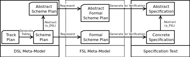
Figure 10. The OnTrack workflow.

1. Using a meta model for the formal specification language: The first option is to have a meta model describing the formal specification language. A Represent transformation translates a Scheme Plan into an equivalent Formal Scheme Plan over the meta model of the formal specification language. Then various Generate for Verification model to text transformations turn a Formal Scheme Plan into a Formal Specification Text ready for verification.

2. Direct generation of a formal specification: The second approach is to directly generate a formal specification. Thus only the Generate for Verification model to text transformations need to be implemented.

In both cases, the Generate for Verification transformations can enrich the models appropriately for verification, e.g. by including the DSL lemmas discussed earlier.

This horizontal workflow provides a transformation yielding a formal specification that faithfully represents a scheme plan. Here, we highlight the second approach that has been taken for the generation of Casl. The top level of the workflow shows the ability of OnTrack to include abstractions. We are interested in abstractions to ease verification. As abstractions do not play a role in our presentation in this paper, we refer the reader to [23] for the details.

OnTrack implements this overall workflow in a typical EMF/GMF/Epsilon architecture [9, 43, 27]. As a basis for our tool, we have taken the UML diagram in Figure 1 as our meta-model. Implementing a GMF front-end for this meta model involves selecting the concepts of the meta model that should become graphical constructs within the editor and assigning graphical images to them. Figure 11 shows the OnTrack editor which consists of a drawing canvas and a palette. Graphical elements from the palette can be positioned onto the drawing canvas. For example, a linear unit is now a drawable element.

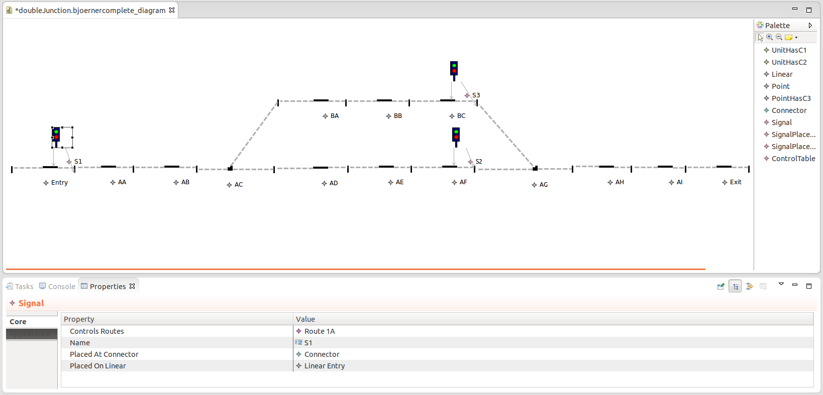
Figure 11. A screenshot of OnTrack modelling a station.

6.2.2. Generation of Formal CASL Specifications

Here we describe the direct implementation of the Generate for Verification transformations for Casl. The Generate for Verification transformation translates meta model instances of Bjørner’s DSL into formal specification text. This transformation is implemented using the Epsilon Generation Language (EGL) [27]. EGL allows template files to be written describing the text to be generated. These templates provide two main features for outputting text, namely the ability to output static text and to output dynamic text. Static text is considered text that is always generated independent of the model. Whilst Dynamic text is text that is text dependent on the given model. For this reason, Dynamic text is sometimes referred to as configuration data. By default, any text written in an EGL template is considered to be static text. For example we know that the specification of datatypes for our DSL and similarly our extension of this with dynamical aspects is the same for all models. Hence this is rather straightforwardly encoded as static text to be output, see Figure 12.

    spec Pair [sort S] [sort T] =
        sort Pair[S,T]
        ops first: Pair[S,T] -> S;
            second: Pair[S,T] -> T;
    ...
    spec StaticSignature =
         sorts Net, Station, Unit, Connector ...
         sorts Linear, Switch < Unit ...
         preds  __hasLine__: Net * Line;
    ...

Figure 12. Example of static text generation for our DSL.

Within the same EGL template, we can then specify the output for a concrete scheme plan. For example, consider the free type of units. Such a free type is built from the concrete elements of linear units and switch points contained within the graphical model. Hence we can specify the template in Figure 13 for the dynamic generation of the free type Unit. The result of applying this EGL fragment, to the concrete scheme plan in Figure 4 is the following Casl specification fragment:

free type Unit ::= lA1 | P1 | PLAT1 | PLAT2 | P2 | LA2.

1.  [% var rail : RailDiagram  := RailDiagram.allInstances().at(0); %]
2.  ...
3.  [%if(rail.hasUnits.size > 0){%]
4.      free type Unit ::=
5.      [%  var i := 0;
6.          while (i < rail.hasUnits.size()-1){ %]
7.          [%  var unit : Unit := rail.hasUnits.at(i);
8.             i := i+1; %]
9.             [%=unit.id%] | [%}%]
10.     [% var unit : Unit := rail.hasUnits.at(i); %]
11.     [%=unit.id%] [%}%]

Figure 13. Dynamic text generation for elements of Unit free type.

Considering Figure 13, the first construct of EGL that we notice is [% and %]. Any text specified between such a set of brackets is interpreted as code. For example, the line var rail : RailDiagram := ... is a line of EGL code for declaring the variable rail and assigning to it the current scheme plan instance within the graphical editor. This variable, can then be used throughout the EGL template to refer to the current model instance. Next, we see an EGL if statement (line 3). This statement checks the number of elements in the hasUnits relation of the current rail diagram. If there are linear units or points that have been drawn in the diagram, the code inside the if statement is executed. The first line within the if statement is static text to be generated. That is, as long as the if statement is entered, the text “free type Unit ::=” will be output. Lines 6 through to 9 perform a loop through the units of the concrete scheme plan instance. For each unit up until the last but one we can see, that in line 9, the dynamic text generation “[%=unit.id%]” is executed. Here, the dynamic text generation also contains the “=” symbol. This indicates that the text following is a piece of code that returns a value. For example, “unit.id” is a field containing the name that has been given to the current unit element. This name will then be output by the generation process. This dynamic text generation is immediately followed by the static text generation “|”. This produces the “|” symbol between elements of the free type. Finally, after the while statement there is another block of code (lines 10 and 11) that outputs the last unit identifier in the collection. For this unit, there is no static generation of the “|” symbol which matches the expected output for a Casl free type.

In a similar manner to the presented free type generation, it is possible to explore all the elements of the diagram generating the concrete scheme plan specification in Casl. After generation of the scheme plan, the safety property to be proven over the scheme plan can also be generated. As this property is the same for all scheme plans, this is simply generated as static text. The result is a full Casl specification ready for verification of the current editor model instance.

Overall, this generation means that OnTrack achieves the aim of automating the production of formal specifications from a graphical model. OnTrack is a toolset that is usable by engineers from the railway domain and allows them to produce formal Casl specifications ready for verification. This meets the third objective of our methodology as it makes formal specification available to domain engineers in an accessible format. The overall result from our methodology is a graphical tooling environment that incorporates a “push button” verification process for the railway signalling domain.

6.3. Contribution: Verification Results

Each of the track plans in Figure 14 (TP-A to TP-D) have been modelled using our DSL.

((a)) A pass through station (TP-A).

((b)) A double junction (TP-B).

((c)) A terminal station (TP-C).

((d)) A modified track plan from a London Underground station (TP-D).

Figure 14. Verified track plans.

We have then included a then then%implies block for the proof of safety. This block is also generated automatically by the OnTrack tool, as all information required for this block is available from the graphical model. The block is structured in two parts, the first contains lemmas to be proven, then the second our overall proof goal. The aim of the lemmas from the first block is to encode a case distinction used in the proof of safety. That is, they help the automated prover in proving our final goal. For verification using our DSL, these lemmas are in the form of our final proof goal instantiated for each route of the scheme plan under consideration. That is, for a route R, we have:

$\forall$ t $:$ Time; rg $:$ Region; ma $:$ MA
	$\bullet$	assigned(	ma, t) $\wedge$	rg eps ma $\wedge$	rg eps regions(R) $\Rightarrow$ $\neg$	R isOpenAt t

Once the above implied axioms have been proven, they can be used to help deduce our overall proof goal:

then	%implies
	$\forall$ t $:$ Time; r $:$ Route; rg $:$ Region; ma $:$ MA
		$\bullet$	assigned(	ma, t) $\wedge$	rg eps ma $\wedge$	rg eps regions(r) $\Rightarrow$ $\neg$	r isOpenAt t

The verification times presented in Figure 15 show that verification is possible over our enriched DSL. The average memory column shows the average memory used across all route lemma proofs and the safety proof. The proofs have been performed on a quad core $3$GHz machine with $8$GB of RAM running Ubuntu 12.04.

Track Plan	Routes Lemma Proofs (s)	Safety Proof (s)	Avg. Memory (MB)
TP-A	54.54	10.04	176.88
TP-B	23.88	6.57	90.36
TP-C	194.41	22.34	188.07
TP-D	236.10	20.46	489.64

Figure 15. Verification times for the given track plans.

All proofs are completed relatively quickly, with the longest proof time being for track plan TP-D. Interestingly, this is due to the number of units contained within this track plan. Also, it is interesting to note that the track plans that look more complicated and contain more possible routes, i.e. TP-B and TP-C are relatively quick to verify. This is because these track plans get split into many smaller regions compared with the fewer larger regions of track plan TP-D. Each of these small regions is represented by a list containing fewer elements within our modelling. Hence, the automated theorem prover does not need to search to such a depth to find a proof. This point is also illustrated by the increased average memory usage for TP-D. This shows that the DSL lemmas we have introduced give a measurable effect for verification. We note that these times outperform the typical times for model checking on such stations as, e.g., as presented in [33].

7. Related Work

At this point, we reflect on other DSL based approaches for railway verification, commenting on how they differ to our presented methodology.

The Railway Control Systems Domain language (RCSD) is a DSL for railway control systems developed by Kirsten Mewes [30]. RCSD is motivated by model-driven engineering approaches to system design. The language uses common domain notation for its concrete syntax and incorporates knowledge from domain engineers about the domain into its static and dynamic semantics. Mewes also considers the topic of testing models created in DSL. Here, domain specific constraints are included into the models ensuring that validation checks for correct functionality can be tested at the model level, before any software is been developed. Mewes’ work focuses on the design of RCSD. In contrast, we leave the design of the DSL to the domain engineer and focus on capturing domain knowledge that can be exploited for automatic verification.

Work by Haxthausen and Peleska [10] has also explored the development of a domain specific framework for automated construction and verification of railway control systems. Their framework consists of a three tiered approach: the top layer is a DSL for use by domain engineers to specify railway control systems; the second tier is model generation: A generator automatically produces the model of a control program based on the specification given by the design engineer. Bounded model checking can then be performed to establish various safety properties over such programs; the third tier allows actual code to be automatically generated and verified to ensure certain properties are maintained throughout process. Differing to our work, this framework is specifically developed for the railway domain and tied to a specific DSL. In this paper, we provide a generic and systematic methodology, where the railway domain serves for illustration.

Finally, the SafeCap toolset [11] provides a tooling platform that supports reasoning about railway capacity whilst ensuring system safety. It is based upon the SafeCap DSL, which captures track topology, route and path definitions and signalling rules. Overall, the toolset allows signalling engineers to design stations and junctions, to check their safety and to evaluate the potential improvements in capacity. Again, the SafeCap approach is bound to a specific DSL, where the design of the DSL is tailored to the underlying verification technology (Event B). This differs from our aim to decouple the DSL from the formal specification language, in turn allowing tooling environments to be very openly extendable.

8. Reflection on Industrial Collaboration

Since 2007, the Railway Verification Group at Swansea University Computer Science has been working in collaboration with Invensys Rail. The group is supported by eight academics. It adopts formal techniques to railway systems. This setup has led to a rich process of information exchange, by mutual visits and internships, as well as regular meetings. Out of this collaboration, there have been several successful research projects covering research into verification of interlocking programs [25, 24, 21, 15, 28, 18], the verification of scheme plan designs [32, 33, 23, 20], and capacity analysis [13]. These projects have involved many specification formalisms including propositional logic, CSP, Timed CSP, CSP$||$B, Scade, Casl and Agda. Here, it appears that operational based models such as the one we have provided in Casl are easier for railway engineers to follow and understand.

The methodology outlined in this paper has also been successfully applied to the Invensys Rail Data Model [12], see [16] for full details. In this context, the DSL definition is provided by Invensys Rail in the form of UML class diagrams with accompanying narrative. This DSL definition has been completely designed by Invensys Rail without our support. Hence, developing the informal DSL that is used as a starting point for our methodology is clearly a task that can be undertaken purely within industry. With regards to the formalisation of the DSL in Casl, this step was performed in a cyclic manner. Namely, the computer scientists would suggest a formalisation at a meeting with Invensys Rail, and then feedback would be provided on the formalisation. This process was repeated until both groups were happy with the resulting formalisation. Verification support (in terms of supporting lemmas) was then developed purely by the computer scientists at Swansea. As this step does not alter the DSL, the engineers were happy with the approach.

Finally, the graphical front end to the OnTrack tool provides a view to scheme plans that is of the same nature as representations used within Invensys Rail. The railway engineers have seen the verification process we propose and are confident that they could follow it thanks to the automated nature of the process. They have expressed an interest in the extension of OnTrack to allow for importing and exporting of models using an industrial format such as the XLDL (XML Layout Description Language) format used by Invensys Rail. This would allow the toolset to be more easily integrated within current development processes at Invensys Rail. We note that even though Invensys Rail believe technologies such as the OnTrack toolset will improve their development processes, due to concerns around the integrity of automated verification tools, quality assurance of a scheme plan design will, in the near future, still rely upon traditional testing and inspection. Here, tool qualification is the issue: our tools are not yet “proven-in-use”, i.e., there is no experience from previous industrial safety-critical projects suggesting that our tools are “correct”; alternatively, our tools are not yet certified by a designated authority.

Finally, it remains future work to perform a systematic evaluation into how usable the presented verification is for railway engineers. To do this, one could carry out a pilot project. This would involve thorough time measurement and documentation for all activities that our approach incurs including installing, using, and integrating OnTrack into the development process. Reflecting upon these results would allow us to check if our approach is indeed feasible. On the management level, such a pilot project would then have to be evaluated as to whether it is an improvement with respect to current practice. It should be both more effective, in that it allows one to achieve better results than current practice, and more efficient, i.e., it should offer a better cost/result ratio.

9. Summary & Conclusion

In this paper, we have introduced a novel design methodology for encapsulating formal methods within DSLs. We have supported our hypothesis that DSLs can aid with verification by showing it to be valid for the railway domain.

Our methodology begins with industrial documents describing domain elements in the form of UML class diagrams with narratives. This informal DSL is formalised in the algebraic specification language Casl, where we support this step with automated translations of the UML class diagram, thus ensuring “faithful modelling” of the domain. Next, systematic exploitation of domain knowledge allows us to prove domain specific lemmas. Thanks to these domain specific lemmas, properties on the formal specifications can automatically be proven for a class of systems, thus addressing issues surrounding “scalability”. Finally, a graphical editor for the DSL is developed. This editor allows engineers from the domain to follow a seamless verification process: (1) they can formulate models in the DSL; (2) these models can be automatically transformed into formal specifications; and (3) they can automatically verify these models thanks to the domain specific lemmas. Overall, this addresses the issues of “accessibility”of formal methods.

The verification of railway control software has been identified as a grand challenge of computer science [14]. The defining element of a grand challenge is that progress towards the challenge results in progress in computer science in general. Therefore, motivated by the railway domain, our methodology can be seen as a step forward for industrial applications of formal methods.

Along with presenting this methodology, we have also successfully illustrated the use of algebraic specification for modelling railway systems and the use of automated theorem proving for railway verification. Bringing these points together results in a strong case for using DSLs in the setting of specification and verification.

In the future, we would like to explore visual feedback of failed proof attempts. Currently, feedback to the user is provided in the form of a named route which is unsafe (obtained from the name of the failed proof). Such visualisations have been considered by Marchi et al. [7], and it would be interesting to extend OnTrack with such visualisations. We would also like to illustrate the applicability of our methodology to further domains, such as to the design of medical devices as considered by Oladimeji et al. [39].

Acknowledgements:

The authors would like to thank Simon Chadwick and Dominic Taylor from Invensys Rail UK for their contributions and encouraging feedback. We would like to thank our colleagues from the Swansea railway verification group and the Swansea Processes and Data research group for their input and feedback towards this work. Similarly, we greatly appreciate the input of Alexander Knapp and Till Mossakowski towards our work on the UML institution and comorphism to ModalCasl. We also thank Helen Treharne, Steve Schneider and Matthew Trumble from Surrey University for their collaboration in developing the OnTrack tool. Our final thanks goes to Erwin R. Catesbeiana (Jr) for signalling us in the correct direction.

Appendix A Domain Specific Lemma Proof

Proof: Following from the axioms presented in Section 4.3. we have:

:

$\Leftarrow$: Let us assume (**). The proof is given by induction on time $t$.

In the base case (t=$0$), (*) is true. This is the case as only the empty movement authority is assigned at time $0$ (given by axiom %(no_ma_0)%). Let $m1$, $m2$ be two movement authorities such that $share(m1,m2)$ holds. We consider two cases:

(1) if $m1=m2$ then the implication holds trivially;

(2) if $m1\not=m2$ then only one of these movement authorities can be the empty movement authority. Let, without loss of generality, $m1\not=[]$. Then $assigned(m1,0)$ is false (by axiom %(no_ma_0)%), hence the implication holds.

For the step case we have to show that:

$\forall$ t $:$ Time $\bullet$
	($\forall$ m1, m2 $:$ MA $\bullet$ share(m1, m2)
		$\Rightarrow$ m1 $=$ m2 $\vee$ $\neg$ (assigned(m1, $t$) $\wedge$ assigned(m2, $t$))) %(ih)%
	$\Rightarrow$
	($\forall$ m1, m2 $:$ MA $\bullet$ share(m1, m2)
		$\Rightarrow$ m1 $=$ m2 $\vee$ $\neg$ (assigned(m1, $suc(t)$) $\wedge$ assigned(m2, $suc(t)$)))

Let us assume (ih) for all movement authorities $m1,m2$. Let $m1^{\prime}$, $m2^{\prime}$ be two movement authorities such that $share(m1^{\prime},m^{\prime})$ holds. We consider two cases:

(1) if $m1^{\prime}=m2^{\prime}$ then the implication holds trivially;

(2) if $m1^{\prime}\not=m2^{\prime}$ then we need to show $\neg$ (assigned(m1’, t) $\wedge$ assigned(m2’, t)). By case distinction over the definition of the predicate assigned (axiom %(assigned_defn)%), we show that (assigned(m1’, t) $\wedge$ assigned(m2’, t)) is not possible and hence the implication holds.

• Case 1: (assigned(m1’, $suc(t)$) $\wedge$ assigned(m2’, $suc(t)$)) $\Rightarrow$ (assigned(m1’, t) $\wedge$ assigned(m2’, t) does not hold as it contradicts the assumed induction hypothesis (ih).

• Case 2: (assigned(m1’, $suc(t)$) $\wedge$ assigned(m2’, $suc(t)$)) $\Rightarrow$ canExtend(m1’, t) $\wedge$ canExtend(m2’, t), does not hold as it contradicts with axiom%(one_ma_changes)% stating that only one movement authority extends per time step.

• Case 3: (assigned(m1’, $suc(t)$) $\wedge$ assigned(m2’, $suc(t)$)) $\Rightarrow$ assigned(m1’, t) $\wedge$ canExtend(m2’, t). Given that share(m1’, m2’) holds, by the definition of the predicate $share$ (axiom %(share_defn)%) we know that there exists a region $rg$ such that $rg\in$ m1’ and $rg\in$ m2’. Let us consider, what it means for canExtend(m2’, t) to hold, i.e. instantiating axiom %(extend_defn)% with $m2^{\prime}$ gives:

  canExtend(	m2’, t) $\Leftrightarrow$
  		$\exists$ ma $:$ MA; r $:$ Route $\bullet$
  				assigned(	ma, t) $\wedge$ ext(	ma, r, m2’) $\wedge$	r isOpenAt t $\wedge$
  			(	$\neg$	ma $=$	$[$$]$ $\Rightarrow$ $\neg$ assigned(	ma, suc(t)))

  Hence, we have two cases to consider for the shared region $rg$:

  (1) if $rg\in$ ma, then by (**), all routes $r^{\prime}$ such that $rg\in regions(r^{\prime})$ are not open. Hence given axiom %(ext_defn)% which tells us that ext acts like list concatenation we know that $\neg\;r\;isOpenAt\;t$. Thus we have a contradiction that $canExtend(m2^{\prime},t)$ must hold, but also $\neg\;r\;isOpenAt\;t$ must hold;

  (2) if $rg\not\in$ ma then we know due to axiom %(ext_defn)% that $share(m1^{\prime},ma)$ holds. We also know, by the definition of canExtend (axiom %(extends_defn)%) that $assigned(ma,t)$ holds and similarly by our case assumption that $assigned(m1^{\prime},t)$ holds. Now if $m1^{\prime}\not=ma$ then we gain a contradiction to our induction hypothesis (ih). Whereas, if $m1^{\prime}=ma$, then by the definition of $canExtend$ (axiom %(extends_defn)%) we know that $\neg assigned(ma,suc(t))$ and hence that $\neg assigned(m1^{\prime},suc(t))$. This again contradicts our case assumption that $assigned(m1^{\prime},t)$ holds.

• Case 4: (assigned(m1’, $suc(t)$) $\wedge$ assigned(m2’, $suc(t)$)) $\Rightarrow$ canExtend(m1’, t) $\wedge$ assigned(m2’, t): Analogous to Case 3.

• Case 5-9: The remaining cases involve the reduction of one movement authority that is already assigned. Hence, each case follows from the definition of the canReduce predicate %(reduces_defn)% and our induction hypothesis (ih).

:

$\Rightarrow$: Let us assume (*). The proof is by contradiction.

We assume (**) does not hold, that is, we know there exists a route $r$ such that:

$\exists$ t $:$ Time; r $:$ Route; rg $:$ Region; ma $:$ MA
	$\bullet$ assigned(ma, t) $\wedge$ rg eps ma $\wedge$ rg eps regions(r)
		$\Rightarrow$ r isOpenAt t

Given this, this route can be used for an extension to another movement authority even though it is assigned. Assume at some time $t^{\prime}$, such that $suc(t^{\prime})=t$ there exist movement authorities $ma1,ma2$ such that $ext(ma1,rma2)$ and $rg\;eps\;ma2$. Then the predicate $canExtend$ (axiom %(extends_defn)%) holds for $ma2$ at time $t$. Thus, by the definition of assigned (axiom %(assigned_defn)%) $ma2$ can become assigned at time $suc(t^{\prime})$, i.e. time $t$. Now we have the situation that $assigned(ma,t)$ and $assigned(ma2,t)$ hold, but so does $share(ma,ma2)$ (axiom %(share_defn)%) over the region $rg$. Hence we have a contradiction to (**).

Appendix B Specification Structure

Throughout the paper, we have introduced various levels of specification that are structured as follows:

spec DSLForVerification $=$
	Datatypes
then
	DSL
then
	DSLExtension
then	%implies
	DSLemmas
then
	ConcreteSchemePlan
then	%implies
	Safety
end

Here we can see, that our specifications begin with the Datatypes (Datatypes) and DSL (DSL) gained from our translation of the UML class diagram. We then extend these specifications with DSLExtension for modelling the narrative aspects of the original informal DSL. Concretely this includes our modelling of movement authorities. Next, we can see that the property supporting lemmas (DSLemmas) are added to aid with verification. These are added as implied axioms over the extended DSL. This illustrates that these lemmas are independent of any scheme plan formulated in the DSL. Next, we see the specification ConcreteSchemePlan that encodes a particular track plan and its associated movement authorities and control tables. Finally, we can see the proof goals for proving safety are added (Safety). These are again added as implied axioms, and are then proven relative to the given concrete scheme plan.

References

- [1] J. E. Barnes. Experiences in the industrial use of formal methods. In A. Romanovsky, C. Jones, J. Bendiposto, and M. Leuschel, editors, AVoCS’11. Electronic Communications of EASST, 2011.
- [2] D. Bjørner. Dynamics of Railway Nets: On an Interface between Automatic Control and Software Engineering. CTS2003: 10th IFAC Symposium on Control in Transportation Systems, 2003.
- [3] D. Bjørner. Domain Engineering Technology Management, Research and Engineering. Japan Advanced Institute of Science and Technology, 2009.
- [4] J. Boulanger and M. Gallardo. Validation and verification of METEOR safety software. In j. Allen, R. J. Hill, C. A. Brebbia, G. Sciutto, and S. Sone, editors, Computers in Railways VII, volume 7, pages 189–200. WIT Press, 2000.
- [5] J. P. Bowen and M. G. Hinchey. Ten commandments of formal methods …ten years later. IEEE Computer, 39(1):40–48, 2006.
- [6] M. V. Cengarle, A. Knapp, A. Tarlecki, and M. Wirsing. A Heterogeneous Approach to UML Semantics. In P. Degano, R. De Nicola, and J. Meseguer, editors, Concurrency, Graphs and Models, LNCS 5065, pages 383–402. Springer, 2008.
- [7] O. M. dos Santos, J. Woodcock, and R. F. Paige. Using model transformation to generate graphical counter-examples for the formal analysis of xUML models. In ICECCS, pages 117–126. IEEE Computer Society, 2011.
- [8] ERTMS User Group. ERTMS/ETCS system requirements specification, 2002.
- [9] R. C. Gronback. Eclipse Modeling Project: A Domain-Specific Language (DSL) Toolkit. Addison-Wesley Professional, 2009.
- [10] A. Haxthausen and J. Peleska. A domain-oriented, model-based approach for construction and verification of railway control systems. In Formal Methods and Hybrid Real-Time Systems, volume 4700 of LNCS, pages 320–348. Springer, 2007.
- [11] A. Iliasov and A. Romanovsky. The SafeCap toolset for improving railway capacity while ensuring its safety. Technical report, Newcastle University, 2012.
- [12] Invensys Rail. Invensys Rail Data Model – Version 1A, 2010.
- [13] Y. Isobe, F. Moller, H. N. Nguyen, and M. Roggenbach. Safety and Line Capacity in Railways - An Approach in Timed CSP. In J. Derrick, S. Gnesi, D. Latella, and H. Treharne, editors, IFM, volume 7321 of Lecture Notes in Computer Science, pages 54–68. Springer, 2012.
- [14] R. Jacquart, editor. IFIP 18th World Computer Congress, Topical Sessions. 2004.
- [15] P. James. SAT-based Model Checking and its applications to Train Control Software. Master’s thesis, Swansea University, 2010.
- [16] P. James. Designing Domain Specific Languages for Verification and Applications to the Railway Domain. PhD thesis, Swansea University, 2014. Available at: http://cs.swan.ac.uk/~cspj/Papers/thesis.pdf.
- [17] P. James, A. Beckmann, and M. Roggenbach. Using domain specific languages to support verification in the railway domain. In Hardware and Software: Verification and Testing, volume 7857 of LNCS. Springer, 2013.
- [18] P. James, K. Kanso, A. Lawrence, F. Moller, M. Roggenbach, M. Seisenberger, and A. Setzer. Verification of solid state interlocking programs. In FM-RAIL-BOK 2013, To Appear, 2013.
- [19] P. James, A. Knapp, T. Mossakowski, and M. Roggenbach. Designing Domain Specific Languages – A Craftsman’s Approach for the Railway Domain using CASL. In WADT 2012, volume 7841 of LNCS. Springer, 2013.
- [20] P. James, F. Moller, H. N. Nguyen, M. Roggenbach, S. Schneider, H. Treharne, M. Trumble, and D. Williams. Verification of Scheme Plans using CSPB. In FM-RAIL-BOK 2013, To Appear, 2013.
- [21] P. James and M. Roggenbach. Automatically Verifying Railway Interlockings using SAT-based Model Checking. In J. Bendispoto, M. Leuschel, and M. Roggenbach, editors, AVoCS’10. Electronic Communications of EASST, 2010.
- [22] P. James and M. Roggenbach. Designing domain specific languages for verification: First steps. In G. S. Peter Hofner, Annabelle McIver, editor, ATE-2011, volume 760 of CEUR Workshop Proceedings. CEUR-WS.org, 2011.
- [23] P. James, M. Trumble, H. Treharne, M. Roggenbach, and S. Schneider. OnTrack: An open tooling environment for railway verification. In Proceedings of NFM’13, 2013.
- [24] K. Kanso. Formal Verification of Ladder Logic. Master’s thesis, Swansea University, 2008.
- [25] K. Kanso, F. Moller, and A. Setzer. Verification of safety properties in railway interlocking systems defined with ladder logic. In M. Calder and A. Miller, editors, AVoCS’08. Glasgow University, 2008.
- [26] D. Kerr and T. Rowbotham. Introduction To Railway Signalling. Institution of Railway Signal Engineers, 2001.
- [27] D. Kolovos, L. Rose, R. Paige, and F. Polack. The Epsilon Book, 2013.
- [28] A. Lawrence. Verification of Railway Interlockings in Scade. Master’s thesis, Swansea University, 2011.
- [29] M. Mernik, J. Heering, and A. M. Sloane. When and how to develop domain-specific languages. ACM Computing Survey, 37(4):316–344, 2005.
- [30] K. Mewes. Domain-specific Modelling of Railway Control Systems with Integrated Verification and Validation. PhD thesis, University of Bremen, 2010.
- [31] A. Mirabadi and B. Yazdi. Automatic generation and verification of railway interlocking control tables using FSM and NuSMV. Signal, 3, 2009.
- [32] F. Moller, H. N. Nguyen, M. Roggenbach, S. Schneider, and H. Treharne. CSPB Modelling for Railway Verification: The Double Junction Case Study. In AVoCS’12. Electronic Communications of EASST, 2012.
- [33] F. Moller, H. N. Nguyen, M. Roggenbach, S. Schneider, and H. Treharne. Defining and Model Checking Abstractions of Complex Railway Models using CSPB. In A. Biere, A. Nahir, and T. Vos, editors, Hardware and Software: Verification and Testing, volume 7857 of LNCS. Springer, 2013.
- [34] T. Mossakowski. Relating Casl with other specification languages: The institution level. Theoretical Computer Science, 286(2):367–475, 2002.
- [35] T. Mossakowski. ModalCASL — Specification with Multi-Modal Logics. Language Summary, 2004.
- [36] T. Mossakowski, C. Maeder, and K. Lüttich. The Heterogeneous Tool Set, Hets. In TACAS, volume 4424 of LNCS, pages 519–522. Springer, 2007.
- [37] P. D. Mosses, editor. CASL Reference Manual, volume 2960. Springer, 2004.
- [38] Object Managment Group. Unified Modeling Language (UML), v2.4.1, 2011.
- [39] P. C. Patrick Oladimeji, Paolo Masci and H. Thimbleby. Pvsio-web: a tool for rapid prototyping device user interfaces in PVS. In Proceedings of the 5th International Workshop on Formal Methods for Interactive Systems (FMIS 2013). Electronic Communications of EASST, 2013.
- [40] J. Peleska, D. Große, A. E. Haxthausen, and R. Drechsler. Automated verification for train control systems. In E. Schnieder and G. Tarnai, editors, Proceedings of Formal Methods for Automation and Safety in Railway and Automotive Systems. Technical University of Braunschweig, 2004.
- [41] S. Schneider and H. Treharne. CSP theorems for communicating B machines. Formal Aspects of Computing, 17(4):390–422, 2005.
- [42] S. Schulz. E-a brainiac theorem prover. AI Communications, 15(2):111–126, 2002.
- [43] D. Steinberg, F. Budinsky, E. Merks, and M. Paternostro. EMF: Eclipse Modeling Framework. Pearson Education, 2008.
- [44] C. Weidenbach, U. Brahm, T. Hillenbrand, E. Keen, C. Theobalt, and D. Topic. SPASS version 2.0. In A. Voronkov, editor, Automated Deduction – CADE-18, volume 2392 of LNCS, pages 275–279. Springer, 2002.
- [45] K. Winter. Model checking railway interlocking systems. Australian Computer Science Communications, 24(1):303–310, 2002.
- [46] K. Winter and N. J. Robinson. Modelling large railway interlockings and model checking small ones. In M. J. Oudshoorn, editor, ACSC ’03: Proceedings of the 26th Australasian computer science conference. Australian Computer Society, 2003.