Charmonium Spectral Functions and Transport Properties of Quark-Gluon Plasma

Abstract

We study vacuum masses of charmonia and the charm-quark diffusion coefficient in the quark-gluon plasma based on the spectral representation for meson correlators. To calculate the correlators, we solve the quark gap equation and the inhomogeneous Bethe-Salpeter equation in the rainbow-ladder approximation. It is found that the ground-state masses of charmonia in the pseudoscalar, scalar, and vector channels can be well described. For $1.5\,T_{c}<T<3.0\,T_{c}$, the value of the diffusion coefficient $D$ is comparable with that obtained by lattice QCD and experiments: $3.4<2\pi TD<5.9$. Relating the diffusion coefficient with the ratio of shear viscosity to entropy density $\eta/s$ of the quark-gluon plasma, we obtain values in the range $0.09<\eta/s<0.16$.

The charmonium system is a bound state of a charmed quark–anti-quark pair. The first charmonium state $J/\psi$ was found simultaneously at BNL [1] and at SLAC [2] in 1974. Charmonium spectroscopy plays the same role [3, 4] for understanding the strong interaction, described by quantum chromodynamics (QCD), as does the spectroscopy of positronium or of the hydrogen atom for the electromagnetic interaction, described by quantum electrodynamics (QED).

Charm quarks are also produced in hard parton interactions in the early stage of heavy-ion collisions, e.g. at the Relativistic Heavy Ion Collider (RHIC) and the Large Hadron Collider (LHC). During the further evolution of the fireball, these quarks interact with the quark-gluon plasma (QGP) created in such collisions. The ensuing loss of energy of a charm quark is different from the one experienced by light quarks [5, 6]. A comparison between the energy loss for light quarks with that for heavy ones can provide insight into properties of the QGP.

Even in a hot and dense medium, charm quarks can form bound states with other light or heavy quarks. The formation and dissociation of these states depends on the properties of the surrounding medium. For instance, it was proposed [7] that, due to color screening, the formation of $J/\psi$ is suppressed in the QGP, which can serve as a signal of the deconfinement phase transition. More recent calculations within lattice QCD [8, 9, 10, 11], however, show that the $J/\psi$ may actually survive up to temperatures exceeding the critical temperature $T_{c}$ of the deconfinement and chiral phase transition. Therefore, it is an interesting and meaningful task to understand charmonium properties in vacuum and medium systematically.

A first-principle method to study charmonium properties is lattice QCD. Within this approach, the charmonium spectrum, including ground, excited, and exotic states, has been computed at zero temperature, $T=0$ [12, 13, 14], finding rather good agreement with experimental data. Transport properties, e.g., the charm quark diffusion coefficient, which are closely related to charmonium spectral functions, are also calculable within lattice QCD [15, 16]. The charm quark diffusion coefficient has also been studied within a $T$-matrix approach [17] and a relativistically covariant approach based on QCD sum rules [18].

Assuming that the interaction between charm quarks can be described by a potential, one can adopt nonrelativistic potential models to study charmonium properties [19]. The parameters of the potential can be adjusted to the vacuum charmonium spectrum. In order to study charmonia at nonzero temperatures, one can generalize the vacuum potential to a temperature-dependent one based on models [20] or lattice-QCD results [21].

Dyson-Schwinger equations (DSEs) [22, 23] which include both dynamical chiral symmetry breaking and confinement serve as a nonperturbative continuum approach for studying QCD. At $T=0$, DSEs have been used to study properties of bound states, e.g., the light and heavy hadron spectrum [24, 25], pion properties [26, 27], as well as hadron form factors [28, 29]. At $T\neq 0$, the chiral and deconfinement transitions and the excitations in the QGP have been studied through solving the quark gap equation [30, 31]. Recently, a novel spectral representation has been developed to study in-medium hadron properties and the electrical conductivity of the QGP [32]. These results are consistent with experiment and lattice QCD, which establishes the DSE approach as a powerful and reliable tool to study the properties of hadrons and strong-interaction matter.

In this work, we employ DSEs to study charmonium spectral functions and transport properties of the QGP. First, we calculate the charmonium spectrum at $T=0$ in order to fix the charm quark current mass. Then, we study the charm quark number susceptibility (QNS) and diffusion coefficient at $T>T_{c}$. At last, we use a formula obtained by perturbation theory to translate the diffusion coefficient to the ratio of shear viscosity to entropy density, i.e., $\eta/s$, of the QGP.

In the imaginary-time formalism of thermal field theory [33], the Matsubara correlation function of a local meson operator $J_{H}(\tau,\vec{x}\,)$ is defined as

$$\Pi_{H}(\tau,\vec{x}\,)=\langle J_{H}(\tau,\vec{x}\,)J_{H}^{\dagger}(0,\vec{0}\,)\rangle_{\beta}\;,$$ (1)

where $\beta=1/T$, $\tau$ is the imaginary time with $0<\tau<\beta$, and $\langle\ldots\rangle_{\beta}$ denotes the thermal average. The operator $J_{H}$ has the following form

$$J_{H}(\tau,\vec{x}\,)=\bar{q}(\tau,\vec{x}\,)\gamma_{H}q(\tau,\vec{x}\,)\;,$$ (2)

with $\gamma_{H}=\mathbf{1},\gamma_{5},\gamma_{\mu},\gamma_{5}\gamma_{\mu}$ for scalar, pseudo-scalar, vector, and axial-vector channels, respectively.

In terms of Green functions the meson correlation functions are defined as

$$\parbox{204.85983pt}{\includegraphics[width=433.62pt]{cor}}\;,$$ (3)

where gray circular blobs denote dressed propagators $S$ and vertices $\Gamma_{H}$, $G^{(4)}$ denotes the full quark–anti-quark four-point Green function, $G_{0}^{(4)}$ denotes the two disconnected dressed quark propagators in the dashed box, and black dots denote bare propagators or vertices.

The dressed quark propagator $S$ is a solution of the quark gap equation which reads

$$\parbox{184.9429pt}{\includegraphics[width=433.62pt]{gap}}\;.$$ (4)

The dressed quark propagator depends on the dressed gluon propagator $D_{\mu\nu}^{ab}$ and the dressed quark-gluon vertex $\Gamma_{\mu}^{a}\,$. The dressed quark propagator $S(\tilde{\omega}_{n},\vec{p}\,)$ can be generally decomposed as

$$S=1/[i\vec{\gamma}\cdot\vec{p}\,A(\tilde{\omega}_{n}^{2},\vec{p}\,^{2})+i\gamma_{4}\tilde{\omega}_{n}\,C(\tilde{\omega}_{n}^{2},\vec{p}\,^{2})+B(\tilde{\omega}_{n}^{2},\vec{p}\,^{2})]\;,$$

where $\tilde{\omega}_{n}=(2n+1)\pi T,\,n\in Z$, are the fermionic Matsubara frequencies, and $A,B$, and $C$ are scalar functions. The mass scale of quarks can be defined as

$$M_{0}=\frac{B(\tilde{\omega}_{0}^{2},\vec{0}\,)}{C(\tilde{\omega}_{0}^{2},\vec{0}\,)}\;.$$ (5)

The dressed vertex $\Gamma_{H}$ satisfies the inhomogeneous Bethe-Salpeter equation (BSE),

$$\parbox{176.40707pt}{\includegraphics[width=433.62pt]{bse}}\;,$$ (6)

where $K^{(2)}$ denotes the two-particle irreducible kernel. The above equation needs the dressed quark propagator as input. Its solution can be decomposed according to the $J^{P}$ quantum number of the corresponding meson channel $H$.

Inserting the solutions of Eqs. (4) and (6) into Eq. (3), we obtain the imaginary-time charmonium correlation functions. However, for solving Eqs. (4) and (6), we have to specify $D_{\mu\nu}^{ab}$, $\Gamma_{\mu}^{a}$, and $K^{(2)}$. To this end, we use the abelian rainbow-ladder (RL) approximation. The rainbow part of this approximation consists of (color indices are suppressed)

$$g^{2}D_{\mu\nu}(k_{\Omega})\Gamma_{\nu}(\tilde{\omega}_{n},\vec{p}\,;\tilde{\omega}_{l},\vec{q}\,)=D^{\rm eff}_{\mu\nu}(k_{\Omega})\gamma_{\nu}\;,$$ (7)

with the effective gluon propagator written as

$$D^{\rm eff}_{\mu\nu}(k_{\Omega})=P^{T}_{\mu\nu}\mathcal{D}(k_{\Omega}^{2})+P^{L}_{\mu\nu}\mathcal{D}(k_{\Omega}^{2}+m_{g}^{2})\;,$$ (8)

where $k_{\Omega}=(\tilde{\omega}_{n}-\tilde{\omega}_{l},\vec{p}\,-\vec{q}\,)$, $P^{T,L}_{\mu\nu}$ are transverse and longitudinal projection tensors, respectively, $\mathcal{D}$ is the gluon dress function which describes the effective interaction, and $m_{g}$ is the gluon Debye mass. The ladder part of the RL approximation is given by

$$K^{(2)}(\tilde{\omega}_{n},\vec{p}\,;\tilde{\omega}_{l},\vec{q}\,)=D^{\rm eff}_{\mu\nu}(k_{\Omega})[(i\gamma_{\mu})\otimes(i\gamma_{\nu})]\;,$$ (9)

which expresses the two-particle irreducible kernel in terms of one-gluon exchange. Note that the RL approximation is the leading term in a symmetry-preserving approximation scheme. The solutions of Eqs. (4) and (6) satisfy Ward-Takahashi identities [34, 35, 36].

Now the quark gap equation and the inhomogeneous BSE, i.e., Eqs. (4) and (6), can be self-consistently solved once the gluon dress function $\mathcal{D}$ is given. Here, the modern one-loop renormalization-group-improved interaction model [37, 38] is adopted. This model has two parameters: a width $\xi$ and a strength $d$. With the product $\xi d$ fixed and $\xi\in[0.4,0.6]$ GeV, one can obtain a uniformly good description of pseudoscalar and vector mesons in vacuum with masses $\lesssim 1$ GeV. We use $\xi=0.5$ GeV. At $T>T_{c}$, we introduce a Debye mass $m_{g}$ in the longitudinal part of the gluon propagator and a logarithmic screening for the nonperturbative interaction [31, 32] in order that physical quantities, e.g., the thermal quark masses for massless quarks and the electrical conductivity of the QGP, are consistent with lattice QCD [39, 40].

All information which we are interested in is embedded in the spectral function of the charmonium correlation function. In energy-momentum space, the spectral function is defined as the imaginary part of the retarded correlation function,

$$\rho_{H}(\omega,\vec{p}\,) = 2\,{\rm Im}\,\Pi_{H}^{R}(\omega,\vec{p}\,)\;,$$ (10)

$$= 2\,{\rm Im}\Pi_{H}(i\omega_{n},\vec{p}\,)|_{i\omega_{n}\to\omega+i\epsilon}\;,$$

where $\omega_{n}=2n\pi T,\,n\in Z$, are the bosonic Matsubara frequencies. Then, the spectral representation at zero momentum ($\vec{p}\,=\vec{0}\,$) reads

$$\Pi_{H}(\omega_{n}^{2})=\int_{0}^{\infty}\frac{d\omega^{2}}{2\pi}\frac{\rho_{H}(\omega)}{\omega^{2}+\omega_{n}^{2}}-({\rm subtraction})\;,$$ (11)

where the dependence of $\Pi_{H}$ on $\omega_{n}$ is quadratic, since it is an even function of $\omega_{n}$ at $\vec{p}\,=\vec{0}\,$. An appropriate subtraction is required because the spectral integral does not converge for meson correlation functions, i.e., $\rho_{H}(\omega\to\infty)\propto\omega^{2}$. This divergence manifests itself in a corresponding divergence of the loop integral in Eq. (3).

In order to solve the divergence problem, one of us (S.Q.) has suggested to introduce a discrete transform for $\Pi_{H}$ [32],

$$\hat{\Pi}_{H}(\omega_{n_{1}}^{2},\omega_{n_{2}}^{2},\omega_{n_{3}}^{2})=\sum_{i=1}^{3}\Pi_{H}(\omega_{n_{i}}^{2})\prod_{j\neq i}^{3}\frac{1}{\omega_{n_{i}}^{2}-\omega_{n_{j}}^{2}}\;,$$ (12)

where $\omega_{n_{1}}\neq\omega_{n_{2}}\neq\omega_{n_{3}}$. Then, we can obtain the well-defined spectral representation

$$\begin{split}\hat{\Pi}_{H}(\omega_{n_{1}}^{2},\omega_{n_{2}}^{2},\omega_{n_{3}}^{2})=\int_{0}^{\infty}\frac{d\omega^{2}}{2\pi}\,\rho_{H}(\omega)\prod_{i=1}^{3}\frac{1}{\omega^{2}+\omega_{n_{i}}^{2}}\;.\end{split}$$ (13)

By introducing a one-variable correlator as $\tilde{\Pi}_{H}(\omega_{n}^{2})=\hat{\Pi}_{H}(\omega_{n}^{2},\omega_{n+1}^{2},\omega_{n+2}^{2})$, we can reduce Eq. (13) to a one-dimensional equation for numerical convenience.

At $T=0$, the Matsubara frequencies become continuous and the system has an $O(4)$ symmetry. Then, the spectral representation (13) can be written in an $O(4)$ covariant form. The charmonium spectrum in vacuum can be extracted from the spectral function $\rho_{H}(\omega)$.

At $T\neq 0$, especially, $T>T_{c}$, a charmonium state, e.g., $J/\psi$, can survive up to a certain temperature above which it dissolves. With increasing $T$, the corresponding peak in the spectral function becomes broader and decreases in height, and finally disappears altogether. Qualitatively, we may identify the charmonium dissociation temperature as the temperature where the charmonium peak in the spectral function becomes indistinguishable from the background.

Of great interest are transport properties of charm quarks because they reflect the dynamics of the QGP. Several transport coefficients can be extracted from the electromagnetic (i.e., vector) current correlation function $\Pi_{V}^{\mu\nu}$. First, the QNS is defined as

$$\chi_{00}=\frac{\partial n(\mu,T)}{\partial\mu}\bigg{|}_{\mu=0}=\Pi_{V}^{44}(0)\;,$$ (14)

where $n(\mu,T)$ is the quark number density. The second equality is derived from the vector Ward identity – a result of vector-current conservation. According to Eq. (3), $\Pi_{V}^{44}$ only depends on the dressed vector vertex and quark propagator, i.e., $\Gamma_{V}^{\mu}$ and $S$. In the non-interacting quasi-particle approximation, $\Gamma_{V}^{\mu}=\gamma^{\mu}$ and $S=1/[i\vec{\gamma}\cdot\vec{p}\,+i\gamma_{4}\tilde{\omega}_{n}+M_{0}]$. Then, $\chi_{00}$ is given by

$$\chi_{00}=-4N_{c}\int\frac{d^{3}\vec{k}}{(2\pi)^{3}}\frac{\partial n_{f}(E_{\vec{k}})}{\partial E_{\vec{k}}}\;,$$ (15)

where $E_{\vec{k}}=\sqrt{M_{0}^{2}+\vec{k}\,^{2}}$ is the quasi-particle energy, and $n_{f}$ is the Fermi distribution function.

Without the quasi-particle approximation, we have to evaluate the QNS numerically. To this end, we turn to the spectral representation Eq. (13). From Eqs. (11) and (14), the zeroth component of the vector spectral function can be written as

$$\rho_{V}^{00}(\omega)=2\pi\chi_{00}\omega\delta(\omega)\;.$$ (16)

Inserting this into Eq. (13), we have

$$\chi_{00}=\hat{\Pi}_{V}^{44}(\omega_{n_{1}}^{2}=0,\omega_{n_{2}}^{2},\omega_{n_{3}}^{2})\,\omega_{n_{2}}^{2}\,\omega_{n_{3}}^{2}\;,\$$ (17)

which is well-defined and equivalent for any $\omega_{n_{2}}\neq\omega_{n_{3}}\neq 0$. In comparison to Eq. (14), the above expression is much easier to calculate numerically.

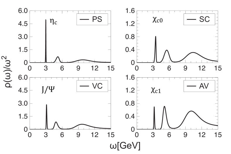
Figure 1: Charmonium spectral functions at zero temperature.

Table 1: The Euclidean constituent mass of the charm quark and charmonium masses at zero temperature ($m^{\zeta}_{c}=0.79$GeV, $\zeta=19$GeV, and dimensional quantities are given in GeV).

	$m^{E}_{c}$	$\eta_{c}$	$J/\psi$	$\chi_{c0}$	$\chi_{c1}$
this work	1.396	2.980	3.113	3.476	3.227
PDG	1.275	2.980	3.097	3.415	3.510

From the Kubo formula, the heavy quark diffusion coefficient can be expressed as

$$D=\frac{1}{6\chi_{00}}\lim_{\omega\to 0}\sum_{i=1}^{3}\frac{\rho_{V}^{ii}(\omega)}{\omega}\;,$$ (18)

where $\rho_{V}^{ii}$ are the spatial components of the vector spectral function (in what follows, the summation is suppressed unless stated). In Ref. [41], Moore and Teaney perturbatively calculated the ratio of $D$ to the transport coefficient $\eta/(\epsilon+p)$, where $\epsilon$ is the energy density and $p$ is the pressure. It is found that for a QGP with two light flavors, the ratio is around $6$ and has a weak dependence on the coupling strength. Using the thermodynamic identity $\epsilon+p=sT$ (at zero chemical potential), we can translate $D$ to $\eta/s$ as

$$\frac{\eta}{s}\approx\frac{1}{6}TD\;.$$ (19)

In order to extract the spectral function from $\hat{\Pi}_{H}$ which is given by the solution of the DSE, we adopt the maximum entropy method (MEM) [42, 43, 44]. At $T=0$, we follow lattice-QCD studies [45] and choose the MEM default model as $m_{\rm fr}\omega^{2}$, where the coefficient $m_{\rm fr}$ is calculated in the non-interacting limit [46, 47]. The results are shown in Fig. 1. In each channel, the first peak is sharp. This means that the ground-state signal is strong. The corresponding masses are listed in Table 1, where the pseudoscalar channel $\eta_{c}$ is fitted by adjusting the current charm quark mass $m_{c}^{\zeta}$, and the Euclidean constituent mass of the charm quark $m^{E}_{c}:=\{\sqrt{p^{2}}\,|\,p^{2}>0,{p^{2}}=B^{2}(p^{2})/A^{2}(p^{2})\}$ (because of the $O(4)$ symmetry at $T=0$, $A=C$ are functions of four-momentum squared $p^{2}$). It is found that, with the exception of the axial-vector channel, all masses agree well with their experimental values. The $\chi_{c1}$ mass (and similarly the $a_{1}$ mass) comes out noticeably smaller than the experimental value, because the RL approximation misses the anomalous chromomagnetic effect in the quark-gluon vertex [48]. Going beyond the RL approximation [24, 29], one can remedy this drawback. Nevertheless, it is safe to use the RL approximation for the vector channel.

Next, we study the QNS of charmed quarks in the QGP. The result calculated by Eq. (17) (denoted by $\chi_{00}$) is shown in the upper panel of Fig. 2. For comparison, we also present the result obtained by the quasi-particle formula (15) (denoted by $\chi_{00}^{\rm QP}$). As illustrated in the lower panel of Fig. 2, the ratio $\chi_{00}^{\rm QP}/\chi_{00}$ decreases with increasing temperature, which means that the quasi-particle picture works well at high temperature, but fails in the neighborhood of $T_{c}$.

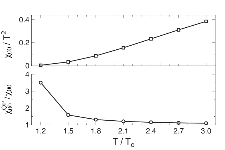
Figure 2: The heavy quark number susceptibility (the upper panel) and the ratio to that obtained in the quasi-particle picture (the lower panel) as a function of temperature.

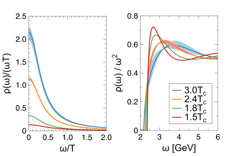
Figure 3: The vector spectral function at different temperatures, where the shaded regions around the curves (produced by changing the MEM default model) provide an estimate for the systematic error.

At $T>T_{c}$, it is assumed that the vector spectral function has two parts, i.e., a low-energy transport peak and a continuous part above $2M_{0}$. Then, we prepare the default model as

$$\rho_{V}^{ii}(\omega) = \frac{6\chi_{00}T}{M_{0}}\frac{\omega\eta_{D}}{\omega^{2}+\eta_{D}^{2}}+\frac{3}{2\pi}\Theta\left(\omega^{2}-4M_{0}^{2}\right)$$ (20)

$$\times~{}\omega^{2}\tanh\left({\omega}/{4T}\right)\sqrt{1-{4M_{0}^{2}}/{\omega^{2}}}$$

$$\times~{}\left[1+{4M_{0}^{2}}/{\omega^{2}}\right]\;,$$

where $\eta_{D}=\frac{T}{M_{0}D}$ is the drag coefficient. Note that, as for $T=0$, there is no resonance peak specified in the continuous part.

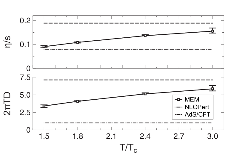
Figure 4: The ratio $\eta/s$ and the heavy quark diffusion coefficient as a function of temperature. The dashed line is obtained by an NLO perturbative calculation at $T=3T_{c}$, and the dot-dashed line is given by AdS/CFT. The error bars are obtained by altering the default model.

In order to completely determine the default model, we need prior information on $\eta_{D}$. In the neighborhood of $T_{c}$, i.e., $T\gtrsim T_{c}$, we assume the system to be a strongly coupled QGP, where the AdS/CFT correspondence gives $\eta_{D}=\frac{2\pi T^{2}}{M_{0}}$ [49]. At high temperature, e.g., $T\gtrsim 3T_{c}$, perturbative QCD at next-to-leading order (NLO) yields the thermal quark mass (for massless quarks) $m_{T}=\frac{g_{s}T}{\sqrt{6}}\left(1+1.867\frac{g_{s}}{4\pi}\right)$ [50] and the drag coefficient $\eta_{D}=\frac{8\pi T^{2}}{3M_{0}}\alpha_{s}^{2}\left(0.07428-\ln g_{s}+1.9026g_{s}\right)$ [51]. In our model, $m_{T}=0.8T$, then $g_{s}\approx 1.6$, $\alpha_{s}\approx 0.2$, and $\eta_{D}\approx\frac{0.9T^{2}}{M_{0}}$. To summarize, we make the Ansatz

$$\eta_{D}=\frac{\gamma T^{2}}{M_{0}}\;,$$ (21)

where $\gamma$ decreases with increasing $T$ for $T_{c}<T<3T_{c}$. Using a linear interpolation, we simply write

$$\gamma=\frac{1}{a+bT/T_{c}}\;,$$ (22)

where $a$ and $b$ can be determined by the two limiting cases.

The obtained vector spectral function is shown in Fig. 3, where the shaded regions around the curves correspond to the uncertainties by halving or doubling the height of the transport peak in the default model. Note that the uncertainties are relatively small. With increasing $T$, the resonance peak becomes broader and decreases in height, which indicates the dissociation of $J/\psi$. We estimate the dissociation temperature to be around $2T_{c}$. On the other hand, the transport peak in the low-energy region becomes higher with increasing $T$. Using Eq. (18) and inserting the result for the QNS, we extract the $T$-dependence of the heavy quark diffusion coefficient. Furthermore, we can estimate $\eta/s$ according to Eq. (19). The results are shown in Fig. 4. It is found that, for $1.5\,T_{c}<T<3.0\,T_{c}$, $\eta/s$ increases with $T$ and lies within the bounds given by the AdS/CFT and NLO-perturbative calculations, respectively.

In conclusion, combining a newly proposed spectral representation of the vector current correlation function with the self-consistent solutions of the quark gap equation and the inhomogeneous Bethe-Salpeter equation, we calculated the charm quark diffusion coefficient $D$ of the QGP. Our result is consistent with that obtained by lattice QCD [16, 15] and that extracted by the PHENIX experiment [52]. With Eq. (19), we used $D$ to estimate $\eta/s$. We found that $\eta/s$ increases with increasing $T$. The values for $\eta/s$ remain above the AdS/CFT bound [49] and are close to that obtained from a functional renormalization group calculation [53] and other estimates (see Ref. [52] and references therein). In the future, we plan to extend the study to nonzero chemical potential.

References

References

- [1] E598 Collaboration, J. Aubert et al., Phys. Rev. Lett. 33, 1404 (1974).
- [2] SLAC-SP-017 Collaboration, J. Augustin et al., Phys. Rev. Lett. 33, 1406 (1974).
- [3] M. Voloshin, Prog. Part. Nucl. Phys. 61, 455 (2008).
- [4] U. Wiedner, Nucl. Phys. News 20, 19 (2010).
- [5] X.-N. Wang and M. Gyulassy, Phys. Rev. Lett. 68, 1480 (1992).
- [6] E. Braaten and M. H. Thoma, Phys. Rev. D44, 2625 (1991).
- [7] T. Matsui and H. Satz, Phys. Lett. B178, 416 (1986).
- [8] S. Datta, F. Karsch, P. Petreczky, and I. Wetzorke, Phys. Rev. D69, 094507 (2004).
- [9] M. Asakawa and T. Hatsuda, Phys. Rev. Lett. 92, 012001 (2004).
- [10] G. Aarts, C. Allton, M. B. Oktay, M. Peardon, and J.-I. Skullerud, Phys. Rev. D76, 094513 (2007).
- [11] WHOT-QCD Collaboration, H. Ohno et al., Phys. Rev. D84, 094504 (2011).
- [12] C. Davies et al., Phys. Rev. D52, 6519 (1995).
- [13] CP-PACS Collaboration, M. Okamoto et al., Phys. Rev. D65, 094508 (2002).
- [14] J. J. Dudek, R. G. Edwards, N. Mathur, and D. G. Richards, Phys. Rev. D77, 034501 (2008).
- [15] D. Banerjee, S. Datta, R. Gavai, and P. Majumdar, Phys. Rev. D85, 014510 (2012).
- [16] H. Ding et al., Phys. Rev. D86, 014509 (2012).
- [17] D. Cabrera and R. Rapp, Phys. Rev. D76, 114506 (2007).
- [18] P. Gubler, K. Morita, and M. Oka, Phys. Rev. Lett. 107, 092003 (2011).
- [19] E. Eichten, K. Gottfried, T. Kinoshita, K. Lane, and T.-M. Yan, Phys. Rev. D21, 203 (1980).
- [20] A. Mocsy, Eur. Phys. J. C61, 705 (2009).
- [21] O. Kaczmarek and F. Zantow, Phys. Rev. D71, 114510 (2005).
- [22] C. D. Roberts and A. G. Williams, Prog. Part. Nucl. Phys. 33, 477 (1994).
- [23] C. Roberts, Prog. Part. Nucl. Phys. 61, 50 (2008).
- [24] L. Chang and C. D. Roberts, Phys. Rev. C85, 052201 (2012).
- [25] M. Blank and A. Krassnigg, Phys. Rev. D84, 096014 (2011).
- [26] L. Chang, I. Cloet, C. Roberts, S. Schmidt, and P. Tandy, arXiv:1307.0026 [nucl-th] (2013).
- [27] L. Chang et al., Phys. Rev. Lett. 110, 132001 (2013).
- [28] P. Maris and C. D. Roberts, Int. J. Mod. Phys. E12, 297 (2003).
- [29] L. Chang, C. D. Roberts, and P. C. Tandy, Chin. J. Phys. 49, 955 (2011).
- [30] S.-x. Qin, L. Chang, Y.-x. Liu, and C. D. Roberts, Phys. Rev. D84, 014017 (2011).
- [31] S.-x. Qin and D. H. Rischke, Phys. Rev. D88, 056007 (2013).
- [32] S.-x. Qin, arXiv:1307.4587 [nucl-th] (2013).
- [33] M. Le Bellac, Thermal Field Theory (Cambridge University Press, 2000).
- [34] J. S. Ball and T.-W. Chiu, Phys. Rev. D22, 2542 (1980).
- [35] S.-X. Qin, L. Chang, Y.-X. Liu, C. D. Roberts, and S. M. Schmidt, Phys. Lett. B722, 384 (2013).
- [36] S.-X. Qin, C. D. Roberts, and S. M. Schmidt, arXiv:1402.1176 [nucl-th] (2014).
- [37] S.-x. Qin, L. Chang, Y.-x. Liu, C. D. Roberts, and D. J. Wilson, Phys. Rev. C84, 042202 (2011).
- [38] S.-x. Qin, L. Chang, Y.-x. Liu, C. D. Roberts, and D. J. Wilson, Phys. Rev. C85, 035202 (2012).
- [39] F. Karsch and M. Kitazawa, Phys. Rev. D80, 056001 (2009).
- [40] A. Amato et al., arXiv:1307.6763 [hep-lat] (2013).
- [41] G. D. Moore and D. Teaney, Phys. Rev. C71, 064904 (2005).
- [42] R. K. Bryan, Eur. Biophys. J 18, 165 (1990).
- [43] D. Nickel, Annals Phys. 322, 1949 (2007).
- [44] J. A. Mueller, C. S. Fischer, and D. Nickel, Eur. Phys. J. C70, 1037 (2010).
- [45] M. Asakawa, T. Hatsuda, and Y. Nakahara, Prog. Part. Nucl. Phys. 46, 459 (2001).
- [46] F. Karsch, E. Laermann, P. Petreczky, and S. Stickan, Phys. Rev. D68, 014504 (2003).
- [47] G. Aarts and J. M. Martinez Resco, Nucl. Phys. B726, 93 (2005).
- [48] L. Chang, Y.-X. Liu, and C. D. Roberts, Phys. Rev. Lett. 106, 072001 (2011).
- [49] P. Kovtun, D. T. Son, and A. O. Starinets, JHEP 0310, 064 (2003).
- [50] M. Carrington, A. Gynther, and D. Pickering, Phys. Rev. D78, 045018 (2008).
- [51] S. Caron-Huot and G. D. Moore, Phys. Rev. Lett. 100, 052301 (2008).
- [52] PHENIX Collaboration, A. Adare et al., Phys. Rev. C84, 044905 (2011).
- [53] M. Haas, L. Fister, and J. M. Pawlowski, arXiv:1308.4960 [hep-ph] (2013).