Measurement-based tailoring of Anderson localization of partially coherent light

Abstract

We put forward an experimental configuration to observe transverse Anderson localization of partially coherent light beams with a tunable degree of first-order coherence. The scheme makes use of entangled photons propagating in disordered waveguide arrays, and is based on the unique relationship between the degree of entanglement of a pair of photons and the coherence properties of the individual photons constituting the pair. The scheme can be readily implemented with current waveguide-on-a-chip technology, and surprisingly, the tunability of the coherence properties of the individual photons is done at the measurement stage, without resorting to changes of the light source itself.

I Introduction

More than 50 years ago, P. W. Anderson described in a seminal paper Anderson1958Absence how diffusion in the process of electron transport in a disordered (random) semiconductor lattice can be arrested, leading to the localization of the wavefunction in a small region of space, the so-called Anderson localization. This unique phenomenon has been observed in a myriad of physical systems Anderson2009PhysToday , including electron gas Cutler1969Observation , matter waves (atoms) Chabe2008Experimental ; Billy2008Direct ; Roati2008Anderson , and acoustic waves Hu2008Localization . The observation of transverse localization of light in a photonic system was predicted by De Raedt et al. Raedt1989Transverse , considering the similarities existing between the Schrödinger equation and Maxwell equations. This led to the observation of Anderson localization in photonic systems Wiersma1997Localization ; Schwartz2007Transport ; Schreiber2011Decoherence ; Crespi2013Anderson ; Lahini2008Anderson in various scenarios.

The underlying physical principles that lead to Anderson localization are also responsible for changes on the spreading of the wavefunction in a quantum random walk, characterized by a quadratic dependence of the size (variance) of the wavefunction with propagation distance when no disorder is present Aharonov1993Quantum ; Svozilik2012Implementation . The consequences of introducing static disorder in a quantum random walk (leading to Anderson localization) have been studied, for example, for one-dimensional Yin2008Quantum ; PerinaJr2009b ; PerinaJr2009c and two-dimensional Inui2004Localization systems. In a sense, generalizations of quantum protocols such as the Shor’s factorization algorithm Shor1994Algorithms and the Groover’s searching algorithm Grover1996Afast can also be analyzed in similar terms, since they can be viewed as quantum random walks.

In most cases, the input state in a quantum random walk is considered to be fully coherent. Since Anderson localization is a consequence of interference effects, one can dare thinking that an initial coherent state is thus necessary to observe Anderson localization. However, Čapeta et al. Capeta2011Anderson have shown that even a partially coherent input light beam can lead to Anderson localization in a disordered waveguide array (WGA). Partially coherent beams can be described as a superposition of orthogonal coherent modes, where the modal coefficients are random variables that are uncorrelated with one another mandel_book ; segev2001 . Therefore, according to Capeta2011Anderson , since spreading of each mode, being a coherent mode, can be arrested in a random medium with static disorder, the whole partially coherent beam should also suffer localization in a similar way to a fully coherent beam.

Here we propose an experimental scheme which could lead to the observation of Anderson localization of partially coherent beams with a tunable degree of first-order coherence. The approach is based on two basic ingredients. On the one hand, a single-photon in a pure quantum state (von Neumann entropy $E=0$) is arguably the most simple example of a photonic state which shows first-order coherence glauber1966 . Mixed single-photon quantum states do not show first-order coherence. On the other hand, the degree of entanglement of a pure two-photon state (photons A and B) is directly related to the purity of the quantum state of photon A (B), which results from tracing out all degrees of freedom corresponding to photon B (A). The von Neumann entropy of the quantum state that describes photon A (B) could be used as a measure of the degree of entanglement of the paired photons.

Consequently, the manipulation of the degree of entanglement of the two-photon state can effectively tailor the first-order coherence of the signal (idler) photon victor2009 , generating a one-photon quantum state which is mixed, and thus partially coherent. Anderson localization (co-localization) of entangled photon fields in disordered waveguides has been presented in Lahani2010Quantum ; Abouraddy2012Anderson ; DiGiuseppe2013Einstein . However, in that case the goal was to look for Anderson localization of the two photons that form the entangled pair, while here entanglement is a tool to tailor the degree of coherence of one of the subsystems (photon A or photon B) which form the entangled pair.

The paper is organized as follows. In Section II the experimental scheme and the main theoretical tools used in the analysis are presented and discussed. Main results are presented in Section III. The single-photon coherence measures used throughout the text are defined in the Appendix.

II The proposed experimental scheme

In general, the quantum description of a pure entangled two-photon state (photons A and B) is written

$$|\Psi\rangle=\int dp\int dq\,\Psi(p,q)\hat{a}_{A}^{\dagger}(p)\hat{a}_{B}^{\dagger}(q)|0\rangle$$ (1)

where $p$ and $q$ represent the transverse wavevectors of photons $A$ and $B$, respectively, $\hat{a}_{A}^{\dagger}(p)$ and $\hat{a}_{A}^{\dagger}(q)$ are creation operators of photons in modes $A$ and $B$, and $\Psi(p,q)$ is the mode function that describes the properties of the biphoton progress2011 . For monochromatic fields, the positive-frequency electric-field operators are expressed as

$$\hat{E}_{A}^{(+)}(x)\sim\int dp\,\hat{a}_{A}(p)\exp\left(ipx\right),$$ (2)

$$\hat{E}_{B}^{(+)}(y)\sim\int dq\,\hat{a}_{B}(q)\exp\left(iqy\right).$$ (3)

We note that temporal dependence of the electric-field operators has been omitted for the sake of simplicity. Defining $\Psi(x,y)=\int dp\,\int dq\,\Psi(p,q)\exp(-ipx-iqy)$, the normalized pure entangled two-photon state given by Eq. (1) can be written as

$$|\Psi\rangle=\int dx\int dy\,\Psi\left(x,y\right)|x\rangle_{A}|y\rangle_{B},$$ (4)

where we have defined $|x\rangle_{A}\equiv\hat{E}_{A}^{(-)}\left(x\right)|0\rangle_{A}$ and $|y\rangle_{B}\equiv\hat{E}_{B}^{(-)}\left(y\right)|0\rangle_{B}$. Notice that the two-photon amplitude $\Psi(x,y)$ corresponds to the second-order correlation function $\Psi(x,y)={}_{A}\langle 0|{}_{B}\langle 0|\hat{E}_{B}^{(+)}(y)\hat{E}_{A}^{(+)}(x)\rangle$.

The two-photon amplitude $\Psi$ can be described by a Schmidt decomposition of the form

$$\Psi(x,y)=\sum_{j=1}^{N}\sqrt{\lambda_{j}}f_{j}\left(x\right)g_{j}\left(y\right);$$ (5)

$\lambda_{j}$ are the Schmidt eigenvalues and $\{f_{j}\}$ and $\{g_{j}\}$ are the Schmidt modes corresponding to photons A and B. For the sake of simplicity, the two-photon amplitude $\Psi(x,y)$ is approximated by the Gaussian function

$$\Psi(x,y)\sim\exp\left[-\alpha\left(x+y\right)^{2}-\beta\left(x-y\right)^{2}\right].$$ (6)

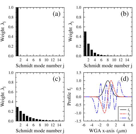
Figure 1: (Color online) Schmidt mode decomposition. Here we show the first $15$ Schmidt modes of the Schmidt decomposition for three cases: a) a separable state with $\gamma_{0}=0.5$, (b) an entangled state with $\gamma_{0}=1.5$, and (c) an entangled state with $\gamma_{0}=3$. The shape of some selected Schmidt modes (see the legend) are plotted in (d) for $\gamma_{0}=1.5$. In all cases $\sigma_{0}$ = 1 $\mu m$.

In this case, the Schmidt modes correspond to Hermite functions of order $j$ chan_eberly ; PerinaJr2008 . Some representative cases are shown in Fig.1(d).

The parameters characterizing the spatial correlations between photons $A$ and $B$, $\alpha$ and $\beta$, can be expressed using more suitable parameters that describe characteristics of photon A: its rms beam width ($\sigma_{0}$) and the beam width-spatial bandwidth product ($\gamma_{0}$), here denoted as incoherence,

$$\alpha = \frac{1}{4\sigma_{0}^{2}}\left(2\gamma_{0}^{2}\pm\gamma_{0}\sqrt{4\gamma_{0}^{2}-1}\right),$$ (7)

$$\beta = \frac{1}{4\sigma_{0}^{2}}\left(2\gamma_{0}^{2}\mp\gamma_{0}\sqrt{4\gamma_{0}^{2}-1}\right).$$ (8)

The derivation of Eq. (7) and Eq. (8) is included in the Appendix. In general, $\gamma_{0}\geq 0.5$ and is related to the Schmidt number, $K=2\gamma_{0}$, which is a measure of the size of the mode distribution involved in Eq. (5), i.e., $K=(\sum_{j=1}^{N}\lambda_{j})^{2}/\sum_{j=1}^{N}\lambda_{j}^{2}$. For $\alpha=\beta$, there is not entanglement between photons A and B, the Schmidt decomposition contains a single mode [see Fig. 1(a)], and $\gamma_{0}$ attains its minimum value, i.e., $\gamma_{0}=0.5$. This case yields a pure and first-order coherent photon. In all other cases, the spectrum of the Schmidt decomposition contains several modes. Fig.1(b) shows the weights of the first $15$ Schmidt modes (eigenvalues $\lambda_{j}$) for $\gamma_{0}=1.5$ and Fig.1(c) shows them for $\gamma_{0}=3$.

The key point of our scheme is the presence of a detection scheme that projects the photon $B$ into a restricted set of modes before detection, or in particular the projection into a single Schmidt mode $g_{j}$. In this way, the number of modes that describe the quantum state of photon A after detection of photon $B$ would be correspondingly reduced. Importantly, the first-order coherence of photon $A$ depends on the number of modes onto which the photon $B$ is projected. The projection of photon $B$ into a specific single mode effectively renders photon $A$ into a first-order coherent photon. In contrast, detection of photon $B$ into an increasing number of modes results in a partially coherent signal photon with a decreasing degree of coherence. Therefore, this can thus be appropriately called tailoring of the first-order coherence by heralding detection.

By tailoring the first-order coherence of a single photon, we also tailor the characteristics of the Anderson localization. The projection and detection of photon $B$ into a finite number $M$ of modes is represented by the quantum operator $\hat{Y}_{B}=\sum_{j=1}^{M}|g_{j}\rangle_{B}\langle g_{j}|_{B}$ with $|g_{j}\rangle=\int dyg_{j}(y)|y\rangle_{B}$. After detection, the truncated quantum state of photon A reads as

$$\hat{\rho}_{A}={\rm Tr}_{B}\left[|\Psi\rangle\langle\Psi|\hat{Y}_{B}\right]=\sum_{j=1}^{min\left(N,M\right)}\lambda_{j}|f_{j}\rangle_{A}\langle f_{j}|_{A}$$ (9)

corresponding to an incoherent superposition of $min\left(N,M\right)$ modes with weights $\lambda_{j}$.

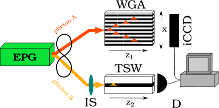
Figure 2: (Color online) Sketch of the experimental configuration proposed to observe Anderson localization of partially coherent photons in a disordered waveguide array (WGA). The three-slab waveguide (TSW) allows propagation of different numbers of guided modes depending on its core size. EPG: The Entangled-photons generator is the source of photon pairs; iCCD: intensified CCD; D: single-photon detector; IS: Imaging System.

A sketch of the experimental configuration considered is shown in Fig. 2. A pair of entangled photons (A and B) is generated. Photon A is injected into a one-dimensional waveguide array (WGA) with refractive index profile $n_{A}(x)$. The waveguide array contains $101$ layers of semiconductor material $Al_{x}Ga_{1-x}As$ with the index of reflection taken from Gehrsitz2000The . The whole structure is created by alternating two different layers: $Al_{0.3}Ga_{0.7}As$ and $Al_{0.8}Ga_{0.2}As$ of the same thickness 0.6 $\mu m$. The disorder is induced by randomizing the index of refraction of each layer, etc.: $n_{A}(x)=n^{0}_{A}(x)+\Delta n_{A}(x)$. The probability distribution of the random disturbances $\Delta n_{A}(x)$ is described by a Gaussian function characterized by its typical standard deviation $\delta$.

On the other hand, the photon B can propagate in different three-slab waveguides (TSWs) with refractive index profile $n_{B}(y)$, and different sizes of the core of the waveguide. The material of the core is $Al_{0.3}Ga_{0.7}As$ and two surrounding layers are made of $Al_{0.8}Ga_{0.2}As$. The layers surrounding the core are considered to be infinite in their thickness. The number of guided modes supported depends on the core size [see Fig.3(a)], so the three-slab waveguide effectively selects a certain amount of modes of photon B, effectively tailoring the first-order coherence of photon A. A three-slab waveguide has been chosen for simplicity, and because of its suitability for integration on a chip altogether with the WGA.

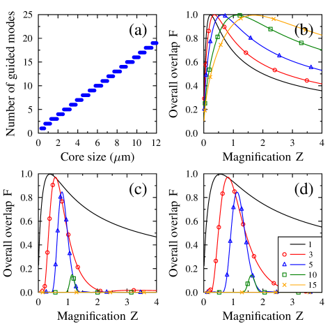
Figure 3: (Color online) (a) Number of guided modes supported by the three-slab waveguide (TSW) as a function of the core size of the waveguide. (b)-(d) show the overall spatial overlap factor between Schmidt modes $\{g_{j}\}$ and guided modes of the three-slab waveguide $\{v_{j}\}$, as given by the product $F=\prod_{j}|d_{jj}|$, as a function of the magnification factor Z of the imaging system. Three different cases, with different values of $\gamma_{0}$, are considered: (b) $\gamma_{0}=0.5$, (c) $\gamma_{0}=1.5$, and (d) $\gamma_{0}=3$. In all cases $\sigma_{0}$ = 1 $\mu m$. The five curves in each plot correspond to five different three-slab waveguides supporting various amounts of modes, as given by the legend in (d).

The evolution of the spatial shape of photons A and B, in the waveguide array and the three-slab waveguide, respectively, can be conveniently described by means of the guided modes supported by each waveguide, $\{u_{i}(x)\}$ for the WGA and $\{v_{j}(y)\}$ for the TSW Karbasi2013Modal . The guided modes are obtained as solutions of the Helmholtz equations

$$\Delta u_{i}(x)+\left[n_{A}^{2}(x)k_{0}^{2}-\kappa_{i}^{2}\right]u_{i}(x)=0,$$ (10)

$$\Delta v_{j}(y)+\left[n_{B}^{2}(y)k_{0}^{2}-\mu_{j}^{2}\right]v_{j}(y)=0,$$ (11)

where $\kappa_{i}$ and $\mu_{j}$ are the corresponding propagation constants. The index of refraction is considered to be homogeneous along the direction of propagation (along the $z$-axis in both waveguides). Equation (10) has been solved using the finite element method Jin2002Finite , whereas Eq. (11) has been solved by the semi-analytical method Snyder1983Optical . The polarization of photons A and B is transverse electric, i.e. parallel to the surface boundary between layers, and their wavelengths are $1550$ nm, far below the band gap of the material. Therefore, absorption can be omitted in our model. Moreover, the propagation distance $z_{1}$ of photon A has been restricted to 0.5 mm in order to prevent reaching the reflective boundaries of WGA.

The coupling of the input photons, characterized by the Schmidt modes $f_{n}$ and $g_{m}$, to the corresponding waveguides, characterized by modes $u_{i}$ and $v_{j}$, is expressed via the coupling coefficients

$$c_{ni}=\int dxf_{n}(x)u_{i}^{*}(x),$$ (12)

$$d_{mj}=\int dyg_{m}(y)v_{j}^{*}(y).$$ (13)

Using coefficients $c_{ni}$ and $d_{mj}$ the quantum state of two photons after their propagation at distances $z_{1}$ and $z_{2}$ in the two waveguides is

$$|\Psi\rangle=\sum_{n}\sqrt{\lambda_{n}}\sum_{ij}c_{ni}d_{n_{j}}$$

$$\times\exp\left(i\kappa_{i}z_{1}+i\mu_{j}z_{2}\right)|u_{i}\rangle_{A}|v_{j}\rangle_{B},$$ (14)

where $|u_{i}\rangle_{A}\equiv\int dxu_{i}(x)|x\rangle_{A}$ and $|v_{j}\rangle_{B}\equiv\int dyv_{j}(y)|y\rangle_{B}$. We can write $z_{1}=z_{2}=z$ without losing generality.

Detection of photon B after projection via a three-slab waveguide is represented by the operator $\hat{Y}_{B}=\sum_{i=j}^{n_{max}}|v_{j}\rangle_{B}\langle v_{j}|_{B}$, where $n_{max}$ refers to the limited amount of guided modes present in the specific three-slab waveguide considered. For fixed values of $\gamma_{0}$ and $\sigma_{0}$, the spatial profile of photon B is the same, but the spatial profiles of the guided modes $\{v_{j}\}$ differ in their sizes for waveguides with different core size. Modes of the Schmidt decomposition $\{g_{j}(y)\}$ and guide modes in the TSW $\{v_{j}(y)\}$ can be ordered by its mode order ($j=1,2,...$), with modes with the same order having similar spatial shapes. In order to maximize the spatial overlap between the Schmidt modes and the guided modes, we include an imaging system designed to maximize the overall spatial overlap factor $F=\prod_{j}|d_{jj}|$. Fig. 3(b),(c) and (d) show the overall spatial overlap factor as a function of the magnification factor (Z) of the imaging system for five different three-slab waveguides which support $1$, $3$, $5$, $10$, and $15$ guided modes, respectively. For instance, for $\sigma_{0}=1\mu$m and $\gamma_{0}=3$, the optimum magnification factors are $0.55$, $0.82$, $1.13$, $1.61$, and $2.03$.

In contrast, since we are interested in the Anderson localization of photon A after propagation in the disordered waveguide array, the spatial profile of photon A is detected by an intensified coupled-charge detector (iCCD), which allows us to detect electromagnetic signals at the single-photon level. Detection of a photon in each pixel of the iCCD is represented via the photon-number operator $\hat{n}_{A}\left(x\right)=\hat{E}^{(-)}_{A}\left(x\right)\hat{E}_{A}^{(+)}\left(x\right)$. After detection of photon $B$, the spatial shape of the photon A at distance $z$ in the WGA is described by the photon-number spatial distribution

$$p_{A}(x)=Tr_{A}\left[\hat{\rho}_{A}\hat{n}_{A}\left(x\right)\right]=\sum_{m,n}\sqrt{\lambda_{m}\lambda_{n}}I\left(m,n\right)$$

$$\times\sum_{i,j}c_{mi}c^{*}_{nj}\exp\left\{iz\left(\kappa_{i}-\kappa_{j}\right)\right\}u_{i}\left(x\right)u^{*}_{j}\left(x\right),$$ (15)

where $I\left(m,n\right)=\sum_{j}d_{mj}d^{*}_{nj}$. The width of photon $A$ can be characterized by its effective beam width

$$w_{eff}=\left\langle\frac{\left[\int dxp_{A}(x)\right]^{2}}{\int dxp_{A}^{2}(x)}\right\rangle,$$ (16)

where $\langle\rangle$ refers to averaging over an ensemble of random realizations of a disordered WGA.

In order to analyze the results presented in Sec. III, it is important to take into account that the beam size $\sigma_{0}$ and the incoherence $\gamma_{0}$ of photon $A$, defined in Eqs. (7) and (8), corresponds to values before projection and detection of photon $B$. Therefore, after filtering mediated by the spatial mode projection of photon B using the TSW, the first-order correlation function of photon A at the input of WGA is written

$$G_{A}^{(1)}(x,x^{\prime})=\sum_{m,n}\sqrt{\lambda_{n}\lambda_{m}}I\left(m,n\right)f_{n}\left(x\right)f^{*}_{m}\left(x^{\prime}\right).$$ (17)

One can obtain the values of $\sigma$ and $\gamma$ for photon $A$ via equations Eq. (22), Eq. (25) and Eq. (26) in the the Appendix.

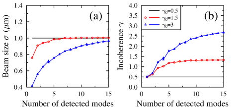
Figure 4: (Color online) (a) Beam size $\sigma$ and (b) incoherence $\gamma$ of photon A when photon B propagates in different TSWs, and afterwards is detected. Each TSW is designed to support a different number of guided modes, as indicated in the axis. We consider three different two-photon states (see legend in (b)), characterized by $\gamma_{0}=0.5$, 1, and 3. In all cases, $\sigma_{0}\,=\,1\,\mu m$.

If photon B propagates in a TSW that supports a single propagating mode, the size of photon A will corresponds to the size of that single mode, independently of the value of $\sigma_{0}$. When other modes are added via an increase of the guiding capability of TSW, the beam size $\sigma$ reaches its initial value $\sigma_{0}$, as it is shown in Fig. 4(a) for a photon with $\sigma_{0}=1\mu$m. A similar behavior of the value of $\gamma$ is also shown in Fig. 4(b), where a strong dependence on the effectiveness of the coupling to the TSW is observed. When coupling to a single mode, $\gamma=0.5$, independently of the value of $\gamma_{0}$. When the number of propagating modes in TSW is enlarged, the value of $\gamma$, even though it is smaller than $\gamma_{0}$, also converges to $\gamma_{0}$, since now propagation in the waveguide does not effectively filter the input state.

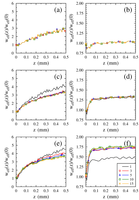
Figure 5: (Color online) Spreading of the size of photon A after propagation in the WGA, as given by the ratio $w_{eff}(z)/w_{eff}(0)$. Photons A and B are part of a two-photon state with three different values of the amount of entanglement, but with the same value of $\sigma_{0}$ = 1 $\mu m$. (a) and (b) correspond to a non-entangled two-photon state with $\gamma_{0}=0.5$ (K=1). (c) and (d) corresponds to an entangled state with $\gamma_{0}=1.5$ (K=3), while for (e) and (f) we have $\gamma_{0}=3$ (K=6). (a),(c), and (e) correspond to the propagation of photon A in a non-disordered WGA, while (b),(d), and (f) corresponds to the propagation of photon A in a disordered WGA with $\sigma=0.02$. We present averaged results obtained over 100 different realizations of WGA. The curves in all plots represent propagation of photon B in different TSW which support distinct amounts of guided modes, as shown in the legend in (f). This legend is valid for all plots.

III Results

For the sake of comparison, we first consider a separable two-photon state ($K=1$), so the Schmidt decomposition contains a single mode, as shown in Fig. 1(a). Photon A is in a first-order coherent state, and since there is no entanglement, there is also no dependence on the characteristics of the propagation of photon A on photon B being projected and detected. As expected, when no disorder is considered ($\delta=0$), photon A diffracts the least in comparison to other cases considered in Figs.5(c) and (e), which corresponds to entangled paired photons. When disorder is introduced ($\delta=0.02$), photon A turns out to be localized, with the size of the output probability distribution being almost equal to the input probability. Anderson localization is the result of the coupling of photon A to localized guided modes of the disordered WGA $\{u_{i}(x)\}$.

We now consider two examples with two-photon entangled states with $\gamma_{0}=1.5$ and 3. This corresponds to two-photon states with Schmidt number $K=3$ and 6, and entropy of entanglement $E=2$ and 3.021. The Schmidt decompositions are shown in Fig. 1(b) and (c). Unlike the coherent case ($\gamma_{0}$=0.5), the size of photon A depends on the amount of propagating modes of the TSW used. This phenomenon is more visible with the ordered WGA, as shown in Fig. 5(c) and (e). Note that each Hermite function $\{f_{i}\}$ for $i>1$ contains high spatial components that spread even faster than the narrow Gaussian profile given by $f_{1}$, but in the overall, they might have a smaller impact on the final size of photon A due to decreasing weights $\lambda_{j}$ for a given state.

For a disordered WGA with $\delta=0.02$ the effect of the partially coherent nature of photon A values on its propagation is more visible, as seen in Fig. 5(d) and (f). The lower the degree of coherence, the broader is the output effective width of the spatially localized photon A. Moreover, Hermite functions $\{f_{i}\}$ with increasing order localize with a higher ratio $w_{eff}(L)/w_{eff}(0)$ than the fundamental Hermite function $f_{1}$. Our calculations also predict a noticeable dependence of the amount of localization expected, shown in Fig. 5, on important experimental values such as the magnification factor of the imaging system or the effectiveness of the coupling to the TSW. Therefore, if one were to use a different optimization function $F$ for the imaging system, differences in Fig. 5(d) and 5(f) would be more visible.

IV Conclusion

We have presented an experimental scheme for the observation of transverse Anderson localization of partially coherent light with a tunable degree of coherence. The degree of coherence is tuned by injecting one photon of a fully coherent two-photon entangled state in a waveguide with a finite and controllable amount of propagating modes. The system can be integrated on a semiconductor chip, since both the disordered waveguide array (WGA) and the three-slab waveguide (TSW) considered were designed with this goal in mind. Therefore our proposal is experimentally feasible taking into an account current mature semiconductor technologies.

Appendix

IV.1 Quantifying the first-order coherence of the single photon

The two-photon states given by Eqs. (1) and (4) describes a generally entangled state. The density matrix that characterizes the quantum state of one of the photons that constitute the pair, for instance $\hat{\rho}_{A}$ for photon A, is obtained by tracing out the variables describing photon B, so

$$\hat{\rho}_{A}=\int dx\int dx^{\prime}\rho_{A}(x,x^{\prime})|x\rangle_{A}\langle x^{\prime}|_{A},$$ (18)

where

$$\rho_{A}(x,x^{\prime})=\int dy\Psi\left(x,y\right)\Psi^{*}\left(x^{\prime},y\right).$$ (19)

Notice that $\rho_{A}(x,x^{\prime})$ is the well-known first-order correlation function $G_{A}^{(1)}(x,x^{\prime})$ of photon A, defined as

$$G_{A}^{(1)}(x,x^{\prime})={\rm Tr}\left[\hat{\rho}_{A}\hat{E}_{A}^{(-)}\left(x\right)\hat{E}_{A}^{(+)}\left(x^{\prime}\right)\right],$$ (20)

where $\hat{E}_{A}^{(+)}$ and $\hat{E}_{A}^{(-)}$ are the positive- and negative-frequency electric-field operators mandel_book . The first-order correlation function for photon B is defined similarly.

Making use of Eqs. (6) and (19), we obtain

$$G_{A}^{(1)}(x,x^{\prime}) \sim \exp\left[-\left(\alpha+\beta\right)x^{2}-\left(\alpha+\beta\right)x^{\prime 2}\right.$$ (21)

$$\left.+\frac{\left(\alpha-\beta\right)^{2}}{2\left(\alpha+\beta\right)}\left(x+x^{\prime}\right)^{2}\right].$$

The Gaussian form of the two-photon amplitude, as defined in Eq. (6), allows us to quantify the width of photon A in the position space using $G_{A}^{(1)}(x,x^{\prime})$. The rms spatial width of photon A is

$$\sigma^{2}=\frac{\int dx\,x^{2}G_{A}^{(1)}(x,x)}{\int dx\,G_{A}^{(1)}(x,x)}=\frac{\alpha+\beta}{16\alpha\beta}.$$ (22)

The two-photon amplitude $\Psi(p,q)$ in the transverse wave-number domain is equal to

$$\Phi(q,k)\sim\exp\left[-\frac{\left(q+k\right)}{16\alpha}^{2}-\frac{\left(q-k\right)^{2}}{16\beta}\right].$$ (23)

Similarly to the case considered above, the first-order correlation function in the transverse wave-number domain reads

$$G_{A}^{(1)}(q,q^{\prime})={\rm Tr}\left[\hat{\rho}_{A}\,\hat{a}_{A}^{\dagger}(q)\hat{a}_{A}(q^{\prime})\right].$$ (24)

One can calculate the rms width of photon A in the transverse wave-number domain as

$$W^{2}=\frac{\int dq\,q^{2}G_{A}^{(1)}(q,q)}{\int dq\,G_{A}^{(1)}(q,q)}=\alpha+\beta.$$ (25)

Here we quantify the first-order coherence of photon A as the product of its spatial beam width ($\sigma$) by its width in the transverse wavevector domain ($W$)

$$\gamma=\sigma W=\frac{\alpha+\beta}{4\sqrt{\alpha\beta}},$$ (26)

this parameter $\gamma$ represents the amount of incoherence. For more details concerning quantification of coherence, see Perina1991 . Making use of Eqs. (22) and (26) one easily obtains Eqs. (7) and (8) in the main text. The minimum value of $\gamma$ is $\gamma=0.5$. It corresponds to a separable two-photon state with $\alpha=\beta$. In this case, photon A (and photon B) shows first-order coherence. For entangled states, photon A is described by an incoherent superposition of Hermite-Gauss modes, whose number increases with a corresponding increase of the degree of entanglement between photons A and B. Therefore, increasing values of $\gamma$ correspond to photons with a lower degree of coherence.

References

- (1) P. W. Anderson, Phys. Rev. 109, 1492 (1958).
- (2) A. Lagendijk, B. van Tiggelen, and D. S. Wiersma, Phys. Today 62, 24 (2009).
- (3) M. Cutler and N. F. Mott, Phys. Rev. 181, 1336 (1969).
- (4) J. Chabé, G. Lemarié, B. Grémaud, D. Delande, P. Szriftgiser, and J. C. Garreau, Phys. Rev. Lett. 101, 255702 (2008).
- (5) J. Billy, V. Josse, Z. Zuo, A. Bernard, B. Hambrecht, P. Lugan, D. Clément, L. Sanchez-Palencia, P. Bouyer, and A. Aspect, Nature 453, 891 (2008).
- (6) G. Roati, C. D`Errico, L. Fallani, M. Fattori, C. Fort, M. Zaccanti, G. Modugno, M. Modugno, and M. Inguscio, Nature 453, 895 (2008).
- (7) H. Hu, A. Strybulevych, J. H. Page, S. E. Skipetrov, and B. A. van Tiggelen, Nat. Phys. 4, 945 (2008).
- (8) H. De Raedt, A. Lagendijk, and P. de Vries, Phys. Rev. Lett. 62, 47 (1989).
- (9) D. S. Wiersma, P. Bartolini, A. Lagendijk, and R. Righini, Nature 390, 671 (1997).
- (10) T. Schwartz, G. Bartal, S. Fishman and M. Segev, Nature 446, 52 (2007).
- (11) A. Schreiber, K. N. Cassemiro, V. Potoček, A. Gábris, I. Jex, and Ch. Silberhorn, Phys. Rev. Lett. 106, 180403 (2011).
- (12) A. Crespi, R. Osellame, R. Ramponi, V. Giovannetti, R. Fazio, L. Sansoni, F. De Nicola, F. Sciarrino, and P. Mataloni, Nat. Photon. 7, 322 (2013).
- (13) Y. Lahini, A. Avidan, F. Pozzi, M. Sorel, R. Morandotti, D. N. Christodoulides, and Y. Silberberg, Phys. Rev. Lett. 100, 013906 (2008).
- (14) Y. Aharonov, L. Davidovich, and N. Zagury, Phys. Rev. A 48, 1687 (1993).
- (15) J. Svozilík, R. de J. León-Montiel, and J. P. Torres, Phys. Rev. A 86, 052327 (2012).
- (16) Y. Yin, D. E. Katsanos, and S. N. Evangelou, Phys. Rev. A 77, 022302 (2008).
- (17) J. Peřina Jr., M. Centini, C. Sibilia, and M. Bertolotti, J. Russ. Laser Res. 30, 508 (2009).
- (18) J. Peřina Jr., M. Centini, C. Sibilia, and M. Bertolotti, Phys. Rev. A 80, 033844 (2009).
- (19) N. Inui, Y. Konishi, and N. Konno, Phys. Rev. A 69, 052323 (2004).
- (20) P. W. Shor, in Proc. 35nd Annual Symposium on Foundations of Computer Science, Santa Fe, 1994, edited by S. Goldwasser (IEEE Computer Society Press, Washington, 1994), p. 124.
- (21) L. K. Grover, in Proc. 28th Annual ACM Symposium on Theory of Computing, Philadelphia, 1996, edited by G. L. Miller (ACM New York, 1996), p. 212.
- (22) D. Čapeta, J. Radić, A. Szameit, M. Segev, and H. Buljan, Phys. Rev. A 84, 011801 (2011).
- (23) L. Mandel and E. Wolf, Optical coherence and quantum optics, Cambridge University Press, New York, 1995.
- (24) D. N. Christodoulides, E. D. Eugenieva, T. H. Coskun, M. Segev, and M. Mitchell, Phys. Rev. E 63, 035601 (2001).
- (25) U. M. Titulaer and R. J. Glauber, Phys. Rev. 145, 1041 (1966).
- (26) V. Torres-Company, A. Valencia, and J. P. Torres, Opt. Lett. 34, 1177 (2009).
- (27) Y. Lahini, Y. Bromberg, D. N. Christodoulides, and Y. Silberberg, Phys. Rev. Lett. 105, 163905 (2010).
- (28) A. F. Abouraddy, G. Di Giuseppe, D. N. Christodoulides, and B. E. A. Saleh, Phys. Rev. A 86, 040302 (2012).
- (29) G. Di Giuseppe, L. Martin, A. Perez-Leija, R. Keil, F. Dreisow, S. Nolte, A. Szameit, A. F. Abouraddy, D. N. Christodoulides, and B. E. A. Saleh, Phys. Rev. Lett. 110, 150503 (2013).
- (30) J. P. Torres, K. Banaszek and I. A. Walmsley, Progress in Optics 56 (chapter V), 227 (2011).
- (31) K. W. Chan and J. H. Eberly, arXiv preprint quant-ph/0404093v2 (2004).
- (32) J. Peřina Jr., Phys. Rev. A 77, 013803 (2008).
- (33) S. Gehrsitz and F. K. Reinhart and C. Gourgon and N. Herres and A. Vonlanthan and H. Sigg, J. Appl. Phys. 87, 7825 (2000).
- (34) S. Karbasi, K. W. Koch, A. Mafi, J. Opt. Soc. Am. B 30, 1452 (2013).
- (35) Jianming Jin, The finite element method in electromagnetics, John Wiley and sons, New York, 2002.
- (36) A. W. Snyder and J. Love, Optical Waveguide Theory, Springer, 1983.
- (37) J. Peřina, Quantum Statistics of Linear and Nonlinear Optical Phenomena (Kluwer, Dordrecht, 1991).