Small dilatation pseudo-Anosov mapping classes and short circuits on train track automata

Abstract.

This note is a survey of recent results surrounding the minimum dilatation problem for pseudo-Anosov mapping classes. In particular, we give evidence for the conjecture that the minimum accumulation point of the genus normalized dilatations of pseudo-Anosov mapping classes on closed surfaces equals the square of the golden ratio. We also find explicit fat train track maps determining a sequence of pseudo-Anosov mapping classes whose normalized dilatations converge to this limit.

1. Introduction

Let $S$ be a compact surface of genus $g$ with $b$ boundary components. A mapping class $\phi$ on $S$ is a self-homeomorphism of $S$ considered up to isotopy. The map $\phi:S\rightarrow S$ is pseudo-Anosov if $S$ admits a pair of $\phi$-invariant transverse measured singular foliations, called the unstable foliation $(\mathcal{F}^{u},\nu^{u})$ and stable foliation $(\mathcal{F}^{s},\nu^{s})$, so that the action of $\phi$ stretches $\nu^{u}$ by a constant $\lambda>1$, and contracts $\nu^{s}$ by $\frac{1}{\lambda}$. The constant $\lambda$ has the property that $\log(\lambda)$ is the minimal topological entropy of elements in the isotopy class of $\phi$ and is called the dilatation of $\phi$. The theory of pseudo-Anosov mapping classes is developed in detail in [FLP], [CB] and [Thu2].

In a 1991 paper, Penner [Pen] proved that as a function of genus $g\geq 2$, the minimum dilatation $\delta_{g}$ for pseudo-Anosov mapping classes on closed genus $g$ surfaces satisfies

(1) $$\log\delta_{g}\asymp\frac{1}{g}.$$

Penner’s paper has brought recent interest to the minimum dilatation problem, which asks what are the values of $\delta_{g}$ for $g\geq 2$, and what are the mapping classes that realize these values. So far the exact value of the minimum dilatation $\delta_{g}$ is known only for $g=2$ [CH]. In this paper we give a brief survey of the minimum dilatation problem and its relations to the study of train track maps, digraphs, polynomials and algebraic integers, and give an illustrative example.

1.1. Lehmer’s problem and dilatations

Questions surrounding the values of $\delta_{g}$ are closely analogous to Lehmer’s problem on Mahler measures. Dilatations of pseudo-Anosov mapping classes are special algebraic integers called Perron numbers. These are real algebraic integers $\lambda>1$ all of whose algebraic conjugates are strictly smaller in complex norm. Furthermore, dilatations have the property that $\lambda^{-1}$ is also an algebraic integer, and hence $\lambda$ is an algebraic unit. The Mahler measure $m(\lambda)$ of an algebraic integer $\lambda$ is the absolute value of the product of its conjugates outside the unit circle. In [Leh] Lehmer asks: is there is a positive gap between 1 and the next largest Mahler measure? A negative answer would mean that the set of Mahler measures is dense in the interval $[1,\infty)$. Lehmer’s question leads immediately to several others.

For each fixed degree $n$, any bound on Mahler measure bounds the size of the coefficients of the minimal polynomial, and hence the Mahler measures greater than one for algebraic integers of fixed degree $n$ achieve a minimum $m_{n}>1$. It is not known how $m_{n}$ behaves as $n$ goes to infinity, nor about properties of the algebraic integers achieving $m_{n}$. For example: is there a bound on the number of algebraic conjugates outside the unit circle?

The complex norm $h(\lambda)$ of the largest conjugate of an algebraic integer $\lambda$ is called the house of $\lambda$. The normalized house

$$h(\lambda)^{d_{\mbox{\tiny alg}}}$$

is the house raised to the degree of the minimal polynomial. It is not known whether this coarse upper bound for Mahler measure is bounded away from one for non-cyclotomic algebraic integers (cf. [Dob]).

1.2. Perron numbers

For Perron numbers, there is an alternative way to normalize house, other than algebraic degree. Each Perron number is the spectral radius of a Perron-Frobenius matrix: a $d\times d$ matrix $M$ with non-negative integer entries such that for some power $k\geq 1$, $M^{k}$ has strictly positive entries. The minimum such $d$, which is an upper bound for $d_{\mbox{\tiny alg}}$, is the degree of the characteristic polynomial of $M$, called the Perron-Frobenius degree of the Perron number. McMullen recently showed in [McM2] that for Perron units $\lambda$ with Perron-Frobenius degree $d_{\mbox{\tiny PF}}$, we have

(2) $$\lambda^{d_{\mbox{\tiny PF}}}\geq\gamma_{0}^{4},$$

where $\gamma_{0}$ is the golden ratio.

1.3. Normalized dilatations

It is an open question whether all Perron units are dilatations of pseudo-Anosov mapping classes (partial results in this direction were found by Thurston in [Thu3]). Define the genus-normalized dilatation to be $\lambda(\phi)^{g}$ and let $\ell_{g}=(\delta_{g})^{g}$, the minimum genus-normalized dilatation for fixed genus $g$. Penner’s result (1) is equivalent to the statement that there are constants $c$ and $C$ so that

$$1<c\leq\ell_{g}\leq C.$$

It is an open problem to determine sharp bounds for $c$ and $C$, or to find the limit of $\ell_{g}$ as $g$ goes to infinity.

McMullen’s result (2) on normalized Perron units is evidence for the following conjecture.

Conjecture 1.1.

The smallest accumulation point for the sequence $\ell_{g}$ is $\gamma_{0}^{2}$.

For the pseudo-Anosov mapping classes $(S_{g},\phi_{g})$ that we later describe in this paper, the surfaces $S_{g}$ have genus $g$, the normalized dilatations $\lambda(\phi_{g})^{g}$ converge to $\gamma_{0}^{2}$, hence $\gamma_{0}^{2}$ is an upper bound for the smallest accumulation point. This together with McMullen’s result (2) is not enough to prove the conjecture, however, since in general both $d_{\mbox{\tiny alg}}$ and $2g$ can be strictly smaller than $d_{\mbox{\tiny PF}}$, and the latter can be as large as $6g-6$ [Pen].

Conjecture 1.1 was originally inspired by a question of Lanneau and Thiffeault posed in [LT]. An orientable pseudo-Anosov mapping class is one where the stable and unstable foliations are orientable. Lanneau and Thiffeault ask whether for orientable pseudo-Anosov mapping classes on surfaces of even genus, the minimum dilatation is the largest real root of the polynomial

$$LT_{n}(x)=x^{2n}-x^{n+1}-x^{n}-x^{n-1}+1.$$

If $\lambda_{n}$ is the largest root of $LT_{n}(x)$, then it is not hard to show that $(\lambda_{n})^{n}$ is a monotone decreasing sequence converging to $\gamma_{0}^{2}$.

1.4. Main example

In this paper, we explicitly define a sequence of pseudo-Anosov mapping classes whose genus normalized dilatations define a strictly monotone decreasing sequence converging to $\gamma_{0}^{2}$. The existence of such sequences was already proved in [Hir] [AD] and [KT2], but the description we give here, using the language of fat train track maps and digraphs, is the first constructive one, and serves to give a glimpse of what small dilatation mapping classes look like in general.

We show the following.

Theorem 1.2.

There is a sequence of pseudo-Anosov mapping classes $(S_{n},\phi_{n})$ described by fat train track maps $f_{n}:\tau_{n}\rightarrow\tau_{n}$, $n\geq 2$ with the following properties:

1. $S_{n}$ is a closed orientable surface of genus $g=n$ if $3$ doesn’t divide $n$ and genus $g=n-1$ if $3$ divides $n$,

2. $\lambda(\phi_{n})$ is the largest real root of $LT_{n}(x)$,

3. the genus-normalized dilatations of $(S_{n},\phi_{n})$ converge to $\gamma_{0}^{2}$.

4. $(S_{n},\phi_{n})$ is an orientable mapping class if and only if $n$ is even,

5. $(S_{n},\phi_{n})$ have the smallest dilatation among orientable pseudo-Anosov mapping classes of genus $g=n$ when $n=2,4,8$, and of genus $g=5$ when $n=6$.

6. the train track maps $f_{n}$ have folding decompositions corresponding to length 3 circuits on fat train track automata, and

7. the topological type of the digraph associated to the train track map $f_{n}$ is fixed for $n\geq 2$.

Corollary 1.3.

The square of the golden mean $\gamma_{0}^{2}$ is an accumulation point for normalized dilatations of orientable pseudo-Anosov mapping classes.

Sequences satisfying properties (1)–(5) were also found in [Hir] as mapping classes associated to a convergent sequence on a fibered face. The difference in this paper is that our description is constructive.

1.5. Organization

Thurston’s fibered face theory [Thu1], Fried’s results about cross-sections of pseudo-Anosov flows [Fri], McMullen’s theory of Teichmüller polynomials [McM1] and the universal finiteness theorem of Farb, Leininger and Margalit [FLM] together imply that the problem of finding minimum dilatations reduces to understanding the roots of families of polynomials arising as specializations of a finite list of multivariable polynomials. We recall these results in Section 2. In Section 3 we describe the restriction of Lehmer’s problem to Perron units, and its recent partial solution by McMullen [McM2]. The special case of orientable pseudo-Anosov mapping classes, and the Lanneau-Thiffeault question is discussed in Section 4. In Section 5 we define fat train track maps, and their automata. We also explain how to compute Both the Teichmüller and Alexander polynomials in this context. In Section 6, we describe a sequence of fat train track maps whose Teichmüller polynomial specializes to the LT polynomials, and prove Theorem 1.2.

2. Fibered faces, dilatations and polynomials

Fibered face theory gives a natural way to partition the set of pseudo-Anosov mapping classes into families that are in one-to-one correspondence with rational points on convex Euclidean polyhedra (possibly single points). Each family contains mapping classes defined on different surfaces, but having related dynamics. In particular, the normalized dilatation varies continuously with respect to the induced Euclidean metric. Furthermore, each set has an associated Teichmüller polynomial, whose specialization at each point in the set determines the dilatation of the associated mapping class.

2.1. Fibered face theory

In [Thu1], Thurston defines a norm $||\ ||$ on $H^{1}(M;\mathbb{R})$ as follows. Given a surface $(S,\partial S)\subset(M,\partial M)$, let

$$\chi_{-}(S)=\sum_{S^{\prime}\subset S}\max\{-\chi(S^{\prime}),0\},$$

where the sum is taken over connected components $S^{\prime}$ of $S$. Given $\alpha\in H^{1}(M;\mathbb{Z})$, let

$$||\alpha||=\min\{\chi_{-}(S)\ :\ \mbox{$(S,\partial S)\subset(M,\partial M)$ is Poincar\'{e} dual to $\alpha$}\}.$$

Then $||\ ||$ extends to a unique norm on $H^{1}(M;\mathbb{R})$. Furthemore, the unit norm ball is a convex polyhedron, and the convex hull of rational vertices. The norm $||\ ||$ is called the Thurston norm, and the unit ball is called the Thurston norm ball.

An element of $H^{1}(M;\mathbb{Z})$ is called fibered if it is dual to the fiber of a fibration $\psi_{\alpha}:M\rightarrow S^{1}$ over the circle.

Theorem 2.1 (Thurston [Thu1]).

For every open top-dimensional face $F$ of the unit Thurston norm ball, either every integral point in the cone $F\cdot\mathbb{R}^{+}$ over $F$ is fibered, or none of them are.

If the integral points on $F\cdot\mathbb{R}^{+}$ are fibered, we say $F$ is a fibered face and $F\cdot\mathbb{R}^{+}$ is a fibered cone.

Circle fibrations of $M$ are in one-to-one correspondence with mapping classes $(S,\phi)$ with the property that $M$ is the mapping torus of $(S,\phi)$:

$$M\simeq S\times[0,1]/{(x,1)\sim(\phi(x),0)},$$

where $S$ is homeomorphic to the fiber of the fibration. The mapping class $(S,\phi)$ is called the monodromy of the fibration.

A primitive integral element in $H^{1}(M;\mathbb{Z})$ is a point with relatively prime integral coefficients. Given a fibered element $\alpha\in H^{1}(M;\mathbb{Z})$, any positive integer multiple $m\alpha$ has the property that $\psi_{m\alpha}$ is the composition of $\psi_{\alpha}$ with the $m$-fold cyclic covering of the circle to itself. If follows that primitive integral elements on fibered cones correspond to fibrations of $M$ over the circle with connected fibers.

A key theorem of Thurston that connects the classification of mapping classes and that of fibered 3-manifolds is the following.

Theorem 2.2 (Thurston [Thu2]).

A mapping class is pseudo-Anosov if and only if its mapping torus is a hyperbolic 3-manifold.

It follows that there is a one-to-one correspondence between pseudo-Anosov mapping classes $(S,\phi)$ on surfaces $S$ and rational points on fibered faces of hyperbolic 3-manifolds whose denominator equals $|\chi(S)|$.

2.2. Removing singularities

To study the dynamical properties of a pseudo-Anosov mapping class it is natural to remove the singularities of the invariant stable and unstable foliations. This process preserves essential information about the surface (e.g., genus) and the dynamics of the mapping class (e.g., dilatation). In many cases, this process increases the first Betti number of the mapping torus, and hence the dimension of the associated fibered face.

Lemma 2.3.

Let $S$ be a compact surface with boundary, and $\phi$ a pseudo-Anosov map on $S$. The first Betti number of the mapping torus of $(S,\phi)$ is $r+1$, where $r$ is the rank of the $\phi$-invariant homology $H_{1}(S,\partial S;\mathbb{Z})$.

Proof.

See, for example, [McM1].

Define the singularities of a pseudo-Anosov mapping class $(S,\phi)$ to be the set of singularities of the stable and unstable $\phi$-invariant foliations. The union of singularities on $S$ is a finite set of points closed under the action of $\phi$. Let $S^{0}$ be the complement of small neighborhoods of the singular points. There is a unique pseudo-Anosov mapping class $\phi^{0}$ defined on $S^{0}$ determined up to isotopies that fix the boundary component pointwise. Correspondingly, there is a well-defined way to define invariant foliations for $\phi^{0}$ whose extensions to $S$ are the original invariant foliations of $\phi$, so that certain leaves terminate at the boundary. The leaves terminating at a boundary component are called prongs, and the degree of the singularity equals the number of prongs minus 2.

By this construction, the dilatations $\lambda(\phi)$ and $\lambda(\phi^{0})$ are stretching factors of the same maps on the same foliations, and hence are equal. Furthermore, $(S,\phi)$ can be recovered from $(S^{0},\phi^{0})$ by closing off the boundary components with disks.

Corollary 2.4.

Suppose $(S,\phi)$ is a pseudo-Anosov mapping class such that the number of orbits of boundary components and the number of orbits of singularities add up to at least 2. Then the first Betti number of the mapping torus of $(S^{0},\phi^{0})$ is greater than or equal to 2, and hence $(S^{0},\phi^{)}$ corresponds to a point on a fibered face of positive dimension.

Proof.

For any mapping class $\phi$ on a surface with boundary $S$, the sum $\gamma$ of loops around the orbits of a boundary component determines a $\phi^{0}$-invariant element $[\gamma]$ in $H_{1}(S^{0},\partial S^{0};\mathbb{Z})$. If there is more than one orbit, then $[\gamma]$ is non-trivial. The rest follows from Lemma 2.3.

2.3. Normalized dilatations

The normalized dilatation of a pseudo-Anosov mapping class $(S,\phi)$ is defined by

$$L(S,\phi)=\lambda(\phi)^{|\chi(S)|}.$$

Given a fibered element $\alpha\in H^{1}(M;\mathbb{Z})$ with monodromy $(S_{\alpha},\phi_{\alpha})$ define

$$\mathcal{H}(\alpha)=\log(\lambda(\phi_{\alpha})).$$

When $\alpha$ is an integral element, $\mathcal{H}(\alpha)$ is the topological entropy of $\phi_{\alpha}$.

Theorem 2.5 (Fried [Fri], McMullen [McM1]).

The function $\mathcal{H}(\alpha)$ extends to a real analytic, convex function that is homogeneous of degree $-1$ on each fibered cone $F\cdot\mathbb{R}^{+}$ and goes to infinity toward the boundary of the fibered face $F$.

Given a primitive integral point $\alpha\in F\cdot\mathbb{R}^{+}$, let $\overline{\alpha}=\alpha/q$ be its projection onto $F$.

Corollary 2.6.

The function on the rational points of a fibered face $F$ that sends $\overline{\alpha}$ to $L(S_{\alpha},\phi_{\alpha})$ extends to a real analytic, strictly convex function on $F$ that goes to infinity toward the boundary of $F$.

Proof.

By homogeneity, we have

$$\log(L(S_{\alpha},\phi_{\alpha}))=||\alpha||\log(\lambda(\phi_{\alpha}))=\mathcal{H}(\overline{\alpha}).$$

Remark 2.7.

Strict convexity of $\mathcal{H}$ and its behavior toward the boundary of $F$ imply that this function has a unique minimum on $F$. The minimum, however, does not necessarily occur at a rational point, and hence it may not be realized by the monodromy of a circle fibration [Sun].

Corollary 2.8.

Any convergent sequence on the interior of a fibered face that is not eventually constant corresponds to a family of pseudo-Anosov mapping classes with unbounded Euler characteristic and bounded normalized dilatation.

Farb, Leininger and Margalit prove the following partial converse.

Theorem 2.9 (Universal Finiteness Theorem [FLM]).

Let $\Phi$ be a family of pseudo-Anosov mapping classes with the property that for some constant $C>1$, we have

$$L(S,\phi)<C$$

for all $(S,\phi)$ in $\mathcal{F}$. Then there is a finite set of manifolds $\mathcal{M}=\{M_{1},\dots,M_{k}\}$ so that the mapping torus $(S^{0},\phi^{0})$ corresponding to each element of $\Phi$ is an element of $\mathcal{M}$.

It follows that to study the dynamics of a family of mapping classes with bounded normalized dilatation, it suffices to look at a finite collection of fibered faces of hyperbolic 3-manifolds.

2.4. Teichmüller polynomials

In [McM1], McMullen defined, for each fibered hyperbolic 3-manifold $M$, and fibered face $F\subset H^{1}(M;\mathbb{R})$, an element $\Theta_{F}\in\mathbb{Z}G$, called the Teichmüller polynomial where $\mathbb{Z}G$ is the group ring over $G=H_{1}(M;\mathbb{Z})/{\mbox{torsion}}$. Since $G$ is a free abelian group, we can identify elements with monomials in the generators of $G$, and think of elements of $\mathbb{Z}G$ as polynomials in several variables with integer coefficients. Given an element $\theta\in\mathbb{Z}G$, written

$$\theta=\sum_{g\in G}a_{g}g,$$

and $\alpha\in H^{1}(M;\mathbb{Z})$, the specialization of $\theta$ at $\alpha$ is defined by

$$\theta^{(\alpha)}(t)=\sum_{g\in G}a_{g}t^{\alpha(g)}.$$

Theorem 2.10 (McMullen [McM1]).

Let $F$ be the fibered face of a hyperbolic 3-manifold. Then for each integral $\alpha\in F\cdot\mathbb{R}^{+}$, the dilatation of $(S_{\alpha},\phi_{\alpha})$ equals the house of the specialization

$$\lambda(\phi_{\alpha})=|\Theta_{F}^{(\alpha)}|.$$

Combining the Universal Finiteness Theorem (Theorem 2.9) with Penner’s result on the asymptotic behavior of minimum dilatations given in Equation (1), it follows that there are a finite number of fibered faces that contain points corresponding to mapping classes whose closures (obtained by filling in punctures) give rise to mapping classes $(S_{g},\phi_{g})$ realizing $\lambda(\phi_{g})=\delta_{g}$. Theorem 2.10 shows further that there is a finite set of group ring elements $\Theta_{i}\in\mathbb{Z}G_{i}$, $i=1,\dots,k$, so that the dilatations of these maps equal the house of specializations of these elements.

We now change notation, and think of group rings $\mathbb{Z}G$ as Laurent polynomial rings. That is, if $G$ has generators $t_{1},\dots,t_{k}$, then there is a natural isomorphism of $\mathbb{Z}G$ with the Laurent polynomial ring $\Lambda(t_{1},\dots,t_{k})=\mathbb{Z}[t_{1}^{\pm 1},\dots,t_{k}^{\pm 1}]$, where each element of $G$ is considered as a monomial in $t_{1},\dots,t_{k}$. Similarly, there is an isomorphism of $\mathbb{Z}^{k}$ with $\mbox{Hom}(G;\mathbb{Z})$ where ${\bf m}=(m_{1},\dots,m_{k})$ corresponds to the map that sends $t_{i}$ to $t^{m_{i}}$, where we think of $t$ as the generator of $\mathbb{Z}$. By these identifications, the specialization of $p(t_{1},\dots,t_{k})\in\Lambda(t_{1},\dots,t_{k})$, at $\bf m$ is defined by

$$p^{(\bf m)}(t)=p(t^{m_{1}},\dots,t^{m_{k}}).$$

Putting the Universal Finiteness Theorem (Theorem 2.9) together with Theorem 2.10, we have the following.

Theorem 2.11 (Universal Finiteness Theorem II).

For any constant $C$, there is a finite list of Laurent polynomials $p_{1},\dots,p_{r}\in\mathbb{Z}[[t_{1},\dots,t_{k}]]$ so that if $(S,\phi)$ satisfies $L(S,\phi)<C$, then

$$\lambda(\phi)=|p_{i}^{(\bf m)}(t)|$$

for some $i=1,\dots,r$ and $\bf m\in\mathbb{Z}^{k}$.

2.5. The magic manifold

All of the known minimum dilatation examples for punctured as well as closed surfaces are associated, after possibly adding or removing punctures, to points on the fibered face of the magic manifold (see [KT1] [KKT]). This is the 3-cusped hyperbolic 3-manifold that is topologically equal to the complement of the link drawn in Figure 1 in the 3-sphere $S^{3}$. The name magic manifold appears also in the context of hyperbolic 3-manifolds which admit many non-hyperbolic Dehn fillings, and is the 3-cusped hyperbolic 3-manifold with smallest volume [Gor].

Figure 1. Magic Manifold as complement of links in $S^{3}$.

The first homology group $G=H_{1}(M;\mathbb{Z})$ is a free group on 3 generators $x,y,z$ corresponding to meridian loops around the component of the link. The symmetry of the link induces a symmetry on the Thurston norm. Let $\hat{x},\hat{y},\hat{z}$ be the dual elements. These form a basis for $H^{1}(M;\mathbb{R})$, and $x,y,z$ define coordinate functions on $H^{1}(M;\mathbb{R})$. With respect to these coordinates, Thurston norm ball is the convex polytope with vertices $(\pm 1,0,0),(0,\pm 1,0),(0,0,\pm 1),(\pm 1,\pm 1,\pm 1)$. Consider the face $F$ defined by the convex hull of $(1,0,0),(1,1,1),(0,1,0),(0,0,-1)$. The cone over $F$ can be characterized by the property

$$x+y-z>\max\{x,y,x-z,y-z,0\},$$

and $F$ is given by

$$\{(x,y,z)\ :\ x+y-z=1,x>0,y>0,x>z,y>z\}.$$

We switch to multiplicative notation by replacing $x,y,z$ with $t^{x},t^{y},t^{z}$. Then, the Teichmüller polynomial for $F$ is given by

(3) $$P(t^{x},t^{y},t^{z}) = t^{x+y-z}-t^{x}-t^{y}-t^{x-z}-t^{y-z}+1.$$

2.6. Dehn Fillings

Let $M$ be a hyperbolic 3-manifold with cusps. Each cusp looks topologically like

$$S^{1}\times S^{1}\times(0,\infty),$$

and we can think of $M$ as the interior of a 3-manifold $M^{u}$ with torus boundary components. A Dehn filling of $M^{u}$ at a torus boundary component is the 3-manifold given by attaching a solid torus by identifying boundaries. The filled 3-manifold is determined up to homeomorphism type by the image of the contracting loop on the surface of the solid torus in $\pi_{1}(M)$. This can be specified by a slope when $M$ is a knot or link complement in $S^{3}$ as follows. The meridian $\mu$ is the element of the fundamental group of the torus boundary component that contracts in $S^{3}$, and the longitude $\gamma$ is the element whose linking number with the knot in $S^{3}$ equals zero. Then Dehn fillings are determined by rational numbers $\frac{p}{q}$, where $q\mu+p\gamma$ is the contracting loop. If the component of the link is clear, we write the Dehn filling as $M(\frac{b}{a})$. Thus, for example, if $M$ is the complement of a knot in $S^{3}$, then $M(0)=S^{3}$. If $M^{\prime}$ is obtained from the complement $M$ of a link with $k$ components $\ell_{1},\dots,\ell_{k}$ with meridians $\mu_{i}$ and longitudes $\gamma_{i}$, then we write $M^{\prime}$ as $M^{\prime}=M(\frac{p_{1}}{q_{1}};\dots;\frac{p_{k}}{q_{k}})$.

If $M$ has a circle fibration $\psi:M\rightarrow S^{1}$ with monodromy $(S,\phi)$, then the intersection of $S$ with a cusp of $M$ determines a Dehn filling $M^{\prime}$ of $M$ along the cusp. Let $F$ be the fibered face of $M$ containing the dual element $\alpha_{S}$ of $S$. The map $H^{1}(M^{\prime};\mathbb{R})\rightarrow H^{1}(M;\mathbb{R})$ defined by the inclusion $M\hookrightarrow M^{\prime}$ is one-to-one, since every loop on $M^{\prime}$ can be pushed off into $M$. Let $F^{\prime}$ be the preimage of $F$ in $H^{1}(M^{\prime};\mathbb{R})$. Since the map $H_{1}(M;\mathbb{R})\rightarrow H_{1}(M^{\prime};\mathbb{R})$ has kernel generated by the contracting loop of the Dehn filling, we have the following.

Proposition 2.12.

If the boundary slope is a finite order element of $H^{1}(M;\mathbb{R})$, then the inclusion $F^{\prime}\hookrightarrow F$ is a bijection. Otherwise, $F^{\prime}$ maps to a co-dimension one linear section of $F$.

The elements of $F^{\prime}$ inherit many of the properties of $F$.

Proposition 2.13.

Let $\alpha^{\prime}$ be a rational element of $F^{\prime}$, and $\alpha$ its image in $F$.

1. The boundary slopes defined by the intersection of the dual surface $S_{\alpha}$ with the cusp are all homologically equivalent to that defined by $S$.

2. The intersections $S_{\alpha}^{\prime}$ with the filled cusp define a periodic orbit of $\phi^{\prime}_{\alpha}$.

3. If the points in the periodic orbit do not come from poles of the quadratic differential on $S$ determined (up to scalar multiple) by the stable and unstable foliations associated to $\phi_{\alpha}$, then $(S_{\alpha},\phi_{\alpha})$ is pseudo-Anosov and

   $$\lambda(\phi^{\prime}_{\alpha})=\lambda(\phi_{\alpha}).$$

The proof of parts (1) and (2) of Proposition 2.13 is an easy consequence of the definitions. Part (3) follows from the fact that the stable and unstable foliations of $(S_{\alpha},\phi_{\alpha})$ also form stable and unstable foliations for $(S_{\alpha}^{\prime},\phi_{\alpha}^{\prime})$ as long as the periodic orbit does not consist of poles.

Remark 2.14.

In the case of poles, it is possible that $(S_{\alpha}^{\prime},\phi_{\alpha}^{\prime})$ is not pseudo-Anosov. In this case, by Theorem 2.2, it follows that the Dehn filling $M^{\prime}$ is not hyperbolic, and hence $(S_{\alpha}^{\prime},\phi_{\alpha}^{\prime})$ is not pseudo-Anosov for all rational $\alpha^{\prime}\in F^{\prime}$. Such a Dehn filling is called an exceptional Dehn filling, and it was shown by Thurston that there are only a finite number of boundary slopes with this property.

Let $\Theta\in\mathbb{Z}G$ be the Teichmüller polynomial for $F$ and $\Theta^{\prime}\in\mathbb{Z}G^{\prime}$ the Teichmüller polynomial for $F^{\prime}$, where $G=H_{1}(M;\mathbb{Z})/{\mbox{torsion}}$ and $G^{\prime}=H_{1}(M^{\prime};\mathbb{Z})/{\mbox{torsion}}$.

Proposition 2.15.

If no periodic orbit contains poles, then the Teichmüller polynomial of $F^{\prime}$ is a factor of the specialization of the Teichmüller polynomial for $F$ defined by the map $i_{*}:G\rightarrow G^{\prime}$ induced by the inclusion $i:M\rightarrow M^{\prime}$, that is, if

$$\Theta=\sum_{g}a_{g}g,$$

then $\Theta^{\prime}$ divides $\sum_{g}a_{g}i_{*}(g)$.

Remark 2.16.

Assuming the case that the periodic orbit does not consist of poles, the effect of Dehn filling on normalized dilatation is more complicated than for the dilatation itself. For example, if $\alpha^{\prime}$ is a rational element of $F^{\prime}$ and $\alpha$ is its image in $F$, then

$$\chi(S_{\alpha})=\chi(S_{\alpha}^{\prime})-s_{\alpha},$$

where $s_{\alpha}$ is the number of components in the intersection of $S_{\alpha}$ with the cusp, and depends on $\alpha$. Thus, the normalized dilatation function $L$ on $F^{\prime}$ is not the pull back of the normalized dilatation function on $F$, and the effect of pull back on the minimizer of normalized dilatation is not obvious.

2.7. Fibered faces of the manifold $M_{\mbox{m}}(\frac{1}{-2})$.

The minimum dilatation orientable pseudo-Anosov mapping class of genus 8 is the monodromy of a fibration of $M_{s}=M_{\mbox{m}}(\frac{1}{-2})$ (see [Hir]). The manifold $M_{s}$ is homeomorphic to the complement of the encircled closure of the braid $\sigma_{1}\sigma_{2}^{-1}$, where $\sigma_{1}$ and $\sigma_{2}$ are the standard braid generators of the braid group on 3-strands. This two component link, known as $6{}_{2}^{2}$ in Rolfsen’s knot table [Rolf], is symmetric in the two components and can be drawn in two ways (see Figure 2).

Figure 2. Two drawings of the $6{}_{2}^{2}$ link.

Let $M_{\mbox{m}}$ be the magic manifold described in Section 2.5. Assume that the Dehn filling is done on the cusp of $M_{\mbox{m}}$ corresponding to the coordinate function $y$. Then inclusion map $M_{\mbox{m}}\rightarrow M_{s}$ induces the surjection

$$H_{1}(M_{\mbox{m}};\mathbb{R})\rightarrow H_{1}(M_{s};\mathbb{R})$$

has kernel generated by $t^{y+2(x+z)}$. Substituting $x=b$, $z=a$ and $y=-2(b+a)$ in Equation 3 gives

$$P(t^{a},t^{b}) = t^{3b+a}-t^{2b+2a}-t^{b}-t^{b-a}-t^{a+2b}+1$$

$$= (t^{b+a}+1)(t^{2b}-t^{b+a}-t^{b}-t^{b-a}+1).$$

Let $F_{\mbox{m}}$ be the fibered face described in Section 2.5. In [Hir], we show that the fibered face $F_{s}$ of $M_{s}$ corresponding to $F_{\mbox{m}}$ is the locus

$$F_{s}=\{(x,z)\ :\ x=1,\ -1<z<1\},$$

and the Teichmüller polynomial equals

$$\theta_{s}(t^{a},t^{b})=t^{2b}-t^{b+a}-t^{b}-t^{b-a}+1.$$

The Alexander polynomial of $M_{s}$ equals [Rolf]

$$\Delta_{s}(t^{a},t^{b})=t^{2b}-t^{b+a}+t^{b}-t^{b-a}+1.$$

Let $\alpha(a,b)$ denote the element of $H^{1}(M:\mathbb{R}$ that sends $x$ to $b$ and $z$ to $a$. If $b$ is even, and $a$ is odd, then

$$|\theta_{s}(t^{a},t^{b})|=|\Delta_{s}(t^{a},t^{b})|$$

and we have the following.

Proposition 2.17.

On the fibered face $F_{s}$ of $M_{s}$, the monodromy of $\alpha(a,b)$ is orientable if and only if $b$ is even and $a$ is odd, and in particular, it is orientable when $b$ is even and $a=1$.

The monodromy $(S_{(a,b)},\phi_{(a,b)})$ associated to a rational point on $F_{s}$ whose primitive element has coordinates $(a,b)$ has topological Euler characteristic equal to minus the degree of the Alexander polynomial. Thus, the genus of $S_{(a,b)}$ is given by

$$g(a,b)=1+b-\frac{s}{2},$$

where $s$ is the number of punctures of $S_{(a,b)}$.

Let $K_{1}$ and $K_{2}$ be the connected components of the $6{}_{2}^{2}$-link, and let $\mu_{i}$ and $\gamma_{i}$ be their meridian and longitude for $i=1,2$. Then $\mu_{1}$ and $\mu_{2}$ generate $H_{1}(M_{s};\mathbb{Z})$ and

$$\gamma_{1}=3\mu_{2}\qquad\gamma_{2}=3\mu_{1}.$$

Take any integral $(a,b)\in F_{s}\cdot\mathbb{R}^{+}$, and let $\alpha=\alpha(a,b)$. Let $B_{i}$ be the boundary tori of tubular neighborhoods of $K_{i}$ in $M_{s}$. For $i=1,2$, let $m_{i}=\alpha(\mu_{i})$ and $\ell_{i}=\alpha(\gamma_{i})$ be the images of the meridians and longitudes of $K_{i}$. Let

$$d_{1}=\gcd(a,3b)\qquad\mbox{and}\qquad d_{2}=\gcd(3a,b).$$

Then $d_{i}$ is the index of the image of $\pi_{1}(B_{i})$ in $\mathbb{Z}$, and hence is equal to the number of connected components of $S_{(a,b)}\cap B_{i}$.

In the particular case where $(a,b)=(1,n)$, we have the following.

Lemma 2.18.

The number of punctures $s$ of $S_{(1,n)}$ is given by

$$s=\left\{\begin{array}[]{ll}2&\qquad\mbox{if $3$ doesn't divide $n$}\\ 4&\qquad\mbox{if $3$ divides $n$}\end{array}\right.$$

Corollary 2.19.

The monodromies $(S_{1,g},\phi_{1,g})$, where $g=2,4\pmod{6}$, have the property that

1. $S_{1,g}$ has genus $g$;

2. $S_{1,g}$ has two singularities of degrees $3g-2$ and $g-2$, respectively;

3. $(S_{1,g},\phi_{1,g})$ is orientable; and

4. $\lambda(\phi_{1,g})=|LT_{1,g}|$.

By Fried’s theorem (Theorem 2.5), the function $L(S,\phi)$ extends to a continuous convex function on $F$ that goes to infinity toward the boundary. Thus, it has a unique minimum in $F_{s}$. The Teichmüller polynomial is invariant under the involution on $H_{1}(M_{s};\mathbb{R})$ given by sending $z$ to $-z$. It follows that $\lambda(S,\phi))$ is symmetric around the $z=0$ axis, and the minimum of $L$ on $F$ occurs at the rational point $\frac{\alpha(0,1)}{||\alpha(0,1)}$, and is given by

$$\lambda(\phi_{(0,1)})=|t^{3}-3t+1|=\frac{3+\sqrt{5}}{2}=\gamma_{0}^{2}.$$

Thus the conjectural minimum accumulation point for genus normalized dilatations of pseudo-Anosov mapping classes (Conjecture 1.1).

Concretely $(S_{(0,1)},\phi_{(0,1)})$ is the mapping class known as the simplest hyperbolic braid. Using the left diagram in Figure 2, consider the three times punctured disk $D$ bounded by the encircling link $K_{2}$. Then $D$ is Poincare dual to $\mu_{2}$ considered as an element of $H_{1}(M_{s};\mathbb{Z})$, and hence is the dual surface to $\alpha(0,1)$. The mondromy is defined by considering $M_{s}$ as the complement of the braid defined by $K_{1}$ in a solid torus given by the complement of a thickened $K_{2}$ in $S^{3}$. The solid torus fibers uniquely up to isotopy over $S^{1}$ with fiber $D$, and the monodromy is the braid monodromy defined by $K_{2}$, namely the one defined by $\sigma_{1}\sigma_{2}^{-1}$, where $\sigma_{1}$ and $\sigma_{2}$ are the braid generators.

The points $\alpha(1,n)$ in $H^{1}(M_{s};\mathbb{R})$ define rays converging to the ray through $\alpha(0,1)$, and hence the sequence $L(S_{(1,n)},\phi_{(1,n)})$ converges to $\rightarrow L(S_{(0,1)},\phi_{(0,1)})$. Since $\chi(D)=-2$, we have

$$\lambda(\phi_{(1,g)})^{2g}=L(S_{(1,g)},\phi_{(1,g)})\rightarrow L(S_{(0,1)},\phi_{(0,1)})=\gamma_{0}^{4}.$$

This leads to the more general version of Conjecture 1.1.

Conjecture 2.20.

The smallest accumulation point for normalized dilatations is $\gamma_{0}^{4}$.

The minimum dilatation orientable pseudo-Anosov mapping classes of genus 7 was found independently in [AD] and [KT2] and is the monodromy of $M_{w}=M_{m}(\frac{3}{-2})$, which is the complement of the $(-2,3,8)$-pretzel link, also known as the Whitehead sister-link in $S^{3}$. The minimum dilatations of pseudo-Anosov mapping classes arising as monodromies of circle fibrations of $M_{w}$ are all of the form $|LT_{a,b}|$, where $a\in\{3,7,13,17\}$ and $b=g+2$. Putting together the examples above, we have the following.

Proposition 2.21.

For all $g$

$$\delta_{g}\leq|LT_{1,g}|,$$

and hence

$$\limsup(\delta_{g})^{g}\leq\gamma_{0}^{2}$$

and

$$\limsup L(S,\phi)\leq\gamma_{0}^{4}.$$

Let $\lambda_{(a,b)}=|LT_{(a,b)}|$, and let $\lambda_{(x,y,z)}=|P(t^{x},t^{y},t^{z})|$. In Table 1, we show the smallest known dilatations for orientable and unconstrained pseudo-Anosov mapping classes on closed surfaces of genus 2 through 12. These put together the results in [AD] (Table 1.9), [KT2] (Thm 1.6, 1.7, 1.12, and Prop. 4.3.7), [KKT] (Table 1) and [Hir] (Prop 4.7).

$g$	orientable	unconstrained
2	$\lambda_{(1,2)}\approx 1.72208$	same
3	$\lambda_{(3,4)}\approx 1.40127$	same
4	$\lambda_{(1,4)}\approx 1.28064$	$\lambda_{(3,5)}\approx 1.26123$
5	$\lambda_{(1,6)}\approx 1.17628$	$\lambda_{(1,7)}\approx 1.14879$
6	$\lambda_{(10,8,3)}\approx 1.20189$	$\lambda_{(1,8)}\approx 1.12876$
7	$\lambda_{(2,9)}\approx 1.11548$	same
8	$\lambda_{(1,8)}\approx 1.12876$	$\lambda_{(18,17,7)}\approx 1.10403$
9	$\lambda_{(2,11)}\approx 1.09282$	same
10	$\lambda_{(1,10)}\approx 1.10149$	$\lambda_{(1,12)}\approx 1.08377$
11	$\lambda_{(1,12)}\approx 1.08377$	$\lambda_{(1,13)}\approx 1.07705$
12	$\lambda_{(12,20,3)}\approx 1.10240$	$\lambda_{(3,14)}\approx 1.07266$

Table 1. Smallest known dilatations for genus $g\leq 12$.

2.8. Dilatations of pseudo-Anosov mapping classes

We are particularly interested in the subclass of pseudo-Anosov mapping classes whose stable and unstable foliations are orientable. This is equivalent to the condition that the homological dilatation $\lambda_{\mbox{hom}}(\phi)$, which is the spectral radius of the action of $\phi$ on the first homology of $S$, is equal to the geometric dilatation $\lambda(\phi)$. Such mapping classes are called orientable. Let $\delta_{g}^{+}$ be the minimum dilatation for orientable pseudo-Anosov mapping classes on $S_{g}$. By the results in [Pen] and [HK], $\delta_{g}^{+}$ has the same asymptotic behavior as $\delta_{g}$:

$$\log(\delta_{g}^{+})\asymp\frac{1}{g}.$$

In the orientable case, $\delta_{g}^{+}$ has been computed for $g=2,3,4,5,7,8$ beginning with work by Lanneau and Thiffeault in [LT] and continuing with [Hir], [AD] [KT2]. In [LT] Lanneau and Thiffeault also gave the first attempt to describe the behavior of minimum dilatation explicitly as a function of $g$. Given a polynomial $p(t)$, the house of $p(t)$ is given by

$$|p|=\max\{|\mu|\ :\ p(\mu)=0\}.$$

Question 2.22.

Let

$$p_{n}(t)=t^{2n}-t^{n+1}-t^{n}-t^{n-1}+1.$$

Then for even genus $g\geq 2$,

$$\delta_{g}^{+}=|p_{g}|.$$

If the answer to Question 2.22 is affirmative, then

$$\liminf_{g\rightarrow\infty}(\delta_{g}^{+})^{g}\leq\gamma_{0}^{2},$$

where $\gamma_{0}$ is the golden mean. This suggests the following conjecture (cf. Conjecture 1.1).

Conjecture 2.23.

The genus-normalized minimum dilatations satisfy

$$\liminf_{g\rightarrow\infty}(\delta_{g}^{+})^{g}=\gamma_{0}^{2}.$$

3. Digraphs and Perron units

The dynamics of a pseudo-Anosov mapping class $\phi:S\rightarrow S$, in particular, the structure of the stable and unstable invariant foliations, can be captured in terms of an associated directed graph, via an associated train track map. The train track map defines a Perron-Frobenius linear map $T$ that preserves a symplectic bilinear form, and the dilatation of the mapping class equals the Perron-Frobenius eigenvalue of $T$. It follows that dilatations are Perron units. The minimum dilatation problem for pseudo-Anosov mapping classes is closely related in spirit to Lehmer’s problem for Mahler measures of monic integer polynomials posed in [Leh]. In this section, we review Lehmer’s question on the distribution of algebraic integers, and focus on the particular case of Perron units.

3.1. Mahler measure and Lehmer’s question

Given a monic integer polynomial

$$p(t)=t^{d}+a_{d-1}t^{d-1}+\cdots+a_{0},\qquad a_{i}\in\mathbb{Z}$$

the Mahler measure is given by

$$\mathcal{M}(p)=\prod_{p(\mu)=0}\max\{1,|\mu|\}.$$

In [Leh], Lehmer asks: is there a positive gap between 1 and the next smallest Mahler measure?

The smallest known Mahler measure greater than one is called Lehmer’s number

$$\lambda_{L}\approx 1.17628,$$

and its minimal polynomial for $\lambda_{L}$ is

$$p_{L}(t)=t^{10}+t^{9}-t^{7}-t^{6}-t^{5}-t^{4}-t^{3}+t+1.$$

By a result of Smyth [Smy], the smallest Mahler measure of a non-reciprocal irreducible polynomial is approximately $\lambda_{S}=1.32472$, which is greater than $\lambda_{L}$. Thus to solve Lehmer’s problem it suffices to look at reciprocal polynomials.

3.2. Normalized house

The house of a polynomial is given by

$$|p|=\max\{|\mu|\ :\ p(\mu)=0\}.$$

We have the inequalities

(4) $$|p|\leq\mathcal{M}(p)\leq|p|^{d}.$$

We call $|p|^{d}$ the normalized house of $p(t)$. It is an open question whether there is a positive gap between 1 and the next smallest normalized house. If the answer is no, it would imply that there are sequences of Mahler measures converging to 1 from above.

Lehmer’s polynomial $p_{L}$ has only one root outside the unit circle, and hence we have the first inequality in Equation (4),

$$|p_{L}|=\mathcal{M}(p_{L}).$$

The second inequality is also sharp (e.g., take $p(t)=t^{n}-2$).

3.3. Perron numbers

A Perron-Frobenius matrix $T$ is an $n\times n$ matrix whose entries are all non-negative real numbers, and such that for some $k_{0}$, the entries of $T^{k}$ are all positive all $k\geq k_{0}$. Given a non-negative matrix $T=[a_{i,j}]$, one can define an associated directed graph, or digraph, $D$ with $n$ vertices $v_{1},\dots,v_{n}$ and $a_{i,j}$ directed edges from $v_{i}$ to $v_{j}$. By this correspondence $T$ is Perron-Frobenius if and only if $D$ is strongly connected, i.e., there is a directed path between any two vertices, and aperiodic, the path lengths of cycles have no common divisor greater than one [Kit]. By the Perron-Frobenius theorem, if $T$ is Perron-Frobenius, then there is a vector $v$ with positive entries such that $Tv=\lambda v$, for some $\lambda>1$, and $\lambda$ is completely determined by these properties. This $\lambda$ is called the Perron-Frobenius eigenvalue of $T$, or dilatation of $D$.

A Perron number is a real algebraic integer $\lambda>1$ such that all algebraic conjugates have complex norm strictly less than $\lambda$. An algebraic integer is a Perron number if and only if it is the Perron-Frobenius eigenvalue of a matrix. Pisot and Salem numbers are examples of Perron numbers. A Pisot number is an algebraic integer greater than one all of whose other algebraic conjugates lie strictly inside the unit circle. A Salem number is an algebraic integer greater than one all of whose other algebraic conjugates lie on or inside the unit circle with at least one on the unit circle. The smallest Pisot number is the smallest Mahler measure $\lambda_{S}$ for non-reciprocal polynomials found by Smyth. It is not known whether there are Salem numbers arbitrarily close to 1 or whether the infimum of all Mahler measures greater than 1 is a Salem numbers. The smallest known Salem number is Lehmer’s number $\lambda_{L}$.

Graph theory provides an answer to the minimum normalized house problem for Perron numbers and their defining polynomials. Recalling the correspondence between Perron-Frobenius matrices and digraphs, one notes that the smallest dilatation digraph has the form given in Figure 3 (see [Pen]). The characteristic polynomial of the digraph is

$$p_{n}(t)=t^{n}-t-1,$$

for $n\geq 4$. The polynomial is interesting also in the case $n=2$, since $|p_{2}|=\gamma_{0}$ is the golden mean, and in the case $n=3$, since $p_{3}=x^{3}-x-1$ is the Smyth polynomial defining $\lambda_{S}$. We also have

$$\lim_{n\rightarrow\infty}|p_{n}|^{n}=2,$$

where the convergence is from above.

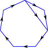
Figure 3. Minimum dilatation digraph.

Properties of the normalized house of reciprocal Perron numbers were recently studied in [McM2], showing that any Perron unit $\alpha$ of degree $n$ satisfies the inequality

$$\alpha^{n}\geq\gamma_{0}^{4},$$

where $\gamma_{0}$ is the golden mean (see Theorem 3.2).

3.4. Complexity of digraphs

The complexity $c$ of a digraph is the number of edges minus the number of vertices of the graph (or minus the topological Euler characteristic).

Lemma 3.1 (Ham-Song [HS]).

If $\lambda$ is the spectral radius of $M$, then $c$ satisfies the inequality

$$c\leq\lambda^{2n}-1.$$

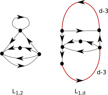
Figure 4. Digraphs realizing $LT_{1,n}$.

Figure 4 shows a family of directed graphs whose characteristic polynomials are given by $LT_{1,3}$. In the Figure, an edge labeled $m$ is subdivided into a chain of $m$ edges and $m-1$ additional vertices. Other examples of digraphs with the same dilatation were found in [Bir]. The ones shown in Figure 4 have the additional property that they are defined from the transition matrix of train track maps associated to pseudo-Anosov mapping classes (see Section 6).

The LT polynomials satisfy

$$|LT_{1,n}|\leq|LT_{a,n}|$$

for all $1\leq a<n$, and for any fixed $0<a$,

$$\lim_{n\rightarrow\infty}|LT_{a,n}|^{2n}=\left(\frac{3+\sqrt{5}}{2}\right)^{2}=\gamma_{0}^{4}.$$

Thus to find the smallest Perron units, it suffices to consider only those with $\lambda<\lambda_{n}=|LT_{1,n}|$. It follows that to solve the minimum dilatation problem it suffices to look at mapping classes whose corresponding digraphs have complexity $c\leq 5$.

3.5. Dilatations of digraphs whose matrices preserve a symplectic form

It is well-known that any Perron number can be realized as the spectral radius of a Perron Frobenius matrix. Furthermore, any Perron unit is the dilatation of a Perron Frobenius matrix that preserves a symplecitc form. It is not known, however, whether every Perron unit is a dilatation of pseudo-Anosov mapping class.

Given a Perron unit $\lambda$, we define its PF-degree to be the minimum dimension of a Perron Frobenius matrix realizing $\lambda$. McMullen has recently announced the following result giving further support to Conjecture 1.1.

Theorem 3.2 (McMullen [McM2]).

Let $p_{d}$ be the minimum Perron unit of Perron degree $d$. Then

1. $(p_{n})^{n}\geq\gamma_{0}^{4}$ for all $n\geq 1$, and

2. $\lim_{n\rightarrow\infty}(p_{n})^{n}=\gamma_{0}^{4}$.

4. Orientable pseudo-Anosov mapping classes

In [LT] Lanneau and Thiffeault studied potential defining polynomials for $\delta_{g}^{+}$ in the cases $g=2,\dots,8$, and found lower bounds for $\delta_{g}^{+}$ for these $g$. Using known examples whose dilatations match these lower bounds they determined $\delta_{g}^{+}$ for $g=2,3,4,5$. From the results of Cho and Ham in [CH], it follows that $\delta_{2}=\delta_{2}^{+}$. Lanneau and Thiffeault’s lower bound for $g=6$ agrees with $\delta_{5}^{+}$, showing that $\delta_{g}^{+}$ is not strictly monotone decreasing. An example realizing $\delta_{7}^{+}$ was found in [AD] and in [KT2], and an example realizing $\delta_{8}^{+}$ was found in [Hir]. The exact value for $\delta_{6}^{+}$ is not known.

The minimum dilatations of orientable pseudo-Anosov mapping classes for low genus are given in Table 2. The associated PF-polynomial is the characteristic polynomial of an associated Perron-Frobenius matrix. This is not necessarily irreducible. In Table 2 we repeatedly see the cyclotomic factor $\sigma(t)=t^{2}-t+1$.

g	$\delta_{g}^{+}\approx$	PF polynomial	factorization
2	1.72208	$t^{4}-t^{3}-t^{2}-t+1$	irreducible
3	1.40127	$t^{8}-t^{7}-t^{4}-t+1$	$\sigma(t)(t^{6}-t^{4}-t^{3}-t^{2}+1)$
4	1.28064	$t^{8}-t^{5}-t^{4}-t^{3}+1$	irreducible
5	1.17628	$t^{12}-t^{7}-t^{6}-t^{5}+1$	$\sigma(t)(t^{10}+t^{9}-t^{7}-t^{6}-t^{5}-t^{4}-t^{3}+t+1)$
7	1.11548	$t^{18}-t^{11}-t^{9}-t^{7}+1$	$\sigma(t)(t^{14}+t^{13}-t^{9}-t^{8}-t^{7}-t^{6}-t^{5}+t+1)$
8	1.12876	$t^{16}-t^{9}-t^{8}-t^{7}+1$	irreducible

Table 2. List of minimum dilatations and their PF polynomials.

For $a,b\in\mathbb{Z}$, define the Lanneau-Thiffeault polynomial $LT_{a,b}$ to be the polynomial

$$LT_{a,b}(t)=t^{2b}-t^{b+a}-t^{b}-t^{b-a}+1.$$

As can be seen from Table 2, for $g=2,3,4,5,7,8$, the PF polynomial for the minimum dilatations of orientable pseudo-Anosov mapping classes is a Lanneau-Thiffeault polynomial.

Question 2.22 can be rephrased as follows.

Question 4.1 (Lanneau-Thiffeault Question).

For even $g\geq 2$ is it true that

$$\delta_{g}^{+}=|LT_{1,g}|$$

where $|LT_{1,g}|$ is the house of $LT_{1,g}(t)$?

By the following result, $|LT_{1,g}|$ is an upper bound for $\delta_{g}^{+}$ for $g$ ranging in an arithmetic sequence or even integers.

Theorem 4.2.

[[Hir]] For each $g\equiv 2,4\pmod{6}$, there is an orientable pseudo-Anosov mapping class on a genus $g$ closed surface with dilatation equal to $|LT_{1,g}|$.

5. Fat train track maps and automata

For each pseudo-Anosov mapping class, one can associate a fat train track map that encodes essential geometric information, including information about singularities, the invariant stable foliation, and dilatations. In this section, we give relevant background and definitions.

5.1. Train tracks and train track maps.

A train track is a finite topological graph $\tau$ (or 1-complex) with no double edges or vertices of degree one. A smoothing of $\tau$ at a vertex $v$ is a choice of tangent directions for the half edges of $\tau$ that meet at $v$, that is if $e_{1}$ and $e_{2}$ meet at a vertex, then they meet either smoothly or in a cusp.

In Figure 5, $e_{3}$ meets $e_{1}$ and $e_{2}$ smoothly, while $e_{1}$ and $e_{2}$ meet at a cusp.

Figure 5. Smoothing at a trivalent vertex

Figure 6 shows a smoothing of a degree four vertex.

Figure 6. Smoothing at a degree 4 vertex

For our examples, we will consider train tracks consisting of a $3b$-gon whose edges meet in cusps and $2b$-edges attached smoothly to the vertices of the $3b$-gon in one of the ways shown in Figure 5 and Figure 6.

By a fat graph, we mean a graph such that at any vertex $v$, there is a cyclic ordering of the half edges that meet at $v$. This gives a local embedding of the half edges meeting at $v$ into a disk centered at $v$. Given any fat graph $\Gamma$, there is a canonical orientable surface $S_{\Gamma}$ with boundary on which $\Gamma$ embeds so that

1. at each vertex the ordering of the edges corresponds to the counterclockwise ordering on the surface; and

2. $S_{\Gamma}$ deformation retracts to the image of $\Gamma$ under the embedding.

Each boundary component is one boundary component of an annular complementary component of $\tau$ on $S_{\Gamma}$. Consider the edges surrounding the other interior boundary component. Each time two adjacent edges meet in a cusp, we call it a vertex of the polygon formed by $\tau$ around the boundary component. If the number of vertices of the polygon is $k$, we say the boundary component is contained in a $k$-gon of $\tau$.

A fat train track $\tau$ embedded on a surface $S$ fills $S$ if $S$ is obtained from $S_{\tau}$ by filling in some subset (possibly empty) of the boundary components of $S_{\tau}$ with disks.

A train track map $f:\tau\rightarrow\tau$ is a local embedding so that vertices map to vertices, and edges map to edge-paths on $\tau$ so that no subinterval of an edge passes across two half edges meeting at a cusp. We consider train track maps up to isotopy on $\tau$.

A train track map $f$ determines a linear transformation $\mathbb{R}^{\mathcal{E}}$ to itself as followis. Let $\mathcal{E}$ be the set of (unoriented) edges of $\tau$. Given $e\in\mathcal{E}$, let

$$f_{*}(e)=\sum_{e^{\prime}}a_{e^{\prime}}e^{\prime},$$

where $a_{e^{\prime}}$ is the number of times $f(e)$ passes over $e^{\prime}$. Define $T:\mathbb{R}^{\mathcal{E}}\rightarrow\mathbb{R}^{\mathcal{E}}$, where for each $w\in\mathbb{R}^{\mathcal{E}}$,

$$T(w)(e)=w(f_{*}(e)),$$

where $w$ extends linearly. The transformation $T$ is called the transition map defined by $f$.

The weight space $W_{\tau}$ of a train track $\tau$ is the subspace of $\mathbb{R}^{\mathcal{E}}$ consisting of edge labels so that if three half edges $e_{1}$, $e_{2}$ and $e_{3}$ meet at a vertex as in Figure 5, then

$$w(e_{1})+w(e_{2})=w(e_{3}),$$

and if $e_{1}$, $e_{2}$, $e_{3}$ and $e_{4}$ meet as in Figure 6, then

$$w(e_{1})+w(e_{2})=w(e_{3})+w(e_{4}).$$

An edge labeling $w$ determines a labeling on edge paths, which we also denote by $w$. Given a train track map $f$ with transition map $T$, we have $T(W_{\tau})=W_{\tau}$.

A train track $\tau\subset S$ and train track map $f:\tau\rightarrow\tau$ is compatible with a mapping class $(S,\phi)$, if $\tau$ fills $S$ and the induced map $\phi_{*}$ on $\tau$ equals $f$.

Theorem 5.1.

If $(S,\phi)$ is pseudo-Anosov, then

1. $(S,\phi)$ has a compatible train track $\tau$ and train track map $f:\tau\rightarrow\tau$;

2. the induced map $f_{*}$ on $W_{\tau}$ is Perron-Frobenius, and preserves a symplectic form; and

3. $\lambda(\phi)$ is the spectral radius of $f_{*}$.

In the examples that follow, it is possible to find a subcollection of edges in $\mathcal{E}$ whose duals in $\mathbb{R}^{\mathcal{E}}$ form a basis for $W_{\tau}$. We call these the real edges of $\tau$ and the complementary set of edges the infinitessimal edges.

5.2. Simplest hyperbolic braid

Figure 7 gives an example of a fat train track and train track map compatible with the simplest hyperbolic braid. The weights in the weight space are determined by their labels on the two longer edges of the train track, and the three encircling loops are the corresponding infinitessimal edges. The action of the simplest hyperbolic braid monodromy defined by $\sigma_{1}\sigma_{2}^{-1}$ acts on the real edges according to the matrix

$$\left[\begin{array}[]{ll}1&1\\ 1&2\end{array}\right],$$

and the dilatation is the largest eigenvalue $\frac{3+\sqrt{5}}{2}=\gamma_{0}^{2}$.

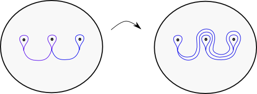
Figure 7. Train track for simplest hyperbolic braid monodromy

5.3. Orientable train tracks

Each train track on $S$ determines a foliation on $S$ as follows. For each complementary region of $\tau$ on $S$ surrounded by a $k$-gon, the foliation has a $k$-pronged singularity. A train track is orientable, if there is an orientation on the edges so that if two edges meet smoothly at a vertex, the orientations are compatible.

Figure 8 sketches the foliation around a boundary component of $S$ corresponding to a hexagon on a fat train track. The orientation on the train track determines an orientation on the foliations.

Thus, we have the following.

Proposition 5.2.

A pseudo-Anosov map $(S,\phi)$ that has a compatible train track map $f:\tau\rightarrow\tau$, where $\tau$ is orientable, is orientable.

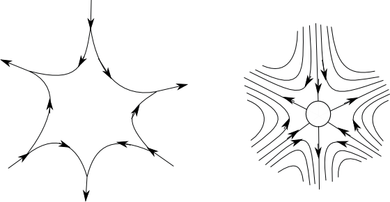
Figure 8. A hexagon on a fat traintrack, and corresponding foliations.

5.4. Train track automaton

Given two fat train tracks $\tau_{1}$ and $\tau_{2}$, a folding map $\mathfrak{f}:\tau_{1}\rightarrow\tau_{2}$ is a quotient map obtained by identifying edge-segments of a pair of edge in $\tau_{1}$ as follows. Take two edges $e_{1}$ and $e_{2}$ on $\tau_{1}$ with half edges that meet at a cusp at a vertex $v$, and that are adjacent in the fat graph ordering. Then the folding map of $e_{1}$ over $e_{2}$ is obtained by identifying the embedded image of a closed interval in $e_{1}$ with endpoint $v$ with $e_{2}$ by a homeomorphism sending $v$ to $v$. The fat train track automaton is the set of all fat train tracks with a directed edge from one train track to another if there is a folding map between them.

Each folding map is a homotopy equivalence of graphs and defines a linear transformation between edge labels, and between weight spaces. A circuit in the fat train track automaton corresponds to a composition of folding maps together with an homeomorphism of train tracks. Thus, the transition matrix for the train track map corresponds to a composition of transition matrices for folding maps and a permutation matrix.

A train track automaton is a directed graph whose vertices are train tracks and edges are folding maps.

Proposition 5.3 (Stallings [Sta], Ham-Song [HS]).

Any pseudo-Anosov mapping class can be represented by a circuit on a train track automaton.

6. Small dilatation examples

In this section, we define train track maps for mapping classes $(S_{n},\phi_{n})$ for all integers $n\geq 2$, and describe corresponding circuits in the train track folding automaton, and digraphs. These train track maps define mapping classes with the same genus, boundary components, and dilatations as $(S_{1,n},\phi_{1,n})$.

We begin with a fat train track map defining $(S_{2},\phi_{2})$ in Figure 9 . One can check that all of the train tracks in the circuit shown in Figure 9 fix a genus two surface with two complementary disk components, one bounded by the central hexagon, and the other bounded by the edges of the hexagon and by each side of the four real edges. The train track map defined by composing the folded mapping classes described in the circuit corresponds to the orientable pseudo-Anoosv mapping classes whose dilatation realizes $\delta_{2}=\delta_{2}^{+}$.

The center hexagon is made up of infinitessimal edges and the other four edges are real edges. Starting at the upper left train track in the the automaton, we first fold edge $a$ over edge $c$ and the following adjacent infinitessimal edge. In the next step we fold $b$ over the new edge $a$. Then we fold the new edge $b$ over $c$. Finally by a rotation, we return to the original train track.

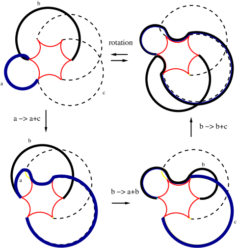
Figure 9. Train track circuit for example realizing $\delta_{2}^{+}$ and $\delta_{2}$.

The transition matrices for the folding diagrams starting at the top left and going around counter-clockwise are:

$$\left[\begin{array}[]{llll}1&0&0&0\\ 0&1&0&0\\ 1&0&1&0\\ 0&0&0&1\end{array}\right]\left[\begin{array}[]{llll}1&1&0&0\\ 0&1&0&0\\ 0&0&1&0\\ 0&0&0&1\end{array}\right]\left[\begin{array}[]{llll}1&0&0&0\\ 0&1&0&0\\ 0&1&1&0\\ 0&0&0&1\end{array}\right]\qquad\mbox{and}\qquad\left[\begin{array}[]{llll}1&0&0&0\\ 0&0&0&1\\ 0&1&0&0\\ 0&0&1&0\end{array}\right].$$

The composition is given by

$$\left[\begin{array}[]{llll}1&1&0&0\\ 0&0&0&1\\ 0&1&0&0\\ 1&1&1&0\\ \end{array}\right]$$

and its characteristic polynomial is $x^{4}-x^{3}-x^{2}-x+1$. This gives

$$\delta_{2}=\delta_{2}^{+}=|x^{4}-x^{3}-x^{2}-x+1|\approx 1.72208.$$

The train track in Figure 9 generalizes to the one in Figure 10.

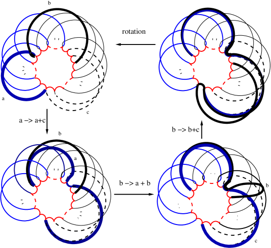
Figure 10. Circuit in train track automaton for $(S_{n},\phi_{n})$

Let $G_{n}$ be the digraphs in Figure 4. The “shape” of the train track map and folding maps for $(S_{n},\phi_{n})$ are related to each other in a systematic way, and one observes the following.

Proposition 6.1.

The digraphs associated to the transition matrices for the train track maps of $(S_{n},\phi_{n})$ are $G_{n}$, and hence the dilatations of $(S_{n},\phi_{n})$ are given by

$$\lambda(\phi_{n})=|LT_{1,n}|.$$

The genus of $S_{n}$ can be determined from the topological Euler characteristic of $G_{n}$, $\chi(G_{n})=2n$ and the number of boundary components of the fat graph. There is one component for the central $3n$-gon, and either one or three other boundary components, depending on whether $n$ is divisible by 3. This implies the following.

Proposition 6.2.

The surface $S_{n}$ has genus $g=n$ if $n=1,2\pmod{3}$, and has genus $g=n-1$ if $n=0\pmod{3}$.

From the train track maps, we can also determine when the mapping classes are orientable, for this is exactly when the train tracks themselves are orientable as seen in the next proposition.

Proposition 6.3.

The mapping class $(S_{n},\phi_{n})$ is orientable if and only if $n$ is even.

Proof.

The complementary region of $(S_{n},\phi_{n})$ splits into a central $3n$-gon and either one $n$-gon, or three $n/3$-gons, depending on whether or not $n$ is divisible by 3. In order for the train track to be orientable, we need to have each polygon have an even number of sides. Thus, $n$ must be even.

When $n$ is even, there are two possible ways to orient the central $3n$-gon. Each extends to a compatible orientation on the entire train track. (An example is shown in Figure 11).

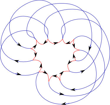
Figure 11. Oriented train track for $n=4$.

Remark 6.4.

In [LT], it is shown that the mapping class on a closed genus 2 surface with minimum dilatation is unique up to standard equivalences. Thus, the mapping class described in Figure 9 is the same as the genus 2 monodromy of the complement of the link drawn in Figure 2. In a forthcoming paper, we will further elaborate on the construction shown in this section.

Department of Mathematics, Florida State University, 1017 Academic Way, Tallahassee, FL 32306-4510. email: hironaka$@$math.fsu.edu

References

- [AD] J. Aaber and N. Dunfield. Closed surface bundles of least volume. Algebr. Geom. Topology 10 (2010), 2315–2342.
- [Bir] J. Birman. On pseudo-Anosov mapping classes with minimum dilatation and Lanneau-Thiffeault numbers. arxiv:1101.2383v1 (2011).
- [CB] A. Casson and S. Bleiler. Automorphisms of surfaces after Nielsen and Thurston. Cambridge University Press, 1988.
- [CH] J. Cho and J. Ham. The minimal dilatation of a genus two surface. Experiment. Math. 17 (2008), 257–267.
- [Dob] E. Dobrowolski. On a question of Lehmer and the number of irreducible factors of a polynomial. Acta. Arith. 34 (1979), 391–401.
- [FLM] B. Farb, C. Leininger, and D. Margalit. Small dilatation pseudo-Anosovs and 3-manifolds. Adv. Math 228 (2011), 1466–1502.
- [FLP] A. Fathi, F. Laudenbach, and V. Poénaru. Some dynamics of pseudo-Anosov diffeomorphisms. In Travaux de Thurston sur les surfaces, volume 66-67 of Astérisque. Soc. Math. France, Paris, 1979.
- [Fri] D. Fried. Flow equivalence, hyperbolic systems and a new zeta function for flows. Comment. Math. Helvetici 57 (1982), 237–259.
- [Gor] C. Gordon. Small surfaces and Dehn filling. In Proceedings of the Kirbyfest (Berkeley, CA, 1998), volume 2, pages 177–199. Coventry, 1999.
- [HS] J-Y Ham and W. T. Song. The minimum dilatation of pseudo-Anosov 5-braids. Experimental Mathematics 16 (2007), 167,180.
- [Hir] E. Hironaka. Small dilatation pseudo-Anosov mapping classes coming from the simplest hyperbolic braid. Algebr. Geom. Topol. 10 (2010), 2041–2060.
- [HK] E. Hironaka and E. Kin. A family of pseudo-Anosov braids with small dilatation. Algebr. Geom. Topol. 6 (2006), 699–738.
- [KT1] E. Kin and M. Takasawa. Pseudo-Anosov braids with small entropy and the magic 3-manifold. Comm. Anal. Geo. 19 (2011), 705–758.
- [KT2] E. Kin and M. Takasawa. Pseudo-Anosovs on closed surfaces having small entropy and the Whitehead sister link exterior. J. Math. Soc. Japan 65 (2013), 411–446.
- [Kit] B. Kitchens. Symbolic dynamics: one-sided, two-sided and countable state Markov shifts. Springer, 1998.
- [KKT] S. Kojima, E. Kin, and M. Takasawa. Minimal dilatations of pseudo-Anosovs generated by the magic 3-manifold and their asymptotic behavior. Algebraic and Geometric Topology 13 (2013), 3537–3602.
- [LT] E. Lanneau and J.-L. Thiffeault. On the minimum dilatation of pseudo-Anosov homeomorphisms on surfaces of small genus. Ann. de l’Inst. Four. 61 (2009), 164–182.
- [Leh] D. H. Lehmer. Factorization of certain cyclotomic functions. Ann. of Math. 34 (1933), 461–469.
- [McM1] C. McMullen. Polynomial invariants for fibered 3-manifolds and Teichmüller geodesics for foliations. Ann. Sci. École Norm. Sup. 33 (2000), 519–560.
- [McM2] C. McMullen. Entropy and the clique polynomial. Preprint (2013).
- [Pen] R. Penner. Bounds on least dilatations. Proceedings of the A.M.S. 113 (1991), 443–450.
- [Rolf] D. Rolfsen. Knots and Links. Publish or Perish, Inc, Berkeley, 1976.
- [Smy] C. J. Smyth. On the product of the conjugates outside the unit circle of an algebraic integer. Bull. London Math. Soc. 3 (1971), 169–175.
- [Sta] J. R. Stallings. Topology of finite graphs. Invent. Math. 71 (1983), 551–565.
- [Sun] H. Sun. A transcendental invariant of pseudo-Anosov maps. preprint (2012).
- [Thu1] W. Thurston. A norm for the homology of 3-manifolds. Mem. Amer. Math. Soc. 339 (1986), 99–130.
- [Thu2] W. Thurston. On the geometry and dynamics of diffeomorphisms of surfaces. Bull. Amer. Math. Soc. (N.S.) 19 (1988), 417–431.
- [Thu3] W. Thurston. arXiv:1402.2008 [math.DS] (2014).