Dalitz plot studies of $D^{0}\to K^{0}_{S}\pi^{+}\pi^{-}$ decays in a factorization approach

Abstract

The presently available high-statistics data of the $D^{0}\to K^{0}_{S}\pi^{+}\pi^{-}$ processes measured by the Belle and BABAR Collaborations are analyzed within a quasi two-body factorization framework. Starting from the weak effective Hamiltonian, tree and annihilation amplitudes build up the $D^{0}\to K^{0}_{S}\pi^{+}\pi^{-}$ decay amplitude. Two of the three final-state mesons are assumed to form a single scalar, vector or tensor state originating from a quark-antiquark pair so that the factorization hypothesis can be applied. The meson-meson final state interactions are described by $K\pi$ and $\pi\pi$ scalar and vector form factors for the $S$ and $P$ waves and by relativistic Breit-Wigner formulae for the $D$ waves. A combined $\chi^{2}$ fit to a Belle Dalitz plot density distribution, to the total experimental branching fraction and to the $\tau^{-}\to K^{0}_{S}\pi^{-}\nu_{\tau}$ decay data is carried out to fix the 33 free parameters. These are mainly related to the strengths of the scalar form factors and to unknown meson to meson transition form factors at a large momentum transfer squared equal to the $D^{0}$ mass squared. A good overall agreement to the Belle Dalitz plot density distribution is achieved. Another set of parameters fits equally well the BABAR Collaboration Dalitz plot model. The parameters of both fits are close, following from similar Dalitz density distribution data for both collaborations. The corresponding one-dimensional effective mass distributions display the contributions of the ten quasi two-body channels entering our $D^{0}\to K^{0}_{S}\pi^{+}\pi^{-}$ decay amplitude. The branching fractions of the dominant channels compare well with those of the isobar Belle or BABAR models. The lower-limit values of the branching fractions of the annihilation amplitudes are significant. Built upon experimental data from other processes, the unitary $K\pi$ and $\pi\pi$ scalar form factors, entering our decay amplitude and satisfying analyticity and chiral symmetry constraints, are furthermore constrained by the present Dalitz plot analysis. Our $D^{0}\to K^{0}_{S}\pi^{+}\pi^{-}$ decay amplitude could be a useful input for determinations of $D^{0}$-$\overline{D}^{0}$ mixing parameters and of the CKM angle $\gamma$ (or $\phi_{3}$).

I Introduction

Measurements of the $D^{0}$-$\overline{D}^{0}$ mixing parameters, through Dalitz-plot time dependent amplitude analyses of the the weak process $D^{0}\to K^{0}_{S}\pi^{+}\pi^{-}$, have been performed by the Belle ZhangPRL99_131803 and BABAR SanchezPRL105_081803 Collaborations. These studies could help in the understanding of the origin of mixing and may indicate the possible presence of new physics contribution. No $CP$ violation in these $D^{0}$ decays D.M.AsnerPRD70_0911018CLEO ; T.Aaltonen_CDF2012 has yet been found, in agreement with the very small value predicted by the standard model in the charm sector. The Cabibbo-Kobayashi-Maskawa, CKM, angle $\gamma$ (or $\phi_{3}$) has been evaluated from the analyses of the $B^{\pm}\to D^{0}K^{\pm},D^{0}\to K^{0}_{S}\pi^{+}\pi^{-}$ decays J.Libby_PRD82_CLEO ; R.Aaij_LHCb2012 ; H.Aihara_Belle2012 ; SanchezPRL105121801 ; J.P.Lees_PRD87_052015_BABAR ; A.Poluektov_PRD81_112002_Belle . A good knowledge of the final state meson interactions is important to reduce the uncertainties in the determination of the $D^{0}$-$\overline{D}^{0}$ mixing parameters and of the angle $\gamma$. The very rich structures seen in the Dalitz plot spectra point out to the complexity of these final state strong interactions.

The experimental analyses ZhangPRL99_131803 ; SanchezPRL105_081803 rely mainly on the use of the isobar model. In this approach one can take into account the many existing resonances coupled to the interacting pairs of mesons. However, the corresponding decay amplitudes are not unitary and unitarity is not preserved in the three-body decay channels; it is also violated in the two-body sub-channels. Furthermore, it is difficult to differentiate the $S$-wave amplitudes from the non-resonant background terms. Their interferences are noteworthy and then some two-body branching fractions, extracted from the data, could be unreliable. The isobar model is tractable but it has many free parameters: at least two fitted parameters for each amplitude and for example, the Belle Collaboration in Ref. ZhangPRL99_131803 has used 40 fitted parameters and BABAR Collaboration 43 in Ref. SanchezPRL105_081803 .

Imposing unitarity for three-body strong interactions in a wide range of meson-meson effective masses is difficult. Some three-body unitarity corrections have been evaluated in Ref. KamanoPRD84 for $D^{0}\to\pi^{0}\pi^{+}\pi^{-}$ decays and in Ref. MagalhaesPRD84 for $D^{+}\rightarrow K^{-}\pi^{+}\pi^{+}$. In a unitary coupled-channel model Ref. KamanoPRD84 has shown that two-body rescattering terms could be important. They find that the decay amplitudes of the unitary model can be rather different from those of the isobar model. In Ref. MagalhaesPRD84 the three-body unitarity is formulated with an integral equation inspired by the Faddeev formalism. There, they sum up a perturbation series and find that three-body effects important close to threshold fade away at higher energies. In the present work, as a first step, we require two-body unitarity in the $D$-decay amplitudes with $K^{0}_{S}\pi^{\pm}$ final state in $S$ wave and with the $\pi^{+}\pi^{-}$ final state in $S$ and $P$ waves. According to the experimental works ZhangPRL99_131803 ; SanchezPRL105_081803 , the sum of the branching fractions corresponding to these amplitudes yields an important part of the total branching fraction of the $D^{0}\rightarrow K^{0}_{S}\pi^{+}\pi^{-}$ decay.

The two-body QCD factorization has been applied with success to charmless nonleptonic $B$ decays  (see e.g. Ref. Beneke2003 ). For the $D$ meson the charm quark mass $m_{c}$ is lighter than the bottom quark mass by about a factor of three. The $c$ quark mass is too high to apply chiral perturbation theory and too light to use heavy quark expansion approaches. One expects nonperturbative $D$-decay contributions of order $\Lambda_{QCD}/m_{c}$ to be more important than in $B$ decays. Consequently the factorization hypothesis could be less reliable. Nevertheless, following the initial articles of Bauer, Stech and Wirbel Wirbel1985 ; Bauer1987 the assumption of factorization has been applied successfully to $D$ decays in several recent papers BoitoPRD79_034020 ; El-Bennich_PRD79 ; BoitoPRD80_054007 ; Fu-Sheng_Yu_PRD84_074019 . The Wilson coefficients are treated as phenomenological parameters to account for possible important non-factorizable corrections BurasNPB434_606 . An alternative diagrammatic approach for the description of hadronic charmed meson decays into two body has been the support of the works presented in Refs. ChengPRD81_074021 and ChengPRD81_074031 .

In the framework of the quasi two-body factorization approximation Beneke2003 and of the extension of a program devoted to the understanding of rare three-body $B$ decays fkll ; El-Bennich2006 ; Bppk ; Leitner_PRD81 ; DedonderPol we analyze the presently available $D^{0}\to K^{0}_{S}\pi^{+}\pi^{-}$ data. So far no factorization scheme has been worked out for three-body decays. Then, as in our previous studies, we assume that two of the three final-state mesons forms a single state which originates from a quark-antiquark, $q\bar{q}$, pair. Such an hypothesis leads to quasi two-body final states to which the factorization procedure is applied. The three-meson final states $K^{0}_{S}\pi^{+}\pi^{-}$ are here supposed to be formed by the following quasi two-body pairs, $[K^{0}_{S}\pi^{+}]_{L}\ \pi^{-}$, $[K^{0}_{S}\pi^{-}]_{L}\ \pi^{+}$ and $K^{0}_{S}\ [\pi^{+}{\pi^{-}}]_{L}$ where two of the three mesons form a state in $L=S,P$ or $D$ wave. The $D^{0}\to K^{0}_{S}\pi^{+}\pi^{-}$ decay amplitudes, derived from the weak effective Hamiltonian, have contributions from tree diagrams but none from penguin or $W$-loop diagrams. There are also annihilation amplitudes arising from $W$-meson exchange between the $D^{0}$ quark constituents. The amplitudes corresponding to the $c\to su\bar{d}$ transition are Cabibbo favored (CF) while those with $c\to du\bar{s}$ are doubly Cabibbo suppressed (DCS).

In the factorization approach, the CF and DCS amplitudes are expressed as superpositions of appropriate effective coefficients and two products of two transition matrix elements. For the CF tree amplitudes, the first and second product correspond to the transition matrix element between the $D^{0}$ and $[\overline{K}^{0}\pi^{-}]_{L}$ or $[\pi^{+}\pi^{-}]_{L}$ state multiplied by the transition matrix element between the vacuum and the $\pi^{+}$ (proportional to the pion decay constant) or the $\overline{K}^{0}$ (proportional to the kaon decay constant), respectively. For the DCS tree amplitude these products correspond to the transition between the $D^{0}$ and $\pi^{-}$ or $[\pi^{-}\pi^{+}]_{L}$ state multiplied by the transition between the vacuum and the $[K^{0}\pi^{+}]_{L}$ (proportional to the kaon-pion form factor) or the ${K}^{0}$ (proportional to the kaon decay constant), respectively. In the latter case, in the $K^{0}\pi$ center of mass frame, the bilinear quark current involved forces the $[K^{0}\pi^{+}]$ pair to be in a $L=S$ or $P$ wave. For the CF (DCS) annihilation amplitudes the products correspond to the transition between the $\pi$ or $\overline{K}^{0}$(${K}^{0}$) and $[\overline{K}^{0}\pi^{-}]_{L}$($[{K}^{0}\pi^{+}]_{L}$) or $[\pi^{+}\pi^{-}]_{L}$ state, multiplied by the transition between the vacuum and the $D^{0}$ (proportional to the $D^{0}$ decay constant), respectively.

We presume that the transition of the $D^{0}$ to the meson pairs $[\overline{K}^{0}\pi^{-}]_{L}$ or $[\pi^{+}\pi^{-}]_{L}$ goes first through the dominant intermediate resonance $R_{L}$ of these pairs. For the $[\overline{K}^{0}\pi^{-}]_{L}$ pair, we take, $R_{S}[\overline{K}^{0}\pi^{-}]=K^{*}_{0}(1430)^{-}$, $R_{P}[\overline{K}^{0}\pi^{-}]=K^{*}(892)^{-}$, $R_{D}[\overline{K}^{0}\pi^{-}]=K^{*}_{2}(1430)^{-}$ and for the $[\pi^{+}\pi^{-}]_{L}$ pair, $R_{S}[\pi^{+}\pi^{-}]=f_{0}(980)$, $R_{P}[\pi^{+}\pi^{-}]=\rho(770)^{0}$ and $R_{D}[\pi^{+}\pi^{-}]=f_{2}(1270)$. We further calculate the $D^{0}\to\overline{K}^{0}\pi^{-}$ or $\pi^{+}\pi^{-}$ matrix elements as products of the $D^{0}\to R_{L}[\overline{K}^{0}\pi^{-}]$ or $R_{L}[\pi^{+}\pi^{-}]$ transition form factors by the relevant vertex function describing the decay of the $[\overline{K}^{0}\pi]_{L}$ or $[\pi\pi]_{L}$ states into the final meson pair. The vertex functions are in turn expected to be proportional to the kaon-pion or pion scalar form factor for the $S$ wave, to the vector form factor for the $P$ wave and to a relativistic Breit-Wigner formula for the $D$ wave. For the CF (DCS) annihilation amplitudes we follow the same steps as for the tree amplitudes but for the replacement of $D^{0}$ by $\pi$ or $\overline{K}^{0}$(${K}^{0}$).

The meson-meson final state interactions for the $S$ and $P$ waves are then described in terms of experimentally and theoretically constrained $K\pi$ and $\pi\pi$ scalar and vector form factors. Using unitarity, analyticity and chiral symmetry constraints, the scalar form factors have been been derived in Ref. Bppk for the $K\pi$ case and in Ref. DedonderPol for the pion one. They are single unitary functions describing the two scalar resonances $K^{*}_{0}(800)$ (or $\kappa$), $K^{*}_{0}(1430)$ and the three scalar resonances, $f_{0}(500)$, $f_{0}(980)$ and $f_{0}(1400)$ present in the $K^{0}_{S}\pi^{\pm}$ and $\pi^{+}\pi^{-}$ interactions, respectively. The vector form factors are based on the Belle analyses of the $\tau^{-}\to K^{0}_{S}\pi^{-}\nu_{\tau}$  EpifanovPLB654 and of the $\tau^{-}\to\pi^{-}\pi^{0}\nu_{\tau}$ Belletau2008 decay processes. We also include the amplitude describing the $D^{0}\to\omega(782)K^{0}_{S}$ channel followed by the $\omega(782)\to\pi^{+}\pi^{-}$ decay. Relativistic Breit-Wigner formulae are introduced to describe the final state $D$ wave meson-meson interactions. The undetermined parameters of our $D^{0}\to K^{0}_{S}\pi^{+}\pi^{-}$ decay amplitudes, mainly related to the strength of the $[{K}\pi]_{S}$ and $[\pi\pi]_{S}$ scalar form factors and to the unknown meson to meson transition form factors, are obtained through a $\chi^{2}$ fit to the Dalitz plot data sample of the 2010 Belle Collaboration analysis A.Poluektov_PRD81_112002_Belle ; A.Poluektov_private2013 . We also fit the Dalitz plot density of the BABAR Collaboration model F.Martinez_private2013 .

The paper is structured as follows. Section II describes formally the amplitudes calculated in the framework of the quasi two-body factorization approach. Section III provides a practical formulation of these amplitudes by introducing combinations of some of them more amenable to numerical calculations. A discussion of the branching fractions is also given there. Section IV lists the necessary input for the evaluation of the amplitudes. Results are presented and discussed in Section V while Section VI summarizes the outcome of this analysis and proposes some conclusions and perspectives.

II The $D^{0}\to K^{0}_{S}\pi^{+}\pi^{-}$ decay amplitudes in factorization framework

The decay amplitudes for the $D^{0}\to K^{0}_{S}\pi^{+}\pi^{-}$ process can be evaluated as matrix elements of the effective weak Hamiltonian Buchalla1996

$$H_{eff}=\frac{G_{F}}{\sqrt{2}}V_{CKM}\Big{[}C_{1}(\mu)O_{1}(\mu)+C_{2}(\mu)O_{2}(\mu)\Big{]}+h.c.,$$ (1)

where the coefficients $V_{CKM}$ are given in terms of Cabibbo-Kobayashi-Maskawa quark-mixing matrix elements and $G_{F}$ denotes the Fermi coupling constant. The $C_{i}(\mu)$ are the Wilson coefficients of the four-quark operators $O_{i}(\mu)$ at a renormalization scale $\mu$, chosen to be equal to the $c$-quark mass $m_{c}$. The left-handed current-current operators $O_{1,2}(\mu)$ arise from $W$-boson exchange.

The transition matrix elements that occur in the present work require two specific values of the $V_{CKM}$ coupling matrix elements:

$$\Lambda_{1}\equiv V^{*}_{cs}V_{ud}\hskip 28.45274pt{\rm and}\hskip 28.45274pt\Lambda_{2}\equiv V^{*}_{cd}V_{us}.$$ (2)

The amplitudes are functions of the Mandelstam invariants

$$s_{\pm}=m_{\pm}^{2}=(p_{0}+p_{\pm})^{2},\hskip 56.9055pts_{0}=m_{0}^{2}=(p_{+}+p_{-})^{2},$$ (3)

where $p_{0}$, $p_{+}$ and $p_{-}$ are the four-momenta of the $K_{S}^{0}$, $\pi^{+}$ and $\pi^{-}$ mesons, respectively. Energy-momentum conservation implies

$$p_{D^{0}}=p_{0}+p_{+}+p_{-}\hskip 28.45274pt{\rm and}\hskip 28.45274pts_{0}+s_{+}+s_{-}=m_{D^{0}}^{2}+m_{K^{0}}^{2}+2m_{\pi}^{2},$$ (4)

where $p_{D^{0}}$ is the $D^{0}$ four-momentum and $m_{D^{0}}$, $m_{K^{0}}$ and $m_{\pi}$ denote the $D^{0}$, $K^{0}$ and charged pion masses.

The full amplitude is the superposition of two tree Cabibbo favored and doubly Cabibbo suppressed amplitudes, $T^{CF}(s_{0},s_{-},s_{+})$ and $T^{DCS}(s_{0},s_{-},s_{+})$ and of two annihilation (i.e., exchange of W meson between the $c$ and $\overline{u}$ quarks of the $D^{0}$) CF and DCS amplitudes, $A^{CF}(s_{0},s_{-},s_{+})$ and $A^{DCS}(s_{0},s_{-},s_{+})$. Thus, one writes the full amplitude as

$$\mathcal{M}(s_{0},s_{-},s_{+}) = \left\langle K^{0}_{S}(p_{0})\ \pi^{+}(p_{+}){\pi^{-}}(p_{-})|H_{eff}|D^{0}(p_{D^{0}})\right\rangle$$ (5)

$$= T^{CF}(s_{0},s_{-},s_{+})+T^{DCS}(s_{0},s_{-},s_{+})+A^{CF}(s_{0},s_{-},s_{+})+A^{DCS}(s_{0},s_{-},s_{+}),$$

where the CF amplitudes are proportional to $\Lambda_{1}$ and the DCS ones to $\Lambda_{2}$. Although the three variables $s_{0},s_{-},s_{+}$ appear as arguments of the amplitudes, because of the relation (4) all amplitudes depend only on two of them.

Assuming that the factorization approach Beneke2003 ; BurasNPB434_606 ; Buchalla1996 ; AliPRD58 with quasi two-body $[K\pi]_{L}\pi$ or $K[\pi\pi]_{L},L=S,P,D$, states holds, the tree CF amplitudes read, with $|0\rangle$ indicating the vacuum state,

$$T^{CF}(s_{0},s_{-},s_{+}) \simeq \frac{G_{F}}{2}\ \Lambda_{1}\sum_{L={S,P,D}}\Big{[}a_{1}(m_{c})\langle[\overline{K}^{0}(p_{0}){\pi^{-}}(p_{-})]_{L}|(\overline{s}\ c)_{V-A}|D^{0}(p_{D^{0}})\rangle$$ (6)

$$\cdot\ \langle\pi^{+}(p_{+})|(\overline{u}\ d)_{V-A}|0\rangle+a_{2}(m_{c})\langle\overline{K}^{0}(p_{0})|(\overline{s}\ d)_{V-A}|0\rangle$$

$$\cdot\ \langle[\pi^{+}(p_{+}){\pi^{-}}(p_{-})]_{L}|(\overline{u}\ c)_{V-A}|D^{0}(p_{D^{0}})\rangle\Big{]}$$

$$= \sum_{L={S,P,D}}T^{CF}_{[\overline{K}^{0}\pi^{-}]_{L}\pi^{+}}(s_{0},s_{-},s_{+})+\sum_{L={S,P,D}}T^{CF}_{\overline{K}^{0}[\pi^{+}\pi^{-}]_{L}}(s_{0},s_{-},s_{+})$$

$$= T^{CF}_{[\overline{K}^{0}\pi^{-}]\pi^{+}}(s_{0},s_{-},s_{+})+T^{CF}_{\overline{K}^{0}[\pi^{+}\pi^{-}]}(s_{0},s_{-},s_{+}).$$

In deriving Eq. (6) small $CP$ violation effects in $K^{0}_{S}$ decays are neglected and we use

$$|K^{0}_{S}\rangle\approx\frac{1}{\sqrt{2}}\ \left(|K^{0}\rangle+|\overline{K}^{0}\rangle\right).$$ (7)

At leading order in the strong coupling constant $\alpha_{S}$, the effective QCD factorization coefficients $a_{1}(m_{c})$ and $a_{2}(m_{c})$ are expressed as

$$a_{1}(m_{c})=C_{1}(m_{c})+\frac{C_{2}(m_{c})}{N_{C}},\hskip 28.45274pta_{2}(m_{c})=C_{2}(m_{c})+\frac{C_{1}(m_{c})}{N_{C}},$$ (8)

where $N_{C}=3$ is the number of colors. Higher order vertex and hard scattering corrections are not discussed in the present work and we introduce effective values for these coefficients (see Sec. IV). From now on, the simplified notation $a_{1}\equiv a_{1}(m_{c})$ and $a_{2}\equiv a_{2}(m_{c})$ will be used. In Eq. (6), we have introduced the short-hand notation

$$(\overline{q}\ q)_{V-A}=\overline{q}\gamma\ (1-\gamma_{5})\ q$$ (9)

which will be used throughout the text. The amplitudes $T^{CF}_{[\overline{K}^{0}\pi^{-}]\ \pi^{+}}(s_{0},s_{-},s_{+})$ and $T^{CF}_{\overline{K}^{0}\ [\pi^{+}\pi^{-}]}(s_{0},s_{-},s_{+})$ are illustrated diagrammatically in Figs. 1 and 2.

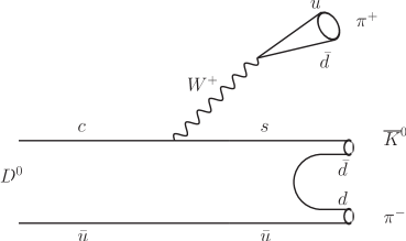
Figure 1: Tree diagram for Cabibbo favored amplitudes with $\left[\overline{K}^{0}\pi^{-}\right]\pi^{+}$ final states.

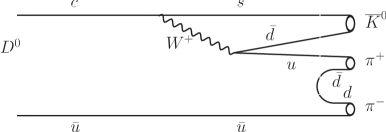
Figure 2: As in Fig. 1 but for $\overline{K}^{0}\left[\pi^{+}\pi^{-}\right]$ final states.

Similarly, the DCS tree amplitudes, illustrated by the diagrams shown in Figs. 3 and 4, read

$$T^{DCS}(s_{0},s_{-},s_{+}) \simeq \frac{G_{F}}{2}\ \Lambda_{2}\sum_{L={S,P,D}}\Big{[}a_{1}\langle[K^{0}(p_{0})\pi^{+}(p_{+})]_{L}|(\overline{u}\ s)_{V-A}|0\rangle$$ (10)

$$\cdot\ \langle\pi^{-}(p_{-}))|(\overline{d}\ c)_{V-A}|D^{0}(p_{D^{0}})\rangle+a_{2}\langle K^{0}(p_{0})|(\overline{d}\ s)_{V-A}|0\rangle$$

$$\cdot\ \langle[\pi^{+}(p_{+})\pi^{-}(p_{-})]_{L}|(\overline{u}\ c)_{V-A}|D^{0}(p_{D^{0}})\rangle\Big{]}$$

$$= \sum_{L={S,P,D}}T^{DCS}_{[{K}^{0}\pi^{+}]_{L}\pi^{-}}(s_{0},s_{-},s_{+})+\sum_{L={S,P,D}}T^{DCS}_{{K}^{0}[\pi^{-}\pi^{+}]_{L}}(s_{0},s_{-},s_{+})$$

$$= T^{DCS}_{[{K}^{0}\pi^{+}]\pi^{-}}(s_{0},s_{-},s_{+})+T^{DCS}_{{K}^{0}[\pi^{-}\pi^{+}]}(s_{0},s_{-},s_{+}).$$

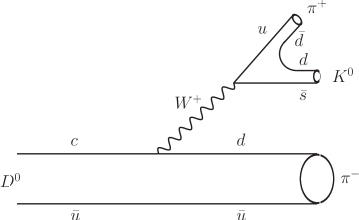
Figure 3: Tree diagram for the doubly Cabibbo suppressed amplitude with $\left[{K}^{0}\pi^{+}\right]\pi^{-}$ final states.

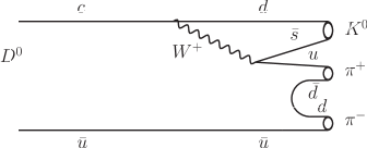
Figure 4: As in Fig. 3 but for ${K}^{0}\left[\pi^{+}\pi^{-}\right]$ final states.

A similar derivation for the CF annihilation amplitudes, illustrated by the diagram in Fig. 5, yields

$$A^{CF}(s_{0},s_{-},s_{+}) \approx \frac{G_{F}}{2}\ \Lambda_{1}\ a_{2}\sum_{L={S,P,D}}\left[\langle[\overline{K}^{0}(p_{0})\pi^{-}(p_{-})]_{L}\ \pi^{+}(p^{+})|(\overline{s}\ d)_{V-A}|0\rangle\right.$$ (11)

$$+ \left.\langle\overline{K}^{0}(p_{0})\ [\pi^{-}(p_{-})\pi^{+}(p^{+})]|(\overline{s}\ d)_{V-A}|0\rangle\right]\cdot\langle 0|(\overline{c}\ u)_{V-A}|D^{0}(p_{D^{0}})\rangle$$

$$= \sum_{L={S,P,D}}A^{CF}_{[\overline{K}^{0}\pi^{-}]_{L}\pi^{+}}(s_{0},s_{-},s_{+})+\sum_{L={S,P,D}}A^{CF}_{\overline{K}^{0}[\pi^{+}\pi^{-}]_{L}}(s_{0},s_{-},s_{+})$$

$$= A^{CF}_{[\overline{K}^{0}\pi^{-}]\pi^{+}}(s_{0},s_{-},s_{+})+A^{CF}_{\overline{K}^{0}[\pi^{+}\pi^{-}]}(s_{0},s_{-},s_{+}).$$

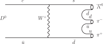
Figure 5: Diagram for the Cabibbo favored annihilation ($W$-exchange) amplitudes.

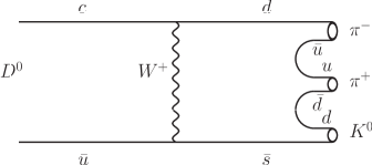
Figure 6: As in Fig. 5 but for the doubly Cabibbo suppressed annihilation ($W$-exchange) amplitudes.

The corresponding DCS annihilation amplitudes (see Fig. 6), obtained from Eq. (11) with the substitutions $\Lambda_{1}\Longrightarrow\Lambda_{2}$, $\pi^{+}\Longleftrightarrow\pi^{-}$, $\overline{K}^{0}\Longrightarrow K^{0}$ and $d\Longleftrightarrow s$, read

$$A^{DCS}(s_{0},s_{-},s_{+}) \approx \frac{G_{F}}{2}\ \Lambda_{2}\ a_{2}\sum_{L={S,P,D}}\left[\langle[K^{0}(p_{0})\pi^{+}(p_{+})]_{L}\ \pi^{-}(p^{-})|(\overline{d}\ s)_{V-A}|0\rangle\right.$$ (12)

$$+ \left.\langle K^{0}(p_{0})\ [\pi^{+}(p_{+})\pi^{-}(p^{-})]|(\overline{d}\ s)_{V-A}|0\rangle\right]\cdot\langle 0|(\overline{c}\ u)_{V-A}|D^{0}(p_{D^{0}})\rangle$$

$$= \sum_{L={S,P,D}}A^{DCS}_{[{K}^{0}\pi^{+}]_{L}\pi^{-}}(s_{0},s_{-},s_{+})+\sum_{L={S,P,D}}A^{DCS}_{{K}^{0}[\pi^{-}\pi^{+}]_{L}}(s_{0},s_{-},s_{+})$$

$$= A^{DCS}_{[{K}^{0}\pi^{+}]\pi^{-}}(s_{0},s_{-},s_{+})+A^{DCS}_{{K}^{0}[\pi^{-}\pi^{+}]}(s_{0},s_{-},s_{+}).$$

Let us now review in detail the 28 amplitudes that build up the total $D^{0}~{}\to~{}K^{0}_{S}\pi^{+}\pi^{-}$ amplitude defined in Eq. (5). Indeed, for each amplitude in Eq. (5) there are three ($L=S$, $P$, $D$) contributions for the $[K\pi]\pi$ states and three for the $K[\pi\pi]$ ones as can be seen from Eqs. (6), (10)-(12). To these 24 amplitudes one has to add the four contributions in which the $[\pi\pi]_{P}$ pair in the $K[\pi\pi]$ final state originates from the $\omega(782)\to\pi^{+}\pi^{-}$ decay.

II.1 Cabibbo favored amplitudes

The $[K_{S}^{0}\pi^{-}]_{S}\ \pi^{+}$ and $K_{S}^{0}\ [\pi^{+}\pi^{-}]_{S}$ amplitudes

Starting from Eq. (6) we build now the expression of the different CF amplitudes following a derivation similar to that described in details in Ref. DedonderPol (see, in particular, Appendix A of Ref. DedonderPol and Sec. II.3 of this paper where an analogous explicit derivation for the annihilation amplitudes is presented). The $[K_{S}^{0}\pi^{-}]_{S}\ \pi^{+}$ amplitude is

$$T^{CF}_{[\overline{K}^{0}\pi^{-}]_{S}\ \pi^{+}}(s_{0},s_{-},s_{+}) = -\frac{G_{F}}{2}\ a_{1}\Lambda_{1}\ \chi_{1}\ \left(m_{D^{0}}^{2}-s_{-}\right)\ f_{\pi}\ F_{0}^{D^{0}R_{S}[\overline{K}^{0}\pi^{-}]}(m_{\pi}^{2})\ F_{0}^{\overline{K}^{0}\pi^{-}}(s_{-})$$ (13)

$$\equiv T_{1}.$$

The transition form factor $F_{0}^{D^{0}R_{S}[\overline{K}^{0}\pi^{-}]}(m_{\pi}^{2})$ is dominated by the $K_{0}^{*}(1430)^{-}$ resonance. It is real in the kinematical range considered here. The form factor $F_{0}^{\overline{K}^{0}\pi^{-}}(s_{-})$ includes the contribution of the $K_{0}^{*}(800)^{-}$ (or $\kappa^{-})$ and $K_{0}^{*}(1430)^{-}$ resonances.

The $K_{S}^{0}\ [\pi^{+}\pi^{-}]_{S}$ amplitude reads

$$T^{CF}_{\overline{K}^{0}\ [\pi^{+}\pi^{-}]_{S}}(s_{0},s_{-},s_{+}) = -\frac{G_{F}}{2}\ a_{2}\ \Lambda_{1}\ \chi_{2}\ (m_{D^{0}}^{2}-s_{0})\ f_{K^{0}}\ F_{0}^{D^{0}R_{S}[\pi^{+}\pi^{-}]}(m_{K^{0}}^{2})\ F_{0}^{\pi^{+}\pi^{-}}(s_{0})$$ (14)

$$\equiv T_{2},$$

where the transition form factor $F_{0}^{D^{0}R_{S}[\pi^{+}\pi^{-}]}(m_{K^{0}}^{2})$ is assumed to be dominated by the $f_{0}(980)$ resonance. It is also purely real.

In the equations above, $f_{\pi}$ and $f_{K^{0}}$ represent the pion and $K^{0}$ decay constants. The [$\pi\pi$] $S$-wave form factor $F_{0}^{\pi^{+}\pi^{-}}(s_{0})$ includes the contribution of the $f_{0}(500)$ (or $\sigma),f_{0}(980)$ and $f_{0}(1400)$ resonances. The $K\pi$ and $\pi\pi$ scalar form factors $F_{0}^{\overline{K}^{0}\pi^{-}}(s_{-})$ and $F_{0}^{\pi^{+}\pi^{-}}(s_{0})=\sqrt{\frac{2}{3}}\ \Gamma^{n*}_{1}(s_{0})$ will be built following the methods discussed in Refs. Bppk and DedonderPol .

In Eqs. (13) and (14) the factors $\chi_{1}$ and $\chi_{2}$ are related to the strength of the $[K\pi]_{S}$ and $[\pi\pi]_{S}$ scalar form factors, respectively. As just mentioned these form factors receive contributions from different resonances. If a resonance $R_{S}[K\pi]$ or $R_{S}[\pi\pi]$ was dominant $\chi_{1}$ and $\chi_{2}$ could be evaluated in terms of the decay constant of these resonances. As shown in Eq. (A.8) of Ref. DedonderPol and as discussed in Sec. V of the present paper, their values could be estimated from the dominating resonance decay properties. Here, there is no dominant resonance then $\chi_{1}$ and $\chi_{2}$ are taken as complex constants to be fitted.

The $[K_{S}^{0}\pi^{-}]_{P}\ \pi^{+}$ and $K_{S}^{0}\ [\pi^{+}\pi^{-}]_{P}$ amplitudes

The $[K_{S}^{0}\pi^{-}]_{P}\ \pi^{+}$ amplitude reads, with $K^{*-}\equiv K^{*}(892)^{-}$,

$$T^{CF}_{[\overline{K}^{0}\pi^{-}]_{P}\ \pi^{+}}(s_{0},s_{-},s_{+}) = \frac{G_{F}}{2}\ a_{1}\ \Lambda_{1}\ \frac{f_{\pi}}{f_{{K^{*-}}}}\left(s_{0}-s_{+}+(m_{K^{0}}^{2}-m_{\pi}^{2})\ \frac{m_{D^{0}}^{2}-m_{\pi}^{2}}{s_{-}}\right)$$ (15)

$$\times\ A_{0}^{D^{0}R_{P}[\overline{K}^{0}\pi^{-}]}(m_{\pi}^{2})\ F_{1}^{\overline{K}^{0}\pi^{-}}(s_{-})\equiv T_{3},$$

where $A_{0}^{D^{0}R_{P}[\overline{K}^{0}\pi^{-}]}(m_{\pi}^{2})$ denotes the form factor describing the $D^{0}$ to $[\overline{K}^{0}\pi^{-}]_{P}$ transition, largely dominated by the $K^{*}(892)^{-}$ resonance. The form factor $F_{1}^{\overline{K}^{0}\pi^{-}}(s_{-})$ includes a priori the contribution of the $K^{*}(892)^{-}$, $K_{1}(1410)^{-}$ and $K^{*}(1680)^{-}$ resonances EpifanovPLB654 (see Sec. IV). It has been discussed notably in Refs. Bppk , mouss2008 and  BoitoEPJC .

The $K_{S}^{0}\ [\pi^{+}\pi^{-}]_{P}$ amplitude is given by

$$T^{CF}_{\overline{K}^{0}\ [\pi^{+}\pi^{-}]_{P}}(s_{0},s_{-},s_{+})=\frac{G_{F}}{2}\ a_{2}\ \Lambda_{1}\ \frac{f_{K^{0}}}{f_{{\rho}}}\ (s_{-}-s_{+})\ A_{0}^{D^{0}R_{P}[\pi^{+}\pi^{-}]}(m_{K^{0}}^{2})\ F_{1}^{\pi^{+}\pi^{-}}(s_{0})\equiv T_{4},$$ (16)

where the transition form factor $A_{0}^{D^{0}\\ R_{P}[\pi^{+}\pi^{-}]}(m_{K^{0}}^{2})$ is dominated by the $\rho(770)^{0}$ resonance. The form factor $F_{1}^{\pi^{+}\pi^{-}}(s_{0})$ which includes a priori the contributions of the $\rho(770)^{0}$, $\rho(1450)^{0}$ and $\rho(1700)^{0}$ is the same as that introduced in Ref. DedonderPol , following the analysis in Ref. Belletau2008 based on a Gounaris-Sakurai form with parameters extracted from third column of their Table VII. Alternatively we also use one of the unitary parametrizations derived by Hanhart in Ref. Hanhart . Since the $K^{*-}$ and $\rho(770)^{0}$ are dominating resonances, we use in Eqs. (15) and (16), $f_{{K^{*-}}}$ and $f_{{\rho}}$ to represent the $R_{P}{[\overline{K}^{0}\pi^{-}]}$ and $R_{P}{[\pi^{+}\pi^{-}]}$ decay constants (here, $f_{\rho}$ denotes the charged $\rho$ decay constant).

The $D^{0}\to\overline{K}^{0}[\pi^{+}\pi^{-}]_{P}$ decay can also proceed through the two-step process $D^{0}\to\overline{K}^{0}\ \omega$ followed by the decay $\omega\to\pi^{+}\pi^{-}$; it yields an amplitude similar to that of the $D^{0}\to\overline{K}^{0}\ [\pi^{+}\pi^{-}]_{P}$ process with the replacement of the $[\pi^{+}\pi^{-}]_{P}$ pair by the $\omega$ and the subsequent decay $\omega\to\pi^{+}\pi^{-}$, which violates isospin conservation. Thus, this term has to be added to the $P$-wave amplitude. Defining

$$\langle\overline{K}^{0}(p_{0})\ [\pi^{+}(p_{+})\pi^{-}(p_{-})]_{\omega}|H_{eff}|D^{0}(p_{D})\rangle=T^{CF}_{\overline{K}^{0}[\pi^{+}\pi^{-}]_{\omega}}(s_{0},s_{-},s_{+}),$$ (17)

one has, in the quasi two-body factorization,

$$T^{CF}_{\overline{K}^{0}[\pi^{+}\pi^{-}]_{\omega}}(s_{0},s_{-},s_{+}) = \frac{G_{F}}{\sqrt{2}}\ \Lambda_{1}\ a_{2}\ \langle\overline{K}^{0}(p_{0})|(\overline{s}d)_{V-A}|0\rangle$$ (18)

$$\cdot\ \langle[\pi^{+}(p_{+})\pi^{-}(p_{-})]_{\omega}|(\overline{u}c)_{V-A}|D^{0}(p_{D^{0}})\rangle$$

with

$$\langle\overline{K}^{0}(p_{0})|(\overline{s}d)_{V-A}|0\rangle=i\ f_{K^{0}}\ p_{0},$$ (19)

and

$$\langle[\pi^{+}(p_{+})\pi^{-}(p_{-})]_{\omega}|(\overline{u}c)_{V-A}|D^{0}(p_{D^{0}})\rangle = \frac{1}{\sqrt{2}}\ G_{\omega\pi^{+}\pi^{-}}(s_{0})\ \epsilon\cdot(p^{+}-p^{-})$$ (20)

$$\times \ \langle\omega(p_{+}+p_{-})|\ (\overline{u}c)_{V-A}|D^{0}(p_{D^{0}})\rangle.$$

where $\epsilon$ represents the four-vector polarization of the $\omega$ meson. The matrix element in the above equation reads (see, e.g., Eq. (24) of Ref. AliPRD58 )

$$\langle\omega(s_{0})|\ (\overline{u}c)_{V-A}|D^{0}(p_{D^{0}})\rangle=-i\ \frac{2\ m_{\omega}\ (\epsilon^{*}\cdot p_{D})}{p_{0}^{2}}\ p_{0}\ A_{0}^{D^{0}\omega}(p_{0}^{2})+{\rm``other\ terms"},$$ (21)

where the “other terms” do not contribute when they are multiplied by Eq. (19). The $\omega\pi^{+}\pi^{-}$ vertex function is given by

$$G_{\omega\pi^{+}\pi^{-}}(p_{+}+p_{-})=\frac{g_{\omega\pi\pi}}{m_{\omega}^{2}-s_{0}-i\ m_{\omega}\ \Gamma_{\omega}},$$ (22)

where the expression of the coupling coefficient $g_{\omega\pi\pi}$ is given in Sec. IV and $\Gamma_{\omega}$ is the $\omega$ total width. One eventually arrives at

$$T^{CF}_{\overline{K}^{0}\ [\pi^{+}\pi^{-}]_{\omega}}(s_{0},s_{-},s_{+})=\frac{G_{F}}{2}\ a_{2}\ \Lambda_{1}\ \frac{f_{K^{0}}}{\sqrt{2}}\ m_{\omega}\ (s_{-}-s_{+})\ \frac{g_{\omega\pi\pi}\ A_{0}^{D^{0}\omega}(m_{K^{0}}^{2})}{m_{\omega}^{2}-s_{0}-i\ m_{\omega}\ \Gamma_{\omega}}\equiv T_{5}.$$ (23)

The $[K_{S}^{0}\pi^{-}]_{D}\ \pi^{+}$ and $K_{S}^{0}\ [\pi^{+}\pi^{-}]_{D}$ amplitudes

One has finally to evaluate the $[K_{S}^{0}\pi^{-}]_{D}\ \pi^{+}$ amplitude associated to the $K_{2}^{*-}\equiv K_{2}^{*-}(1430)$ resonance for the $[K_{S}^{0}\pi^{-}]_{D}$ states and the $K_{S}^{0}\ [\pi^{+}\pi-]_{D}$ one related to the $f_{2}\equiv f_{2}(1270)$ for the $[\pi^{+}\pi^{-}]_{D}$ states. With the notation $m_{K_{2}^{*}}\equiv m_{K_{2}^{*-}(1430)}$, the amplitude related to the $K_{2}^{*-}$ resonance reads

$$T^{CF}_{[{\overline{K}^{0}}\pi^{-}]_{D}\ \pi^{+}}(s_{0},s_{-},s_{+}) = -\frac{G_{F}}{2}\ a_{1}\ \Lambda_{1}\ f_{\pi}\ F^{{D^{0}}R_{D}[\overline{K}^{0}\pi^{-}]}(s_{-},m_{\pi}^{2})\ \frac{g_{K_{2}^{*-}K^{0}_{S}\pi^{-}}\ D(\bf{p_{1}},\bf{p_{+}})}{m_{K_{2}^{*}}^{2}-s_{-}-i\ m_{K_{2}^{*}}\ \Gamma_{K_{2}^{*}}}$$ (24)

$$\equiv T_{6},$$

where $g_{K_{2}^{*-}K_{S}^{0}\pi^{-}}$ is the $K_{2}^{*-}$ coupling constant to the ${{K}^{0}_{S}}\pi^{-}$ pair since the width $\Gamma_{K_{2}^{*}}$ will be considered as constant [see Eqs. (123)-(125)]. The function $D({\bf{p_{1}}},{\bf p_{+}})$ is expressed in terms of the momenta in the $[{{K}^{0}_{S}}\pi^{-}]$ center-of-mass system defined in Appendix A

$$D({\bf p_{1}},{\bf p_{+}})=\frac{1}{3}\ (|{\bf p_{1}}|\ |{\bf p_{+}}|)^{2}-({\bf p_{1}}\cdot{\bf p_{+}})^{2}.$$ (25)

The transition form factor $F^{D^{0}R_{D}[\overline{K}^{0}\pi^{-}]}(s_{-},m_{\pi}^{2})$ follows from Ref. KimPRD67 (see their Eq. (10a)), and depends on three distinct functions of the four momentum transfer squared at $m_{\pi}^{2}$, $k^{D^{0}K_{2}^{*-}}(m_{\pi}^{2})$, $b^{D^{0}K_{2}^{*-}}_{+}(m_{\pi}^{2})$ and $b^{D^{0}K_{2}^{*-}}_{-}(m_{\pi}^{2})$, such that

$$F^{{D^{0}}R_{D}[\overline{K}^{0}\pi^{-}]}(s_{-},m_{\pi}^{2})=k^{D^{0}K_{2}^{*-}}(m_{\pi}^{2})+b^{D^{0}K_{2}^{*-}}_{+}(m_{\pi}^{2})\ (m_{D^{0}}^{2}-s_{-})+b^{D^{0}K_{2}^{*-}}_{-}(m_{\pi}^{2})\ m_{\pi}^{2}.$$ (26)

For the amplitude related to the $f_{2}$ meson with mass $m_{f_{2}}\equiv m_{f_{2}(1270)}$ one has

$$T^{CF}_{\overline{K}^{0}\ [\pi^{+}\pi^{-}]_{D}}(s_{0},s_{-},s_{+}) = -\frac{G_{F}}{2}\ a_{2}\ \Lambda_{1}\ \frac{f_{K^{0}}}{\sqrt{2}}\ F^{D^{0}R_{D}[\pi^{+}\pi^{-}]}(s_{0},m_{K^{0}}^{2})\ \frac{g_{f_{2}\pi^{+}\pi^{-}}\ D({\bf p_{2}},{\bf p_{0}})}{m_{f_{2}}^{2}-s_{0}-i\ m_{f_{2}}\ \Gamma_{f_{2}}(s_{0})}$$ (27)

$$\equiv T_{7},$$

where $g_{f_{2}\pi^{+}\pi^{-}}$ characterizes the strength of the $f_{2}\to\pi^{+}\pi^{-}$ transition [see Eqs. (119) and (120)]. Here, because of the rather large width of the $f_{2}$ meson, the total width $\Gamma_{f_{2}}(s_{0})$ depends on the invariant mass squared $s_{0}$. The function $D({\bf p_{2}},{\bf p_{0}})$ is given by the same expression as in Eq. (25) replacing ${\bf p_{1}}$ by ${\bf p_{2}}$ and ${\bf p_{+}}$ by ${\bf p_{0}}$, the corresponding momenta and scalar product defined in Eqs. (131)-(133). In Eq. (27), the $D^{0}$ to $f_{2}$ transition form factor, $F^{D^{0}R_{D}[\pi^{+}\pi^{-}]}(s_{0},m_{K^{0}}^{2})$ depends on three distinct functions of the four momentum transfer squared at $m_{K^{0}}^{2}$

$$F^{D^{0}R_{D}[\pi^{+}\pi^{-}]}(s_{0},m_{K^{0}}^{2})=k^{D^{0}f_{2}}(m_{K^{0}}^{2})+b_{+}^{D^{0}f_{2}}(m_{K^{0}}^{2})\ (m_{D^{0}}^{2}-s_{0})+b_{-}^{D^{0}f_{2}}(m_{K^{0}}^{2})\ m_{K^{0}}^{2}.$$ (28)

II.2 The doubly Cabibbo suppressed amplitudes

To the Cabbibo favored amplitudes of the preceding subsection must now be added the doubly Cabibbo suppressed tree amplitudes which are derived from Eq. (10) in a similar way to that used for the CF amplitudes. For the $[K^{0}_{S}\pi^{+}]_{S}\pi^{-}$ amplitude, we have

$$T^{DCS}_{[{K^{0}}\pi^{+}]_{S}\ \pi^{-}}(s_{0},s_{-},s_{+})=\frac{G_{F}}{2}\ a_{1}\ \Lambda_{2}\ (m_{D^{0}}^{2}-m_{\pi}^{2})\ \frac{m_{K^{0}}^{2}-m_{\pi}^{2}}{s_{+}}\ F_{0}^{D^{0}{\pi^{-}}}(s_{+})\ F_{0}^{K^{0}\pi^{+}}(s_{+})\equiv T_{8},$$ (29)

while the $K^{0}_{S}[\pi^{-}\pi^{+}]_{S}$ amplitude reads

$$T^{DCS}_{K^{0}\ [\pi^{-}\pi^{+}]_{S}}\ (s_{0},s_{-},s_{+})=\frac{\Lambda_{2}}{\Lambda_{1}}\ T^{CF}_{\overline{K}^{0}\ [\pi^{+}\pi^{-}]_{S}}(s_{0},s_{-},s_{+})=\frac{\Lambda_{2}}{\Lambda_{1}}\ T_{2}.$$ (30)

For the $[K^{0}_{S}\pi^{+}]_{P}\ \pi^{-}$ amplitude we obtain

$$T^{DCS}_{[{K^{0}}\pi^{+}]_{P}\ \pi^{-}}(s_{0},s_{-},s_{+}) = -\frac{G_{F}}{2}\ a_{1}\ \Lambda_{2}\ \left[s_{0}-s_{-}+(m_{D^{0}}^{2}-m_{\pi}^{2})\ \frac{m_{K^{0}}^{2}-m_{\pi}^{2}}{s_{+}}\right]$$ (31)

$$\times\ F_{1}^{D^{0}\pi^{-}}(s_{+})\ F_{1}^{K^{0}\pi^{+}}(s_{+})\equiv T_{9}.$$

For the $K^{0}_{S}\ [\pi^{-}\pi^{+}]_{P}$ amplitude, one has two contributions, associated mainly to the $\rho(770)^{0}$ and to the $\omega(782)$. They read

$$T^{DCS}_{{K}^{0}\ [\pi^{-}\pi^{+}]_{P}}(s_{0},s_{-},s_{+})=\frac{\Lambda_{2}}{\Lambda_{1}}\ T^{CF}_{{\overline{K}}^{0}\ [\pi^{+}\pi^{-}]_{P}}(s_{0},s_{-},s_{+})=\frac{\Lambda_{2}}{\Lambda_{1}}\ T_{4}$$ (32)

and

$$T^{DCS}_{{K^{0}}\ [\pi^{-}\pi^{+}]_{\omega}}(s_{0},s_{-},s_{+})=\frac{\Lambda_{2}}{\Lambda_{1}}\ T^{CF}_{\overline{K}^{0}\ [\pi^{+}\pi^{-}]_{\omega}}(s_{0},s_{-},s_{+})=\frac{\Lambda_{2}}{\Lambda_{1}}\ T_{5},$$ (33)

respectively. Associated to the $[K\pi]$ and $[\pi\pi]$ $D$- states, there is only one non-zero amplitude, that related to the $f_{2}$ meson,

$$T^{DCS}_{{K^{0}}\ [\pi^{-}\pi^{+}]_{D}}(s_{0},s_{-},s_{+})=\frac{\Lambda_{2}}{\Lambda_{1}}\ T^{CF}_{\overline{K}^{0}\ [\pi^{+}\pi^{-}]_{D}}(s_{0},s_{-},s_{+})=\frac{\Lambda_{2}}{\Lambda_{1}}\ T_{7}.$$ (34)

No contribution comes from the $[K\pi]$ $D$-wave since one has $<0|(\overline{u}\ s)_{V-A}|K_{2}^{*+}>=0,$ so that

$$T^{DCS}_{[{K}^{0}\pi^{+}]_{D}\ \pi^{-}}(s_{0},s_{-},s_{+})\propto T_{10}=0.$$ (35)

The expressions of the CF and DCS “emission” amplitudes of the $D^{0}$ to pseudoscalar-vector meson decays, given in the Appendix of Ref. Fu-Sheng_Yu_PRD84_074019 , agree with our CF [see Eqs. (15), (16), (23)] and DCS [see Eqs. (31)-(33)] tree amplitudes for the dominant resonance $K^{*}(892)$, $\rho(770)^{0}$ and $\omega$ part, respectively.

II.3 The annihilation ($W$-exchange) Cabibbo favored amplitudes

Let us sketch a systematic derivation for these amplitudes defined in Eq. (11) and illustrated diagrammatically by Fig. 5 (see, e.g., Sec. V.C in Ref. AliPRD58 ). Denoting by $M_{1}(p_{1})$ and $M_{2}(p_{2})$ the quasi two-meson final state, we may write, in the quasi two-body factorization, for the CF amplitudes

$$\langle M_{1}(p_{1})M_{2}(p_{2})|H_{eff}|D^{0}(p_{D^{0}})\rangle = \frac{G_{F}}{\sqrt{2}}\ a_{2}\ \Lambda_{1}\ \langle M_{1}(p_{1})M_{2}(p_{2})|(\overline{s}d)_{V-A}|0\rangle$$ (36)

$$\cdot\ \langle 0|(\overline{u}c)_{V-A}|D^{0}(p_{D^{0}})\rangle$$

The second term in the right hand side of Eq. (36) corresponds to the annihilation of the $D^{0}$ that goes through the W exchange between the $c\overline{u}$ quark pair that builds the $D^{0}$ (see Ref. AliPRD58 ). In Eq. (36) the possible quasi-two-meson pairs are (see Eq. (11)):

$$M_{1}(p_{0}+p_{-})\equiv[\overline{K}^{0}(p_{0})\pi^{-}(p_{-})]_{L},\hskip 56.9055ptM_{2}(p_{+})\equiv\pi^{+}(p_{+}),$$ (37)

$$M_{1}(p_{+}+p_{-})\equiv[\pi^{+}(p_{+})\pi^{-}(p_{-})]_{L},\hskip 56.9055ptM_{2}(p_{0})\equiv\overline{K}^{0}(p_{0}).$$ (38)

The meson pairs are assumed to originate from a pair of quarks: a $s\overline{u}$ pair in the first case and a $d\overline{d}$ one in the second. For the $D^{0}$ decay constant, $f_{D^{0}}$ one takes (the phase is chosen in accordance with the choice made in Eq. (A.3) of Ref. DedonderPol )

$$\langle 0|(\overline{u}\ c)_{V-A}|D^{0}(p_{D^{0}})\rangle=-i\ f_{D^{0}}\ p_{D^{0}}.$$ (39)

Thus, all annihilation amplitudes will be proportional to the $D^{0}$ decay constant $f_{D^{0}}$. The form factor $\langle M_{1}(p_{1})M_{2}(p_{2})|(\overline{s}d)_{V-A}|0\rangle$ is evaluated in terms of the transition form factors between the pseudoscalar $M_{2}(-p_{2})$ and the meson pair $[m_{1}(p_{3})m_{2}(p_{4})]_{L}$ in scalar, vector or tensor state, with respective four-momenta $p_{3}$ and $p_{4}$. We introduce the hypothesis that the transitions of the pseudoscalar meson $M_{2}(-p_{2})$ to the $[m_{1}(p_{3})m_{2}(p_{4})]_{L}$ states go through intermediate resonances $M_{1}(p_{1})$ where the four-momentum $p_{1}$ fulfills the energy-momentum conservation relation $p_{1}~{}=~{}p_{3}~{}+~{}p_{4}$; these intermediate resonances then decay into the $[m_{1}(p_{3}),m_{2}(p_{4})]$ pairs. In the case of Eq. (37) one identifies $m_{1}(p_{3})$ with the $\overline{K}^{0}$ meson with four momentum $p_{0}$ and $m_{2}(p_{4})$ with the $\pi^{-}$ meson with four-momentum $p_{-}$ whereas, in the case of Eq. (38) one identifies $m_{1}(p_{3})$ with the $\pi^{+}$ meson with four momentum $p_{+}$ and $m_{2}(p_{4})$ with the $\pi^{-}$ meson with four-momentum $p_{-}$. The resonance decays are described by vertex functions $G_{R_{L}[m_{1}m_{2}]}(p_{1}^{2})$ modeled assuming them to be proportional to the scalar $R_{S}[m_{1}m_{2}]$ or vector $R_{P}[m_{1}m_{2}]$ form factor for the $S$ and $P$ amplitudes or to a relativistic Breit-Wigner function for the $R_{D}[m_{1}m_{2}]$ states. The model thus yields the following contributions.

For $[m_{1}m_{2}]_{S}$ waves

$$<M_{1}(p_{1})M_{2}(p_{2})| \!\!(\overline{s}d)_{V-A}\!\! |0>=G_{R_{S}[m_{1}m_{2}]}(s_{34})\ \langle R_{S}[m_{1}(p_{3})m_{2}(p_{4})]|(\overline{s}d)_{V-A}|M_{2}(-p_{2})\rangle$$ (40)

$$= \!\!-i\ G_{R_{S}[m_{1}m_{2}]}(s_{34})\ \Big{\{}\big{[}-p_{2}+p_{3}+p_{4}+\frac{p_{2}^{2}-(p_{3}+p_{4})^{2}}{m_{D^{0}}^{2}}\ p_{D^{0}}\big{]}\$$

$$\times \!\!F_{1}^{M_{2}R_{S}[m_{1}m_{2}]}(m_{D^{0}}^{2})-\frac{p_{2}^{2}-(p_{3}+p_{4})^{2}}{m_{D^{0}}^{2}}\ p_{D^{0}}\ F_{0}^{M_{2}R_{S}[m_{1}m_{2}]}(m_{D^{0}}^{2})\Big{\}}\!,$$

where $F_{0}^{M_{2}R_{S}[m_{1}m_{2}]}(m_{D^{0}}^{2})$ and $F_{1}^{M_{2}R_{S}[m_{1}m_{2}]}(m_{D^{0}}^{2})$ denote the $M_{2}R_{S}[m_{1}m_{2}]$ scalar and vector form factors. The vertex function $G_{R_{S}[m_{1}m_{2}]}(s_{34})$ is modeled according to

$$G_{R_{S}[m_{1}m_{2}]}(s_{34})=\chi_{R_{S}[m_{1}m_{2}]}\ F_{0}^{m_{1}m_{2}}(s_{34}),\hskip 28.45274pt{\rm with}\hskip 28.45274pts_{34}=p_{1}^{2}=(p_{3}+p_{4})^{2},$$ (41)

$F_{0}^{m_{1}m_{2}}(s_{34})$ being the $[m_{1}m_{2}]$ scalar form factor and $\chi_{R_{S}[m_{1}m_{2}]}$ characterizing the strength of the $S$-state form factor contribution as discussed in Sec. II.1. With $\chi_{R_{S}[\overline{K}^{0}\pi^{-}]}\equiv\chi_{1}$ [see Eq. (13)] the CF $[\overline{K}^{0}(p^{0})\pi^{-}(p_{-})]_{S}\ \pi^{+}(p_{+})$ annihilation amplitude is

$$A^{CF}_{[\overline{K}^{0}\pi^{-}]_{S}\ \pi^{+}}(s_{0},s_{-},s_{+}) = -\frac{G_{F}}{2}\ a_{2}\ \Lambda_{1}\ \chi_{1}\ (m_{\pi}^{2}-s_{-})\ f_{D^{0}}\ F_{0}^{\pi^{+}R_{S}[\overline{K}^{0}\pi^{-}]}(m_{D^{0}}^{2})\ F_{0}^{\overline{K}^{0}\pi^{-}}(s_{-})$$ (42)

$$\equiv A_{1}.$$

For the $[\pi^{+}(p_{+})\pi^{-}(p_{-})]_{S}$ pair, we have, with $\chi_{R_{S}[\pi^{+}\pi^{-}]}\equiv\chi_{2}$, [see Eq.  (14)],

$$A^{CF}_{\overline{K}^{0}\ [\pi^{+}\pi^{-}]_{S}}(s_{0},s_{-},s_{+}) = -\frac{G_{F}}{2}\ a_{2}\ \Lambda_{1}\ \chi_{2}\ (m_{K^{0}}^{2}-s_{0})\ f_{D^{0}}\ F_{0}^{\overline{K}^{0}R_{S}[\pi^{+}\pi^{-}]}(m_{D^{0}}^{2})\ F_{0}^{\pi^{+}\pi^{-}}(s_{0})$$ (43)

$$\equiv A_{2}.$$

Since the $D^{0}$ mass is larger than the masses of the two-meson thresholds $m_{\pi}+m_{K_{0}^{*}(800)}$ and $m_{\overline{K}^{0}}+m_{f_{0}(500)}$, the transition form factors $F_{0}^{\pi^{+}R_{S}[\overline{K}^{0}\pi^{-}]}(m_{D^{0}}^{2})$ and $F_{0}^{\overline{K}^{0}R_{S}[\pi^{+}\pi^{-}]}(m_{D^{0}}^{2})$ appearing in these equations are unknown complex parameters to be fitted.

For the $[m_{1}m_{2}]_{P}$ wave contributions, denoting for simplicity the vector meson resonances as

$$V_{R}\equiv R_{P}[m_{1}m_{2}],$$

we may write

$$\langle[m_{1}(p_{3})m_{2}(p_{4})]_{P}\ M_{2}(p_{2})|(\overline{d}s)_{V-A}|0\rangle=G_{V_{R}}(p_{1}^{2})\ \epsilon\cdot(p_{3}-p_{4})\ \langle V_{R}(p_{1}^{2})|(\overline{s}d)_{V-A}|M_{2}(-p_{2})\rangle,$$ (44)

$\epsilon$ being the polarization of the vector resonance and $G_{V_{R}}$ the $V_{R}$ decay vertex function. One has AliPRD58

$$\langle V_{R}(p_{1}^{2})|(\overline{s}d)_{V-A}|M_{2}(-p_{2})\rangle=-i\ \frac{2m_{V_{R}}\ (\epsilon^{*}\cdot p_{2})}{p^{2}_{D^{0}}}\ p_{D^{0}}\ A_{0}^{M_{2}V_{R}}(m_{D^{0}}^{2})+{\rm``other\ terms"}.$$ (45)

Here $p_{D^{0}}=p_{1}+p_{2}$. The “other terms” do not contribute when multiplying the matrix element (45) by that of Eq. (39). The $P$ states being characterized by dominant resonances, one writes

$$G_{V_{R}}(p_{1}^{2})=\frac{1}{m_{V_{R}}\ f_{V_{R}}}\ F_{1}^{m_{1}m_{2}}(p_{1}^{2}),$$

where $f_{V_{R}}$ is the $V_{R}$ decay constant. One thus arrives at the following expressions

$$A^{CF}_{[\overline{K}^{0}\pi^{-}]_{P}\ \pi^{+}}(s_{0},s_{-},s_{+}) = -\frac{G_{F}}{2}\ a_{2}\ \Lambda_{1}\ \frac{f_{D^{0}}}{f_{K^{*-}}}\left[s_{0}-s_{+}+\frac{(m_{D^{0}}^{2}-m_{\pi}^{2})(m_{K^{0}}^{2}-m_{\pi}^{2})}{s_{-}}\right]$$ (46)

$$\times\ A_{0}^{\pi^{+}R_{P}[\overline{K}^{0}\pi^{-}]}(m_{D^{0}}^{2})\ F_{1}^{\overline{K}^{0}\pi^{-}}(s_{-})\equiv A_{3},$$

and

$$A^{CF}_{\overline{K}^{0}\ [\pi^{+}\pi^{-}]_{P}}(s_{0},s_{-},s_{+}) = \frac{G_{F}}{2}\ a_{2}\ \Lambda_{1}\ \frac{f_{D^{0}}}{f_{\rho}}\ (s_{-}-s_{+})\ A_{0}^{\overline{K}^{0}R_{P}[\pi^{+}\pi^{-}]}(m_{D^{0}}^{2})\ F_{1}^{\pi^{+}\pi^{-}}(s_{0})$$ (47)

$$\equiv A_{4},$$

and, if the $[\pi^{-}\pi^{+}]_{P}$ originates from the $\omega$ resonance,

$$A^{CF}_{\overline{K}^{0}\ [\pi^{+}\pi^{-}]_{\omega}}(s_{0},s_{-},s_{+})=-\frac{G_{F}}{2}\ a_{2}\ \Lambda_{1}\ \frac{f_{D^{0}}}{\sqrt{2}}\ m_{\omega}\ (s_{-}-s_{+})\ \frac{g_{\omega\pi\pi}\ A_{0}^{\overline{K}^{0}[\pi^{+}\pi^{-}]_{\omega}}(m_{D^{0}}^{2})}{m_{\omega}^{2}-s_{0}-i\ m_{\omega}\ \Gamma_{\omega}}\equiv A_{5},$$ (48)

Since we are in the $\overline{K}^{0}V_{R}$ scattering region, the values of the form factors $A_{0}^{\overline{K}^{0}R_{P}[\pi^{+}\pi^{-}]}(m_{D^{0}}^{2})$ and $A_{0}^{\overline{K}^{0}[\pi+\pi^{-}]_{\omega}}(m_{D^{0}}^{2})$ are complex numbers.

Finally, for the $[m_{1}m_{2}]_{D}$ wave contributions, denoting for simplicity the tensor meson resonances as

$$T_{R}\equiv T_{R}[m_{1}m_{2}]$$

and the polarization tensor of the D-wave resonance as $\mathbf{\epsilon}_{\alpha\beta}(\lambda)$, $\lambda$ being the spin projection, one can write

$$\langle[m_{1}(p_{3})m_{2}(p_{4})]_{D}\ M_{2}(p_{2})|\ (\overline{s}d)_{V-A}|0\rangle = G_{T_{R}}(p_{1}^{2})\$$ (49)

$$\times\ \sum_{\lambda=-2}^{\lambda=+2}\epsilon_{\alpha\beta}(\lambda)\ p_{3}^{\alpha}\ p_{4}^{\beta}\ \langle T_{R}^{\lambda}(p_{1}^{2})\ M_{2}(-p_{2})|(\overline{s}d)_{V-A}|0\rangle.$$

Reformulating the matrix element for the $M_{2}\ T_{R}$ to vacuum transition

$$-i\ f_{D^{0}}\ p_{D^{0}}\cdot\langle T_{R}^{\lambda}(p_{1}^{2})\ M_{2}(p_{2})|(\overline{s}d)_{V-A}|0\rangle=f_{D^{0}}\ F^{M_{2}T_{R}}(p_{1}^{2},m_{D^{0}}^{2})\ \epsilon^{*}_{\mu\nu}(\lambda)\ p_{2}^{\nu}\ p_{2}^{\mu}.$$ (50)

where (see Ref. KimPRD67 )

$$-i\ F^{M_{2}T_{R}}(p_{1}^{2},m_{D^{0}}^{2})=k^{M_{2}T_{R}}(m_{D^{0}}^{2})+b_{+}^{M_{2}T_{R}}(m_{D^{0}}^{2})\ (m_{M_{2}}^{2}-p_{1}^{2})+b_{-}^{M_{2}T_{R}}(m_{D^{0}}^{2})\ m_{D^{0}}^{2}.$$ (51)

Here, $k^{M_{2}T_{R}}$, $b_{+}^{M_{2}T_{R}}$ and $b_{-}^{M_{2}T_{R}}$ are complex transition form factors since $m_{D^{0}}^{2}>(m_{M_{2}}+m_{T_{R}})^{2}$. Assuming then, for these cases, Breit-Wigner representations of the resonance vertex functions $G_{T_{R}}(p_{1}^{2})$ and summing over the spin projections $\lambda$, one arrives at the following expressions

$$A^{CF}_{[\overline{K}^{0}\pi^{-}]_{D}\ \pi^{+}}(s_{0},s_{-},s_{+}) = \frac{G_{F}}{2}\ a_{2}\ \Lambda_{1}\ f_{D^{0}}\ F^{R_{D}[\overline{K}^{0}\pi^{-}]\pi^{+}}(s_{-},m_{D^{0}}^{2})$$ (52)

$$\times\ g_{K_{2}^{*-}K^{0}_{S}\pi^{-}}\ \frac{D({\bf p_{1}},{\bf p_{+}})}{m_{K_{2}^{*}}^{2}-s_{-}-i\ m_{K_{2}^{*}}\ \Gamma_{K_{2}^{*}}}\equiv A_{6},$$

$$A^{CF}_{\overline{K}^{0}\ [\pi^{+}\pi^{-}]_{D}}(s_{0},s_{-},s_{+}) = \frac{G_{F}}{2}\ a_{2}\ \Lambda_{1}\ \frac{f_{D^{0}}}{\sqrt{2}}\ F^{\overline{K}^{0}R_{D}[\pi^{+}\pi^{-}]}(s_{0},m_{D^{0}}^{2})$$ (53)

$$\times\ g_{f_{2}\pi^{+}\pi^{-}}\ \frac{D({\bf p_{2}},{\bf p_{0}})}{m_{f_{2}}^{2}-s_{0}-i\ m_{f_{2}}\ \Gamma_{f_{2}}(s_{0})}\equiv A_{7},$$

where the expressions of $g_{K_{2}^{*-}K^{0}_{S}\pi^{-}}$, $g_{f_{2}\pi^{+}\pi^{-}}$ and of the resonance widths are discussed in Sect. IV.

II.4 The annihilation ($W$-exchange) doubly Cabibbo suppressed amplitudes

One has to evaluate the corresponding Cabbibo suppressed amplitudes. One obtains for the $[K^{0}_{S}\pi^{+}]_{S}\ \pi^{-}$ amplitudes

$$A^{DCS}_{[{K^{0}}\pi^{+}]_{S}\ \pi^{-}}(s_{0},s_{-},s_{+}) = -\frac{G_{F}}{2}\ a_{2}\ \Lambda_{2}\ \chi_{1}\ (m_{\pi}^{2}-s_{+})\ f_{D^{0}}\ F_{0}^{\pi^{-}R_{S}[K^{0}\pi^{+}]}(m_{D^{0}}^{2})\ F_{0}^{{K^{0}}\pi^{+}}(s_{+})$$ (54)

$$\equiv A_{8},$$

and

$$A^{DCS}_{{K^{0}}\ [\pi^{-}\pi^{+}]_{S}}(s_{0},s_{-},s_{+})=A^{CF}_{\overline{K}^{0}\ [\pi^{+}\pi^{-}]_{S}}(s_{0},s_{-},s_{+})=\frac{\Lambda_{2}}{\Lambda_{1}}\ A_{2},$$ (55)

for the $K^{0}_{S}\ [\pi^{-}\pi^{+}]_{S}$ amplitude, having assumed the charge symmetry relation for the form factors

$$F_{0}^{K^{0}R_{S}[\pi^{-}\pi^{+}]}(m_{D^{0}}^{2})=F_{0}^{\overline{K}^{0}R_{S}[\pi^{+}\pi^{-}]}(m_{D^{0}}^{2}).$$ (56)

For the $[K^{0}_{S}\pi^{+}]_{P}\ \pi^{-}$ amplitudes, one has with $K^{*+}\equiv K^{*+}(892)$ [compare with Eq. (46)]

$$A^{DCS}_{[{K^{0}}\pi^{+}]_{P}\ \pi^{-}}(s_{0},s_{-},s_{+}) = -\frac{G_{F}}{2}\ a_{2}\ \Lambda_{2}\ \frac{f_{D^{0}}}{f_{K^{*+}}}\left[s_{0}-s_{-}+\frac{(m_{D^{0}}^{2}-m_{\pi}^{2})(m_{K^{0}}^{2}-m_{\pi}^{2})}{s_{+}}\right]$$ (57)

$$\times\ A_{0}^{R_{P}[K^{0}\pi^{+}]\pi^{-}}(m_{D^{0}}^{2})\ F_{1}^{{K^{0}}\pi^{+}}(s_{+})\equiv A_{9},$$

while for the $K^{0}_{S}\ [\pi^{-}\pi^{+}]_{P}$ amplitudes, assuming the charge symmetry relations

$$A_{0}^{K^{0}R_{P}[\pi^{-}\pi^{+}]}(m_{D^{0}}^{2}) = A_{0}^{\overline{K}^{0}R_{P}[\pi^{+}\pi^{-}]}(m_{D^{0}}^{2})$$ (58)

$$A_{0}^{K^{0}[\pi^{-}\pi^{+}]_{\omega}}(m_{D^{0}}^{2}) = A_{0}^{\overline{K}^{0}[\pi^{+}\pi^{-}]_{\omega}}(m_{D^{0}}^{2}),$$ (59)

one obtains respectively

$$A^{DCS}_{K^{0}\ [\pi^{-}\pi^{+}]_{P}}(s_{0},s_{-},s_{+}) = \frac{\Lambda_{2}}{\Lambda_{1}}\ A^{CF}_{\overline{K}^{0}\ [\pi^{+}\pi^{-}]_{P}}(s_{0},s_{-},s_{+})=\frac{\Lambda_{2}}{\Lambda_{1}}\ A_{4},$$ (60)

$$A^{DCS}_{{K^{0}}\ [\pi^{-}\pi^{+}]_{\omega}}(s_{0},s_{-},s_{+}) = \frac{\Lambda_{2}}{\Lambda_{1}}\ A^{CF}_{\overline{K}^{0}\ [\pi^{+}\pi^{-}]_{\omega}}(s_{0},s_{-},s_{+})=\frac{\Lambda_{2}}{\Lambda_{1}}\ A_{5}.$$ (61)

Finally, the $[K^{0}_{S}\pi^{+}]_{D}\ \pi^{-}$ amplitude reads

$$A^{DCS}_{[{K^{0}}\pi^{+}]_{D}\ \pi^{-}}(s_{0},s_{-},s_{+}) = \frac{G_{F}}{2}\ a_{2}\ \Lambda_{2}\ f_{D^{0}}\ F^{{R_{D}[K^{0}\pi^{+}]\pi^{-}}}(s_{+},m_{D^{0}}^{2})$$ (62)

$$\times\ g_{K_{2}^{*+}K^{0}_{S}\pi^{+}}\ \frac{D({\bf p_{3}},{\bf p_{-}})}{m_{K_{2}^{*}}^{2}-s_{+}-i\ m_{K_{2}^{*}}\ \Gamma_{K_{2}^{*}}}\equiv A_{10},$$

where $\bf{p_{3}}$ and $\bf{p_{-}}$ are defined in Appendix A, and with the charge symmetry relation

$$F^{K^{0}R_{D}[\pi^{-}\pi^{+}]}(s_{0},m_{D^{0}}^{2})=F^{\overline{K}^{0}R_{D}[\pi^{+}\pi^{-}]}(s_{0},m_{D^{0}}^{2}),$$ (63)

the $K^{0}_{S}\ [\pi^{-}\pi^{+}]_{D}$ amplitude is

$$A^{DCS}_{K^{0}\ [\pi^{-}\pi^{+}]_{D}}(s_{0},s_{-},s_{+})=\frac{\Lambda_{2}}{\Lambda_{1}}\ A^{CF}_{\overline{K}^{0}[\pi^{+}\pi^{-}]_{D}}(s_{0},s_{-},s_{+})=\frac{\Lambda_{2}}{\Lambda_{1}}\ A_{7}.$$ (64)

To summarize, of the 28 amplitudes describing the $D^{0}\to K_{S}^{0}\pi^{+}\pi^{-}$ decays, only 20 are independent among which one, $T^{DCS}_{[{K}^{0}\pi^{+}]_{D}\pi^{-}}(s_{0},s_{-},s_{+})$ or $T_{10}$, is zero (Eq. (35)).

III Quasi two-body channel amplitudes and branching fractions

This section is devoted to the construction of amplitudes suited for numerical computations. This aim leads us to build specific combinations out of the amplitudes formally derived in the preceding section. The full decay amplitude given in Eq. (5) can be written as a superposition of ten partial amplitudes $\mathcal{M}_{i}$ which are each made of a tree $\mathcal{T}_{i}$ and of an annihilation (W-exchange) $\mathcal{A}_{i}$ contributions

$$\mathcal{M}\equiv\sum_{i=1}^{10}\mathcal{M}_{i}\equiv\sum_{i=1}^{10}(\mathcal{T}_{i}+\mathcal{A}_{i}).$$ (65)

III.1 Amplitudes recombined

From Eqs. (6), (11), (13) and (42), the summed $[K^{0}_{S}\pi^{-}]_{S}\pi^{+}$ CF amplitudes read

$$\mathcal{M}_{1} \equiv \mathcal{T}_{1}+\mathcal{A}_{1}=T_{1}+A_{1}=-\frac{G_{F}}{2}\ \Lambda_{1}\ \chi_{1}\ F_{0}^{\overline{K}^{0}\pi^{-}}(s_{-})$$ (66)

$$\left[a_{1}\ (m_{D^{0}}^{2}-s_{-})\ f_{\pi}\ F_{0}^{D^{0}R_{S}[\overline{K}^{0}\pi^{-}]}(m_{\pi}^{2})\ +a_{2}\ (m_{\pi}^{2}-s_{-})\ f_{D^{0}}\ F_{0}^{R_{S}[\overline{K}^{0}\pi^{-}]\pi^{+}}(m_{D^{0}}^{2})\right].$$

Recombining the tree amplitudes defined in Eqs. (6), (10) and given by Eqs. (14), (30), and the annihilation amplitudes defined in Eqs. (11), (12), and given by Eqs. (43), (55) yields the complete $K^{0}_{S}[\pi^{+}\pi^{-}]_{S}$ amplitude,

$$\mathcal{M}_{2} \equiv \mathcal{T}_{2}+\mathcal{A}_{2}=\ \left(1+\frac{\Lambda_{2}}{\Lambda_{1}}\right)\ (T_{2}+A_{2})$$ (67)

$$= -\frac{G_{F}}{2}\ a_{2}\ (\Lambda_{1}+\Lambda_{2})\ \chi_{2}\ F_{0}^{\pi^{+}\pi^{-}}(s_{0})$$

$$\times \left[(m_{D^{0}}^{2}-s_{0})\ f_{K^{0}}\ F_{0}^{D^{0}R_{S}[\pi^{+}\pi^{-}]}(m_{K^{0}}^{2})\ +(m_{K^{0}}^{2}-s_{0})\ f_{D^{0}}\ F_{0}^{\overline{K}^{0}R_{S}[\pi^{+}\pi^{-}]}(m_{D^{0}}^{2})\right].$$

For the $P$ states, the summed $[K^{0}_{S}\pi^{-}]_{P}\ \pi^{+}$ CF amplitudes from Eqs. (6), (11), (15) and (46), yield

$$\mathcal{M}_{3} \equiv \mathcal{T}_{3}+\mathcal{A}_{3}=T_{3}+A_{3}=\frac{G_{F}}{2}\ \Lambda_{1}\left[s_{0}-s_{+}+\frac{(m_{D^{0}}^{2}-m_{\pi}^{2})(m_{K^{0}}^{2}-m_{\pi}^{2})}{s_{-}}\right]\ F_{1}^{\overline{K}^{0}\pi^{-}}(s_{-})$$ (68)

$$\hskip 42.67912pt\times\left[a_{1}\ \frac{f_{\pi}}{f_{{K^{*-}}}}\ A_{0}^{D^{0}R_{P}[\overline{K}^{0}\pi^{-}]}(m_{\pi}^{2})\ -\ a_{2}\ \frac{f_{D^{0}}}{f_{K^{*-}}}\ A_{0}^{\pi^{+}R_{P}[\overline{K}^{0}\pi^{-}]}(m_{D^{0}}^{2})\right].$$

As in the case of the $K^{0}_{S}\ [\pi^{+}\pi^{-}]_{S}$ channel, one aggregates the four CF and DCS amplitudes given in Eqs. (16), (32), (47) and (60) to obtain the complete $K^{0}_{S}\ [\pi^{+}\pi^{-}]_{P}$ amplitude

$$\mathcal{M}_{4} \equiv \mathcal{T}_{4}+\mathcal{A}_{4}=\ \left(1+\frac{\Lambda_{2}}{\Lambda_{1}}\right)\ (T_{4}+A_{4})$$ (69)

$$= \frac{G_{F}}{2}\ a_{2}\ (\Lambda_{1}+\Lambda_{2})\ \frac{1}{f_{{\rho}}}\ (s_{-}-s_{+})\ F_{1}^{\pi^{+}\pi^{-}}(s_{0})$$

$$\times \left[f_{K^{0}}\ A_{0}^{D^{0}R_{P}[{\pi^{+}\pi^{-}}]}(m_{K^{0}}^{2})\ +f_{D^{0}}\ A_{0}^{\overline{K}^{0}R_{P}[{\pi^{+}\pi^{-}}]}(m_{D^{0}}^{2})\right].$$

The combination

$$f_{K^{0}}\ A_{0}^{D^{0}R_{P}[\pi^{+}\pi^{-}]}(m_{K^{0}}^{2})\ +f_{D^{0}}\ A_{0}^{\overline{K}^{0}R_{P}[\pi^{+}\pi^{-}]}(m_{D^{0}}^{2}).$$ (70)

will be treated as a single real parameter (see Sec. III.2).

The $K^{0}_{S}[\pi^{+}\pi^{-}]_{\omega}$ amplitude results from Eqs. (23), (33), (48) and (61)

$$\mathcal{M}_{5} \equiv \mathcal{T}_{5}+\mathcal{A}_{5}=\ \left(1+\frac{\Lambda_{2}}{\Lambda_{1}}\right)\ (T_{5}+A_{5})$$ (71)

$$= \frac{G_{F}}{2}\ (\Lambda_{1}+\Lambda_{2})\ \frac{a_{2}}{\sqrt{2}}\ m_{\omega}\ (s_{-}-s_{+})$$

$$\times \left[f_{K^{0}}\ A_{0}^{D^{0}\omega}(m_{K^{0}}^{2})\ -\ f_{D^{0}}\ A_{0}^{\overline{K}^{0}[\pi^{+}\pi^{-}]_{\omega}}(m_{D^{0}}^{2})\right]\frac{g_{\omega\pi\pi}}{m_{\omega}^{2}-s_{0}-i\ m_{\omega}\ \Gamma_{\omega}}.$$

The $[K^{0}_{S}\pi^{-}]_{D}\pi^{+}$ amplitude, which arises from Eqs. (6), (11), (24), (35) and (52), reads

$$\mathcal{M}_{6} \equiv \mathcal{T}_{6}+\mathcal{A}_{6}=T_{6}+A_{6}$$ (72)

$$= \frac{G_{F}}{2}\ \Lambda_{1}\ g_{K_{2}^{*-}K^{0}_{S}\pi^{-}}\ B_{K_{2}^{*}}(s_{+},s_{-})$$

$$\times \left[-a_{1}\ f_{\pi}\ F^{D^{0}R_{D}[\overline{K}^{0}\pi^{-}]}(s_{-},m_{\pi}^{2})+\ a_{2}\ f_{D^{0}}\ F^{R_{D}[\overline{K}^{0}\pi^{-}]\pi^{+}}(s_{-},m_{D^{0}}^{2})\right]$$

where

$$B_{K_{2}^{*}}(s_{+},s_{-})=\frac{D(\bf{p_{1}},\bf{p_{+}})}{m_{K_{2}^{*}}^{2}-s_{-}-i\ m_{K_{2}^{*}}\ \Gamma_{K_{2}^{*}}}.$$ (73)

Using

$$F^{D^{0}R_{D}[\overline{K}^{0}\pi^{-}]}(s_{-},m_{\pi}^{2})=D_{1}+E_{1}(m_{D^{0}}^{2}-s_{-})$$ (74)

and

$$F^{R_{D}[\overline{K}^{0}\pi^{-}]\pi^{+}}(s_{-},m_{D^{0}}^{2})=d_{1}+e_{1}\ (m_{\pi}^{2}-s_{-}),$$ (75)

where $D_{1}$ and $E_{1}$ are real coefficients, related to the form factors in Eq. (26) by

$$D_{1}=k^{D^{0}K_{2}^{*-}}(m_{\pi}^{2})+b^{D^{0}K_{2}^{*-}}_{-}(m_{\pi}^{2})\ m_{\pi}^{2}\hskip 28.45274pt{\rm and}\hskip 28.45274ptE_{1}=b^{D^{0}K_{2}^{*-}}_{+}(m_{\pi}^{2})$$

while $d_{1}$ and $e_{1}$, related to the form factors in Eq. (51) by

$$d_{1}=k^{K_{2}^{*-}\pi^{+}}(m_{D^{0}}^{2})+b^{K_{2}^{*-}\pi^{+}}_{-}(m_{D^{0}}^{2})\ m_{D^{0}}^{2}\hskip 28.45274pt{\rm and}\hskip 28.45274pte_{1}=b^{K_{2}^{*-}\pi^{+}}_{+}(m_{D^{0}}^{2})$$

are complex. One finally obtains

$$\mathcal{M}_{6}=\frac{G_{F}}{2}\ \Lambda_{1}\ g_{K_{2}^{*-}K^{0}_{S}\pi^{-}}\ \left(q_{6}\ m_{K_{2}^{*}}+\frac{s_{6}}{m_{K_{2}^{*}}}s_{-}\right)\ B_{K_{2}^{*}}(s_{+},s_{-})$$ (76)

with

$$q_{6}\ m_{K_{2}^{*}} = -\ a_{1}\ f_{\pi}\ (D_{1}+E_{1}\ m_{D^{0}}^{2})+a_{2}\ f_{D^{0}}\ (d_{1}+e_{1}\ m_{\pi}^{2}),$$ (77)

$$\frac{s_{6}}{m_{K_{2}^{*}}} = a_{1}\ f_{\pi}\ E_{1}-a_{2}\ f_{D^{0}}\ e_{1}.$$ (78)

The unknown complex parameters $q_{6}$ and $s_{6}$ will be fitted.

For the $K^{0}_{S}[\pi^{+}\pi^{-}]_{D}$ amplitude dominated by the $f_{2}$ meson, we have, from Eqs. (6), (10) to (12), (27), (34), (53) and (64),

$$\mathcal{M}_{7} \equiv \mathcal{T}_{7}+\mathcal{A}_{7}=\ \left(1+\frac{\Lambda_{2}}{\Lambda_{1}}\right)\ (T_{7}+A_{7})$$ (79)

$$= \frac{G_{F}}{2\ \sqrt{2}}\ a_{2}\ (\Lambda_{1}+\Lambda_{2})\ g_{f_{2}\pi^{+}\pi^{-}}$$

$$\times\left[-f_{K^{0}}F^{D^{0}R_{D}[\pi^{+}\pi^{-}]}(s_{0},m_{K^{0}}^{2})+f_{D^{0}}\ F^{\overline{K}^{0}R_{D}[\pi^{+}\pi^{-}]}(s_{0},m_{D^{0}}^{2})\right]\ B_{f_{2}}(s_{+},s_{0})$$

with

$$B_{f_{2}}(s_{+},s_{0})=\frac{D(\bf{p_{2}},\bf{p_{0}})}{m_{f_{2}}^{2}-s_{0}-i\ m_{f_{2}}\ \Gamma_{f_{2}}(s_{0})}.$$ (80)

It is reexpressed as

$$\mathcal{M}_{7}=\frac{G_{F}}{2\ \sqrt{2}}\ (\Lambda_{1}+\Lambda_{2})\ g_{f_{2}\pi^{+}\pi^{-}}\ \left(q_{7}\ m_{f2}+\frac{s_{7}}{m_{f2}}\ s_{0}\right)\ B_{f_{2}}(s_{+},s_{0}),$$ (81)

with

$$q_{7}\ m_{f2} = a_{2}\ \big{[}-f_{K^{0}}\ (D_{2}+E_{2}\ m_{D^{0}}^{2})+f_{D^{0}}\ (d_{2}+e_{2}\ m_{K^{0}}^{2})\big{]}$$ (82)

$$\frac{s_{7}}{m_{f2}} = a_{2}\ \left(f_{K^{0}}\ E_{2}-f_{D^{0}}\ e_{2}\right).$$ (83)

As for the $[K^{0}_{S}\pi^{-}]_{D}\ \pi^{+}$ amplitude, the coefficients $D_{2}$, $E_{2}$ are real but related to the form factors in Eq. (28) by

$$D_{2}=k^{D^{0}f_{2}}(m_{K^{0}}^{2})+b_{-}^{D^{0}f_{2}}(m_{K^{0}}^{2})\ m_{K^{0}}^{2}.\hskip 28.45274pt{\rm and}\hskip 28.45274ptE_{2}=b_{+}^{D^{0}f_{2}}(m_{K^{0}}^{2}),$$

while $d_{2}$ and $e_{2}$, arising from the form factors of Eq. (51), are complex. As $q_{6}$ and $s_{6}$, $q_{7}$ and $s_{7}$ are unknown parameters that will be fitted.

The DCS $[K^{0}_{S}\pi^{+}]_{S}\pi^{-}$ amplitude results from Eqs. (10), (12), (29) and (54) and reads

$$\mathcal{M}_{8} \equiv \mathcal{T}_{8}+\mathcal{A}_{8}=z_{8}\ (T_{8}+A_{8})$$ (84)

$$= \frac{G_{F}}{2}\ \Lambda_{2}\ z_{8}\left[a_{1}\ (m_{D^{0}}^{2}-m_{\pi}^{2})\ \frac{m_{K^{0}}^{2}-m_{\pi}^{2}}{s_{+}}\ F_{0}^{D^{0}{\pi^{-}}}(s_{+})\right.$$

$$-\left.\ a_{2}\ \chi_{1}\ f_{D^{0}}\ (m_{\pi}^{2}-s_{+})\ F_{0}^{\pi^{-}R_{S}[K^{0}\pi^{+}]}(m_{D^{0}}^{2})\right]\ F_{0}^{{K^{0}}\pi^{+}}(s_{+})$$

and the DCS $[K^{0}_{S}\pi^{+}]_{P}\pi^{-}$ amplitude results from Eqs. (10), (12), (31) and (57)

$$\mathcal{M}_{9} \equiv \mathcal{T}_{9}+\mathcal{A}_{9}=z_{9}\ (T_{9}+A_{9})$$ (85)

$$= -\frac{G_{F}}{2}\ \Lambda_{2}\ z_{9}\ \left[a_{1}\ F_{1}^{D^{0}\pi^{-}}(s_{+})+a_{2}\ \frac{f_{D^{0}}}{f_{K^{*+}}}\ A_{0}^{R_{P}[{K^{0}}\pi^{+}]\pi^{-}}(m_{D^{0}}^{2})\right]$$

$$\times\left[s_{0}-s_{-}+\frac{(m_{D^{0}}^{2}-m_{\pi}^{2})(m_{K^{0}}^{2}-m_{\pi}^{2})}{s_{+}}\right]\ F_{1}^{K^{0}\pi^{+}}(s_{+}).$$

The unknown multiplicative complex constants $z_{8}$ and $z_{9}$, appearing in Eqs. (84) and (85), are introduced to allow some charge independence violation in the $[K\pi]_{S}\pi$ and $[K\pi]_{P}\pi$ amplitudes, as can be seen comparing, on the one hand, amplitudes $\mathcal{M}_{1}$ in Eq. (66) and $\mathcal{M}_{8}$ in Eq. (84) and, on the other hand, amplitudes $\mathcal{M}_{3}$ in Eq. (68) and $\mathcal{M}_{9}$ in Eq. (85). They will be fitted. In the calculations that follow, we assume that the $[K\pi]_{S,P}$ form factors fulfill the relation

$$F_{(0,1)}^{K^{0}\pi^{+}}(s)\equiv F_{(0,1)}^{\overline{K}^{0}\pi^{-}}(s).$$ (86)

Finally, from Eq. (62), the DCS annihilation $[K\pi]_{D}\pi$ amplitude is $\mathcal{M}_{10}\equiv A_{10}$. In analogy with the amplitudes $\mathcal{M}_{6}$ and $\mathcal{M}_{7}$, we introduce the parametrization

$$a_{2}\ f_{D^{0}}\ F^{R_{D}[K^{0}\pi^{+}]{\pi^{-}}}(s_{+},m_{D^{0}}^{2})=q_{10}\ m_{K_{2}^{*}}+\frac{s_{10}}{m_{K_{2}^{*}}}\ s_{+},$$ (87)

where the unknown coefficients $q_{10}$ and $s_{10}$, related to the transition form factors in Eq. (51), are free complex parameters that will be fitted. We calculate practically

$$\mathcal{M}_{10}=\frac{G_{F}}{2}\ \Lambda_{2}\ \left(q_{10}\ m_{K_{2}^{*}}+\frac{s_{10}}{m_{K_{2}^{*}}}\ s_{+}\right)\ \frac{g_{K_{2}^{*+}K^{0}\pi^{+}}\ D({\bf p_{3}},{\bf p_{-}})}{m_{K_{2}^{*}}^{2}-s_{+}-i\ m_{K_{2}^{*}}\ \Gamma_{K_{2}^{*}}}.$$ (88)

To summarize this subsection, the recombined amplitudes used in our calculations are given in Table 1 (a similar table can be established for the conjugate $\overline{D}^{0}$ decays).

Table 1: Summary of the Cabibbo favored, CF, and doubly Cabibbo suppressed, DCS, amplitudes associated to the different quasi two-body channels. For each channel, the dominant resonances are listed in column 3 and the total amplitudes, $\mathcal{M}_{i},\ i=1,10$, are the sum of the CF and DCS amplitudes. The tree and annihilation amplitudes are denoted $T_{i}$ and $A_{i}$, respectively.

Amplitude	Quasi two-body	Dominant	CF	DCS
	channel	resonances	amplitudes	amplitudes
$\mathcal{M}_{1}$	$[K^{0}_{S}\,\pi^{-}]_{S}\,\pi^{+}$	$K^{*}_{0}(800)^{-}$, $K^{*}_{0}(1430)^{-}$	$T_{1}+A_{1}$	——
$\mathcal{M}_{2}$	$K^{0}_{S}\,[\pi^{+}\pi^{-}]_{S}$	$f_{0}(500)$, $f_{0}(980)$, $f_{0}(1400)$	$T_{2}+A_{2}$	$\frac{\Lambda_{2}}{\Lambda_{1}}\ (T_{2}+A_{2})$
$\mathcal{M}_{3}$	$[K^{0}_{S}\,\pi^{-}]_{P}\,\pi^{+}$	$K^{*}(892)^{-}$	$T_{3}+A_{3}$	——
$\mathcal{M}_{4}$	$K^{0}_{S}\,[\pi^{+}\pi^{-}]_{P}$	$\rho(770)$	$T_{4}+A_{4}$	$\frac{\Lambda_{2}}{\Lambda_{1}}\ (T_{4}+A_{4})$
$\mathcal{M}_{5}$	$K^{0}_{S}\,[\pi^{+}\pi^{-}]_{\omega}$	$\omega(782)$	$T_{5}+A_{5}$	$\frac{\Lambda_{2}}{\Lambda_{1}}\ (T_{5}+A_{5})$
$\mathcal{M}_{6}$	$[K^{0}_{S}\,\pi^{-}]_{D}\,\pi^{+}$	$K^{*}_{2}(1430)^{-}$	$T_{6}+A_{6}$	——
$\mathcal{M}_{7}$	$K^{0}_{S}\,[\pi^{+}\pi^{-}]_{D}$	$f_{2}(1270)$	$T_{7}+A_{7}$	$\frac{\Lambda_{2}}{\Lambda_{1}}\ (T_{7}+A_{7})$
$\mathcal{M}_{8}$	$[K^{0}_{S}\,\pi^{+}]_{S}\,\pi^{-}$	$K^{*}_{0}(800)^{+}$, $K^{*}_{0}(1430)^{+}$	——	$z_{8}\ (T_{8}+A_{8})$
$\mathcal{M}_{9}$	$[K^{0}_{S}\,\pi^{+}]_{P}\,\pi^{-}$	$K^{*}(892)^{+}$	——	$z_{9}\ (T_{9}+A_{9})$
$\mathcal{M}_{10}$	$[K^{0}_{S}\,\pi^{+}]_{D}\,\pi^{-}$	$K^{*}_{2}(1430)^{+}$	——	$A_{10}$

III.2 On branching fractions

The differential branching fraction or the Dalitz plot density distribution is defined as

$$\frac{d^{2}Br}{ds_{-}ds_{+}}=\frac{|{\cal M}|^{2}}{32(2\pi)^{3}m_{D^{0}}^{3}\Gamma_{D^{0}}},$$ (89)

where $\Gamma_{D^{0}}$ is the $D^{0}$ width. The total branching fraction for the $D^{0}$ decay into $K^{0}_{S}\pi^{+}\pi^{-}$ is obtained by integration of the differential branching fraction over the Dalitz diagram surface. One can also obtain one dimensional densities by integration over one variable $s$, for example the $s_{-}$ distribution reads

$$\frac{dBr}{ds_{-}}=\int_{(m_{\pi}+m_{K^{0}})^{2}}^{(m_{D^{0}}-m_{\pi})^{2}}\frac{d^{2}Br}{ds_{-}ds_{+}}ds_{+}.$$ (90)

We infer from Eq. (89) that it is not possible to calculate all the phases of the amplitudes ${\cal M}_{i}$ by knowing the differential branching fraction distribution only. Out of the 10 phases, one phase cannot be determined. Let us call this particular phase $\phi_{4}$ and define the modified partial amplitudes $\tilde{{\cal M}_{i}}$ as follows

$$\tilde{{\cal M}_{i}}=e^{-i\phi_{4}}{\cal M}_{i}.$$ (91)

The phase $\phi_{4}$ is taken equal to the phase of the constant coefficient of the amplitude ${\cal M}_{4}$ defined in Eq. (69). By making this choice we proceed in the same way as in the isobar model analyses of Refs. [1,2,10]. Our basic amplitudes, which will be determined from the fit to the Dalitz plot density distributions, are the $\tilde{{\cal M}_{i}}$ and $\mathcal{T}_{i}$ amplitudes.

The branching fraction distributions corresponding to the amplitudes ${\cal M}_{i}$ are defined as

$$\frac{d^{2}Br_{i}}{ds_{-}ds_{+}}=\frac{|{\cal M}_{i}|^{2}}{32(2\pi)^{3}m_{D^{0}}^{3}\Gamma_{D^{0}}}.$$ (92)

If one replaces ${\cal M}_{i}$ by $\tilde{{\cal M}_{i}}$ then the above branching fractions remain unchanged. It is instructive to define separately the branching fractions corresponding to different tree and annihilation components $i$ of the decay amplitudes

$$\frac{d^{2}Br^{tree}_{i}}{ds_{-}ds_{+}}=\frac{|\mathcal{T}_{i}|^{2}}{32(2\pi)^{3}m_{D^{0}}^{3}\Gamma_{D^{0}}}$$ (93)

and

$$\frac{d^{2}Br^{ann}_{i}}{ds_{-}ds_{+}}=\frac{|\mathcal{A}_{i}|^{2}}{32(2\pi)^{3}m_{D^{0}}^{3}\Gamma_{D^{0}}}=\frac{|\ e^{i\phi_{4}}\tilde{{\cal M}_{i}}-\mathcal{T}_{i}|^{2}}{32(2\pi)^{3}m_{D^{0}}^{3}\Gamma_{D^{0}}}.$$ (94)

since from Eqs. (65), (91) one has

$$\mathcal{A}_{i}=e^{i\phi_{4}}\tilde{{\cal M}_{i}}-\mathcal{T}_{i}.$$ (95)

While the branching fractions $d^{2}Br_{i}/{ds_{-}ds_{+}}$ and the tree branching fractions $d^{2}Br^{tree}_{i}/{ds_{-}ds_{+}}$ can be directly calculated from the fitted amplitudes, the annihilation branching fractions $d^{2}Br^{ann}_{i}/{ds_{-}ds_{+}}$ cannot be evaluated since the phase $\phi_{4}$ is in general unknown. From Eq. (95) we can, however, obtain the following inequality

$$|\tilde{{\cal M}_{i}}|^{2}+|\mathcal{T}_{i}|^{2}-2|\tilde{{\cal M}_{i}}|\ |\mathcal{T}_{i}|\leq|\mathcal{A}_{i}|^{2}\leq|\tilde{{\cal M}_{i}}|^{2}+|\mathcal{T}_{i}|^{2}+2|\tilde{{\cal M}_{i}}|\ |\mathcal{T}_{i}|$$ (96)

from which the lower and upper limits of the annihilation branching fractions can be calculated. For example, the lower limits of the integrated annihilation branching fractions are given by

$$Br^{ann,~{}low}_{i}=Br_{i}+Br^{tree}_{i}-2\int\int ds_{-}ds_{+}|\tilde{{\cal M}_{i}}||T_{i}|,$$ (97)

where the double integration is performed over the Dalitz plot surface.

We introduce also the modified annihilation ($W$-exchange) amplitudes $A_{i}^{\prime}$

$$\tilde{{\cal M}_{i}}=T_{i}+A_{i}^{\prime}.$$ (98)

As follows from Eqs. (65), (91) these amplitudes are related to the tree and annihilation amplitudes

$$A_{i}^{\prime}=T_{i}(e^{-i\phi_{4}}-1)+e^{-i\phi_{4}}A_{i}.$$ (99)

The formulae for the modified amplitudes $A_{i}^{\prime}$ can be rewritten in the same way as the corresponding formulae for the annihilation amplitudes if we introduce new coefficients replacing the former form factors calculated at the momentum transfer squared $m_{D^{0}}^{2}$. Thus, for example, the new coefficient $\tilde{A}_{0}^{\overline{K}^{0}R_{P}[\pi^{+}\pi^{-}]}$ for the $A_{4}^{\prime}$ amplitude is given by the formula

$$\tilde{A}_{0}^{\overline{K}^{0}[\pi^{+}\pi^{-}]_{P}}=(e^{-i\phi_{4}}-1)\frac{f_{K^{0}}}{f_{D^{0}}}A_{0}^{D^{0}R_{P}[\pi^{+}\pi^{-}]}(m_{K^{0}}^{2})+e^{-i\phi_{4}}A_{0}^{\overline{K}^{0}R_{P}[\pi^{+}\pi^{-}]}(m_{D^{0}}^{2}).$$ (100)

Similar relations are valid for the new complex coefficients $\tilde{F}_{0}^{[\overline{K}^{0}\pi^{-}]_{S}\pi^{+}}$, $\tilde{F}_{0}^{\overline{K}^{0}[\pi^{+}\pi^{-}]_{S}}$, $\tilde{A}_{0}^{[\overline{K}^{0}\pi^{-}]_{P}\pi^{+}}$ and $\tilde{A}_{0}^{\bar{K}^{0}\omega}$, related to the amplitudes $A_{1}^{\prime}$, $A_{2}^{\prime}$, $A_{3}^{\prime}$, and $A_{5}^{\prime}$, respectively. By definition, the $\tilde{A}_{0}^{\overline{K}^{0}[\pi^{+}\pi^{-}]_{P}}$ coefficient is real. All the six new coefficients, defined above, will be extracted by fitting the Dalitz density distributions.

Due to our poor knowledge of the form factor combinations, defined in Eqs. (26) and (28) for the $D$ waves, we are unable to calculate separately the tree contributions ${\cal T}_{6}$ and ${\cal T}_{7}$. Therefore in the following considerations leading to the possibly best determination of the lower limit of the annihilation branching fraction we have to omit temporarily from the total sum the contributions ${\cal M}_{6}$ and ${\cal M}_{7}$.

Denoting by ${\cal T}^{\prime\prime}$, ${\cal A}^{\prime\prime}$ and $\tilde{{\cal M}^{\prime\prime}}$ the sums of the tree, annihilation and modified partial amplitudes

$${\cal T}^{\prime\prime}=\sum_{i\neq 6,7}{\cal T}_{i},~{}~{}~{}~{}{\cal A}^{\prime\prime}=\sum_{i\neq 6,7}{\cal A}_{i},~{}~{}~{}~{}\tilde{\cal M}^{\prime\prime}=\sum_{i\neq 6,7}{\cal M}_{i}$$ (101)

and using Eq. (95) we obtain

$${\cal A}^{\prime\prime}=e^{i\phi_{4}}\tilde{\cal M}^{\prime\prime}-{\cal T}^{\prime\prime}.$$ (102)

Then similar inequalities to those of Eq. (96) are satisfied

$$|\tilde{\cal M}^{\prime\prime}|^{2}+|{\cal T}^{\prime\prime}|^{2}-2|\tilde{\cal M}^{\prime\prime}||{\cal T}^{\prime\prime}|\leq|{\cal A}^{\prime\prime}|^{2}\leq|\tilde{\cal M}^{\prime\prime}|^{2}+|{\cal T}^{\prime\prime}|^{2}+2|\tilde{\cal M}^{\prime\prime}||{\cal T}^{\prime\prime}|,$$ (103)

from which we get the lower and upper limits of the total annihilation branching fractions

$$Br^{\prime\prime}_{ann,~{}low}=Br^{\prime\prime}+Br^{\prime\prime}_{tree}-2\int\int ds_{-}ds_{+}|\tilde{\cal M}^{\prime\prime}||{\cal T}^{\prime\prime}|$$ (104)

and

$$Br^{\prime\prime}_{ann,~{}up}=Br^{\prime\prime}+Br^{\prime\prime}_{tree}+2\int\int ds_{-}ds_{+}|\tilde{\cal M}^{\prime\prime}||{\cal T}^{\prime\prime}|.$$ (105)

Here $Br^{\prime\prime}$ is the total branching fraction for the decay process considered by us with exclusion of the amplitudes ${\cal T}_{6}$ and ${\cal T}_{7}$

$$Br^{\prime\prime}=\int\int ds_{-}ds_{+}|\tilde{\cal M}^{\prime\prime}|^{2}$$ (106)

and $Br^{\prime\prime}_{tree}$ is defined as

$$Br^{\prime\prime}_{tree}=\int\int ds_{-}ds_{+}|{\cal T}^{\prime\prime}|^{2}.$$ (107)

IV Input data and useful formulae

The calculation of the full amplitude derived in the preceding section requires the input of many physical ingredients in addition to a number of parameters which will be considered as free.

The Fermi coupling constant $G_{F}$ is taken to be equal to 1.16637$\cdot 10^{-5}$ GeV^-2 PDG2012 . The values of the CKM coupling matrix elements of Eq. (2) are, to order $\lambda^{4}$, where $\lambda=0.2253$ is the sine of the Cabibbo angle PDG2012 $\Lambda_{1}\approx 1-\lambda^{2}$ and $\Lambda_{2}\approx-\lambda^{2}.$ In the literature one can find many different values for the effective coefficients $a_{i}$, $i=1,2$. Reference El-Bennich_PRD79 uses the leading order, $a_{1}=1.1463$, $a_{2}=-0.2349$ while Ref. BoitoPRD79_034020 approximates these by $a_{1}=1.15$, $a_{2}=-0.25$. The phenomenological values $a_{1}=1.2\pm 0.1$, $a_{2}=-0.5\pm 0.1$ have been introduced in Ref. BoitoPRD80_054007 . Reference ChengPRD81_074021 , invoking a large $N_{C}$ approach, quotes the following $a_{1}\simeq C_{1}(\overline{m}_{c})=1.274$ and $a_{2}\simeq C_{2}(\overline{m}_{c})=-0.529$ with $\overline{m}_{c}(m_{c})=1.25$ GeV, values extracted from Tables VI and VII of Ref. Buchalla1996 . In Refs. Fu-Sheng_Yu_PRD84_074019 , ChengPRD81_074021 and ChengPRD81_074031 , the parameters $a_{1}$ and $a_{2}$ have been fitted to data for different kinds of two-body $D$-decays. Moreover, in Ref. Fu-Sheng_Yu_PRD84_074019 two additional phenomenological coefficients $a_{A}$ and $a_{E}$ have been included to account for the $W$-annihilation and $W$-exchange contributions. Let us note that in the factorization approach the coefficient $a_{E}$ is equal to $a_{2}$ as follows from the derivation of our annihilation amplitudes in Sec. II.

All the annihilation amplitudes, proportional to $a_{2}$, can acquire strong phases related to the final state interactions described by the relevant form factors fixed at the momentum transfer squared $m_{D^{0}}^{2}$ [see Eqs. (42), (43), (46)-(48), (54), (57), (62)]. Thus the $a_{2}$ phase cannot result from a fit to data. Furthermore, only the products of $a_{2}$ with the above mentioned form factors can be well determined from the fit. Therefore in the present work we will adopt the real values

$$a_{1}=1.1\hskip 56.9055pt{\rm and}\hskip 56.9055pta_{2}=-0.5.$$ (108)

The amplitudes incorporate the $\pi$, $K^{0}$, $\rho$ and $D^{0}$ mesons decay constants as well as their masses and, when appropriate, their widths. They are respectively, following mainly Ref. PDG2012 except when otherwise stated,

$$f_{\pi} = 0.13041\ {\rm GeV}\hskip 28.45274pt{\rm and}\hskip 28.45274ptm_{\pi}=0.13957\ {\rm GeV},$$ (109)

$$f_{K^{-}} = 0.1561\ {\rm GeV}\hskip 28.45274pt{\rm and}\hskip 28.45274ptm_{K^{0}}=0.497614\ {\rm GeV},$$ (110)

$$f_{\rho} = 0.209\ {\rm GeV}$$ (112)

$$\hskip 130.88284ptm_{\omega}=0.78265\ {\rm GeV}\ {\rm and}\ \Gamma_{\omega}=0.00849\ {\rm GeV},$$

$$f_{D^{0}} = 0.2067\ {\rm GeV}\hskip 73.97733ptm_{D^{0}}=1.86486\ {\rm GeV}\ {\rm and}\ \Gamma_{D^{0}}=1.605\cdot 10^{-12}\ {\rm GeV}.$$ (113)

The $\rho$ decay constant is extracted from Ref. Beneke2003 . The $D^{0}$ decay constant is assimilated to the $D^{+}$ one, given in Ref. PDG2012 . The mass and width of the $K^{*}(892)^{\mp}$ are considered as free parameters. Its decay constant, $f_{K^{*-}}=f_{K^{*+}}=0.2143$ GeV, is taken from Ref. Bppk .

In addition, the mass and total width of the $f_{2}$ and $K_{2}^{*}$ mesons read PDG2012 ,

$$m_{f_{2}} = 1.2751\ {\rm GeV}\ {\rm and}\ \Gamma_{f_{2}}=0.1851\ {\rm GeV},$$ (114)

$$m_{K_{2}^{*}} = 1.4256\ {\rm GeV}\ {\rm and}\ \Gamma_{K_{2}^{*}}=0.0985\ {\rm GeV},$$ (115)

respectively.

We use $F_{0}^{D^{0}R_{S}[\overline{K}^{0}\pi^{-}]}(m_{\pi}^{2})=0.48$ following Ref. ChengPRD81_074031 and $F_{0}^{D^{0}R_{S}[\pi^{+}\pi^{-}]}(m_{K^{0}}^{2})=0.18$ according to Ref. El-Bennich_PRD79 . We extract $A_{0}^{D^{0}R_{P}[\overline{K}^{0}\pi^{-}]}(m_{\pi}^{2})~{}=~{}0.76$ from Table 9 of Ref. Melikhov . Although the values given in Table 14 of Ref. Bauer1987 are at zero momentum transfer, we assume here that $A_{0}^{D^{0}R_{P}[\pi^{+}\pi^{-}]}(m_{K^{0}}^{2})~{}=~{}0.7$ and $A_{0}^{D^{0}\omega}(m_{K^{0}}^{2})=0.669$.

Finally, from Eq. (4.12) and Table 12 of Ref. Melikhov , we have :

$$F_{0}^{D^{0}{\pi^{-}}}(s_{+})=\frac{F_{0}}{1-\sigma_{1}\ \frac{s_{+}}{M^{2}}+\sigma_{2}\ \frac{s_{+}^{2}}{M^{4}}}$$ (116)

with $M=2.01\ {\rm GeV},\ \sigma_{1}=0.54,\ \sigma_{2}=0.32\ {\rm and}\ F_{0}=0.69$, and, from Eq. (4.10) and Table 12 of the same reference,

$$F_{1}^{D^{0}{\pi^{-}}}(s_{+})=\frac{F_{0}}{\left(1-\frac{s_{+}}{M^{2}}\right)\ \left(1-\sigma_{1}\ \frac{s_{+}}{M^{2}}\right)}$$ (117)

with $M=2.01\ {\rm GeV},\ \sigma_{1}=0.30\ {\rm and}\ F_{0}=0.69$.

The coupling constant $g_{\omega\pi\pi}$ is given by

$$g_{\omega\pi\pi}=m_{\omega}\sqrt{\frac{24\ \pi\ \Gamma_{\omega\pi\pi}}{p^{3}}}\hskip 28.45274pt{\rm with}\hskip 28.45274ptp=\frac{1}{2}\ \sqrt{m_{\omega}^{2}-4\ m_{\pi}^{2}}$$ (118)

and, using $\Gamma_{\omega\pi\pi}=0.0153\ \Gamma_{\omega}=1.299\cdot 10^{-4}$ GeV, we have $g_{\omega\pi\pi}=0.3504$.

The coupling constant $g_{f_{2}\pi^{+}\pi^{-}}$ in Eqs. (27) and (53) is defined as

$$g_{f_{2}\pi^{+}\pi^{-}}=m_{f_{2}}\ \sqrt{\frac{60\ \pi\ \Gamma_{f_{2}\pi^{+}\pi^{-}}}{q_{f_{2}}^{5}}}.$$ (119)

The partial width $\Gamma_{f_{2}\pi^{+}\pi^{-}}$ is given by

$$\Gamma_{f_{2}\pi^{+}\pi^{-}}=\frac{2}{3}\ \ 0.848\ \Gamma_{f_{2}}$$ (120)

with $\Gamma_{f_{2}}$ from Eq. (114), so that $\Gamma_{f_{2}\pi^{+}\pi^{-}}=0.1046\ {\rm GeV}$ and $g_{f_{2}\pi^{+}\pi^{-}}=18.55\ {\rm GeV}^{-1}$.

The total width $\Gamma_{f_{2}}(s_{0})$ reads (see, e.g. Eqs. (A.29) and (A.30) of Ref. DedonderPol )

$$\Gamma_{f_{2}}(s_{0})=\left(\frac{q}{q_{f_{2}}}\ \right)^{5}\ \frac{m_{f_{2}}}{\sqrt{s_{0}}}\ \frac{(q_{f_{2}}r)^{4}+3\ (q_{f_{2}}r)^{2}+9}{(qr)^{4}+3\ (qr)^{2}+9}\ \Gamma_{f_{2}},$$ (121)

with $r=4.0$ GeV^-1.

The centre of mass pion momenta that enter those expressions are respectively

$$q_{f_{2}}=\frac{1}{2}\sqrt{m_{f_{2}}^{2}-4m_{\pi}^{2}}\hskip 28.45274pt{\rm and}\hskip 28.45274ptq=\frac{1}{2}\sqrt{s_{0}-4\ m_{\pi}^{2}}.$$ (122)

The coupling constant $g_{K_{2}^{*-}K^{0}_{S}\pi^{-}}$ appearing in Eqs. (24) and (52) is fixed at

$$g_{K_{2}^{*-}K^{0}_{S}\pi^{-}}=m_{K_{2}^{*-}}\ \sqrt{\frac{60\ \pi\ \Gamma_{K_{2}^{*-}K_{S}^{0}\pi^{-}}}{q_{K_{2}^{*}}^{5}}}=11.72\ {\rm GeV}^{-1}$$ (123)

with

$$q_{K_{2}^{*}}=\frac{1}{2m_{K_{2}^{*}}}\ \sqrt{\big{[}m_{K_{2}^{*}}^{2}-(m_{\pi}+m_{K^{0}})^{2}\big{]}\big{[}m_{K_{2}^{*}}^{2}-(m_{\pi}-m_{K^{0}})^{2}\big{]}}$$ (124)

and

$$\Gamma_{K_{2}^{*-}K^{0}_{S}\pi^{-}}=\frac{2}{3}\ 0.489\ \Gamma_{K_{2}^{*}}=0.0321\ {\rm GeV}.$$ (125)

We take $g_{K_{2}^{*+}K^{0}_{S}\pi^{+}}=g_{K_{2}^{*-}K^{0}_{S}\pi^{-}}$.

To summarize this section, we have 33 free parameters: 14 complex parameters, namely, $\chi_{1}$, $\chi_{2}$, $F_{0}^{R_{S}[\overline{K}^{0}\pi^{-}]\pi^{+}}(m^{2}_{D^{0}})$, $F_{0}^{\overline{K}^{0}R_{S}[\pi^{+}\pi^{-}]}(m^{2}_{D^{0}})$, $A_{0}^{R_{P}[\overline{K}^{0}\pi^{-}]\pi^{+}}(m^{2}_{D^{0}})$, $A_{0}^{\overline{K}^{0}\omega}(m^{2}_{D^{0}})$, $q_{6}$, $s_{6}$, $q_{7}$, $s_{7}$, $q_{10}$, $s_{10}$, $z_{8}$, $z_{9}$ and 5 real parameters, $A_{0}^{\overline{K}^{0}R_{P}[\pi^{+}\pi^{-}]}(m^{2}_{D^{0}})$, $\kappa$, $c$, $m_{K^{*\mp}}$, $\Gamma_{K^{*}}$. The parameters $\kappa$ and $c$ enter the pion scalar form factor (see Eqs. (28) and (39) in Ref. DedonderPol ). The dominating $P$- and $S$-wave amplitudes require 9 and 12 parameters, respectively, while the $D$-amplitudes, whose magnitudes are much smaller, depend on 12 parameters.

In addition to $a_{1}$ and $a_{2}$ fixed at the values given in Eq. (108), and to the masses, widths and decay constants listed in Eqs. (109-115), Table 2 sums up the values of the fixed form factors and of the coupling constants needed in the calculations that follow.

Table 2: Values of the fixed form factors and coupling constants.

parameter	value
$F_{0}^{D^{0}R_{S}[\overline{K}^{0}\pi^{-}]}(m_{\pi}^{2})$	$0.48$
$F_{0}^{D^{0}R_{S}[\pi^{+}\pi^{-}]}(m_{K^{0}}^{2})$	$0.18$
$A_{0}^{D^{0}R_{P}[\overline{K}^{0}\pi^{-}]}(m_{\pi}^{2})$	$0.76$
$A_{0}^{D^{0}R_{P}[\pi^{+}\pi^{-}]}(m_{K^{0}}^{2})$	$0.7$
$A_{0}^{D^{0}\omega}(m_{K^{0}}^{2})$	$0.669$
$g_{\omega\pi\pi}$	$0.3504$
$g_{f_{2}\pi^{+}\pi^{-}}$	$18.55\ {\rm GeV}^{-1}$
$g_{K_{2}^{*-}K^{0}\pi^{-}}$	$11.72\ {\rm GeV}^{-1}$

V Results and discussion

The free parameters of the $D^{0}\to K^{0}_{S}\pi^{+}\pi^{-}$ decay amplitudes described in the preceding section are fitted to the 2010 Belle Collaboration data A.Poluektov_PRD81_112002_Belle ; A.Poluektov_private2013 . We have calculated the two-dimensional effective mass distribution corrected for background and efficiency variation as a function of Dalitz plot position. A grid of $125\times 125$ squared cells covering the Dalitz plot in $s_{-}$ and $s_{+}$ variables is constructed. For each cell a corresponding number of events is evaluated. The width of each cell is chosen to be $\Delta s=$ 0.02055 GeV². If the number of events in a given cell is smaller than 5 then the adjacent cells with the same $s_{-}$ value are combined. If necessary, in the vicinity of the Dalitz plot edge, cells corresponding to $s_{-}$ and $s_{-}+\Delta s$ values are grouped in order to accumulate more than 5 events. This allows a better application of mathematical methods to estimate the statistical errors $\Delta N^{exp}$ of the experimental event numbers $N^{exp}$. The total number of effective cells with $N^{exp}$ greater than 5 is 6321. The total number of signal events in these cells is equal to 453876. The corresponding theoretical number of events $N^{th}_{j}$ is calculated using the model density distribution integrated over the surface of a given cell $j$. The experimental finite effective mass resolution is taken into account by calculating the convolution of the theoretical distribution with the Gaussian function using its resolution parameter equal to 0.0055 GeV² A.Poluektov_private2013 . The total number of events in the theoretical distribution is normalized to the experimental one. The parameter fitting procedure is based on the following definition of the $\chi^{2}_{D}$ function:

$$\chi^{2}_{D}=\sum_{j}\left[\frac{N^{th}_{j}-N^{exp}_{j}}{\Delta N^{exp}_{j}}\right]^{2}.$$ (126)

The statistical errors have been calculated as $\Delta N^{exp}_{j}=\sqrt{N^{exp}_{j}}$.

In the fitting procedure, as indicated in Sec. IV, the mass and width of the $K^{*}(892)$ meson are free parameters. These parameters enter also in the $K\pi$ vector form factor taken from the Belle Collaboration fit to the $\tau^{-}\to K^{0}_{S}\pi^{-}\nu_{\tau}$ decays EpifanovPLB654 . The contributions of $K^{*}(892)$ and $K^{*}(1410)$ resonances are taken into account but without that of the $K^{*}(1680)$ resonance. Including that resonance cannot improve the quality of the fit because its large mass is close to the upper limit of the $K\pi$ effective mass in the $D^{0}~{}\to~{}K^{0}_{S}\pi^{+}\pi^{-}$ decay. The parameters of the $K^{*}(1410)$ resonance are fixed to the values given in the middle column of Table 3 in Ref. EpifanovPLB654 .

In order to have consistent $K^{*}(892)$ parameters we perform a simultaneous fit of the $D^{0}$ and $\tau$ decay data. The $\chi^{2}_{\tau}$ function is defined similarly to the $\chi^{2}_{D}$ function of Eq. (126). We use the first 89 experimental points up to the $K\pi$ effective mass equal to 1.65 GeV covering a range where the statistical errors are not too large EpifanovPLB654 . The $K\pi$ mass distribution is calculated with Eq. (2) of this reference. Alternatively to the experimental parameterization of Ref. EpifanovPLB654 we use the model of the $K\pi$ vector form factor of Boito et al. BoitoEPJC in which some constraints from analyticity and elastic unitarity are incorporated. We also found that the unitary $K\pi$ vector form factor derived and used in Ref. Bppk to fit the $B\to K\pi^{+}\pi^{-}$ decay data gives $K^{*}(892)$ parameters in disagreement with those required here to fit well the present high statistics $D^{0}\to K^{0}_{S}\pi^{+}\pi^{-}$ data. As mentioned in Section IIA the scalar $K\pi$ form factor is calculated as in Ref. Bppk . Its functional form in the $K\pi$ effective mass range close to the position of the $K^{*}_{0}(1430)$ resonance depends sensitively on the $f_{K}/f_{\pi}$ ratio of the kaon to pion coupling constants  Moussallam_private2013 . It is illustrated in Fig. 7. We find that the best fit is obtained with the $K\pi$ scalar form factor calculated with a $f_{K}/f_{\pi}$ value of 1.175.

Figure 7: The modulus (left panel) and the phase (right panel) of the $K\pi$ scalar form factor $F^{K\pi}_{0}$ as function of the $K\pi$ effective mass for two values of the $f_{K}/f_{\pi}$ ratio.

As pointed out below Eq. (16) two types of the pion vector form factor have been tested, namely the experimental parameterization used by the Belle Collaboration in the data analysis of the $\tau^{-}\to\pi^{-}\pi^{0}\nu_{\tau}$ decays Belletau2008 and the Hanhart model presented in Ref. Hanhart .

Figure 8: The modulus (left panel) and the phase (right panel) of the pion scalar form factor $F^{\pi^{+}\pi^{-}}_{0}(m_{0})$, obtained in the fit to the Belle data, is plotted as the dark band which represents its variation when the parameters $\kappa$ and $c$ vary within their errors given in Table 3. It is compared with the same form factor introduced in Ref. DedonderPol with the parameters $\kappa=2$ GeV and $c=19.5$ GeV^-4 (dashed line) and with that calculated using the Muskhelishvili-Omnès equations Moussallam_2000 (dotted-dashed line).

We fit also the total experimental branching fraction of the $D^{0}~{}\to~{}K^{0}_{S}\pi^{+}\pi^{-}$ decay, $Br^{tot}_{exp}=(2.82\pm 0.19)~{}\%$ PDG2012 . Denoting its contribution to the total $\chi^{2}$ function as $\chi^{2}_{Br}$ we define:

$$\chi^{2}=\chi^{2}_{D}+\chi^{2}_{\tau}+w\ \chi^{2}_{Br},$$ (127)

where the weight $w$, in principle equals to 1, will be set so as to obtain reasonable value of the total branching fraction (see below). The total number of free parameters in our model being equal to 33, the number of degrees of freedom, $ndf$, in the fit is $ndf=6321+89+1-33=6378$. The combined $D^{0}$ and $\tau$ decay data fit leads, with $w=1$, to $\chi^{2}=9451$ which gives $\chi^{2}/ndf=1.48$. The values of $\chi^{2}_{D}$, $\chi^{2}_{\tau}$ and $\chi^{2}_{Br}$ are equal to 9328, 123 and 0.04, respectively. The calculated total branching fraction is $Br^{tot}=2.78~{}\%$. This fit is obtained for the pion vector form factor calculated according to Hanhart’s model with the 2C fit parameters shown in Table 1 of Ref. Hanhart . For the $K\pi$ vector form factor we have used the Belle parameterization of Ref. EpifanovPLB654 . The results quoted above have been obtained for the value of $f_{K}/f_{\pi}=1.175$ which belongs to input parameters in the $K\pi$ scalar form factor as described in Ref. Bppk . In studies of the $B$ decays into $K\pi^{+}\pi^{-}$ Bppk the value $f_{K}/f_{\pi}=1.193$ has been used although it has already been noticed that the lower value of this ratio, $1.183$, gave an improved $\chi^{2}$. Here, for the $D^{0}\to K^{0}_{S}\pi^{+}\pi^{-}$ decays, we have checked that with $f_{K}/f_{\pi}=1.193$ one obtains a much worse fit with $\chi^{2}=10045$. However, if we lower the $f_{K}/f_{\pi}$ value down to 1.165 the $\chi^{2}$ rises again to 9979, being by 528 units higher than the minimum of $\chi^{2}=9451$ for $f_{K}/f_{\pi}=1.175$. Thus the functional dependence of the scalar $K\pi$ form factor on the $K\pi$ effective mass plays a major role in finding the $\chi^{2}$ minimum. Taking the vector $K\pi$ form factor of Boito et al. BoitoEPJC instead of that from Belle parametrization EpifanovPLB654 leads to sligthly higher $\chi^{2}=9488$. The two sets of parameters obtained for $\chi^{2}=9451$ and for $\chi^{2}=9488$ will be discussed in more detail below. However, for the sake of completeness we quote the corresponding $\chi^{2}$ values when the Hanhart’s pion vector form factor is replaced by the Belle form factor of Ref. Belletau2008 . Then one gets still higher $\chi^{2}$ values equal to 9514 and 9522, respectively.

The resulting values of parameters for the best fit are shown in Table 3. As in the experimental analyses we fix the phase of the term multiplying the pion vector form factor $F_{1}^{\pi^{+}\pi^{-}}(s_{0})$ to be zero. Consequently the parameter ${\tilde{A}}_{0}^{\overline{K}^{0}R_{P}[\pi^{+}\pi^{-}]}(m_{D^{0}}^{2})$ is real as explained in Sec. III.2. This forces us to introduce a tilda on the other form factor parameters appearing in Table 3 to differentiate them from the physical form factors. The value of $\chi_{1}$ can be estimated from a Breit-Wigner amplitude representation for the strange scalar meson $K^{*}_{0}(1430)$ whose decay into $K\pi$ dominates the $K\pi$ $S$-wave. Using a formula similar to Eq. (18) of Ref. fkll with $\left|F_{0}^{\overline{K}^{0}\pi^{-}}(m_{K^{*}_{0}(1430)}^{2})\right|=1.73$ Bppk for $f_{K}/f_{\pi}=1.175$ one obtains $\chi_{1}=5.6$ GeV^-1 which is close to the value (5.43$\pm 0.22$) GeV^-1 given in Table 3. It is also comparable to the $\chi_{S}^{eff}=(4.9\pm 0.4)$ GeV^-1 obtained in the Dalitz plot analysis of the $D^{+}\to K^{-}\pi^{+}\pi^{+}$ decay performed in Ref. BoitoPRD80_054007 , as can be seen from their Eq. (38). A similar estimation of $\chi_{2}$ for the $[\pi^{+}\pi^{-}]$ $S$-wave is unfeasible since in that channel one has three scalar resonances which cannot be properly approximated by Breit-Wigner functions so the $\chi_{2}$ value represents an effective coupling. However its value is compatible with the $\chi_{f_{0}}$ value of ($26\pm 9$) GeV^-1 obtained in Ref. BoitoPRD79_034020 for the $D^{+}\to\pi^{+}\pi^{-}\pi^{+}$ decays, as seen from their Eq. (46).

The parameters $q_{6},s_{6},q_{7},s_{7},q_{10},s_{10}$ are related to the $D$-wave contributions. As noted in Sec. III, the multiplicative complex parameters $z_{8}$ and $z_{9}$ entering the doubly Cabibbo suppressed $\mathcal{M}_{8}$ and $\mathcal{M}_{9}$ amplitudes can be interpreted in terms of some charge independence violation in the $[K\pi]_{S,P}\ \pi$ systems [see Eqs. (84) and (85)].

The parameters $c$ and $\kappa$ enter the calculation of the pion scalar form factor as described in chapter 3 of Ref. DedonderPol . Figure 8 displays this form factor, obtained in the present fit to the Belle data compared to that calculated in the fit to the $B\to\pi\pi\pi$ data with $\kappa=2$ GeV and $c=19.5$ GeV ^-4 in Ref. DedonderPol . In spite of the seemingly large differences observed, we have checked that with the form factor fitted here to achieve the lowest $\chi^{2}_{D}$ for the $D^{0}\to K^{0}_{S}\pi^{+}\pi^{-}$ decay, the main conclusions drawn in Ref. DedonderPol for the $B\to\pi\pi\pi$ were not altered. This is due to the interplay between $\kappa$ and $c$ with the parameter $\chi_{S}$ in Ref. DedonderPol and to the fact that the $B\to\pi\pi\pi$ data (see Ref. AubertPRD79 ) are statistically less restricting than the $D^{0}\to K^{0}_{S}\pi^{+}\pi^{-}$ data. We also want to point out that the modulus of the pion scalar form factor is presently closer to that of the form factor calculated by Moussallam solving the Muskhelishvili-Omnès equations Moussallam_2000 , notably below $1$ GeV. Moussallam’s form factor has been calculated for the meson-meson amplitudes taken from the three-channel model of Ref. KLL under an additional assumption that the off-diagonal matrix elements $T_{13}$ and $T_{23}$ are set equal to zero in the region below the third threshold ($m_{0}<1.4$ GeV). Moreover the cut-off energy $E_{0}$ defined in  Moussallam_2000 has been chosen equal to 2 GeV.

The Dalitz plot density distribution that emerges from the fit of our model to the Belle data is plotted in Fig. 9. It displays a very rich interference pattern dominated by the presence of the $K^{*}(892)$ resonance. Figure 10 illustrates the distribution of $\chi^{2}$ in the Dalitz plot. It shows that there is only a limited number of regions where the $\chi^{2}$ exceeds 4 and, thus, that a good overall agreement of our model with the experimental density distribution of Ref. A.Poluektov_PRD81_112002_Belle is achieved. The mass and width of the charged $K^{*}(892)$ that come out of the minimization process are in very good agreement with the determination of the Belle Collaboration for $\tau^{-}\to K^{0}_{S}\pi^{-}\nu_{\tau}$ decays EpifanovPLB654 .

Table 3: Parameters obtained from the best fit to the Belle data A.Poluektov_PRD81_112002_Belle ($\chi^{2}=9451$). The first error is statistical and the second one shows the modulus of the difference between the parameter value obtained in the fit using the $K\pi$ form factor of Boito et al. BoitoEPJC ($\chi^{2}=9488$) and that of the best fit performed with the Belle parametrization EpifanovPLB654 for this form factor.

parameter	modulus	phase (deg)
$\chi_{1}$	5.43 $\pm$ 0.22 $\pm$ 0.00	248.1 $\pm$ 1.3 $\pm$ 2.0
$\chi_{2}$	32.50 $\pm$ 1.21 $\pm$ 0.09	221.9 $\pm$ 0.9 $\pm$ 0.7
$\tilde{F}_{0}^{\pi^{+}R_{S}[\overline{K}^{0}\pi^{-}],}(m_{D^{0}}^{2})$	1.94 $\pm$ 0.03 $\pm$ 0.00	245.6 $\pm$ 1.1 $\pm$ 1.1
$\tilde{F}_{0}^{\overline{K}^{0}R_{S}[\pi^{-}\pi^{+}]}(m_{D^{0}}^{2})$	1.36 $\pm$ 0.02 $\pm$ 0.00	37.7 $\pm$ 0.4 $\pm$ 0.2
$\tilde{A}_{0}^{\pi^{+}R_{P}[\overline{K}^{0}\pi^{-}]}(m_{D^{0}}^{2})$	0.95 $\pm$ 0.05 $\pm$ 0.06	294.2 $\pm$ 2.2 $\pm$ 11.9
$\tilde{A}_{0}^{\overline{K}^{0}R_{P}[\pi^{-}\pi^{+}]}(m_{D^{0}}^{2})$	0.66 $\pm$ 0.04 $\pm$ 0.01	0.0 (fixed)
$\tilde{A}_{0}^{\overline{K}^{0}\omega}(m_{D^{0}}^{2})$	1.23 $\pm$ 0.04 $\pm$ 0.03	319.1 $\pm$ 1.1 $\pm$ 0.2
$q_{6}$	1.44 $\pm$ 0.07 $\pm$ 0.15	26.2 $\pm$ 1.6 $\pm$ 3.8
$s_{6}$	1.84 $\pm$ 0.09 $\pm$ 0.16	199.2 $\pm$ 1.3 $\pm$ 1.5
$q_{7}$	0.68 $\pm$ 0.03 $\pm$ 0.02	245.9 $\pm$ 1.6 $\pm$ 4.9
$s_{7}$	1.01 $\pm$ 0.05 $\pm$ 0.03	102.3 $\pm$ 1.7 $\pm$ 4.1
$z_{8}$	2.09 $\pm$ 0.12 $\pm$ 0.04	206.1 $\pm$ 3.1 $\pm$ 3.5
$z_{9}$	1.64 $\pm$ 0.09 $\pm$ 0.31	135.3 $\pm$ 1.9 $\pm$ 0.3
$q_{10}$	23.19 $\pm$ 1.26 $\pm$ 3.10	220.8 $\pm$ 3.1 $\pm$ 15.6
$s_{10}$	24.26 $\pm$ 1.33 $\pm$ 3.74	40.3 $\pm$ 3.0 $\pm$ 14.5
$c$ (GeV-4)	0.29 $\pm$ 0.02 $\pm$ 0.02
$\kappa$ (MeV)	305.61 $\pm$ 2.74 $\pm$ 1.33
$m_{K^{*\mp}}$ (MeV)	894.74 $\pm$ 0.08
$\Gamma_{K^{*}}$ (MeV)	46.98 $\pm$ 0.18

In Ref. SanchezPRL105_081803 the BABAR Collaboration has reported results of their Dalitz plot analysis containing 540800 signal events for the $D^{0}\to K^{0}_{S}\pi^{+}\pi^{-}$ decays. The Dalitz plot density distribution has been fitted using the isobar model with 43 free parameters. In the present work the values of the density distribution are calculated starting from a $1000\times 1000$ grid tabulating the values of the BABAR model decay amplitude F.Martinez_private2013 . Summing these values in adjacent cells one gets a set of pseudo-data on a $125\times 125$ grid with 7286 cells. Then the 33 free parameters of our model are fitted to these data using the same method as described above for the Belle data. The weight $w$ of $\chi^{2}_{Br}$ in Eq. (127) is increased by a factor 10 since with $w=1$ one obtains a much too low value of $Br^{tot}$ in comparison with the experimental value. Then, the total $\chi^{2}$ equals to 6687 for $ndf=7286+89+1-33=7343$ which gives $\chi^{2}/ndf=0.91$. The values of $\chi^{2}_{D}$, $\chi^{2}_{\tau}$ and $\chi^{2}_{Br}$ are 6533, 151 and 0.3, respectively ($Br^{tot}=2.71~{}\%$). Taking as previously the alternative vector $K\pi$ form factor from Ref. BoitoEPJC instead of that from Ref. EpifanovPLB654 leads to a much higher $\chi^{2}=6951$.

Compared to Table 3, Table 4 reveals that the numerical values of the parameters fitted to the Belle data and to the BABAR model are quite close. Somehow indirectly this means that the Dalitz density distributions measured by both collaborations are very similar. Some noticeable differences between parameters are seen, mostly for the amplitudes whose contributions are small. In Fig. 11 two one-dimensional projections of the Dalitz density distributions are shown as an illustration of an overall agreement of the Belle data and the BABAR model.

Table 4: Parameters obtained from the best fit to the BABAR model data F.Martinez_private2013 ($\chi^{2}=6687$). The first error is statistical and the second one shows the modulus of the difference between the parameter value obtained in the fit using the $K\pi$ vector form factor of Boito et al. BoitoEPJC ($\chi^{2}=6951$) and that of the best fit performed with the Belle parametrization EpifanovPLB654 for this form factor.

parameter	modulus	phase (deg)
$\chi_{1}$	5.08 $\pm$ 0.10 $\pm$ 0.03	229.0 $\pm$ 1.1 $\pm$ 2.0
$\chi_{2}$	32.89 $\pm$ 0.46 $\pm$ 0.13	214.1 $\pm$ 0.6 $\pm$ 0.1
$\tilde{F}_{0}^{\pi^{+}R_{S}[\overline{K}^{0}\pi^{-}],}(m_{D^{0}}^{2})$	1.99 $\pm$ 0.03 $\pm$ 0.00	262.8 $\pm$ 1.0 $\pm$ 1.2
$\tilde{F}_{0}^{\overline{K}^{0}R_{S}[\pi^{-}\pi^{+}]}(m_{D^{0}}^{2})$	1.41 $\pm$ 0.01 $\pm$ 0.00	41.0 $\pm$ 0.3 $\pm$ 0.4
$\tilde{A}_{0}^{\pi^{+}R_{P}[\overline{K}^{0}\pi^{-}]}(m_{D^{0}}^{2})$	0.96 $\pm$ 0.02 $\pm$ 0.05	287.5 $\pm$ 0.9 $\pm$ 10.8
$\tilde{A}_{0}^{\overline{K}^{0}R_{P}[\pi^{-}\pi^{+}]}(m_{D^{0}}^{2})$	0.61 $\pm$ 0.01 $\pm$ 0.00	0.0 (fixed)
$\tilde{A}_{0}^{\overline{K}^{0}\omega}(m_{D^{0}}^{2})$	1.12 $\pm$ 0.02 $\pm$ 0.01	318.9 $\pm$ 0.6 $\pm$ 0.1
$q_{6}$	1.24 $\pm$ 0.03 $\pm$ 0.05	50.2 $\pm$ 1.7 $\pm$ 6.3
$s_{6}$	1.50 $\pm$ 0.04 $\pm$ 0.10	217.4 $\pm$ 1.3 $\pm$ 3.8
$q_{7}$	0.74 $\pm$ 0.02 $\pm$ 0.02	227.2 $\pm$ 1.0 $\pm$ 4.4
$s_{7}$	0.82 $\pm$ 0.03 $\pm$ 0.02	69.4 $\pm$ 1.5 $\pm$ 5.3
$z_{8}$	2.84 $\pm$ 0.08 $\pm$ 0.06	182.5 $\pm$ 1.9 $\pm$ 3.8
$z_{9}$	1.53 $\pm$ 0.04 $\pm$ 0.26	126.9 $\pm$ 1.0 $\pm$ 0.3
$q_{10}$	21.17 $\pm$ 0.69 $\pm$ 4.15	199.6 $\pm$ 2.2 $\pm$ 11.8
$s_{10}$	22.36 $\pm$ 0.74 $\pm$ 4.81	17.9 $\pm$ 2.2 $\pm$ 9.6
$c$ (GeV-4)	0.19 $\pm$ 0.01 $\pm$ 0.02
$\kappa$ (MeV)	306.09 $\pm$ 1.78 $\pm$ 0.72
$m_{K^{*\mp}}$ (MeV)	894.31 $\pm$ 0.07
$\Gamma_{K^{*}}$ (MeV)	46.90 $\pm$ 0.15

Figure 9: Dalitz plot distribution from the fit to the Belle data A.Poluektov_PRD81_112002_Belle .

Figure 10: Distribution of the $\chi^{2}$ values inside the Dalitz plot contour drawn as a solid line. Black squares correspond to $\chi^{2}$ values larger than 4.

The total branching fractions for different quasi two-body channel amplitudes are given in tables 5 and  6. The contribution of the $[K^{0}_{S}\pi^{-}]_{P}\,\pi^{+}$ amplitude is clearly dominant as was also found in the isobar model analysis for the $K^{*}(892)^{-}\pi^{+}$ of the Belle ZhangPRL99_131803 and BABAR SanchezPRL105_081803 Collaborations. The four amplitudes ${\cal M}_{1}$, ${\cal M}_{2}$, ${\cal M}_{3}$ and ${\cal M}_{4}$ give sizable contributions while the branching fractions of the remaining amplitudes are small. Our branching fraction for the ${\cal M}_{3}$ and ${\cal M}_{4}$ amplitudes compare well with the $K^{*}(892)\pi$ and $K^{0}_{S}\rho$ determinations of the experimental analyses ZhangPRL99_131803 ; SanchezPRL105_081803 ; A.Poluektov_PRD81_112002_Belle .

The amplitudes ${\cal M}_{1}$ and ${\cal M}_{2}$, corresponding to the $S$-wave $K^{0}_{S}\ \pi$ and $\pi^{+}\pi^{-}$ subchannels, merge contributions from several resonances. Then, if one wishes, for example, to compare the branching fraction $(16.92\pm 1.27)$ % obtained for the amplitude ${\cal M}_{2}$ (see Table 5) with the results of the Belle Collaboration A.Poluektov_PRD81_112002_Belle one has to combine in the latter case the branching fractions for the following intermediate states: $K^{0}_{S}\ \sigma_{1}$, $K^{0}_{S}\ f_{0}(980)$, $K^{0}_{S}\ \sigma_{2}$ and $K^{0}_{S}\ f_{0}(1370)$. The sum of these four contributions, $18.16$ % compares well with the above value of our fit. Because of interferences between amplitudes the sum of the partial branching fractions differs from $100$ %. For example, for the fit to the Belle data it is equal to $132.8$ %, so that the total sum of the interference terms with respect to the total branching fraction amounts to $-32.8$ %. The most important negative interference terms are equal to $-26.4$ % for the amplitudes ${\cal M}_{1}$ and ${\cal M}_{2}$ and $-10.1$ % for the amplitudes ${\cal M}_{3}$ and ${\cal M}_{4}$, respectively. There is also a positive interference term of $10.5$ % for the ${\cal M}_{2}$ and ${\cal M}_{3}$ amplitudes. Other interference contributions are much smaller.

As a consequence of the arbitrary choice of the ${\cal M}_{4}$ amplitude phase, one can only calculate the lower or upper limits of the branching fractions of the annihilation amplitudes (see derivation in Sec. III.2). Their lower limits are displayed in Tables 5 and  6. These are sizable for the ${\cal M}_{1}$, ${\cal M}_{2}$, ${\cal M}_{3}$ and ${\cal M}_{4}$ cases. This points out to the importance of the annihilation-diagram contributions. As can be seen from Eq. (96) in Sec. III.2, the upper limits are larger than the sum of the branching fractions $Br_{i}$ and $Br_{i}^{tree}$. Therefore they are not shown in Table 5.

Lower limits, $Br^{{}^{\prime\prime}}_{ann.~{}low}$, of the summed annihilation amplitudes with the exclusion of the small components ${\cal M}_{6}$ and ${\cal M}_{7}$ can be calculated using Eq. (104). These divided by the fitted total branching fraction $Br^{tot}$ are $(20.0\pm 2.5)$ % and $(20.5\pm 2.1)$ %, for the fits to the Belle data and to the BABAR model, respectively. The corresponding values of the tree branching fractions defined in Eq. (107) are $45.9$ % and $46.7$ % for the two cases considered here. Taking into account the above large values of the lower limits of the annihilation branching fractions, close to $20$ %, one must conclude that the annihilation contributions are important when compared with the tree amplitude terms.

The importance of the annihilation diagrams has also been pointed out in Refs. Fu-Sheng_Yu_PRD84_074019 , ChengPRD81_074021 and ChengPRD81_074031 . In Ref. Fu-Sheng_Yu_PRD84_074019 a calculation of branching ratios for two-body hadronic decays of $D$ and $D_{s}$ mesons into pseudoscalar-pseudoscalar and pseudoscalar-vector mesons has been performed in a factorization approach for the “emission”-type diagrams and in a pole-dominance model for the annihilation-type diagrams. Relative strong phases between the different diagrams were introduced to obtain a better reproduction of the experimental data. As in our model, the contribution of the annihilation diagrams were found to be relatively large. An analysis of experimental data on branching fractions of charmed meson decays into pseudoscalar-pseudoscalar and pseudoscalar-vector mesons has been performed in Ref. ChengPRD81_074021 using a quark-diagram approach. It suggests that $W$-exchange topology must play an important role. A comparison with the factorization procedure allowed to extract information on the effective Wilson coefficients and to discriminate between different solutions obtained in the diagrammatic scheme. The flavor-diagram approach has also been used in Ref. ChengPRD81_074031 to study $D$ and $D_{s}$ decays into a pseudoscalar meson and an even-parity scalar or axial vector or tensor meson. It was found that the contribution of annihilation diagrams could be important. The factorization formalism has also been used as a complementary tool to calculate some decay rates and again the inclusion of weak annihilation processes was found to be necessary to account for the data.

Table 5: Branching fractions ($Br$) for different quasi two-body channels calculated for the best fit to the Belle data A.Poluektov_PRD81_112002_Belle ($\chi^{2}=9451$). The sum of branching fractions is 132.81 %. The branching fractions for the tree amplitudes (tree), and the lower limits for the annihilation amplitudes (ann. low) are also given. The first error of $Br$ is statistical. The second error of $Br$ and the errors of the tree and annihilation parts show the difference between the branching fractions obtained for the fit with $\chi^{2}=9488$ and those for the best fit (see Table 3 caption). All numbers are in per cent.

Amplitude	channel	Br	tree	ann. low
${\cal{M}}_{1}$	$[K^{0}_{S}\,\pi^{-}]_{S}\,\pi^{+}$	25.03 $\pm$ 3.61 $\pm$ 0.18	8.24 $\pm$ 0.10	7.88 $\pm$ 0.11
${\cal{M}}_{2}$	$K^{0}_{S}[\pi^{-}\pi^{+}]_{S}$	16.92 $\pm$ 1.27 $\pm$ 0.02	14.70 $\pm$ 0.17	2.92 $\pm$ 0.09
${\cal{M}}_{3}$	$[K^{0}_{S}\,\pi^{-}]_{P}\,\pi^{+}$	62.72 $\pm$ 4.45 $\pm$ 0.15	24.69 $\pm$ 5.65	8.74 $\pm$ 2.97
${\cal{M}}_{4}$	$K^{0}_{S}[\pi^{-}\pi^{+}]_{P}$	21.96 $\pm$ 1.55 $\pm$ 0.06	4.36 $\pm$ 0.06	6.74 $\pm$ 0.04
${\cal{M}}_{5}$	$K^{0}_{S}\omega$	0.79 $\pm$ 0.07 $\pm$ 0.04	0.24 $\pm$ 0.01	0.16 $\pm$ 0.02
${\cal{M}}_{6}$	$[K^{0}_{S}\,\pi^{-}]_{D}\,\pi^{+}$	1.41 $\pm$ 0.11 $\pm$ 0.04
${\cal{M}}_{7}$	$K^{0}_{S}[\pi^{-}\pi^{+}]_{D}$	2.15 $\pm$ 0.19 $\pm$ 0.10
${\cal{M}}_{8}$	$[K^{0}_{S}\,\pi^{+}]_{S}\,\pi^{-}$	0.56 $\pm$ 0.07 $\pm$ 0.03	0.07 $\pm$ 0.00	0.29 $\pm$ 0.02
${\cal{M}}_{9}$	$[K^{0}_{S}\,\pi^{+}]_{P}\,\pi^{-}$	0.64 $\pm$ 0.06 $\pm$ 0.02	0.77 $\pm$ 0.15	0.01 $\pm$ 0.01
${\cal{M}}_{10}$	$[K^{0}_{S}\,\pi^{+}]_{D}\,\pi^{-}$	0.63 $\pm$ 0.07 $\pm$ 0.11	0	0.63 $\pm$ 0.11

Table 6: Branching fractions ($Br$) for different quasi two-body channels calculated for the best fit to the BABAR model data SanchezPRL105_081803 ($\chi^{2}=6687$). The sum of branching fractions is 138.77 %. The branching fractions for the tree amplitudes (tree), and the lower limits for the annihilation amplitudes (ann. low) are also given. The first error of $Br$ is statistical. The second error of $Br$ and the errors of the tree and annihilation parts show the difference between the branching fractions obtained for the fit with $\chi^{2}=6951$ and those for the best fit (see Table 4 caption). All numbers are in per cent.

Amplitude	channel	Br	tree	ann. low
${\cal{M}}_{1}$	$[K^{0}_{S}\,\pi^{-}]_{S}\,\pi^{+}$	30.11 $\pm$ 1.25 $\pm$ 0.03	7.40 $\pm$ 0.13	10.64 $\pm$ 0.04
${\cal{M}}_{2}$	$K^{0}_{S}[\pi^{-}\pi^{+}]_{S}$	21.57 $\pm$ 0.55 $\pm$ 0.25	16.25 $\pm$ 0.12	4.20 $\pm$ 0.16
${\cal{M}}_{3}$	$[K^{0}_{S}\,\pi^{-}]_{P}\,\pi^{+}$	60.36 $\pm$ 1.39 $\pm$ 0.28	25.33 $\pm$ 5.60	7.53 $\pm$ 2.77
${\cal{M}}_{4}$	$K^{0}_{S}[\pi^{-}\pi^{+}]_{P}$	20.79 $\pm$ 0.21 $\pm$ 0.11	4.48 $\pm$ 0.03	5.96 $\pm$ 0.03
${\cal{M}}_{5}$	$K^{0}_{S}\omega$	0.64 $\pm$ 0.02 $\pm$ 0.01	0.25 $\pm$ 0.00	0.09 $\pm$ 0.00
${\cal{M}}_{6}$	$[K^{0}_{S}\,\pi^{-}]_{D}\,\pi^{+}$	1.38 $\pm$ 0.04 $\pm$ 0.06
${\cal{M}}_{7}$	$K^{0}_{S}[\pi^{-}\pi^{+}]_{D}$	1.75 $\pm$ 0.07 $\pm$ 0.12
${\cal{M}}_{8}$	$[K^{0}_{S}\,\pi^{+}]_{S}\,\pi^{-}$	0.99 $\pm$ 0.06 $\pm$ 0.06	0.13 $\pm$ 0.00	0.50 $\pm$ 0.03
${\cal{M}}_{9}$	$[K^{0}_{S}\,\pi^{+}]_{P}\,\pi^{-}$	0.64 $\pm$ 0.03 $\pm$ 0.02	0.68 $\pm$ 0.11	0.00 $\pm$ 0.00
${\cal{M}}_{10}$	$[K^{0}_{S}\,\pi^{+}]_{D}\,\pi^{-}$	0.54 $\pm$ 0.03 $\pm$ 0.15	0	0.54 $\pm$ 0.15

Figure 11: Left panel: comparison of the $K^{0}_{S}\pi^{+}$ effective mass squared distributions for the Belle data A.Poluektov_PRD81_112002_Belle (black dots) with the BABAR model F.Martinez_private2013 (solid curve), normalized to the number of events of the Belle experiment. Right panel: as in left panel but for the $\pi^{+}\pi^{-}$ effective mass squared.

Dalitz plot projections or one dimensional effective mass distributions are obtained by proper integration of the Dalitz plot density distributions. They are shown in Figs. 12 to 14. The experimental $K^{0}_{S}\pi^{-}$ mass distribution in Fig. 12, dominated by the $K^{*}(892)$ resonance, is well reproduced by our model. In the right panel of this figure, where the vertical scale is expanded, some discrepancies above 2 GeV² are apparent. A good agreement between the model and data is seen in the left panel Fig. 13 showing the $K^{0}_{S}\pi^{-}$ distributions. The two prominent peaks, together with the minimum separating them, arise from the $K^{*}(892)^{-}$ resonance contribution. The left maximum is mainly associated with the $\rho(770)^{0}$ while the minimum, in the vicinity of 0.8 GeV², comes from interferences with the $K^{*}(892)^{+}$ resonance. The maxima at 1.2 GeV² and at 2.75 GeV², and the deep minimum at about 2 GeV² are due to a typical $P$-wave dependence of the ${\cal M}_{3}$ amplitude dominated by the $K^{*}(892)^{-}$ resonance.

Figure 12: Comparison of the $K^{0}_{S}\pi^{-}$ effective mass squared distributions for our model (solid curve) with the Belle data A.Poluektov_PRD81_112002_Belle (points with error bars). In the right panel the vertical scale is enlarged by a factor of 5 in order to enforce the differences at higher $K^{0}_{S}\pi^{-}$ masses.

The right panel of Fig. 13 shows the very rich structure of the Belle data which is well reproduced by our model. It exhibits clearly the $\pi^{+}\pi^{-}$ $S$-, $P$- and $D$-wave resonance effects. The first peak comes mainly from the $K^{*}(892)^{+}$ and $f_{0}(500)$, the second one from the $\rho(770)^{0}$, the strong decrease on its right being due to its interference with the narrow $\omega(782)$, the $f_{0}(980)$ being responsible for the deep minimum near 1 GeV², the $f_{2}(1270)$ contributes to the rise around 1.5 GeV², the right-hand side bump being dominated once more by the $K^{*}(892)^{+}$.

In Fig. 14 our $m_{+}^{2}$ and $m_{0}^{2}$ distributions are compared with the distributions calculated for the BABAR model. A noticable deviation is seen for values of $m_{0}^{2}$ around 1.2 GeV² where the BABAR model shows a shoulder. The corresponding shoulder is also observed in the right panel of Fig. 13 for the Belle data. To account for the presence of such a structure near 1.2 GeV², a scalar resonance term called $\sigma_{1}$, with a mass of $(1033\pm 7)$ MeV and a width of $(88\pm 7)$ MeV, has been introduced in Ref. A.Poluektov_PRD81_112002_Belle . In Ref. SanchezPRL105_081803 the K-matrix parametrization of the $\pi\pi$ S-wave state with a coupling to the $\eta\eta$ channel is introduced. The threshold mass squared corresponding to opening of the $\eta\eta$ channel is indeed equal to 1.201 GeV² and coincides with localization of the structure seen in Fig. 14 (dashed line). However, as seen in Fig. 3 of Ref. SanchezPRL105_081803 this structure is rather wide. So, on the basis of experimental data for the $m_{0}^{2}$ distributions it is difficult to identify clearly the origin of this rather wide structure seen by both collaborations at 1.2 GeV². In our pion scalar form factor shown in Fig. 8 one does not observe a sharp structure near 1.1 GeV. Further studies of different coupled channel production processes are needed to resolve this structure question.

Figure 13: Left panel: comparison of the $K^{0}_{S}\pi^{+}$ effective mass squared distributions for the best fit (solid curve) with the Belle data A.Poluektov_PRD81_112002_Belle (points with error bars). Right panel: as in left panel but for the $\pi^{+}\pi^{-}$ effective mass squared.

Figure 14: Left panel: comparison of the $K^{0}_{S}\pi^{+}$ effective mass squared distributions for the best fit (solid curve) with the BABAR model F.Martinez_private2013 (dashed curve). Right panel: as in left panel but for the $\pi^{+}\pi^{-}$ effective mass squared.

VI Summary, conclusions and perspectives

We have used the quasi two-body factorization to analyze the high-statistics data of the $D^{0}_{S}\to K^{0}_{S}\pi^{+}\pi^{-}$ decay process measured by the Belle  ZhangPRL99_131803 and BABAR SanchezPRL105_081803 Collaborations. The three-meson final states are assumed to be the combinations of a meson pair in $S$-, $P$- and $D$-waves and an isolated meson, leading to the quasi two-body channels, $[K^{0}_{S}\pi^{+}]_{S,P,D}\ \pi^{-}$, $[K^{0}_{S}\pi^{-}]_{S,P,D}\ \pi^{+}$ and $K^{0}_{S}\ [\pi^{+}\pi^{-}]_{S,P,D}$. The decay amplitudes, built from the weak effective Hamiltonian, consist of Cabibbo favored (proportional to $V_{cs}^{*}V_{ud}$) and doubly Cabibbo suppressed (proportional to $V_{cd}^{*}V_{us}$) tree and $W$-exchange parts. All amplitudes are given in terms of superpositions of the effective Wilson coefficients and of product of two transition matrix elements. The CF tree amplitudes are proportional to the product of the pion or kaon decay constant by the transition matrix element between the $D^{0}$ and $[K\pi]_{S,P,D}$ or $[\pi^{+}\pi^{-}]_{S,P,D}$ states, respectively. One DCS tree amplitude is proportional to the scalar or vector $K\pi$ form factor multiplied by the $D^{0}$ transition to the pion. The other DCS tree amplitude is proportional to the kaon decay constant times the $D^{0}$ transition to the $[\pi\pi]_{S,P,D}$ states. The W-exchange (or annihilation) amplitudes are proportional to the product of the $D^{0}$ decay constant by the form factor of the meson pair transition to a pion or a kaon.

We calculate the different transition matrix elements assuming that the meson pair involved goes first through the dominant intermediate resonance of this pair. The $K^{*}_{0}(1430)$, $K^{*}(892)$ and $K^{*}_{2}(1430)$ are the dominant resonances for the $S$-, $P$- and $D$-waves of the $[K\pi]_{S,P,D}$ states, respectively and the $f_{0}(980)$, $\rho(770)^{0}$ and $f_{2}(1270)$ for those of the $[\pi\pi]_{S,P,D}$ states. We then introduce the relevant vertex function to describe the decays of the resonant meson-pair state into the final meson pair. We further express this vertex function as being proportional to the kaon-pion or pion-pion scalar, vector or tensor form factors. We use the unitary $K\pi$ and $\pi\pi$ scalar form factors calculated with analyticity and chiral symmetry constraints in Ref. Bppk and DedonderPol , respectively. These functions describe the $K_{0}^{*}(800)$, $K^{*}_{0}(1430)$ and the $f_{0}(500)$, $f_{0}(980)$ and $f_{0}(1400)$ scalar resonances contributions to the $K\pi$ and $\pi\pi$ final state interactions. The Belle analysis of the $\tau^{-}\to K^{0}_{S}\pi^{-}\nu_{\tau}$ EpifanovPLB654 and Hanhart’s model Hanhart of the $\tau^{-}\to\pi^{-}\pi^{0}\nu_{\tau}$ Belletau2008 decays yield the vector form factors. The $D^{0}\to\omega(782)[\to\pi^{+}\pi^{-}]K^{0}_{S}$ decay amplitude is also added. The tensor vertex functions are parametrized by relativistic Breit-Wigner formulae.

Our 27 non-zero amplitudes are then combined into 10 effective independent amplitudes. The reduction in the number of effective amplitudes, as compared to the isobar analyses, results from the factorization hypothesis. This leads to parametrization in terms of transition matrix elements which can be form factors or chosen to be proportional to form factors in which resonances are grouped together.

A $\chi^{2}$ fit to a Dalitz plot data sample of the Belle Collaboration analysis A.Poluektov_private2013 is performed to determine the 33 free parameters of our $D^{0}\to K^{0}_{S}\pi^{+}\pi^{-}$ decay amplitude. Our parameters are mainly related to the strength of the $[{K}\pi]_{S}$ and $[\pi\pi]_{S}$ scalar form factors and to the unknown meson to meson transition form factors at a large momentum transfer squared equal to $m_{D^{0}}^{2}$.

The fit to the data is very sensitive to the values of the mass and width of the $K^{*}(892)$ resonance. We include them in the fit, performing a combined analysis of the $D^{0}\to K^{0}_{S}\pi^{+}\pi^{-}$ and $\tau^{-}\to K^{0}_{S}\pi^{-}\nu_{\tau}$ decay data. The total experimental branching fraction is also fitted. An overall good fit, with a $\chi^{2}/ndf=1.48$ for a number of degree of freedom, $ndf=6378$, is carried out. Another set of amplitudes fits the BABAR Collaboration Dalitz plot model of Ref. F.Martinez_private2013 with a $\chi^{2}/ndf=0.91$ for $ndf=7343$. The parameters of both fits are close, which indicates similar Dalitz density distribution measurements for both collaborations.

The Dalitz plot distribution of our fit to the Belle data A.Poluektov_PRD81_112002_Belle exhibits a very rich interference pattern governed by the $K^{*}(892)^{-}$ resonance. A good overall agreement with the experimental density distribution of Ref. A.Poluektov_PRD81_112002_Belle has been achieved. The corresponding one dimensional effective mass distributions compare well those of Belle A.Poluektov_PRD81_112002_Belle or BABAR F.Martinez_private2013 and show the contributions of the different $K\pi$ [$K^{*}_{0}(800)$, $K^{*}(892),K_{0}^{*}(1430)$] and $\pi\pi$ [$f_{0}(500),f_{0}(980),\rho(770)^{0},\omega(782),f_{2}(1270)$] resonances and of their interferences. The small bulge in the slope of the $\pi^{+}\pi^{-}$ effective mass squared distribution seen in the Belle and BABAR data at 1.2 GeV² might be associated with the coupling of the $\pi\pi$ channel to the $\eta\eta$ one. Our model, which does not include this coupling, does not exhibit such a behavior. Investigations on this matter would be worthwhile.

The branching fraction calculations show the dominance of the quasi two-body channel $[K^{0}_{S}\,\pi^{-}]_{P}\,\pi^{+}$ with a branching fraction Br = ($62.7\pm 4.5$) % close to the values found in the isobar Belle ZhangPRL99_131803 or BABAR SanchezPRL105_081803 models for the $K^{*}(892)^{-}\pi^{+}$ amplitude. The next important contributions come from the $[K^{0}_{S}\,\pi^{-}]_{S}\,\pi^{+}$ amplitude with a Br of (25.60$\pm$3.6) %, from the $K^{0}_{S}\ [\pi^{-}\pi^{+}]_{P}$ one, with a Br of (22.0$\pm$1.6) % and from the $K^{0}_{S}\ [\pi^{-}\pi^{+}]_{S}$ one with a Br of (16.9$\pm$1.3) %. Branching fractions for the other amplitudes, $K^{0}_{S}\ [\pi^{-}\pi^{+}]_{\omega}$, $[K^{0}_{S}\,\pi^{-}]_{D}\,\ \pi^{+}$, $K^{0}_{S}\ [\pi^{-}\pi^{+}]_{D}$, $[K^{0}_{S}\,\pi^{+}]_{S}\,\pi^{-}$, $[K^{0}_{S}\,\pi^{+}]_{P}\,\pi^{-}$ and $[K^{0}_{S}\,\pi^{+}]_{D}\,\pi^{-}$ are small. The importance of the interference contributions (-32.8 %) is seen in the fact that the total sum of all the branching fractions is larger than $100$ %.

The branching fractions corresponding to the quasi two-body channel tree amplitudes give sizable contributions. The knowledge of the branching fractions does not allow to calculate all phases of our amplitudes, as it is the modulus square of the amplitudes which appears in the branching fraction formula. One of the phases of our 10 amplitudes cannot be determined. We proceed as in the isobar model analysis in requiring the phase of the term multiplying the pion vector form factor in the $K^{0}_{S}\ [\pi^{-}\pi^{+}]_{P}$ amplitude to be zero. Consequently we can predict only lower or upper limits of the branching fraction contributions of the annihilation amplitudes. We find that these lower limits can be sizable for the important quasi two-body channels, $[K^{0}_{S}\,\pi^{-}]_{P}\,\pi^{+}$, $[K^{0}_{S}\,\pi^{-}]_{S}\,\pi^{+}$ , $K^{0}_{S}\ [\pi^{-}\pi^{+}]_{P}$ and $K^{0}_{S}\ [\pi^{-}\pi^{+}]_{S}$ and we can say that, compared to the tree amplitudes, the annihilation ones have a significant contribution. The analyses of the two-body hadronic decays of $D$ and $D_{s}$ mesons in Refs. Fu-Sheng_Yu_PRD84_074019 , ChengPRD81_074021 and ChengPRD81_074031 have also pointed out the importance of the annihilation diagrams.

As we do not know the $\overline{K}_{0}$ to $\rho(770)^{0}$ transition form factor value at the $D^{0}$ mass squared, our fit cannot be used to estimate the physical unknown $\pi$ or $K$ meson to $K\pi$ or $\pi\pi$ meson pair transition form factors entering the annihilation amplitudes. The full knowledge of the strong interaction meson-meson form factors can be obtained only if the strong meson-meson interaction is known at all energies Barton65 . Consequently some information on the $\overline{K}_{0}\ \rho(770)^{0}$ strong interaction would be required to estimate the $\overline{K}_{0}$ to $\rho(770)^{0}$ transition form factor. It would be of interest if the unknown form factors entering the present model could be evaluated.

Concluding remarks and perspectives

In our quasi two-body factorization approach the $CP$ asymmetry, proportional to the very small imaginary part of $V_{cd}^{*}V_{us}$, is found to be of the order of $10^{-4}$. This is in agreement with present observations D.M.AsnerPRD70_0911018CLEO ; T.Aaltonen_CDF2012 and values predicted by the standard model in the charm sector. Our $D^{0}\to K^{0}_{S}\pi^{+}\pi^{-}$ decay amplitudes could be useful input for calculations of $D^{0}$-$\overline{D}^{0}$ mixing ZhangPRL99_131803 ; SanchezPRL105_081803 and determination J.Libby_PRD82_CLEO - A.Poluektov_PRD81_112002_Belle of the CKM angle $\gamma$ (or $\phi_{3}$). Upon request we can provide numerical values of our amplitudes. The kaon-pion and pion-pion scalar form factors, entering our quasi two-body factorization decay amplitude and built using other experimental data, are constrained by the present Dalitz plot analysis of the the weak process $D^{0}\to K^{0}_{S}\pi^{+}\pi^{-}$. In principle our analysis could also give constraints on $\pi K$ and $\pi\pi$ tensor resonances. There have been recent observations (see e.g. Refs. D*PRD82 ; LHCbDK ) of $D$ and $D_{s}$ excited states which can be formed due to the $\pi D$ and $KD$ strong interactions, respectively. Their properties could be used to constrain theoretical $\pi D$ and $KD$ scattering models and possibly also $\pi D$ and $KD$ transition form factors.

Taking advantage of the coupling between the $\pi\pi$ and the $KK$ channels and extending the derivation of the unitary pion form factor DedonderPol to that of the kaon, two of the present authors, LL and RK, together with two collaborators, have recently studied, in the quasi two-body QCD factorization approach, the $B^{\pm}\to K^{+}K^{-}K^{\pm}$ decays PLB699_102 . We could also extend our present work to study, in the quasi two-body factorization framework, the $D^{0}\to K_{S}^{0}K^{+}K^{-}$ data analysed by the BABAR SanchezPRL105_081803 , CLEO J.Libby_PRD82_CLEO , and, more recently, by the LHCb R.Aaij_LHCb2012 Collaborations. A good knowledge of the $D^{0}\to K_{S}^{0}K^{+}K^{-}$ decay amplitudes will also help in the determinations of the $D^{0}$-$\overline{D}^{0}$ mixing SanchezPRL105_081803 and of the the CKM angle $\gamma$ J.Libby_PRD82_CLEO ; R.Aaij_LHCb2012 .

Acknowledgments

We are deeply indebted to Anton Poluektov from the Belle Collaboration and Fernando Martinez-Vidal from the BABAR Collaboration who provided vital information for this study. We thank them for many fruitful exchanges. Anze Zupanc must be thanked for useful exchanges about the Belle data. We appreciate the help of Bachir Moussallam who supplied various numerical tables for the $K\pi$ scalar form factors used in this work. We would like to thank Christoph Hanhart for sending us tables of the pion vector form factor. The authors are obliged to Diogo Boito for useful correspondence and sending numerical values of his $K\pi$ vector form factor. We also thank Agnieszka Furman for her contribution in an early stage of this work. Fruitful discussions with Pascal David are gratefully recognized. This work has been partially supported by a grant from the French-Polish exchange program COPIN/CNRS-IN2P3, collaboration 08-127.

Appendix A On kinematics

In this Appendix, we recall some kinematic formulae useful for the calculation of our amplitudes. These kinematic expressions can also be found in the Appendix A of Ref. Bonvicini . For the $[K^{0}_{S}\pi^{-}]_{L}\ \pi^{+}$ amplitudes, in the $[K^{0}_{S}\pi^{-}]$ center of mass system defined by ${\bf p}_{0}+{\bf p}_{-}=0$, using Eqs. (3) and (4), one finds,

$$\bf{p_{1}}=\bf{p_{0}}=-\bf{p_{-}}~{}~{}~{}~{}\rm{and}~{}~{}~{}~{}|{\bf p}_{1}|=\frac{\sqrt{[s_{-}-(m_{K^{0}}+m_{\pi})^{2}]\ [s_{-}-(m_{K^{0}}-m_{\pi})^{2}]}}{2\ m_{-}}$$ (128)

and

$$|{\bf p}_{+}|=\frac{\sqrt{[m_{D^{0}}^{2}-(m_{-}+m_{\pi})^{2}]\ [m_{D^{0}}^{2}-(m_{-}-m_{\pi})^{2}]}}{2\ m_{-}}.$$ (129)

From Eqs. (3) one obtains,

$$4\ {\bf p}_{1}\cdot{\bf p}_{+}=s_{0}-s_{+}+\frac{(m_{D^{0}}^{2}-m_{\pi}^{2})\ (m_{K^{0}}^{2}-m_{\pi}^{2})}{s_{-}},$$ (130)

factor which enters the $[\overline{K}^{0}\pi^{-}]_{P}\ \pi^{+}$ amplitude, Eq. (15).

In the $[\pi^{+}\pi^{-}]$ center of mass system, defined by ${\bf p}_{+}+{\bf p}_{-}=0$, one has

$${\bf p_{2}}=\bf{p_{+}}=-{\bf p_{-}}~{}~{}~{}~{}~{}\rm{and}~{}~{}~{}~{}~{}~{}|{\bf p_{2}}|=\frac{1}{2}\ \sqrt{s_{0}-4\ m_{\pi}^{2}}$$ (131)

and

$$|{\bf p}_{0}|=\frac{\sqrt{[m_{D^{0}}^{2}-(m_{0}+m_{K^{0}})^{2}]\ [m_{D^{0}}^{2}-(m_{0}-m_{K^{0}})^{2}]}}{2\ m_{0}}.$$ (132)

The scalar product ${\bf p}_{2}\cdot{\bf p}_{0}$, given by

$$4\ {\bf p}_{2}\cdot{\bf p}_{0}=s_{-}-s_{+},$$ (133)

enters the $\overline{K}^{0}[\pi^{+}\pi^{-}]_{P}$ amplitude, Eq. (16).

The analogous formulae for the $[K^{0}_{S}\pi^{+}]_{L}\ \pi^{-}$ amplitudes, in the $[K^{0}_{S}\pi^{+}]$ center of mass system, are obtained by exchanging subscripts $-$ and $+$ in Eqs. (128), (129) and (130). Then $\bf{p_{1}}$ becomes $\bf{p_{3}}$ and $\bf{p_{+}}$ is changed into $\bf{p_{-}}$ [see e.g. the corresponding $[{K}^{0}\pi^{+}]_{P}\ \pi^{-}$ amplitude, Eq. (31)].

References

• (1) L. M. Zhang, et al. (Belle Collaboration), Phys. Rev. Lett. 99, 131803 (2007), Measurement of $D^{0}-\overline{D}^{0}$ Mixing Parameters in $D^{0}\to K_{S}\pi^{+}\pi^{-}$ Decays.
• (2) P. del Amo Sanchez et al. (BABAR Collaboration), Phys. Rev. Lett. 105, 081803 (2010) and arXiv: 1004.5053v3 [hep-ex], Measurement of $D^{0}-\overline{D}^{0}$ Mixing Parameters Using $D^{0}\to K_{S}^{0}\pi^{+}\pi^{-}$ and $D^{0}\to K_{S}^{0}K^{+}K^{-}$ Decays.
• (3) D. M. Asner, et al. (CLEO Collaboration), Phys. Rev. D 70, 091101(R) (2004), Search for CP violation in $D^{0}\to K_{S}\pi^{+}\pi^{-}$.
• (4) T. Aaltonen et al. (CDF Collaboration), Phys. Rev. D 86, 032007 (2012), Measurement of CP-violation asymmetries in $D^{0}\to K_{S}^{0}\pi^{+}\pi^{-}$.
• (5) J. Libby et al. (CLEO Collaboration), Phys. Rev. D 82, 112006 (2010), Model-independent determination of the strong-phase difference between $D^{0}$ and $\overline{D}^{0}\to K^{0}_{S,L}h^{+}h^{-}(h=_{\pi},K)$ and its impact on the measurement of the CKM angle $\gamma/\phi_{3}$.
• (6) R. Aaij et al. (LHCb collaboration), Phys. Lett. B 718, 43 (2012), A model-independent Dalitz plot analysis of $B^{\pm}\to DK^{\pm}$ with $D\to K^{0}_{\rm S}h^{+}h^{-}$ ($h=\pi,K$) decays and constraints on the CKM angle $\gamma$.
• (7) H. Aihara et al. (Belle Collaboration) Phys. Rev. D 85, 112014 (2012), First measurement of $\phi_{3}$ with a Model-independent Dalitz plot analysis of $B^{\pm}\to DK^{\pm},D\to K_{S}^{0}\pi^{+}\pi^{-}$ decay.
• (8) P. del Amo Sanchez et al. (BABAR Collaboration), Phys. Rev. Lett. 105, 121801 (2010), Evidence for Direct CP Violation in the Measurement of the Cabbibo-Kobayashi-Maskawa Angle $\gamma$ with $B^{\pm}\to D^{(*)}K^{(*)\pm}$ Decays.
• (9) J. P. Lees et al. (BABAR Collaboration), Phys. Rev. D 87, 052015 (2013), Observation of direct CP violation in the measurement of the Cabibbo-Kobayashi-Maskawa angle $\gamma$ with $B^{\pm}\to D^{(*)}K^{(*)\pm}$ decays.
• (10) A. Poluektov et al. (Belle Collaboration), Phys. Rev. D 81, 112002 (2010), Evidence for direct CP violation in the decay $B^{\pm}\to D^{(*)}K^{\pm},D\to K_{S}^{0}\pi^{+}\pi^{-}$ and measurement of the CKM phase $\phi_{3}$.
• (11) H.Β Kamano, S.Β X.Β Nakamura, T.-S.Β H.Β Lee, and T.Β Sato, Phys. Rev. D 84, 114019 (2011), Unitary coupled-channels model for three-mesons decays of heavy mesons.
• (12) P.Β C.Β MagalhΓ£es, M. R. Robilotta, K.Β S.Β F.Β F.Β GuimarΓ£es, T.Β Frederico, W.Β de Paula,Β I. Bediaga, A.Β C.Β dos Reis, C.Β M.Β Maekawa, and G.Β R.Β S.Β Zarnauskas, Phys. Rev. D 84, 094001 (2011), Towards three-body unitarity in $D^{+}\rightarrow K^{-}\pi^{+}\pi^{+}$.
• (13) M.Β Beneke and M.Β Neubert, Nucl. Phys. B 675, 333 (2003), QCD factorization for $B\to PP$ and $B\to PV$ decays.
• (14) M. Wirbel, B. Stech, and M. Bauer Z. Phys. C 29, 637 (1985), Exclusive Semileptonic Decays of Heavy Mesons.
• (15) M. Bauer, B. Stech and M. Wirbel, Z. Phys. C 34, 103 (1987), Exclusive Non-Leptonic Decays of $D$-, $D_{s}$- and $B$-Mesons.
• (16) D. R. Boito, J.-P. Dedonder, B. El-Bennich, O. Leitner, and B. Loiseau, Phys. Rev. D 79, 034020 (2009), Scalar resonances in a unitary $\pi\pi$ $S$-wave model for $D^{+}\to\pi^{+}\pi^{-}\pi^{+}$.
• (17) B. El-Bennich, O. Leitner, J.-P. Dedonder, B. Loiseau, Phys. Rev. D 79, 076004 (2009), Scalar meson $f_{0}(980)$ in heavy-meson decays.
• (18) D. R. Boito and R.Β Escribano, Phys. Rev. D 80 054007 (2009), $K\pi$ form factors and final state interactions in $D^{+}\to K^{-}\pi^{+}\pi^{-}$ decays.
• (19) Fu-Sheng Yu, Xiao-Xia Wang, and Cai-Dian Lu, Phys. Rev. D 84, 074019 (2011), Nonleptonic two-body decays of charmed mesons.
• (20) A. J. Buras, Nucl. Phys. B 434, 606 (1995), QCD factors $a_{1}$ and $a_{2}$ beyond leading logarithms versus factorization in non leptonic heavy meson decays.
• (21) H.-Y. Cheng, and C.-W.Β Chiang, Phys. Rev. D 81, 074021 (2010), Two-body hadronic charmed meson decays.
• (22) H.-Y. Cheng, and C.-W.Β Chiang, Phys. Rev. D 81, 074031 (2010), Hadronic D decays involving even parity light mesons.
• (23) A. Furman, R. KamiΕ„ski, L.Β LeΕ›niak and B.Β Loiseau, Phys. Lett. B 622, 207 (2005), Long-distance effects and final state interactions in $B\to\pi\pi K$ and $B\to K\overline{K}K$ decays.
• (24) B. El-Bennich, A. Furman, R. KamiΕ„ski, L.Β LeΕ›niak and B.Β Loiseau, Phys. Rev. D 74, 114009 (2006), Interference between $f_{0}(980)$ and $\rho(770)^{0}$ resonances in $B\to\pi^{+}\pi^{-}K$ decays.
• (25) B. El-Bennich, A.Β Furman, R.Β KamiΕ„ski, L.Β LeΕ›niak, B.Β Loiseau, B.Β Moussallam, Phys. Rev. D 79, 094005 (2009), $CP$ violation and kaon-pion interactions in $B\to K\pi^{+}\pi^{-}$ decays.
• (26) O. Leitner, J.-P. Dedonder, B. Loiseau, and R. KamiΕ„ski, Phys. Rev. D 81, 094033 (2010), $K^{*}$ resonance effects on direct $CP$ violation in $B\to\pi\pi K$.
• (27) J.-P. Dedonder, A. Furman, R KamiΕ„ski, L. LeΕ›niak and B. Loiseau, Acta Phys. Pol. B 42, 2013 (2011), Final state interactions and CP violation in $B^{\pm}\to\pi^{+}\pi^{-}\pi^{\pm}$ decays, arXiv:1011.0960v2 [hep-ph].
• (28) D. Epifanov et al. (Belle Collaboration), Phys. Lett. B 654, 65 (2007), Study of the $\tau\to K_{S}\pi\nu_{\tau}$ decay at Belle. We use the data corrected for acceptance from http://www.slac.stanford.edu/xorg/hfag/tau/summer-2011/.
• (29) M. Fujikawa et al. (Belle Collaboration), Phys. Rev. D 78, 072006 (2008), High-statistics study of $\tau^{-}\to\pi^{-}\pi^{0}\nu_{\tau}$ decay.
• (30) A. Poluektov has provided us with a Dalitz plot data sample of the 2010 Belle Collaboration analysisΒ A.Poluektov_PRD81_112002_Belle , private communication.
• (31) F. Martinez-Vidal, private communication, the BABAR model is based on a fit to the Dalitz-plot data of Ref.Β SanchezPRL105_081803 .
• (32) G. Buchalla, A. J. Buras and M. E. Lautenbacher, Rev. Mod. Phys. 68, 1125 (1996), Weak decays beyond leading logarithms.
• (33) A. Ali, G. Kramer and Cai-Dian LΓΌ, Phys. Rev. D 58, 094009 (1998), Experimental tests of factorization in charmless nonleptonic two-body B decays.
• (34) B. Moussallam, Eur. Phys. J. C53, 401(2008), Analyticity constraints on the strangeness changing vector current and applications to $\tau\to K\pi\nu_{\tau}$ and $\tau\to K\pi\pi\nu_{\tau}$.
• (35) D. R. Boito, R.Β Escribano and M. Jamin, JHEP 1009, 031 (2010), $K\pi$ vector form factor constrained by $\tau\to K\pi\nu_{\tau}$ and $K_{l3}$ decays.
• (36) C. Hanhart, Phys. Lett. B 715, 170 (2012), A new parametrization for the vector pion form factor.
• (37) C. S. Kim, J.-P. Lee and S. Oh, Phys. Rev. D 67, 014002 (2003), Nonleptonic two-body charmless B decays involving a tensor meson in the ISGW2 model.
• (38) J. Beringer et al. (Particle Data Group), Phys. Rev. D 86, 010001 (2012), Review of Particle Physics.
• (39) D.Β Melikhov, Eur.Β Phys.Β J.Β direct C 4, C2 (2002), Dispersion approach to quark-binding effects in weak decays of heavy mesons, [arXiv:hep-ph/0110087].
• (40) Bachir Moussallam has provided us with numerical values of the kaon-pion scalar form factor for various values of the ratio $f_{K}/f_{\pi}$.
• (41) B.Β Moussallam, Eur.Β Phys.Β J.Β  C 14, 111 (2000), $N_{f}$ dependence of the quark condensate from a chiral sum rule. B.Β Moussallam sent us tables of his pion scalar form factor.
• (42) B. Aubert, et al. (BABAR Collaboration), Phys. Rev. D 79, 072006 (2009), Dalitz-plot analysis of $B^{\pm}\to\pi^{\pm}\pi^{\mp}\pi^{\pm}$ decays.
• (43) R. KamiΕ„ski, L.Β LeΕ›niak and B.Β Loiseau, Phys. Lett. B 413, 130 (1997), Three channel model of meson-meson scattering and scalar meson spectroscopy.
• (44) G. Barton, Introduction to dispersion techniques in field theory, Benjamin, New-York, 1965.
• (45) P. del Amo Sanchez et al. (BABAR Collaboration), Phys. Rev. D 82, 111101(R) (2010), Observation of new resonances decaying to $D\pi$ and $D^{*}\pi$ in inclusive $e^{+}e^{-}$ collisions near $\sqrt{s}=10.58$Β GeV.
• (46) The LHCb Collaboration, JHEP 10, 152 (2012), Study of $D_{sJ}$ decays to $D^{+}K^{0}_{S}$ and $D^{0}K^{+}$ final states in $pp$ collisions.
• (47) A. Furman, R. KamiΕ„ski, L. LeΕ›niak, P. Ε»enczykowski, Phys. Lett. B 699, 102 (2011), Final state interactions in $B^{\pm}\to K^{+}K^{-}K^{\pm}$ decays.
• (48) G. Bonvicini, et al. (CLEO Collaboration), Phys. Rev. D 78, 052001 (2008), Dalitz plot analysis of the $D^{+}\to K^{-}\pi^{+}\pi^{-}$ decay.