Many-body Green’s function theory for electron-phonon interactions:
ground state properties of the Holstein dimer

Abstract

We study ground-state properties of a two-site, two-electron Holstein model describing two molecules coupled indirectly via electron-phonon interaction by using both exact diagonalization and self-consistent diagrammatic many-body perturbation theory. The Hartree and self-consistent Born approximations used in the present work are studied at different levels of self-consistency. The governing equations are shown to exhibit multiple solutions when the electron-phonon interaction is sufficiently strong whereas at smaller interactions only a single solution is found. The additional solutions at larger electron-phonon couplings correspond to symmetry-broken states with inhomogeneous electron densities. A comparison to exact results indicates that this symmetry breaking is strongly correlated with the formation of a bipolaron state in which the two electrons prefer to reside on the same molecule. The results further show that the Hartree and partially self-consistent Born solutions obtained by enforcing symmetry do not compare well with exact energetics, while the fully self-consistent Born approximation improves the qualitative and quantitative agreement with exact results in the same symmetric case. This together with a presented natural occupation number analysis supports the conclusion that the fully self-consistent approximation describes partially the bipolaron crossover. These results contribute to better understanding how these approximations cope with the strong localizing effect of the electron-phonon interaction.

I Introduction

The electron-phonon interaction has proven to be an useful concept in many systems for describing coupled motions of electron and nuclei. This model for the interaction explains classic physical phenomena, such as conventional superconductivity Schrieffer (1983), and plays an important role in many active fields such as charge transport in molecular junctions Galperin et al. (2007); Cuevas and Scheer (2010); Dash et al. (2010, 2011); Wilner et al. (2014). This field contains a wealth of interesting physics, negative differential resistance Boese and Schoeller (2001); Zazunov et al. (2006), hysteresis Alexandrov and Bratkovsky (2003), image charge dynamics Myöhänen et al. (2012); Jin and Thygesen (2014); Perfetto and Stefanucci (2013), negative friction Kartsev et al. (2014) and multistability Alexandrov et al. (2003); Galperin et al. (2008); Albrecht et al. (2012); Wilner et al. (2013); Khosravi et al. (2012) to name a few, but is at the same time a challenge for a theorist. The quantum transport problem calls for a method which can cope with time-dependence in inhomogeneous open systems, and with interactions between charge carriers and other constituents. In previous work Myöhänen et al. (2008, 2009) we have developed non-equilibrium many-body perturbation theory (MBPT) based on the Kadanoff-Baym equations Stefanucci and van Leeuwen (2013); Dahlen and van Leeuwen (2007) to study time-dependent quantum transport in systems with electron-electron interactions. The long term goal is to study time-dependent transport phenomena in a single formalism in the presence of both electron-phonon and electron-electron interactions. As a first step towards this goal, we have included the electron-phonon interactions in this formalism for finite systems in equilibrium and non-equilibrium Säkkinen et al. . As a benefit of addressing finite systems, we are given the possiblity to test the performance of many-body approximations by comparing to exact diagonalization Fehske and Trugman (2007) results which are not available for open systems. In the present work, we focus on the electron-phonon interaction only to make this comparison as transparent as possible, and to simplify the analysis of the used many-body approximations. This also means that we can test the many-body approximations in a situation where there are qualitatively different ground states depending on the strength of the electron-phonon interaction. Such a situation is relevant in the case of quantum transport as the initial state affects the physics of quantum transport and is related to phenomena such as bistability Alexandrov et al. (2003); Galperin et al. (2008); Albrecht et al. (2012); Wilner et al. (2013).

The finite system studied here is the homogeneous, two-site Holstein model which is a minimalistic model representing interacting electrons and phonons Holstein (2000). The electrons are allowed to occupy localized molecular orbitals and couple via their density to a primary molecular vibrational mode. This electron-phonon interaction gives rise to a situation in which the electron and nuclear motions are intertwined creating a bound state known as a polaron Fehske and Trugman (2007); Devreese and Alexandrov (2009). The Holstein model has been widely used to study extended systems such as molecular crystals Hannewald et al. (2004); Hannewald and Bobbert (2004). Also the ground-state properties of the two-site system have been studied extensively with analytic and numerically exact methods Schmidt and Schreiber (1987); Feinberg et al. (1990); Ranninger and Thibblin (1992); Alexandrov et al. (1994); Marsiglio (1995); de Mello and Ranninger (1997); Crljen (1998); Rongsheng et al. (2002); Qing-Bao and Qing-Hu (2005); Paganelli and Ciuchi (2008); Paganelli and Cuichi (2008), in various forms of order-by-order perturbation theory Firsov and Kudinov (1997); Chatterjee and Das (2000), and in terms of a cumulant treatment Gunnarsson et al. (1994). The present work extends these studies to diagrammatic self-consistent many-body perturbation theory which we have previously applied to purely electronic systems Dahlen and van Leeuwen (2005, 2007); Säkkinen et al. (2012). Although self-consistent many-body theory has been used ubiquitously to investigate the ground state and spectral properties of the extended model Marsiglio (1990); Freericks (1994); Capone and Ciuchi (2003); Goodvin et al. (2006); Bauer et al. (2011), to our knowledge small finite systems have not been investigated to the same extent. This observation together with the facts that finite systems form the interacting region of a typical quantum transport calculation Cuevas and Scheer (2010), and that the quality of a many-body approximation can change considerably with the system size Holm and von Barth (1998); Stan et al. (2006); Caruso et al. (2013), makes the investigation of these approximations relevant also in the case of finite systems. The focus of the present work is in the situation in which the electron-phonon coupling leads to an effective attractive interaction between electrons, and for a sufficiently strong interaction to a two-electron bound state known as a bipolaron Fehske and Trugman (2007); Devreese and Alexandrov (2009). The competition between de-localization and localization brought upon by the kinetic energy and interaction is seen as qualitatively different ground states in the weak- and strong-interaction limits. This work addresses the question how many-body perturbation theory describes this change and the strong localizing effect of the interaction when homogeneity is not enforced a priori.

The self-consistent diagrammatic many-body perturbation theory Stefanucci and van Leeuwen (2013) is used in the present work to obtain the dressed electron and phonon propagators which can be used to calculate one-body observables and interaction energies. These objects are obtained from coupled Dyson equations self-consistently, meaning that the self-energy is a functional of these propagators. This implies that perturbation theory is done to infinite order in the interaction albeit that only certain classes of perturbative terms are summed to infinite order. The self-energies are space-time non-local potentials describing interactions between electrons and phonons, and are subject to approximations. We are, in particular, interested in the so-called conserving approximations Baym and Kadanoff (1961); Baym (1962); Stefanucci and van Leeuwen (2013), which are vital in quantum transport as they guarantee the conservation of energy, momentum and particle number. The self-energy approximations considered are the Hartree and partially or fully self-consistent Born approximations Galperin et al. (2007) which all are conserving in the sense that they conserve the particle number. The partially self-consistent Born approximation is a standard approximation in the quantum transport case, while its fully self-consistent counterpart is not used as commonly Galperin et al. (2007), but has been studied in the high-dimensional extended Holstein model e.g. in combination with dynamical mean-field theory Capone and Ciuchi (2003); Bauer et al. (2011). One aim of this work is to bridge the gap between these two approximations by investigating the effects of increased self-consistency realized by dressing the phonon propagator. Another important open question is the behavior of these approximations when we do not explicitly restrict ourselves to a homogeneous solution, but allow spontaneous symmetry-breaking, lack of which has been attributed to the breakdown of a fully self-consistent Born approximation in the extreme adiabatic limit Alexandrov (2001). As we will show, the different physical regimes of the system show up as multiple solutions to the self-consistent equations of many-body perturbation theory, and some of these solutions do break the reflection symmetry of the two-site model. This is an example of the existence of multiple solutions in many-body perturbation theory, a topic which has been addressed recently in a more general context Tandetzky et al. (2012), but here these solutions have a physical origin being related to a bipolaron formation.

The paper is organized as follows. First, we introduce many-body perturbation theory and the framework in which it is used. This includes introducing the self-energy approximations, and explaining how observables are calculated. Then the two-site Holstein model is introduced, followed by the main section on analytic and numerical results in which we analyze in detail the exact bipolaronic ground state, and multiple solutions and symmetry breaking in the approximations. The results are presented starting with an exact diagonalization study, followed by results for different levels of perturbation theory, and ending with a comparison to exact results. Lastly, we conclude with an outlook and summary of the results. Supplementary material is presented in the appendices.

II Theory

II.1 Hamiltonian

The present work is based on many-body perturbation theory. In this section we briefly introduce the physical context to which we apply our approach. The physical system studied here is a prototype example, namely a system of interacting fermions and bosons or, as we will henceforth say, electrons and phonons. The Hamiltonian operator of this system can, in general, be written as

$$\hat{H}= \sum_{i}\omega_{i}\hat{a}_{i}^{\dagger}\hat{a}_{i}+\sum_{ij}h_{ij}\hat{c}^{\dagger}_{i}\hat{c}_{j}$$

$$+\sum_{ijk}\big{(}m_{jk}^{i}\hat{a}^{\dagger}_{i}+m_{kj}^{i{*}}{}\hat{a}_{i}\big{)}\hat{c}^{\dagger}_{j}\hat{c}_{k}\,,$$

where $\hat{c}_{i}/\hat{c}^{\dagger}_{i}$ are electron and $\hat{a}_{i}/\hat{a}^{\dagger}_{i}$ phonon annihilation/creation operators. These operators obey the usual canonical commutation relations

$$\{\hat{c}_{i},\hat{c}_{j}^{\dagger}\}=\delta_{ij}\,,$$

$$[\hat{a}_{i},\hat{a}^{\dagger}_{j}]=\delta_{ij}\,,$$

where $\delta_{ij}$ denotes the Kronecker delta. The properties of the system are encoded in the elements of the electron $h_{ij}$ and phonon $\omega_{i}\delta_{ij}$ one-body matrices, and in the electron-phonon interaction tensor $m_{jk}^{i}$.

In order to be consistent with the standard representation of many-body perturbation theory of interacting electrons and phonons Mahan (2000); Bruus and Flensberg (2004), we further introduce the self-adjoint phonon operators

$$\hat{\phi}_{1,i} \equiv\big{(}\hat{a}^{\dagger}_{i}+\hat{a}_{i}\big{)}/\sqrt{2}\,, \hat{\phi}_{2,i} \equiv\imath\big{(}\hat{a}^{\dagger}_{i}-\hat{a}_{i}\big{)}/\sqrt{2}\,,$$

to which we associate a collective index $I\equiv\{\varsigma_{i}\in\{1,2\},i\}$ so that we can write their commutation relation compactly as

$$[\hat{\phi}_{I},\hat{\phi}_{J}]=\alpha_{IJ}\,,$$

where

$$\alpha_{i\varsigma_{i},j\varsigma_{j}} \equiv-\sigma_{2;\varsigma_{i}\varsigma_{j}}\delta_{ij}\,,$$

and

$$\sigma_{2}= \begin{pmatrix}0&-\imath\\ \imath&0\end{pmatrix}$$

denotes the second Pauli spin matrix. These operators, proportional to the displacement and momentum field operators, allow us to rewrite the Hamiltonian operator as

$$\hat{H}= \sum_{IJ}\Omega_{IJ}\hat{\phi}_{I}\hat{\phi}_{J}+\sum_{ij}h_{ij}\hat{c}^{\dagger}_{i}\hat{c}_{j}$$

$$+\sum_{Ijk}M_{jk}^{I}\hat{\phi}_{I}\hat{c}^{\dagger}_{j}\hat{c}_{k}\,,$$ (1)

where the new phonon and electron-phonon interaction elements are defined as

$$\Omega_{i\varsigma_{i},j\varsigma_{j}} \equiv\omega_{i}(\delta_{ij}\delta_{\varsigma_{i}\varsigma_{j}}+\alpha_{i\varsigma_{i},j\varsigma_{j}})/2\,,$$

$$M_{jk}^{i\varsigma_{i}} \equiv\delta_{\varsigma_{i},1}\big{(}m_{jk}^{i}+m_{kj}^{i}{}^{*}\big{)}/\sqrt{2}$$

$$-\imath\delta_{\varsigma_{i},2}\big{(}m_{jk}^{i}-m_{kj}^{i}{}^{*}\big{)}/\sqrt{2}\,.$$

II.2 Many-Body Perturbation Theory

The electron and phonon propagators are the building blocks of the many-body perturbation theory discussed here. They are functions which describe the propagation of electrons and phonons in the interacting system and can be used to evaluate expectation values of mostly one-body observables. The central objects are the field expectation values

$$\phi_{I}(z) \equiv\frac{1}{\mathcal{Z}}\mathrm{Tr}\bigg{[}\mathcal{T}\Big{\{}e^{-\imath\int\!d\bar{z}\;\hat{H}(\bar{z})}\hat{\phi}_{I}(z)\Big{\}}\bigg{]}\,,$$ (2)

electron propagators

$$G_{ij}(z;z^{\prime}) \equiv\frac{1}{\imath\mathcal{Z}}\mathrm{Tr}\bigg{[}\mathcal{T}\Big{\{}e^{-\imath\int\!d\bar{z}\;H(\bar{z})}\hat{c}_{i}(z)\hat{c}^{\dagger}_{j}(z^{\prime})\Big{\}}\bigg{]}\,,$$

and phonon propagators

$$D_{IJ}(z;z^{\prime}) \equiv\frac{1}{\imath\mathcal{Z}}\mathrm{Tr}\bigg{[}\mathcal{T}\Big{\{}e^{-\imath\int\!d\bar{z}\;H(\bar{z})}\Delta\hat{\phi}_{I}(z)\Delta\hat{\phi}_{J}(z^{\prime})\Big{\}}\bigg{]}\,,$$

where $\Delta\hat{\phi}_{I}\equiv\hat{\phi}_{I}-\phi_{I}$ is a fluctuation operator, and all operators are given in the Schrödinger picture but have time-arguments $z,z^{\prime},\bar{z}$ for book-keeping reasons Stefanucci and van Leeuwen (2013). Moreover $\hat{H}(z)$ denotes the Hamiltonian operator, $\mathcal{Z}\equiv\mathrm{Tr}[e^{-\imath\int\!dz\;\hat{H}(z)}]$ the grand-canonical partition function, $\mathrm{Tr}$ the trace over a complete set of quantum states, and $\mathcal{T}$ is the time-ordering operator on a Keldysh time-contour Stefanucci and van Leeuwen (2013).

The perturbation expansion of these objects with respect to the electron-phonon interaction can be constructed with help of Wick’s theorem. The diagrammatic two $G$-and $D$-line irreducible form of this perturbation theory allows us to write these perturbation expansions in a closed form. In the present work, we focus on the equilibrium properties which are accessible in the imaginary-time, or Matsubara formalism. The contour times are defined as $z\equiv-\imath\tau\,,\tau\in[0,\beta]$, and propagators, which are in general two-time functions, become functions of the relative time only

$$a^{M}(\tau-\tau^{\prime})\equiv a(z=-\imath\tau,z^{\prime}=-\imath\tau^{\prime})\,,$$

where $a$ is a two-time function, and the superscript $M$ refers to a Matsubara component. The expectation values of the field operators can then be written as

$$\phi^{M}_{i\varsigma_{i}} \equiv\phi^{M}_{i\varsigma_{i}}(\tau)=\frac{\imath}{\omega_{i}}\sum_{jk}M_{jk}^{i\varsigma_{i}}G_{kj}^{M}(0^{-}),$$ (3)

where the superscript $0^{-}$ refers to taking the limit to zero from below. The electron and phonon propagators satisfy non-linear Fredholm integral equations of the second kind. These equations, known as Dyson equations, are given by

$$\boldsymbol{G}^{M}(\tau)= \boldsymbol{g}^{M}(\tau)+\big{[}\boldsymbol{g}^{M}\star\boldsymbol{\Sigma}^{M}\star\boldsymbol{G}^{M}\big{]}(\tau)\,,$$

$$\boldsymbol{D}^{M}(\tau)= \boldsymbol{d}^{M}(\tau)+\big{[}\boldsymbol{d}^{M}\star\boldsymbol{\Pi}^{M}\star\boldsymbol{D}^{M}\big{]}(\tau)\,,$$

where boldfaced symbols denote matrices, with the usual definition $(\boldsymbol{a}\boldsymbol{b})_{ij}\equiv\sum_{k}a_{ik}b_{kj}$ of a matrix product, and the convolutions are defined as

$$[\boldsymbol{a}^{M}\star\boldsymbol{b}^{M}](\tau)\equiv-\imath\int\limits_{0}^{\beta}\!d\tau^{\prime}\;\boldsymbol{a}^{M}(\tau-\tau^{\prime})\boldsymbol{b}^{M}(\tau^{\prime})\,,$$

where $\boldsymbol{a},\boldsymbol{b}$ are matrix valued Matsubara functions. The bare propagators, that is propagators of the non-interacting system, which appear above are given by

$$\boldsymbol{g}^{M}(\tau)= -\imath\theta(\tau)\big{(}1-f_{+}(\beta\boldsymbol{h}^{M})\big{)}e^{-\boldsymbol{h}^{M}\tau}$$

$$+\imath\theta(-\tau)f_{+}(\beta\boldsymbol{h}^{M})e^{-\boldsymbol{h}^{M}\tau}\,,$$

$$\boldsymbol{d}^{M}(\tau)= -\imath\boldsymbol{\alpha}\theta(\tau)\big{(}1+f_{-}(\beta\boldsymbol{\alpha\omega})\big{)}e^{-\boldsymbol{\alpha\omega}\tau}$$

$$-\imath\boldsymbol{\alpha}\theta(-\tau)f_{-}(\beta\boldsymbol{\alpha\omega})e^{-\boldsymbol{\alpha\omega}\tau}\,,$$

where $\boldsymbol{h}^{M}\equiv\boldsymbol{h}-\mu$ and $\mu$ is the chemical potential, $(\boldsymbol{\alpha\omega})_{i\varsigma_{i},j\varsigma_{j}}\equiv\omega_{i}\alpha_{i\varsigma_{i},j\varsigma_{j}}$, $\theta$ denotes the Heaviside function, and $f_{\pm}(z)\equiv\big{(}e^{z}\pm 1\big{)}^{-1}$ denote the Fermi-Dirac and Bose-Einstein distribution functions, respectively. The integral kernels $\Sigma\equiv\Sigma[G,D]$ and $\Pi\equiv\Pi[G,D]$ that appear in the Dyson equations are non-local one-body potentials known as electron and phonon self-energies. The self-energies contain information about interactions and are objects which need to be approximated. The electron and phonon propagators of the interacting system can be obtained once a self-energy approximation is chosen.

II.3 Self-Energy Approximations

The self-energy approximations used in this work are shown diagrammatically in Fig. 1. The top graph of this figure represents the Hartree (H) approximation, while the middle graph is the partially self-consistent Born (Gd) approximation Galperin et al. (2007). The bottom graph represents the fully self-consistent Born (GD) approximation which is also known as Migdal-Eliashberg (ME) approximation Migdal (1958); Eliashberg (1960a, b).

Figure 1: The Hartree (H), partially self-consistent (Gd), and fully self-consistent (GD) Born self-energies summarize the many-body approximations used in this work. A line with an arrow indicates a dressed electron propagator, while single and two-fold wiggly lines represent bare and dressed phonon propagators, respectively.

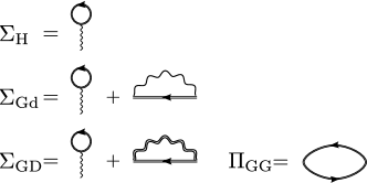
The Hartree approximation is the simplest approximation: the electron self-energy is approximated with the Hartree diagram, which can be written as

$$\Sigma_{\mathrm{H}}[G]^{M}_{ij}(\tau) =\imath\delta(\tau)\sum_{K}M_{ij}^{K}\phi^{M}_{K}\,,$$

and the phonon self-energy is neglected. The Hartree approximation is a time-local, static approximation which corresponds to a mean-field description.

The second approximation is the partially self-consistent Born approximation. This approximation also takes into account the Fock (F) diagram

$$\Sigma_{\mathrm{F}}[G,D]^{M}_{ij}(\tau) =\imath\sum_{kl,PQ}M_{ik}^{P}M_{lj}^{Q}D^{M}_{PQ}(\tau)G^{M}_{kl}(\tau)\,,$$

which is a time-nonlocal memory term describing single-phonon absorption/emission processes. The electron self-energy is given in this approximation by

$$\Sigma_{\mathrm{Gd}}[G]^{M}_{ij}(\tau) \equiv\Sigma_{\mathrm{H}}[G]^{M}_{ij}(\tau)+\Sigma_{\mathrm{F}}[G,d]^{M}_{ij}(\tau)\,,$$

where $d$ is the bare phonon propagator which means that the phonon self-energy is taken to be zero.

The third, and last, approximation is the fully self-consistent Born approximation in which the electron self-energy is given by

$$\Sigma_{\mathrm{GD}}[G,D]^{M}_{ij}(\tau) \equiv\Sigma_{\mathrm{H}}[G]^{M}_{ij}(\tau)+\Sigma_{\mathrm{F}}[G,D]^{M}_{ij}(\tau)\,,$$

and the phonon self-energy is approximated with the bubble diagram

$$\Pi_{\mathrm{GG}}[G]^{M}_{IJ}(\tau) =-\imath\sum_{kl,pq}M_{kl}^{I}M_{pq}^{J}G^{M}_{kq}(\tau)G^{M}_{pl}(-\tau)\,,$$ (4)

which describes simple phonon induced electron-hole excitation processes.

II.4 Observables

The electron and phonon propagators allow us to evaluate one-body observables, and additionally some more complicated observables such as the interaction energies. In the following, we introduce the observables considered in this work, and explain how they can be evaluated from the knowledge of the electron and phonon propagators.

The equilibrium electron one-body reduced density matrices are given by

$$\gamma_{ij} =\langle\hat{c}^{\dagger}_{j}\hat{c}_{i}\rangle$$

$$=-\imath G^{M}_{ij}(0^{-})\,,$$

where the angular brackets denote the grand-canonical ensemble average similar to Eq. (2). The diagonal elements of this density matrix give the electron density

$$n_{i} \equiv\gamma_{ii}\,,$$

while also off-diagonal elements are needed in order to evaluate electronic natural occupation numbers and/or orbitals. In order to address energetics, we consider the electron $E_{e}$, phonon $E_{p}$, and electron-phonon $E_{ep}$ interaction energies which are evaluated according to

$$E_{e} =\sum_{ij}h_{ij}\gamma_{ji}\,,$$

$$E_{pC} \equiv\sum_{IJ}\Omega_{IJ}\phi^{M}_{J}\phi^{M}_{I}\,,$$

$$E_{p} =E_{pC}+\imath\sum_{IJ}\Omega_{IJ}D^{M}_{JI}(0^{-})\,,$$

$$E_{epC} \equiv-\imath\sum_{Ijk}\phi_{I}^{M}M^{I}_{jk}G^{M}_{kj}(0^{-})\,,$$

$$E_{ep} =E_{epC}-\sum_{ij}\int\limits_{0}^{\beta}\!d\tau\;\big{(}\Sigma^{M}_{ij}(-\tau)-\Sigma^{M}_{H;ij}(-\tau)\big{)}G^{M}_{ji}(\tau)\,,$$

where the additional subscript $C$ refers to the classical (mean-field) piece of this energy. The total energy is then evaluated by summing all contributions according to

$$E\equiv E_{e}+E_{p}+E_{ep}\,.$$

This is in agreement with the energy functional

$$E_{\mathrm{GM}} =\imath\sum_{i}\partial_{\tau}G^{M}_{ii}(\tau)\big{|}_{\tau=0^{-}}$$

$$-\frac{1}{\imath}\sum_{IJ}\Omega_{IJ}\big{(}D_{JI}^{M}(0^{-})-\imath\phi_{J}^{M}\phi_{I}^{M}\big{)}\,,$$

which is known, in the purely electronic case, as the Galitski-Migdal functional. The derivation of this functional is given in the appendix A.

III Model

Our model system is a two-site Holstein model Schmidt and Schreiber (1987); Feinberg et al. (1990); Ranninger and Thibblin (1992); Alexandrov et al. (1994); Marsiglio (1995); de Mello and Ranninger (1997); Crljen (1998); Rongsheng et al. (2002); Qing-Bao and Qing-Hu (2005); Paganelli and Ciuchi (2008); Paganelli and Cuichi (2008); Firsov and Kudinov (1997); Chatterjee and Das (2000) which can be viewed as a minimal representation of a system in which electrons move between two molecules, so that they are coupled to the vibrational modes of these molecules. The Hamiltonian operator for a single primary vibrational mode of two identical molecules, henceforth referred to as sites 1 and 2, and minimal, localized basis for electrons is given by

$$\hat{H} =\omega_{0}\sum_{i=1}^{2}\hat{a}_{i}^{\dagger}\hat{a}_{i}-g\sum_{i=1}^{2}(\hat{a}^{\dagger}_{i}+\hat{a}_{i})\hat{n}_{i}+\hat{H}_{e}\,,$$

$$\hat{H}_{e} =-T\sum_{\sigma}\left(\hat{c}_{1\sigma}^{\dagger}\hat{c}_{2\sigma}+\hat{c}_{2\sigma}^{\dagger}\hat{c}_{1\sigma}\right)$$

where $\hat{a}_{i}$ is the phonon annihilation operator at site $i$, $\hat{c}_{i\sigma}$ is the electronic operator that annihilates an electron of spin $\sigma$ at site $i$, and $\hat{n}_{i}=\sum_{\sigma}\hat{c}^{\dagger}_{i\sigma}\hat{c}_{i\sigma}$ is the electron density operator at site $i$. The parameters $\omega_{0}$, $T$ and $g$ characterize the bare vibrational frequency, inter-site hopping and local electron-phonon interaction strength, respectively. The displacement and momentum operators, defined in this model as $\hat{u}_{i}\equiv\hat{\phi}_{1,i}$ and $\hat{p}_{i}\equiv\hat{\phi}_{2,i}$, allow us to rewrite the Hamiltonian operator as

$$\hat{H}= \frac{\omega_{0}}{2}\sum_{i=1}^{2}\big{(}\hat{p}_{i}^{2}+\hat{u}_{i}^{2}-1\big{)}-\sqrt{2}g\sum_{i=1}^{2}\hat{u}_{i}\hat{n}_{i}+H_{e}\,,$$

which is equivalent to the Hamiltonian of Eq. (II.1) with the matrix elements $\Omega_{i\varsigma_{i},j\varsigma_{j}}=\omega_{0}\delta_{ij}(\delta_{\varsigma_{i}\varsigma_{j}}-\sigma_{2;\varsigma_{i}\varsigma_{j}})/2$ and $M_{j\sigma,k\sigma^{\prime}}^{i\varsigma_{i}}=-\sqrt{2}g\delta_{\varsigma_{i},1}\delta_{\sigma\sigma^{\prime}}\delta_{ij}\delta_{jk}$. The properties of this model depend on two parameters, the adiabatic ratio

$$\gamma\equiv\frac{\omega_{0}}{T}\,,$$

and the effective interaction

$$\lambda \equiv\frac{2g^{2}}{T\omega_{0}} \,.$$ (5)

The adiabatic ratio $\gamma$ describes the relative energy scale of electrons and nuclei, while the effective interaction $\lambda$ is a measure of the coupling between the motions of these two constituents. This interaction is equal to the ratio of the Lang-Firsov Lang and Firsov (1962) bipolaron energy to the energy of two free electrons, and turns out to be an useful quantity for analyzing the many-body approximations.

IV Results

IV.1 Exact Properties

The main feature of the Holstein model is that it undergoes a cross-over, as a function of the interaction strength, from nearly free electrons to self-trapped quasi-particles known as polarons Fehske and Trugman (2007); Devreese and Alexandrov (2009). Our focus is in the two-electron case in which a phonon-mediated attractive interaction leads to the formation of a polaron pair referred to as a bipolaron. The purpose of this section is to clarify what is this correlated state and how it behaves as a function of the adiabatic ratio and effective interaction.

Our discussion starts with a limiting case obtained by rewriting the Hamiltonian operator as

$$\hat{H}= \omega_{0}\sum_{i=1}^{2}\bigg{(}\hat{a}_{i}^{\dagger}-\frac{g}{\omega_{0}}\hat{n}_{i}\bigg{)}\bigg{(}\hat{a}_{i}-\frac{g}{\omega_{0}}\hat{n}_{i}\bigg{)}$$

$$-\frac{g^{2}}{\omega_{0}}\sum_{i=1}^{2}\sum_{\sigma}\hat{c}^{\dagger}_{i\sigma}\hat{c}_{i\sigma}-\frac{2g^{2}}{\omega_{0}}\sum_{i=1}^{2}\hat{n}_{i\uparrow}\hat{n}_{i\downarrow}+\hat{H}_{e}$$

and considering the situation $2g^{2}/\omega_{0}\gg T$, namely $\lambda\gg 1$. The electron Hamiltonian $\hat{H}_{e}$ has the energy scale $T$ and is thus a candidate for a perturbation expansion, assuming that a finite converge radius exists. The unperturbed Hamiltonian obtained by setting $T$ to zero is diagonal in the electron and phonon site representations. The first term in this operator describes two shifted harmonic oscillators whose shift depends on the electron population and interaction strength. The second term is an electronic one-body term, and the last term represents an attractive interaction between electrons. The eigenstates can be labeled with eigenvalues $n_{i}$ of the site density operators $\hat{n}_{i}$ since they commute with the Hamiltonian. Then the degenerate two-electron ground state of the unperturbed system obtained by choosing $n_{1}=2,~{}n_{2}=0$ or $n_{2}=2,~{}n_{1}=0$ consists of a localized electron pair accompanied by a lattice distortion described by a shifted oscillator. This state is to be understood in this case as a bipolaron, that is a bound state of two electrons and a lattice displacement.

At finite hopping $T$, the electronic Hamiltonian $\hat{H}_{e}$ removes the degeneracy, and the competition between the de-localizing effect of the kinetic energy and the localizing effect of the interaction determines whether or not the ground state can be characterized with this quasi-particle. As we will soon see, in this case, the notion of a bipolaron is not perfect as there is no sharp distinction between a nearly-free electron and a bipolaronic state. In the following, we consider this regime and give a more precise definition of a bipolaron. This discussion requires some preliminaries starting with the transformation

$$\hat{a} \equiv(\hat{a}_{1}-\hat{a}_{2})/\sqrt{2}\,,$$

$$\hat{A} \equiv(\hat{a}_{1}+\hat{a}_{2})/\sqrt{2}\,,$$

where operators $\hat{a}$ and $\hat{A}$ fulfill the fundamental commutation relations for bosons. The original Hamiltonian can then be separated into two parts, $\hat{H}=\hat{H}_{tot}+\hat{H}_{rel}$, describing the total and relative motion of the dimer respectively. In particular,

$$\hat{H}_{tot} \equiv\omega_{0}\hat{A}^{\dagger}\hat{A}-g\hat{N}\hat{U}\,,$$ (6)

$$\hat{U} \equiv(\hat{A}+\hat{A}^{\dagger})/\sqrt{2}\,,$$ (7)

where $\hat{U}$ is the operator for the total displacement. This Hamiltonian simply corresponds to a shifted harmonic oscillator which can be solved exactly. The relative part of the Hamiltonian is given by

$$\hat{H}_{rel} \equiv\omega_{0}\hat{a}^{\dagger}\hat{a}-g(\hat{n}_{1}-\hat{n}_{2})\hat{u}+\hat{H}_{e}$$ (8)

$$\hat{u} \equiv(\hat{a}+\hat{a}^{\dagger})/\sqrt{2}\,,$$ (9)

where $\hat{u}$ is the operator for the relative displacement. The eigenvalue equation for the full Hamiltonian $\hat{H}$ can be written as

$$\hat{H}\ket{\Phi^{N}_{(n,j)}} =E^{N}_{(n,j)}\ket{\Phi^{N}_{(n,j)}}\,,$$

where we denote the $N$-electron eigenstates as $\ket{\Phi^{N}_{(n,j)}}$ and their energies as $E^{N}_{(n,j)}$. The double labeling $(n,j)$ reflects the fact that, because of the partitioning of $\hat{H}$ into two parts, the full eigenstates can be written as the products

$$\ket{\Phi^{N}_{(n,j)}} =\ket{n,N}\ket{\Psi^{N}_{j}}\,,$$

$$\hat{H}_{tot}\ket{n,N} =\left(\omega_{0}n-\frac{g^{2}N^{2}}{2\omega_{0}}\right)\ket{n,N}\,,$$

$$\hat{H}_{rel}\ket{\Psi^{N}_{j}} =\varepsilon_{n}^{N}\ket{\Psi^{N}_{j}}\,,$$

where $\ket{n,N}$ and $\ket{\Psi^{N}_{j}}$ are the eigenstates of $\hat{H}_{tot}$ and $\hat{H}_{rel}$ respectively. The Hamiltonian commutes with the total spin $\hat{S}^{2}$ and z component $\hat{S}_{z}$, $[\hat{S}^{2},\hat{H}]=0$ and $[\hat{S}_{z},\hat{H}]=0$, therefore we can classify states according to their spin angular momentum. The ground state for two electrons ($N=2$) is in the subspace with $S(S+1)=0$ and $S_{z}=0$. The relative Hamiltonian is also invariant under the operation of the parity operator, which swaps indices $1$ and $2$ and changes $\hat{u}$ to $-\hat{u}$. Hence the eigenstates of $\hat{H}_{rel}$ have either even or odd parity. In particular, the ground state is even under parity operation. Thus by symmetry, we have $\langle\hat{u}\rangle$=0, $\langle\hat{n}_{1}\rangle=\langle\hat{n}_{2}\rangle=1$, which are expectation values taken with respect to the symmetric ground state.

Figure 2: The top panel displays the two-electron $\varepsilon^{N=2}_{0}$, two times one-electron $2\varepsilon^{N=1}_{0}$ ground-state energies, and double occupancy $\langle\hat{n}_{1\uparrow}\hat{n}_{1\downarrow}\rangle$ as a function of electron-phonon interaction strength $\lambda$. The energies are represented on the right (Energy) and double-occupancies on the left (Probability) axis, respectively. The bottom panel shows the joint probabilities $P_{ij}(u)$ to find electrons at the sites $i,j$ and nuclei at the relative displacement $u$, and the probability $P(u)$ to find the nuclear displacement at $u$ for three different electron-phonon interaction strengths. The lowest BO surfaces $E_{0}$ for different cases are shown in the same panels. They are plotted according to Eq.(15a) with only a constant shift, in order to let their minima touch the bottom of the figures. Left: Small hopping regime, $\gamma=8$ in the anti-adiabatic limit. Right: Large hopping regime, $\gamma=1/8$ in the adiabatic limit. (color online)

The two-electron singlet Hilbert space is then spanned by

$$\ket{1}_{e} =\frac{1}{\sqrt{2}}\left(\hat{c}_{1\uparrow}^{\dagger}\hat{c}_{2\downarrow}^{\dagger}-\hat{c}_{1\downarrow}^{\dagger}\hat{c}_{2\uparrow}^{\dagger}\right)\ket{0}_{e}\,,$$

$$\ket{2}_{e} =\frac{1}{\sqrt{2}}\left(\hat{c}_{1\uparrow}^{\dagger}\hat{c}_{1\downarrow}^{\dagger}+\hat{c}_{2\uparrow}^{\dagger}\hat{c}_{2\downarrow}^{\dagger}\right)\ket{0}_{e}\,,$$ (10)

$$\ket{3}_{e} =\frac{1}{\sqrt{2}}\left(\hat{c}_{1\uparrow}^{\dagger}\hat{c}_{1\downarrow}^{\dagger}-\hat{c}_{2\uparrow}^{\dagger}\hat{c}_{2\downarrow}^{\dagger}\right)\ket{0}_{e}\,,$$

where $\ket{0}_{e}$ denotes the electronic vacuum. The relative Hamiltonian can be written in this subspace as the operator-valued matrix

$$\boldsymbol{\hat{H}}_{rel}^{N=2}=\begin{pmatrix}\omega_{0}\hat{a}^{\dagger}\hat{a}&-2T&0\\ -2T&\omega_{0}\hat{a}^{\dagger}\hat{a}&-2g\hat{u}\\ 0&-2g\hat{u}&\omega_{0}\hat{a}^{\dagger}\hat{a}\end{pmatrix}\,.$$ (11)

This Hamiltonian can be diagonalized numerically by expressing the phonon operators as matrices in a basis set of Fock number states $\left\{\ket{n}_{ph}\right\}$, which in practical calculations is truncated up to a maximum value $N_{ph}$, i.e. $n\leq N_{ph}$. In our exact diagonalization approach $N_{ph}=100$ turns out to be sufficient for the convergence of the relevant quantities. Alternatively, using the fact that

$$\hat{a}^{\dagger}\hat{a} =\frac{\hat{p}^{2}}{2}+\frac{\hat{u}^{2}}{2}-\frac{1}{2}\,,$$ (12)

and by choosing a finite difference representation for momentum $\hat{p}$ and the displacement $\hat{u}$ operators, the diagonalization can also be performed in real space. Either of the two diagonalization approaches yield accurate ground-state energies as long as the truncated basis for nuclear motion is large enough. However, each approach has its own advantages in calculating certain properties.

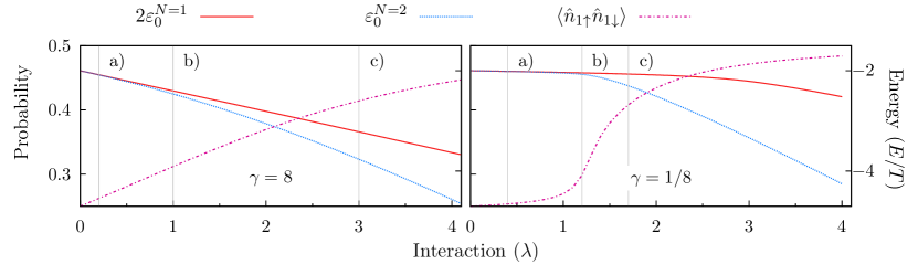
We are now set to investigate the finite $T$ properties of this model and illustrate the bipolaronic nature of the system. In Fig. 2, we show results for two sets of parameters, corresponding to the small and large electron hopping regimes: $\gamma=8$ in anti-adiabatic regime on the left hand side and $\gamma=1/8$ in adiabatic regime on the right hand side. The top panels show the two-electron ground-state energies $\varepsilon_{0}^{N=2}$, that is the lowest eigenvalues of $\boldsymbol{\hat{H}}_{rel}^{N=2}$, as a function of the effective electron-phonon interaction $\lambda$ for both adiabatic ratios $\gamma$. These ground-state energies are compared with two times the one-electron ground-state energies $2\varepsilon_{0}^{N=1}$, which are obtained by diagonalizing the relative Hamiltonian represented in the one-electron subspace with $S_{z}=1/2$ (same as $S_{z}=-1/2$). The figure shows that when the electron phonon interaction strength is small, the energies are very close to one another, and when the electron-phonon interaction strength is increased, the two-electron ground-state becomes much lower in energy and decreases faster as a function of the interaction. This suggests a physical picture in which for weak interactions the two electrons, or polarons, are almost independent. A strong electron-phonon interaction, on the other hand, gives rise to a large effective attraction between electrons leading to a strongly bound electron, or polaron pair, which is seen as increased binding energy $2\varepsilon_{0}^{N=1}-\varepsilon_{0}^{N=2}$. This picture can be elucidated by investigating the double occupancy which is a correlation function of the occupations of spin up and down electron at the same site. Without loss of generality, we focus on site 1 for the double occupancy

$$\langle\hat{n}_{1\uparrow}\hat{n}_{1\downarrow}\rangle =\bra{\Psi_{0}^{2}}\hat{n}_{1\uparrow}\hat{n}_{1\downarrow}\ket{\Psi_{0}^{2}},$$

where $\hat{n}_{1\alpha}=\hat{c}_{1\alpha}^{\dagger}\hat{c}_{1\alpha}$, and $\ket{\Psi_{0}^{2}}$ is the two-electron ground state. The double-occupancy is shown in the top panels of Fig. 2 as a function of the electron phonon interaction strength $\lambda$ for both adiabatic ratios $\gamma$. The figure shows that this quantity is equal to one-quarter for a non-interacting system stating due to symmetry that it is equally probable to find electrons in the same of different sites. As the interaction is increased, the double-occupancy approaches one-half irrespectively of the adiabatic ratio. This result implies that an electron-pair is formed as a function of the interaction. The effect of the adiabatic ratio is that the crossover from the non-interacting system to a system in which an electron pair is formed happens more abruptly in the adiabatic $\gamma=1/8$ case.

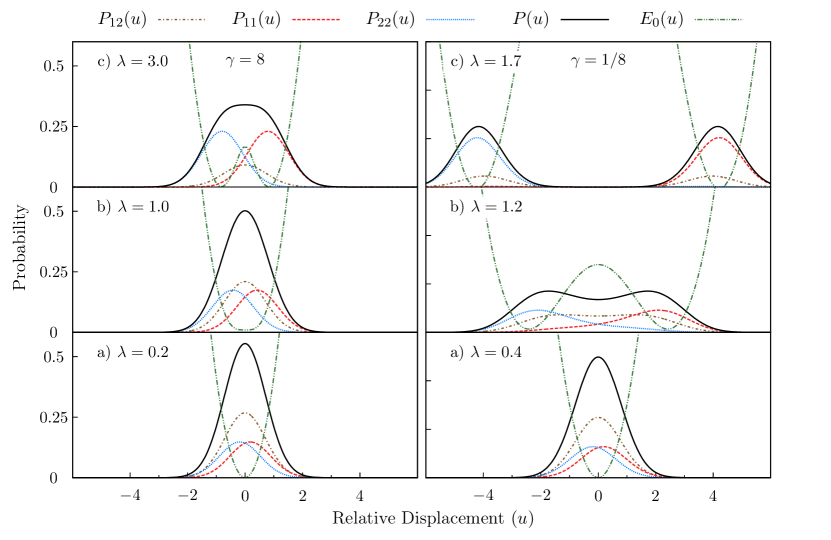
The increase of the binding energy indicates a crossover to a strongly bound two-electron state when the interaction is strong enough. This goes hand in hand with an increase of the double-occupancy which says that the probability of finding two electrons at the same site is large compared to the probability of finding them at different sites. This picture can be made more quantitative by introducing the joint probability of finding electrons at the sites $i,j$ and nuclei at the relative coordinate $u$. The joint probability is defined as

$$P_{ii}(u) \equiv\lvert\langle i\uparrow,i\downarrow;u|\Psi_{0}^{2}\rangle\rvert^{2}\,,$$

$$P_{ij}(u) \equiv\sum_{\begin{subarray}{c}\sigma\sigma^{\prime}\\ \sigma\neq\sigma^{\prime}\end{subarray}}\lvert\langle i\sigma,j\sigma^{\prime};u|\Psi_{0}^{2}\rangle\rvert^{2}\,,i\neq j\,,$$ (13)

where $\lvert i\sigma,j\sigma^{\prime};u\rangle\equiv\hat{c}^{\dagger}_{i\sigma}\hat{c}^{\dagger}_{j\sigma^{\prime}}\lvert 0\rangle_{e}\lvert u\rangle$ with $\lvert u\rangle$ being an eigenstate of $\hat{u}$. The lower panels a), b) and c) of Fig. 2 display these probabilities. The probability of finding electrons on the same site is in the non-interacting limit equal to the probability of finding them at different sites. As the electron-phonon interaction is increased, the maximum of the joint probability of finding electrons on the site one (two) increases and the position of the maximum moves towards larger (smaller) values of the relative displacement. On the other hand, the maximum of the joint probability of finding electrons on neighboring sites decreases and the position of this maximum remains fixed at the origin as the interaction is increased. Thus for any non-zero interaction it is more likely to find the electrons occupying the same site and accompanied by a non-zero displacement. This however does not mean that the ground state is characterized well by the notion of an electron pair and an associated displacement. This leads us to the concept of a working definition of a bipolaron. We regard for the present work a bipolaron being a good representative of the ground state when the maxima of the joint probabilities of electrons appearing at the same site, $\max_{u}P_{ii}(u),i=1,2$, cf. Eq. (13), is at least two times larger than the joint probability to finding the electrons at different sites $\max_{u}P_{12}(u)$. We note that this definition is not unique, and depending on ones viewpoint other choices can be made, but it does denote a situation in which an electron pair accompanied by a displacement is a dominant feature of the ground state. This working definition allows us to summarize the results of Fig. 2 by saying that panels a) and c) represent in both adiabatic and anti-adiabatic regimes two nearly-free electrons and a bipolaron, respectively. The middle panel b), on the other hand, corresponds to a ground state which is not characterized well by a single notion of either two nearly-free electrons, two polarons, or a bipolaron.

The lower panels of Fig. 2 also display the probability

$$P(u)\equiv\sum_{i}P_{ii}(u)+P_{12}(u)$$ (14)

of finding the nuclei at relative coordinate $u$. The figure shows that prior to the bipolaron formation, this probability distribution has a single maximum located at the origin. As the interaction is increased, the ground state becomes more and more bipolaron-like and the nuclear distribution $P(u)$ starts to split symmetrically, as it should due to the symmetry of the Hamiltonian. In the adiabatic case, it already forms two well-separated peaks when $\lambda=1.7$ in panel c), indicating that it is more likely to find the nuclei at $u$ far from zero, either positive or negative. In the anti-adiabatic case, this splitting happens much slower as a function of $\lambda$ and the peaks are still not well-separated at $\lambda=3$. However, we already see the trend of the splitting behavior which is the same as in the adiabatic case, the only difference is that a quantitatively much larger $\lambda$ is needed to split the nuclear distribution. Hence, the formation of the bipolaron coincides with the splitting of the nuclear distribution in the adiabatic limit, while in the anti-adiabatic case, the bipolaron formation does not necessarily imply the splitting $P(u)$, and there is a smaller nuclear displacement associated with the bipolaron compared to the displacement in the adiabatic case.

As a last topic on exact properties, we discuss the adiabatic limit which leads us naturally to the Born-Oppenheimer (BO) approximation. This perspective leads us to scrutinize the splitting of the nuclear probability $P(u)$ using the adiabatic potential energy surfaces. We use Eq. (12), and set $\hat{p}\equiv 0$ in the BO approximation. Then we diagonalize the 3 by 3 block in Eq. (11), where $u$ is now taking the role of a parameter. The eigenvalues $E_{0}(u)$, $E_{1}(u)$, and $E_{2}(u)$ correspond to the ground-state, first, and second excited-state BO surfaces (Fig. 2) respectively

$$E_{0}(u) =\omega_{0}\left(\frac{u^{2}}{2}-\frac{2}{\gamma}\sqrt{1+\frac{\lambda\gamma}{2}u^{2}}\right)\,,$$ (15a)

$$E_{1}(u) =\frac{u^{2}}{2}\omega_{0}\,,$$ (15b)

$$E_{2}(u) =\omega_{0}\left(\frac{u^{2}}{2}+\frac{2}{\gamma}\sqrt{1+\frac{\lambda\gamma}{2}u^{2}}\right).$$ (15c)

In the BO or adiabatic approximation the nuclei are moving on the ground-state surface $E_{0}(u)$, which behaves as an effective potential. The shape of this potential determines therefore to a large extent the shape of $P(u)$. From the figure, we clearly see that the formation of a double minimum in $E_{0}(u)$ directly attributes to the splitting of $P(u)$. In particular, in the adiabatic regime $\gamma=1/8$, this correspondence is a very good approximation because the kinetic energy of the electrons is much larger than the phonon frequency, and hence the ground-state BO surface is enough to capture the motion of the nuclei. In Eq. (15a), we notice that the second term in the parenthesis, which is just the energy difference between the ground and the first excited BO surfaces (Eq. (15b)), is small when $\gamma$ is large (anti-adiabatic). Hence in the anti-adiabatic regime, the coupling between the lowest two surfaces is large, especially near the origin $u=0$. This is why in Fig. 2 b) on the left, the correspondence between the potential surface and the shape of the probability distribution is not convincible. The reason is that the first excited surface also influences the nuclear motion and considering only the ground BO surface is not enough.

From Eq. (15a) it can also be worked out that the condition for the formation of a double minimum, at $u_{1,2}=\pm\sqrt{2(\lambda^{2}-1)/\lambda\gamma}$, is for $\lambda>1$ simply given by taking the derivative of $E_{0}(u)$ with respect to $u$. We can write down the ground-electronic state $\ket{\chi_{0}^{BO}(u)}$ in the BO approximation in terms of the basis defined in Eq. (10)

$$\ket{\chi_{0}^{BO}(u)}=\frac{\ket{1}_{e}+\sqrt{1+\frac{\lambda\gamma}{2}u^{2}}\ket{2}_{e}+\sqrt{\frac{\lambda\gamma}{2}}u\ket{3}_{e}}{(2+\lambda\gamma u^{2})^{1/2}}.$$

Using this state, we can compute the double occupancy at site $1$ in the BO approximation

$$\langle\hat{n}_{1\uparrow}\hat{n}_{1\downarrow}\rangle =\int_{-\infty}^{\infty}\mathrm{d}uP_{BO}(u)\bra{\chi_{0}^{BO}(u)}\hat{n}_{1\uparrow}\hat{n}_{1\downarrow}\ket{\chi_{0}^{BO}(u)}$$

$$=\int_{-\infty}^{\infty}\mathrm{d}uP_{BO}(u)\frac{1+\lambda\gamma u^{2}+2\sqrt{\frac{\lambda\gamma}{2}}\sqrt{1+\frac{\lambda\gamma}{2}u^{2}}u}{2(2+\lambda\gamma u^{2})}$$

$$=\int_{-\infty}^{\infty}\mathrm{d}uP_{BO}(u)\frac{1+\lambda\gamma u^{2}}{2(2+\lambda\gamma u^{2})},$$

where $P_{BO}(u)$ is the nuclear distribution $P(u)$ in the BO picture. We have used the fact the BO state is factorizable and $P_{BO}(u)$ is an even function of $u$. Next, we consider the case when $\gamma\rightarrow 0$. If $\lambda<1$, $E_{0}$ reaches its minimum at 0. We perform the harmonic approximation by calculating

$$\frac{1}{\omega_{0}}\frac{d^{2}E_{0}}{du^{2}}\bigg{|}_{0}=1-\lambda,$$

which means $P_{BO}(u)$ is peaked at the origin with width $\sim(1-\lambda)^{-1/4}$, independent of $\gamma$. For $\lambda>1$ the barrier between the double minimum at $u_{1,2}$ becomes infinite. Hence, we can consider each well separately and perform the harmonic approximation around $u_{1,2}$. By taking the second derivative of $E_{0}(u)$ with respect to $u$ and evaluating it at the two minima $u_{1,2}$, we obtain

$$\frac{1}{\omega_{0}}\frac{d^{2}E_{0}}{du^{2}}\bigg{|}_{u_{1,2}}=\frac{\lambda^{2}-1}{\lambda^{2}}.$$

Thus for $\lambda>1$, $P_{BO}$ can be approximated by two Gaussian wave packets around the positions $u_{1,2}$ with width $\sim\left[\lambda^{2}/(\lambda^{2}-1)\right]^{1/4}$, independent of $\gamma$. Moreover, in the limit $\gamma\rightarrow 0$, the second term in the integrand changes very slowly near $u_{max}$, either $0$ or $u_{1,2}$, at which $P_{BO}$ is peaked. This is due to the fact that the rate of change is proportional to $\sqrt{\gamma}\rightarrow 0$. Hence we can replace the term $\lambda\gamma u^{2}$ by $\lambda\gamma u_{max}^{2}$, for either $\lambda<1$ or $\lambda>1$, namely

$$\langle\hat{n}_{1\uparrow}\hat{n}_{1\downarrow}\rangle \simeq\frac{1+\lambda\gamma u_{max}^{2}}{2(2+\lambda\gamma u_{max}^{2})}\int_{-\infty}^{\infty}\mathrm{d}uP_{BO}(u)$$

$$=\begin{cases}1/4&\lambda<1\\ \frac{2\lambda^{2}-1}{4\lambda^{2}}&\lambda>1.\end{cases}$$

This demonstrates the sharp change, a kink at $\lambda=1$, of the double occupancy for an increasing electron-phonon interaction in the adiabatic case, and its value is always between $1/4$ and $1/2$. As a final remark, we emphasize that the appearance of the double-well structure for $\lambda>1$ in the BO picture is closely related to the issue of symmetry-breaking discussed in the following sections.

IV.2 Mean-Field

Let us begin scrutinizing the Holstein dimer from the perspective of our many-body approximations by considering the simplest self-consistent method, the Hartree approximation. This self-energy approximation gives rise to a mean-field approximation in which the electrons feel the nuclear displacement instantaneously. The displacement expectation value

$$u_{i} =\sqrt{2}gn_{i}/\omega_{0}\,,$$

allows us to write the Hartree self-energy as

$$\Sigma_{\mathrm{H};ij}^{M}(\tau) =-\imath\delta_{ij}\delta(\tau)T\lambda n_{i}\,,$$ (16)

where $n_{i}$ is the spin-summed site density. This term is time-local which means that it can be accounted for with an effective one-body Hamiltonian given by

$$\boldsymbol{h}_{\mathrm{H}}^{M}\equiv\begin{pmatrix}-T\lambda n_{1}-\mu&-T\\ -T&-T\lambda n_{2}-\mu\end{pmatrix}\,,$$ (17)

where $\mu$ is the chemical potential which is to be chosen in the following. We refer to the nonlinear eigenvalue equations associated with this matrix as the Hartree equations. The two eigenvalues and eigenvectors of these equations are given by

$$\epsilon_{\mathrm{H},\pm} =-\frac{T\lambda N}{2}\pm T\sqrt{1+\lambda^{2}(n_{1}-N/2)^{2}}-\mu\,,$$

$$\psi_{\mathrm{H};1,\pm} =\frac{-1}{\sqrt{1+(\lambda n_{1}+\mu/T+\epsilon_{\mathrm{H},\pm}(n_{1})/T)^{2}}}\,,$$

$$\psi_{\mathrm{H};2,\pm} =\frac{\lambda n_{1}+\mu/T+\epsilon_{\mathrm{H},\pm}(n_{1})/T}{\sqrt{1+(\lambda n_{1}+\mu/T+\epsilon_{\mathrm{H},\pm}(n_{1})/T)^{2}}}\,,$$

where $N$ is the electron number and $\lambda$ the dimensionless interaction of Eq. (5). The eigendecomposition can be used to form a self-consistency relation for the density $n_{1}$ at the first site. This relation can be written for two electrons ($N=2$) by fixing the chemical potential at

$$\mu =-T\lambda\,,$$ (18)

and taking the zero-temperature limit ($\beta\gg 2T)$ so that it is given by

$$n_{1} =2|\psi_{\mathrm{H};1,-}|^{2}$$

$$=\frac{2}{1+\big{(}\lambda(n_{1}-1)-\sqrt{1+\lambda^{2}(n_{1}-1)^{2}}\big{)}^{2}}\,.$$

By reordering terms this can be written as a cubic equation for the spin-summed site density at site $1$, which has the three solutions

$$n_{s} \equiv 1\,,$$

$$n_{a\pm} \equiv 1\pm\sqrt{1-1/\lambda^{2}}\,,$$

where subscript $s$ and $a$ stand for symmetric and asymmetric, respectively. The symmetric solution ($n_{s}$) is always real valued and hence an acceptable candidate for the lowest energy solution. The asymmetric solutions ($n_{a\pm}$) are however complex when $\lambda<1$ and therefore acceptable solutions only when they become real valued, that is for $\lambda\geq 1$. This means that at the critical interaction $\lambda_{C}^{\mathrm{H}}\equiv 1$ a single physically acceptable solution splits into three acceptable solutions. Our next task is then to check which one is the lowest energy solution. This can be achieved by using the spin-summed reduced density matrices

$$\gamma_{s} \equiv\begin{pmatrix}1&1\\ 1&1\end{pmatrix}\,,$$

$$\gamma_{a\pm} \equiv\begin{pmatrix}n_{a\pm}&1/\lambda\\ 1/\lambda&2-n_{a\pm}\end{pmatrix}$$

where the asymmetric density matrix is only defined for $\lambda\geq 1$. These density matrices together with the displacement expectation value, and momentum expectation value ($p_{i}=0$) can be used to evaluate the electron $E_{e}$, phonon $E_{p}$, and electron-phonon $E_{ep}$ interaction energies. The energy components of the symmetric solution are given

$$E_{e,s}/T =-2\,,$$

$$E_{p,s}/T =\lambda\,,$$

$$E_{ep,s}/T =-2\lambda\,,$$

and those of the asymmetric solution by

$$E_{e,a\pm}/T =-2/\lambda\,,$$

$$E_{p,a\pm}/T =2\lambda-1/\lambda\,,$$

$$E_{ep,a\pm}/T =-4\lambda+2/\lambda\,.$$

These different energy components allow us to evaluate the total energies

$$E_{s}/T =-\lambda-2\,,$$ (19)

$$E_{a\pm}/T =-2\lambda-1/\lambda\,,$$ (20)

which indicate that the asymmetric solution is the lowest energy solution which by definition is the ground state.

As discussed in Sec. IV.1, for the ground state of the exact solution, the double-occupancy on a given site approaches one-half for large interactions ($\lambda$) representing a bipolaron state. On the other hand, in the mean-field approach, we have found that above the critical interaction $\lambda_{C}^{\mathrm{H}}$, the ground state becomes degenerate with two symmetry-broken states. In these states the electrons prefer to populate the same site, and as the displacement is linearly proportional to the electron density at that site, this electron pair is accompanied by a lattice deformation. This supports the conclusion that the mean-field approach mimics the formation of a bipolaron by symmetry-breaking and localization. The formation appears continuously, although in contrast to the exact case not smoothly, and very rapidly, in the manner of a bifurcation.

IV.3 Beyond Mean-Field, Asymptotic Solution

Symmetry-breaking is a well-known feature of mean-field theories Helgaker et al. (2000); Reimann and Manninen (2002); Ivanov (2002). This leads us to question what is needed to remedy this situation. Let us explore this thought by scrutinizing the partially self-consistent Born approximation. Although we are not in a position to be able to handle this approximation purely analytically, we can investigate its asymptotic behavior in the adiabatic and anti-adiabatic limits.

The self-energy is a sum of the Hartree and Fock self-energies. The former is given in Eq. (16) and the latter can be written as

$$\Sigma_{\mathrm{F}}[G]^{M}_{ij}(\tau) =\imath\omega_{0}T\lambda\delta_{ij}d(\tau)G^{M}_{ii}(\tau)\,,$$

where we introduced

$$2\imath d(\tau) =\theta(\tau)\big{[}f_{-}(\beta\omega_{0})e^{\omega_{0}\tau}+\big{(}1+f_{-}(\beta\omega_{0})\big{)}e^{-\omega_{0}\tau}\big{]}$$

$$+\theta(-\tau)\big{[}f_{-}(\beta\omega_{0})e^{-\omega_{0}\tau}+\big{(}1+f_{-}(\beta\omega_{0})\big{)}e^{\omega_{0}\tau}\big{]}\,.$$

as the diagonal elements of the displacement-displacement component of the bare phonon propagator.

Let us start with the adiabatic limit in which $\omega_{0}\ll T$ independent of $\lambda$. In this limit, the electron propagator decays much faster than the phonon propagator allowing us to approximate the latter with a constant value. The $\omega_{0}\rightarrow 0$ limit gives the constant

$$\imath\omega_{0}d(\tau) \rightarrow\frac{1}{\beta}\,,$$

which can be used to write the self-energy in the imaginary-frequency representation as

$$\Sigma_{\mathrm{Gd}}[G]^{M}_{ij}(p_{n}) =\Sigma_{\mathrm{H}}[G]^{M}_{ij}+\delta_{ij}\frac{T\lambda}{\beta}G^{M}_{ii}(p_{n})\,,$$

where $p_{n}=\imath\pi(2n+1)/\beta$ is a fermionic imaginary frequency. The electron propagator then satisfies the Dyson equation

$$\boldsymbol{G}^{M}(p_{n}) =\boldsymbol{g}^{M}(p_{n})+\boldsymbol{g}^{M}(p_{n})\boldsymbol{\Sigma}_{\mathrm{Gd}}[G]^{M}(p_{n})\boldsymbol{G}^{M}(p_{n})$$

which is diagonal in the frequencies, and one can see that in the zero-temperature limit $\beta\gg 1$ the self-energy approaches the Hartree self-energy. This analysis suggests that the partially self-consistent Born approximation reduces to the mean-field approximation in the adiabatic limit, and is thus similarly expected to break the symmetry at $\lambda=1$.

The anti-adiabatic limit $\omega_{0}\gg T$, independent of $\lambda$, can be treated similarly. Now the phonon propagator decays rapidly compared to the electron propagator and is non-negligible only for $|\tau|\rightarrow 0$ or $\beta$. This allows us to approximate the phonon propagator with its value at the limit $\omega_{0}\rightarrow\infty$ which amounts to

$$\frac{\omega_{0}e^{\mp\omega_{0}\tau}}{1-e^{-\beta\omega_{0}}} \rightarrow\delta_{\pm}(\tau)\,,$$

where we introduced a delta function defined as $\delta_{\pm}(\tau)\equiv\delta(\tau^{\mp})$ on the intervals $[0,\beta]$ and $[-\beta,0]$, respectively, and zero otherwise. The phonon propagator can therefore be written as

$$2\imath\omega_{0}d(\tau) =\delta_{+}(\beta-\tau)+\delta_{+}(\tau)$$

$$+\delta_{-}(-\beta-\tau)+\delta_{-}(\tau)\,,$$

where $\tau\in[-\beta,\beta]$. This approximation enters the self-energy which in turn appears as an integral kernel in the convolution

$$\big{[}\boldsymbol{\Sigma}_{\mathrm{F}}^{M}\star\boldsymbol{G}^{M}\big{]}_{ij}(\tau) =-\imath\sum_{k}\int\limits_{0}^{\beta}\,d\tau^{\prime}\;\Sigma_{\mathrm{F}}[G]_{ik}^{M}(\tau-\tau^{\prime})G^{M}_{kj}(\tau^{\prime})$$

$$=-\imath\frac{T\lambda}{2}\big{(}G^{M}_{ii}(0^{+})+G^{M}_{ii}(0^{-})\big{)}G^{M}_{ij}(\tau),$$

where $\tau$ is restricted on the open interval $(0,\beta)$ since the values of this convolution are different at the end points. The convolution appears as an integral kernel in the Dyson equation which allows us to disregard the discontinuity at the end points. Then the identity $G_{ij}^{M}(0^{+})-G_{ij}^{M}(0^{-})=-\imath\delta_{ij}$ allows us to conclude that

$$\Sigma_{\mathrm{Gd}}[G]^{M}_{ij}(\tau)= \Sigma_{\mathrm{H}}[G]^{M}_{ij}$$

$$+\delta_{ij}\delta(\tau)T\lambda G^{M}_{ii}(0^{-})-\imath\delta_{ij}\delta(\tau)\frac{T\lambda}{2}$$

$$= \frac{\Sigma_{\mathrm{H}}[G]^{M}_{ij}}{2}+\imath\delta_{ij}\delta(\tau)\frac{\mu}{2}\,,$$

which shows that the self-energy reduces to the Hartree self-energy plus a constant contributing to the chemical potential. We conclude that in the anti-adiabatic limit, the partially self-consistent Born approximation becomes again identical to the mean-field but now with a renormalized interaction $\lambda/2$. This new interaction means that also the bifurcation point shifts to $\lambda=2$. We therefore expect that partial self-consistency does not prevent symmetry-breaking and that, unlike in the Hartree approximation, the bifurcation point is not independent of the adiabatic ratio.

IV.4 Beyond Mean-Field, Phonon Vacuum Instability

The discussion on the properties of the nuclear system has so far remained at a mean-field level. In the following we investigate how the phonon propagator is affected by the interaction. The phonon vacuum instability is a known issue when the propagator is dressed with a bare polarization bubble, that is one evaluated with non-interacting electron propagators Alexandrov et al. (1994); Alexandrov and Mott (1994). Next, we revise this peculiarity in the context of the Holstein dimer, and investigate what happens when we use a symmetry-broken instead of a symmetric electron propagator.

The phonon propagator satisfies in the imaginary-frequency representation the equation

$$\boldsymbol{D}^{M}(\nu_{n}) =\boldsymbol{d}^{M}(\nu_{n})+\boldsymbol{d}^{M}(\nu_{n})\boldsymbol{\Pi}[G]^{M}(\nu_{n})\boldsymbol{G}^{M}(\nu_{n}),$$

where $\nu_{n}=\imath 2\pi n/\beta$ is a bosonic imaginary-frequency. Observables are then accessible by either using analytic continuation to real frequencies, or by transforming back to imaginary-time and taking the limit $0^{-}$ to evaluate time-local observables. The Lehmann representation, or a partial fraction decomposition, of the phonon propagator convenient for either of the two choices can be accomplished by calculating the roots of the characteristic function

$$\det\big{(}\nu_{n}^{2}\boldsymbol{1}-\omega_{0}^{2}\boldsymbol{1}-\omega_{0}\boldsymbol{\mathsf{\Pi}}[G]^{M}(\nu_{n})\big{)}\,,$$

where $\boldsymbol{1}$ denotes the identity matrix, and $\mathsf{\Pi}[G]^{M}_{ij}(\nu_{n})\equiv\Pi[G]^{M}_{1i,1j}(\nu_{n})$ the displacement-displacement component of the phonon self-energy. The roots of this equation are usually understood via analytic continuation as the renormalized phonon frequencies.

The imaginary-frequency representation of the self-energy given in Eq. (4) can be written as

$$\mathsf{\Pi}[G]_{ij}^{M}(\nu_{n}) =\frac{2T\omega_{0}\lambda}{\beta}\sum_{q=-\infty}^{\infty}G_{ij}^{M}(p_{q})G_{ji}^{M}(p_{q}-\nu_{n})\,.$$

The electron propagator is approximated with the mean-field propagator

$$\boldsymbol{G}_{\mathrm{H}}^{M}(p_{n}) =\big{(}p_{n}\boldsymbol{1}-\boldsymbol{h}_{\mathrm{H}}^{M}\big{)}^{-1}\,,$$

where $\boldsymbol{h}_{\mathrm{H}}^{M}\equiv\boldsymbol{h}_{\mathrm{H}}^{M}(\lambda/\lambda_{C})$ is defined in Eq. (17), and the critical interaction $\lambda_{C}\geq 1$ has been introduced to be able to represent also the partially self-consistent propagator, which we have shown to reduce to the mean-field one but with a renormalized interaction. This approximation leads for a sufficiently low temperature $\beta\gg 2T$ to the self-energy

$$\mathsf{\Pi}[G_{\mathrm{H}}]_{ij}^{M}(\nu_{n}) =\frac{2T^{2}\omega_{0}\lambda\bar{\lambda}^{-1}}{\nu_{n}^{2}-4\bar{\lambda}^{2}T^{2}}\begin{pmatrix}1&-1\\ -1&1\end{pmatrix}\,,$$

where the effective interaction

$$\bar{\lambda}\equiv\bar{\lambda}(\lambda)=\theta(\lambda-\lambda_{C})\lambda/\lambda_{C}+\theta(\lambda_{C}-\lambda)$$

is introduced to allow us to incorporate both the symmetric ($\lambda<\lambda_{C}$) and asymmetric ($\lambda>\lambda_{C}$) cases in a single equation. The characteristic function is then evaluated with this self-energy and set to zero which leads to the two equations

$$0 =x^{2}-\omega_{0}^{2}\,,$$

$$0 =x^{2}-\omega_{0}^{2}-\frac{4T^{2}\omega_{0}^{2}\lambda\bar{\lambda}^{-1}}{x^{2}-4\bar{\lambda}^{2}T^{2}}\,,$$

where $x$ denotes the sought solution. The roots of the first equation are just the bare phonon frequencies $\omega_{0}$ which reflects the fact that the total displacement $U$ couples only to the electron number and therefore its frequency remains invariant. The second equation can be re-written as a fourth order polynomial equation whose roots $\omega_{\pm},-\omega_{\pm}$ satisfy

$$\frac{\omega_{\pm}^{2}}{T^{2}} =2\big{(}\gamma^{2}/4+\bar{\lambda}^{2}\big{)}\Bigg{(}1\pm\sqrt{1+\frac{\gamma^{2}\bar{\lambda}^{-1}(\lambda-\bar{\lambda}^{3})}{\bar{\lambda}\big{(}\gamma^{2}/4+\bar{\lambda}^{2}\big{)}^{2}}}\Bigg{)}\,.$$

These roots represent the renormalized phonon frequencies related to the relative displacement $u$. The important observation here is that these frequencies should be real valued, but in fact $\omega_{-}$ becomes imaginary when $\lambda-\bar{\lambda}^{3}>0$ which indicates the phonon vacuum instability. The critical value of interaction at which this happens is

$$\lambda>1$$

for a symmetric $\bar{\lambda}=1$ electron propagator, and

$$\lambda<\lambda_{C}^{3/2}$$

for an asymmetric $\bar{\lambda}=\lambda/\lambda_{C}$ electron propagator. This shows that there is a finite region $\lambda\in(1,\lambda_{C}^{3/2})$ in which imaginary phonon frequencies appear.

The imaginary frequencies have a direct impact on observables which are obtained, for example, using the displacement-displacement component $\mathsf{D}^{M}_{ij}(\nu_{n})\equiv D_{1i,1j}^{M}(\nu_{n})$ of the phonon propagator. This component can be written as

$$\boldsymbol{\mathsf{D}}^{M}(\nu_{n}) =\omega_{0}\Big{(}\nu_{n}^{2}\boldsymbol{1}-\omega_{0}^{2}\boldsymbol{1}-\omega_{0}\boldsymbol{\mathsf{\Pi}}[G_{\mathrm{H}}]^{M}(\nu_{n})\Big{)}^{-1}\,,$$

which shows that it is diagonalized by the same transformation as the self-energy. The two diagonal components of this propagator representing the total and relative displacement modes are given by

$$\mathsf{D}_{U}^{M}(\nu_{n})= d_{0}(\nu_{n})\,,$$

$$\mathsf{D}_{u}^{M}(\nu_{n})= \frac{\omega_{0}}{\omega_{+}^{2}-\omega_{-}^{2}}\sum_{j\in\{\pm\}}j\omega_{j}^{-1}\big{(}\omega_{j}^{2}-4\bar{\lambda}^{2}T^{2}\big{)}\mathsf{d}_{j}(\nu_{n})\,,$$

where the displacement-displacement component of the bare phonon propagator is given by

$$\mathsf{d}_{j}(\nu_{n})\equiv\frac{\omega_{j}}{\nu_{n}^{2}-\omega_{j}^{2}}$$

for a mode labeled with $j$. This representation shows that when the frequency $\omega_{-}$ approaches zero, the relative component diverges due to the $1/\omega_{-}$ behavior, and when it becomes imaginary it also diverges for $\omega_{-}=\imath 2\pi n/\beta$ due to the divergence of the bare propagator.

These results suggest in the mean-field case ($\lambda_{C}=1$) that enforcing symmetry leads to instability at $\lambda=1$, while allowing asymmetry avoids it, retaining a physically acceptable situation. This observation complements the adiabatic picture in which a double well is formed for $\lambda>1$, leaving the mean-field approximation the option to break the symmetry by falling into one of the two minima, or to retain it and to lead to phonon mode softening. Additionally, we have seen that adding partial self-consistency leads to the renormalized interaction $\lambda/2$ in the anti-adiabatic limit which implies that the bifurcation point of the electron propagator is $\lambda_{C}=2$ in our analysis. This means that dressing the phonon propagator leads to the phonon vacuum instability for $\lambda\in(1,2\sqrt{2})$. As a consequence of this instability the phonon propagator and therefore observables obtained from it diverge.

IV.5 Beyond Mean-Field, Full Numerical Solution

As we have shown, the Hartree approximation gives rise to multiple solutions and to a symmetry-broken lowest energy solution. We have also shown that going one step beyond this approximation neither prevents the appearance of multiple solutions nor symmetry-breaking in the extreme adiabatic limits. Here, we address the question what happens for finite adiabatic ratios, and moreover we investigate if dressing the phonon propagator leads to qualitatively different results, as we have speculated in the previous section.

Figure 3: Overview of the iterative process used to solve for the electron ($G$) and phonon ($D$) propagators. The symmetric solution is obtained by choosing $\lambda_{0}=0,\Delta_{\lambda}=0.01$ and the asymmetric solutions are obtained by choosing $\lambda_{0}=4,\Delta_{\lambda}=-0.01$. (color online)

In the following, we compare ground-state results obtained by exact diagonalization (ED) and approximate results obtained using the Hartree (H), and partially (Gd) and fully (GD) self-consistent Born approximations. The approximate results are calculated by choosing the chemical potential of Eq. (18), and the inverse temperature $\beta/\omega_{0}^{-1}=10^{3}$ which represents the zero-temperature limit. Our objective is to show whether symmetric and asymmetric solutions (co-)exist in all approximations for parameters which span the adiabatic ($\gamma<1$) and anti-adiabatic ($\gamma>1$) weak ($\lambda<1$) and strong ($\lambda>1$) coupling regimes. The adiabatic ratio is varied in the present work by fixing $\omega_{0}$ to unity, and changing only values of the hopping $T$ amplitude. The approximate results are obtained by numerically solving the coupled electron and phonon Dyson equations by using either a symmetric or an asymmetric initial guess according to the iterative procedure summarized graphically in Fig. 3. This procedure enforces the anti-hermiticity of the propagators in the spatial indices and hence it does not allow for unphysical solutions which would violate this property. We terminate the self-consistent cycle once the residual norm of both propagators is below a tolerance of $10^{-8}$ after which we say that we have converged to a solution. The numerical details are discussed in Appendix B.

Figure 4: The relative $n_{1}-n_{2}$ electron density for the symmetric (solid lines on top of each other) and asymmetric (dashed lines) solutions as a function of the interaction $\lambda$ for different adiabatic ratios $\gamma$. Note that the electron density is fixed at two, which we find also numerically. The dotted vertical lines denote the critical values $\lambda_{C}$ of the interaction given next to a line. (color online)

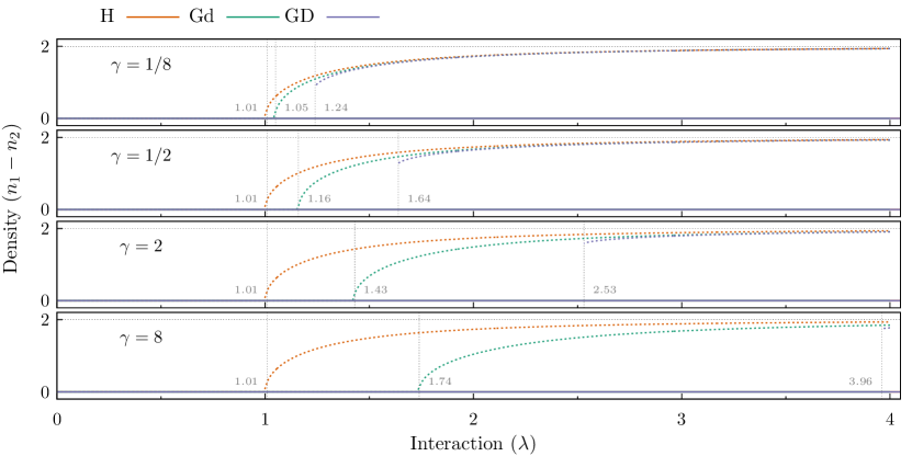
As the first result, we show in Fig. 4 the relative electron density $n_{1}-n_{2}$ as a function of the interaction and adiabatic ratio for the solutions obtained by a symmetric and an asymmetric initial guess, from here on referred to as asymmetric and symmetric solutions. The figure shows that a symmetric guess converges to a solution which has the homogeneous electron density $n_{1}=n_{2}=1$ independent of the approximation and for all parameters considered. An asymmetric guess on the other hand converges for a sufficiently strong interaction to a solution which has an inhomogeneous electron density $n_{1}\neq n_{2}$. Once asymmetric solutions have emerged as a function of the interaction, both types of solutions co-exist for the parameters explored in the present work. The asymmetric solutions have in common that the relative density approaches two as the interaction gets stronger which, similarly to the mean-field case, signals the formation of a localized bipolaron. The manner in which this asymmetric solution appears is however not in common to all approximations. The mean-field approximation, as discussed earlier, breaks the symmetry in the manner of a bifurcation. The same is true for the partially self-consistent approximation, but not for the fully self-consistent approximation in which asymmetric solutions are found to emerge discontinuously from the symmetric solution as a function of the interaction. Additionally, on the contrary to the mean-field case, the value of the interaction at which the asymmetric solution emerges is not independent of the adiabatic ratio, but is pushed to higher interactions $\lambda>1$ in the correlated approximations.

Figure 5: The critical value of interaction $\lambda_{C}$ at which an asymmetric solution emerges as a function of the adiabatic ratio. (color online)

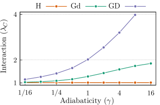
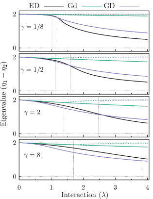
The critical interaction $\lambda_{C}$ below which we do not find an asymmetric solution is shown in Fig. 5 as a function of the adiabatic ratio. This figure shows that the critical point approaches one in the adiabatic limit irrespective of the approximation, while its value depends on the approximation for finite adiabatic ratios and in the anti-adiabatic limit. As the adiabatic ratio is increased, the critical interaction approaches two in the partially self-consistent approximation, which is consistent with the asymptotic limit proposed in Sec. IV.3. In the fully self-consistent approximation, the critical point is shifted to even higher interactions so that for the highest adiabatic ratio $\gamma=16$ we do not find it in the range of interactions $\lambda\in[0,4]$ studied in this work.

The reason why we find a critical interaction below which we can not obtain an asymmetric solution is, in the mean-field case, the fact that we do not allow unphysical complex valued densities. The partially self-consistent approximation has been shown to reduce to the mean-field approximation in the adiabatic and anti-adiabatic limits which suggests that the same reason holds for the partially self-consistent case. On the other hand, we do not know if this is the case for the fully self-consistent approximation. The discussion of the phonon vacuum instability Alexandrov et al. (1994) given in Sec. IV.4 rather supports the view that an asymmetric electron propagator causes a divergence of the phonon propagator, and due to self-consistency we do not find a physical asymmetric solution. However, the symmetric solution does not show any signs of the phonon vacuum instability in the sense that we find a finite solution.

Figure 6: The total energies ($E/T$) for the asymmetric (dashed line) and symmetric (solid line) solutions as a function of the interaction $\lambda$ for different adiabatic ratios $\gamma$. The inset shows the difference $E_{\mathrm{MBPT}}-E_{\mathrm{ED}}$ between approximate (MBPT) and exact (ED) total energies. The dotted vertical lines denote the critical values of interaction $\lambda_{C}$.

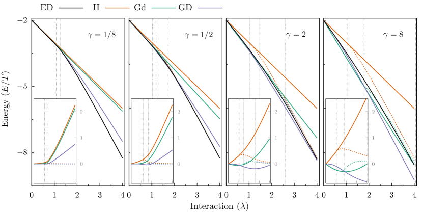
The total energies shown in Fig. 6 in units of the hopping allow us to determine which one of the solutions, symmetric or asymmetric, is the lowest energy solution for a given approximation. These total energies are independent of the adiabatic ratio in the mean-field approximation, and the asymmetric solution is lower than the symmetric solution in the energy. The total energies obtained in either the partially or fully self-consistent approximation are however not independent of the adiabatic ratio. In the adiabatic limit, we find similarly to the mean-field situation that the asymmetric solution is lower in energy once it has emerged. Although this is true for all approximations, adding self-consistency brings the symmetric solution down in energy, especially when the phonon propagator is dressed. As the adiabatic ratio increases, the critical point moves to a higher interaction, and the symmetric solution is lower in energy for a sufficiently high adiabatic ratio. This happens when the total energy becomes lower than the exact total energy. In the anti-adiabatic limit, the symmetric solution is the lowest energy solution in both correlated approximations for the interactions considered in this work.

These results confirm that solutions with inhomogeneous densities exist also in the correlated approximations in which they can be, similarly to the mean-field case, understood to mimic a bipolaron. The critical interaction at which these solutions appear agrees qualitatively in the adiabatic limit with the abrupt formation of a bipolaron in the true ground state, see Sec. IV.1. The approximate solutions however break the symmetry suddenly irrespective of the adiabatic ratio which does not agree with the less abrupt formation of a bipolaronic ground state in the anti-adiabatic limit. The bottom line is that although the asymmetry can be motivated physically, it still does produce inhomogeneity in a homogeneous system. This artefact can be circumvented by constraining ourselves to the homogeneous solution which we find for all parameter values considered here.

IV.6 Comparison With Exact Diagonalization

The many-body approximations used here have been shown to exhibit homogeneous and inhomogeneous densities. The symmetry-broken solution has been attributed to describe a localized bipolaron, while the nature of the symmetric solution has so far remained unclear. In the following, we aim to clarify some physical aspects of both solutions by comparing them energetically with exact diagonalization.

Let us start by taking a closer look at the exact and approximate total energies which are shown in Fig. 6 in units of the hopping. The exact total energies shown in the main panel display roughly linear behavior as a function of the effective interaction for the weak and strong interactions. The slopes of these lines depend on the adiabatic ratio so that for the scaled energy $E/T$, the slope related to the weak interactions is steeper in the anti-adiabatic limit. In the adiabatic limit, these two limiting cases are joined together by an abrupt, smooth change in the slope of the total energy curve while, in the anti-adiabatic limit, this abrupt change is smoothened out and moved to higher values of the interaction. This feature has been shown to correspond to an increase in the binding energy of the bipolaron, see Sec. IV.1, and has been used to signal a crossover to an on-site bipolaron in the more general Hubbard-Holstein model Berciu (2007).

Let us next compare the approximate total energies to the exact total energy starting with the symmetric solutions, and using as help the difference between approximate and exact total energies shown in the inset of Fig. 6. The symmetric mean-field solution does not show any change in the slope of the total energy as a function of the interaction, as seen from Eq. (19). This together with the fact that the total energy is independent of the adiabatic ratio results into a very poor agreement with the exact total energies for all parameters except for the weak interaction adiabatic region. The symmetric partially self-consistent solution shows a change, although almost negligible in comparison to the exact case, in its slope as a function of the interaction. The largest difference to the mean-field case is that the total energy depends on the adiabatic ratio. This qualitative difference leads to a relatively good agreement with the exact results for weak interactions and adiabatic ratios smaller than one, while in the anti-adiabatic cases the total energy is underestimated even for a very weak interaction. The fully self-consistent solution, as opposed to the other symmetric approximate solutions, shows a clear signature of a change in the slope of the total energy, This change appears at the correct values of the interaction, but still underestimates the change of the slope of the exact total energy as a function of $\lambda$. This observation allows us to conclude that out of the symmetric solutions, the fully self-consistent solution is in best agreement with the exact results giving relatively good results for weak- to moderate interactions in the adiabatic limit and weak interactions in the anti-adiabatic limit.

The asymmetric solutions, unlike their symmetric counterparts, show all qualitatively similar behavior as a function of the interaction once they have emerged. The asymmetric solutions appear in the adiabatic regime roughly at the same point in which the slope of the exact total energy changes abruptly. As the critical interaction $\lambda_{C}$ is shifted in the correlated approximations to higher interactions as a function of the adiabatic ratio, it can be said to follow a similar trend as the slope of the exact total energy does, although only the symmetry-breaking can be said to be abrupt in the anti-adiabatic regime. The total energy differences shown in the inset illustrate the fact that all symmetry-broken total energies approach asymptotically to the exact total energy as a function the interaction. This is particularly true in the adiabatic limit in which symmetric total energies are in good agreement at the critical values $\lambda_{C}$, and hence the symmetry-broken total energies are in quantitative agreement with the exact result. The fact that asymmetric total energies are so good in the strong interaction limit is related to the almost degenerate ground and first excited state of the system. A linear combination of these states leads to a symmetry-broken state whose energy however is extremely close to the true total energy Ranninger and Thibblin (1992).

Figure 7: The insets display exact phonon (open circles, $E_{p}/T$), electron (no points, $E_{e}/T$), and electron-phonon interaction (filled circles, $E_{ep}/T$) energies as a function of the interaction $\lambda$ for different adiabatic ratios $\gamma$. The main panels display the differences $E_{\mathrm{MBPT}}-E_{\mathrm{ED}}$ between approximate (MBPT) and exact (ED) energy components for the symmetric (solid line) and asymmetric (dashed line) solutions. The dotted vertical lines denote the critical values of interaction $\lambda_{C}$, and labels next to lines on the left most panel are meant to guide the reader when moving to the panels on the right. (color online)

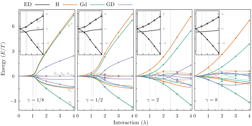
The electron, phonon, and electron-phonon interaction energies are shown for the exact solution in the insets of Fig. 7. The electron energy is $E_{e}/T=\eta_{2}-\eta_{1}$, where $\eta_{1}$ and $\eta_{2}$ are eigenvalues of the spin-summed, one-body reduced density matrix, that is so-called natural occupation numbers Löwdin and Shull (1956). This energy contribution remains almost a constant in the limit of weak interactions, and increases as a function of the interaction roughly as $-2/\lambda$ in the strong interaction case in the adiabatic limit. As the adiabatic ratio is increased, the electron energy changes less abruptly, and shows almost linear increase as a function of the interaction. The exact phonon energy, which is a sum of the classical $E_{pC}/T=\lambda$ and quantum $E_{pQ}\equiv E_{p}-E_{pC}$ contributions, and the electron-phonon interaction energy, which is a sum of the classical $E_{epC}=-2\lambda$ and quantum $E_{pQ}\equiv E_{ep}-E_{epC}$ contributions, show a linear increase and decrease as a function of the interaction in the weak and strong interaction limits, respectively. As for the total energy, the change from the linear behavior for weak interactions to the linear behavior for strong interactions appears abruptly in the adiabatic limit, and as smoothened out and at higher interactions when the adiabatic ratio is increased.

The main panels of Fig. 7 display differences between the approximate and exact energy components as a function of the parameters. Let us first discuss the symmetric solutions which give the classical energy components exactly, as seen from Eq. (3), and therefore the energy differences measure the difference in the quantum contributions. The overall picture here is that these energy components deviate from their exact correspondence more than their sum does, that is the total energy, which implies some kind of error cancellation. The symmetric mean-field and partially self-consistent solutions describe nuclear motion at the mean-field level which means that they fail when the quantum contribution becomes large. Our data shows that the quantum contribution becomes appreciable for all parameters except for the adiabatic weak interaction regime in which these two approximations give a relatively good agreement to the exact phonon energy. In the fully self-consistent case, we however dress the phonon propagator, and therefore gain the ability to capture some of the quantum contribution. This is seen in the figure as an improved agreement with the exact phonon energy for all adiabatic ratios and values of the interactions. The symmetric mean-field solution gives $-2T$ as the electron energy which means that it agrees adequately with exact results only in the adiabatic weak interaction limit in which the exact electron energy remains roughly constant as a function of the interaction. The partially self-consistent approximation incorporates some electron correlation beyond mean-field which is seen as improved agreement with exact results for all adiabatic ratios. The qualitative gain of further introducing self-consistency in the fully self-consistent case is that the electron energy is in a better agreement with the exact result also in the adiabatic limit. The last energy component is the electron-phonon interaction energy which deviates the most from the exact result. As in the case of other energy components, the mean-field solution again fails to give a good agreement with exact results except in the adiabatic weak coupling regime. The partially and especially the fully self-consistent solutions improve on the mean-field picture, so that the latter is again in the best agreement with exact electron-phonon interaction energy for all parameters considered. The error in the interaction energy is of the opposite sign to the error in the phonon energy, mostly also to the electron energy, and therefore leads to the error cancellation observed for the total energy.

Figure 8: The quantum or correlation contributions to the phonon (open circles, $E_{pQ}/T$) and electron-phonon interaction (filled circles, $E_{epQ}/T$) energies for the exact, and asymmetric (dashed line) and symmetric (solid line) solutions as a function of the interaction $\lambda$ for different adiabatic ratios $\gamma$. The dotted vertical lines denote the critical values of interaction $\lambda_{C}$. (color online)

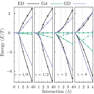
Once the asymmetric solutions appear when the interaction is increased, their energy components behave similarly to one another, as seen for the total energies. Also the trend is the same as for the total energies, that is all energy components approach asymptotically as a function of interaction towards the corresponding exact energy component. There is even a quantitative agreement with the exact energy components for a high enough interaction. Additionally, we find, like in the symmetric case, that there is an error cancellation occurring between the different components. The quantum contributions to the phonon and electron-phonon interaction energies are shown in Fig. 8 for the correlated solutions, and these contributions are by construction identically to zero for the mean-field approximation. This figure shows that an asymmetric solution, irrespective of the approximation, gives quantum energy contributions which tend towards zero as a function of the interaction, and hence the energies consist solely of a classical-like, mean-field contribution.

Figure 9: The difference $\eta_{1}-\eta_{2}$ of the eigenvalues of the spin-summed, electron one-body reduced density matrix for the asymmetric (dashed line) and symmetric (full line) solutions as a function of the interaction ($\lambda$) for different adiabatic ratios ($\gamma$). The dotted vertical lines denote the critical values of interaction $\lambda_{C}$. (color online)

As a last indicator of the physical nature these solutions, we show in Fig. 9 the difference $\eta_{1}-\eta_{2}$ of the eigenvalues of the spin-summed, electron one-body reduced density matrix. This difference is only shown for the exact solution and the correlated approximations since the natural occupation numbers are by construction fixed to $\eta_{1}=2$ and $\eta_{2}=0$ in the mean-field approximation. The figure shows that the difference approaches two as a function of the interaction also for the asymmetric solutions of the correlated approximations. This means that the agreement with the exact electron energy follows through the symmetry-broken eigenvectors of the density matrix. However, this is not the case for the symmetric solutions out of which the fully self-consistent agrees qualitatively with the exact natural occupation numbers. There is also an observation to be made from this figure, namely due to the fact that the particle number is always two, the eigenvalues are between zero and two for all approximate solutions. This shows that the many-body approximation here satisfy an $N$-representability condition Davidson (1976). In the anti-adiabatic limit, the natural occupation numbers can be used to construct the ground-state wave function, and therefore they give invaluable information about the bipolaronic ground state. The first step to make this correspondence is to map the Holstein model to the attractive Hubbard model using the Lang-Firsov transformation Stefanucci and van Leeuwen (2013); Macridin et al. (2004). The Hamiltonian is then given for two electrons by

$$\frac{\hat{H}}{T}= -\lambda+\gamma\sum_{i=1}^{2}\hat{\tilde{a}}_{i}^{\dagger}\hat{\tilde{a}}_{i}-\lambda\sum_{i=1}^{2}\hat{\tilde{n}}_{i\uparrow}\hat{\tilde{n}}_{i\downarrow}$$

$$-\sum_{\sigma}\big{(}\hat{X}_{1}^{\dagger}\hat{X}_{2}\hat{\tilde{c}}_{1\sigma}^{\dagger}\hat{\tilde{c}}_{2\sigma}+\hat{X}_{2}^{\dagger}\hat{X}_{1}\hat{\tilde{c}}_{2\sigma}^{\dagger}\hat{\tilde{c}}_{1\sigma}\big{)}\,,$$

where the transformed operators are

$$\hat{\tilde{a}}_{i} \equiv\hat{a}_{i}+\sqrt{\lambda/2\gamma}\hat{n}_{i}\,,$$

$$\hat{\tilde{c}}_{i} \equiv\hat{X}_{i}\hat{c}_{i}\,,$$

$$\hat{X}_{i} \equiv e^{\sqrt{\lambda/2\gamma}(\hat{a}_{i}^{\dagger}-\hat{a}_{i})}\,,$$

and the density operator $\hat{\tilde{n}}_{i\sigma}\equiv\hat{\tilde{c}}^{\dagger}_{i\sigma}\hat{\tilde{c}}_{i\sigma}$ is defined as usual. If we take the anti-adiabatic limit, or more precisely $\lambda/2\gamma\rightarrow 0$ such that $\lambda$ remains finite Macridin et al. (2004), we arrive at the Hamiltonian

$$\hat{H}_{\mathrm{H}}\equiv -T\lambda+\omega_{0}\sum_{i=1}^{2}\hat{a}_{i}^{\dagger}\hat{a}_{i}-\lambda\sum_{i}\hat{n}_{i\uparrow}\hat{n}_{i\downarrow}$$

$$- T\sum_{\sigma}\big{(}\hat{c}_{2\sigma}^{\dagger}\hat{c}_{1\sigma}+\hat{c}_{1\sigma}^{\dagger}\hat{c}_{2\sigma}\big{)}\,,$$

where the phonon part is just the non-interacting one, and the electronic part is equal to the Hamiltonian operator of the attractive Hubbard model with the interaction $-\lambda$. The ground-state wave function is a product of a zero-phonon state and an electronic wave function which can be written by Löwdin-Shull expansion Löwdin and Shull (1956) as

$$\lvert\Psi_{e}\rangle= \frac{b_{1}+b_{2}}{2}\big{(}\hat{c}^{\dagger}_{1\uparrow}\hat{c}^{\dagger}_{1\downarrow}+\hat{c}^{\dagger}_{2\uparrow}\hat{c}^{\dagger}_{2\downarrow}\big{)}\lvert 0\rangle_{e}$$

$$+\frac{b_{1}-b_{2}}{2}\big{(}\hat{c}^{\dagger}_{1\uparrow}\hat{c}^{\dagger}_{2\downarrow}+\hat{c}^{\dagger}_{2\uparrow}\hat{c}^{\dagger}_{1\downarrow}\big{)}\lvert 0\rangle_{e}\,,$$

where $\lvert 0\rangle_{e}$ is the empty electronic state, and $b_{i}=\sqrt{\eta_{i}/2}$ are called natural amplitudes. In general the coefficients $b_{i}$ are defined up to a sign Giesbertz and van Leeuwen (2013a, b). However, since in this case the ground state can be calculated analytically we can readily determine the signs to be positive in our case. At the limit of strong interactions, the natural occupation numbers approach one which implies that $b_{1}-b_{2}$ approaches zero and therefore the ground-state wave function describes two electrons on the same site, which is the bipolaronic ground state in the anti-adiabatic case. The natural occupation numbers shown for the approximations in the anti-adiabatic case $\gamma=8$ then imply that the fully self-consistent approximation describes a paired two-electron state without symmetry-breaking and localization. The figure also shows that this pairing is overestimated for a wide range of values of the interaction in the intermediate to strong couplings.

The presented results re-enforce the picture that the asymmetric solutions can be seen to describe a classical-like, localized bipolaron. This kind of state is the degenerate ground-state solution in the extreme adiabatic and anti-adiabatic limits obtained by neglecting the nuclear and electron kinetic energies, but not for finite parameters for which degeneracy is broken and the solution is symmetric. On the other hand, we have seen that if we restrict ourselves to a solution which respects this symmetry, only the fully self-consistent approximation shows sufficient indirect evidence that a correlated two-electron state is formed as a function of the interaction. This indirect evidence is further supported by the natural occupation number analysis in the anti-adiabatic limit.

V Conclusion

We have studied the ground-state properties of the homogeneous two-site and two-electron Holstein model. Our study has been conducted using many-body perturbation theory, based on the Hartree, and partially and fully self-consistent Born approximations. We have calculated electron densities, natural occupation numbers, as well as total energies and electron, phonon and electron-phonon interaction energies. We have analyzed the results by analytic and numerical means, and compared them to numerically exact results obtained via exact diagonalization.

The results show that there exists a critical interaction above which the many-body approximations support at least three solutions. One of these solutions is spatially homogeneous while the other two are inhomogeneous in both electron population and nuclear displacement, and therefore break the reflection symmetry of the system. The symmetry-broken electron density approaches two on one of the sites and zero on the other, while the displacement increases and decreases linearly with the electron density, respectively. The energy components and total energies of these solutions have been shown to agree at best quantitatively with exact results, while their quantum contributions approach zero for strong interactions. These observations support the physical picture that the inhomogeneous solutions represent a localized, classical-like bipolaron. The asymmetric solutions are alike irrespective of the approximation, but this is not to the case for the homogeneous solutions. The comparison of the energy components and total energies shows that the homogeneous solutions of the Hartree and partially self-consistent Born approximations do not agree even qualitatively with exact results for intermediate to strong interactions. The fully self-consistent approximation instead does compare well with exact results at least up to intermediate interactions in the adiabatic case, and at least for weak interactions in the anti-adiabatic case. This approximation also shows a significant, although underestimated, change in the slope of the total energy in the adiabatic case $\gamma=1/8$ in a qualitative agreement with the exact solution where we associate this change with a crossover to a bipolaronic state as in Berciu (2007). The homogeneous solution of the fully self-consistent Born approximation is then understood to describe partially a bipolaron crossover in this adiabatic case. A study in an infinite dimensional extended system has shown that this approximation predicts qualitatively a polaronic crossover, but gives only exponentially decaying quasi-particle spectral weight and hence no true bipolaronic metal-insulator transition Capone and Ciuchi (2003). The spin-summed natural occupation numbers obey a trend analogous to the energetics, they approach each other as a function of the interaction in the exact and fully self-consistent Born solutions but do not change as significantly in the less sophisticated approximations. We have shown by mapping the model to the attractive Hubbard model in the anti-adiabatic limit that natural occupation numbers which approach one another indicate the formation of a paired two-electron state. This observation favors a conclusion that the homogeneous solution of the fully self-consistent Born approximation describes a paired two-electron state for the anti-adiabatic case $\gamma=8$ considered here.

The presented results contribute to understanding how these approximations behave in the presence of a strong localizing interaction. In particular, we have shown that the many-body approximations used in this work have multiple physical solutions, and they give rise to spontaneous symmetry-breaking if allowed. These general features appear naturally in the bipolaronic system studied here, and therefore raise a question if these features manifest themselves in dynamical settings, such as in time-dependent quantum transport through molecular junctions, as instable or metastable dynamics. The extension of the present formalism to these cases requires the solution of the two-time Kadanoff-Baym equations for open systems which we have studied extensively in the last few years for the case of purely electronic systems. The next step into this direction is to study how dynamical properties at the level of response functions are described in the many-body approximations discussed here Säkkinen et al. . This knowledge will be of great importance for understanding how the new time-scale related to nuclear motion appears in the transient regime Perfetto and Stefanucci (2013). Lastly, we remark that this may also require further simplifications of the Kadanoff-Baym equations which lead to computationally more favorable single-time equations Pal et al. (2009, 2011); Marini (2013); Balzer et al. (2013); Latini et al. (2014).

Appendix A Energy Functional

The total energies presented in this work are obtained using an energy functional whose derivation will be given below. The underlying idea is that the electron propagator obeys the equation of motion

$$\imath\partial_{z}G_{ij}(z;z^{\prime}) =\delta_{ij}\delta(z,z^{\prime})$$

$$+\sum_{k}h_{ik}G_{kj}(z;z^{\prime})$$

$$-\imath\sum_{kl}M_{ik}^{l}\left\langle\mathcal{T}\left\{\hat{\phi}_{l}(z)\hat{c}_{H;k}(z)\hat{c}^{\dagger}_{H;j}(z^{\prime})\right\}\right\rangle\,,$$

which together with the phonon propagator allow us to write the energy components as

$$E_{p}(z) =\sum_{IJ}\Omega_{IJ}\left\langle\hat{\phi}_{H;I}(z)\hat{\phi}_{H;J}(z)\right\rangle$$

$$=-\frac{1}{\imath}\sum_{IJ}\Omega_{IJ}\big{(}D_{JI}(z,z^{+})-\imath\phi_{I}(z)\phi_{J}(z)\big{)}\,,$$

$$E_{e}(z) =\sum_{ij}h_{ij}\left\langle\hat{c}^{\dagger}_{H;i}(z)\hat{c}_{H;j}(z)\right\rangle$$

$$=\frac{1}{\imath}\sum_{ij}h_{ij}G_{ji}(z,z^{+})\,,$$

$$E_{ep}(z) =\sum_{I}\sum_{jk}M_{jk}^{I}\left\langle\hat{\phi}_{H;I}(z)\hat{c}_{H;j}^{\dagger}(z)\hat{c}_{H;k}(z)\right\rangle$$

$$=\frac{1}{\imath}\sum_{ik}\big{(}\imath\delta_{ik}\partial_{z}-h_{ik}\big{)}G_{ki}(z;z^{\prime})\big{|}_{z^{\prime}=z^{+}}\,,$$

where the subscript $H$ denotes a Heisenberg picture operator. Finally, by combining these results, we find that the total energy can be written as

$$E_{\mathrm{GM}}(z) =\sum_{i}\partial_{z}G_{ii}(z;z^{\prime})\big{|}_{z^{\prime}=z^{+}}$$

$$-\frac{1}{\imath}\sum_{IJ}\Big{(}\Omega_{IJ}\big{(}D_{JI}(z,z^{+})-\imath\phi_{I}(z)\phi_{J}(z)\big{)}\Big{)}\,,$$

and is therefore a functional of the electron and phonon propagators. We call this functional according to its deriving principles Galitski-Migdal functional Galitskii and Migdal (1958); Almbladh et al. (1999); Holm and von Barth (2004).

Appendix B Numerical Details

The numerical method used in the present work to solve the coupled, equilibrium Dyson equations is the widely used method of fixed-point iterations. This method has been previosly described in Stan et al. (2009). Here we extend this approach with some necessary modifications to allow for electron-phonon coupling in the system.

In the present work, the electron and phonon propagators are discretized in the imaginary-time $\tau$ on the geometric grid

$$\tau_{k+1}-\tau_{k}\equiv ab^{k}$$

such that $\tau_{0}=0$ and $\tau_{k}\in[0,\beta/2]$. The grid in the interval $\tau\in[\beta/2,\beta]$ is obtained by mirroring of this grid with respect to $\beta/2$. The grid parameters used here are $a=10^{-3}$ and $b=1.1$, or even smaller. The equations are first rewritten in terms of static electron $g_{\mathrm{s}}^{M}$ and phonon $d_{\mathrm{s}}^{M}$ propagators which satisfy the equations of motion

$$-\big{(}\boldsymbol{\partial}_{\tau}+\boldsymbol{h}-\mu_{\mathrm{s}}\big{)}\boldsymbol{g}_{\mathrm{s}}^{M}(\tau) =\imath\boldsymbol{\delta}(\tau)+\big{[}\boldsymbol{\Sigma}_{\mathrm{s}}^{M}\star\boldsymbol{g}_{\mathrm{s}}^{M}\big{]}(\tau)\,,$$

$$-\big{(}\boldsymbol{\alpha}\partial_{\tau}+\boldsymbol{\omega}\boldsymbol{1}\big{)}\boldsymbol{d}_{\mathrm{s}}^{M}(\tau) =\imath\boldsymbol{\delta}(\tau)+\big{[}\boldsymbol{\Pi}_{\mathrm{s}}^{M}\star\boldsymbol{d}_{\mathrm{s}}^{M}\big{]}(\tau)\,,$$

where $\mu_{\mathrm{s}}$ denotes a static chemical potential, while $\Sigma_{\mathrm{s}}^{M}$ and $\Pi_{\mathrm{s}}^{M}$ denote static self-energies. The word static refers here to the fact that these quantities are independent of the propagators $G^{M}$ and $D^{M}$ which we want to solve. The Dyson equations for these propagators can be then rewritten as

$$\boldsymbol{G}^{M}(\tau) =\boldsymbol{g}_{\mathrm{s}}^{M}(\tau)+\big{[}\boldsymbol{g}_{\mathrm{s}}^{M}\star\boldsymbol{\overline{\Sigma}}^{M}\star\boldsymbol{G}^{M}\big{]}(\tau)\,,$$

$$\boldsymbol{D}^{M}(\tau) =\boldsymbol{d}_{\mathrm{s}}^{M}(\tau)+\big{[}\boldsymbol{d}_{\mathrm{s}}^{M}\star\boldsymbol{\overline{\Pi}}^{M}\star\boldsymbol{D}^{M}\big{]}(\tau)\,,$$

where we defined the effective electron $\boldsymbol{\overline{\Sigma}}_{S}^{M}(\tau)\equiv\boldsymbol{\Sigma}^{M}(\tau)-\boldsymbol{\Sigma}_{\mathrm{s}}^{M}(\tau)+\boldsymbol{\delta}(\tau)\big{(}\mu-\mu_{\mathrm{s}}\big{)}$ and phonon $\boldsymbol{\overline{\Pi}}_{S}^{M}(\tau)\equiv\boldsymbol{\Pi}^{M}(\tau)-\boldsymbol{\Pi}_{\mathrm{s}}^{M}(\tau)$ self-energies.

The method of fixed-point iterations relies on the idea that the solution to the equations is a fixed-point of a mapping which given the propagators as an input gives new propagators as its output. This procedure can be iterated to generate a sequence of propagators which in the ideal case converges to a fixed point of this mapping. This work is based on a scheme in which the propagators of the $k$-th iteration are given as inputs to the mappings

$$\mathcal{F}_{G}:\;\{G,D\} \rightarrow\boldsymbol{g}_{\mathrm{s}}^{M}+\boldsymbol{g}_{\mathrm{s}}^{M}\star\boldsymbol{\overline{\Sigma}}[G,D]\star\boldsymbol{G}\,,$$

$$\mathcal{F}_{D}:\;\{G,D\} \rightarrow\boldsymbol{d}_{\mathrm{s}}^{M}(\tau)+\boldsymbol{d}_{\mathrm{s}}^{M}\star\boldsymbol{\overline{\Pi}}[G]\star\boldsymbol{D}\,,$$

which give a new pair of propagators as its output. This mapping by itself can be unstable, so in order to improve the convergence of this sequence, we have implemented a well-known convergence acceleration method called Direct Inversion of Iterative Subspace (DIIS) Pulay (1980); Thygesen and Rubio (2008). We apply this technique by storing a history of $N$ latest iterates, and constructing new optimized electron and phonon propagators in the $k$-th iteration round according to

$$\boldsymbol{G}_{\mathrm{opt}}^{k}(\tau) =\sum_{\begin{subarray}{c}i=0\\ i\leq k\end{subarray}}^{N}c_{i}\boldsymbol{G}_{k-i}(\tau)\,,$$

$$\boldsymbol{D}_{\mathrm{opt}}^{k}(\tau) =\sum_{\begin{subarray}{c}i=0\\ i\leq k\end{subarray}}^{N}c_{i}\boldsymbol{D}_{k-i}(\tau)\,,$$

where the coefficients $c_{i}$ are fixed by minimizing the residual norm $r_{k}\equiv\left|\left|\boldsymbol{G}_{\mathrm{opt}}^{k}-\mathcal{F}_{G}\big{[}\boldsymbol{G}_{\mathrm{opt}}^{k}\big{]}\right|\right|^{2}+\left|\left|\boldsymbol{D}_{\mathrm{opt}}^{k}-\mathcal{F}_{D}\big{[}\boldsymbol{D}_{\mathrm{opt}}^{k}\big{]}\right|\right|^{2}$ under the constraint that the coefficients $c_{i}$ sum up to unity. The norm is defined in the usual way $\left|\left|\boldsymbol{a}\right|\right|\equiv\sqrt{\langle\boldsymbol{a},\boldsymbol{a}\rangle}$ in terms of the inner product

$$\langle\boldsymbol{a},\boldsymbol{b}\rangle \equiv\int\limits_{0}^{\beta}\!d\tau\;\mathrm{tr}\big{(}\boldsymbol{a}^{\dagger}(\tau)\boldsymbol{b}(\tau)\big{)}$$

where $\boldsymbol{a},\boldsymbol{b}$ are matrix valued Matsubara functions, and $\mathrm{tr}$ denotes the usual matrix trace. To overcome the fact that this optimization problem is inherently non-linear, we make the usual approximation by assuming that the mappings are approximately linear which allows us to write

$$r_{k} \approx\sum_{\begin{subarray}{c}i,j=0\\ i,j\leq k\end{subarray}}^{N}c_{i}^{\dagger}c_{j}r_{k,i}r_{k,j}$$

where we defined the residual norm $r_{k,i}\equiv\left|\left|\boldsymbol{G}_{k-i}-\mathcal{F}_{G}\big{[}\boldsymbol{G}_{k-i}\big{]}\right|\right|^{2}+\left|\left|\boldsymbol{D}_{k-i}-\mathcal{F}_{D}\big{[}\boldsymbol{D}_{k-i}\big{]}\right|\right|^{2}$. This simplified constrained optimization problem leads to the usual set of linear equations

$$\begin{pmatrix}R_{k}^{*}R_{k}^{T}&-1\\ -1&0\end{pmatrix}\begin{pmatrix}C\\ \mu\end{pmatrix}=\begin{pmatrix}\bar{0}\\ -1\end{pmatrix}$$

where $C\equiv(c_{0},\dots,c_{N})^{T}$ and $R_{k}\equiv(r_{k,0},\dots,r_{k,N})^{T}$ are vectors, $T$ denotes the vector transpose, and $\mu$ is a Lagrange multiplier enforcing the equality constraint. Finally, new iterates are given by the linear combinations

$$\boldsymbol{G}_{k+1}^{M} =d\mathcal{F}_{G}[\boldsymbol{G}_{k}^{M}]+(1-d)\boldsymbol{G}_{\mathrm{opt}}^{k}\,,$$

$$\boldsymbol{D}_{k+1}^{M} =d\mathcal{F}_{D}[\boldsymbol{D}_{k}^{M}]+(1-d)\boldsymbol{D}_{\mathrm{opt}}^{k}\,,$$

where $d$ is an empirically chosen damping factor, which is typically fixed to $0.2-1.0$. Although convergence of this iterative sequence is not guaranteed, we have found that it does usually converge to a solution. The convergence criteria used in the present work is that the change of the total energy and the value of the residual norm $r_{k,0}$ are both below the tolerance $10^{-8}$.

References

- Schrieffer (1983) J. R. Schrieffer, Theory of Superconductivity (Perseus Books, 1983).
- Galperin et al. (2007) M. Galperin, M. A. Ratner, and A. Nitzan, J. Phys.: Condens. Matter 19, 103201 (2007).
- Cuevas and Scheer (2010) J. C. Cuevas and E. Scheer, Molecular Electronics: An Introduction to Theory and Experiment (World Scientific, 2010).
- Dash et al. (2010) L. K. Dash, H. Ness, and R. W. Godby, J. Chem. Phys. 132, 104113 (2010).
- Dash et al. (2011) L. K. Dash, H. Ness, and R. W. Godby, Phys. Rev. B 84, 085433 (2011).
- Wilner et al. (2014) E. Y. Wilner, H. Wang, M. Thoss, and E. Rabani, “Nonequilibrium dynamics with electron-phonon interactions: Transient dynamics and approach to steady state,” (2014), arXiv:cond-mat.str-el/1402.6454 .
- Boese and Schoeller (2001) D. Boese and H. Schoeller, Europhys. Lett. 54, 668 (2001).
- Zazunov et al. (2006) A. Zazunov, D. Feinberg, and T. Martin, Phys. Rev. B 73, 115403 (2006).
- Alexandrov and Bratkovsky (2003) A. S. Alexandrov and A. M. Bratkovsky, Phys. Rev. B 67, 235312 (2003).
- Myöhänen et al. (2012) P. Myöhänen, R. Tuovinen, T. Korhonen, G. Stefanucci, and R. van Leeuwen, Phys. Rev. B 85, 075105 (2012).
- Jin and Thygesen (2014) C. Jin and K. S. Thygesen, Phys. Rev. B 89, 041102 (2014).
- Perfetto and Stefanucci (2013) E. Perfetto and G. Stefanucci, Phys. Rev. B 88, 245437 (2013).
- Kartsev et al. (2014) A. Kartsev, C. Verdozzi, and G. Stefanucci, Eur. Phys. J. B 87, 1 (2014).
- Alexandrov et al. (2003) A. S. Alexandrov, A. M. Bratkovsky, and R. S. Williams, Phys. Rev. B 67, 075301 (2003).
- Galperin et al. (2008) M. Galperin, A. Nizzan, and M. A. Ratner, J. Phys.: Condens. Matter 20, 374107 (2008).
- Albrecht et al. (2012) K. F. Albrecht, H. Wang, L. M. Uhlbacher, M. Thoss, and A. Komnik, Phys. Rev. B 86, 081412 (2012).
- Wilner et al. (2013) E. Y. Wilner, H. Wang, G. Cohen, M. Thoss, and E. Rabani, Phys. Rev. B 88, 045137 (2013).
- Khosravi et al. (2012) E. Khosravi, A.-M. Uimonen, A. Stan, G. Stefanucci, S. Kurth, R. van Leeuwen, and E. K. U. Gross, Phys. Rev. B 85, 075103 (2012).
- Myöhänen et al. (2008) P. Myöhänen, A. Stan, G. Stefanucci, and R. van Leeuwen, Europhys. Lett. 84, 67001 (2008).
- Myöhänen et al. (2009) P. Myöhänen, A. Stan, G. Stefanucci, and R. van Leeuwen, Phys. Rev. B 80, 115107 (2009).
- Stefanucci and van Leeuwen (2013) G. Stefanucci and R. van Leeuwen, Nonequilibrium Many-Body Theory of Quantum Systems: A Modern Introduction (Cambridge, 2013).
- Dahlen and van Leeuwen (2007) N. E. Dahlen and R. van Leeuwen, Phys. Rev. Lett. 98, 153004 (2007).
- (23) N. Säkkinen, Y. Peng, H. Appel, and R. van Leeuwen, In preparation .
- Fehske and Trugman (2007) H. Fehske and S. Trugman, in Polarons in Advanced Materials, Springer Series in Materials Science, Vol. 103, edited by A. Alexandrov (Springer Netherlands, 2007) pp. 393–461.
- Holstein (2000) T. Holstein, Ann. Phys. 281, 706–724 (2000).
- Devreese and Alexandrov (2009) J. T. Devreese and A. S. Alexandrov, Rep. Prog. Phys. 72, 066501 (2009).
- Hannewald et al. (2004) K. Hannewald, V. M. Stojanović, J. M. T. Schellekens, P. A. Bobbert, G. Kresse, and J. Hafner, Phys. Rev. B 69, 075211 (2004).
- Hannewald and Bobbert (2004) K. Hannewald and P. A. Bobbert, Phys. Rev. B 69, 075212 (2004).
- Schmidt and Schreiber (1987) W. Schmidt and M. Schreiber, J. Chem. Phys. 86, 953 (1987).
- Feinberg et al. (1990) D. Feinberg, S. Ciuchi, and F. de Pasquale, Int. J. Mod. Phys. B 04, 1317 (1990).
- Ranninger and Thibblin (1992) J. Ranninger and U. Thibblin, Phys. Rev. B 45, 1991 (1992).
- Alexandrov et al. (1994) A. S. Alexandrov, V. V. Kabanov, and D. K. Ray, Phys. Rev. B 49, 9915 (1994).
- Marsiglio (1995) F. Marsiglio, Physica C 244, 21 (1995).
- de Mello and Ranninger (1997) E. V. L. de Mello and J. Ranninger, Phys. Rev. B 55, 14872 (1997).
- Crljen (1998) Ž. Crljen, Fizika A 7, 75 (1998).
- Rongsheng et al. (2002) H. Rongsheng, L. Zijing, and W. Kelin, Phys. Rev. B 65, 174303 (2002).
- Qing-Bao and Qing-Hu (2005) R. Qing-Bao and C. Qing-Hu, Comm. Theor. Phys. 43, 357 (2005).
- Paganelli and Ciuchi (2008) S. Paganelli and S. Ciuchi, Eur. Phys. J. Special Topics 160, 343 (2008).
- Paganelli and Cuichi (2008) S. Paganelli and S. Cuichi, J. Phys. Condensed Matter 20, 235203 (2008).
- Firsov and Kudinov (1997) Y. A. Firsov and E. K. Kudinov, Phys. Solid State 39, 1930 (1997).
- Chatterjee and Das (2000) J. Chatterjee and A. N. Das, Phys. Rev. B 61, 4592 (2000).
- Gunnarsson et al. (1994) O. Gunnarsson, V. Meden, and K. Schonhammer, Phys. Rev. B 50, 10462 (1994).
- Dahlen and van Leeuwen (2005) N. E. Dahlen and R. van Leeuwen, J. Chem. Phys. 122, 164102 (2005).
- Säkkinen et al. (2012) N. Säkkinen, M. Manninen, and R. van Leeuwen, New. J. Phys. 14, 0132032 (2012).
- Marsiglio (1990) F. Marsiglio, Phys. Rev. B 42, 2416 (1990).
- Freericks (1994) J. K. Freericks, Phys. Rev. B 50, 403 (1994).
- Capone and Ciuchi (2003) M. Capone and S. Ciuchi, Phys. Rev. Lett. 91, 186405 (2003).
- Goodvin et al. (2006) G. L. Goodvin, M. Berciu, and G. A. Sawatzky, Phys. Rev. B 74, 245104 (2006).
- Bauer et al. (2011) J. Bauer, J. E. Han, and O. Gunnarsson, Phys. Rev. B 84, 184531 (2011).
- Holm and von Barth (1998) B. Holm and U. von Barth, Phys. Rev. B 57, 2108 (1998).
- Stan et al. (2006) A. Stan, N. E. Dahlen, and R. van Leeuwen, EPL (Europhysics Letters) 76, 298 (2006).
- Caruso et al. (2013) F. Caruso, P. Rinke, X. Ren, A. Rubio, and M. Scheffler, Phys. Rev. B 88, 075105 (2013).
- Baym and Kadanoff (1961) G. Baym and L. P. Kadanoff, Phys. Rev. 124, 287 (1961).
- Baym (1962) G. Baym, Phys. Rev. 127, 1391 (1962).
- Alexandrov (2001) A. S. Alexandrov, EPL (Europhysics Letters) 56, 92 (2001).
- Tandetzky et al. (2012) F. Tandetzky, J. K. Dewhurst, S. Sharma, and E. K. U. Gross, “Multiplicity of solutions to gw-type approximations,” (2012), arXiv:cond-mat.str-el/1205.4274 .
- Mahan (2000) G. Mahan, Many-Particle Physics, 3rd edition (Springer, 2000).
- Bruus and Flensberg (2004) H. Bruus and K. Flensberg, Many-Body Quantum Theory in Condensed Matter Physics: An Introduction (Oxford Press, 2004).
- Migdal (1958) A. B. Migdal, Zh. Eksp. Teor. Fiz. 34, 1438 (1958), [Sov. Phys. JETP, 7, 996 (1958)].
- Eliashberg (1960a) G. M. Eliashberg, M., Zh. Eksp. Teor. Fiz. 38, 966 (1960a), [Sov. Phys. JETP, 11, 696 (1960)].
- Eliashberg (1960b) G. M. Eliashberg, M., Zh. Eksp. Teor. Fiz. 39, 1437 (1960b), [Sov. Phys. JETP, 12, 1000 (1960)].
- Lang and Firsov (1962) I. G. Lang and Y. A. Firsov, Zh. Eksp. Teor. Fiz. 43, 1843 (1962), [Sov. Phys. JETP 16, 1301 (1962)].
- Helgaker et al. (2000) T. Helgaker, P. Jørgensen, and J. Olsen, Molecular electronic structure theory (Wiley, Chichester, 2000).
- Reimann and Manninen (2002) S. M. Reimann and M. Manninen, Rev. Mod. Phys. 74, 1283 (2002).
- Ivanov (2002) M. Ivanov, “Quantum phase transition in the Hartree-Fock wave function of the hydrogen molecule,” (2002), arXiv:physics/0206036 .
- Alexandrov and Mott (1994) A. S. Alexandrov and N. F. Mott, High Temperature Superconductors and Other Superfluids (Taylor & Francis, 1994).
- Berciu (2007) M. Berciu, Phys. Rev. B 75, 081101 (2007).
- Löwdin and Shull (1956) P.-O. Löwdin and H. Shull, Phys. Rev. 101, 1730 (1956).
- Davidson (1976) E. R. Davidson, Reduced Density Matrices in Quantum Chemistry (Academic Press, New York, 1976).
- Macridin et al. (2004) A. Macridin, G. A. Sawatzky, and M. Jarrell, Phys. Rev. B 69, 245111 (2004).
- Giesbertz and van Leeuwen (2013a) K. J. H. Giesbertz and R. van Leeuwen, J. Chem- Phys- 139, 104109 (2013a).
- Giesbertz and van Leeuwen (2013b) K. J. H. Giesbertz and R. van Leeuwen, J. Chem. Phys. 139, 104110 (2013b).
- Pal et al. (2009) G. Pal, Y. Pavlyukh, H. C. Schneider, and W. Hübner, Eur. Phys. J. B 70, 483 (2009).
- Pal et al. (2011) G. Pal, Y. Pavlyukh, W. Hübner, and H. C. Schneider, Eur. Phys. J. B 79, 327 (2011).
- Marini (2013) A. Marini, J. Phys: Conf. Proc. 427, 012003 (2013).
- Balzer et al. (2013) K. Balzer, S. Hermanns, and M. Bonitz, J. Phys: Conf. Proc. 427, 012006 (2013).
- Latini et al. (2014) S. Latini, E. Perfetto, A.-M. Uimonen, R. van Leeuwen, and G. Stefanucci, Phys. Rev. B 89, 075306 (2014).
- Galitskii and Migdal (1958) V. Galitskii and A. Migdal, Sov. Phys. JETP 7, 96 (1958).
- Almbladh et al. (1999) C.-O. Almbladh, U. von Barth, and R. van Leeuwen, Int. J. Mod. Phys. B 13, 535 (1999).
- Holm and von Barth (2004) B. Holm and U. von Barth, Phys. Scripta T109, 135 (2004).
- Stan et al. (2009) A. Stan, N. E. Dahlen, and R. van Leeuwen, J. Chem. Phys. 130, 114105 (2009).
- Pulay (1980) P. Pulay, J. Chem. Phys. Lett. 73, 393 (1980).
- Thygesen and Rubio (2008) K. S. Thygesen and A. Rubio, Phys. Rev. B 77, 115333 (2008).