Efficient maximum likelihood estimation for Lévy-driven Ornstein–Uhlenbeck processes

Abstract

We consider the problem of efficient estimation of the drift parameter of an Ornstein–Uhlenbeck type process driven by a Lévy process when high-frequency observations are given. The estimator is constructed from the time-continuous likelihood function that leads to an explicit maximum likelihood estimator and requires knowledge of the continuous martingale part. We use a thresholding technique to approximate the continuous part of the process. Under suitable conditions, we prove asymptotic normality and efficiency in the Hájek–Le Cam sense for the resulting drift estimator. Finally, we investigate the finite sample behavior of the method and compare our approach to least squares estimation.

1 Introduction

Let $(L_{t},t\geq 0)$ be a Lévy process on a filtered probability space $(\Omega,\mathcal{F},(\mathcal{F}_{t}),P)$ adapted to the filtration $(\mathcal{F}_{t})_{t\geq 0}$. Denote by $(b,\sigma^{2},\mu)$ the Lévy–Khintchine triplet of $L$. We call for every $a\in\mathbb{R}$ a strong solution $X$ to the stochastic differential equation

$$\mathrm{d}X_{t}=-aX_{t}\,\mathrm{d}t+\mathrm{d}L_{t},\qquad t\in\mathbb{R}_{+},\qquad X_{0}=\tilde{X},$$ (1)

a Lévy-driven Ornstein–Uhlenbeck (OU) process or Ornstein–Uhlenbeck type process. The initial condition $\tilde{X}$ is assumed to be independent of $L$. We consider the problem of estimating the mean reversion parameter $a$ when observations $X_{t_{1}},\ldots,X_{t_{n}}$ on an interval $[0,T_{n}]$ are given. It is well known that the drift of $X$ is identifiable only in the limit $T_{n}\to\infty$, even when time-continuous observations are given. Therefore, we work under the asymptotic scheme $T_{n}\to\infty$ and $\Delta_{n}=\max_{1\leq i\leq n-1}\{|t_{i+1}-t_{i}|\}\downarrow 0$ as $n\to\infty$.

The OU process serves us here as a toy model to understand the interplay of jumps and continuous component of $X$ in this estimation problem. This interplay is fundamental also for drift estimation in more general models (cf. [18]).

Ornstein–Uhlenbeck type processes have important applications in various fields. In mathematical finance they are well know as a main building block of the Barndorff–Nielsen–Shephard stochastic volatility model (cf. [3]). But also in neuroscience they are popular for the description of the membrane potential of a neuron (cf. [11] and [17]).

Estimation of Lévy-driven Ornstein–Uhlenbeck processes has been considered by several authors (see [22] and the references therein) mostly when the driving Lévy process is a subordinator. Some examples are [13] on nonparametric estimation of the Lévy density of $L$, in [4] the Davis–McCormick estimator was applied in the OU context and parametric estimation based on a cumulant $M$-estimator was studied in [12]. In [8], least squares estimation of the drift parameter for an $\alpha$-stable driver is discussed, when no Gaussian component is present. Reference [22] found that the rate of convergence of the least absolute deviation estimator is either the standard parametric rate, when $L$ has a Gaussian component, or is faster than the standard rate, when $L$ is a pure jump process and depends on the activity of the jumps. In [25], joint parametric estimation of the drift and the Lévy measure was treated via estimating functions. Unfortunately, none of these methods lead to an efficient estimator of the drift when $L$ is a general Lévy process.

To construct an efficient estimator, our starting point will be the continuous time likelihood function. From this likelihood function, an explicit maximum likelihood estimator can be derived, which is efficient in the sense of the Hájek–Le Cam convolution theorem. In the likelihood function the continuous martingale part of $X$ under the dominating measure appears, which is not directly observed in our setting. For discrete observations, we approximate the continuous part of $X$ by neglecting increments that are larger than a certain threshold that has to be chosen appropriately. We will call this thresholding technique a jump filter. For this discretized likelihood estimator with jump filtering, we prove asymptotic normality and efficiency by showing that it attains the same asymptotic distribution as the benchmark estimator based on time-continuous observations.

This leads to the main mathematical question underlying this estimation problem. Can we recover the continuous part of $X$ in the high-frequency limit via jump filtering? If $L$ has only compound Poisson jumps it is intuitively clear that the answer is yes. But when $L$ has infinitely many small jumps in every finite interval this is a much more challenging question. It turns out that even in this situation jump filtering works under mild assumptions on the behavior of the Lévy measure around zero. The main condition here is that the Blumenthal–Getoor index of the jump part is strictly less than two, which is apparently a necessary condition in this context. In this setting, jump filtering becomes possible since on a small time scale increments of the continuous part and of the jump part exhibit a different order of magnitude such that they can be distinguished via thresholding. To control the small jumps of $L$ under thresholding, we derive an estimate for the Markov generator of a thresholded pure jump Lévy process. Estimates of this type without thresholding were given, among others, in [7] and [10].

The problem of separation between continuous and jump part of a process appears naturally in many situations. For example, in estimation of the integrated volatility of a jump diffusion process via realized volatility the quadratic variation of the jump component has to be removed. This problem has been solved by thresholding in [19] for Poisson jumps and in [20] for more general jump behavior. Efficiency questions in this context in a simple parametric model have been addressed in [1]. When properties of the jump component are of interest thresholding techniques are equally useful as demonstrated, among others, in [2]. In contrast to our discussion all these references consider the separation problem for a finite and fixed observation horizon $T_{n}=T<\infty$.

We also demonstrate in a simulation example that jump filtering leads to a major improvement of the drift estimate for finite sample size. Let us also mention that implementation of the drift estimator is straightforward and computation time is not an issue even for large data sets.

The paper is organized as follows: in Section 2 we derive the maximum likelihood estimator based on time-continuous observations, give its asymptotic properties and obtain the efficient limiting distribution for this estimation problem. Section 3 deals with estimating the drift parameter from discrete observations when $L$ has finite jump activity. In Section 4 we build on the results from Sections 2 and 3 to prove efficiency also for possibly infinite jump activity. The finite sample behavior of the estimator is investigated in Section 5 based on simulated data together with an analysis of the impact of the jump filter on the performance of the estimator.

2 Maximum likelihood estimation

Let us summarize some important facts on Ornstein–Uhlenbeck type processes. It follows from Itô’s formula that an explicit solution of (1) is given by

$$X_{t}=\mathrm{e}^{-at}X_{0}+\int_{0}^{t}\mathrm{e}^{-a(t-s)}\,\mathrm{d}L_{s},\qquad t\in\mathbb{R}_{+}.$$ (2)

The integral in (2) can by partial integration be defined path-wise as a Riemann–Stieltjes integral, since the integrand is of finite variation (see [6], e.g.). This solution to equation (1) is unique up to indistinguishability.

When $L$ is non-deterministic it was shown in [9] that equation (1) admits a causal stationary solution (cf. also [21] and [24]) if and only if

$$\int_{|x|>1}{\log}|x|\mu(\mathrm{d}x)<\infty\quad\mbox{and}\quad a>0.$$ (3)

Under these conditions $X$ has a unique invariant distribution $G$ and $X_{t}\stackrel{{\scriptstyle\mathcal{D}}}{{\longrightarrow}}X_{\infty}\sim G$ as $t\to\infty$.

The Ornstein–Uhlenbeck process $X$ exhibits a modification with càdlàg paths and hence it induces a measure $P^{a}$ on the space $D[0,\infty)$ of càdlàg functions on the interval $[0,\infty)$. Denote by $P_{t}^{a}$ the restriction of $P^{a}$ to the $\sigma$-field $\mathcal{F}_{t}$. If $\sigma^{2}>0$ then these induced measure are locally equivalent (cf. [26]) and the corresponding Radon–Nikodym derivative or likelihood function is given by

$$\frac{\mathrm{d}P_{t}^{a}}{\mathrm{d}P_{t}^{0}}=\exp\biggl{(}-\frac{a}{\sigma^{2}}\int_{0}^{T}X_{s}\,\mathrm{d}X_{s}^{c}-\frac{a^{2}}{2\sigma^{2}}\int_{0}^{T}X_{s}^{2}\,\mathrm{d}s\biggr{)},$$

where $X^{c}$ denotes the continuous $P^{0}$-martingale part of $X$. This leads to the explicit maximum likelihood estimator

$$\hat{a}_{T}=-\frac{\int_{0}^{T}X_{s}\,\mathrm{d}X_{s}^{c}}{\int_{0}^{T}X_{s}^{2}\,\mathrm{d}s}$$ (4)

for $a$ when the process is fully observed on $[0,T]$. The estimator $\hat{a}_{T}$ cannot be applied in this form, since time-continuous observations are usually not available in most applications. Therefore, we will develop in the next section a discrete version of $\hat{a}_{T}$ and prove its efficiency. The main challenge there will be that the continuous part $X^{c}$ is not directly observed and hence has to be approximated from discrete observations of $X$ via jump filtering.

However, for us $\hat{a}_{T}$ will serve as a benchmark for the estimation problem with discrete observations. Asymptotic normality and efficiency in the Hájek–Le Cam sense of $\hat{a}_{T}$ follow easily from general results for exponential families of stochastic processes (cf. [16] and [18]). These results provide an efficiency bound for the case of discrete observations in the next section. Let us summarize them in the following theorem.

Theorem 2.1

(i) Under the condition $\sigma^{2}>0$ the estimator $\hat{a}_{T}$ exists uniquely and is strongly consistent under $P^{a}$, that is,

$$\hat{a}_{T}\stackrel{{\scriptstyle a.s.}}{{\longrightarrow}}a$$

under $P^{a}$ as $T\to\infty$.

i(ii) Suppose that additionally (3) holds and that $X$ has bounded second moments such that the invariant distribution satisfies $E_{a}[X_{\infty}^{2}]<\infty$. Then under $P^{a}$

$$\sqrt{T}(\hat{a}_{T}-a)\stackrel{{\scriptstyle\mathcal{D}}}{{\longrightarrow}}N\biggl{(}0,\frac{\sigma^{2}}{E_{a}[X_{\infty}^{2}]}\biggr{)}$$

and

$$\sigma^{-1}S_{T}^{1/2}(\hat{a}_{T}-a)\stackrel{{\scriptstyle\mathcal{D}}}{{\longrightarrow}}N(0,1)$$ (5)

as $T\to\infty$, where $S_{T}=\int_{0}^{T}X_{s}^{2}\,\mathrm{d}s$.

(iii) The statistical experiment $\{P^{a},a\in\mathbb{R}_{+}\}$ is locally asymptotically normal.

 (iv) The estimator $\hat{a}_{T}$ is asymptotically efficient in the sense of Hájek–Le Cam.

For a proof we refer to [18], Section 4.2.

Remark 2.2.

When $\sigma^{2}$ is known or a consistent estimator is at hand, we can use (5) to construct confidence intervals for $a$.

3 Discrete observations: Finite activity

In this section, we consider the estimation of $a$ for discrete observations. The maximum likelihood estimator for the drift given in (4) involves the continuous martingale part that is unknown when only discrete observations are given. Hence, we will approximate the continuous part of the process by removing observations that most likely contain jumps. We restrict our attention in this section to the case that the driving Lévy process has jumps of finite activity. The jump filtering technique provides us in the high-frequency limit an asymptotically normal and efficient estimator. Based on these results, we will treat the general case of an infinitely active jump component in Section 4.

3.1 Estimator and observation scheme

Let $X$ be an Ornstein–Uhlenbeck process defined by (1) and suppose we observe $X$ at discrete time points $0=t_{1}<t_{2}<\cdots<t_{n}=T_{n}$ such that $T_{n}\to\infty$ as well as $\Delta_{n}=\max_{1\leq i\leq n-1}\{|t_{i+1}-t_{i}|\}\downarrow 0$ and $n\Delta_{n}T_{n}^{-1}=\mathrm{O}(1)$ as $n\to\infty$. The last condition assures that the number of observations $n$ does not grow faster than $T_{n}\Delta_{n}^{-1}$. It can always be fulfilled by neglecting observations and will simplify the formulation of the proof considerably. Denote by $(b,\sigma^{2},\mu)$ the Lévy–Khintchine triplet of $L$. Assume throughout this section that $\lambda=\mu(\mathbb{R})<\infty$ for the Lévy measure $\mu$.

By deleting increments that are larger than a threshold $v_{n}>0$ we filter increments that most likely contain jumps and thus approximate the continuous part with the remaining increments. Applied to the time-continuous likelihood estimator (4) this method leads to the following estimator:

$$\bar{a}_{n}:=-\frac{\sum_{i=0}^{n-1}X_{t_{i}}\Delta_{i}X\mathbf{1}_{\{|\Delta_{i}X|\leq v_{n}\}}}{\sum_{i=0}^{n-1}X_{t_{i}}^{2}(t_{i+1}-t_{i})}.$$ (6)

Here $v_{n}>0,n\in\mathbb{N}$, is a cut-off sequence that will be chosen as a function of the maximal distance between observations $\Delta_{n}$ and $\Delta_{i}X=X_{t_{i+1}}-X_{t_{i}}$.

In the finite activity case, the jump part $J$ of $L$ can be written as a compound Poisson process

$$J_{t}=\sum_{i=1}^{N_{t}}Z_{i},$$

where $N$ is a Poisson process with intensity $\lambda$ and the jump heights $Z_{1},Z_{2},\ldots$ are i.i.d. with distribution $F$.

3.2 Asymptotic normality and efficiency

The indicator function that appears in $\bar{a}_{n}$ deletes increments that are larger than $v_{n}$. In [19], it was shown that increments of the continuous part of $X$ over an interval of length $\Delta_{n}$ are with high probability smaller than $\Delta_{n}^{1/2}$. Hence, we set $v_{n}=\Delta_{n}^{\beta}$ for $\beta\in(0,1/2)$ to keep the continuous part in the limit unaffected by the threshold. In order to be able to choose $v_{n}$ such that $X^{c}_{n}=\sum_{i=0}^{n-1}\Delta_{i}X\mathbf{1}_{\{|\Delta_{i}X|\leq v_{n}\}}$ approximates the continuous martingale part in the limit, we make the following assumptions on the jumps of $L$ and the observation scheme.

Assumption 3.1.

(i) Suppose that $\mu$ and $a$ satisfy (3), the drift $b=0$, the process $X$ has bounded second moments,

i(ii) the distribution $F$ of the jump heights is such that

$$F\bigl{(}\bigl{(}-2\Delta_{n}^{\beta},2\Delta_{n}^{\beta}\bigr{)}\bigr{)}=\mathrm{o}\bigl{(}T_{n}^{-1}\bigr{)},$$

(iii) and there exists $\beta\in(0,1/2)$ such that the maximal distance between observations satisfies $T_{n}\Delta_{n}^{(1-2\beta)\wedge({1/2})}=\mathrm{o}(1)$.

Remark 3.2.

Suppose that $F$ has a bounded Lebesgue density $f$. Then

$$F\bigl{(}\bigl{(}-\Delta_{n}^{\beta},\Delta_{n}^{\beta}\bigr{)}\bigr{)}=\mathrm{O}\bigl{(}\Delta_{n}^{\beta}\bigr{)}$$

and Assumption 3.1(ii) becomes $\Delta_{n}^{\beta}T_{n}=\mathrm{o}(1)$. Together with Assumption 3.1(i), we obtain that $\beta=1/3$ leads to an optimal compromise between Assumption 3.1(i) and (ii).

Remark 3.3.

Assumption 3.1(iii) means here that for given $T_{n}\to\infty$ we require $\Delta_{n}\downarrow 0$ fast enough such that there exists $\beta\in(0,1/2)$:

$$T_{n}\Delta_{n}^{1-2\beta}=\mathrm{o}(1)\quad\mbox{and}\quad T_{n}\Delta_{n}^{1/2}=\mathrm{o}(1).$$

Of course one of these two conditions will be dominating and determine the order of $\Delta_{n}$.

Remark 3.4.

Assumption 3.1(ii) gives a lower bound for the choice of the threshold $\beta$. At the same time Assumption 3.1(iii) limits the range of possible $\beta$’s from above, since the available frequency of observations, that is, the order of $\Delta_{n}$, may be limited in specific applications. Hence, the distribution $F$, the observation length $T_{n}$ and frequency $\Delta_{n}$ fix a range for the choice of $\beta$. At this point the question of a data driven method to choose $\beta$ arises, but this will not be considered in this work. The condition $b=0$ is necessary in this context, since otherwise there is no hope to recover the continuous martingale part via jump filtering.

The following theorem gives as the main result of this section a central limit theorem for the discretized MLE with jump filter.

Theorem 3.5

Suppose that Assumption 3.1 holds and $\sigma^{2}>0$. Set $v_{n}=\Delta_{n}^{\beta}$ for $\beta\in(0,1/2)$, then

$$T_{n}^{1/2}(\bar{a}_{n}-a)\stackrel{{\scriptstyle\mathcal{D}}}{{\longrightarrow}}N\biggl{(}0,\frac{\sigma^{2}}{E_{a}[X_{\infty}^{2}]}\biggr{)}\qquad\mbox{as $n\to\infty$}.$$

The estimator $\bar{a}_{n}$ is asymptotically efficient.

Remark 3.6.

Asymptotic efficiency follows immediately from Theorem 2.1 and the first statement of Theorem 3.5.

3.3 Proofs

We divide the proof of the theorem into several lemmas. First of all, we need a probability bound for the event that the continuous component of $X$ exceeds a certain threshold.

By the Lévy–Itô decomposition (cf. [23]) and since $b=0$ in our setting the driving Lévy process can be decomposed as $L=W+J$, where $W$ is a standard Wiener process and $J$ is a pure jump Lévy process independent of $W$. Denote by $D$ the drift component of $X$, that is,

$$D_{t}=-a\int_{0}^{t}X_{s}\,\mathrm{d}s.$$

Lemma 3.7

Let $\sup_{s\geq 0}\{E[|X_{s}|^{l}]\}<\infty$ for some $l\geq 1$. For any $\delta\in(0,1/2)$ and $i\in\{1,\ldots,n-1\}$, we have

$$P\bigl{(}|\Delta_{i}W+\Delta_{i}D|>\Delta_{n}^{1/2-\delta}\bigr{)}=\mathrm{O}\bigl{(}\Delta_{n}^{l(1/2+\delta)}\bigr{)}\qquad\mbox{as $n\to\infty$}.$$

Proof.

In the first step, we separate $\Delta_{i}W$ and $\Delta_{i}D$:

$$P\bigl{(}|\Delta_{i}W+\Delta_{i}D|>\Delta_{n}^{1/2-\delta}\bigr{)}\leq P\biggl{(}|\Delta_{i}W|>\frac{\Delta_{n}^{1/2-\delta}}{2}\biggr{)}+P\biggl{(}|\Delta_{i}D|>\frac{k\Delta_{n}^{1/2}}{2}\biggr{)}.$$

By Lemma 22.2 in [15],

$$P\biggl{(}|\Delta_{i}W|>\frac{\Delta_{n}^{1/2-\delta}}{2}\biggr{)}\leq 2\Delta_{n}^{\delta}\mathrm{e}^{-{1}/({8\Delta_{n}^{\delta}})}.$$

It follows from Jensen’s inequality that

$$\biggl{|}\int_{t_{i}}^{t_{i+1}}X_{s}\,\mathrm{d}s\biggr{|}^{l}\leq\Delta_{n}^{l-1}\int_{t_{i}}^{t_{i+1}}|X_{s}|^{l}\,\mathrm{d}s.$$

This leads to

$$E\bigl{[}|\Delta_{i}D|^{l}\bigr{]}\leq\Delta_{n}^{l-1}a^{l}\int_{t_{i}}^{t_{i+1}}E\bigl{[}|X_{s}|^{l}\bigr{]}\,\mathrm{d}s\leq\Delta_{n}^{l}a^{l}\sup_{s\in[t_{i},t_{i+1}]}\bigl{\{}E\bigl{[}|X_{s}|^{l}\bigr{]}\bigr{\}}.$$

Finally, Markov’s inequality yields

$$P\biggl{(}|\Delta_{i}D|>\frac{\Delta_{n}^{1/2-\delta}}{2}\biggr{)}\leq a^{l}\sup_{s\in[t_{i},t_{i+1}]}\bigl{\{}E\bigl{[}|X_{s}|^{l}\bigr{]}\bigr{\}}\frac{2^{l}\Delta_{n}^{l}}{\Delta_{n}^{l(1/2-\delta)}}=\mathrm{O}\bigl{(}\Delta_{n}^{l(1/2+\delta)}\bigr{)}.$$

∎

3.3.1 Jump filtering

First, we will investigate how to choose the cut-off sequence $v_{n}$ in order to filter the jumps. Define for $n\in\mathbb{N}$ and $i\in\{1,\ldots,n\}$ the following sequence of events

$$A_{n}^{i}=\bigl{\{}\omega\in\Omega\colon\ \mathbf{1}_{\{|\Delta_{i}X|\leq v_{n}\}}(\omega)=\mathbf{1}_{\{\Delta_{i}N=0\}}(\omega)\bigr{\}}.$$

Here $N$ denotes the counting measure that counts the jumps of $L$.

Lemma 3.8

Suppose that Assumption 3.1 holds and set $v_{n}=\Delta_{n}^{\beta},\beta\in(0,1/2)$, then it follows that for $A_{n}=\bigcap_{i=1}^{n}A_{n}^{i}$ we have

$$P(A_{n})\to 1\qquad\mbox{as $n\to\infty$.}$$

Proof.

Observe that

$$P\bigl{(}A_{n}^{c}\bigr{)}=P\Biggl{(}\bigcup_{i=1}^{n}\bigl{(}A_{n}^{i}\bigr{)}^{c}\Biggr{)}\leq\sum_{i=1}^{n}P\bigl{(}\bigl{(}A_{n}^{i}\bigr{)}^{c}\bigr{)}.$$

By setting

$$K_{n}^{i} = {\bigl{\{}|\Delta_{i}X|\leq v_{n}\bigr{\}}},$$

$$M_{n}^{i} = {\{\Delta_{i}N=0\}},$$

we can rewrite $(A_{n}^{i})^{c}$ as

$$\bigl{(}A_{n}^{i}\bigr{)}^{c}=\{\mathbf{1}_{K_{n}^{i}}\neq\mathbf{1}_{M_{n}^{i}}\}=\bigl{(}K_{n}^{i}\setminus M_{n}^{i}\bigr{)}\cup\bigl{(}M_{n}^{i}\setminus K_{n}^{i}\bigr{)}.$$

Here the events $K_{n}^{i}\setminus M_{n}^{i}$ and $M_{n}^{i}\setminus K_{n}^{i}$ correspond to the two types of errors that can occur when we search for jumps. In the first case, we miss a jump and in the second case we neglect an increment although it does not contain any jumps. Next, we are going to bound the probability of both errors:

$$P\bigl{(}\bigl{(}A_{n}^{i}\bigr{)}^{c}\bigr{)}=P\bigl{(}K_{n}^{i}\setminus M_{n}^{i}\bigr{)}+P\bigl{(}M_{n}^{i}\setminus K_{n}^{i}\bigr{)}.$$ (7)

Set $\Delta_{i}=t_{i+1}-t_{i}$. For the first type of error, we obtain

$$P\bigl{(}K_{n}^{i}\setminus M_{n}^{i}\bigr{)} = P\bigl{(}|\Delta_{i}X|\leq v_{n},\Delta_{i}N>0\bigr{)}$$

$$= \sum_{j=1}^{\infty}\mathrm{e}^{-\lambda\Delta_{i}}\frac{(\lambda\Delta_{i})^{j}}{j!}P\bigl{(}|\Delta_{i}X|\leq v_{n}|\Delta_{i}N=j\bigr{)}$$

$$\leq P(\Delta_{i}N=1)P\bigl{(}|\Delta_{i}X|\leq v_{n}|\Delta_{i}N=1\bigr{)}+\mathrm{O}\bigl{(}\Delta_{n}^{2}\bigr{)}$$

and

$$P\bigl{(}|\Delta_{i}X|\leq v_{n}|\Delta_{i}N=1\bigr{)} \leq P\bigl{(}|\Delta_{i}X|\leq v_{n},|\Delta_{i}J|>2v_{n}|\Delta_{i}N=1\bigr{)}$$

$${}+P\bigl{(}|\Delta_{i}X|\leq v_{n},|\Delta_{i}J|\leq 2v_{n}|\Delta_{i}N=1\bigr{)}.$$

The first term on the right-hand side is bounded by

$$P\bigl{(}|\Delta_{i}X|\leq v_{n},|\Delta_{i}J|>2v_{n}|\Delta_{i}N=1\bigr{)}$$

$$\quad=P\bigl{(}|\Delta_{i}W+\Delta_{i}J+\Delta_{i}D|\leq v_{n},|\Delta_{i}J|>2v_{n}|\Delta_{i}N=1\bigr{)}$$

(10)

$$\quad\leq P\bigl{(}|\Delta_{i}W+\Delta_{i}D|>v_{n},\Delta_{i}N=1\bigr{)}P(\Delta_{i}N=1)^{-1}$$

$$\quad\leq P\bigl{(}|\Delta_{i}W+\Delta_{i}D|>v_{n}\bigr{)}P(\Delta_{i}N=1)^{-1}=P(\Delta_{i}N=1)^{-1}\mathrm{O}\bigl{(}\Delta_{n}^{2-2\beta}\bigr{)},$$

where we used Lemma 3.7 with $l=2$. Denote by $F$ the distribution of the jump heights of $J$. Then we obtain for the second term on the right-hand side of (3.3.1)

$$P\bigl{(}|\Delta_{i}X|\leq v_{n},|\Delta_{i}J|\leq 2v_{n}|\Delta_{i}N=1\bigr{)}\leq P\bigl{(}|\Delta_{i}J|\leq 2v_{n}|\Delta_{i}N=1\bigr{)}=F\bigl{(}(-2v_{n},2v_{n})\bigr{)}.$$

For the second addend in (7) it follows by independence of $W$ and $J$ that

$$P\bigl{(}M_{n}^{i}\setminus K_{n}^{i}\bigr{)} = P\bigl{(}|\Delta_{i}X|>v_{n},\Delta_{i}N=0\bigr{)}$$

$$\leq P\bigl{(}|\Delta_{i}W+\Delta_{i}D|>v_{n}\bigr{)}.$$

Lemma 3.7 yields

$$P\bigl{(}|\Delta_{i}W+\Delta_{i}D|>v_{n}\bigr{)}=\mathrm{O}\bigl{(}\Delta_{n}^{2-2\beta}\bigr{)}.$$ (11)

Finally, (3.3.1), (3.3.1) and (11) lead to

$$P\bigl{(}\bigl{(}A_{n}^{i}\bigr{)}^{c}\bigr{)}\leq F\bigl{(}\bigl{(}-2\Delta_{n}^{\beta},2\Delta_{n}^{\beta}\bigr{)}\bigr{)}\Delta_{n}+\mathrm{O}\bigl{(}\Delta_{n}^{2-2\beta}\bigr{)}$$

such that the statement follows, since we have shown that

$$P\bigl{(}A_{n}^{c}\bigr{)}\leq\sum_{i=1}^{n}P\bigl{(}\bigl{(}A_{n}^{i}\bigr{)}^{c}\bigr{)}\leq\mathrm{O}(T_{n})F\bigl{(}\bigl{(}-2\Delta_{n}^{\beta},2\Delta_{n}^{\beta}\bigr{)}\bigr{)}+\mathrm{O}\bigl{(}T_{n}\Delta_{n}^{1-2\beta}\bigr{)}.$$

∎

3.3.2 Approximation of the continuous martingale part

Lemma 3.9

Under Assumption 3.1, we obtain

$$\Biggl{|}\sum_{i=0}^{n-1}X_{t_{i}}\bigl{(}\Delta_{i}X\mathbf{1}_{\{|\Delta_{i}X|\leq v_{n}\}}-\Delta_{i}X^{c}\bigr{)}\Biggr{|}=\mathrm{O}_{p}\bigl{(}T_{n}\Delta_{n}^{1/2}\bigr{)}$$

as $n\to\infty$.

Proof.

On $A_{n}$ from Lemma 3.8, we have

$$\sum_{i=0}^{n-1}X_{t_{i}}\bigl{(}\Delta_{i}X\mathbf{1}_{\{|\Delta_{i}X|\leq v_{n}\}}-\Delta_{i}X^{c}\bigr{)}=\sum_{i=0}^{n-1}X_{t_{i}}\bigl{(}\Delta_{i}X\mathbf{1}_{\{\Delta_{i}N=0\}}-\Delta_{i}X^{c}\bigr{)}.$$ (12)

By Lemma 3.8, we have $P(A_{n})\to 1$ as $n\to\infty$. Observe now that the difference of the increments on the right-hand side of (12) is unequal to zero only if a jump occurred in that interval, that is,

$$\Delta_{i}X\mathbf{1}_{\{\Delta_{i}N=0\}}-\Delta_{i}X^{c}=\cases{-\Delta_{i}X^{c};&\quad$\Delta_{i}N>0$,\cr 0;&\quad$\Delta_{i}N=0$.}$$

Define $C_{i}^{n}=\{\Delta_{i}N>0\}$ and observe that

$$E\Biggl{|}\mathbf{1}_{A_{n}}\sum_{i=0}^{n-1}X_{t_{i}}\bigl{(}\Delta_{i}X\mathbf{1}_{\{\Delta_{i}N=0\}}-\Delta_{i}X^{c}\bigr{)}\Biggr{|}=E\Biggl{|}\sum_{i=0}^{n-1}X_{t_{i}}\Delta_{i}X^{c}\mathbf{1}_{A_{n}\cap C_{i}^{n}}\Biggr{|}.$$

The $i$th increment of $X^{c}$ can be written as $\Delta_{i}X^{c}=\Delta_{i}W+\Delta_{i}D$. Therefore,

$$E\Biggl{|}\sum_{i=0}^{n-1}X_{t_{i}}\Delta_{i}X^{c}\mathbf{1}_{A_{n}\cap C_{i}^{n}}\Biggr{|} \leq \sum_{i=0}^{n-1}E\bigl{[}\bigl{|}X_{t_{i}}(\Delta_{i}W+\Delta_{i}D)\bigr{|}\mathbf{1}_{A_{n}\cap C_{i}^{n}}\bigr{]}$$

$$\leq \sum_{i=0}^{n-1}E\bigl{[}\bigl{(}|X_{t_{i}}\Delta_{i}W|+|X_{t_{i}}\Delta_{i}D|\bigr{)}\mathbf{1}_{C_{i}^{n}}\bigr{]}.$$

The number of jumps of $J$ follows a Poisson process with intensity $\lambda$ such that $P(C_{i}^{n})\leq\Delta_{n}\lambda$. The independence of $N\perp W$ and $\Delta_{i}N\perp X_{t_{i}}$ yields

$$\sum_{i=0}^{n-1}E\bigl{[}|X_{t_{i}}\Delta_{i}W|\mathbf{1}_{C_{i}^{n}}\bigr{]}=\sum_{i=0}^{n-1}E\bigl{[}|X_{t_{i}}|\bigr{]}E\bigl{[}|\Delta_{i}W|\bigr{]}P\bigl{(}C_{i}^{n}\bigr{)}\leq\mathrm{O}\bigl{(}T_{n}\Delta_{n}^{1/2}\bigr{)}.$$

Finally, by Hölder’s inequality

$$\sum_{i=0}^{n-1}E\bigl{[}|X_{t_{i}}\Delta_{i}D|\mathbf{1}_{C_{i}^{n}}\bigr{]}\leq\sum_{i=0}^{n-1}E\bigl{[}X_{t_{i}}^{2}(\Delta_{i}D)^{2}\bigr{]}^{1/2}P\bigl{(}C_{i}^{n}\bigr{)}^{1/2}=\mathrm{O}\bigl{(}T_{n}\Delta_{n}^{1/2}\bigr{)}.$$

∎

3.3.3 Central limit theorem for the discretized estimator

To prove Theorem 3.5, we show next that when we discretize the time-continuous estimator $\hat{a}_{T}$ as

$$\hat{a}_{n}=-\frac{\sum_{i=1}^{n}X_{t_{i}}\Delta_{i}X^{c}}{\sum_{i=1}^{n}X_{t_{i}}^{2}(t_{i+1}-t_{i})},$$

then $\hat{a}_{n}$ attains the same asymptotic distribution as $\hat{a}_{T}$ itself. In the last step, we will then show that the discretized MLE and the estimator with jump filter show the same limiting behavior.

Lemma 3.10

If Assumption 3.1 is fulfilled, then the convergence

$$T_{n}^{1/2}(\hat{a}_{n}-a)\stackrel{{\scriptstyle\mathcal{D}}}{{\longrightarrow}}N\bigl{(}a,\sigma^{2}E_{a}\bigl{[}X_{\infty}^{2}\bigr{]}^{-1}\bigr{)}\qquad\mbox{as $n\to\infty$}$$

holds under $P^{a}$.

Proof.

Let $W$ denotes a $P^{a}$-Wiener process. The continuous $P^{0}$-martingale part can be written as

$$X_{t}^{c}=\sigma W_{t}-a\int_{0}^{t}X_{s}\,\mathrm{d}s.$$

This leads to the decomposition

$$T_{n}^{1/2}(\breve{a}_{n}-a)=T_{n}^{1/2}a\biggl{(}\frac{\sum_{i=0}^{n-1}X_{t_{i}}\int_{t_{i}}^{t_{i+1}}X_{s}\,\mathrm{d}s}{\sum_{i=0}^{n-1}X_{t_{i}}^{2}\Delta_{i}}-1\biggr{)}-T_{n}^{1/2}\frac{\sigma\sum_{i=0}^{n-1}X_{t_{i}}\Delta_{i}W}{\sum_{i=0}^{n-1}X_{t_{i}}^{2}\Delta_{i}}=S_{n}^{1}-S_{n}^{2}.$$

We will show now that $S_{n}^{1}\stackrel{{\scriptstyle p}}{{\longrightarrow}}0$ and $S_{n}^{2}\stackrel{{\scriptstyle\mathcal{D}}}{{\longrightarrow}}N(0,\sigma^{2}E_{a}[X_{\infty}^{2}]^{-1})$ as $n\to\infty$ such that the statement of the proposition follows. Define $\lfloor t\rfloor_{n}=\max_{i\leq n}\{t_{i}|t_{i}\leq t\}$. Let us first consider convergence of $S_{n}^{1}$. Observe that

$$S_{n}^{1}/a=\frac{T_{n}^{-1/2}(\sum_{i=0}^{n-1}X_{t_{i}}\int_{t_{i}}^{t_{i+1}}X_{s}\,\mathrm{d}s-\sum_{i=0}^{n-1}X_{t_{i}}^{2}\Delta_{i})}{T_{n}^{-1}\sum_{i=0}^{n-1}X_{t_{i}}^{2}\Delta_{i}}.$$ (13)

For the numerator, we obtain

$$T_{n}^{-1/2}E\Biggl{[}\Biggl{|}\sum_{i=0}^{n-1}X_{t_{i}}\int_{t_{i}}^{t_{i+1}}X_{s}\,\mathrm{d}s-\sum_{i=0}^{n-1}X_{t_{i}}^{2}\Delta_{i}\Biggr{|}\Biggr{]} \leq T_{n}^{-1/2}\int_{0}^{T_{n}}E_{a}\bigl{[}\bigl{|}X_{\lfloor t\rfloor_{n}}X_{t}-X_{\lfloor t\rfloor_{n}}^{2}\bigr{|}\bigr{]}\,\mathrm{d}t\qquad$$

$$= \mathrm{O}\bigl{(}T_{n}^{1/2}\Delta_{n}^{1/2}\bigr{)}$$

such that the numerator converges to zero in $L^{1}$. A similar estimate for the denominator yields

$$T_{n}^{-1}E_{a}\Biggl{[}\Biggl{|}\int_{0}^{T_{n}}X_{t}^{2}\,\mathrm{d}t-\sum_{i=0}^{n-1}X_{t_{i}}^{2}\Delta_{i}\Biggr{|}\Biggr{]}=\mathrm{O}\bigl{(}\Delta_{n}^{1/2}\bigr{)},$$

and since the ergodic theorem implies that $T_{n}^{-1}\int_{0}^{T_{n}}X_{t}^{2}\,\mathrm{d}t\stackrel{{\scriptstyle p}}{{\longrightarrow}}E_{a}[X_{\infty}^{2}]$ as $n\to\infty$, we conclude

$$T_{n}^{-1}\sum_{i=0}^{n-1}X_{t_{i}}^{2}\Delta_{i}\stackrel{{\scriptstyle p}}{{\longrightarrow}}E_{a}\bigl{[}X_{\infty}^{2}\bigr{]}$$ (15)

as $n\to\infty$. This convergence together with (13) and the estimate (3.3.3) imply that $S_{n}^{1}\stackrel{{\scriptstyle p}}{{\longrightarrow}}0$ as $n\to\infty$.

It remains to prove convergence of $S_{n}^{2}$. From Itô’s isometry and stationarity of $X$, we obtain for the numerator of $S_{n}^{1}$ that

$$T_{n}^{-1}E_{a}\Biggl{[}\Biggl{(}\int_{0}^{T_{n}}X_{t}\,\mathrm{d}W_{t}-\sum_{i=0}^{n-1}X_{t_{i}}\Delta_{i}W\Biggr{)}^{2}\Biggr{]} = T_{n}^{-1}E_{a}\biggl{[}\biggl{(}\int_{0}^{T_{n}}(X_{t}-X_{\lfloor t\rfloor_{n}})\,\mathrm{d}W_{t}\biggr{)}^{2}\biggr{]}$$

$$= T_{n}^{-1}E_{a}\biggl{[}\int_{0}^{T_{n}}(X_{t}-X_{\lfloor t\rfloor_{n}})^{2}\,\mathrm{d}t\biggr{]}$$

$$= T_{n}^{-1}\int_{0}^{T_{n}}E_{a}\bigl{[}(X_{t}-X_{\lfloor t\rfloor_{n}})^{2}\bigr{]}\,\mathrm{d}t=\mathrm{O}(\Delta_{n}).$$

The numerator of $S_{n}^{2}$ is a continuous martingale and its quadratic variation converges due to the ergodic theorem to the second moment of $X$. The martingale central limit theorem implies now

$$T_{n}^{-1/2}\sigma\int_{0}^{T_{n}}X_{t}\,\mathrm{d}W_{t}\stackrel{{\scriptstyle\mathcal{D}}}{{\longrightarrow}}N\bigl{(}0,\sigma^{2}E_{a}\bigl{(}X_{\infty}^{2}\bigr{)}\bigr{)}$$

such that also

$$T_{n}^{-1/2}\sigma\sum_{i=0}^{n-1}X_{t_{i}}\Delta_{i}W\stackrel{{\scriptstyle\mathcal{D}}}{{\longrightarrow}}N\bigl{(}0,\sigma^{2}E_{a}\bigl{(}X_{\infty}^{2}\bigr{)}\bigr{)}$$

as $n\to\infty$. This convergence together with (15) and Slutsky’s lemma lead to

$$S_{n}^{1}\stackrel{{\scriptstyle\mathcal{D}}}{{\longrightarrow}}N\bigl{(}0,\sigma^{2}E_{a}\bigl{[}X_{\infty}^{2}\bigr{]}^{-1}\bigr{)}$$

as $n\to\infty$. This completes the proof. ∎

Proof of Theorem 3.5 By Lemma 3.10 $T_{n}^{1/2}(\hat{a}_{n}-a)\stackrel{{\scriptstyle\mathcal{D}}}{{\longrightarrow}}N(0,\frac{\sigma^{2}}{E_{a}[X_{\infty}^{2}]})$ as $n\to\infty$. By Slutsky’s lemma, it remains to show

$$T_{n}^{1/2}(\bar{a}_{n}-\hat{a}_{n})\stackrel{{\scriptstyle p}}{{\longrightarrow}}0\qquad\mbox{as $n\to\infty$.}$$ (16)

Observe that

$$T_{n}^{1/2}(\bar{a}_{n}-\hat{a}_{n})=T_{n}^{1/2}\biggl{(}\frac{\sum_{i=1}^{n}X_{t_{i}}\Delta_{i}X\mathbf{1}_{\{|\Delta_{i}X|\leq v_{n}\}}-\sum_{i=1}^{n}X_{t_{i}}\Delta_{i}X^{c}}{\sum_{i=1}^{n}X_{t_{i}}^{2}\Delta_{i}}\biggr{)}.$$

By Lemma 3.9 we obtain under $P_{a}$ that

$$T_{n}^{-1/2}\Biggl{(}\sum_{i=1}^{n}X_{t_{i}}\Delta_{i}X\mathbf{1}_{\{|\Delta_{i}X|\leq v_{n}\}}-\sum_{i=1}^{n}X_{t_{i}}\Delta_{i}X^{c}\Biggr{)}\stackrel{{\scriptstyle p}}{{\longrightarrow}}0\qquad\mbox{as $n\to\infty$}$$

and

$$T_{n}^{-1}\sum_{i=1}^{n}X_{t_{i}}^{2}\Delta_{i}\stackrel{{\scriptstyle p}}{{\longrightarrow}}E_{a}\bigl{[}X_{\infty}^{2}\bigr{]},$$

such that (16) follows.

4 Discrete observations: Infinite activity

In this section, we generalize the results from Section 3 to the case that the jump part of the driving Lévy process can be of infinite activity. We give conditions on the Lévy measure and suitable rates for the cut-off sequence that ensure separation in the high-frequency limit between jump part and continuous part. Under these conditions, we will then prove asymptotic normality and efficiency of the drift estimator $\bar{a}_{n}$ given in (6).

The observation scheme considered here will be like in Section 3.1, that is, $0=t_{1}<t_{2}<\cdots<t_{n}=T_{n}$ such that $T_{n}\to\infty$ as well as $\Delta_{n}=\max_{1\leq i\leq n-1}\{|t_{i+1}-t_{i}|\}\downarrow 0$ and $n\Delta_{n}T_{n}^{-1}=\mathrm{O}(1)$ as $n\to\infty$.

4.1 Asymptotic normality and efficiency

In this section, we state as the main result of this paper a CLT for the estimation error of $\bar{a}_{n}$. The limiting distribution will imply asymptotic efficiency of $\bar{a}_{n}$. But before we can formulate the theorem, we introduce some notation and mild assumptions on the jump part of $L$ that enable us to separate the jump part and continuous part via jump filtering.

Let $N$ denote the Poisson random measure associated to the jump part of $L$. The jump component $J$ of $X$, the components $M$ of jumps smaller than one and $U$ of jumps larger than one and the drift $D$ are given by

$$J_{t} = \int_{0}^{t}\int_{-\infty}^{\infty}x\bigl{(}N(\mathrm{d}x,\mathrm{d}s)-\mu(\mathrm{d}x)\lambda(\mathrm{d}s)\bigr{)},$$

$$M_{t} = \int_{0}^{t}\int_{-1}^{1}x\bigl{(}N(\mathrm{d}x,\mathrm{d}s)-\mu(\mathrm{d}x)\lambda(\mathrm{d}s)\bigr{)},$$

$$U_{t} = J_{t}-M_{t},$$

$$D_{t} = -a\int_{0}^{t}X_{s}\,\mathrm{d}s,$$

respectively. Owing to this decomposition of $X$ we can apply the results from Chapter 3 to $D$, $W$ and $U$ and thus can focus on $M$. To control the small jumps of $M$, we impose the following assumption on the Lévy measure $\mu$.

Assumption 4.1.

(i) Suppose that (3) holds, $b=0$ and $X$ has bounded second moments.

i(ii) There exists an $\alpha\in(0,2)$ such that as $v\downarrow 0$

$$\int_{-v}^{v}x^{2}\mu(\mathrm{d}x)=\mathrm{O}\bigl{(}v^{2-\alpha}\bigr{)}.$$ (18)

(iii) There exists $\eta>0$ and $n_{0}\in\mathbb{N}$ such that for all $\varepsilon\leq\eta$ and $n\geq n_{0}$

$$E[\Delta_{i}M\mathbf{1}_{\{|\Delta_{i}M|\leq\varepsilon\}}]=0\qquad\mbox{for all $i\in\{1,\ldots,n-1\}$}.$$

Remark 4.2.

Assumption 4.1(ii) controls the intensity of small jumps, which is determined by the mass of $\mu$ around the origin. When $\gamma$ denotes the Blumenthal–Getoor index of $L$ defined by

$$\gamma=\inf_{c\geq 0}\biggl{\{}\int_{|x|\leq 1}|x|^{c}\mu(\mathrm{d}x)<\infty\biggr{\}}\leq 2,$$

then $\alpha=\gamma$ satisfies (18), that is, Assumption 4.1(i) states that the Blumenthal–Getoor index is less than two. This is a natural condition in the context of jump filtering (see, e.g., [20] in the context of volatility estimation).

Remark 4.3.

To compare the finite to the infinite activity setting let us contrast Assumption 3.1(ii) with Assumption 4.1(ii). Both assumptions control the behavior of small jumps. When the Lévy measure is finite such that $\mu(\mathrm{d}x)=\lambda F(\mathrm{d}x)$ for some probability distribution $F$ we can rewrite (18) as

$$\lambda\int_{-\Delta_{n}^{\beta}}^{\Delta_{n}^{\beta}}x^{2}F(\mathrm{d}x)=\mathrm{O}\bigl{(}\Delta_{n}^{\beta}\bigr{)},$$

since $\alpha=0$ in this case. At the same time Assumption 3.1(ii) dominates Assumption 4.1(ii) in the sense that

$$\int_{-\Delta_{n}^{\beta}}^{\Delta_{n}^{\beta}}x^{2}\mu(\mathrm{d}x)\leq\mu\bigl{(}\bigl{(}-\Delta_{n}^{\beta},\Delta_{n}^{\beta}\bigr{)}\bigr{)}=\lambda F\bigl{(}\bigl{(}-\Delta_{n}^{\beta},\Delta_{n}^{\beta}\bigr{)}\bigr{)}.$$

Hence, if $F((-\Delta_{n}^{\beta},\Delta_{n}^{\beta}))=\mathrm{O}(\Delta_{n}^{\beta})$ then Assumption 3.1(ii) implies Assumption 4.1(ii) such that a direct comparison becomes possible when $F$ has a bounded Lebesgue density as in Example 4.7 below.

Lemma 4.4

If the Lévy measure $\mu_{|[-1,1]}$ of $M$ is symmetric around zero, then Assumption 4.1(iii) holds.

Proof.

Assumption 4.1(iii) is equivalent to the symmetry of the distribution of $M$ restricted to $(-\delta,\delta)$ such that the statement follows, since an infinitely divisible distribution is symmetric if and only if its Lévy–Khintchine triplet is of the form $(0,\sigma^{2},\mu)$ with $\mu$ being symmetric (cf. [23]). ∎

Remark 4.5.

Assumption 4.1(iii) is a symmetry condition on the distribution $P^{\Delta_{i}M}_{|(-\varepsilon,\varepsilon)}$ of the increments of $M$ restricted to $(-\varepsilon,\varepsilon)$ for every $0<\varepsilon\leq\delta$. A sufficient condition for Assumption 4.1(iii) in terms of the Lévy measure of $L$ was given in Lemma 4.4. But it is easy to see that this is not a necessary condition. The main point here is that $P^{\Delta_{i}M}_{|(-\varepsilon,\varepsilon)}$ is not infinitely divisible anymore.

Since our method does not depend on the choice of the maximal jump size in the definition of $M$ in (4.1), it follows that the condition given in Lemma 4.4 can be relaxed to $\mu_{|(-\varepsilon,\varepsilon)}$ being symmetric for some $\varepsilon>0$ by redefining $M$ to have a Lévy measure supported on $(-\varepsilon,\varepsilon)$.

The main result of this chapter is the following central limit theorem for the drift estimator with jump filter.

Theorem 4.6

Suppose that Assumption 4.1 holds and $\sigma^{2}>0$. If there exists $\beta\in(0,1/2)$ such that $T_{n}\Delta_{n}^{1-2\beta\wedge({1/2})}=\mathrm{o}(1)$ as $n\to\infty$ then $v_{n}=\Delta_{n}^{\beta}$ yields

$$T_{n}^{1/2}(\bar{a}_{n}-a)\stackrel{{\scriptstyle\mathcal{D}}}{{\longrightarrow}}N\bigl{(}0,\sigma^{2}E_{a}\bigl{[}X_{\infty}^{2}\bigr{]}^{-1}\bigr{)}.$$

The estimator is asymptotically efficient.

Example 4.7.

Let $L=W+J$, where $J$ is a compound Poisson process

$$J_{t}=\sum_{i=1}^{N_{t}}Y_{i}$$

such that $Y_{i}\sim F$ are i.i.d. and $N_{t}$ is a Poisson process with intensity $\lambda$. Suppose that $F$ has a bounded Lebesgue density $f$. Then

$$\int_{-v}^{v}x^{2}\mu(\mathrm{d}x)=\lambda\int_{-v}^{v}x^{2}f(x)\,\mathrm{d}x\leq Cv^{3}$$

for $C>0$ such that for $L$ Assumption 4.1(i) holds for every $\alpha\in[0,2)$.

More generally every Lévy process with Blumenthal–Getoor index less than two fulfills Assumption 4.1(i). This includes all Lévy processes commonly used in applications like (tempered) stable, normal inverse Gaussian, variance gamma and also gamma processes.

4.2 Proofs

Asymptotic efficiency of $\bar{a}_{n}$ follows from the first statement of Theorem 4.6 together with Theorem 2.1 such that it remains to prove the asymptotic normality result. We will divide the proof of Theorem 4.6 into several lemmas. In the proofs in this section, constants may change from line to line or even within one line without further notice.

4.2.1 A moment bound

In this section, we derive a moment bound for short time increments of pure jump Lévy processes. Set

$$f(x)=\cases{x^{2},&\quad if $|x|\leq 1$,\cr 0,&\quad if $|x|>2$,}$$

and $f(x)\in[0,2]$ for $|x|\in(1,2]$ such that $f\in C^{\infty}(\mathbb{R})$. We scale $f$ to be supported on $[-v,v]$ by

$$f^{v}(x)=v^{2}f(x/v).$$ (19)

Proposition 4.8

Let $(M_{t})_{t\geq 0}$ be a pure jump Lévy process with Lévy measure $\mu$ such that $\operatorname{supp}(\mu)\subset[-1,1]$ and Assumption 4.1(i) and (ii) hold. Then for all $\beta\in(0,\frac{1}{2})$ we obtain

$$E\bigl{[}f^{t^{\beta}}(M_{t})\bigr{]}=\mathrm{O}\bigl{(}t^{1+\beta(2-\alpha)}\bigr{)}$$

as $t\downarrow 0$.

Remark 4.9.

The estimate in Proposition 4.8 gives actually a bound for the Markov generator of $M$ on the smooth test function $f^{v}$.

Proof of Proposition 4.8 Let $P^{M_{t}}$ denote the distribution of $M_{t}$. We apply Plancherel’s identity to obtain

$$E\bigl{[}f^{t^{\beta}}(M_{t})\bigr{]}=\int_{\mathbb{R}}f^{t^{\beta}}(x)P^{M_{t}}(\mathrm{d}x)=(2\uppi)^{-1}\int_{\mathbb{R}}\mathfrak{F}f^{t^{\beta}}(u)\overline{\phi_{t}(u)}\,\mathrm{d}u,$$

where $\mathfrak{F}f=\int_{\mathbb{R}}\mathrm{e}^{\mathrm{i}ux}f(x)\,\mathrm{d}x$ denotes the Fourier transform of $f$ and the characteristic function of $M$ satisfies

$$\phi_{t}(u)=\exp\biggl{(}t\int_{-1}^{1}\bigl{(}\mathrm{e}^{\mathrm{i}ux}-1-\mathrm{i}ux\bigr{)}\mu(\mathrm{d}x)\biggr{)}.$$

Let us rewrite $\phi_{t}$ as the linearization of the exponential at zero plus a remainder $R$:

$$\phi_{t}(u)=1+\psi_{t}(u)+R(t,u)$$

with

$$\psi_{t}(u)=t\int_{-1}^{1}\bigl{(}\mathrm{e}^{\mathrm{i}ux}-1-\mathrm{i}ux\bigr{)}\mu(\mathrm{d}x).$$

Then,

$$E\bigl{[}f^{t^{\beta}}(M_{t})\bigr{]} = (2\uppi)^{-1}\int_{\mathbb{R}}\mathfrak{F}f^{t^{\beta}}(u)\bigl{(}1+\overline{\psi_{t}(u)}+\overline{R(t,u)}\bigr{)}\,\mathrm{d}u$$

$$= (2\uppi)^{-1}\int_{\mathbb{R}}\mathfrak{F}f^{t^{\beta}}(u)\overline{\psi_{t}(u)}\,\mathrm{d}u+(2\uppi)^{-1}\int_{\mathbb{R}}\mathfrak{F}f^{t^{\beta}}(u)\overline{R(t,u)}\,\mathrm{d}u.$$

For the first term on the right-hand side, we obtain

$$(2\uppi)^{-1}\int_{\mathbb{R}}\mathfrak{F}f^{t^{\beta}}(u)\overline{\psi_{t}(u)}\,\mathrm{d}u = (2\uppi)^{-1}t\int_{-1}^{1}\int_{\mathbb{R}}\mathfrak{F}f^{t^{\beta}}(u)\bigl{(}\mathrm{e}^{-\mathrm{i}ux}-1+\mathrm{i}ux\bigr{)}\,\mathrm{d}u\mu(\mathrm{d}x)$$

$$= t\int_{-1}^{1}\biggl{(}f^{t^{\beta}}(x)+(2\uppi)^{-1}\int_{\mathbb{R}}\mathfrak{F}\bigl{(}\bigl{(}f^{t^{\beta}}\bigr{)}^{\prime}\bigr{)}(u)x\,\mathrm{d}u\biggr{)}\mu(\mathrm{d}x)\quad$$

$$= t\int_{-1}^{1}f^{t^{\beta}}(x)\mu(\mathrm{d}x)=t\mathrm{O}\bigl{(}t^{\beta(2-\alpha)}\bigr{)}$$

by Assumption 4.1(i) and since

$$\int_{\mathbb{R}}\mathfrak{F}\bigl{(}\bigl{(}f^{t^{\beta}}\bigr{)}^{\prime}\bigr{)}(u)\,\mathrm{d}u=\bigl{(}f^{t^{\beta}}\bigr{)}^{\prime}(0)=0.$$

It remains to bound the second addend in (4.2.1). For $\operatorname{Re}(z)\leq 0$ observe that

$$\biggl{|}\frac{\mathrm{e}^{z}-z-1}{z^{2}}\biggr{|}\leq C$$ (22)

for constant $C>0$, since for $|z|\geq 1$

$$\frac{|\mathrm{e}^{z}-z-1|}{z^{2}}\leq 2+\frac{|z|}{z^{2}}\leq 3.$$

Whereas on the half disk $\{|z|<1,\operatorname{Re}(z)\leq 0\}$ the continuous function $|\mathrm{e}^{z}-z-1|$ is bounded and $z^{2}$ is bounded except for the singularity at the origin, but at zero we know that $|\mathrm{e}^{z}-z-1|=\mathrm{O}(z^{2})$, that is,

$$\frac{|\mathrm{e}^{z}-z-1|}{z^{2}}\leq C<\infty$$

on $\{|z|<1,\operatorname{Re}(z)\leq 0\}$. Theorem 1.2.5 in [14] implies that $|\psi_{t}(u)|\leq Ct|u|^{\alpha}$ such that

$$\bigl{|}R(t,u)\bigr{|}=\bigl{|}\mathrm{e}^{\psi_{t}(u)}-\psi_{t}(u)-1\bigr{|}\leq\bigl{|}\psi_{t}(u)\bigr{|}^{2}\leq Ct^{2}|u|^{2\alpha},$$

where we used (22) and that for every characteristic function $|{\exp(\psi_{t}(u))}|=\phi_{t}(u)\leq 1$ holds. Hence, we obtain

$$\biggl{|}\int_{\mathbb{R}}\mathfrak{F}\bigl{(}f^{t^{\beta}}\bigr{)}(u)\overline{R(t,u)}\,\mathrm{d}u\biggr{|}\leq Ct^{2}\int_{\mathbb{R}}\bigl{|}\mathfrak{F}\bigl{(}f^{t^{\beta}}\bigr{)}(u)\bigr{|}|u|^{2\alpha}\,\mathrm{d}u.$$ (23)

Therefore, it remains to bound $\int_{\mathbb{R}}|\mathfrak{F}f^{t^{\beta}}(u)||u|^{2\alpha}\,\mathrm{d}u$ in $t$. From (19) and the scaling property of the Fourier transform it follows that

$$\mathfrak{F}\bigl{(}f^{v}\bigr{)}(u)=v^{3}\mathfrak{F}\bigl{(}v^{-1}f(x/v)\bigr{)}(u)=v^{3}\mathfrak{F}(f)(vu).$$

Since $f\in C^{\infty}(\mathbb{R})$, we obtain $|\mathfrak{F}(f)(u)|\leq C_{m}|u|^{-m}$ such that

$$\bigl{|}\mathfrak{F}\bigl{(}f^{v}\bigr{)}(u)\bigr{|}\leq C_{m}v^{3-m}|u|^{-m}$$

for all $u\in\mathbb{R}$ and $m,v>0$. Then

$$h(v,u)=\bigl{|}\mathfrak{F}\bigl{(}f^{v}\bigr{)}(u)\bigr{|}|u|^{2\alpha}\leq C_{m}v^{3-m}|u|^{2\alpha-m}.$$

If

$$2\alpha+1<m$$ (24)

holds then $h(v,\cdot)\in L^{1}(\mathbb{R})$ for all $v\in(0,1)$. Setting $v=t^{\beta}$ yields

$$t^{2}\int_{\mathbb{R}}\bigl{|}\mathfrak{F}\bigl{(}f^{t^{\beta}}\bigr{)}(u)\bigr{|}|u|^{2\alpha}\,\mathrm{d}u\leq C_{m}t^{(3-m)\beta+2}$$

for all $m>0$. Since the first term in (4.2.1) is of the order $\mathrm{O}(t^{1+\beta(2-\alpha)})$, we choose $m$ such that

$$(3-m)\beta+2\geq 1+\beta(2-\alpha)\quad\Leftrightarrow\quad m\leq 1+\beta^{-1}+\alpha.$$

Together with (24) this leads to the condition

$$2\alpha+1<1+\beta^{-1}+\alpha\quad\Leftrightarrow\quad\alpha<\beta^{-1},$$

which due to $\alpha\in(0,2)$ always holds for $\beta\in(0,1/2)$. Hence, we obtain

$$\biggl{|}\int_{\mathbb{R}}\mathfrak{F}\bigl{(}f^{t^{\beta}}\bigr{)}(u)\overline{R(t,u)}\,\mathrm{d}u\biggr{|}=\mathrm{O}\bigl{(}t^{1+\beta(2-\alpha)}\bigr{)}.$$

Together with (4.2.1) and (4.2.1) this yields finally

$$E\bigl{[}f^{t^{\beta}}(M_{t})\bigr{]}=t\mathrm{O}\bigl{(}t^{\beta(2-\alpha)}\bigr{)}.$$

4.2.2 Approximating the continuous martingale part

The main step is to show that the continuous martingale part can be approximated by summing only the increments that are below the threshold $v_{n}$. We will use throughout the notation from (4.1).

Lemma 4.10

Suppose that the assumptions of Theorem 4.6 hold, then

$$T_{n}^{-1/2}\sum_{i=0}^{n-1}X_{t_{i}}\bigl{(}\Delta_{i}X\mathbf{1}_{\{|\Delta_{i}X|\leq v_{n}\}}-\Delta_{i}X^{c}\bigr{)}\stackrel{{\scriptstyle p}}{{\longrightarrow}}0\qquad\mbox{as $n\to\infty$}.$$

Proof.

Let us consider the following decomposition where $\tilde{X}=X_{0}+W+D+U$

$$T_{n}^{-1/2}\sum_{i=0}^{n-1}X_{t_{i}}\bigl{(}\Delta_{i}X\mathbf{1}_{\{|\Delta_{i}X|\leq v_{n}\}}-\Delta_{i}X^{c}\bigr{)}$$

$$\quad=T_{n}^{-1/2}\sum_{i=0}^{n-1}X_{t_{i}}\bigl{(}\Delta_{i}\tilde{X}\mathbf{1}_{\{|\Delta_{i}X|\leq v_{n}\}}-\Delta_{i}X^{c}\bigr{)}+T_{n}^{-1/2}\sum_{i=0}^{n-1}X_{t_{i}}\Delta_{i}M\mathbf{1}_{\{|\Delta_{i}X|\leq v_{n}\}}$$

$$\quad=T_{n}^{-1/2}\sum_{i=0}^{n-1}X_{t_{i}}\bigl{(}\Delta_{i}\tilde{X}\mathbf{1}_{\{|\Delta_{i}\tilde{X}|\leq 2v_{n}\}}-\Delta_{i}X^{c}\bigr{)}$$

$$\qquad{}+T_{n}^{-1/2}\sum_{i=0}^{n-1}X_{t_{i}}\Delta_{i}\tilde{X}(\mathbf{1}_{\{|\Delta_{i}X|\leq v_{n}\}}-\mathbf{1}_{\{|\Delta_{i}\tilde{X}|\leq 2v_{n}\}})+T_{n}^{-1/2}\sum_{i=0}^{n-1}X_{t_{i}}\Delta_{i}M\mathbf{1}_{\{|\Delta_{i}X|\leq v_{n}\}}$$

$$\quad=S_{1}^{n}+S_{2}^{n}+S_{3}^{n}.$$

Observe that the term $S_{1}^{n}$ already appeared in Lemma 3.9 and $\tilde{X}=X_{t}-M_{t}$ is a process with finite jump activity. A careful analysis of the proof of Lemma 3.9 reveals that the same estimates apply to $S_{1}^{n}$ such that we conclude that $S_{1}^{n}$ converges to zero in probability when $n\to\infty$. Let us prove next convergence of

$$S_{2}^{n}=T_{n}^{-1/2}\sum_{i=0}^{n-1}X_{t_{i}}\Delta_{i}\tilde{X}(-\mathbf{1}_{\{|\Delta_{i}X|>v_{n},|\Delta_{i}\tilde{X}|\leq 2v_{n}\}}+\mathbf{1}_{\{|\Delta_{i}X|\leq v_{n},|\Delta_{i}\tilde{X}|>2v_{n}\}}).$$

Let us prove next that the contribution of the second indicator function on the right-hand side tends to zero in probability:

$$P\Biggl{(}T_{n}^{-1/2}\sum_{i=0}^{n-1}|X_{t_{i}}\Delta_{i}\tilde{X}|\mathbf{1}_{\{|\Delta_{i}X|\leq v_{n},|\Delta_{i}\tilde{X}|>2v_{n}\}}>0\Biggr{)}$$

$$\quad=P\Biggl{(}\bigcup_{i=0}^{n-1}\bigl{\{}|\Delta_{i}X|\leq v_{n},|\Delta_{i}\tilde{X}|>2v_{n}\bigr{\}}\Biggr{)}$$

$$\quad\leq\sum_{i=0}^{n-1}P\bigl{(}|\Delta_{i}X|\leq v_{n},|\Delta_{i}\tilde{X}|>2v_{n}\bigr{)}.$$

When $|\Delta_{i}\tilde{X}|>2v_{n}$ then with high probability $|\Delta_{i}U|>0$, since by Lemma 3.7 we obtain

$$\sum_{i=0}^{n-1}P\bigl{(}|\Delta_{i}\tilde{X}|>2v_{n},|\Delta_{i}U|=0\bigr{)} \leq \sum_{i=0}^{n-1}P\bigl{(}|\Delta_{i}W+\Delta_{i}D|>2v_{n}\bigr{)}$$

$$= \mathrm{O}\bigl{(}T_{n}\Delta_{n}^{1-2\beta}\bigr{)}.$$

This together with (4.2.2) and that fact that on $\{|\Delta_{i}X|\leq v_{n},|\Delta_{i}\tilde{X}|>2v_{n}\}$ necessarily $|\Delta_{i}M|>v_{n}$ implies that

$$P\Biggl{(}T_{n}^{-1/2}\sum_{i=0}^{n-1}|X_{t_{i}}\Delta_{i}\tilde{X}|\mathbf{1}_{\{|\Delta_{i}X|\leq v_{n},|\Delta_{i}\tilde{X}|>2v_{n}\}}>0\Biggr{)}$$

$$\quad\leq\sum_{i=0}^{n-1}P\bigl{(}|\Delta_{i}U|\neq 0\bigr{)}P\bigl{(}|\Delta_{i}M|>v_{n}\bigr{)}+\mathrm{O}\bigl{(}T_{n}\Delta_{n}^{1-2\beta}\bigr{)}$$

$$\quad=\mathrm{O}\bigl{(}T_{n}\Delta_{n}v_{n}^{-2}\bigr{)}+\mathrm{O}\bigl{(}T_{n}\Delta_{n}^{1-2\beta}\bigr{)}=\mathrm{O}\bigl{(}T_{n}\Delta_{n}^{1-2\beta}\bigr{)},$$

where we used Markov’s inequality and independence of $U$ and $M$. The remaining term in $S_{2}^{n}$ is

$$T_{n}^{-1/2}\sum_{i=0}^{n-1}X_{t_{i}}\Delta_{i}\tilde{X}\mathbf{1}_{\{|\Delta_{i}X|>v_{n},|\Delta_{i}\tilde{X}|\leq 2v_{n}\}}.$$

Let us prove that on $\{|\Delta_{i}\tilde{X}|\leq 2v_{n}\}$ the contribution of $U$ is negligible:

$$T_{n}^{-1/2}\sum_{i=0}^{n-1}P\bigl{(}|\Delta_{i}\tilde{X}|\leq 2v_{n},|\Delta_{i}U|>0\bigr{)}$$

$$\quad=T_{n}^{-1/2}\sum_{i=0}^{n-1}\bigl{(}P\bigl{(}|\Delta_{i}\tilde{X}|\leq 2v_{n},\Delta_{i}N=1\bigr{)}+\mathrm{O}\bigl{(}\Delta_{n}^{2}\bigr{)}\bigr{)}$$ (27)

$$\quad\leq T_{n}^{-1/2}\sum_{i=0}^{n-1}\bigl{(}P\bigl{(}|\Delta_{i}W+\Delta_{i}D|>1-2v_{n}\bigr{)}+\mathrm{O}\bigl{(}\Delta_{n}^{2}\bigr{)}\bigr{)}=\mathrm{O}\bigl{(}T_{n}^{1/2}\Delta_{n}\bigr{)}$$

as $n\to\infty$, where $N$ denotes the counting process that counts the jumps of $U$ and the last step follows from Lemma 3.7. Hence, we can assume that $\Delta_{i}U=0$ on $\{|\Delta_{i}\tilde{X}|\leq 2v_{n}\}$ and so $\Delta_{i}\tilde{X}=\Delta_{i}W+\Delta_{i}D$. For $T_{n}\Delta_{n}^{1/2-\beta/2}=\mathrm{o}(1)$ it follows from Lemma 4.11 that as $n\to\infty$

$$T_{n}^{-1/2}\sum_{i=0}^{n-1}X_{t_{i}}\Delta_{i}D\mathbf{1}_{\{|\Delta_{i}X|>v_{n},|\Delta_{i}\tilde{X}|\leq 2v_{n}\}}\stackrel{{\scriptstyle p}}{{\longrightarrow}}0.$$

We have decomposed $S_{2}^{n}$ into a term that converges to $0$ in probability and a remainder:

$$S_{2}^{n}=T_{n}^{-1/2}\sum_{i=0}^{n-1}X_{t_{i}}\Delta_{i}W\mathbf{1}_{\{|\Delta_{i}X|>v_{n},|\Delta_{i}\tilde{X}|\leq 2v_{n}\}}+\mathrm{o}_{p}(1).$$

For the remainder let us observe that by Lemma 4.12, we obtain

$$S_{2}^{n} = T_{n}^{-1/2}\sum_{i=0}^{n-1}X_{t_{i}}\Delta_{i}W\mathbf{1}_{\{|\Delta_{i}X|>v_{n},|\Delta_{i}\tilde{X}|\leq 2v_{n}\}}+\mathrm{o}_{p}(1)$$

$$= T_{n}^{-1/2}\sum_{i=0}^{n-1}X_{t_{i}}\Delta_{i}W\mathbf{1}_{\{|\Delta_{i}W+\Delta_{i}D+\Delta_{i}M|>v_{n},|\Delta_{i}W+\Delta_{i}D|\leq 2v_{n}\}}+\mathrm{o}_{p}(1)$$

$$= T_{n}^{-1/2}\sum_{i=0}^{n-1}X_{t_{i}}\Delta_{i}W\mathbf{1}_{\{|\Delta_{i}M|>v_{n}\}}+\mathrm{o}_{p}(1)$$

Markov’s inequality yields $P(|\Delta_{i}M|>v_{n})\leq\Delta_{n}^{1/2-\beta}$. Independence of $X_{t_{i}}$, $\Delta_{i}W$ and $\Delta_{i}M$ leads to

$$E\Biggl{[}T_{n}^{-1/2}\sum_{i=0}^{n-1}X_{t_{i}}\Delta_{i}W\mathbf{1}_{\{|\Delta_{i}M|>v_{n}\}}\Biggr{]}=0$$

and

$$E\Biggl{[}\Biggl{(}T_{n}^{-1/2}\sum_{i=0}^{n-1}X_{t_{i}}\Delta_{i}W\mathbf{1}_{\{|\Delta_{i}M|>v_{n}\}}\Biggr{)}^{2}\Biggr{]}$$

$$\quad\leq T_{n}^{-1}E\Biggl{[}\sum_{i=0}^{n-1}X_{t_{i}}^{2}(\Delta_{i}W)^{2}\mathbf{1}_{\{|\Delta_{i}M|>v_{n}\}}\Biggr{]}$$

$$\qquad{}+T_{n}^{-1}E\biggl{[}\sum_{i\neq j}X_{t_{i}}\Delta_{i}W\mathbf{1}_{\{|\Delta_{i}M|>v_{n}\}}X_{t_{j}}\Delta_{j}W\mathbf{1}_{\{|\Delta_{j}M|>v_{n}\}}\biggr{]}.$$

Since $X_{t_{i}},X_{t_{j}},\Delta_{i}W,\Delta_{i}M,\Delta_{j}M\perp\Delta_{j}W$ for $i<j$ the off-diagonal elements are centered,

$$E\biggl{[}\sum_{i\neq j}X_{t_{i}}\Delta_{i}W\mathbf{1}_{\{|\Delta_{i}M|>v_{n}\}}X_{t_{j}}\Delta_{j}W\mathbf{1}_{\{|\Delta_{j}M|>v_{n}\}}\biggr{]}=0$$

and the diagonal elements can be estimated by

$$T_{n}^{-1}E\Biggl{[}\sum_{i=0}^{n-1}X_{t_{i}}^{2}(\Delta_{i}W)^{2}\mathbf{1}_{\{|\Delta_{i}M|>v_{n}\}}\Biggr{]} \leq T_{n}^{-1}\Delta_{n}\sum_{i=0}^{n-1}E\bigl{[}X_{t_{i}}^{2}\bigr{]}P\bigl{(}|\Delta_{i}M|>v_{n}\bigr{)}$$

$$\leq \sup_{i}\bigl{\{}E\bigl{[}X_{t_{i}}^{2}\bigr{]}\bigr{\}}\Delta_{n}^{1/2-\beta}\to 0$$

as $n\to\infty$. The last step is to show that $S_{3}^{n}$ tends to zero in probability as $n\to\infty$. As in (4.2.2) it follows that on $|\Delta_{i}X|\leq v_{n}$ we can assume that $\Delta_{i}U=0$. Now

$$\sum_{i=0}^{n-1}P\bigl{(}|\Delta_{i}X|\leq v_{n},\Delta_{i}U=0\bigr{)} \leq \sum_{i=0}^{n-1}P\bigl{(}|\Delta_{i}W+\Delta_{i}D+\Delta_{i}M|\leq v_{n},|\Delta_{i}M|\leq 2v_{n}\bigr{)}$$

$${}+\sum_{i=0}^{n-1}P\bigl{(}|\Delta_{i}W+\Delta_{i}D+\Delta_{i}M|\leq v_{n},|\Delta_{i}M|>2v_{n}\bigr{)}.$$

The second addend vanishes, since by Lemma 3.7 we obtain

$$\sum_{i=0}^{n-1}P\bigl{(}|\Delta_{i}W+\Delta_{i}D+\Delta_{i}M|\leq v_{n},|\Delta_{i}M|>2v_{n}\bigr{)}$$

$$\quad\leq\sum_{i=0}^{n-1}P\bigl{(}|\Delta_{i}W+\Delta_{i}D|>v_{n}\bigr{)}=\mathrm{O}\bigl{(}T_{n}\Delta_{n}^{1-2\beta}\bigr{)}.$$

Thus, $S_{3}^{n}$ can be rewritten as

$$S_{3}^{n}=T_{n}^{-1/2}\sum_{i=0}^{n-1}X_{t_{i}}\Delta_{i}M\mathbf{1}_{\{|\Delta_{i}X|\leq v_{n},|\Delta_{i}M|\leq 2v_{n}\}}+\mathrm{o}_{p}(1).$$ (28)

The convergence of the remaining term in $S_{3}^{n}$ is dominated by the behavior of $\Delta_{i}M$ around the threshold, that is, we prove next that

$$T_{n}^{-1/2}\sum_{i=0}^{n-1}X_{t_{i}}\Delta_{i}M\mathbf{1}_{\{|\Delta_{i}X|\leq v_{n},|\Delta_{i}M|\leq 2v_{n}\}}$$

$$\quad=T_{n}^{-1/2}\sum_{i=0}^{n-1}X_{t_{i}}\Delta_{i}M\mathbf{1}_{\{|\Delta_{i}M|\leq 2v_{n}\}}+\mathrm{o}_{p}(1).$$

Indeed,

$$T_{n}^{-1/2}\sum_{i=0}^{n-1}X_{t_{i}}\Delta_{i}M(\mathbf{1}_{\{|\Delta_{i}M|\leq 2v_{n}\}}-\mathbf{1}_{\{|\Delta_{i}X|\leq v_{n},|\Delta_{i}M|\leq 2v_{n}\}})$$

$$\quad=T_{n}^{-1/2}\sum_{i=0}^{n-1}X_{t_{i}}\Delta_{i}M\mathbf{1}_{\{|\Delta_{i}X|>v_{n},|\Delta_{i}M|\leq 2v_{n}\}}.$$

That last term tends to zero in probability will be shown in the proof of Lemma 4.12 below following equation (35). To finish the proof, we demonstrate that the first addend on the right-hand side of (28) vanishes asymptotically. Since $X_{t_{i}},X_{t_{j}},\Delta_{i}M\perp\Delta_{j}M$ for $i<j$ the off-diagonal elements vanish by Assumption 4.1(i) such that

$$E\biggl{[}\sum_{i\neq j}X_{t_{i}}\Delta_{i}M\mathbf{1}_{\{|\Delta_{i}M|\leq 2v_{n}\}}X_{t_{j}}\Delta_{j}M\mathbf{1}_{\{|\Delta_{j}M|\leq 2v_{n}\}}\biggr{]}=0$$

and the diagonal elements can by Proposition 4.8 be estimated by

$$T_{n}^{-1}E\Biggl{[}\sum_{i=0}^{n-1}X_{t_{i}}^{2}(\Delta_{i}M)^{2}\mathbf{1}_{\{|\Delta_{i}M|\leq 2v_{n}\}}\Biggr{]} \leq T_{n}^{-1}\sum_{i=0}^{n-1}E\bigl{[}X_{t_{i}}^{2}\bigr{]}E\bigl{[}(\Delta_{i}M)^{2}\mathbf{1}_{\{|\Delta_{i}M|\leq 2v_{n}\}}\bigr{]}$$

$$\leq \sup_{i}\bigl{\{}E\bigl{[}X_{t_{i}}^{2}\bigr{]}\bigr{\}}v_{n}^{\alpha}\to 0$$

as $n\to\infty$. ∎

4.2.3 Approximation of the drift

The next step is to show that the drift component of $X$ is in the limit not affected by the cut-off.

Lemma 4.11

If the assumptions of Theorem 4.6 are fulfilled then

$$T_{n}^{-1/2}\sum_{i=0}^{n-1}X_{t_{i}}(\Delta_{i}D\mathbf{1}_{\{|\Delta_{i}X|\leq v_{n}\}}-\Delta_{i}D)\stackrel{{\scriptstyle p}}{{\longrightarrow}}0\qquad\mbox{as $n\to\infty$}.$$

Proof.

We rewrite the sum as follows:

$$T_{n}^{-1/2}\sum_{i=0}^{n-1}X_{t_{i}}(\Delta_{i}D\mathbf{1}_{\{|\Delta_{i}X|\leq v_{n}\}}-\Delta_{i}D)=T_{n}^{-1/2}\sum_{i=0}^{n-1}X_{t_{i}}\Delta_{i}D\mathbf{1}_{\{|\Delta_{i}X|>v_{n}\}}.$$

Next, we decompose $\Delta_{i}D$ as follows

$$\Delta_{i}D=-a\biggl{(}\int_{t_{i}}^{t_{i+1}}(X_{s}-X_{t_{i}})\,\mathrm{d}s+\Delta_{i}X_{t_{i}}\biggr{)}$$

such that by Lemma 4.12 below

$$T_{n}^{-1/2}\sum_{i=0}^{n-1}X_{t_{i}}\Delta_{i}D\mathbf{1}_{\{|\Delta_{i}X|>v_{n}\}} = -aT_{n}^{-1/2}\sum_{i=0}^{n-1}X_{t_{i}}\int_{t_{i}}^{t_{i+1}}(X_{s}-X_{t_{i}})\,\mathrm{d}s\mathbf{1}_{\{|\Delta_{i}J|>v_{n}\}}$$

$${}-aT_{n}^{-1/2}\sum_{i=0}^{n-1}X_{t_{i}}^{2}\Delta_{i}\mathbf{1}_{\{|\Delta_{i}J|>v_{n}\}}+\mathrm{o}_{p}(1).$$

For the second term, we obtain by Markov’s inequality and from $v_{n}=\Delta_{n}^{\beta}$ that

$$E\Biggl{[}\Biggl{|}\sum_{i=0}^{n-1}X_{t_{i}}^{2}\Delta_{i}\mathbf{1}_{\{|\Delta_{i}J|>v_{n}\}}\Biggr{|}\Biggr{]}\leq\sum_{i=0}^{n-1}\Delta_{i}E\bigl{[}X_{t_{i}}^{2}\bigr{]}P\bigl{(}|\Delta_{i}J|>v_{n}\bigr{)}\leq CT_{n}\Delta_{n}^{1-2\beta}$$

and so for $T_{n}^{1/2}\Delta_{n}^{1-2\beta}=\mathrm{o}(1)$ it follows that

$$T_{n}^{-1/2}\sum_{i=0}^{n-1}X_{t_{i}}\Delta_{i}\mathbf{1}_{\{|\Delta_{i}J|>v_{n}\}}=\mathrm{o}_{p}(1).$$

For the first sum on the right-hand side of (4.2.3), we obtain by Hölder’s inequality and independence of $X_{t_{i}}$ and $\Delta_{i}J$

$$E\biggl{[}\biggl{|}X_{t_{i}}\int_{t_{i}}^{t_{i+1}}(X_{s}-X_{t_{i}})\,\mathrm{d}s\mathbf{1}_{\{|\Delta_{i}J|>v_{n}\}}\biggr{|}\biggr{]}$$

$$\quad\leq E\biggl{[}\biggl{(}\int_{t_{i}}^{t_{i+1}}(X_{s}-X_{t_{i}})\,\mathrm{d}s\biggr{)}^{2}\biggr{]}^{1/2}P\bigl{(}|\Delta_{i}J|>v_{n}\bigr{)}^{1/2}E\bigl{[}X_{t_{i}}^{2}\bigr{]}^{1/2}$$

$$\quad=\mathrm{O}\bigl{(}\Delta_{n}^{3/2}v_{n}^{-1/2}\bigr{)}$$

such that for $T_{n}^{1/2}\Delta_{n}^{1/2-\beta/2}=\mathrm{o}(1)$ we can conclude that

$$T_{n}^{-1/2}\sum_{i=0}^{n-1}X_{t_{i}}\int_{t_{i}}^{t_{i+1}}(X_{s}-X_{t_{i}})\,\mathrm{d}s\mathbf{1}_{\{|\Delta_{i}J|>v_{n}\}}=\mathrm{o}_{p}(1).$$

∎

4.2.4 Identifying the jumps

In the following, we will show that the increments of $X$ that are larger than the threshold $v_{n}$ are dominated by the jump component.

Lemma 4.12

$$T_{n}^{-1/2}\sum_{i=0}^{n-1}X_{t_{i}}\Delta_{i}X(\mathbf{1}_{\{|\Delta_{i}X|\leq v_{n}\}}-\mathbf{1}_{\{|\Delta_{i}M|\leq 2v_{n}\}})\stackrel{{\scriptstyle p}}{{\longrightarrow}}0\qquad\mbox{as $n\to\infty$}.$$

Proof.

Observe that

$$T_{n}^{-1/2}\sum_{i=0}^{n-1}X_{t_{i}}\Delta_{i}X(\mathbf{1}_{\{|\Delta_{i}X|\leq v_{n}\}}-\mathbf{1}_{\{|\Delta_{i}J|\leq 2v_{n}\}})$$ (30)

$$\quad=T_{n}^{-1/2}\sum_{i=0}^{n-1}X_{t_{i}}\Delta_{i}X\mathbf{1}_{\{|\Delta_{i}X|\leq v_{n},|\Delta_{i}J|>2v_{n}\}}$$ (31)

$$\qquad{}-T_{n}^{-1/2}\sum_{i=0}^{n-1}X_{t_{i}}\Delta_{i}X\mathbf{1}_{\{|\Delta_{i}X|>v_{n},|\Delta_{i}J|\leq 2v_{n}\}}.$$

We shall prove in Lemma 4.13 below that

$$T_{n}^{-1/2}\sum_{i=0}^{n-1}X_{t_{i}}\Delta_{i}X\mathbf{1}_{\{|\Delta_{i}X|\leq v_{n},|\Delta_{i}J|>2v_{n}\}}\stackrel{{\scriptstyle p}}{{\longrightarrow}}0.$$ (32)

In the next step, we show that the contribution of $U$ is negligible, since by independence of $\Delta_{i}W$, $\Delta_{i}M$, $\Delta_{i}U$ and $X_{t_{i}}$ it follows that

$$E\Biggl{[}\Biggl{|}\sum_{i=0}^{n-1}X_{t_{i}}\Delta_{i}X\mathbf{1}_{\{|\Delta_{i}J|\leq 2v_{n},|\Delta_{i}U|\neq 0\}}\Biggr{|}\Biggr{]} \leq \sum_{i=0}^{n-1}E\bigl{[}|X_{t_{i}}|\bigr{]}E\bigl{[}|\Delta_{i}W|\bigr{]}P\bigl{(}|\Delta_{i}U|\neq 0\bigr{)}$$

$${}+\sum_{i=0}^{n-1}E\bigl{[}|X_{t_{i}}|\bigr{]}E\bigl{[}|\Delta_{i}J|\mathbf{1}_{\{|\Delta_{i}J|\leq 2v_{n},|\Delta_{i}U|\neq 0\}}\bigr{]}\qquad\quad$$

$${}+\sum_{i=0}^{n-1}E\bigl{[}|X_{t_{i}}\Delta_{i}D|\mathbf{1}_{\{|\Delta_{i}U|\neq 0\}}\bigr{]}.\quad$$

Now $U$ is a compound Poisson process with intensity $\mu(\mathbb{R}\setminus[-1,1])<\infty$ such that $P(\Delta_{i}U\neq 0)=\mathrm{O}(\Delta_{n})$. We obtain for first addend on the right-hand side

$$T_{n}^{-1/2}\sum_{i=0}^{n-1}E\bigl{[}|\Delta_{i}W|\bigr{]}E\bigl{[}|X_{t_{i}}|\bigr{]}P(\Delta_{i}U\neq 0)=\mathrm{O}\bigl{(}T_{n}^{1/2}\Delta_{n}^{1/2}\bigr{)}.$$

We split the second term into the contribution by $U$ and $M$ such that

$$T_{n}^{-1/2}\sum_{i=0}^{n-1}E\bigl{[}|X_{t_{i}}|\bigr{]}E\bigl{[}|\Delta_{i}J|\mathbf{1}_{\{|\Delta_{i}J|\leq 2v_{n},\Delta_{i}U\neq 0\}}\bigr{]}$$

$$\quad=T_{n}^{-1/2}\sum_{i=0}^{n-1}E\bigl{[}|X_{t_{i}}|\bigr{]}E\bigl{[}|\Delta_{i}M|\bigr{]}E[\mathbf{1}_{\{|\Delta_{i}J|\leq 2v_{n},\Delta_{i}U\neq 0\}}]$$

$$\qquad{}+T_{n}^{-1/2}\sum_{i=0}^{n-1}E\bigl{[}|X_{t_{i}}|\bigr{]}E\bigl{[}|\Delta_{i}U|\mathbf{1}_{\{|\Delta_{i}J|\leq 2v_{n},\Delta_{i}U\neq 0\}}\bigr{]}.$$

The first sum is of order

$$T_{n}^{-1/2}\sum_{i=0}^{n-1}E\bigl{[}|X_{t_{i}}|\bigr{]}E\bigl{[}|\Delta_{i}M|\bigr{]}E[\mathbf{1}_{\{\Delta_{i}U\neq 0\}}]=\mathrm{O}\bigl{(}T_{n}^{1/2}\Delta_{n}^{1/2}\bigr{)}.$$

Höldern’s inequality and independence of $M$ and $U$ lead to the following estimate for the second sum:

$$T_{n}^{-1/2}E\sum_{i=0}^{n-1}|X_{t_{i}}\Delta_{i}U\mathbf{1}_{\{|\Delta_{i}J|\leq 2v_{n},\Delta_{i}U\neq 0\}}|=\mathrm{O}\bigl{(}T_{n}^{1/2}\Delta_{n}^{1/2}\bigr{)}.$$

To prove convergence of the last addend in (4.2.4), we rewrite $\Delta_{i}D$ as follows

$$\Delta_{i}D=-a\biggl{(}\int_{t_{i}}^{t_{i+1}}(X_{s}-X_{t_{i}})\,\mathrm{d}s+\Delta_{i}X_{t_{i}}\biggr{)}$$ (34)

and so

$$T_{n}^{-1/2}E\Biggl{[}\Biggl{|}\sum_{i=0}^{n-1}X_{t_{i}}\Delta_{i}D\mathbf{1}_{\{\Delta_{i}U\neq 0\}}\Biggr{|}\Biggr{]} \leq T_{n}^{-1/2}aE\Biggl{[}\Biggl{|}\sum_{i=0}^{n-1}X_{t_{i}}\int_{t_{i}}^{t_{i+1}}(X_{s}-X_{t_{i}})\,\mathrm{d}s\mathbf{1}_{\{\Delta_{i}U\neq 0\}}\Biggr{|}\Biggr{]}$$

$${}+T_{n}^{-1/2}E\Biggl{[}\Biggl{|}\sum_{i=0}^{n-1}X_{t_{i}}^{2}\Delta_{n}\mathbf{1}_{\{\Delta_{i}U\neq 0\}}\Biggr{|}\Biggr{]}.$$

The first term on the right-hand side gives by using Hölder’s inequality

$$T_{n}^{-1/2}aE\Biggl{[}\Biggl{|}\sum_{i=0}^{n-1}X_{t_{i}}\int_{t_{i}}^{t_{i+1}}(X_{s}-X_{t_{i}})\,\mathrm{d}s\mathbf{1}_{\{\Delta_{i}U\neq 0\}}\Biggr{|}\Biggr{]}$$

$$\quad\leq T_{n}^{-1/2}a\sum_{i=0}^{n-1}E\bigl{[}X_{t_{i}}^{2}\bigr{]}^{1/2}E\biggl{[}\biggl{(}\int_{t_{i}}^{t_{i+1}}(X_{s}-X_{t_{i}})\,\mathrm{d}s\biggr{)}^{2}\biggr{]}^{1/2}\mathbf{1}_{\{\Delta_{i}U\neq 0\}}$$

$$\quad=\mathrm{O}\bigl{(}T_{n}^{1/2}\Delta_{n}\bigr{)}.$$

Hence, we obtain

$$T_{n}^{-1/2}\sum_{i=0}^{n-1}X_{t_{i}}\Delta_{i}D\mathbf{1}_{\{\Delta_{i}U\neq 0\}}=\mathrm{O}_{p}\bigl{(}T_{n}^{1/2}\Delta_{n}^{1/2}\bigr{)}$$

such that it follows that

$$\sum_{i=0}^{n-1}X_{t_{i}}\Delta_{i}X\mathbf{1}_{\{|\Delta_{i}J|\leq 2v_{n},|\Delta_{i}U|\neq 0\}}=\mathrm{o}_{p}(1).$$

Since the contribution of $U$ is negligible, we obtain from (30) and (32) that

$$T_{n}^{-1/2}\sum_{i=0}^{n-1}X_{t_{i}}\Delta_{i}X(\mathbf{1}_{\{|\Delta_{i}X|\leq v_{n}\}}-\mathbf{1}_{\{|\Delta_{i}M|\leq v_{n}\}})$$

$$\quad=T_{n}^{-1/2}\sum_{i=0}^{n-1}X_{t_{i}}\Delta_{i}X\mathbf{1}_{\{|\Delta_{i}X|>v_{n},|\Delta_{i}J|\leq 2v_{n},|\Delta_{i}U|=0\}}+\mathrm{o}_{p}(1).$$

Hence, it remains to prove

$$T_{n}^{-1/2}\sum_{i=0}^{n-1}X_{t_{i}}\Delta_{i}X\mathbf{1}_{\{\Delta_{i}X|>v_{n}|\Delta_{i}M|\leq 2v_{n},|\Delta_{i}U|=0\}}\stackrel{{\scriptstyle p}}{{\longrightarrow}}0\qquad\mbox{as $n\to\infty$}.$$ (35)

Observe that

$$\bigl{\{}|\Delta_{i}M|\leq 2v_{n},\Delta_{i}U=0,|\Delta_{i}X|>v_{n}\bigr{\}}$$

$$\quad\subset\bigl{\{}|\Delta_{i}M|\leq 2v_{n},\Delta_{i}U=0,|\Delta_{i}W+\Delta_{i}D|+|\Delta_{i}M|>v_{n}\bigr{\}}$$

$$\quad\subset\bigl{\{}|\Delta_{i}W+\Delta_{i}D|>v_{n}/2\bigr{\}}\cup\bigl{\{}|\Delta_{i}M|\leq 2v_{n},|\Delta_{i}M|>v_{n}/2\bigr{\}}.$$

Therefore, the last two steps will be to show that: (

• ii)]

• $T_{n}^{-1/2}\sum_{i=0}^{n-1}X_{t_{i}}\Delta_{i}X\mathbf{1}_{\{|\Delta_{i}W+\Delta_{i}D|>v_{n}/2\}}\stackrel{{\scriptstyle p}}{{\longrightarrow}}0$,

• $T_{n}^{-1/2}\sum_{i=0}^{n-1}X_{t_{i}}\Delta_{i}X\mathbf{1}_{\{|\Delta_{i}M|>v_{n}/2,|\Delta_{i}M|\leq 2v_{n}\}}\stackrel{{\scriptstyle p}}{{\longrightarrow}}0$.

For the proof of these two convergences, we refer to Lemmas 4.15 and 4.14. ∎

Lemma 4.13

$$T_{n}^{-1/2}\sum_{i=0}^{n-1}X_{t_{i}}\Delta_{i}X\mathbf{1}_{\{|\Delta_{i}X|\leq v_{n},|\Delta_{i}J|>2v_{n}\}}\stackrel{{\scriptstyle p}}{{\longrightarrow}}0\qquad\mbox{as $n\to\infty$}.$$

Proof.

On $\{|\Delta_{i}X|\leq v_{n},|\Delta_{i}J|\geq 2v_{n}\}$ we have

$$\bigl{|}|\Delta_{i}W+\Delta_{i}D|-|\Delta_{i}J|\bigr{|}\leq|\Delta_{i}X|\leq v_{n}.$$

Hence, we necessarily have $|\Delta_{i}W+\Delta_{i}D|>v_{n}$, that is,

$$\bigl{\{}|\Delta_{i}X|\leq v_{n},|\Delta_{i}J|>2v_{n}\bigr{\}}\subset\bigl{\{}|\Delta_{i}W+\Delta_{i}D|>v_{n}\bigr{\}}$$ (36)

such that

$$P\bigl{(}|\Delta_{i}X|\leq v_{n},|\Delta_{i}J|>2v_{n}\bigr{)}\leq P\bigl{(}|\Delta_{i}W+\Delta_{i}D|>v_{n}\bigr{)}=\mathrm{O}\bigl{(}\Delta_{n}^{2-\beta}\bigr{)}.$$ (37)

It follows from (36) that

$$T_{n}^{-1/2}\Biggl{|}\sum_{i=0}^{n-1}X_{t_{i}}\Delta_{i}X\mathbf{1}_{\{|\Delta_{i}X|\leq v_{n},|\Delta_{i}J|>2v_{n}\}}\Biggr{|}$$

$$\quad\leq T_{n}^{-1/2}\sum_{i=0}^{n-1}|X_{t_{i}}\Delta_{i}X|\mathbf{1}_{\{|\Delta_{i}W+\Delta_{i}D|>v_{n}\}}$$

$$\quad\leq T_{n}^{-1/2}\sum_{i=0}^{n-1}|X_{t_{i}}\Delta_{i}W|\mathbf{1}_{\{|\Delta_{i}W+\Delta_{i}D|>v_{n}\}}+T_{n}^{-1/2}\sum_{i=0}^{n-1}|X_{t_{i}}\Delta_{i}D|\mathbf{1}_{\{|\Delta_{i}W+\Delta_{i}D|>v_{n}\}}$$

$$\qquad{}+T_{n}^{-1/2}\sum_{i=0}^{n-1}|X_{t_{i}}\Delta_{i}M|\mathbf{1}_{\{|\Delta_{i}W+\Delta_{i}D|>v_{n}\}}+T_{n}^{-1/2}\sum_{i=0}^{n-1}|X_{t_{i}}\Delta_{i}U|\mathbf{1}_{\{|\Delta_{i}W+\Delta_{i}D|>v_{n}\}}$$

$$\quad=A_{n}^{1}+\cdots+A_{n}^{4}.$$

For $A_{n}^{1}$ we find by (37), Hölder’s inequality and independence of $X_{t_{i}}$ and $\Delta_{i}W$ that

$$E\bigl{[}\bigl{|}A_{n}^{1}\bigr{|}\bigr{]} \leq T_{n}^{-1/2}\Delta_{n}^{1/2}\sum_{i=0}^{n-1}E\bigl{[}X_{t_{i}}^{2}\bigr{]}^{1/2}P\bigl{(}|\Delta_{i}W+\Delta_{i}D|>v_{n}\bigr{)}^{1/2}$$

$$= \mathrm{O}\bigl{(}T_{n}^{1/2}\Delta_{n}^{1/2-\beta/2}\bigr{)}.$$

Using (34), we obtain for $A_{n}^{2}$ that

$$E\bigl{[}\bigl{|}A_{n}^{2}\bigr{|}\bigr{]} \leq T_{n}^{-1/2}a\sum_{i=0}^{n-1}E\biggl{[}\biggl{|}X_{t_{i}}\int_{t_{i}}^{t_{i+1}}(X_{s}-X_{t_{i}})\,\mathrm{d}s\biggr{|}\mathbf{1}_{\{|\Delta_{i}W+\Delta_{i}D|>v_{n}\}}\biggr{]}$$

$${}+T_{n}^{-1/2}\Delta_{n}a\sum_{i=0}^{n-1}E\bigl{[}X_{t_{i}}^{2}\mathbf{1}_{\{|\Delta_{i}W+\Delta_{i}D|>v_{n}\}}\bigr{]}$$

Hölder’s inequality yields for the first term on the right-hand side

$$T_{n}^{-1/2}a\sum_{i=0}^{n-1}E\biggl{[}\biggl{|}X_{t_{i}}\int_{t_{i}}^{t_{i+1}}(X_{s}-X_{t_{i}})\,\mathrm{d}s\biggr{|}\mathbf{1}_{\{|\Delta_{i}W+\Delta_{i}D|>v_{n}\}}\biggr{]}$$

$$\quad\leq T_{n}^{-1/2}a\sum_{i=0}^{n-1}E\biggl{[}\biggl{(}X_{t_{i}}\int_{t_{i}}^{t_{i+1}}(X_{s}-X_{t_{i}})\,\mathrm{d}s\biggr{)}^{2}\biggr{]}^{1/2}P\bigl{(}|\Delta_{i}W+\Delta_{i}D|>v_{n}\bigr{)}^{1/2}$$

$$\quad=\mathrm{O}\bigl{(}T_{n}^{1/2}\Delta_{n}^{1-\beta/2}\bigr{)}$$

for the second addend we find that

$$T_{n}^{-1/2}\Delta_{n}a\sum_{i=0}^{n-1}E\bigl{[}X_{t_{i}}^{2}\mathbf{1}_{\{|\Delta_{i}W+\Delta_{i}D|>v_{n}\}}\bigr{]}$$

$$\quad\leq T_{n}^{-1/2}\Delta_{n}a\sum_{i=0}^{n-1}E\bigl{[}X_{t_{i}}^{4}\bigr{]}^{1/2}P\bigl{(}|\Delta_{i}W+\Delta_{i}D|>v_{n}\bigr{)}^{1/2}$$

$$\quad=\mathrm{O}\bigl{(}T_{n}^{1/2}\Delta_{n}^{1/2-\beta/2}\bigr{)}.$$

For $A_{n}^{3}$ we get by a similar estimate as for $A_{n}^{1}$ that

$$E\bigl{[}\bigl{|}A_{n}^{3}\bigr{|}\bigr{]}=\mathrm{O}\bigl{(}T_{n}^{1/2}\Delta_{n}^{1/2-\beta/2}\bigr{)}.$$

The last addend $A_{n}^{4}$ converges to zero in probability, since by independence and Hölder’s inequality

$$E\bigl{[}\bigl{|}A_{n}^{4}\bigr{|}\bigr{]} \leq T_{n}^{-1/2}\sum_{i=0}^{n-1}E\bigl{[}X_{t_{i}}^{2}\bigr{]}^{1/2}E\bigl{[}\Delta_{i}U^{2}\bigr{]}^{1/2}P\bigl{(}|\Delta_{i}W+\Delta_{i}D|>v_{n}\bigr{)}^{1/2}$$

$$= \mathrm{O}\bigl{(}T_{n}^{1/2}\Delta_{n}^{1/2-\beta/2}\bigr{)}.$$

∎

Now we show that the increments of the continuous part of $X$ are negligible in the limit. This convergence is mainly based in the moment bound that we have derived in Lemma 3.7.

Lemma 4.14

$$T_{n}^{-1/2}\sum_{i=0}^{n-1}X_{t_{i}}\Delta_{i}X\mathbf{1}_{\{|\Delta_{i}W+\Delta_{i}D|>v_{n}\}}\stackrel{{\scriptstyle p}}{{\longrightarrow}}0\qquad\mbox{as $n\to\infty$}.$$

Proof.

We decompose $\Delta_{i}X=\Delta_{i}W+\Delta_{i}D+\Delta_{i}M+\Delta_{i}U$ to obtain

$$T_{n}^{-1/2}\sum_{i=0}^{n-1}X_{t_{i}}\Delta_{i}X\mathbf{1}_{\{|\Delta_{i}W+\Delta_{i}D|>v_{n}\}}$$

$$\quad=T_{n}^{-1/2}\sum_{i=0}^{n-1}X_{t_{i}}\Delta_{i}W\mathbf{1}_{\{|\Delta_{i}W+\Delta_{i}D|>v_{n}\}}+T_{n}^{-1/2}\sum_{i=0}^{n-1}X_{t_{i}}\Delta_{i}D\mathbf{1}_{\{|\Delta_{i}W+\Delta_{i}D|>v_{n}\}}$$

$$\qquad{}+T_{n}^{-1/2}\sum_{i=0}^{n-1}X_{t_{i}}\Delta_{i}M\mathbf{1}_{\{|\Delta_{i}W+\Delta_{i}D|>v_{n}\}}+T_{n}^{-1/2}\sum_{i=0}^{n-1}X_{t_{i}}\Delta_{i}U\mathbf{1}_{\{|\Delta_{i}W+\Delta_{i}D|>v_{n}\}}$$

$$\quad=V_{n}^{1}+V_{n}^{2}+V_{n}^{3}+V_{n}^{4}.$$

Lemma 3.7 yields for $\delta=1/2-\beta$ and $l=2$ that

$$P\bigl{(}|\Delta_{i}W+\Delta_{i}D|>v_{n}\bigr{)}=\mathrm{O}\bigl{(}\Delta_{n}^{2-2\beta}\bigr{)}.$$

For $V_{n}^{1}$ we obtain by Hölder’s inequality and independence of $X_{t_{i}}$ and $\Delta_{i}W$ that

$$E\bigl{[}\bigl{|}V_{n}^{1}\bigr{|}\bigr{]} = T_{n}^{-1/2}E\Biggl{[}\Biggl{|}\sum_{i=0}^{n-1}X_{t_{i}}\Delta_{i}W\mathbf{1}_{\{|\Delta_{i}W+\Delta_{i}D|>v_{n}\}}\Biggr{|}\Biggr{]}$$

$$\leq T_{n}^{-1/2}\Delta_{n}^{1/2}\sum_{i=0}^{n-1}E\bigl{[}X_{t_{i}}^{2}\bigr{]}^{1/2}P\bigl{(}|\Delta_{i}W+\Delta_{i}D|>v_{n}\bigr{)}^{1/2}$$

$$= \mathrm{O}\bigl{(}T_{n}^{1/2}\Delta_{n}^{1/2-\beta}\bigr{)}.$$

To prove convergence of $V_{n}^{2}$ we decompose $\Delta_{i}D$ as in (34) to obtain

$$E\bigl{[}\bigl{|}V_{n}^{2}\bigr{|}\bigr{]} = T_{n}^{-1/2}E\Biggl{[}\Biggl{|}\sum_{i=0}^{n-1}X_{t_{i}}\Delta_{i}D\mathbf{1}_{\{|\Delta_{i}W+\Delta_{i}D|>v_{n}\}}\Biggr{|}\Biggr{]}$$

$$\leq T_{n}^{-1/2}aE\Biggl{[}\Biggl{|}\sum_{i=0}^{n-1}X_{t_{i}}\int_{t_{i}}^{t_{i+1}}(X_{s}-X_{t_{i}})\,\mathrm{d}s\mathbf{1}_{\{|\Delta_{i}W+\Delta_{i}D|>v_{n}\}}\Biggr{|}\Biggr{]}$$

$${}+T_{n}^{-1/2}aE\Biggl{[}\Biggl{|}\sum_{i=0}^{n-1}X_{t_{i}}^{2}\Delta_{i}\mathbf{1}_{\{|\Delta_{i}W+\Delta_{i}D|>v_{n}\}}\Biggr{|}\Biggr{]}.$$

Applying Hölder’s inequality to the first term on the right-hand side results in

$$T_{n}^{-1/2}aE\Biggl{[}\Biggl{|}\sum_{i=0}^{n-1}X_{t_{i}}\int_{t_{i}}^{t_{i+1}}(X_{s}-X_{t_{i}})\,\mathrm{d}s\mathbf{1}_{\{|\Delta_{i}W+\Delta_{i}D|>v_{n}\}}\Biggr{|}\Biggr{]}$$

$$\quad\leq T_{n}^{-1/2}a\sum_{i=0}^{n-1}E\biggl{[}\biggl{(}X_{t_{i}}\int_{t_{i}}^{t_{i+1}}(X_{s}-X_{t_{i}})\,\mathrm{d}s\biggr{)}^{2}\biggr{]}^{1/2}P\bigl{(}|\Delta_{i}W+\Delta_{i}D|>v_{n}\bigr{)}^{1/2}$$

$$\quad=\mathrm{O}\bigl{(}T_{n}^{1/2}\Delta_{n}^{1-\beta}\bigr{)}.$$

The remaining term is of the order

$$T_{n}^{-1/2}aE\Biggl{[}\Biggl{|}\sum_{i=0}^{n-1}X_{t_{i}}^{2}\Delta_{i}\mathbf{1}_{\{|\Delta_{i}W+\Delta_{i}D|>v_{n}\}}\Biggr{|}\Biggr{]}$$

$$\quad\leq T_{n}^{-1/2}a\Delta_{n}\sum_{i=0}^{n-1}E\bigl{[}X_{t_{i}}^{4}\bigr{]}^{1/2}P\bigl{(}|\Delta_{i}W+\Delta_{i}D|>v_{n}\bigr{)}^{1/2}=\mathrm{O}\bigl{(}T_{n}^{1/2}\Delta_{n}^{1-\beta}\bigr{)}.$$

Therefore, we conclude that $V_{n}^{2}\to 0$ as $n\to\infty$. Similar estimates as for $V_{n}^{1}$ can be used for $V_{n}^{3}$ and $V_{n}^{4}$ to show

$$E\bigl{[}\bigl{|}V_{n}^{3}\bigr{|}\bigr{]}=\mathrm{O}\bigl{(}T_{n}^{1/2}\Delta_{n}^{1-\beta}\bigr{)}\quad\mbox{and}\quad E\bigl{[}\bigl{|}V_{n}^{4}\bigr{|}\bigr{]}=\mathrm{O}\bigl{(}T_{n}^{1/2}\Delta_{n}^{1-\beta}\bigr{)}.$$

This concludes the proof. ∎

The next lemma states that the increments of the jump component that are close to the threshold are negligible in the limit. For the proof, we use the small time moment bound for the jump component from Proposition 4.8. This is the step where Assumption 4.1 on the intensity of small jumps becomes crucial.

Lemma 4.15

$$T_{n}^{-1/2}\sum_{i=0}^{n-1}X_{t_{i}}\Delta_{i}X\mathbf{1}_{\{{v_{n}}/{2}<|\Delta_{i}M|\leq 2v_{n}\}}\stackrel{{\scriptstyle p}}{{\longrightarrow}}0\qquad\mbox{as $n\to\infty$}.$$

Proof.

Let us consider the following decomposition

$$T_{n}^{-1/2}\sum_{i=0}^{n-1}X_{t_{i}}\Delta_{i}X\mathbf{1}_{\{|\Delta_{i}M|>v_{n}/2,|\Delta_{i}M|\leq 2v_{n}\}}$$

$$\quad=T_{n}^{-1/2}\sum_{i=0}^{n-1}X_{t_{i}}\Delta_{i}W\mathbf{1}_{\{|\Delta_{i}M|>v_{n}/2,|\Delta_{i}M|\leq 2v_{n}\}}$$

$$\qquad{}+T_{n}^{-1/2}\sum_{i=0}^{n-1}X_{t_{i}}\Delta_{i}D\mathbf{1}_{\{|\Delta_{i}M|>v_{n}/2,|\Delta_{i}M|\leq 2v_{n}\}}$$

$$\qquad{}+T_{n}^{-1/2}\sum_{i=0}^{n-1}X_{t_{i}}\Delta_{i}U\mathbf{1}_{\{|\Delta_{i}M|>v_{n}/2,|\Delta_{i}M|\leq 2v_{n}\}}$$

$$\qquad{}+T_{n}^{-1/2}\sum_{i=0}^{n-1}X_{t_{i}}\Delta_{i}M\mathbf{1}_{\{|\Delta_{i}M|>v_{n}/2,|\Delta_{i}M|\leq 2v_{n}\}}$$

$$\quad=S_{n}^{1}+S_{n}^{2}+S_{n}^{3}+S_{n}^{4}.$$

For the probability that $|\Delta_{i}M|$ lies in $(v_{n}/2,2v_{n})$, we derive from Proposition 4.8 and Markov’s inequality that

$$P\bigl{(}|\Delta_{i}M|\leq 2v_{n},|\Delta_{i}M|>v_{n}/2\bigr{)} = P\bigl{(}|\Delta_{i}M|\mathbf{1}_{\{|\Delta_{i}M|\leq 2v_{n}\}}>v_{n}/2\bigr{)}$$

$$\leq 4v_{n}^{-2}E\bigl{[}(\Delta_{i}M)^{2}\mathbf{1}_{\{|\Delta_{i}M|\leq 2v_{n}\}}\bigr{]}=\mathrm{O}\bigl{(}\Delta_{n}^{1-\alpha\beta}\bigr{)}.$$

Hence, by independence of $X_{t_{i}}$, $\Delta_{i}W$, and $\Delta_{i}M$ we find that $E[S_{n}^{1}]=0$ and the second moment can be estimated as follows.

$$E\bigl{[}\bigl{(}S_{n}^{1}\bigr{)}^{2}\bigr{]} \leq T_{n}^{-1}E\Biggl{[}\sum_{i=0}^{n-1}X_{t_{i}}^{2}(\Delta_{i}W)^{2}\mathbf{1}_{\{|\Delta_{i}M|>v_{n}/2,|\Delta_{i}M|\leq 2v_{n}\}}\Biggr{]}$$

$${}+T_{n}^{-1}E\biggl{[}\sum_{i\neq j}X_{t_{i}}\Delta_{i}W\mathbf{1}_{\{|\Delta_{i}M|>v_{n}/2,|\Delta_{i}M|\leq 2v_{n}\}}X_{t_{j}}\Delta_{j}W\mathbf{1}_{\{|\Delta_{j}M|>v_{n}/2,|\Delta_{j}M|\leq 2v_{n}\}}\biggr{]}.$$

Since $X_{t_{i}},X_{t_{j}},\Delta_{i}W,\Delta_{j}M,\Delta_{i}M\perp\Delta_{j}W$ for $i<j$, the off-diagonal elements have zero expectation such that the second addend vanishes. For the diagonal elements, we obtain

$$T_{n}^{-1}E\Biggl{[}\sum_{i=0}^{n-1}X_{t_{i}}^{2}(\Delta_{i}W)^{2}\mathbf{1}_{\{|\Delta_{i}M|>v_{n}/2,|\Delta_{i}M|\leq 2v_{n}\}}\Biggr{]} \leq T_{n}^{-1}\Delta_{n}\sum_{i=0}^{n-1}E\bigl{[}X_{t_{i}}^{2}\bigr{]}\mathrm{O}\bigl{(}\Delta_{n}^{1-\alpha\beta}\bigr{)}$$

$$= \mathrm{O}\bigl{(}\Delta_{n}^{1-\alpha\beta}\bigr{)}.$$

This yields the convergence $S_{n}^{1}\stackrel{{\scriptstyle p}}{{\longrightarrow}}0$ as $n\to\infty$. To prove that $S_{n}^{2}\stackrel{{\scriptstyle p}}{{\longrightarrow}}0$ as $n\to\infty$, we plug in (34) and obtain

$$E\bigl{[}\bigl{|}S_{n}^{2}\bigr{|}\bigr{]} \leq E\Biggl{[}aT_{n}^{-1/2}\Biggl{|}\sum_{i=0}^{n-1}X_{t_{i}}\int_{t_{i}}^{t_{i+1}}(X_{s}-X_{t_{i}})\,\mathrm{d}s\mathbf{1}_{\{|\Delta_{i}M|>v_{n}/2,|\Delta_{i}M|\leq 2v_{n}\}}\Biggr{|}\Biggr{]}$$

$${}+E\Biggl{[}aT_{n}^{-1/2}\Biggl{|}\sum_{i=0}^{n-1}X_{t_{i}}^{2}\Delta_{i}\mathbf{1}_{\{|\Delta_{i}M|>v_{n}/2,|\Delta_{i}M|\leq 2v_{n}\}}\Biggr{|}\Biggr{]}$$

and by independence

$$E\Biggl{[}aT_{n}^{-1/2}\Biggl{|}\sum_{i=0}^{n-1}X_{t_{i}}^{2}\Delta_{i}\mathbf{1}_{\{|\Delta_{i}M|>v_{n}/2,|\Delta_{i}M|\leq 2v_{n}\}}\Biggr{|}\Biggr{]}$$

$$\quad\leq aT_{n}^{-1/2}\sum_{i=0}^{n-1}E\bigl{[}X_{t_{i}}^{2}\bigr{]}\Delta_{i}P\bigl{(}v_{n}/2<|\Delta_{i}M|\leq 2v_{n}\bigr{)}$$

$$\quad=\mathrm{O}\bigl{(}T_{n}^{1/2}\Delta_{n}^{1-\alpha\beta}\bigr{)}.$$

For the second term, Hölder’s inequality yields

$$E\Biggl{[}aT_{n}^{-1/2}\Biggl{|}\sum_{i=0}^{n-1}\int_{t_{i}}^{t_{i+1}}(X_{s}-X_{t_{i}})\,\mathrm{d}s\mathbf{1}_{\{|\Delta_{i}M|>v_{n}/2,|\Delta_{i}M|\leq 2v_{n}\}}\Biggr{|}\Biggr{]}=\mathrm{O}\bigl{(}T_{n}^{1/2}\Delta_{n}^{({1-\alpha\beta})/{2}}\bigr{)}.$$

From Assumption 4.1, it follows that $S_{n}^{4}$ is centered for $n$ large enough. Furthermore, from Lemma 4.12 we conclude

$$E\bigl{[}\bigl{(}S_{n}^{4}\bigr{)}^{2}\bigr{]} = T_{n}^{-1}\sum_{i=0}^{n-1}E\bigl{[}X_{t_{i}}^{2}\bigr{]}E\bigl{[}(\Delta_{i}M)^{2}\mathbf{1}_{\{|\Delta_{i}M|>v_{n}/2,|\Delta_{i}M|\leq 2v_{n}\}}\bigr{]}$$

$$\leq T_{n}^{-1}\sum_{i=0}^{n-1}E\bigl{[}X_{t_{i}}^{2}\bigr{]}E\bigl{[}(\Delta_{i}M)^{2}\mathbf{1}_{\{|\Delta_{i}M|\leq 2v_{n}\}}\bigr{]}\leq\mathrm{O}\bigl{(}\Delta_{n}^{(2-\alpha)\beta}\bigr{)}\stackrel{{\scriptstyle n\rightarrow\infty}}{{\longrightarrow}}0.$$

Finally, we show that $S_{n}^{3}\stackrel{{\scriptstyle n\rightarrow\infty}}{{\longrightarrow}}0$. Independence together with (4.2.4) leads to

$$E\bigl{[}\bigl{|}S_{n}^{3}\bigr{|}\bigr{]} = T_{n}^{-1/2}\sum_{i=0}^{n-1}E\bigl{[}|X_{t_{i}}\Delta_{i}U\mathbf{1}_{\{|\Delta_{i}M|>v_{n}/2,|\Delta_{i}M|\leq 2v_{n}\}}|\bigr{]}$$

$$= T_{n}^{-1/2}\sum_{i=0}^{n-1}E\bigl{[}|X_{t_{i}}|\bigr{]}E\bigl{[}|\Delta_{i}U|\bigr{]}P\bigl{(}|\Delta_{i}M|>v_{n}/2,|\Delta_{i}M|\leq 2v_{n}\bigr{)}$$

$$= \mathrm{O}\bigl{(}T_{n}^{1/2}\Delta_{n}^{1-\alpha\beta}\bigr{)}.$$

∎

Proof of Theorem 4.6 Recall that for

$$\hat{a}_{n}=-\frac{\sum_{i=1}^{n}X_{t_{i}}\Delta_{i}X^{c}}{\sum_{i=1}^{n}X_{t_{i}}^{2}\Delta_{i}^{n}}$$

we already know that $T_{n}^{1/2}(\hat{a}_{n}-a)\stackrel{{\scriptstyle\mathcal{D}}}{{\longrightarrow}}N(0,\frac{\sigma^{2}}{E_{a}[X_{\infty}^{2}]})$ as $n\to\infty$. Therefore, it remains to show

$$T_{n}^{1/2}(\bar{a}_{n}-\hat{a}_{n})\stackrel{{\scriptstyle p}}{{\longrightarrow}}0\qquad\mbox{as $n\to\infty$.}$$ (39)

Observe that

$$T_{n}^{1/2}(\bar{a}_{n}-\hat{a}_{n})=\frac{T_{n}^{-1/2}(\sum_{i=1}^{n}X_{t_{i}}\Delta_{i}X\mathbf{1}_{\{|\Delta_{i}X|\leq v_{n}\}}-\sum_{i=1}^{n}X_{t_{i}}\Delta_{i}X^{c})}{T_{n}^{-1}\sum_{i=1}^{n}X_{t_{i}}^{2}\Delta_{i}}.$$

By Lemma 4.10

$$T_{n}^{-1/2}\Biggl{(}\sum_{i=1}^{n}X_{t_{i}}\Delta_{i}X\mathbf{1}_{\{|\Delta_{i}X|\leq v_{n}\}}-\sum_{i=1}^{n}X_{t_{i}}\Delta_{i}X^{c}\Biggr{)}\stackrel{{\scriptstyle p}}{{\longrightarrow}}0\qquad\mbox{as $n\to\infty$}$$

and

$$T_{n}^{-1}\sum_{i=1}^{n}X_{t_{i}}^{2}\Delta_{i}^{n}\stackrel{{\scriptstyle p}}{{\longrightarrow}}E_{a}\bigl{[}X_{\infty}^{2}\bigr{]},$$

such that (39) follows.

5 Simulation results

We investigate the finite sample performance of the estimator from Sections 3 and 4 by means of Monte Carlo simulations. First, we consider Ornstein–Uhlenbeck type processes with finite jump intensity and give mean and standard deviation as well as the number of jumps detected for different parameter values and varying jump intensity. We also take a look at the normalized distribution of the estimation error for finite samples. Then we investigate models with infinite jump activity. In the last part, we compare the performance of the maximum likelihood approach and least squares estimation and find that the jump filtering approach leads to a major improvement of the estimate also for finite samples.

5.1 Finite intensity models

In this section, we perform Monte Carlo simulations for the drift estimator (6) of an Ornstein–Uhlenbeck type process defined by

$$X_{t}=\mathrm{e}^{-at}X_{0}+\int_{0}^{t}\mathrm{e}^{-a(t-s)}\,\mathrm{d}L_{s},\qquad t\in\mathbb{R}_{+}.$$ (40)

We take a deterministic starting value $X_{0}\in\mathbb{R}$ and $a>0$. The driving Lévy process $L$ is assumed to be of the form

$$L_{t}=W_{t}+\sum_{i=1}^{N_{t}}Y_{i},$$

where $W$ is a Wiener process with $E[W_{t}^{2}]=\sigma_{W}^{2}t$ and $N$ is a Poisson process with intensity $\lambda$ and the jump heights $Y_{i}$ are i.i.d. with $N(0,2)$-distribution. An advantage of this Ornstein–Uhlenbeck model is that exact simulation algorithms are available both for $X$ and $L$. We use an exact discretization of the explicit solution (40) to the Langevin equation driven by $L$ on a equidistant time grid $t_{i}=\Delta_{n}i$ for $i=1,\ldots,n$. Algorithms for the exact simulation of $L$ can be found in [5], among others.

Table 1 contains means and standard deviations of each $100$ realizations of the drift estimator $\bar{a}_{n}$ from (6). Since the Monte Carlo error is of order $N^{-1/2}$, where $N$ is the number of Monte Carlo iterations, we have chosen a reasonable compromise between precision of the Monte Carlo approximation and computation time. The parameter values are $a=2$ and $5$ and jump intensity $\lambda$, time horizon $T$ and number of observations $n$ vary as given in Table 1. We also present the number of increments that were above the threshold $\Delta_{n}^{0.3}$. This number corresponds to the number of jumps that were detected and we observe that it is relatively stable when $T$ and $\lambda$ are kept fixed, which suggests that the jump filter works quite reliable for finite intensity models and the threshold exponent $\beta=0.3$. For the compound Poisson process, the average number of jumps in an interval of length $T$ is $E[N_{T}]=T\lambda$ and thus is proportional to the jump intensity. This relation is also visible for the simulated data. The average number of filtered jumps is not equal to the expected number of jumps, but lies between 60 and 70% of the latter. This is surprising, since we would expect the average number of detected jumps to approach the expected number as $\Delta_{n}$ tends to zero.

Table 1: Mean and standard deviation of $\bar{a}_{n}$ with $\beta=0.3$ for an OU process with Gaussian component and compound Poisson jumps

			$a=2$			$a=5$
$\lambda$	$T$	$n$	Mean	std dev	$\varnothing$ jumps detect	Mean	std dev	$\varnothing$ jumps detect
1	10	1000	2.0	0.3	$6.7$	5.0	0.5	$7.4$
		2000	2.0	0.3	$7.0$	5.0	0.5	$7.2$
		4000	2.0	0.4	$7.0$	5.0	0.5	$6.8$
	20	1000	2.0	0.2	$13.1$	4.7	0.3	$12.5$
		2000	2.0	0.2	$13.2$	4.9	0.4	$12.3$
		4000	2.0	0.2	$13.0$	5.0	0.3	$13.1$
	50	4000	2.0	0.1	$31.3$	4.8	0.2	$31.2$
		6000	2.0	0.2	$32.2$	4.6	0.3	$30.1$
5	10	1000	1.9	0.2	$31.3$	4.6	0.3	$30.0$
		2000	2.0	0.2	$31.2$	4.8	0.3	$30.9$
		4000	2.0	0.2	$31.6$	4.9	0.3	$30.9$
	20	2000	1.9	0.1	$61.4$	4.6	0.2	$60.2$
		4000	2.0	0.1	$62.2$	4.8	0.2	$61.4$
	50	4000	1.9	0.1	$149$	4.6	0.1	$145$
		6000	1.9	0.1	$149$	4.7	0.1	$148$

Another interesting finding is that as soon as the step size $\Delta_{n}$ is so small that the discretization error is negligible (cf. Section 4.2.4 in [18] for an analysis of the discretization error), a further increase in the number of observations does not improve the accuracy of the estimator any further. This indicates that the assumption of high-frequency observations is already reasonable when the stochastic error dominates the discretization error at least for finite intensity models.

The distribution of $T^{1/2}(\bar{a}_{n}-a)$ is depicted in Figure 1 for $T=70$, $\Delta_{n}=0.001$, $\sigma_{W}=1$ and $\lambda=1$ and $2$. The histogram on the left corresponds to $a=2$ whereas on the right we have $a=5$. From Theorem 3.5 and the Lévy–Itô decomposition, it follows that the asymptotic variance of $\bar{a}_{n}$ is given by

$$\operatorname{AVAR}(\bar{a}_{n})=\bigl{(}2a\sigma_{W}^{2}\bigr{)}\bigl{(}\sigma_{W}^{2}+\lambda\sigma_{j}^{2}\bigr{)}^{-1},$$ (41)

where $\sigma_{j}^{2}$ denotes the variance of the jump heights. Hence, we find that the asymptotic variance is proportional to $a$, which can also be observed for finite samples in Figure 1. By comparing the results of Figure 1 (top) and (bottom), we find that the variance also scales with the jump intensity as indicated in (41).

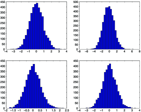
Figure 1: Standardized error distribution of $\bar{a}_{n}$ for $a=2$ (left) and $a=5$ (right) compound Poisson jumps with intensity $\lambda=1$ (top) and $\lambda=2$ (bottom).

Eventually, we find that the estimator performs well even for very short time horizons if the discretization is fine enough. This observation corresponds to the results of Theorem 4.2.12 in [18] that states that the discretization bias is of the order $\mathrm{O}(\Delta_{n})$.

5.2 Infinite intensity models

In Section 4, we have proved an asymptotic normality result for the discretized maximum likelihood estimator with jump filter (6) for models that involve a jump component of infinite activity. In this section, we simulate data from an Ornstein–Uhlenbeck model of the form (40) with $L=W+G$, where $W$ is a Wiener process with $E[W_{t}^{2}]=\sigma_{W}^{2}t$ and $G$ is a gamma process. Again, we consider an equidistant grid $t_{i}=i\Delta_{n}$ for $i=0,\ldots,n$. The gamma process has jumps of infinite activity, paths of finite variation and its Blumenthal–Getoor index is zero. The Lévy measure $\mu$ of $G$ has an explicit Lebesgue density given by

$$g(x)=cx^{-1}\mathrm{e}^{-\lambda x}\mathbf{1}_{\{x>0\}}\qquad\mbox{for $x\in\mathbb{R}$.}$$

The parameter $c>0$ controls the jump intensity and $\lambda>0$ the frequency of large jumps. It follows immediately from this density that $G$ is a subordinator. Exact simulation algorithms are known for increments of gamma processes and we use Johnk’s algorithm (cf. [5]).

Table 2 gives mean and standard deviation for different observation lengths and parameter values. The standard deviation scales approximately with $T^{-1/2}$ as expected from Theorem 4.6. In contrast to Table 1, we kept here $\Delta_{n}=0.0015$ fixed for all $n$. As in the finite intensity case we use the threshold exponent $\beta=0.3$ for the jump filter. We find that the value of $a$ has hardly any impact on the average number of increments that is filtered. When $a$ increases the number of filtered increments also increases slightly, since a greater variability of the drift might push increments with a relatively small jump over the threshold. Histograms of the standardized estimation error of $\bar{a}_{n}$ are given in Figure 2 for $a=2$ and $a=5$ and jumps from a gamma process.

Table 2: Results of 200 Monte Carlo simulations of $\bar{a}_{n}$ with $\Delta_{n}=0.0015$ and $\beta=0.3$ for gamma process jumps

		$a=2$			$a=5$
$c$	$T$	Mean	std dev	$\varnothing$ jumps detect	Mean	std dev	$\varnothing$ jumps detect
0.5	$1$	2.1	0.8	$2.4$	5.2	1.2	$2.2$
	$5$	2.0	0.4	$11.7$	5.0	0.6	$12.1$
	$7.5$	2.0	0.3	$17.7$	4.9	0.5	$17.8$
	$10$	2.0	0.3	$23.7$	5.0	0.4	$23.9$
	$20$	2.0	0.2	$47.2$	5.0	0.3	$47.6$
1	$1$	2.1	0.8	$1.6$	5.2	1.4	$1.8$
	$2.5$	2.1	0.6	$5.2$	5.1	1.1	$5.9$
	$5$	2.1	0.5	$8.4$	5.0	0.8	$8.6$
	$7.5$	2.0	0.5	$12.7$	5.0	0.7	$13.1$
	$10$	2.0	0.3	$17.2$	5.0	0.6	$17.1$

We conclude that the jump filtering approach performs well, also for models with infinite jump activity provided that the maximal observation distance is small.

5.3 Maximum likelihood vs. least squares estimation

In this section, we compare maximum likelihood and least squares estimation for the Ornstein–Uhlenbeck type process $X$ defined in (40). For continuously observed $X$, the least squares estimator for the drift parameter $a$ is given by

$$\hat{a}_{T}^{\mathrm{LS}}=-\frac{\int_{0}^{T}X_{s}\,\mathrm{d}X_{s}}{\int_{0}^{T}X_{s}^{2}\,\mathrm{d}s}.$$

For Gaussian Ornstein–Uhlenbeck processes, the least squares and the likelihood estimator $\hat{a}_{T}^{\mathrm{ML}}$ (4) coincide, since the continuous martingale part under $P^{a}$ equals the process itself. But when the driving process has jumps it follows from Theorem 4.2.10 in [18] that the asymptotic variances of both estimators differ by

$$\operatorname{AVAR}\bigl{(}\hat{a}_{T}^{\mathrm{LS}}\bigr{)}-\operatorname{AVAR}\bigl{(}\hat{a}_{T}^{\mathrm{ML}}\bigr{)}=E_{a}\bigl{[}X_{\infty}^{2}\bigr{]}^{-1}\int_{\mathbb{R}}x^{2}\mu(\mathrm{d}x)>0.$$

Hence, the least squares estimator is inefficient when jumps are present.

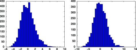
Figure 2: Error distribution of $\bar{a}_{n}$ for an Ornstein–Uhlenbeck process with $a=2$ (left) and $a=5$ (right), $\sigma_{W}=1$ and gamma process jumps.

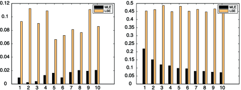
Figure 3: Bias (left) and standard deviation (right) of MLE and LSE for varying jump intensity.

Figure 3 compares the bias of the MLE and LSE for compound Poisson jumps with varying jump intensity. For each intensity the mean of 500 Monte Carlo simulations is given for an Ornstein–Uhlenbeck process with $\sigma_{W}=1$ and jumps with $N(0,2)$-distribution. The true parameter is $a=2$ and we find that the MLE has a significantly smaller bias than the LSE.

The standard deviation for both estimators is given in Figure 3 on the right. The jump intensity $\lambda$ of the compound Poisson part of $L$ varies between one and ten. In this model setup, the difference in asymptotic variance between MLE and LSE is given by

$$\operatorname{AVAR}\bigl{(}\hat{a}_{T}^{\mathrm{LS}}\bigr{)}-\operatorname{AVAR}\bigl{(}\hat{a}_{T}^{\mathrm{ML}}\bigr{)}=\frac{2a\sigma_{j}^{2}\lambda}{\sigma_{W}^{2}+\sigma_{j}^{2}\lambda}.$$

We observe that already for small jump intensities the MLE clearly outperforms the LSE. With growing intensity this efficiency gain becomes even more severe. For $\lambda=10$, the standard deviation is about five times larger for the least squares estimator.

This simulation example shows the significant gain in efficiency when we use a discretized likelihood estimator with approximation of the continuous part for drift estimation and underlines the importance of jump filtering for jump diffusion models.

References

• [1] {barticle}[mr] \bauthor\bsnmAït-Sahalia, \bfnmYacine\binitsY. &\bauthor\bsnmJacob, \bfnmJean\binitsJ. (\byear2007). \btitleVolatility estimators for discretely sampled Lévy processes. \bjournalAnn. Statist. \bvolume35 \bpages355–392. \biddoi=10.1214/009053606000001190, issn=0090-5364, mr=2332279 \bptokimsref\endbibitem
• [2] {barticle}[mr] \bauthor\bsnmAït-Sahalia, \bfnmYacine\binitsY. &\bauthor\bsnmJacod, \bfnmJean\binitsJ. (\byear2012). \btitleIdentifying the successive Blumenthal–Getoor indices of a discretely observed process. \bjournalAnn. Statist. \bvolume40 \bpages1430–1464. \biddoi=10.1214/12-AOS976, issn=0090-5364, mr=3015031 \bptokimsref\endbibitem
• [3] {barticle}[mr] \bauthor\bsnmBarndorff-Nielsen, \bfnmOle E.\binitsO.E. &\bauthor\bsnmShephard, \bfnmNeil\binitsN. (\byear2001). \btitleNon-Gaussian Ornstein–Uhlenbeck-based models and some of their uses in financial economics. \bjournalJ. R. Stat. Soc. Ser. B Stat. Methodol. \bvolume63 \bpages167–241. \biddoi=10.1111/1467-9868.00282, issn=1369-7412, mr=1841412 \bptokimsref\endbibitem
• [4] {barticle}[mr] \bauthor\bsnmBrockwell, \bfnmPeter J.\binitsP.J., \bauthor\bsnmDavis, \bfnmRichard A.\binitsR.A. &\bauthor\bsnmYang, \bfnmYu\binitsY. (\byear2007). \btitleEstimation for nonnegative Lévy-driven Ornstein–Uhlenbeck processes. \bjournalJ. Appl. Probab. \bvolume44 \bpages977–989. \biddoi=10.1239/jap/1197908818, issn=0021-9002, mr=2382939 \bptokimsref\endbibitem
• [5] {bbook}[mr] \bauthor\bsnmCont, \bfnmRama\binitsR. &\bauthor\bsnmTankov, \bfnmPeter\binitsP. (\byear2004). \btitleFinancial Modelling with Jump Processes. \bseriesChapman & Hall/CRC Financial Mathematics Series. \blocationBoca Raton, FL: \bpublisherChapman & Hall/CRC. \bidmr=2042661 \bptokimsref\endbibitem
• [6] {bbook}[mr] \bauthor\bsnmDudley, \bfnmR. M.\binitsR.M. (\byear2002). \btitleReal Analysis and Probability. \bseriesCambridge Studies in Advanced Mathematics \bvolume74. \blocationCambridge: \bpublisherCambridge Univ. Press. \bnoteRevised reprint of the 1989 original. \biddoi=10.1017/CBO9780511755347, mr=1932358 \bptokimsref\endbibitem
• [7] {barticle}[mr] \bauthor\bsnmFigueroa-López, \bfnmJosé E.\binitsJ.E. (\byear2008). \btitleSmall-time moment asymptotics for Lévy processes. \bjournalStatist. Probab. Lett. \bvolume78 \bpages3355–3365. \biddoi=10.1016/j.spl.2008.07.012, issn=0167-7152, mr=2479503 \bptokimsref\endbibitem
• [8] {barticle}[mr] \bauthor\bsnmHu, \bfnmYaozhong\binitsY. &\bauthor\bsnmLong, \bfnmHongwei\binitsH. (\byear2009). \btitleLeast squares estimator for Ornstein–Uhlenbeck processes driven by $\alpha$-stable motions. \bjournalStochastic Process. Appl. \bvolume119 \bpages2465–2480. \biddoi=10.1016/j.spa.2008.12.006, issn=0304-4149, mr=2532208 \bptokimsref\endbibitem
• [9] {bincollection}[auto:STB—2013/03/04—13:35:07] \bauthor\bsnmJacod, \bfnmJean\binitsJ. (\byear1985). \btitleGrossissements de filtration et processus d’Ornstein–Uhlenbeck généralisé. In \bbooktitleGrossissement de Filtrations: Exemples et Applications. Séminaire de Calcul Stochastique, Paris 1982/83. \bseriesLecture Notes in Math. \bvolume1118 \bpages36–44. \blocationBerlin: \bpublisherSpringer. \bptokimsref\endbibitem
• [10] {barticle}[mr] \bauthor\bsnmJacod, \bfnmJean\binitsJ. (\byear2007). \btitleAsymptotic properties of power variations of Lévy processes. \bjournalESAIM Probab. Stat. \bvolume11 \bpages173–196. \biddoi=10.1051/ps:2007013, issn=1292-8100, mr=2320815 \bptokimsref\endbibitem
• [11] {barticle}[mr] \bauthor\bsnmJahn, \bfnmPatrick\binitsP., \bauthor\bsnmBerg, \bfnmRune W.\binitsR.W., \bauthor\bsnmHounsgaard, \bfnmJørn\binitsJ. &\bauthor\bsnmDitlevsen, \bfnmSusanne\binitsS. (\byear2011). \btitleMotoneuron membrane potentials follow a time inhomogeneous jump diffusion process. \bjournalJ. Comput. Neurosci. \bvolume31 \bpages563–579. \biddoi=10.1007/s10827-011-0326-z, issn=0929-5313, mr=2864731 \bptokimsref\endbibitem
• [12] {barticle}[mr] \bauthor\bsnmJongbloed, \bfnmGeurt\binitsG. &\bauthor\bsnmvan der Meulen, \bfnmFrank H.\binitsF.H. (\byear2006). \btitleParametric estimation for subordinators and induced OU processes. \bjournalScand. J. Stat. \bvolume33 \bpages825–847. \biddoi=10.1111/j.1467-9469.2006.00498.x, issn=0303-6898, mr=2300918 \bptokimsref\endbibitem
• [13] {barticle}[mr] \bauthor\bsnmJongbloed, \bfnmG.\binitsG., \bauthor\bsnmvan der Meulen, \bfnmF. H.\binitsF.H. &\bauthor\bsnmvan der Vaart, \bfnmA. W.\binitsA.W. (\byear2005). \btitleNonparametric inference for Lévy-driven Ornstein–Uhlenbeck processes. \bjournalBernoulli \bvolume11 \bpages759–791. \biddoi=10.3150/bj/1130077593, issn=1350-7265, mr=2172840 \bptokimsref\endbibitem
• [14] {bmisc}[auto:STB—2013/03/04—13:35:07] \bauthor\bsnmKappus, \bfnmJohanna\binitsJ. (\byear2012). \bhowpublishedNonparametric adaptive estimation for discretely observed Lévy processes. Ph.D. thesis, Humboldt-Univ. zu Berlin. Available at http://edoc.hu-berlin.de/ docviews/abstract.php?lang=ger&id=39755. \bptokimsref\endbibitem
• [15] {bbook}[mr] \bauthor\bsnmKlenke, \bfnmAchim\binitsA. (\byear2008). \btitleProbability Theory: A Comprehensive Course. \bseriesUniversitext. \blocationLondon: \bpublisherSpringer. \biddoi=10.1007/978-1-84800-048-3, mr=2372119 \bptokimsref\endbibitem
• [16] {bbook}[mr] \bauthor\bsnmKüchler, \bfnmUwe\binitsU. &\bauthor\bsnmSørensen, \bfnmMichael\binitsM. (\byear1997). \btitleExponential Families of Stochastic Processes. \bseriesSpringer Series in Statistics. \blocationNew York: \bpublisherSpringer. \bidmr=1458891 \bptokimsref\endbibitem
• [17] {barticle}[mr] \bauthor\bsnmLánský, \bfnmP.\binitsP. &\bauthor\bsnmLánská, \bfnmV.\binitsV. (\byear1987). \btitleDiffusion approximation of the neuronal model with synaptic reversal potentials. \bjournalBiol. Cybernet. \bvolume56 \bpages19–26. \biddoi=10.1007/BF00333064, issn=0340-1200, mr=0885360 \bptokimsref\endbibitem
• [18] {bmisc}[auto:STB—2013/03/04—13:35:07] \bauthor\bsnmMai, \bfnmHilmar\binitsH. (\byear2012). \bhowpublishedDrift estimation for jump diffusions: Time-continuous and high-frequency observations. Ph.D. thesis, Humboldt-Univ. zu Berlin. Available at http://edoc. hu-berlin.de/docviews/abstract.php?id=39623. \bptokimsref\endbibitem
• [19] {barticle}[mr] \bauthor\bsnmMancini, \bfnmCecilia\binitsC. (\byear2009). \btitleNon-parametric threshold estimation for models with stochastic diffusion coefficient and jumps. \bjournalScand. J. Stat. \bvolume36 \bpages270–296. \biddoi=10.1111/j.1467-9469.2008.00622.x, issn=0303-6898, mr=2528985 \bptokimsref\endbibitem
• [20] {barticle}[mr] \bauthor\bsnmMancini, \bfnmCecilia\binitsC. (\byear2011). \btitleThe speed of convergence of the threshold estimator of integrated variance. \bjournalStochastic Process. Appl. \bvolume121 \bpages845–855. \biddoi=10.1016/j.spa.2010.12.001, issn=0304-4149, mr=2770909 \bptokimsref\endbibitem
• [21] {barticle}[mr] \bauthor\bsnmMasuda, \bfnmHiroki\binitsH. (\byear2007). \btitleErgodicity and exponential $\beta$-mixing bounds for multidimensional diffusions with jumps. \bjournalStochastic Process. Appl. \bvolume117 \bpages35–56. \biddoi=10.1016/j.spa.2006.04.010, issn=0304-4149, mr=2287102 \bptokimsref\endbibitem
• [22] {barticle}[mr] \bauthor\bsnmMasuda, \bfnmHiroki\binitsH. (\byear2010). \btitleApproximate self-weighted LAD estimation of discretely observed ergodic Ornstein–Uhlenbeck processes. \bjournalElectron. J. Stat. \bvolume4 \bpages525–565. \biddoi=10.1214/10-EJS565, issn=1935-7524, mr=2660532 \bptokimsref\endbibitem
• [23] {bbook}[mr] \bauthor\bsnmSato, \bfnmKen-iti\binitsK.-i. (\byear1999). \btitleLévy Processes and Infinitely Divisible Distributions. \bseriesCambridge Studies in Advanced Mathematics \bvolume68. \blocationCambridge: \bpublisherCambridge Univ. Press. \bidmr=1739520 \bptokimsref\endbibitem
• [24] {barticle}[mr] \bauthor\bsnmSato, \bfnmKen-iti\binitsK.-i. &\bauthor\bsnmYamazato, \bfnmMakoto\binitsM. (\byear1984). \btitleOperator-self-decomposable distributions as limit distributions of processes of Ornstein–Uhlenbeck type. \bjournalStochastic Process. Appl. \bvolume17 \bpages73–100. \biddoi=10.1016/0304-4149(84)90312-0, issn=0304-4149, mr=0738769 \bptokimsref\endbibitem
• [25] {barticle}[mr] \bauthor\bsnmShimizu, \bfnmYasutaka\binitsY. (\byear2006). \btitle$M$-estimation for discretely observed ergodic diffusion processes with infinitely many jumps. \bjournalStat. Inference Stoch. Process. \bvolume9 \bpages179–225. \biddoi=10.1007/s11203-005-8113-y, issn=1387-0874, mr=2249182 \bptokimsref\endbibitem
• [26] {bmisc}[auto:STB—2013/03/04—13:35:07] \bauthor\bsnmSørensen, \bfnmMichael\binitsM. (\byear1991). \bhowpublishedLikelihood methods for diffusions with jumps. In Statistical Inference in Stochastic Processes. New York: Dekker. \bptokimsref\endbibitem