Rare semileptonic $B\to K^{*}\ell^{+}\ell^{-}$ decays in RS_c model

Abstract

Recent LHCb measurements show small discrepancies with respect to the Standard Model (SM) predictions in selected angular distributions of the mode $B^{0}\to K^{*0}\mu^{+}\mu^{-}$. The possibility of explaining such tensions within theories beyond the SM crucially depends on the size of the deviations of the Wilson coefficients of the effective Hamiltonian for this mode, in comparison to their SM values. We analyse this issue in the framework of the Randall Sundrum model with custodial protection (RS_c); in our study we also consider the mode with $\tau$ leptons in the final state. We discuss the small deviations of RS_c results from SM ones, found scanning the parameter space of the model.

I Introduction

Despite the phenomenological success of the Standard Model (SM), there are hints that the paths to new physics are open, and that they pass across the flavour sector. Joint efforts at the $B$ factories and at the hadron colliders have provided us with data of unprecedented precision in this sector, so that we are now sensitive to small effects in theoretical calculations that are essential in the comparison with the measurements. Moreover, the large sample of collected data has further enriched the experimental scenario, and information is now available on particular processes forseen as the most promising ones to unveil deviations from SM. Among those, a prominent role is played by the measurement of the rare $B_{s,d}\to\mu^{+}\mu^{-}$ branching fractions Aaij:2013aka ; Chatrchyan:2013bka :

$${\bar{\cal B}}(B_{s}\to\mu^{+}\mu^{-}) = (2.9\pm 0.7)\times 10^{-9}\,\,\,\,,$$

$${\cal B}(B_{d}\to\mu^{+}\mu^{-}) = (3.6\pm^{1.6}_{1.4})\times 10^{-10}\,\,\,\,\,\,,$$ (1)

where the symbol $\bar{\cal B}$, in the case of $B_{s}$, indicates that the effect of width difference in the $B_{s}-\bar{B}_{s}$ system is taken into account Dunietz:2000cr . The corresponding SM predictions are Bobeth:2013uxa :

$${\bar{\cal B}}(B_{s}\to\mu^{+}\mu^{-})_{SM} = (3.65\pm 0.23)\times 10^{-9}\,\,\,\,,$$

$${\cal B}(B_{d}\to\mu^{+}\mu^{-})_{SM} = (1.06\pm 0.09)\times 10^{-10}\,\,,$$ (2)

including the errors on the meson lifetimes, on the top quark mass and $\alpha_{s}$, on the values of the CKM matrix elements and on the decay constants $f_{B_{s,d}}$. The comparison between (1) and (2) shows the existing agreement in the case of $B_{s}$, which excludes large contributions from new scalar or pseudoscalar particles; in the case of $B_{d}\to\mu^{+}\mu^{-}$ the SM prediction undershoots the measurement, but the uncertainties are too large to draw conclusions.

Another process recognized as particularly sensitive to new physics effects is the rare semileptonic $B\to K^{*}\mu^{+}\mu^{-}$ decay, mainly due to the numerous observables that can be studied to disentangle additional new particle contributions in this loop-driven transition. Several measurements were already available from $B$ factories, such as the branching fraction, the forward-backward lepton asymmetry and the $K^{*}$ longitudinal polarization fraction in few bins of the squared momentum transferred to the lepton pair, $q^{2}$. Analyses at LHC have improved the scenario, enlarging the set of the measured observables Aaij:2011aa ; Aaij:2013iag ; Aaij:2013qta ; Usanova:2013osa ; Chatrchyan:2013cda . A recent LHCb investigation has reported a set of 24 measurements, disclosing a problematic effect in particular observables, as described below. This has prompted several discussions aimed at explaining the discrepancy and at understanding in which direction new physics effects should prominently appear.

In this work, we study the $B\to K^{*}\ell^{+}\ell^{-}$ mode in the framework of the Randall-Sundrum model, a new physics framework justified by several theoretical considerations RandallSundrum . In this model, the space-time is supposed to be five-dimensional with warped metric, so that in its 4D reduction new particles appear that are either Kaluza-Klein excitation of SM particles, or new ones having no SM counterparts. Additional contributions to the considered rare mode are therefore produced, and we discuss whether they can explain the observed pattern of measurements, preserving the agreement of the computed $\bar{\cal B}(B_{s}\to\mu^{+}\mu^{-})$ with data. In our analysis we consider both the cases $\ell=\mu$ (and $e$) and $\ell=\tau$. The reason is that tensions with SM predictions have also been found in the branching fractions of semileptonic $B$ decays with a $\tau$ lepton in the final state Lees:2012xj ; taus . It is therefore interesting to work out predictions for other decay modes involving the $\tau$ lepton.

Several studies of $B$ decays in the RS framework exist in the literature burdman ; agashe ; moreau ; neubertRS ; buras1 ; buras2 ; Albrecht:2009xr ; buras4 ; Blanke:2012tv . An important issue concerns the mass scale of the lowest Kaluza-Klein excitations $M_{KK}$ that is compatible with existing data on flavour observables. In this respect the main problem (the so-called flavour problem in RS) is represented by the parameter $\epsilon_{K}$ describing indirect CP violation in the Kaon sector. Agreement with data for this parameter would require large $M_{KK}$, of the order of tens TeV. In order to allow mass values in a range accessible to the LHC without a strong fine tuning to predict $\epsilon_{K}$ in its experimental range, several solutions have been proposed, namely an extended gauge group for strong interactions Bauer:2011ah or additional symmetries Santiago:2008vq ; Fitzpatrick:2007sa . In the framework of the so-called custodial RS_c model, it has been shown that it is possible to have $M_{KK}={\cal O}(1\,\,{\rm TeV})$ without requiring too much fine tuning to reproduce $\epsilon_{K}$ in the measured range buras1 ; buras2 ; Albrecht:2009xr ; buras4 . For such low mass scales, sizeable deviations from SM predictions in $\Delta F=2$ observables are possible, with the main role in particle-antiparticle mixing diagrams coming from the first KK excitation of the gluon, at least in the Kaon sector, while for $B_{d,s}$ mixing also KK excitations of the electroweak gauge bosons play a role, and in particular the new gauge boson $Z_{H}$, that we introduce below, is important burdman ; buras1 . On the other hand, it has been shown that the effects are less pronounced in the inclusive $\Delta F=1$ $B$ decays, at odds with the Kaon $\Delta F=1$ transitions buras2 . In both sectors, the main new contribution comes from the modification of $Z$ couplings to right-handed down-type quarks, since the left-handed ones are protected by the custodial symmetry.

In buras2 the inclusive $b\to s\ell^{+}\ell^{-}$ decay modes were considered neglecting the modifications of the coefficients of the dipole operators in the relevant effective Hamiltonian which appear at loop level. The changes of such coefficients in the RS framework have been computed to study the inclusive $B\to X_{s}\gamma$ decay mode Blanke:2012tv . Our analysis is complementary to those performed in buras2 ; Blanke:2012tv in several respects, since for example we study the exclusive mode $B\to K^{*}\ell^{+}\ell^{-}$, which requires a set of hadronic form factors. Furthermore, we provide a calculation of the coefficients of the dipole operators using a different technique with respect to that carried out in Blanke:2012tv , which more consistently matches with the other parts of the calculation. A prime attention is paid to the bounds provided to the parameter space of the model by the present experimental knowledge, in particular of the CKM mixing matrix. Moreover, we study in details the modes with $\tau$ leptons, and the sensitivity of their additional observables to this new physics scenario.

The plan of the paper is the following. In Sec. II we fix our notations for the effective Hamiltonian governing the process $B\to K^{*}\ell^{+}\ell^{-}$, and collect the definitions required in the subsequent discussion. In Sec. III we describe the main features of the RS_c model, in particular the particle content and the couplings relevant for our study. The numerical analysis follows in Sec. V and VI, where we investigate all the measured observables in $B\to K^{*}\mu^{+}\mu^{-}$ and present a set of predictions for the mode with $\tau$ leptons. Concluding remarks can be found in Sec. VII. In the Appendices we collect several technical details, in particular those relevant for our calculation of the Wilson coefficients $\Delta C_{7,8}^{(\prime)}$: the profiles of various KK states, the couplings of neutral bosons to fermions, and the different contributions to the Wilson coefficients.

II General features of the $B\to K^{*}\ell^{+}\ell^{-}$ decay mode

The effective $\Delta B=-1$, $\Delta S=1$ Hamiltonian governing the rare transition $b\to s\ell^{+}\ell^{-}$ can be written as

$$H^{eff} = -\,4\,{G_{F}\over\sqrt{2}}V_{tb}V_{ts}^{*}\,\Big{\{}C_{1}O_{1}+C_{2}O_{2}$$ (3)

$$+ \sum_{i=3,..,6}C_{i}O_{i}+\sum_{i=7,..,10,P,S}\left[C_{i}O_{i}+C_{i}^{\prime}O_{i}^{\prime}\right]\Big{\}}\,,\,\,\,\,\,\,$$

where $G_{F}$ is the Fermi constant and $V_{ij}$ are elements of the Cabibbo-Kobayashi-Maskawa mixing matrix. We neglect doubly Cabibbo suppressed terms proportional to $V_{ub}V_{us}^{*}$. $O_{1}$ and $O_{2}$ are current-current operators, and $O_{i}$ $(i=3,\dots,6)$ are QCD penguins; they have a minor impact on the modes we are considering, therefore we neglect them and refer to Buchalla:1995vs for details about their structure. Among the remaining operators, the primed ones have opposite chirality with respect to the unprimed. Only the unprimed ones, for $i=7,\dots 10$, are present in the SM; the scalar $O_{S}$ and pseudoscalar $O_{P}$ operators, although present in SM, are highly suppressed. Therefore, the operators considered in our analysis are

• Magnetic penguin operators:

  $$O_{7} = {e\over 16\pi^{2}}m_{b}({\bar{s}}_{L\alpha}\sigma^{\mu\nu}b_{R\alpha})F_{\mu\nu}$$

  $$O_{7}^{\prime} = \frac{e}{16\pi^{2}}m_{b}({\bar{s}}_{R\alpha}\sigma^{\mu\nu}b_{L\alpha})F_{\mu\nu}$$

  $$O_{8} = {g_{s}\over 16\pi^{2}}m_{b}\Big{[}{\bar{s}}_{L\alpha}\sigma^{\mu\nu}\Big{(}{\lambda^{a}\over 2}\Big{)}_{\alpha\beta}b_{R\beta}\Big{]}\;G^{a}_{\mu\nu}$$ (4)

  $$O_{8}^{\prime} = {g_{s}\over 16\pi^{2}}m_{b}\Big{[}{\bar{s}}_{R\alpha}\sigma^{\mu\nu}\Big{(}{\lambda^{a}\over 2}\Big{)}_{\alpha\beta}b_{L\beta}\Big{]}\;G^{a}_{\mu\nu}\,\,,$$

• Semileptonic electroweak penguin operators:

  $$O_{9} = {e^{2}\over 16\pi^{2}}({\bar{s}}_{L\alpha}\gamma^{\mu}b_{L\alpha})\;{\bar{\ell}}\gamma_{\mu}\ell$$

  $$O_{9}^{\prime} = {e^{2}\over 16\pi^{2}}({\bar{s}}_{R\alpha}\gamma^{\mu}b_{R\alpha})\;{\bar{\ell}}\gamma_{\mu}\ell$$

  $$O_{10} = {e^{2}\over 16\pi^{2}}({\bar{s}}_{L\alpha}\gamma^{\mu}b_{L\alpha})\;{\bar{\ell}}\gamma_{\mu}\gamma_{5}\ell$$ (5)

  $$O_{10}^{\prime} = {e^{2}\over 16\pi^{2}}({\bar{s}}_{R\alpha}\gamma^{\mu}b_{R\alpha})\;{\bar{\ell}}\gamma_{\mu}\gamma_{5}\ell\,\,.$$

In (4-5) $\alpha$ and $\beta$ are colour indices, $\lambda^{a}$ the Gell-Mann matrices, and $\displaystyle b_{R,L}={1\pm\gamma_{5}\over 2}b$. $F_{\mu\nu}$ and $G^{a}_{\mu\nu}$ denote the electromagnetic and the gluonic field strength tensors, respectively, and $e$ and $g_{s}$ are the electromagnetic and the strong coupling constants. $m_{b}$ is the $b$ quark mass, while the operators proportional to the strange quark mass $m_{s}$ are neglected.

Considering the subsequent resonant $K^{*}\to K\pi$ decay, the $B\to K^{*}(\to K\pi)\ell^{+}\ell^{-}$ fully differential decay width can be written as follows:

$$\frac{d^{4}\Gamma(B\to K^{*}[\to K\pi]\ell^{+}\ell^{-})}{dq^{2}d\cos\theta_{\ell}d\cos\theta_{K}d\phi}=\frac{9}{32\pi}I(q^{2},\theta_{\ell},\theta_{K},\phi)\,\,\,,$$ (6)

where

$$I(q^{2},\theta_{\ell},\theta_{K},\phi) = I_{1}^{s}\sin^{2}\theta_{K}+I_{1}^{c}\cos^{2}\theta_{K}$$ (7)

$$+ (I_{2}^{s}\sin^{2}\theta_{K}+I_{2}^{c}\cos^{2}\theta_{K})\cos 2\theta_{\ell}$$

$$+ I_{3}\sin^{2}\theta_{K}\sin^{2}\theta_{\ell}\cos 2\phi$$

$$+ I_{4}\sin 2\theta_{K}\sin 2\theta_{\ell}\cos\phi$$

$$+ I_{5}\sin 2\theta_{K}\sin\theta_{\ell}\cos\phi$$

$$+ (I_{6}^{s}\sin^{2}\theta_{K}+I_{6}^{c}\cos^{2}\theta_{K})\cos\theta_{\ell}$$

$$+ I_{7}\sin 2\theta_{K}\sin\theta_{\ell}\sin\phi$$

$$+ I_{8}\sin 2\theta_{K}\sin 2\theta_{\ell}\sin\phi$$

$$+ I_{9}\sin^{2}\theta_{K}\sin^{2}\theta_{\ell}\sin 2\phi\,.$$

In the previous equations, $q^{2}$ is the dilepton invariant mass; $\theta_{K}$ is the angle between the Kaon direction and the direction opposite to the $B$ meson one in the $K^{*}$ rest frame; $\theta_{\ell}$ is the angle between the charged lepton direction and the direction opposite to that the $B$ meson in the lepton pair rest frame; finally, $\phi$ is the angle between the plane containing the lepton pair and the plane containing the $K^{*}$ decay products, i.e. $K$ and $\pi$ Faessler:2002ut ; Altmannshofer:2008dz . In the case of the CP conjugated mode, the $\bar{B}$ meson decay, one defines analogous functions $\bar{I}$ in which all the weak phases are conjugated. The fully differential decay width $d\bar{\Gamma}$ can be written in analogy to (6), with the function $I$ replaced by $\bar{I}$ which is obtained from (7) by the rule Altmannshofer:2008dz :

$$I_{1,2,3,4,7} \to {\bar{I}}_{1,2,3,4,7}$$

$$I_{5,6,8,9} \to -{\bar{I}}_{5,6,8,9}\,\,\,.$$ (8)

All the functions $I_{i}(\bar{I}_{i})$ can be written in terms of eight transversity amplitudes, which in turn are functions of the $B\to K^{*}$ form factors. We adopt the following parametrization for the $B\to K^{*}$ matrix elements:

$$<K^{*}(p^{\prime},\epsilon)|{\bar{s}}\gamma_{\mu}(1-\gamma_{5})b|B(p)>=\hskip 99.58464pt$$

$$\epsilon_{\mu\nu\alpha\beta}\epsilon^{*\nu}p^{\alpha}p^{\prime\beta}{2V(q^{2})\over M_{B}+M_{K^{*}}}\hskip 14.22636pt$$

$$-i\left[\epsilon^{*}_{\mu}(M_{B}+M_{K^{*}})A_{1}(q^{2})-(\epsilon^{*}\cdot q)(p+p^{\prime})_{\mu}{A_{2}(q^{2})\over M_{B}+M_{K^{*}}}\right.$$

$$-\left.(\epsilon^{*}\cdot q){2M_{K^{*}}\over q^{2}}\big{(}A_{3}(q^{2})-A_{0}(q^{2})\big{)}q_{\mu}\right]\,\,,\,\,\,\hskip 14.22636pt$$ (9)

$$<K^{*}(p^{\prime},\epsilon)|{\bar{s}}\sigma_{\mu\nu}q^{\nu}{(1+\gamma_{5})\over 2}b|B(p)>=\hskip 56.9055pt$$

$$i\epsilon_{\mu\nu\alpha\beta}\epsilon^{*\nu}p^{\alpha}p^{\prime\beta}\;2\;T_{1}(q^{2})\hskip 14.22636pt$$

$$+\Big{[}\epsilon^{*}_{\mu}(M_{B}^{2}-M^{2}_{K^{*}})-(\epsilon^{*}\cdot q)(p+p^{\prime})_{\mu}\Big{]}\;T_{2}(q^{2})\hskip 14.22636pt$$

$$+(\epsilon^{*}\cdot q)\left[q_{\mu}-{q^{2}\over M_{B}^{2}-M^{2}_{K^{*}}}(p+p^{\prime})_{\mu}\right]\;T_{3}(q^{2})\,,\,\,\,\,\,\,$$ (10)

where $\epsilon$ is the $K^{*}$ polarization vector. The various form factors are not all independent; $A_{3}$ can be written as

$$A_{3}(q^{2})={M_{B}+M_{K^{*}}\over 2M_{K^{*}}}A_{1}(q^{2})-{M_{B}-M_{K^{*}}\over 2M_{K^{*}}}A_{2}(q^{2})$$ (11)

with $A_{3}(0)=A_{0}(0)$; moreover, the identity $\displaystyle\sigma_{\mu\nu}\gamma_{5}=-{i\over 2}\epsilon_{\mu\nu\alpha\beta}\sigma^{\alpha\beta}$ (with $\epsilon_{0123}=+1$) implies $T_{1}(0)=T_{2}(0)$. Using these definitions, the transversity amplitudes entering in the $I_{i}$ structures, and the $I_{i}$ functions themselves, can be found in Ref. Altmannshofer:2008dz (their Eqs. (3.28)-(3.45)), with the only change that the three $T_{i}$ form factors in that paper have to be divided by a factor of $2$ to match our definition in Eq.(10).

From the functions $I_{i}(q^{2})$ and $\bar{I}_{i}(q^{2})$, CP conserving quantities ($S_{i}$) and CP asymmetries ($A_{i}$) can be built:

$$S_{i} = \frac{I_{i}+\bar{I}_{i}}{\frac{d\Gamma}{dq^{2}}+\frac{d\bar{\Gamma}}{dq^{2}}}\,\,,$$ (12)

$$A_{i} = \frac{I_{i}-\bar{I}_{i}}{\frac{d\Gamma}{dq^{2}}+\frac{d\bar{\Gamma}}{dq^{2}}}\,\,.$$ (13)

Starting from these quantities, several observables can be introduced. In particular, we consider

• the lepton forward-backward (FB) asymmetry: $A_{FB}=-\frac{3}{8}(2S_{6}^{s}+S_{6}^{c})$;

• the longitudinal $K^{*}$ polarization fraction: $F_{L}=-S_{2}^{c}$;

• binned observables $S_{i}$ , with their numerators and denominators separately integrated over $q^{2}$ bins of the kind $[q^{2}_{1},q^{2}_{2}]$: $<S_{i}>_{[q^{2}_{1},q^{2}_{2}]}$.

These are the main observables analyzed in the present investigation, that will be compared to the experimental results.

Of great interest is the lepton FB asymmetry. The first analyses by BaBar, Belle and CDF Collaborations seemed to contradict the SM expectation for the sign of $A_{FB}(q^{2})$ in the low $q^{2}$ region: $q^{2}\in[1-6]$ GeV² Aubert:2008bi ; Wei:2009zv ; Aaltonen:2011ja . The presently available improved analysis by LHCb shows agreement with SM Aaij:2011aa , as we discuss in more details below. On general grounds, $A_{FB}$ might or not have a zero in the kinematically accessible $q^{2}$ range. The position of such a zero, in terms of the $B\to K^{*}$ form factors and of the Wilson coefficients in the effective Hamiltonian (3), is given by the value of $q^{2}$ for which the equation holds:

$${\rm Re}\Bigg{\{}\frac{2m_{b}}{q^{2}}\left[(M_{B}+M_{K^{*}})\frac{T_{1}(q^{2})}{V(q^{2})}(C_{7}+C_{7}^{\prime})(C_{10}-C_{10}^{\prime})^{*}\right.$$

$$\left.+(M_{B}-M_{K^{*}})\frac{T_{2}(q^{2})}{A_{1}(q^{2})}(C_{7}-C_{7}^{\prime})(C_{10}+\,C_{10}^{\prime})^{*}\right]$$

$$+C_{9}\,C_{10}^{*}-C_{9}^{\prime}C_{10}^{\prime*}\Bigg{\}}=0\,\,\,\,\,.$$

(14)

In SM this equation becomes:

$${\rm Re}\left\{\frac{2m_{b}}{q^{2}}\Big{[}\Big{(}(M_{B}+M_{K^{*}})\frac{T_{1}(q^{2})}{V(q^{2})}\right.\hskip 85.35826pt$$

$$\left.+(M_{B}-M_{K^{*}})\frac{T_{2}(q^{2})}{A_{1}(q^{2})}\Big{)}C_{7}\,C_{10}^{*}\Big{]}+C_{9}\,C_{10}^{*}\right\}=0\,\,.\,\,\,\,\,\,\,\,\,$$ (15)

In the large energy limit of $K^{*}$ and in the heavy quark limit the $q^{2}$ dependence of the form factor ratios in (14), (15) cancels out, and $T_{1}/V=M_{B}/(M_{B}+M_{K^{*}})$, $T_{2}/A_{1}=(M_{B}+M_{K^{*}})/M_{B}$ (modulo radiative corrections); hence, the position of the zero of $A_{FB}$ is, to a large extent, a quantity which only depends on the structure of the interactions, i.e. it is independent of the form factors, and at NLO for the Wilson coefficients it is given by $q_{0}^{2}|_{SM}=4.39\pm^{0.38}_{0.35}$ GeV² Beneke:2001at . This value must be compared with the LHCb determination: $q_{0}^{2}|_{LHCb}=4.9\pm 0.9$ GeV² Aaij:2013iag .

Results that have raised interest are those reported by the LHCb Collaboration Aaij:2013qta , with the measurement of the observables DescotesGenon:2012zf

$$P^{\prime}_{i=4,5,6,8}=\frac{S_{i=4,5,7,8}}{\sqrt{F_{L}(1-F_{L})}}\,\,$$ (16)

related to $F_{L}$ and $S_{i}$ defined above. The measurement is carried out in $6$ bins of $q^{2}$ for each one of the four observables in (16): a discrepancy is found in the case of $P_{5}^{\prime}$ in the third $q^{2}$ bin, where the datum is significantly lower than the SM prediction, as we show below. A small deviation is also found in $P_{4}^{\prime}$ for another value of $q^{2}$. Efforts have been devoted to identify the kind of new physics effects which may explain the full set of data without altering the observables in agreement with SM predictions. The general idea is to try to understand which one of the Wilson coefficients (and how many of them) should be modified (increased/suppressed), including those not present in SM, to reproduce the data Descotes-Genon:2013wba ; Altmannshofer:2013foa ; Beaujean:2013soa .

In the following we do not adopt the phenomenological approach of looking separately at the various Wilson coefficients, but rather we make use of a specific new physics scenario, the custodially protected Randall-Sundrum model, in which the weak effective Hamiltonian emerges from a well defined theory of elementary interactions. The resulting Wilson coefficients are therefore correlated, and such a correlation has precise phenomenological consequences to be considered in the various observables, namely those in (16). Moreover, motivated by the experimental results of semileptonic and leptonic $B$ decays to $\tau$ leptons, we also study observables for the case of massive final leptons, namely the $\tau$ polarization asymmetries.

To define polarization asymmetries, let us consider the spin vector $s$ of the $\tau^{-}$ lepton having momentum $k_{1}$, with $s^{2}=-1$ and $k_{1}\cdot s=0$. In the $\tau^{-}$ rest frame three orthogonal unit vectors can be defined, $\vec{e}_{L}$, $\vec{e}_{N}$ and $\vec{e}_{T}$, corresponding to the longitudinal $s_{L}$, normal $s_{N}$ and transverse $s_{T}$ polarization vectors:

$$s_{L} = (0,\vec{e}_{L})=\left(0,{\vec{k}_{1}\over|\vec{k}_{1}|}\right)$$

$$s_{N} = (0,\vec{e}_{N})=\left(0,{\vec{p}^{\prime}\times\vec{k}_{1}\over|\vec{p}^{\prime}\times\vec{k}_{1}|}\right)$$ (17)

$$s_{T} = (0,\vec{e}_{T})=(0,\vec{e}_{N}\times\vec{e}_{L})\,\,\,.$$

In Eq.(17) $\vec{p}^{\prime}$ and $\vec{k}_{1}$ are the $K^{*}$ and $\tau^{-}$ three-momenta in the rest frame of the lepton pair. Choosing the $z$-axis directed as the $\tau^{-}$ momentum in the lepton pair rest frame we have $k_{1}=(E_{1},0,0,|\vec{k}_{1}|)$, and boosting the spin vectors $s$ in (17) in the rest frame of the lepton pair, the normal and transverse polarization vectors $s_{N}$, $s_{T}$ remain unchanged, $s_{N}=(0,1,0,0)$ and $s_{T}=(0,0,-1,0)$, while the longitudinal polarization vector becomes:

$$s_{L}={1\over m_{\tau}}(|\vec{k}_{1}|,0,0,E_{1})\,\,\,.$$ (18)

For each value of the squared momentum transfered to the lepton pair, $q^{2}$, the polarization asymmetry for the negatively charged $\tau^{-}$ lepton can be defined as:

$${\cal A}_{A}(q^{2})={\displaystyle{d\Gamma\over dq^{2}}(s_{A})-{d\Gamma\over dq^{2}}(-s_{A})\over{\displaystyle{d\Gamma\over dq^{2}}(s_{A})+{d\Gamma\over dq^{2}}(-s_{A})}}\,\,\,,$$ (19)

with $A=L$, $T$ and $N$. These quantities have been analysed in the SM (e.g. in Kruger:1996cv ; Colangelo:2006gv and in the references therein). In particular, in Ref.Colangelo:2006gv it has been pointed out that the $\tau$ polarization asymmetries are also form factor independent quantities in the $q^{2}$ region where the large energy limit can be applied. These results can be generalized including the new primed operators considered here. In particular, one can exploit the expressions in Colangelo:2006gv for the observables in $B\to K^{*}\tau^{+}\tau^{-}$ with the substitutions

$$C_{7}\,T_{1} \to (C_{7}+C_{7}^{\prime})\,T_{1}$$

$$C_{7}\,T_{2,3} \to (C_{7}-C_{7}^{\prime})\,T_{2,3}$$

$$C_{9}\,V \to (C_{9}+C_{9}^{\prime})\,V$$

$$C_{10}\,V \to (C_{10}+C_{10}^{\prime})\,V$$ (20)

$$C_{9}\,A_{1,2} \to (C_{9}-C_{9}^{\prime})A_{1,2}$$

$$C_{10}\,A_{1,2,0} \to (C_{10}-C_{10}^{\prime})\,A_{1,2,0}\,\,.$$

We adopt these prescriptions in the following discussion.

III Randall-Sundrum model with custodial protection

In this Section we describe the main features of the Randall-Sundrum (RS) model RandallSundrum , a theoretical framework constructed with the motivation, among others, represented by the possibility of solving the hierarchy problem and of explaining the observed hierarchies in the fermion masses and mixing angles. The model is defined in a five dimensional space-time manifold with coordinates $(x,y)$ ($x$ the ordinary Minkowskian coordinates) and metric

$$ds^{2} = e^{-2ky}\eta_{\mu\nu}dx^{\mu}dx^{\nu}-dy^{2}\,\,\,,$$

$$\eta_{\mu\nu} = diag(+1,-1,-1,-1)\,\,\,.$$ (21)

The scale parameter $k$ is chosen $k\simeq{\cal O}(M_{Planck})$ to address the hierarchy problem; we set it to $k=10^{19}$ GeV. The (fifth) coordinate $y$ varies in a range between two branes, $0\leq y\leq L$; $y=0$ corresponds to the so-called UV brane, $y=L$ to the IR one.

Several variants of the model have been proposed, each one adding new features to those of the original model. Here, we consider the scenario in which the SM gauge symmetry group is enlarged to the gauge group

$$SU(3)_{c}\times SU(2)_{L}\times SU(2)_{R}\times U(1)_{X}\times P_{L,R}\,\,$$ (22)

which, together with the metric, defines the Randall-Sundrum model with custodial protection RS_c contino ; carena ; cacciapaglia . The custodial protection is realized imposing the discrete $Z_{2}$ $P_{L,R}$ symmetry, which implies a mirror action of the two $SU(2)_{L,R}$ groups, preventing large $Z$ couplings to left-handed fermions that would be incompatible with experiment. Furthermore, this variant has been proven to be consistent with electroweak precision observables for masses of the lightest Kaluza-Klein excitations of the order of a few TeV Contino:2006qr ; Carena:2007ua , in the reach of the LHC.

Two symmetry breakings occur: first, the gauge group (22) is broken to the SM gauge group imposing suitable boundary conditions (BC) on the UV brane. Afterwards, the spontaneous symmetry breaking occurs, which is Higgs-driven as in SM. All the SM fields are allowed to propagate in the bulk, except for the Higgs field which is localized close to the IR brane. Here, we consider the case of a Higgs boson completely localized at $y=L$.

The extension of the SM leads to the presence of new particles, as a consequence of the requirements/assumptions listed below.

• The two $SU(2)$ groups require a larger number of gauge bosons. Those corresponding to $SU(2)_{L}$ are $W_{L}^{a,\mu}$ ($a=1,2,3$), while $W_{R}^{a,\mu}$ correspond to $SU(2)_{R}$. The gauge conditions $W_{L,R}^{a,5}=0$ and $\partial_{\mu}W_{L,R}^{a,\mu}=0$ are chosen, as well as for all the other gauge bosons. The $P_{L,R}$ symmetry imposes the equality $g_{L}=g_{R}=g$ for the $SU(2)_{L,R}$ gauge couplings.

  The number of remaining gauge bosons is the same as in SM. In particular, the eight gauge fields corresponding to $SU(3)_{c}$ are still identified with the gluons, while the $U(1)_{X}$ gauge field is denoted as $X_{\mu}$, with coupling $g_{X}$. The 5D couplings are dimensionful: the relations to their 4D counterparts are $g^{4D}={g^{5D}}/{\sqrt{L}}$. We shall describe below the mixing pattern among the various gauge fields.

• Fitting matter fields in suitable representations of the group (22) leads to new fermions, as discussed in the following.

• The presence of a compact fifth dimension implies the existence of a tower of Kaluza-Klein (KK) excitations for all particles. As generically done in extra-dimensional models, the boundary conditions help to distinguish particles having a SM correspondent from those without SM partners, by requiring the existence or not of a zero mode in the KK mode expansion of a given field. Two choices for BC are considered: Neumann BC on both branes (++), or Dirichlet BC on the UV brane and Neumann BC on the IR one (-+). Only fields with (++) BC have a zero mode which can be identified with a SM particle.

For each one of the fields listed above we perform a KK decomposition of the generic form:

$$F(x,y)=\frac{1}{\sqrt{L}}\sum_{k}F^{(k)}(x)f^{(k)}(y)\,\,,$$ (23)

referring to the functions $f^{(k)}(y)$ (specific for each field $F$) as the 5D field profiles, while $F^{(k)}(x)$ are the corresponding effective 4D fields. Then, we consider the 5D Lagrangian densities for the various fields, and solve the resulting 5D equations of motion to obtain the various profiles. Following the strategy outlined in Albrecht:2009xr , this can be done before the EWSB. After such a symmetry breaking takes place, one can treat the ratio $v/M_{KK}$ of the Higgs vacuum expectation value (vev) $v$ and the mass of the lowest KK mode $M_{KK}$ as a perturbation. The effective 4D Lagrangian is obtained after integration over $y$, and the Feynman rules of the model are worked out neglecting terms of ${\cal O}(v^{2}/M_{KK}^{2})$ or higher. On the same footing, the mixing occurring between SM fermions and higher KK fermion modes can be neglected, since it leads to ${\cal O}(v^{2}/M_{KK}^{2})$ modifications of the relevant couplings.

As for gauge bosons, we consider KK modes up to the first excitation (1-mode). Indeed, as observed in buras1 , the model becomes non perturbative already for scales corresponding to the first few KK modes, so that including the whole tower of excitations would lead to unreliable results.

Let us now examine the various sectors of the model, stressing the most relevant features for our analysis.

III.1 Higgs sector

After the gauge group (22) has undergone the breaking to the SM $SU(3)_{c}\times SU(2)_{L}\times U(1)_{Y}$, the electroweak symmetry breaking takes place. A Higgs field $H(x,y)$ is introduced, which transforms as a bidoublet under $SU(2)_{L}\times SU(2)_{R}$ and as a singlet under $U(1)_{X}$. This field contains two charged and two neutral components:

$$H(x,y)=\left(\begin{array}[]{cc}\frac{\pi^{+}}{\sqrt{2}}&-\frac{h^{0}-i\pi^{0}}{2}\\ \frac{h^{0}+i\pi^{0}}{2}&\frac{\pi^{-}}{\sqrt{2}}\end{array}\right)\,\,\,.$$

Performing the KK decomposition, one writes

$$H(x,y)=\frac{1}{\sqrt{L}}\sum_{k}H^{(k)}(x)h^{(k)}(y)\,\,.$$ (24)

For the Higgs localized on the IR brane the choice

$$h(y)\equiv h^{(0)}(y)\simeq e^{kL}\delta(y-L)$$ (25)

is done. As for the components depending on the 4D coordinates, one chooses that only the neutral field $h^{0}$ has a non vanishing vacuum expectation value coinciding with the SM Higgs vev $v=246.22$ GeV. The 5D action involving the Higgs field reads:

$$S_{Higgs}=\hskip 199.16928pt$$

$$\int d^{4}x\int_{0}^{L}dy\sqrt{G}\,{\rm Tr}\Big{[}[D_{M}H(x,y)]^{\dagger}[D^{M}H(x,y)]-V(H)\Big{]}\,\,,$$

with $\sqrt{G}=det[g_{MN}]=e^{-4ky}$, $g_{MN}$ being the 5D metric tensor and $M,N=0,1,2,3,5$. We do not specify the potential $V(H)$ since it is irrelevant for our present purposes. The covariant derivative $D_{M}$ involves the gauge bosons of the group (22) and is the starting point to give mass to a number of them. Before considering the result of this procedure, we define how the various gauge bosons undergo mixing.

III.2 Gauge boson mixing

Charged gauge bosons are defined in analogy to SM,

$$W_{L(R)\mu}^{\pm}=\frac{W^{1}_{L(R)\mu}\mp iW^{2}_{L(R)\mu}}{\sqrt{2}}\,\,.$$ (27)

Mixing occurs between the bosons $W_{R}^{3}$ and $X$ with a mixing angle $\phi$. The resulting fields are denoted as $Z_{X}$ and $B$:

$$Z_{X\mu} = c_{\phi}\,W_{R\,\mu}^{3}-s_{\phi}\,X_{\mu}$$

$$B_{\mu} = s_{\phi}\,W_{R\,\mu}^{3}+c_{\phi}\,X_{\mu}\,\,\,,$$ (28)

where

$$c_{\phi}=\cos{\phi} = \frac{g}{\sqrt{g^{2}+g_{X}^{2}}}$$

$$s_{\phi}=\sin{\phi} = \frac{g_{X}}{\sqrt{g^{2}+g_{X}^{2}}}\,\,.$$ (29)

In a second step, $W_{L\,}^{3}$ mixes with $B$ with an angle $\psi$, in complete analogy to SM, providing the $Z$ and $A$ fields:

$$Z_{\mu} = c_{\psi}\,W_{L\,\mu}^{3}-s_{\psi}\,B_{\mu}$$

$$A_{\mu} = s_{\psi}\,W_{L\,\mu}^{3}+c_{\psi}\,B_{\mu}\,\,\,,$$ (30)

with

$$c_{\psi}=\cos{\psi} = \frac{1}{\sqrt{1+s_{\phi}^{2}}}$$

$$s_{\psi}=\sin{\psi} = \frac{s_{\phi}}{\sqrt{1+s_{\phi}^{2}}}\,\,.$$ (31)

At the end of the mixing pattern (leaving aside the eight gluons $G_{\mu}$ with BC $(++)$), we are left with

• four charged bosons: $W_{L}^{\pm}(++)$ and $W_{R}^{\pm}(-+)$;

• three neutral bosons: $A(++)$, $Z(++)$ and $Z_{X}(-+)$.

We have specified the BC for these fields. For each vector boson field $V_{\mu}(x,y)$, the KK expansion is

$$V_{\mu}(x,y)=\frac{1}{\sqrt{L}}\sum_{n=0}^{\infty}V_{\mu}^{(n)}(x)f_{V}^{(n)}(y)\,\,.$$ (32)

The free action for each gauge boson reads

$$S_{gauge}=\int d^{5}x\sqrt{G}\left(-\frac{1}{4}F_{MN}F^{MN}\right)\,\,\,,$$ (33)

where $F_{MN}$ is the 5D field strength. From (33) the equation of motion for $V_{\mu}$ can be derived. The solution provides us with the bulk profiles of each KK mode, $f_{V}^{(n)}(y)$, which are different if the $(++)$ or $(-+)$ BC are imposed, but do not depend on the specific boson. The profiles are collected in the Appendix A. Here we only mention that

• profiles of zero-modes are flat, $f_{V}^{(0)}(y)=1$;

• 1-mode profiles for gauge bosons having a zero-mode are denoted by $g(y)$, and the mass of such modes is denoted as $M_{++}$;

• 1-mode profiles for gauge bosons without a zero-mode are denoted by ${\tilde{g}}(y)$, and the mass of such modes is denoted as $M_{-+}$.

The solution of the equation of motion shows that such masses are $M_{++}\simeq 2.45f$ and $M_{-+}\simeq 2.40f$, where the dimensionful parameter $f$ is defined as $f=k\,e^{-kL}$. The numerical value we choose for this parameter is $f=1$ TeV, consistent with other analyses buras1 ; buras4 . Hence, before the EWSB the zero modes of the gauge fields (when present) are massless, while higher KK modes are massive. The Higgs mechanism occurs to partially break the symmetry. Since the QCD group $SU(3)$ remains unbroken, as well as $U(1)_{em}$, as in the SM gluons and photon do not get mass. This means that their zero modes remain massless, while higher KK modes are massive but they do not get a mass enhancement from the Higgs mechanism. For the remaining fields, mass is acquired and depends on the Higgs vev. Furthermore, mixing among zero modes and higher KK modes occurs. Neglecting modes with KK number larger than $1$, the mixing involves

• the charged bosons $W_{L}^{\pm(0)},\,W_{L}^{\pm(1)}$ and $W_{R}^{\pm(1)}$, with the result

  $$\left(\begin{array}[]{c}W^{\pm}\\ W_{H}^{\pm}\\ W^{\prime\pm}\end{array}\right)={\cal G}_{W}\,\,\left(\begin{array}[]{c}W_{L}^{\pm(0)}\\ W_{L}^{\pm(1)}\\ W_{R}^{\pm(1)}\end{array}\right)\,\,\,;$$ (34)

• the neutral bosons $Z^{(0)}$, $Z^{(1)}$ and $Z_{X}^{(1)}$, giving the mass eigenstates as follows:

  $$\left(\begin{array}[]{c}Z\\ Z_{H}\\ Z^{\prime}\end{array}\right)={\cal G}_{Z}\,\,\left(\begin{array}[]{c}Z^{(0)}\\ Z^{(1)}\\ Z_{X}^{(1)}\end{array}\right)\,\,.$$ (35)

The expression of the mixing matrices ${\cal G}_{W}$ and ${\cal G}_{Z}$, as well as of the masses of the mass eigenstates, can be found in Ref.Albrecht:2009xr .

III.3 Fermions

Fermions are embedded in suitable representations of the gauge group (22). We refer to Ref.Albrecht:2009xr for the realization of the fermion sector, and only recall the following issues, holding for three generations of quarks and leptons, $i=1,2,3$:

• Left-handed doublets are in a bidoublet of $SU(2)_{L}\times SU(2)_{R}$, together with two new fermions;

• Right-handed up-type quarks are singlets; no corresponding fields exist in the case of leptons, since the neutrinos are kept left-handed;

• Right-handed down-type quarks and charged leptons are in multiplets that transform as $(3,1)\oplus(1,3)$ under $SU(2)_{L}\times SU(2)_{R}$; the multiplets contain additional new fermions;

• The electric charge reads, in terms of the third component of the $SU(2)_{L}$ and $SU(2)_{R}$ isospins and of the charge $Q_{X}$: $Q=T^{3}_{L}+T^{3}_{R}+Q_{X}$.

Since we consider only the zero-modes of SM quarks and leptons, we do not elaborate on the new fermions. Solving the equations of motion for ordinary fermions leads to their zero-mode profiles, denoted as $f_{L,R}^{(0)}(y,c)$ and given in the Appendix A. In principle, right and left-handed fermions are treated as distinct fields. The only difference among the fermions resides in the parameter $c$, identified with the fermion mass in the bulk. $c$ is the same for fields belonging to the same $SU(2)_{L}\times SU(2)_{R}$ multiplet: This is the case of $u_{L}$ and $d_{L}$, $c_{L}$ and $s_{L}$, $t_{L}$ and $b_{L}$, as well as for $\nu_{\ell}$ and $\ell^{-}_{L}$ ($\ell=e,\mu,\tau$). All the $c$ parameters are chosen real.

An important issue concerns the quark mass eigenstates. As in SM, they are obtained upon rotation of the flavour eigenstates. We adopt the notation ${\cal U}_{L(R)}$, ${\cal D}_{L(R)}$ for the rotation matrices of the up-type left (right) and down-type left (right) quarks, respectively. The relation $V_{CKM}={\cal U}_{L}^{\dagger}{\cal D}_{L}$ holds. However, while in SM the CKM matrix only enters in charged current interactions, here the rotation matrices also modify the neutral currents. This happens because the integration over the fifth coordinate in the action leads to factors representing overlap integrals of the profiles of two fermions $f_{i}$ and $f_{j}$ and a gauge boson profile. These integrals are of two kinds:

$${\cal R}_{f_{i}f_{j}} = \frac{1}{L}\int_{0}^{L}dy\,e^{ky}\,f_{f_{i}}^{(0)}(y,c_{i})\,f_{f_{j}}^{(0)}(y,c_{j})\,g(y)$$

$$\tilde{\cal R}_{f_{i}f_{j}} = \frac{1}{L}\int_{0}^{L}dy\,e^{ky}\,f_{f_{i}}^{(0)}(y,c_{i})\,f_{f_{j}}^{(0)}(y,c_{j})\,{\tilde{g}}(y)\,\,.$$ (36)

Before EWSB the interaction is flavour diagonal, so that the overlap integrals can be collected in two matrices ${\cal R}_{f}=diag\left({\cal R}_{f_{1}f_{1}},{\cal R}_{f_{2}f_{2}},{\cal R}_{f_{3}f_{3}}\right)$ and ${\tilde{\cal R}}_{f}=diag\left(\tilde{\cal R}_{f_{1}f_{1}},\tilde{\cal R}_{f_{2}f_{2}},\tilde{\cal R}_{f_{3}f_{3}}\right)$. After the rotation to mass eigenstates, one is left with a typical product ${\cal M}^{\dagger}{\cal R}_{f}{\cal M}$, where ${\cal M}={\cal U}_{L,R},{\cal D}_{L,R}$, so that one can no more exploit the relation: ${\cal M}^{\dagger}{\cal M}=1$ and FCNC are induced already at tree level. They are mediated by the threee neutral EW gauge bosons $Z,\,Z^{\prime},\,Z_{H}$ as well as by the first KK mode of the photon and of the gluon, although the latter does not contribute to processes with leptons in the final state. For this reason, the quark rotation matrices appear in the Feynman rules of this theory: we collect in the Appendix B a few rules needed in our analysis.

The expression of the elements of the rotation matrices are required. We refer to buras1 for the list of the various entries. Here we only mention that they all are written in terms of the quark profiles and of the 5D Yukawa couplings which are denoted by $\lambda_{ij}^{u}$ for up-type quarks and $\lambda_{ij}^{d}$ for down type quarks, respectively. On the other hand, the effective 4D Yukawa couplings can be defined as:

$$Y_{ij}^{u(d)}=\frac{1}{\sqrt{2}}\frac{1}{L^{3/2}}\int_{0}^{L}\,dy\,\lambda_{ij}^{u(d)}f_{q_{L}^{i}}^{(0)}(y)f_{u_{R}^{j}(d_{R}^{j})}^{(0)}(y)h(y)\,\,.$$ (37)

Since the fermion profiles depend exponentially on the bulk mass parameters (see Appendix A), one identifies in the above relation the origin of the hierarchy of fermion masses and mixing gherghetta ; grossman-neubert .

As for the matrices ${\cal U}_{L(R)}$ and ${\cal D}_{L(R)}$, not all their elements are independent, since the Yukawa couplings determine the quark masses and since the product $V_{CKM}={\cal U}_{L}^{\dagger}{\cal D}_{L}$ should be satisfied, as already mentioned. In particular, the relations hold:

$$m_{u} = \frac{v}{\sqrt{2}}\frac{det(\lambda^{u})}{\lambda^{u}_{33}\lambda^{u}_{22}-\lambda^{u}_{23}\lambda^{u}_{32}}\frac{e^{kL}}{L}f_{u_{L}}f_{u_{R}}$$

$$m_{c} = \frac{v}{\sqrt{2}}\frac{\lambda^{u}_{33}\lambda^{u}_{22}-\lambda^{u}_{23}\lambda^{u}_{32}}{\lambda^{u}_{33}}\frac{e^{kL}}{L}f_{c_{L}}f_{c_{R}}$$ (38)

$$m_{t} = \frac{v}{\sqrt{2}}\lambda^{u}_{33}\frac{e^{kL}}{L}f_{t_{L}}f_{t_{R}}\,\,\,,$$

as well as the analogous relations for down-type quarks with the substitution $\lambda^{u}\to\lambda^{d}$. We have adopted the short notation: $f_{q_{L,R}}=f_{q_{L,R}}^{(0)}(y=L,c_{q_{L,R}})$.

To understand how many among the remaining entries should be considered as independent ones, we adopt further simplifications. In particular, the entries of the matrices $\lambda^{u,d}$ are treated as real numbers, since the effects that we are interested to investigate involve CP conserving observables, hence they do not require the introduction of new phases besides those present in SM. Therefore, after imposing the quark mass constraints, we are left with six independent entries among the elements of the Yukawa matrices, that we choose to be

$$\lambda^{u}_{12}\,\,\,,\hskip 14.22636pt\lambda^{u}_{13}\,\,\,,\hskip 14.22636pt\lambda^{u}_{23}\,\,\,,$$

$$\lambda^{d}_{12}\,\,\,,\hskip 14.22636pt\lambda^{d}_{13}\,\,\,,\hskip 14.22636pt\lambda^{d}_{23}\,\,\,.$$ (39)

Together with the bulk mass parameters, these constitute the set of numerical input in our study. The way we treat them is described in the Section V.

IV Modification of the Wilson coefficients in RS_c model

In the RS model the Wilson coefficients in the effective Hamiltonian (3) are modified with respect to SM:

$$C_{i}^{(\prime)}=C_{i}^{(\prime)SM}+\Delta C_{i}^{(\prime)}\,\,,\,\,\,\,i=7,\,9,\,10\,\,\,.$$ (40)

We neglect the tiny SM contribution to the primed coefficients, when present, while for the unprimed coefficients we use:

$$C_{7}^{SM}(\mu_{b}) = -0.301$$

$$C_{9}^{SM}(\mu_{b}) = 4.07$$ (41)

$$C_{10}^{SM} = -4.31\,\,,$$

where $\mu_{b}=2.5$ GeV. In the RS_c model the results for $\Delta C_{9,10}^{(\prime)}$, derived in buras2 at the high scale $\mu=M_{KK}$, read:

$$\Delta C_{9} = \left[\frac{\Delta Y_{s}}{\sin^{2}(\theta_{W})}-4\Delta Z_{s}\right]\,\,,$$

$$\Delta C_{9}^{\prime} = \left[\frac{\Delta Y_{s}^{\prime}}{\sin^{2}(\theta_{W})}-4\Delta Z_{s}^{\prime}\right]\,\,,$$

$$\Delta C_{10} = -\frac{\Delta Y_{s}}{\sin^{2}(\theta_{W})}\,\,,$$ (42)

$$\Delta C_{10}^{\prime} = -\frac{\Delta Y_{s}^{\prime}}{\sin^{2}(\theta_{W})}\,\,,$$

where

$$\Delta Y_{s} = -\frac{1}{V_{tb}V_{ts}^{*}}\sum_{X}\frac{\Delta_{L}^{\ell\ell}(X)-\Delta_{R}^{\ell\ell}(X)}{4M_{X}^{2}g_{SM}^{2}}\Delta_{L}^{bs}(X)\,\,,$$

$$\Delta Y_{s}^{\prime} = -\frac{1}{V_{tb}V_{ts}^{*}}\sum_{X}\frac{\Delta_{L}^{\ell\ell}(X)-\Delta_{R}^{\ell\ell}(X)}{4M_{X}^{2}g_{SM}^{2}}\Delta_{R}^{bs}(X)\,\,,$$

$$\Delta Z_{s} = \frac{1}{V_{tb}V_{ts}^{*}}\sum_{X}\frac{\Delta_{R}^{\ell\ell}(X)}{8M_{X}^{2}g_{SM}^{2}\sin^{2}(\theta_{W})}\Delta_{L}^{bs}(X)\,\,,$$ (43)

$$\Delta Z_{s}^{\prime} = \frac{1}{V_{tb}V_{ts}^{*}}\sum_{X}\frac{\Delta_{R}^{\ell\ell}(X)}{8M_{X}^{2}g_{SM}^{2}\sin^{2}(\theta_{W})}\Delta_{R}^{bs}(X)\,\,\,.$$

The sums run over the neutral bosons $X=Z,\,Z_{H},\,Z^{\prime}$ and $A^{(1)}$, with $\displaystyle g_{SM}^{2}=\frac{G_{F}}{\sqrt{2}}\frac{\alpha}{2\pi\sin^{2}(\theta_{W})}$, and $\theta_{W}$ the Weinberg angle. The functions $\Delta_{L,R}^{f_{i}f_{j}}(X)$, encoding the couplings of the $X$ bosons to the fermions $f_{i},f_{j}$, are collected in the Appendix B. $\Delta C_{9,10}^{(\prime)}$ do not need to be evolved to $\mu_{b}$.

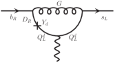
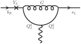
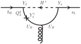
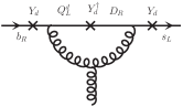
The case of $\Delta C_{7}^{(\prime)}$ is different. In Ref. Blanke:2012tv a determination of this coefficient in the RS model with and without custodial protection has been carried out directly in 5D, using the mixed position/momentum formalism. This approach includes the contribution of the whole tower of KK excitations. However, since the other coefficients used in this paper have been computed in the effective 4D model, we have repeated the calculation for $C_{7}(M_{KK})$ in 4D, as described in Appendix C, with a set of assumptions concerning the contributions of the KK excitations consistent with the calculation of $\Delta C_{9,10}^{(\prime)}$. In particular, we have kept only the dominant contribution of the first KK mode in the case of the intermediate gluon and Higgs fields exchanged in the diagrams in Fig. 18. For the intermediate fermions, consistently with the procedure described in the previous Section we have included only the zero modes. For the evolution at the scale $\mu_{b}$, we use the master formula Blanke:2012tv :

$$\Delta C_{7}^{(\prime)}(\mu_{b})=0.429\,\Delta C_{7}^{(\prime)}(M_{KK})+0.128\,\Delta C_{8}^{(\prime)}(M_{KK})\,\,$$ (44)

which shows that $\Delta C_{8}^{(\prime)}(M_{KK})$ are needed; they are also computed in Appendix C.

V Numerical analysis

The results for the observables considered in this paper within the RS_c model are obtained adding the new contributions to the Wilson coefficients computed scanning the parameter space of the model. In particular, we focus on the elements of the two Yukawa matrices $\lambda^{d,u}$, and on the bulk mass parameters for quarks and leptons.

The diagonal elements of $\lambda^{d,u}$ are fixed from the relations (38) (and the analogous ones for down-type quarks), so that, under the assumptions described in Sec. III, we scan over the two sets in Eq.(39). As customary for these scenarios, the requirement of perturbativity of the model up to the scale of the first three KK modes sets the range: $|\lambda^{d,u}_{ij}|\leq 3/k$. However, not all the values in this range are acceptable, since also the CKM matrix elements should be reproduced after the constraint $V_{CKM}={\cal U}_{L}^{\dagger}{\cal D}_{L}$ is imposed. The first step in the parameter selection consists in fixing the bulk mass terms $c_{i}$ for down- and up-type quarks. Several analyses have been devoted to this purpose in the literature. We adopt the strategy outlined in buras1 and the consequent choice of parameters Duling:2010lqa . It consists in imposing that quark mass parameters at the high scale ${\cal O}(M_{KK})$, obtained from the $\overline{MS}$ masses using NLO renormalization group evolution, and CKM elements are reproduced within $2\sigma$. An exception is represented by the bulk mass parameter of the left-handed doublet of the third generation of quarks. We slightly vary it in a range which also satisfies the constraints derived in neubertRS exploiting the experimental measurements of several quantities related to $Z$ decays to $b$ quarks, i.e. the coupling $Z{\bar{b}}b$, the $b$-quark left-right asymmetry parameter and the forward-backward asymmetry for $b$ quarks ALEPH:2005ab . The set used in our analysis is :

$$c_{L}^{u,d}=0.63\,\,,\hskip 8.5359ptc_{L}^{c,s}=0.57\,\,,\hskip 8.5359ptc_{L}^{b,t}\in[0.40,\,0.45]\,\,,\,\,\,$$

$$c_{R}^{u}=0.67\,\,,\hskip 8.5359ptc_{R}^{c}=0.53\,\,,\hskip 8.5359ptc_{R}^{t}=-0.35\,\,,\,\,\,\,\,$$ (45)

$$c_{R}^{d}=0.66\,\,,\hskip 8.5359ptc_{R}^{s}=0.60\,\,,\hskip 8.5359ptc_{R}^{b}=0.57\,\,\,\,.\,\,\,\,\,\,\,\,\,$$

For leptons, $c_{\ell}$ are set to $c_{\ell}=0.7$ in all cases, motivated by the observation that lepton flavour-conserving couplings are almost independent of the choice of their bulk mass parameter provided that $c_{\ell}>0.5$ buras2 . Other determinations can be found in Huber:2000ie ; burdman ; agashe ; Agashe:2004ay ; Fitzpatrick:2007sa ; neubertRS ; Archer:2011bk .

Fixed such values, we generate the six $\lambda$ parameters in (39) which also satisfy the CKM constraints. In particular, we impose $|V_{cb}|$ and $|V_{ub}|$ in the largest range found from their experimental determinations from inclusive and exclusive $B$ decays Amhis:2012bh , and impose that $|V_{us}|$ lies within $2\%$ of the central value quoted by PDG Beringer:1900zz :

$$|V_{cb}| \in [0.038,\,0.043],$$

$$|V_{ub}| \in [0.00294,\,0.00434],$$ (46)

$$|V_{us}| \in [0.22,\,0.23].$$

For the quark masses we use

$$m_{d}=4.9\,\,{\rm MeV},\hskip 2.84544ptm_{s}=90\,\,{\rm MeV},\hskip 2.84544ptm_{b}=4.8\,\,{\rm GeV}\,\,\,.$$ (47)

Figure 1: $\Delta C_{7}(m_{b})$ vs $\Delta C_{9}$ obtained implementing sequentially the constraints described in the text. The light green points correspond to the constraints from $|V_{us}|$ and $|V_{ub}|$, the red points to the constraint from $|V_{cb}|$ and $|V_{ub}|$, the blue points to the further constraints from ${\cal B}(B\to K^{*}\mu^{+}\mu^{-})_{exp}$ and ${\cal B}(B\to X_{s}\gamma)_{exp}$.

These constraints are the starting point of our analysis. The generated values of the parameters fulfilling all the constraints are used to compute the RS contributions to the Wilson coefficients. Two further conditions on the computed $B\to K^{*}\mu^{+}\mu^{-}$ and $B\to X_{s}\gamma$ branching fractions are imposed, requiring that they are less than $2\sigma$ from the experimental measurements

$$\hskip-5.69046pt{\cal B}(B\to K^{*}\mu^{+}\mu^{-})_{exp} = (1.02\pm^{0.14}_{0.13}\pm 0.05)\times 10^{-6}\,,\,\,\,\,\,$$ (48)

$$\hskip-5.69046pt{\cal B}(B\to X_{s}\gamma)_{exp} = (3.43\pm 0.21\pm 0.07)\times 10^{-4};\,\,\,\,\,\,\,\,$$ (49)

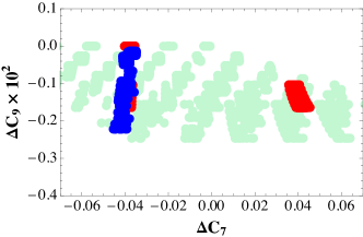
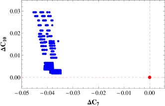
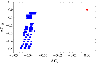
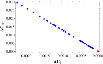
the result in (48) is the average performed by BaBar Collaboration of the branching fractions of the four modes $B^{+,0}\to K^{*+,0}\mu^{+}\mu^{-}(e^{+}e^{-})$ Lees:2012tva , while the result in (49) is the HFAG Collaboration average Amhis:2012bh . An example of the sequence of the effects of the constraints is shown in Fig.1. After imposing the constraints on $V_{ub}$ and $V_{us}$, a set of values of $\Delta C_{7}(m_{b})$ and $\Delta C_{9}$ is computed, and $\Delta C_{7}(m_{b})$ spans a quite broad range of positive and negative values, the green region in the figure. Implementing the constraint on $V_{cb}$ reduces the possibilities to two isolated regions, the red spots in the figure, and the region of negative values, the blue one, survives after the constraints (48) and (49) are imposed. We have checked that the selected points reproduce also the other CKM elements within their uncertainty, except for $|V_{td}|$ which lies in the $3\sigma$ range around its central value Beringer:1900zz . Moreover, as discussed in buras1 , the set of parameters selected imposing the quark masses and CKM constraints allows to satisfy also the constraint from ${\bar{B}}_{s}-B_{s}$ mixing. On the basis of this we have not repeated such an analysis, considering that we also impose that the data in (48-49) are reproduced, which usually represent more severe conditions.

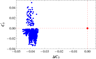
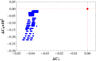
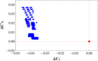
We depict in Fig.2 the obtained values and correlations for $\Delta C_{i}^{(\prime)}$. The largest deviations from the SM are $|\Delta C_{7}|_{max}\simeq 0.046\,$, $|\Delta C_{7}^{\prime}|_{max}\simeq 0.05\,$, $|\Delta C_{9}|_{max}\simeq 0.0023\,$, $|\Delta C_{9}^{\prime}|_{max}\simeq 0.038\,$, $|\Delta C_{10}|_{max}\simeq 0.030\,$, $|\Delta C_{10}^{\prime}|_{max}\simeq 0.50\,$. As shown in the panel $(f)$ of the figure, $\Delta C_{9}$ and $\Delta C_{10}$ are linearly correlated, and the same happens for each pair $\Delta C_{i}^{(\prime)}$, $i=9,10$. Indeed, in the large set of parameters the most relevant input for these coefficients is $\lambda_{23}^{d}$, and the relations approximately hold (for $c_{L}^{b,t}$ fixed to the central value):

$$\Delta C_{9} \simeq -7.18\,10^{-4}\,\lambda_{23}^{d}\,k$$

$$\Delta C_{9}^{\prime} \simeq 1.22\,10^{-2}\,\lambda_{23}^{d}\,k$$

$$\Delta C_{10} \simeq 9.55\,10^{-3}\,\lambda_{23}^{d}\,k$$ (50)

$$\Delta C_{10}^{\prime} \simeq -1.62\,10^{-1}\,\lambda_{23}^{d}\,k\,\,.$$

(a)	(b)
(c)	(d)
(e)	(f)

Figure 2: Correlations between the RS_c contribution to the Wilson coefficients $C_{7,9,10}^{(\prime)}$. The coefficients $\Delta C_{7}^{(\prime)}$ are evaluated at the scale $\mu_{b}=m_{b}$. No correction corresponds to the red dot.

There have been attempts to understand what would be the required size of deviations from SM values for the Wilson coefficients that could explain the observed anomalies in $B\to K^{*}\mu^{+}\mu^{-}$ distributions (on which we shall elaborate below) and, consequently, which NP scenario might provide such deviations Descotes-Genon:2013wba ; Altmannshofer:2013foa ; Beaujean:2013soa . Although there is not a unique answer to this question, a possible conclusion is that NP should provide a large negative value of $\Delta C_{9}$. For example, in Altmannshofer:2013foa various possibilities are considered in which NP affects just one Wilson coefficient, a pair of them, or all of them simultaneously. In the last case, to which the RS scenario belongs, it is found that the required deviation of $C_{9}$ from its SM value should be $\Delta C_{9}\simeq-0.9$ for a real coefficient, or even $|\Delta C_{9}|\simeq 2.25$ for a complex one. The result of our analysis shows that such a huge deviation is not reached in RS_c, as in the NP models considered so far for this purpose. The largest deviations (still not sizable enough) are found in models introducing a new neutral gauge boson $Z^{\prime}$ with suitable FCNC couplings to quarks Buras:2013qja ; Buras:2013dea ; Gauld:2013qba .

VI $B^{0}\to K^{*0}\ell^{+}\ell^{-}$ observables

It is now possible to compute the set of $B\to K^{*}\mu^{+}\mu^{-}$ observables measured by LHCb, and compare the outcome with data. The results are collected in Figs.3-8. The results obtained in SM include the uncertainty in the hadronic form factors; for such nonperturbative quantities we use the light-cone QCD sum rule determination in Ball:2004rg (previous determinations, such as the one in Colangelo:1995jv , have larger uncertainties). The hadronic errors have an impact mainly on the $B^{0}\to K^{*0}\mu^{+}\mu^{-}$ differential decay rate and on the $K^{*}$ longitudinal polarization distribution, while to position of the zero in $A_{FB}(q^{2})$ and of the maximum of $F_{L}$ are less affected, as expected.

Figure 3: Differential $B^{0}\to K^{*0}\mu^{+}\mu^{-}$ decay rate. The light (green) band corresponds to the SM result, including the uncertainty of the form factors. The red and blue vertical bars correspond to the RS_c result, without or with the uncertainty in form factors. The black dots, with their error bars, are the LHCb measurements in Aaij:2013iag .

Figure 4: Lepton FB asymmetry in $B^{0}\to K^{*0}\mu^{+}\mu^{-}$. The symbols have the same meaning as in Fig. 3.

Figure 5: $K^{*}$ longitudinal polarization fraction in $B^{0}\to K^{*0}\mu^{+}\mu^{-}$. The symbols have the same meaning as in Fig. 3.

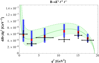
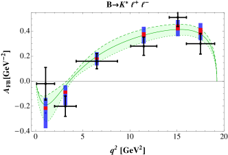
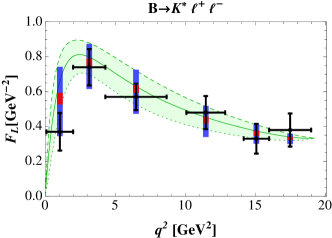
In the analysis of the modifications in RS_c, for the various observables, we separately consider the changes due to the new Wilson coefficients, and the changes which also include the hadronic form factor uncertainties. The results show that the deviations induced in RS_c are small, since the corrections $\Delta C_{9,10}$ are tiny fractions of $C_{9,10}^{SM}$ and that also the coefficients of operators absent in SM, $\Delta C^{\prime}_{9,10}$ are small. A little effect is found at small $q^{2}$, where the changes due to $\Delta C_{7}^{(\prime)}$ are slightly larger. The comparison of data with predictions confirmes the agreement, excluding the measurement of $A_{FB}(q^{2})$ in the first bin of $q^{2}$ where the predictions are larger than the experimental result. In the high $q^{2}$ range the hadronic uncertainty for the lepton FB asymmetry is about $20\%$.

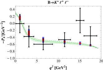
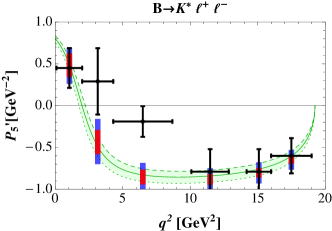
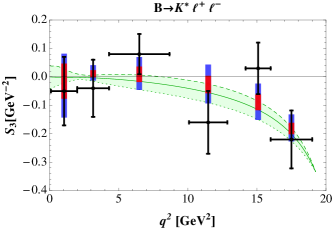
The results for the observables $P^{\prime}_{4}$, $P^{\prime}_{5}$ and $S_{3}$ are shown in Figs. 6, 7 and 8. In $P^{\prime}_{5}$ the hadronic uncertainty is at the level of $10\%$ in all the $q^{2}$ range. The modification of the prediction obtained in RS_c is similar or larger at low $q^{2}$, up to $q^{2}\simeq 7$ GeV², therefore this is a favourable kinematical range where to investigate this observable. The discrepancy with the measurement in the third $q^{2}$ bin still persists, while there is agreement in the other bins.

The hadronic uncertainties turn out to be smaller in $P^{\prime}_{4}$, and the changes in the predictions in RS_c seem promising to be observed at low $q^{2}$. A deviation observed in the fifth $q^{2}$ bin of the series of measurements is at the level of less than $2\sigma$.

At odds with $P^{\prime}_{5}$, in the observable $S_{3}$ the RS_c result is systematically above the SM for the largest part of the parameter space, in particular in the large $q^{2}$ range, as shown in Fig. 8. The size of such effect is comparable with the hadronic uncertainty; therefore, one can envisage the possibility of using this observable for a better characterization of the deviations obtained in this new physics scenario. The experimental results follow the predictions, but the errors are too large to draw conclusions. All the observations can be quantified as done in Table 1, which confirms that the largest deviation in the measured observables occurs in $P_{5}^{\prime}$.

Figure 6: Observable $P^{\prime}_{4}$ in $B^{0}\to K^{*0}\mu^{+}\mu^{-}$. The light (green) band corresponds to the SM result, including the uncertainty of the form factors. The red and blue vertical bars correspond to the RS_c result, without or with the uncertainty in form factors. The black dots, with their error bars, are the LHCb measurements in Ref. Aaij:2013qta . The sign is fixed to make the definition (16) and the one in Ref. Aaij:2013qta compatible.

Figure 7: Observable $P^{\prime}_{5}$ in $B^{0}\to K^{*0}\mu^{+}\mu^{-}$. The meaning of the symbols is the same as in Fig. 6.

Figure 8: Observable $S_{3}$ in $B^{0}\to K^{*0}\mu^{+}\mu^{-}$. The symbols have the same meaning as in Fig. 3.

	$d{\cal B}/dq^{2}$	$F_{L}$	${\cal A}_{FB}$	$P_{4}^{\prime}$	$P_{5}^{\prime}$	$S_{3}$
$\chi^{2}$	$0.49$	$0.19$	$0.79$	$0.91$	$2.09$	$0.53$

Table 1: $\chi^{2}$ values for the various observables, defined as $\displaystyle\chi^{2}=\frac{1}{N}\sum_{i}^{N}\frac{\left({\cal O}^{\text{exp}}_{i}-{\cal O}^{\text{th}}_{i}\right)^{2}}{\delta_{i}^{2}+\sigma_{i}^{2}}$. $i$ runs over the $N$ experimental bins, ${{\cal O}^{\text{exp}}_{i}}$ and ${\cal O}^{\text{th}}_{i}$ are the LHCb measurements and the theoretical results in the RS_c model, with errors $\delta_{i}$ and $\sigma_{i}$, respectively.

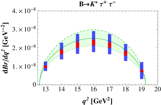
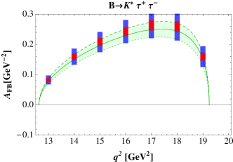
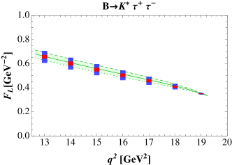
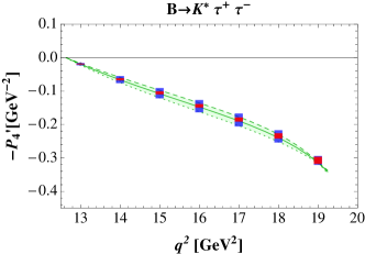
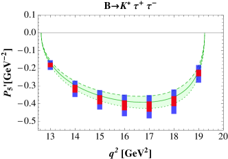
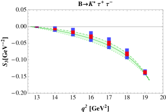
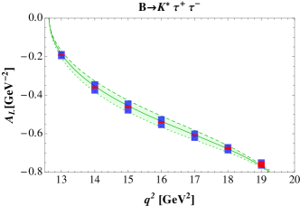
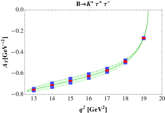
The results for the case of $\tau^{+}\tau^{-}$ final state are shown in Figs. 9-14. The kinematically accessible $q^{2}$ range starts at $q^{2}\simeq 12.628$ GeV², so that the small effects in the muon mode at low $q^{2}$ do not appear in this case. In the decay rate distribution and in the lepton FB asymmetry the results in RS_c systematically deviate from SM in the full parameter space, but the effect is smaller than the hadronic uncertainty. Such a systematic deviation also appears in $P^{\prime}_{5}$ and $S_{3}$, Fig.13 and 14, while the longitudinal and transverse $\tau$ polarization asymmetries essentially coincide with the SM ones, Fig.15, and seem not suitable for characterizing the considered new physics model.

Figure 9: Differential $B\to K^{*}\tau^{+}\tau^{-}$ decay rate. The light (green) band corresponds to the SM result, including the uncertainty in the form factors. The red and blue vertical bars correspond to the RS_c result, without or with the uncertainty in form factors.

Figure 10: Lepton FB asymmetry in $B\to K^{*}\tau^{+}\tau^{-}$. The symbols have the same meaning as in Fig. 9.

Figure 11: $K^{*}$ longitudinal polarization fraction in $B\to K^{*}\tau^{+}\tau^{-}$. The symbols have the same meaning as in Fig. 9.

Figure 12: Observable $P^{\prime}_{4}$ in $B\to K^{*}\tau^{+}\tau^{-}$. The symbols have the same meaning as in Fig. 9. The sign is fixed to make compatible the definition (16) and the one adopted in Ref. Aaij:2013qta , as in the case of $\mu^{+}\mu^{-}$.

Figure 13: Observable $P^{\prime}_{5}$ in $B\to K^{*}\tau^{+}\tau^{-}$. The symbols have the same meaning as in Fig. 9.

Figure 14: Observable $S_{3}$ in $B\to K^{*}\tau^{+}\tau^{-}$. The symbols have the same meaning as in Fig. 9.

Figure 15: Longitudinal and transverse $\tau$ polarization asymmetries. The symbols have the same meaning as in Fig. 9.

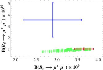
A final remark concerns the rare $B_{s,d}\to\mu^{+}\mu^{-}$ modes. As stated in the Introduction, an important breakthrough is the measurement in Eq. (1). Since the theoretical predictions for the branching fractions of these modes depend on a subset of the Wilson coefficients that have been considered, we can derive predictions using the same set of parameters, see Fig. 16. The SM result depends only on the coefficient $C_{10}$, and in RS one has to replace $C_{10}\to C_{10}-C_{10}^{\prime}$. In Fig. 16 we show the correlation between the two modes, comparing the RS prediction to SM and to the experimental data. There is a region of the parameter space in which the SM result for both branching ratios is reproduced. However, the allowed range in RS_c is larger than in SM: ${\cal B}(B_{s}\to\mu^{+}\mu^{-})|_{RS}\in[2.64,\,3.83]\,\times 10^{-9}$ and ${\cal B}(B_{d}\to\mu^{+}\mu^{-})|_{RS}\in[0.70,\,1.16]\,\times 10^{-10}$, in the right direction in the case of $B_{s}$ when comparing with data, but still lower than the datum for $B_{d}$. A similar result was already found in buras2 , although with a smaller deviation with respect to SM, in particular in the $B_{s}$ case.

Figure 16: Correlation between the branching ratios of $B_{s}\to\mu^{+}\mu^{-}$ and $B_{d}\to\mu^{+}\mu^{-}$. The blue bars represent the experimental data (1), the red ones the SM predictions (2). The green region is the prediction in RS_c derived in this paper.

VII Conclusions

We have studied several observables of the rare decays $B\to K^{*}\ell^{+}\ell^{-}$ within the RS_c model, in the case where measurements are available and in the case of massive leptons. We have carried out a new calculation of the contributions to the Wilson coefficients $C^{(\prime)}_{7,8}$ and a new scan of the model parameters, imposing the experimental constraints of CKM and quark mass values. The obtained deviations with respect SM are small, and at present they are generally hidden by the uncertainties on the hadronic form factors for several observables. However, in few cases the deviations from SM are systematic in the full $q^{2}$ range, and are similar to the presently accepted hadronic uncertainties: this renders such observables of great interest in view of searching signals of this possible extension of the Standard Model.

Appendix A Gauge boson and fermion profiles

The gauge boson and fermion profiles, entering in the calculations carried out in this paper, are obtained solving the equations of motion for the corresponding fields Davoudiasl:1999tf ; gherghetta :

• profile of the first KK excitation of a gauge boson having a zero mode

  $$g(y)=\frac{e^{ky}}{N_{1}}\left[J_{1}\left(\frac{m_{1}}{k}e^{ky}\right)+b_{1}(m_{1})Y_{1}\left(\frac{m_{1}}{k}e^{ky}\right)\right]\,\,\,,$$ (51)

  with $J_{1}$ and $Y_{1}$ Bessel functions,

  $$b_{1}(m_{1}) = -\frac{J_{1}\left(\frac{m_{1}}{k}\right)+\frac{m_{1}}{k}J_{1}^{\prime}\left(\frac{m_{1}}{k}\right)}{Y_{1}\left(\frac{m_{1}}{k}\right)+\frac{m_{1}}{k}Y_{1}^{\prime}\left(\frac{m_{1}}{k}\right)}\,\,\,,$$ (52)

  $$N_{1} = \frac{e^{kL/2}}{\sqrt{\pi Lm_{1}}}\,\,\,.$$ (53)

  We use $m_{1}\simeq 2.45\,f$.

• profile of the first KK level of a gauge boson without zero mode

  $${\tilde{g}}(y)=\frac{e^{ky}}{N_{1}}\left[J_{1}\left(\frac{\tilde{m}_{1}}{k}e^{ky}\right)+\tilde{b}_{1}(\tilde{m}_{1})Y_{1}\left(\frac{\tilde{m}_{1}}{k}e^{ky}\right)\right]$$ (54)

  where now

  $$\tilde{b}_{1}(\tilde{m}_{1})=-\frac{J_{1}\left(\frac{\tilde{m}_{1}}{k}\right)}{Y_{1}\left(\frac{\tilde{m}_{1}}{k}\right)}\,\,\,.$$ (55)

  We use $\tilde{m}_{1}\simeq 2.40\,f$.

• profile of the fermion zero mode

  $$f^{(0)}(y,c)=\sqrt{\frac{(1-2c)kL}{e^{(1-2c)kL}-1}}e^{-cky}\,\,.$$ (56)

Appendix B Feynman rules for neutral current interactions

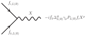
We need to consider the neutral current interactions mediated by the gauge bosons $Z,\,Z_{H},\,Z^{\prime}$ and $A^{(1)}$. As mentioned, such interactions can be either flavour conserving or flavour violating. We collect in four triplets the up-type quarks, the down-type quarks, the neutrinos and the charged leptons: $f=\left(\begin{array}[]{c}f_{1}\\ f_{2}\\ f_{3}\end{array}\right),$ with $f=u_{i},\,d_{i},\,\nu_{\ell_{i}},\ell_{i}^{-}$, and $i=1,2,3$ a generation index. We define the effective coupling of a generic gauge boson $X$ to a pair of fermions $f_{i}\,f_{k}$:

$${\cal L}_{int}^{X}=-iX^{\mu}\left(\Delta_{L}^{f_{i}f_{k}}{\bar{f}}_{k,L}\gamma_{\mu}P_{L}f_{i,L}+\Delta_{R}^{f_{i}f_{k}}{\bar{f}}_{k,L}\gamma_{\mu}P_{R}f_{i,L}\right)\,\,,$$ (57)

where $\displaystyle P_{L,R}=\frac{1\mp\gamma_{5}}{2}$. Fig. 17 shows this vertex. In the expression of the couplings $\Delta_{L,R}^{f_{i}f_{k}}$, two more overlap integrals are needed:

$$I_{1}^{+} = \frac{1}{L}\int_{0}^{L}dy\,e^{-2ky}[h(y)]^{2}\,g(y)\,\,,$$

$$I_{1}^{-} = \frac{1}{L}\int_{0}^{L}dy\,e^{-2ky}[h(y)]^{2}\,{\tilde{g}}(y)\,\,,$$ (58)

together with the quantity

$$D^{f_{i}f_{k}}=\tilde{\cal R}_{f_{i}f_{k}}I_{1}^{-}-{\cal R}_{f_{i}f_{k}}I_{1}^{+}\,\,.$$ (59)

$D^{f}$ is the diagonal matrix with elements $D^{f_{i}f_{i}}$. We consider separately the case of the four neutral gauge bosons listed above. In the following, ${\cal M}$ indicates one of the matrices ${\cal U}_{L}$, ${\cal U}_{R}$, ${\cal D}_{L}$, ${\cal D}_{R}$, for up or down-type left- and right-handed quarks. The obtained rules also hold in the case of leptons with ${\cal M}$ being the unit matrix. In the case of the couplings of $Z$, $Z^{\prime}$ and $Z_{H}$ the Feynman rules are obtained expanding in the small parameter $\displaystyle\epsilon=\frac{g^{2}v^{2}}{4LM^{2}}$, with $g$ the $5D$ $SU(2)_{L}$ gauge constant and $M^{2}=(m_{1}^{2}+{\tilde{m}}_{1}^{2})/2$. Since, neglecting corrections of ${\cal O}(v^{2}/M^{2})$ the mixing angle $\psi$ in (30-31) coincides with the Weinberg angle $\theta_{W}$, in the following Feynman rules we put $s_{\psi}=s_{W}=\sin\theta_{W}$ and $c_{\psi}=c_{W}=\cos\theta_{W}$.

Figure 17: Couplings of neutral gauge bosons $X=Z,\,Z_{H},\,Z^{\prime},\,A^{(1)}$ to fermions $f$ with flavour indices $i,k$. In addition to flavour conserving couplings, $i=k$, flavour violating couplings $i\neq k$ are possible.

• Couplings of the photon 1-mode $A^{(1)}$

  The couplings are given by

  $$\Delta_{L}^{f_{i}f_{k}}(A^{(1)})=\Delta_{R}^{f_{i}f_{k}}(A^{(1)})=Q_{f}\,e\left({\cal M}^{\dagger}{\cal R}_{f}{\cal M}\right)_{ki}$$ (60)

  where $Q_{f}$ is the electric charge of the fermion $f$ (in units of the positron charge $e$).
  

• $Z$ couplings

  In terms of the SM couplings of the $Z$ boson:

  $$[g_{Z}^{SM}(f)]=-\frac{e}{s_{W}c_{W}}\left(T_{3}-s_{W}^{2}Q_{f}\right)\,\,\,,$$ (61)

  with $T_{3}$ the third component of the weak $SU(2)_{L}$ isospin, we find:

  $$\Delta^{f_{i}f_{k}}(Z)\hskip 142.26378pt$$

  $$=[g_{Z}^{SM}(f)]\left\{\delta_{ki}+\frac{\epsilon}{c^{2}_{W}}\left({\cal M}^{\dagger}D^{f}{\cal M}\right)_{ki}\right\}$$ (62)

  for $f=u_{R},\,c_{R},\,t_{R}$, for $f=d_{L},\,s_{L},\,b_{L}$, and for $f=\ell^{-}_{L}$, and

  $$\Delta^{f_{i}f_{k}}(Z)\hskip 142.26378pt$$

  $$=[g_{Z}^{SM}(f)]\left\{\delta_{ki}+\frac{\epsilon}{c^{2}_{W}}\left({\cal M}^{\dagger}D^{f}{\cal M}\right)_{ki}\right\}$$

  $$+\frac{\epsilon e}{s_{W}c_{W}}I_{1}^{-}\left({\cal M}^{\dagger}\tilde{\cal R}_{f}{\cal M}\right)_{ki}\hskip 62.59596pt$$ (63)

  for $f=u_{L},c_{L},t_{L}$, for $f=d_{R},s_{R},b_{R}$, and for $f=\ell^{-}_{R},\nu_{e,\,\mu,\,\tau}$.

• $Z_{H}$ couplings

  At the order ${\cal O}(\epsilon^{0})$ for the heavier bosons $Z_{H}$ and $Z^{\prime}$ we find:

  $$\Delta^{f_{i}f_{k}}(Z_{H})=c_{\xi}(\Delta_{f}^{c})_{ki}(Z_{H})+s_{\xi}(\Delta_{f}^{s})_{ki}(Z_{H})\,,$$ (64)

  where $c_{\xi}=\cos(\xi)$ and $s_{\xi}=\sin(\xi)$, and

  $$(\Delta_{f}^{c})_{ij}(Z_{H}) = g_{Z}^{SM}(f)\left({\cal M}^{\dagger}{\cal R}_{f}{\cal M}\right)_{ij}\,\,\,,$$

  $$(\Delta_{f}^{s})_{ij}(Z_{H}) = \frac{\left({\cal M}^{\dagger}\tilde{\cal R}_{f}{\cal M}\right)_{ij}}{\sqrt{1-2s_{W}^{2}}}\left[g_{Z}^{SM}(f)+gc_{W}\right],$$ (65)

  for $f=u_{L},c_{L},t_{L}$, and for $f=d_{R},s_{R},b_{R}$, and

  $$(\Delta_{f}^{c})_{ij}(Z_{H}) = g_{Z}^{SM}(f)\left({\cal M}^{\dagger}{\cal R}_{f}{\cal M}\right)_{ij}\,\,\,,$$

  $$(\Delta_{f}^{s})_{ij}(Z_{H}) = \frac{\left({\cal M}^{\dagger}\tilde{\cal R}_{f}{\cal M}\right)_{ij}}{\sqrt{1-2s_{W}^{2}}}g_{Z}^{SM}(f)\,\,\,,$$ (66)

  for $f=u_{R},c_{R},t_{R}$, and for $f=d_{L},s_{L},b_{L}$. For leptons we have:

  $$\Delta^{\ell\ell}(Z_{H})\hskip 156.49014pt$$

  $$=g_{Z}^{SM}(\ell)\left[c_{\xi}\Delta^{c,\ell\ell}(Z_{H})+s_{\xi}\Delta^{s,\ell\ell}(Z_{H})\right]\,,$$ (67)

  where

  $$\Delta^{c,\ell\ell}(Z_{H}) = {\cal R}_{\ell\ell}\hskip 42.67912pt(\ell=\nu,\ell^{-}_{L},\ell^{-}_{R})$$

  $$\Delta^{s,\nu\nu}(Z_{H}) = -\tilde{\cal R}_{\nu\nu}\sqrt{1-2s_{W}^{2}}$$

  $$\Delta^{s,\ell^{-}_{L}\ell^{+}_{L}}(Z_{H}) = \frac{\tilde{\cal R}_{\ell^{-}_{L}\ell^{+}_{L}}}{\sqrt{1-2s_{W}^{2}}}$$ (68)

  $$\Delta^{s,\ell^{-}_{R}\ell^{+}_{R}}(Z_{H}) = -\tilde{\cal R}_{\ell^{-}_{R}\ell^{+}_{R}}\frac{\sqrt{1-2s_{W}^{2}}}{s^{2}_{W}}\,\,\,.$$

• $Z^{\prime}$ couplings

  Defining the couplings with the same structure as in Eq.(64), we find:

  $$(\Delta_{f}^{c})_{ij}(Z^{\prime}) = (\Delta_{f}^{s})_{ij}(Z_{H})$$

  $$(\Delta_{f}^{s})_{ij}(Z^{\prime}) = -(\Delta_{f}^{c})_{ij}(Z_{H})\,\,\,.$$ (69)

  For leptons we have

  $$\Delta^{c,\ell\ell}(Z^{\prime}) = \Delta^{s,\ell\ell}(Z_{H})$$

  $$\Delta^{s,\ell\ell} = -\Delta^{c,\ell\ell}(Z_{H})\,\,\,.$$ (70)

Appendix C Calculation of $\Delta C_{7,8}^{(\prime)}$ at the high scale $M_{KK}$

$(\Delta C_{7}^{(\prime)})_{1}$	$(\Delta C_{7}^{(\prime)})_{2}$	$(\Delta C_{7}^{(\prime)})_{3}$
$(\Delta C_{8}^{(\prime)})_{1}$	$(\Delta C_{8}^{(\prime)})_{2}$	$(\Delta C_{8}^{(\prime)})_{3}$

Figure 18: New penguin diagrams contributing to the Wilson coefficients $C_{7,8}^{(\prime)}$ in the RS_c model. Diagrams with specular mass insertions must also be considered.

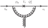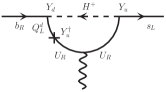
To compute $\Delta C_{7,8}^{(\prime)}$ at the scale $M_{KK}$ one has to consider penguin diagrams with new particles in addition to the SM ones. In the approximation adopted in this paper of neglecting higher KK modes for fermions, the dominant diagrams (shown in Fig. 18) are of the following type Csaki:2010aj ; Blanke:2012tv :

• Penguin diagrams mediated by a charged Higgs in which a photon (for $C_{7}^{(\prime)}$) or a gluon (for $C_{8}^{(\prime)}$) is emitted from an internal up-type quark, with a mass insertion on the internal fermion line. Diagrams contributing to the primed coefficients differ from those for the unprimed for the chirality of the external quarks.

• Penguin diagrams mediated by a gluon with an internal down-type quark. For $C_{7}^{(\prime)}$ we have the contributions $(\Delta C_{7}^{(\prime)})_{2}$ and $(\Delta C_{7}^{(\prime)})_{3}$ as in Fig. 18, for $C_{8}^{(\prime)}$ the contributions $(\Delta C_{8}^{(\prime)})_{2}$ and $(\Delta C_{8}^{(\prime)})_{3}$ involve the three-gluon vertex.

We list below the results.

$$(\Delta C_{7})_{1} = i\,Q_{u}\,r\,\sum_{F=u,c,t}\left[A+2m_{F}^{2}(A^{\prime}+B^{\prime})\right]\left[{\cal D}_{L}^{\dagger}Y^{u}(Y^{u})^{\dagger}Y^{d}{\cal D}_{R}\right]_{23}$$

$$(\Delta C_{7})_{2} = -i\,Q_{d}\,r\frac{8}{3}(g_{s}^{4D})^{2}\,\sum_{F=d,s,b}\left[I_{0}+A+B+4m_{F}^{2}(I_{0}^{\prime}+A^{\prime}+B^{\prime})\right]\left[{\cal D}_{L}^{\dagger}{\cal R}_{L}Y^{d}{\cal R}_{R}{\cal D}_{R}\right]_{23}$$ (71)

$$(\Delta C_{7})_{3} = i\,Q_{d}\,r\frac{8}{3}(g_{s}^{4D})^{2}\,\sum_{F=d,s,b}\frac{m_{F}}{m_{b}}\,\left[I_{0}+A+B\right]\left\{\left[{\cal D}_{L}^{\dagger}{\cal R}_{L}{\cal R}_{L}Y^{d}{\cal D}_{R}\right]_{23}+\frac{m_{b}}{m_{s}}\left[{\cal D}_{L}^{\dagger}Y^{d}{\cal R}_{R}{\cal R}_{R}{\cal D}_{R}\right]_{23}\right\}$$

$$(\Delta C_{7}^{\prime})_{1} = i\,Q_{u}\,r\,\sum_{F=u,c,t}\left[A+2m_{F}^{2}(A^{\prime}+B^{\prime})\right]\left[{\cal D}_{R}^{\dagger}(Y^{d})^{\dagger}Y^{u}(Y^{u})^{\dagger}{\cal D}_{L}\right]_{23}$$

$$(\Delta C_{7}^{\prime})_{2} = -i\,Q_{d}\,r\frac{8}{3}(g_{s}^{4D})^{2}\,\sum_{F=d,s,b}\left[I_{0}+A+B+4m_{F}^{2}(I_{0}^{\prime}+A^{\prime}+B^{\prime})\right]\left[{\cal D}_{R}^{\dagger}{\cal R}_{R}(Y^{d})^{\dagger}{\cal R}_{L}{\cal D}_{L}\right]_{23}$$ (72)

$$(\Delta C_{7}^{\prime})_{3} = i\,Q_{d}\,r\frac{8}{3}(g_{s}^{4D})^{2}\,\sum_{F=d,s,b}\frac{m_{F}}{m_{b}}\,\left[I_{0}+A+B\right]\left\{\left[{\cal D}_{R}^{\dagger}{\cal R}_{R}{\cal R}_{R}(Y^{d})^{\dagger}{\cal D}_{L}\right]_{23}+\frac{m_{b}}{m_{s}}\left[{\cal D}_{R}^{\dagger}(Y^{d})^{\dagger}{\cal R}_{L}{\cal R}_{L}{\cal D}_{L}\right]_{23}\right\}$$

$$(\Delta C_{8})_{1} = i\,r\,\sum_{F=u,c,t}\left[{A}+2m_{F}^{2}({A}^{\prime}+{B}^{\prime})\right]\left[{\cal D}_{L}^{\dagger}Y^{u}(Y^{u})^{\dagger}Y^{d}{\cal D}_{R}\right]_{23}$$

$$(\Delta C_{8})_{2} = -i\,r\frac{9}{8}(g_{s}^{4D})^{2}\,\frac{v^{2}}{m_{b}\,m_{s}}\,{\cal T}_{3}\,\sum_{F=d,s,b}\left[{\bar{A}}+{\bar{B}}+2m_{F}^{2}({\bar{A}}^{\prime}+{\bar{B}}^{\prime})\right]\left[{\cal D}_{L}^{\dagger}Y^{d}{\cal R}_{R}(Y^{d})^{\dagger}{\cal R}_{L}Y^{d}{\cal D}_{R}\right]_{23}$$ (73)

$$(\Delta C_{8})_{3} = -i\,\,r\,\frac{9}{4}(g_{s}^{4D})^{2}\,{\cal T}_{3}\,\sum_{F=d,s,b}\left[{\bar{A}}+{\bar{B}}+2m_{F}^{2}({\bar{A}}^{\prime}+{\bar{B}}^{\prime})\right]\left[{\cal D}_{L}^{\dagger}{\cal R}_{L}Y^{d}{\cal R}_{R}{\cal D}_{R}\right]_{23}$$

$$(\Delta C_{8}^{\prime})_{1} = i\,r\,\sum_{F=u,c,t}\left[{A}+2m_{F}^{2}({A}^{\prime}+{B}^{\prime})\right]\left[{\cal D}_{R}^{\dagger}(Y^{d})^{\dagger}Y^{u}(Y^{u})^{\dagger}{\cal D}_{L}\right]_{23}$$

$$(\Delta C_{8}^{\prime})_{2} = -i\,r\frac{9}{8}(g_{s}^{4D})^{2}\,\frac{v^{2}}{m_{b}\,m_{s}}\,{\cal T}_{3}\,\sum_{F=d,s,b}\left[{\bar{A}}+{\bar{B}}+2m_{F}^{2}({\bar{A}}^{\prime}+{\bar{B}}^{\prime})\right]\left[{\cal D}_{R}^{\dagger}(Y^{d})^{\dagger}{\cal R}_{L}Y^{d}{\cal R}_{R}(Y^{d})^{\dagger}{\cal D}_{L}\right]_{23}$$ (74)

$$(\Delta C_{8}^{\prime})_{3} = -i\,\,r\,\frac{9}{4}(g_{s}^{4D})^{2}\,{\cal T}_{3}\,\sum_{F=d,s,b}\left[{\bar{A}}+{\bar{B}}+2m_{F}^{2}({\bar{A}}^{\prime}+{\bar{B}}^{\prime})\right]\left[{\cal D}_{R}^{\dagger}{\cal R}_{R}(Y^{d})^{\dagger}{\cal R}_{L}{\cal D}_{L}\right]_{23}\,\,\,.$$

We have defined $\displaystyle r=\displaystyle{\frac{v}{\frac{G_{F}}{4\pi^{2}}\,V_{tb}\,V_{ts}^{*}\,m_{b}}}$ and ${\cal T}_{3}$ is the overlap of the profiles of two KK 1-mode and one KK 0-mode gluons: $\displaystyle{\cal T}_{3}=\frac{1}{L}\int_{0}^{L}dy[g(y)]^{2}$. $Q_{u}=\frac{2}{3}$ and $Q_{d}=-\frac{1}{3}$ are the up- and down-type quark electric charges in units of the positron charge $e$. The quantities $I_{0}^{(\prime)}$, $A^{(\prime)}$ and $B^{(\prime)}$ correspond to the loop integrals, and they are listed below.

$$I_{0}(t) = \frac{i}{(4\pi)^{2}}\,\frac{1}{M^{2}_{KK}}\left(-\frac{1}{t-1}+\frac{\ln(t)}{(t-1)^{2}}\right)$$

$$I_{0}^{\prime}(t) = \frac{i}{(4\pi)^{2}}\,\frac{1}{M^{4}_{KK}}\left(\frac{1+t}{2t(t-1)^{2}}-\frac{\ln(t)}{(t-1)^{3}}\right)$$

$$A(t) = B(t)=\frac{i}{(4\pi)^{2}}\,\frac{1}{4M^{2}_{KK}}\left(\frac{t-3}{(t-1)^{2}}+\frac{2\ln(t)}{(t-1)^{3}}\right)$$

$$A^{\prime}(t) = 2B^{\prime}(t)=\frac{i}{(4\pi)^{2}}\,\frac{1}{M^{4}_{KK}}\left(-\frac{t^{2}-5t-2}{6t(t-1)^{3}}-\frac{\ln(t)}{(t-1)^{4}}\right)$$ (75)

$${\bar{A}}(t) = {\bar{B}}(t)=\frac{i}{(4\pi)^{2}}\,\frac{1}{4M^{2}_{KK}}\left(-\frac{3t-1}{(t-1)^{2}}+\frac{2t^{2}\ln(t)}{(t-1)^{3}}\right)$$

$${\bar{A}}^{\prime}(t) = {\bar{B}}^{\prime}(t)=\frac{i}{(4\pi)^{2}}\,\frac{1}{4M^{4}_{KK}}\left(\frac{5t+1}{(t-1)^{3}}-\frac{2t(2+t)\ln(t)}{(t-1)^{4}}\right)\,\,\,,$$

with $t=m_{F}^{2}/M_{KK}^{2}$.

References

- (1) R. Aaij et al. [LHCb Collaboration], Phys. Rev. Lett. 111, 101805 (2013) [arXiv:1307.5024 [hep-ex]].
- (2) S. Chatrchyan et al. [CMS Collaboration], Phys. Rev. Lett. 111, 101804 (2013) [arXiv:1307.5025 [hep-ex]].
- (3) I. Dunietz, R. Fleischer and U. Nierste, Phys. Rev. D 63, 114015 (2001) [hep-ph/0012219].
- (4) C. Bobeth, M. Gorbahn, T. Hermann, M. Misiak, E. Stamou and M. Steinhauser, Phys. Rev. Lett. 112, 101801 (2014) [arXiv:1311.0903 [hep-ph]].
- (5) R. Aaij et al. [LHCb Collaboration], Phys. Rev. Lett. 108, 181806 (2012) [arXiv:1112.3515 [hep-ex]].
- (6) R. Aaij et al. [LHCb Collaboration], JHEP 1308, 131 (2013) [arXiv:1304.6325 [hep-ex]]].
- (7) R. Aaij et al. [LHCb Collaboration], Phys. Rev. Lett. 111, 191801 (2013) [arXiv:1308.1707 [hep-ex]].
- (8) A. Usanova [ATLAS Collaboration], PoS Beauty 2013, 030 (2013).
- (9) S. Chatrchyan et al. [CMS Collaboration], Phys. Lett. B 727, 77 (2013) [arXiv:1308.3409 [hep-ex]].
- (10) L. Randall and R. Sundrum, Phys. Rev. Lett. 83, 3370 (1999) [hep-ph/9905221]; Phys. Rev. Lett. 83, 4690 (1999) [hep-th/9906064].
- (11) J. P. Lees et al. [BaBar Collaboration], Phys. Rev. Lett. 109, 101802 (2012) [arXiv:1205.5442 [hep-ex]]; J. P. Lees et al. [BaBar Collaboration], Phys. Rev. D 88, 072012 (2013) [arXiv:1303.0571 [hep-ex]].
- (12) S. Fajfer, J. F. Kamenik, I. Nisandzic and J. Zupan, Phys. Rev. Lett. 109, 161801 (2012) [arXiv:1206.1872 [hep-ph]]; A. Crivellin, C. Greub and A. Kokulu, Phys. Rev. D 86, 054014 (2012) [arXiv:1206.2634 [hep-ph]]; A. Datta, M. Duraisamy and D. Ghosh, Phys. Rev. D 86, 034027 (2012) [arXiv:1206.3760 [hep-ph]]; D. Becirevic, N. Kosnik and A. Tayduganov, Phys. Lett. B 716, 208 (2012) [arXiv:1206.4977 [hep-ph]]; A. Celis, M. Jung, X. -Q. Li and A. Pich, JHEP 1301, 054 (2013) [arXiv:1210.8443 [hep-ph]]; M. Tanaka and R. Watanabe, Phys. Rev. D 87, 034028 (2013) [arXiv:1212.1878 [hep-ph]]; P. Ko, Y. Omura and C. Yu, JHEP 1303, 151 (2013) [arXiv:1212.4607 [hep-ph]]; P. Biancofiore, P. Colangelo and F. De Fazio, Phys. Rev. D 87 074010 (2013) [arXiv:1302.1042 [hep-ph]]; A. Crivellin, A. Kokulu and C. Greub, Phys. Rev. D 87 094031 (2013) [arXiv:1303.5877 [hep-ph]]; I. Dorsner, S. Fajfer, N. Kosnik and I. Nisandzic, JHEP 1311, 084 (2013) [arXiv:1306.6493 [hep-ph]]; Y. Sakaki, M. Tanaka, A. Tayduganov and R. Watanabe, Phys. Rev. D 88, 094012 (2013) [arXiv:1309.0301 [hep-ph]]; P. Ko, Y. Omura and C. Yu, JHEP 1401, 016 (2014) [arXiv:1309.7156 [hep-ph]].
- (13) G. Burdman, Phys. Rev. D 66, 076003 (2002) [hep-ph/0205329]; Phys. Lett. B 590, 86 (2004) [hep-ph/0310144].
- (14) K. Agashe, G. Perez and A. Soni, Phys. Rev. D 71, 016002 (2005) [hep-ph/0408134].
- (15) G. Moreau and J. I. Silva-Marcos, JHEP 0603, 090 (2006) [hep-ph/0602155].
- (16) S. Casagrande, F. Goertz, U. Haisch, M. Neubert and T. Pfoh, JHEP 0810, 094 (2008) [arXiv:0807.4937 [hep-ph]]; M. Bauer, S. Casagrande, U. Haisch and M. Neubert, JHEP 1009, 017 (2010) [arXiv:0912.1625 [hep-ph]].
- (17) M. Blanke, A. J. Buras, B. Duling, S. Gori and A. Weiler, JHEP 0903, 001 (2009) [arXiv:0809.1073 [hep-ph]].
- (18) M. Blanke, A. J. Buras, B. Duling, K. Gemmler and S. Gori, JHEP 0903, 108 (2009) [arXiv:0812.3803 [hep-ph]].
- (19) M. E. Albrecht, M. Blanke, A. J. Buras, B. Duling and K. Gemmler, JHEP 0909, 064 (2009) [arXiv:0903.2415 [hep-ph]].
- (20) A. J. Buras, B. Duling and S. Gori, JHEP 0909, 076 (2009) [arXiv:0905.2318 [hep-ph]].
- (21) M. Blanke, B. Shakya, P. Tanedo and Y. Tsai, JHEP 1208, 038 (2012) [arXiv:1203.6650 [hep-ph]].
- (22) M. Bauer, R. Malm and M. Neubert, Phys. Rev. Lett. 108, 081603 (2012) [arXiv:1110.0471 [hep-ph]].
- (23) J. Santiago, JHEP 0812, 046 (2008) [arXiv:0806.1230 [hep-ph]]; C. Csaki, A. Falkowski and A. Weiler, Phys. Rev. D 80, 016001 (2009) [arXiv:0806.3757 [hep-ph]]; C. Csaki, G. Perez, Z. ’e. Surujon and A. Weiler, Phys. Rev. D 81, 075025 (2010). [arXiv:0907.0474 [hep-ph]].
- (24) A. L. Fitzpatrick, G. Perez and L. Randall, Phys. Rev. Lett. 100, 171604 (2008) [arXiv:0710.1869 [hep-ph]].
- (25) G. Buchalla, A. J. Buras and M. E. Lautenbacher, Rev. Mod. Phys. 68, 1125 (1996) [hep-ph/9512380].
- (26) A. Faessler, T. Gutsche, M. A. Ivanov, J. G. Korner and V. E. Lyubovitskij, Eur. Phys. J. C 4, 18 (2002) [hep-ph/0205287].
- (27) W. Altmannshofer, P. Ball, A. Bharucha, A. J. Buras, D. M. Straub and M. Wick, JHEP 0901, 019 (2009) [arXiv:0811.1214 [hep-ph]].
- (28) B. Aubert et al. [BaBar Collaboration], Phys. Rev. D 79, 031102 (2009) [arXiv:0804.4412 [hep-ex]].
- (29) J. -T. Wei et al. [BELLE Collaboration], Phys. Rev. Lett. 103, 171801 (2009) [arXiv:0904.0770 [hep-ex]].
- (30) T. Aaltonen et al. [CDF Collaboration], Phys. Rev. Lett. 108, 081807 (2012) [arXiv:1108.0695 [hep-ex]].
- (31) M. Beneke, T. Feldmann and D. Seidel, Nucl. Phys. B 612, 25 (2001) [hep-ph/0106067].
- (32) S. Descotes-Genon, J. Matias, M. Ramon and J. Virto, JHEP 1301, 048 (2013) [arXiv:1207.2753 [hep-ph]].
- (33) S. Descotes-Genon, J. Matias and J. Virto, Phys. Rev. D 88, 074002 (2013) [arXiv:1307.5683 [hep-ph]]; arXiv:1311.3876 [hep-ph].
- (34) W. Altmannshofer and D. M. Straub, arXiv:1308.1501 [hep-ph].
- (35) F. Beaujean, C. Bobeth and D. van Dyk, arXiv:1310.2478 [hep-ph].
- (36) F. Kruger and L. M. Sehgal, Phys. Lett. B 380, 199 (1996) [hep-ph/9603237].
- (37) P. Colangelo, F. De Fazio, R. Ferrandes and T. N. Pham, Phys. Rev. D 74, 115006 (2006) [hep-ph/0610044].
- (38) K. Agashe, R. Contino, L. Da Rold and A. Pomarol, Phys. Lett. B 641, 62 (2006) [hep-ph/0605341].
- (39) M. S. Carena, E. Ponton, J. Santiago and C. E. M. Wagner, Nucl. Phys. B 759, 202 (2006) [hep-ph/0607106].
- (40) G. Cacciapaglia, C. Csaki, G. Marandella and J. Terning, Phys. Rev. D 75, 015003 (2007) [hep-ph/0607146].
- (41) R. Contino, L. Da Rold and A. Pomarol, Phys. Rev. D 75, 055014 (2007) [hep-ph/0612048].
- (42) M. S. Carena, E. Ponton, J. Santiago and C. E. M. Wagner, Phys. Rev. D 76, 035006 (2007) [hep-ph/0701055].
- (43) T. Gherghetta and A. Pomarol, Nucl. Phys. B 586, 141 (2000) [hep-ph/0003129].
- (44) Y. Grossman and M. Neubert, Phys. Lett. B 474, 361 (2000) [hep-ph/9912408].
- (45) B. Duling, PhD thesis: “The custodially protected Randall-Sundrum model: Global features and distinct flavor signatures.”
- (46) S. Schael et al. [ALEPH and DELPHI and L3 and OPAL and SLD and LEP Electroweak Working Group and SLD Electroweak Group and SLD Heavy Flavour Group Collaborations], Phys. Rept. 427, 257 (2006) [hep-ex/0509008].
- (47) S. J. Huber and Q. Shafi, Phys. Lett. B 498, 256 (2001) [hep-ph/0010195]; S. J. Huber, Nucl. Phys. B 666, 269 (2003) [hep-ph/0303183].
- (48) K. Agashe, G. Perez and A. Soni, Phys. Rev. Lett. 93, 201804 (2004) [hep-ph/0406101].
- (49) P. R. Archer, S. J. Huber and S. Jager, JHEP 1112, 101 (2011) [arXiv:1108.1433 [hep-ph]].
- (50) Y. Amhis et al. [Heavy Flavor Averaging Group Collaboration], arXiv:1207.1158 [hep-ph] and http://www.slac.stanford.edu/xorg/hfag/.
- (51) J. Beringer et al. [Particle Data Group Collaboration], Phys. Rev. D 86, 010001 (2012).
- (52) J. P. Lees et al. [BaBar Collaboration], Phys. Rev. D 86, 032012 (2012) [arXiv:1204.3933 [hep-ph]].
- (53) A. J. Buras and J. Girrbach, JHEP 1312, 009 (2013) [arXiv:1309.2466 [hep-ph]].
- (54) A. J. Buras, F. De Fazio and J. Girrbach, JHEP 1402, 112 (2014). [arXiv:1311.6729 [hep-ph]].
- (55) R. Gauld, F. Goertz and U. Haisch, Phys. Rev. D 89, 015005 (2014) [arXiv:1308.1959 [hep-ph]].
- (56) P. Ball and R. Zwicky, Phys. Rev. D 71, 014029 (2005) [hep-ph/0412079].
- (57) P. Colangelo, F. De Fazio, P. Santorelli and E. Scrimieri, Phys. Rev. D 53, 3672 (1996) [Erratum-ibid. D 57, 3186 (1998)] [hep-ph/9510403].
- (58) H. Davoudiasl, J. L. Hewett and T. G. Rizzo, Phys. Lett. B 473, 43 (2000) [hep-ph/9911262].
- (59) C. Csaki, Y. Grossman, P. Tanedo and Y. Tsai, Phys. Rev. D 83, 073002 (2011) [arXiv:1004.2037 [hep-ph]].