People Like Us: Mining Scholarly Data for Comparable Researchers

Abstract

We present the problem of finding comparable researchers for any given researcher. This problem has many motivations. Firstly, know thyself. The answers of where we stand among research community and who we are most alike may not be easily found by existing evaluations of ones’ research mainly based on citation counts. Secondly, there are many situations where one needs to find comparable researchers e.g., for reviewing peers, constructing programming committees or compiling teams for grants. It is often done through an ad hoc and informal basis.

Utilizing the large scale scholarly data accessible on the web, we address the problem of automatically finding comparable researchers. We propose a standard to quantify the quality of research output, via the quality of publishing venues. We represent a researcher as a sequence of her publication records, and develop a framework of comparison of researchers by sequence matching. Several variations of comparisons are considered including matching by quality of publication venue and research topics, and performing prefix matching. We evaluate our methods on a large corpus and demonstrate the effectiveness of our methods through examples. In the end, we identify several promising directions for further work.

Categories and Subject Descriptors:
I.2.6 [Artificial Intelligence]: Learning

General Terms: Algorithms, Experimentation, Measurement

Keywords: Publications, Reputation, Comparison.

1 Introduction

For those few scientists who win Nobel prizes or Turing awards, their standing in their research community is unquestionable. For the rest of us, it is more complex to understand where we stand and who we are alike. We study this problem and aim to help researchers understand themselves by comparisons with others.

It is human nature to try to compare people. Movie stars, CEOs, authors, and singers, are all compared on a number of dimensions. It is common to hear a new artist being introduced in terms of other artists that they are similar to or have been influenced by. In research, it is also common to look for comparable people. Recommendation letters and tenure cases often suggest other researchers who are comparable to the individual in question. In discussing whether someone is suitable to collaborate with, we might ask who they are similar to in their research work. These comparisons can have significant influence by indicating that researchers compare favorably to others, and by providing a starting point for detailed discussions of the individual’s strengths and weaknesses.

Yet finding the right researcher to compare against is a challenging task. There is no simple strategy that allows a similar researcher to be found. Natural first attempts, such as looking at co-authors, or scouring the author’s preferred publication venues (conferences or journals), either fail to find good candidates, or swamp us with too many possibilities.

In this paper, we are particularly interested in comparing any pair of two researchers given their research output, as embodied by their publications over years. There are several challenges to address here. Firstly, we need suitable data and metrics. The comparison may be based on the research impact, teaching performance, funding raised or students advised. For some of these, we lack the data to support automatic comparison. Moreover, research interests and output levels of a researcher change over time, and we may wish to focus on periods of greatest activity or influence. The whole career of a researcher may last several decades. During this career, she/he may be productive all the time, may take time off for a while, or switch topics. It can be difficult to find a perfect match for the whole career.

There are limited number existing metrics to evaluate research impact at the individual level. Examples include h-index  [4] and g-index [2]. These metrics are mainly based on raw citation counts, i.e., the number of papers citing a given paper, which have several limitations. Firstly, Garfield [3] argued that citation counts are a function of many influencing factors besides scientific quality, such as area of research, number of co-authors the language used in the paper and various other factors. Secondly, in many cases few if any citations are recorded, even though the paper’s influence may go beyond this crude measure of impact [7]. Thirdly, citation counts evolve over time. Papers published longer ago are more likely to have higher counts than those released more recently.

Our Approach. Focusing on the computer science domain, we propose an approach to compare researchers that utilizes the quality of venues of publication. In this paper, we focus on conferences, since researchers in computer science often prefer conference publications, and the data available on the web is also skewed to conferences. Other disciplines may favor journals instead; our methods apply equally to such settings.

While citation behavior varies across sub-fields, we can treat the quality rank of venues as a way to level the comparison across sub-fields. We associate a paper with the quality rank of its publishing venue. Instead of averaging over the quality rank, which might be unreliable in comparison, we consider the sequence of venue qualities over the full career of a researcher.

Our key intuition is that the career trajectory of a researcher can be represented as a series of their publications. We use the quality of the venue as a surrogate for the quality of the paper. Consequently we can compare two researchers by matching their career trajectories, as sequences of venue rankings. The distance between two researchers is calculated by allowing some mismatches, and counting the number of deletion and insertion operations necessary to harmonize the two sequences. Besides the pattern on the quality of publishing venues, we also consider research topics to identify comparable researchers in the same or similar sub-fields. We thus propose a variant that incorporates topic similarity between authors. With simple modifications our methods can be used to match a junior author to the early career stages of a more senior researcher. This can be especially useful when trying to predict the trajectory of a researcher for years to come.

Data. There are many online services that index research work. For computer science, the DBLP is a bibliography website that lists more than 2.3 million articles; while arXiv.org  hosts hundreds of thousands of pre-prints from computer science and beyond. Services such as Google Scholar, arnetMiner, researchGate offer rich functionalities including search, information aggregation and navigation, and social networking. The availability of such data has led to its use for numerous other applications. For example, metrics such as h-index [4] to evaluate the impact of a researcher; the network structure of scientists connected by co-authorship relation [8]; community detection in citation networks [6]; the study of how science is written [1].

Other services provide rankings of publication venues, e.g. Google Scholar Metrics, Microsoft Academic and CORE. While coverage of venues is large we found there is considerable disagreement among sources in categorizing sub-fields, and many ranking results may appear surprising. How to rank topic-dependent venues objectively remains an interesting and open research problem. To simplify the process and focus on the comparison algorithms, we take advantage of an existing subject-dependent ranking that covers broadly known conferences.

Contributions and outline. In this paper, we conduct exploratory analysis on large-scale scholarly data, which contain millions of researchers and publications. We extract useful information, and for the first time, we demonstrate how to compare researchers and detect comparable relations automatically. We also show there are many interesting open problems for future work.

The rest of the paper is organized as follows. In Section 2 we define the problem setting, and show exploratory analysis on large scale datasets available on the web. In Section 3 we discuss the evaluation by venue ranking for researchers, and the comparison between researchers by matching sequences of venue rankings. We show the effectiveness of our methods through case studies. We conclude in Section 4 and show there are many interesting open problems for future work.

2 Problem Setting

Let $\mathcal{A}$ be the set of authors, $\mathcal{P}$ be the set of papers, $\mathcal{V}$ be the set of publishing venues. Each paper $p\in\mathcal{P}$ is associated with a set of authors $a\in\mathcal{A}$. The paper is published in a venue $v\in\mathcal{V}$ at the time $t$. We assume that for each venue $v$ we have a score which corresponds to the rating of the venue, where higher score implies higher rank and quality. In database terms, our system contains three entity tables: author, paper, venue, and two relation tables: author-paper, paper-venue (Figure 1). The problem we are interested in is, given the database of researchers and their publications, for any pair of researchers $(a_{i},a_{j})$, to measure the extent to which they are comparable, under various notions of similiarity.

Figure 1: Tables and Schemas

2.1 Corpus

Our empirical analysis is based on two datasets available on the web: bibliographical information about computer science journals and proceedings from DBLP, and a citation network dataset from arnetMiner [9]. Both datasets collect scholarly data up to January 2011. The venue name in the arnetMiner data is noisy, since the name of a conference can appear in multiple forms, for example, full phrases of conference name, abbreviations, and abbreviations plus volume numbers and so on. We found abbreviations of conference names are used consistently in DBLP . Thus we extract the abbreviation and combine other information to identify the venue for each paper. However, the data from arnetMiner contains rich information including title, abstract and most importantly, year. We match data from both datasets by the paper name and author names, then create a corpus with the joint data. Table 1 lists the statistics of datasets, including the one we derived. We first analyze the data characteristics before using it to answer our questions.

Table 1: Dataset Statistics

id	dataset name	#papers	#authors
1	DBLP	2,764,012	1,018,698
2	ArnetMiner	1,572,278	309,978
3	Our Corpus	1,558,500	291, 312

2.2 Exploratory Data Analysis

There are various phases to the career of a researcher. A graduate student may enter industry and stop their research activity. A faculty member may spend months or years away from their home topic during a sabbatical. A researcher may retire or switch to a different area. There is no convenient way to learn about these phases from available data. For simplicity, we define the time from the first publication to the last publication as the research period.

Definition 1 (Research Period)

Given a researcher $a$, and the year sequence associated to publications $T(a)=t_{a,1}t_{a,2}\ldots t_{a,n}$, the length of research period is defined as the time gap between the last and first publications: $w_{a}=t_{a,n}-t_{a,1}+1.$

We extract first and last years of publications for each user, and compute the length of research period. Figure 2 plots in each year, how many researchers published their first and last paper. From 1990 to 2000, the number of authors starting their career from the year steadily exceeds that of those who ended their research work. After the year 2006, the relationship is reversed (likely due to “end effects” from using a snapshot of data). Figure 3 shows the relation between number of authors and the number of years in their research period. 61.4% of researchers published papers only in one year (typical examples are students who published one paper and then graduated, and researchers from other areas who published one paper in a CS venue). The number of researchers whose research period is at least $10$ years is $29,671$. These authors account for $10\%$ of all researchers but are connected to 52.6% of papers in our corpus.

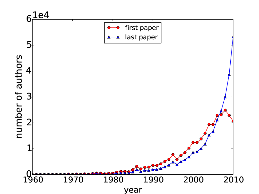
Figure 2: Start and End years.

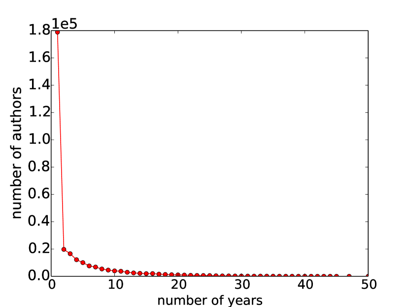
Figure 3: Research Period Length.

We use two metrics to understand the career trajectory of each researcher: burst speed and half year speed.

Definition 2 (Burst Speed)

Given an author $a$, the burst speed is defined as the number of years to reach her/his first bursty year. The bursty year is the year that with largest productive score, which is calculated as

$$v_{a}(t)=\textstyle\frac{|P_{a}(t)|}{|P_{a}|}-\frac{1}{w_{a}}$$

where $w_{a}$ is the length of research period for the author $a$, and $\mathcal{P}_{a}(t)$ is the set of papers by the author $a$ at the year $t$.

Definition 3 (Half-Speed)

Given an author $a$, the half-speed is defined as the least number of years she/he took to reach half of her/his total publications, which is calculated as:

$$h_{a}=\min_{n}\{n:\textstyle{\frac{\sum_{s=1}^{n}|P_{a}(t_{a,s})|}{|P_{a}|}}\geq\frac{1}{2}\}-1$$

Using these concepts, we can ask the following questions:

• Given a year $t$, how many authors are in their bursty year?

• Given an author $a$, which year is his/her bursty year?

• What is the average half-speed and burst-speed?

We select researchers whose research period length is larger or equal to 10 years. Among these researchers, the average number of publications is 13.8, average research period length is 15.83, average productive score is 0.212, the average burst speed is 6.32, the bursty year (in this data) associated with most authors is the year 2008, and the average half speed is 7.74. The result shows that authors reached half of their publications quickly after their bursty year. Figure 4 shows the distribution of burst speed and half speed. We observed that authors with zero half speed and burst speed account for 9.5%, and 35% of all selected authors respectively. In addition, many authors published most papers in their first year (recall, these are authors who are active for over a ten year period).

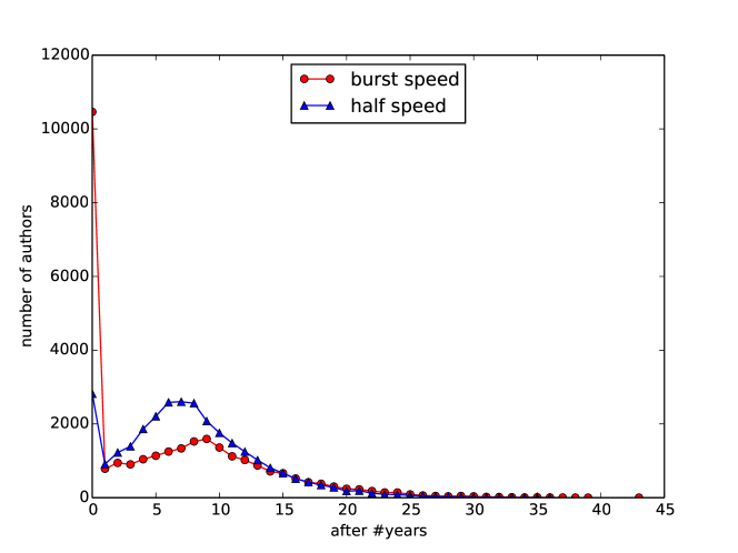
Figure 4: Burst Speed and Half Speed

We now show the correlation between the number of publications and the above definitions: research period length, burst speed and half speed. For each author with a research period of over ten years, we count the number of publications associated with her/him, find the research period length, and compute the burst and half speed. Then we take the average of research period length, burst and half speed, given a value $x$ of number of publications. Figure 5 tells that for authors who have $x$ publications, what are their average research period length, burst speed and half speed. We set a threshold of $120$ publications in the plot because there are too few points above the threshold. The figure shows logarithmic-like behavior.

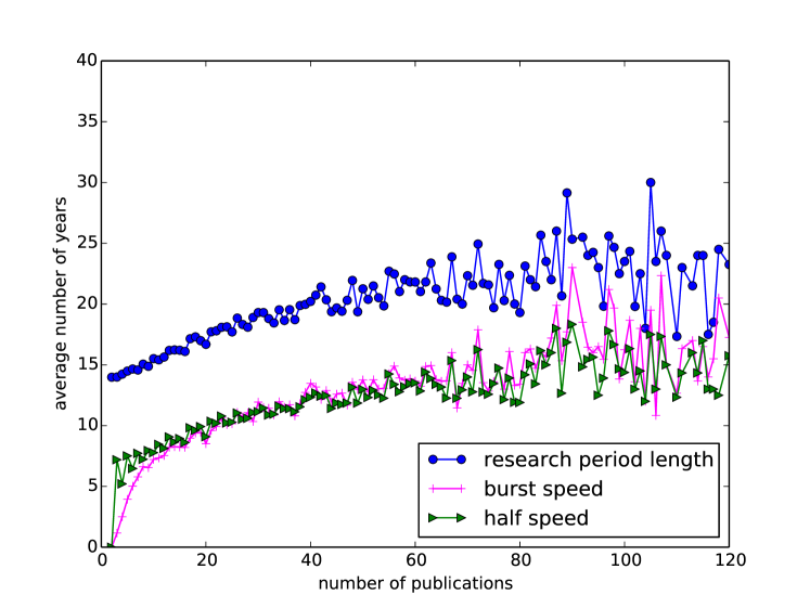
Figure 5: Correlations with # Publications

3 Evaluation and Comparison

We now describe how we define measures to evaluate and compare researchers. As mentioned above, we use venue ranking as a basis by which to evaluate a researcher. During the research period, the author publishes papers year by year, thus forming a sequence of publications, which are associated with various attributes (venue, title, abstract etc.). Table 2 shows an example of sequences, where $T(a)$ is the time sequence, $P(a)$ are publications and $V(a)$ gives venues of publication. The unit of time sequence is year, and publications and venues are ordered according to the time sequence.

Table 2: Sequence example of a researcher

Time	T(a)	$t_{a,1}$	$t_{a,2}$	$\ldots$	$t_{a,n}$
Papers	P(a)	$p_{a,1}$	$p_{a,2}$	$\ldots$	$p_{a,n}$
Venues	V(a)	$v_{a,1}$	$v_{a,2}$	$\ldots$	$v_{a,n}$

We use an existing ranking of broadly known conferences across sub-fields in computer science. This CORE ranking covers $1006$ conferences, while DBLP lists $4000$ unique conference names. The fraction of papers published in the ranked conferences is 44%. So while there is missing data, the coverage is still satisfying. Future work is to obtain a ranking that covers more venues.

The CORE ranking breaks venues into five categories: $\{$A+, A, B, C, L$\}$, where A+ is the best. We map these five categories to integer scores: $\{5,4,3,2,1\}$, in the way that ‘A+’ matches ‘5’ to ‘L’ matches ‘1’. We consider two approaches to using venue scores:

Definition 4 ( Venue Score: Categorical )

This approach treats the score as a categorical variable, which takes values from the set $\{5,4,3,2,1\}$. There is no order between two scores. The relationship between two venue scores are equal and non-equal.

Definition 5 (Venue Score: Ordinal )

In this case, score is a ordinal variable, taking values from the set $\{5,4,3,2,1\}$. The order of the venue score is determined by the integer value of the score.

3.1 On Venue Score

A key question is whether the venue score is a suitable measure on which to rank authors. We compare against two broadly accepted existing metrics: h-index and g-index, and collect values of these two metrics for authors in our corpus. We define an evaluation metric for researchers solely based on the venue score as follows.

Definition 6 (v-index)

Given a researcher $a$, the v-index is the sum of the (ordinal) venue scores of all publications by her/him.

$$\text{v-index}=\textstyle{\sum_{i=1}^{n}}v_{a,i}.$$

in which $n$ is the number of publications by the author.

Among all users in our database, the minimum of v-index is $2$, the maximum is $1229$, the mean is $53.12$ and the median is $32$. Large values on v-index only occur few times in our corpus. We compute the distribution of v-index as a function of h-index and g-index. Figure 6 shows the results. For clear visualization, we plot instances with v-index less than or equal to $800$, which covers most researchers. The $x$-axis lists each value of v-index, and the $y$-axis shows the average value of h-index or g-index given the $x$. We found for most cases, v-index has positive linear correlation with h-index and g-index. Outliers appear at very large values in each index. We conclude that venue score is an acceptable metric by which to evaluate a researcher’s research output.

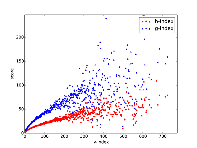
Figure 6: Correlations with h-index and g-index

Given a sequence of venue scores for each author $V(a)$, we compute the distance between two authors by matching the two sequences. This is computed with the well-known Wagner-Fischer dynamic programing algorithm [10]. We discuss how to apply the algorithm in our setting.

Given two sequences $S=s_{1}s_{2}\ldots s_{n}$ and $R=r_{1}r_{2}\ldots r_{m}$ over the alphabet $\Sigma$, the matching score between a pair $(s_{i},r_{j})$, where $s_{i},r_{j}\in\Sigma\cup\{-\}$, is as follows:

$$d(s_{i},r_{j})=\begin{cases}0,&\text{if }s_{i}=r_{j}\\ 1,&\text{if }s_{i}\neq r_{j}\\ 1,&\text{if }s_{i}=-\text{ or }r_{j}=-\end{cases}$$

The symbol “$-$” means a gap for insertion or deletion in the alignment. Dynamic programming is used to compute the optimal alignment of two sequences.

$$D(i,j)=\min\begin{cases}D(i-1,j-1)+d(s_{i},r_{j})&\text{ match or mismatch }\\ D(i-1,j)+d(s_{i},-),&\text{ insertion}\\ D(i,j-1)+d(-,r_{j}),&\text{ deletion }\end{cases}$$

where $D(i,0)=i$ and $D(0,j)=j$. In the end, $D(n,m)$ returns the minimum number operations needed to match these two sequences. A direct application of the algorithm is to treat venue score as categorical variable. Table 3 shows an example of two researchers’ sequences and their distance, where $D(a_{i},a_{j})=2$.

Table 3: An optimal sequence matching

S = $V(a_{i})$	5	4	4	3	4
R = $V(a_{j})$	5	4	5	-	4
$d$	0	0	1	1	0

It is likely that an author publishes more than one paper a year. Within a year, we can either randomly order the papers, or apply an ordering of the venue scores to form the sequence. A more sophisticated approach is considering sequences of sets rather than points. Then the distance of two positions in two sequences can be computed by the jaccard distance of sets. That is, $d(s_{i},r_{j})=1-|s_{i}\cap r_{j}|/|s_{i}\cup r_{j}|$, where $s_{i}$ is the set of publications in $i-$th year in the sequence $S$, and $r_{j}$ is the set in $j-$th year in the sequence $R$. For insertion and deletion operations, the empty set $\emptyset$ is used for the gap. The resulting distance is used to define the comparable relation between researchers:

Definition 7 (Comparable Relation)

Given a researcher $a$, and the distance between $a$ and other authors, we sort authors by the distance in ascending order. We say that the top $k$ authors are comparable to the given researcher $a$.

We experiment this approach on our corpus with authors whose research period is larger than 10 years. We sort venue scores in descending order within a year, compose a sequence of venue scores for each author, and compute the distance between each pair following by our algorithm. With distances to every other researcher computed, we determine comparable authors for any given researcher by above definition. Here we set the threshold $k$ to be $20$. For brevity, we show results of two examples and their comparable people in the Table 4. The first example is for the researcher “Judea Pearl”, who mainly focuses on research in machine learning and artificial intelligence. It is perhaps surprising that our approach returns many researchers in the same or related research areas. On the other hand, for the researcher “Dimitris N. Metaxas”, who works on compute vision, the results we returned contain researchers in various topics, for example, “Kunle Olukotun” is a pioneer of multi-core processors. Among all researchers, the average distance to their comparable authors is $16.51\pm 11.38$, the minimum is $11.12$ and maximum is $268.13$.

Table 4: Case Study of Edit Distance

Researcher	Top 20 Comparable Researchers	Average Distance
Judea Pearl	Craig Boutilier, Surajit Chaudhuri, Manfred K. Warmuth, Satinder P. Singh, Yoram Singer, Michael J. Kearns, Eyal Kushilevitz, Geoffrey E. Hinton, Silvio Micali, Avrim Blum, Shafi Goldwasser, Robert E. Schapire, Piotr Indyk, Daniel S. Weld, Andrew W. Moore, Stuart J. Russell, Jon M. Kleinberg, Jeffrey D. Ullman, Eric Horvitz, Nick Koudas	16.2
Dimitris N. Metaxas	Kunle Olukotun, Ken Kennedy, James R. Larus, Orna Grumberg, Ji-Rong Wen, A. Prasad Sistla, William T. Freeman, Richard Szeliski, Xiaolin Wu, Uzi Vishkin , Yiming Yang,Thomas G. Dietterich, Stefano Soatto, Dean M. Tullsen, Hwee Tou Ng, Christopher D. Manning, Vijay V. Vazirani, John Riedl, Robert Morris, E. Allen Emerson	21.25

3.2 On Topic Similarity

Although our corpus is focused on computer scientists, the computer science discipline spans a range of topics from theoretical studies of algorithms to computing systems in hardware and software. For real world applications, it is more common to compare researchers who work on the same or similar areas. When the pool of candidates is filtered before the evaluation and comparison, our method can be directly applied. If such prior information is not available, we propose to learn topic interests of researchers then compare them automatically. In other words, we can detect both similar and comparable people simultaneously. Our main intuition is that the matching distance of two points in two sequences can depend on both venue score and topic similarity.

We design a new distance metric to integrate both topic similarity and venue quality. Given two sequences $S$ and $R$ corresponding to authors $a_{S}$ and $a_{R}$, the matching between $i$-th point in $S$ and $j$-th point in $R$ is calculated as

$$d(s_{i},r_{j})=|v_{i}-v_{j}+\epsilon|\cdot w(p_{i},p_{j})$$

where $v_{i}$ and $p_{i}$ are $i$-th venue score and paper for author $a_{S}$; $v_{j}$ and $p_{j}$ are the corresponding venue score and paper for author $a_{R}$ (with venue score as an ordinal variable); and $\epsilon$ is a small constant, discussed below. The topic distance $w(p_{i},p_{j})$ depends on the topic similarity of two papers $p_{i}$ and $p_{j}$, and is computed as $w(p_{i},p_{j})=1-\operatorname{sim}(p_{i},p_{j})$. The value of topic similarity of two papers $\operatorname{sim}(p_{i},p_{j})$ is in [0,1]. If two papers are on similar topics, the topic distance is small, otherwise it is big.

When venue scores $v_{i},v_{j}$ are the same, in the previous algorithm, the distance is zero. However the topic distance might be large. We introduce the constant $\epsilon$ to include the topic distance for points with same venue score. In our experiments, $\epsilon$ is set to be $0.1$. Based on the above definition, we see if the topic distance is small and the venue score distance is small, the distance between these two points is small.

The topic similarity between two papers is computed based on the content of papers. In our corpus, we have the title for all papers, and abstracts for about a third of papers. To discover topics for papers, we implement Latent Dirichlet Allocation (LDA) [5]. We treat the concatenation of title and abstract of a paper as a document. Topics are derived from the whole corpus. We then obtain the topic distribution for each paper. The main parameter is the number of topics. We experimented with 20, 50 and 100 topics, with manual validation on frequent words in each topic, and select the number of topics which provides the best presentation of topics.

Table 5: Case Study of Topic Edit Distance

Topic	Researcher	Top 20 Comparable Researchers
Theory	Richard M. Karp	David R. Karger, Ravi Kumar, Jeffrey D. Ullman, Avrim Blum, Joseph Naor, Frank Thomson Leighton, Rajeev Motwani, Hari Balakrishnan, Eric Horvitz, Mostafa H. Ammar, Rina Dechter, Prabhakar Raghavan, Craig Boutilier, Rafail Ostrovsky, Raghu Ramakrishnan, Yossi Azar, James F. Kurose, Josep Torrellas, Rakesh Agrawal, Andrew Y. Ng
Machine Learning	Judea Pearl	Craig Boutilier, Satinder P. Singh, Avrim Blum, Manfred K. Warmuth, Michael J. Kearns, Piotr Indyk, Eyal Kushilevitz, Surajit Chaudhuri, Yoram Singer, Robert E. Schapire, Jon M. Kleinberg, Shafi Goldwasser, Robert Endre Tarjan, Geoffrey E. Hinton, Eric Horvitz, Milind Tambe, Jeffrey S. Rosenschein, Silvio Micali, Daniel S. Weld, Nick Koudas
Networks	Hari Balakrishnan	Ion Stoica, James F. Kurose, Baochun Li, Gustavo Alonso, Mostafa H. Ammar, Eitan Altman, Robert Endre Tarjan, Surajit Chaudhuri, Jon M. Kleinberg, Ness B. Shroff, Yossi Azar, Eli Upfal, Peter Steenkiste, Joseph Naor, Sang Hyuk Son, Qian Zhang, Frank Thomson Leighton, Randy H. Katz, Hagit Attiya, Wang-Chien Lee
Distributed Computing	Nancy Lynch	Baruch Awerbuch, Scott Shenker, J. J. Garcia-Luna-Aceves, Sajal K. Das, Roger Wattenhofer, Moni Naor, Hossam S. Hassanein, Rachid Guerraoui, Amr El Abbadi, David E. Culler, Yishay Mansour, Christos H. Papadimitriou, Klara Nahrstedt, Danny Dolev, Christos Faloutsos, Deborah Estrin, Mostafa H. Ammar, Mario Gerla, Lionel M. Ni, Serge Abiteboul
Computer Vision	Dimitris N. Metaxas	Andrew Blake, Trevor Darrell, Jitendra Malik, Jean Ponce, Narendra Ahuja, Shaogang Gong, Dale Schuurmans, Stefano Soatto, Alan L. Yuille, Pascal Fua, Aly A. Farag, Pedro Domingos, Shree K. Nayar, Xilin Chen, Chris H. Q. Ding, Brendan J. Frey, Pietro Perona, Santosh Vempala, Thomas G. Dietterich, Nassir Navab
Secrity	Dan Boneh	Amit Sahai, Ueli M. Maurer, Jacques Stern, Ronald L. Rivest, Ran Canetti, Shafi Goldwasser, Stuart J. Russell, Abraham Silberschatz, Matthew Andrews, George Varghese, Russell Impagliazzo, Cynthia Dwork, David Heckerman, Hector J. Levesque, Eyal Kushilevitz, Michael J. Kearns, Robert E. Schapire, Joe Kilian, Anoop Gupta, Tatsuaki Okamoto
Algorithms	Donald E. Knuth	Mark Roberts, H. Ramesh, Fady Alajaji, Hemant Kanakia, Mary E. S. Loomis, Michael D. Grossberg, Antonio Piccolboni, Paul Milgram, Andy Boucher, Paul Hart, Kazuo Sumita, Nicholas Carriero, Shiro Ikeda, James M. Stichnoth, Michael Bedford Taylor, Kimiko Ryokai, Riccardo Melen, Jatin Chhugani, Dianne P. O’Leary, Lal George

Given the topic distribution for each paper, we can compute the topic similarity via cosine similarity, or Jensen-Shannon divergence, etc. We use cosine similarity in our examples. With the new distance metric, the dynamic programming formula is modified to the following.

$$D(i,j)=\min\begin{cases}D(i-1,j-1)+d(s_{i},r_{j})&\text{ match or mismatch }\\ D(i-1,j)+v(s_{i}),&\text{ insertion}\\ D(i,j-1)+v(r_{j}),&\text{ deletion }\end{cases}$$

We present some examples of researchers from different topics in our results in Table 5. In general, we found results for each researcher are closer in research topics. See, for example, the output for “Dimitris N. Metaxas” in Tables 4 and 5. For “Judea Pearl”, both edit distance and topic edit distance return comparable authors in similar research topics. Recall that the topic distribution of each author is learned mostly from their paper titles. We manually validated many examples, and compared the results by simply utilizing the topic similarity between authors and by our approach. We found that sequence matching combining topics from title and venue scores did a better job in finding authors in similar research area. Taking “Richard M. Karp” for example, we find that 16 of the 20 comparable researchers returned also have entries in Wikipedia, a crude indication that they are similarly notable. Future work may more systematically examine the performance of clustering similar authors by our distance metric.

There are a few notable bad examples: the comparable researchers for “Donald E. Knuth” are only loosely related. Knuth’s paper titles are often short, and commonly use generic computer science terms like “Algorithm”. Hence, topic inference on his papers has poor performance, and the comparable authors are mainly determined on venue score sequence matching. As our data contains only $30,000$ authors, many are missing (along with their papers), limiting the set of potential comparable authors.

3.3 On Prefix Matching

Each year, many junior researchers begin their career. It is useful and interesting to matching junior researchers to segments of senior researchers. With simple modification, our algorithm can be used to compare a junior researcher to senior researchers in their early career stage. This can be useful, for example, to committees considering the future prospects of job candidates, and to junior researchers finding out whose career trajectory they are following.

Formally, we are interested in the problem that, given a senior researcher and a junior researcher characterized by $S$ and $R$ respectively. Instead of matching full sequence of $S$ and $R$, we want to match $R$ to every prefix of $S$. A prefix of the sequence $S$ with length $n$ is denoted by $S[1:k]$ where $1\leq k\leq n$. The final distance is then the minimal of matching distances with every prefix. If we store all intermediate steps of the dynamic programming table, we can easily compute the distance of prefix matching. Specifically, the vector $D(:,m)$ stores the minimal distance from every prefix of $S$ to $R$, where $m$ is the length of $R$. Consequently the minimal distance is no longer $D(n,m)$ but $\min D(:,m)$.

We sample authors with fewer than 100 papers within less than 20 years of research period to test the prefix matching. For brevity, we omit examples. Comparing to matching full sequence, there are more senior researchers mixed in the results by prefix matching.

4 Conclusions and Future Work

In this paper, we address the novel problem of automatically finding comparable researchers through large scholarly data. Unlike existing work, which evaluates researchers mainly by citation counts, our methods consider the sequence of the quality of publishing venues, which seems more appropriate for evaluating and comparing research output. To allow automatic identification of comparable people in similar research areas, we further propose a distance metric which combines the topic similarity and venue quality. Our approach can be easily modified to match junior researches to senior researcher at their beginning of research periods.

Our analysis and experiment was conducted on large-scale scholarly datasets available on the web. The effectiveness of our methods are demonstrated by arbitrarily picked examples. There are several problems open for future study.

• Data Collection: Lack of data may lead to less accurate results. Many challenges exist in the data collection, e.g. reducing the language gap, knowledge extraction from multiple data sources with different formats.

• Evaluation: There is currently no “ground truth” for our methods. We are developing a user interface to allow exploration of comparable people, and collect user feedback on results.

• Optimization: Our methods compute the matching distance between each pair of researchers through their full publication records, a quadratic number of comparisons. A different approach is required to make this more scalable.

• Comparable Network: With comparable relation established, we can define a comparable network, in which each node is a researcher, and edges connect comparable nodes. The weight on the edge is related to the distance between two nodes. It may be interesting to examine the structure of such network, and compare it with co-authorship and citation networks.

5 Acknowledgement

This work was sponsored by the NSF Grant 1161151: AF: Sparse Approximation: Theory and Extensions.

References

- [1] G. Cormode, S. Muthukrishnan, and J. Yan. Scienceography: the study of how science is written. In Fun with Algorithms, pages 379–391. Springer, 2012.
- [2] L. Egghe. An improvement of the h-index: The g-index. ISSI newsletter, 2(1), 2006.
- [3] E. Garfield. Citation analysis as a tool in journal evaluation. American Association for the Advancement of Science, 1972.
- [4] J. E. Hirsch. An index to quantify an individual’s scientific research output. PNAS, 102(46), 2005.
- [5] M. Hoffman, F. R. Bach, and D. M. Blei. Online learning for latent dirichlet allocation. In NIPS, pages 856–864, 2010.
- [6] J. Leskovec, K. J. Lang, and M. Mahoney. Empirical comparison of algorithms for network community detection. In ACM WWW, pages 631–640, 2010.
- [7] L. I. Meho. The rise and rise of citation analysis. Physics World, 2006.
- [8] M. E. Newman. Coauthorship networks and patterns of scientific collaboration. PNAS, 101:5200–5205, 2004.
- [9] J. Tang, J. Zhang, L. Yao, J. Li, L. Zhang, and Z. Su. Arnetminer: extraction and mining of academic social networks. In ACM SIGKDD, pages 990–998, 2008.
- [10] R. A. Wagner and M. J. Fischer. The string-to-string correction problem. Journal of the ACM (JACM), 21(1), 1974.