Magnetic structure of the conductive triangular-lattice antiferromagnet PdCrO₂

Abstract

We performed neutron single crystal and synchrotron X-ray powder diffraction experiments in order to investigate the magnetic and crystal structures of the conductive layered triangular-lattice antiferromagnet PdCrO₂ with a putative spin chirality, which contributes to an unconventional anomalous Hall effect. We revealed that the ground-state magnetic structure is a commensurate and nearly-coplanar 120^∘ spin structure. The 120^∘ plane in different Cr layers seem to tilt with one another, leading to a small non-coplanarity. Such a small but finite non-coplanar stacking of the 120^∘ planes gives rise to a finite scalar spin chirality, which may be responsible for the unconventional nature of the Hall effect of PdCrO₂.

I Introduction

Recently, there has been a rapid progress in the study of novel magneto-electric phenomena, such as magnetic multiferroics and unconventional anomalous Hall effect (UAHE) Nagaosa et al. (2010); Xiao et al. (2010); Tokura and Seki (2010); Arima (2011). Common to all of these is that they involve a spin current, i.e., magnetic structures with spin chiralities. In case of UAHE, a topological quantum effect has been proposed as a potential mechanism Nagaosa et al. (2010); Xiao et al. (2010): In a magnetic structure with the scalar spin chirality $\chi_{ijk}=\bm{S}_{i}\cdot(\bm{S}_{j}\times\bm{S}_{k})$, the wave function of a conduction electron gains a Berry phase, which plays a role of a fictitious magnetic field and leads to appearance of the Hall voltage even without the net magnetization. The magnitude of the fictitious field is proportional to the solid angle formed by the three non-coplanar spins Taguchi et al. (2001); Yasui et al. (2006); Machida et al. (2007, 2009); Matl et al. (1998); Ye et al. (1999); Ohgushi et al. (2000); Tatara and Kawamura (2002); Tomizawa and Kontani (2009); Taguchi and Tatara (2009). This mechanism is in analogy to the Aharonov-Bohm effect Aharonov and Bohm (1959).

In search of UAHE attributable to the spin chirality, geometrically frustrated magnets are particularly promising, because they often exhibit non-coplanar spin configurations with finite spin chiralities. Indeed, the UAHE has been observed in materials with structures that are three-dimensional analogues of the triangular lattice (TL) Taguchi et al. (2001); Yasui et al. (2006); Machida et al. (2007, 2009); Matl et al. (1998). However, in two dimensional (2D) TL systems, which is the simplest example of a geometrically frustrated spin system, the UAHE has been observed only recently Takatsu et al. (2010); Shiomi et al. (2012). Naively, the UAHE driven by the Berry-phase concept cannot be expected in a coplanar 120^∘ spin structure, which is often realized in 2D-TL antiferromagnets. This is because $\chi_{ijk}$ is locally zero for every triangles or, even if $\chi_{ijk}$ is locally finite, the net chirality vanishes because $\chi_{ijk}$ of different triangles cancels out Nagaosa et al. (2010); Tatara and Kawamura (2002). However, $\chi_{ijk}$ may remain finite, if the spin chirality and magnetization are coupled with the help of the spin-orbit interaction Tatara and Kawamura (2002); Kawamura (2003), or in non-coplanar spin structures with a four-site magnetic unit cell Shindou and Nagaosa (2001); Martin and Batista (2008); Akagi and Motome (2010), both of which change the balance of the uniform $\chi_{ijk}$ on each triangle. The fundamental mechanism for the UAHE observed in the frustrated 2D-TL systems is thus not well understood and is awaited to be clarified.

The delafossite compound PdCrO₂ is a rare example of a 2D-TL antiferromagnet that exhibits UAHE Takatsu et al. (2010). The metallic conduction of this material is predominantly attributed to the Pd $4d$ electron band Ok et al. (2013); Sobota et al. (2013); Ong and Singh (2012), and the magnetic properties are governed by the localized spins of Cr³⁺ ions ($S=3/2$), which order antiferromagnetically at $T_{\mathrm{N}}=37.5$ K Doumerc et al. (1986); Mekata et al. (1995); Takatsu et al. (2009). The spin Hamiltonian of this system is approximately written as

$$H=-2J\sum_{<i,j>}\bm{S}_{i}\cdot\bm{S}_{j}-2J^{\prime}\sum_{<l,m>}\bm{S}_{l}\cdot\bm{S}_{m}+D\sum_{i}(S_{i}^{z})^{2},$$ (1)

where $J(<0)$ and $J^{\prime}$ are the nearest-neighbor intraplane and interplane interactions, respectively, and $D$ is the single ion anisotropy. The anisotropy of the magnetic susceptibility $\chi$, associated with a sharp drop in $\chi_{c}$ below $T_{\mathrm{N}}$, strongly suggests an easy-axis anisotropy along the $z$ axis, $D<0$ Ong and Singh (2012); Hirone and Adachi (1957). Remarkably, this material exhibits UAHE below $T^{*}\simeq 20$ K, noticeably lower than $T_{\mathrm{N}}$ Takatsu et al. (2010): The Hall resistivity $\rho_{xy}$ exhibits an unusual non-linear field dependence. Apparently it deviates from the conventional behavior that is a linear function of both magnetic induction and magnetization Hurd (1972), since the magnetization of PdCrO₂ is proportional to $H$ down to 2 K Takatsu et al. (2010). We expect that a non-coplanar spin structure with a finite spin chirality probably plays a crucial role for the emergence of the UAHE in this compound.

In this study, we have performed neutron scattering experiments on a single crystalline sample of PdCrO₂ to determine the magnetic structure in zero magnetic field. We found that it is a commensurate 120^∘ spin structure, and that a small change of the magnetic structure occurs around $T^{*}$. The magnetic structure analysis suggests alternative stacking of 120^∘ spin layers, which seems to be tilt with one another. We thus identify a non-coplanar 120^∘ spin structure as the probable origin of the UAHE, because the scalar spin chirality mechanism will work in this structure in the presence of a net magnetization induced by an external magnetic field.

II Experimental

Single crystals of PdCrO₂ were grown by a NaCl flux using PdCrO₂ powder synthesized via a solid state reaction Takatsu and Maeno (2010). Synchrotron X-ray powder diffraction experiments were performed on the BL02B2 beam line at SPring-8 from 300 K to 11 K. We used a powder sample prepared by crushing single crystals. The powder was packed into a glass tube ($\phi=0.1$ mm) and mounted into a closed-cycle ⁴He-gas refrigerator. The wavelength of the incident beam was $\lambda=0.6$ Å. A homogeneous granularity of the sample was checked by a homogeneous intensity distribution in the Debye-Scherrer diffraction rings.

Neutron single-crystal diffraction experiments were performed with the triple-axis spectrometers 4G and C11 installed at the research reactor JRR-3M at Japan Atomic Energy Agency. The neutron wavelength was fixed at either $\lambda=1.64$ or $2.35$ Å  (4G), and at $4.07$ Å  (C11). Pyrolytic graphite (PG) (002) reflections were used as both monochromator and analyzer. Higher-order neutrons were removed by a PG-filter or a Be-filter. We employed collimations 20’-20’-20’-20’ (4G) or 20’-20’-open (C11). The sample was mounted in a closed-cycle ⁴He-gas refrigerator so that the horizontal scattering plane of the spectrometer coincided with the hexagonal ($h$ $h$ $l$) or ($h$ $k$ 0) zones of the $R\bar{3}m$ symmetry. A precise determination of the crystal structure symmetry is described later. Integrated intensities of many Bragg reflections were measured with the four circle diffractometer D10 at Institute Laue-Langevin (ILL). Incident neutrons of wavelength $\lambda=2.36$ Å  monochromated by PG(002) were used. The sample was mounted in a He flow cryostat. In order to perform a detailed structural analysis, experiments were also carried out at room temperature (RT) with the hot-neutron four-circle diffractometer D9 at ILL. We used a neutron wavelength of $\lambda=0.838$ Å. In all the experiments, we used the same single crystal that has the dimensions $1.5\times 3.0\times 0.2$ mm³ with the flat plane shape along the hexagonal $ab$ plane.

III Results

III.1 Determination of the crystal structure

Figure 1: (Color online) Synchrotron X-ray diffraction patterns of PdCrO₂ measured at $T=300$ K and 11 K. Observed and refined data are shown by crosses and solid curves, respectively. The difference between the data and the model is plotted by the dashed curves in the lower part. Vertical bars represent positions of the Bragg reflections. Additional Cu peaks come from the sample holder used in the experiments. The Rietveld refinement revealed that PdCrO₂ retains to have the $R\bar{3}m$ crystal-structure symmetry down to 11 K.

Since a precise crystal structure determination of PdCrO₂ has not been reported, we have undertaken single crystal neutron and powder X-ray characterization. Figure 1 shows powder X-ray diffraction patterns taken at 300 K and 11 K. The diffraction patterns were reasonably fitted by parameters of the delafossite structure with the space group $R\bar{3}m$ for both temperatures. The $R$ factors of the Rietveld refinement Izumi and Momma (2007) were obtained as $R_{\mathrm{wp}}=4.95$%, $R_{\mathrm{e}}=3.87$%, $R_{\mathrm{p}}=3.61$%, $R_{\mathrm{B}}=4.94$% for 300 K, and $R_{\mathrm{wp}}=4.36$%, $R_{\mathrm{e}}=3.20$%, $R_{\mathrm{p}}=3.27$%, $R_{\mathrm{B}}=4.70$% for 11 K, respectively. The goodness-of-fit parameter, $S=R_{\mathrm{wp}}/R_{\mathrm{e}}$, was $S=1.28$ and 1.36 for 300 K and 11 K, respectively. Excellent refinement was also confirmed by using neutron data at D9, which achieved $\chi^{2}$ = 1.015 for 86 unique reflections. The resulting structure parameters are listed in Tables 1 and  2. These results demonstrate that PdCrO₂ remains in the $R\bar{3}m$ symmetry down to low temperatures.

Table 1: Structure parameters for PdCrO₂ refined by Rietveld analysis of the X-ray data and the neutron data from D9. The analysis was performed assuming the space group $R\bar{3}m$ with atomic positions: Pd 3a (0,0,0), Cr 3b (0,0,0.5), and O 6c (0,0,$z$). $U_{\mathrm{iso}}$ represents the isotropic atomic displacement parameter.

	x-ray(300 K)	neutron(RT)	x-ray(11 K)
Cell parameters and positions
$a$ (Å)	2.9228(2)	2.9280(1)	2.9011(3)
$c$ (Å)	18.093(1)	18.1217(9)	18.028(2)
$z$	0.1105(1)	0.11057(3)	0.1102(1)
$U_{\mathrm{iso}}$ ($10^{-3}$Å2)
Pd	5.1(1)	5.8(3)	1.8(1)
Cr	4.4(1)	4.6(3)	2.3(1)
O	4.4(3)	5.3(3)	3.7(3)

Table 2: Anisotropic atomic displacement parameters $U_{ij}$ (in units of $10^{-3}$Ų) of PdCrO₂ at RT. The parameters were refined with the neutron data from D9.

Atom	$U_{\mathrm{11}}$	$U_{\mathrm{22}}$	$U_{\mathrm{33}}$	$U_{\mathrm{12}}$	$U_{\mathrm{13}}$	$U_{\mathrm{23}}$
Pd	6.2(3)	6.2(3)	4.9(3)	3.1(3)	0	0
Cr	4.1(3)	4.1(3)	5.5(3)	2.0(3)	0	0
O	5.2(3)	5.2(3)	5.4(2)	2.6(3)	0	0

III.2 Neutron diffraction

Magnetic reflections of PdCrO₂ were observed at $\bm{Q}=(\frac{1}{3},\frac{1}{3},l)$ and ($\frac{2}{3},\frac{2}{3},l$) with $l=0,\frac{1}{2},1,\frac{3}{2},2\cdots$, being consistent with the previous reports of powder neutron diffraction Mekata et al. (1995); Takatsu et al. (2009). We confirmed that those magnetic peaks appear at commensurate positions within the present experimental accuracies of the 4G and C11 spectrometers. We did not find any magnetic reflections at $\bm{Q}=(00l)$, $(10l)$, $(01l)$,$(11l)$ with $l=0,\frac{1}{2},1,\frac{3}{2},\cdots$. Figure 2 shows the temperature dependence of intensities of the magnetic reflections at ($\frac{1}{3},\frac{1}{3},0$) and ($\frac{1}{3},\frac{1}{3},\frac{7}{2}$). The magnetic peaks appear at temperatures below $T_{\mathrm{N}}$ and their intensities monotonically increase on cooling. Two successive phase transitions, separated by $\varDelta T=0.4$ K, are observed in the specific heat data not . These transitions are expected for a small finite $D$ ($<0$) Fujiki et al. (1983); Blankschtein et al. (1984); Kimura et al. (2008). However, such splitting of $T_{\mathrm{N}}$ could not be detected in the neutron diffraction experiment within the experimental accuracy of 1 K. This small split of $T_{\mathrm{N}}$ will have to be confirmed by diffraction experiments in future. The intensity ratio between ($\frac{1}{3},\frac{1}{3},0$) and ($\frac{1}{3},\frac{1}{3},\frac{7}{2}$) reflections is still slightly temperature dependent below about 20–30 K (the inset of Fig. 2). This feature is also confirmed by intensity ratios of magnetic reflections taken at 2 K and 30 K (Fig. 3). These results imply that a slight change of magnetic structure occurs around $T^{*}\sim 20$ K, which is in accord with the appearance of UAHE below this temperature.

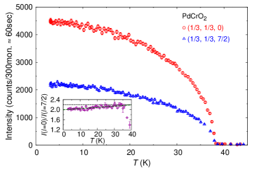
Figure 2: (Color online) Temperature dependence of the intensity $I(l)$ of magnetic reflections at (1/3, 1/3, $l$) with $l=0$ and $\frac{7}{2}$. The inset shows the temperature dependence of the intensity ratio $I(l=0)/I(l=\frac{7}{2})$. The deviation from the constant value for its ratio below $T_{\rm N}$ suggests that a slight change in the spin configuration appears at temperatures below 30 K.

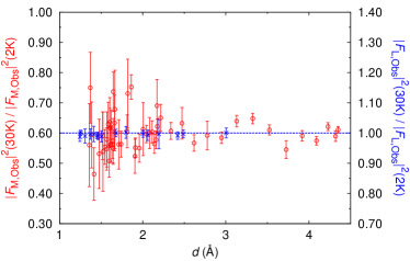
Figure 3: (Color online) Intensity ratios of magnetic or nuclear reflections taken at 30 and 2 K. The graph is plotted for the ratios vs the distance between lattice planes, $d$. The ratio of nuclear reflections ($|F_{\mathrm{L,Obs}}|^{2}(30\mathrm{K})/|F_{\mathrm{L,Obs}}|^{2}(2\mathrm{K})$) is constant, while that of magnetic reflections ($|F_{\mathrm{M,Obs}}|^{2}(30\mathrm{K})/|F_{\mathrm{M,Obs}}|^{2}(2\mathrm{K})$) deviates from a constant value. This result also suggests appearance of a small difference in the magnetic structure between 30 K and 2 K.

To analyze the magnetic and crystal structures, we measured integrated intensities of the Bragg reflections at 2 K and 30 K with the four circle spectrometer D10. Observed and calculated squares of the structure factor of nuclear reflections are listed in Table I of the Supplemental Material sup . For the calculation, we assumed the delafossite structure and refined one parameter of the oxygen-ion position $z$. We obtained $z=0.1104(1)$, which agrees well with results given in Table 1. Due to the secondary extinction effect, the observed values for the larger intensities tend to deviate from the calculated values, while those for the smaller intensities are in agreement with calculations (Fig. 4).

III.3 Magnetic structure analysis

In order to fit the integrated intensities of the magnetic reflections, we considered four structure models for the magnetic structure. All of these consist of spins that lie in a plane containing the hexagonal $c$ axis: (1) the coplanar single-$q$ 120^∘ spin structure, where the integer $l$ and half-integer $l$ reflections come from different $q$ modulation domains [Fig. 5 (a)]; (2) a single-$q$ structure with a collinear polarization, which also forms multiple domains [Fig. 5 (b)]; (3) a general multi-$q$ coplanar 120^∘ spin structure, which has a clockwise (+) and anticlockwise (-) rotation degree of freedom in each layer [Fig. 5 (c)]; (4) a non-coplanar spin structure based on the general 120^∘ spin structure of the model (3), where now the spin plane can rotate around the $c$ axis from one $z$-layer to the next [Fig. 5 (d)]. This rotational misfit is characterized by the normal vector to the 120^∘-spin plane, which is considered to point into different directions for each $z$-layer. The orientation of the 120^∘-spin plane can be described by different azimuthal angles of its normal vector $\alpha_{n}$ ($n=0,1,2,3,4,5$) for each layer. We performed a least-squares fit by these models and found that models (3) and (4) provide solutions that account for the observed intensities. The representation analysis revealed that these magnetic structures can be classified by using small representations deduced from the $R\bar{3}m$ crystal symmetry (Sect. III.3.6 and Appendix). The details of analysis are as follows.

The intensity of the magnetic reflection at a wave vector $\bm{Q}$ is written as

$$I=(\gamma r_{0})^{2}|F_{\mathrm{M}}(\bm{Q})|^{2}\Bigl{[}\frac{g}{2}f(\bm{Q})\Bigr{]}^{2},$$ (2)

$$F_{\mathrm{M}}(\bm{Q})=\sum_{\begin{subarray}{c}\mathrm{\ magnetic}\\ \mathrm{unit\,cell}\end{subarray}}\exp({i\bm{Q}\cdot\bm{R}})\bigr{[}\bm{S}_{\bm{R}}-\hat{\bm{Q}}(\hat{\bm{Q}}\cdot\bm{S}_{\bm{R}})\bigl{]},$$ (3)

where $\gamma=1.913$, $r_{0}$ is the classical radius of the electron, $g$ and $f(\bm{Q})$ are the $g$ factor and magnetic form factor of Cr³⁺, respectively. Here, we assumed $g\simeq 2$ following the result of the electron spin resonance spectroscopy Hemmeida et al. (2011). $\hat{\bm{Q}}$ is the unit vector along the wave-vector transfer $\bm{Q}$. In Eq. (2), the temperature factor is neglected. For the analysis, we have taken an average of $|F_{\mathrm{M}}(\bm{Q})|^{2}$ over magnetic structure domains, which are naturally derived by symmetry operations of the space group $R\bar{3}m$.

Magnetic structure models of PdCrO₂ that we consider consist of 18 sublattice structures, whose 18 magnetic Cr sites A_n, B_n, and C_n ($n=0,1,2,3,4,5$) are shown in Fig. 5(e). The hexagonal coordinates of the sublattice sites $\bm{R}_{\text{A}_{n}}$, $\bm{R}_{\text{B}_{n}}$, and $\bm{R}_{\text{C}_{n}}$ are

$$\bm{R}_{\text{A}_{0}} =\left(0,0,\frac{1}{2}\right),\bm{R}_{\text{A}_{1}}=\left(\frac{2}{3},\frac{1}{3},\frac{5}{6}\right),\bm{R}_{\text{A}_{2}}=\left(\frac{4}{3},\frac{2}{3},\frac{7}{6}\right)$$

$$\bm{R}_{\text{A}_{3}} =\left(0,0,\frac{3}{2}\right),\bm{R}_{\text{A}_{4}}=\left(\frac{2}{3},\frac{1}{3},\frac{11}{6}\right),\bm{R}_{\text{A}_{5}}=\left(\frac{4}{3},\frac{2}{3},\frac{13}{6}\right)$$

$$\bm{R}_{\text{B}_{n}} =\bm{R}_{\text{A}_{n}}+(1,0,0),$$

$$\bm{R}_{\text{C}_{n}} =\bm{R}_{\text{A}_{n}}+(2,0,0).$$

The observation of no magnetic intensity at reflections $\bm{Q}=(00l)$, $(10l)$, $(01l)$, $(11l)$ with $l=0,\frac{1}{2},1,\frac{3}{2},\cdots$ indicates that the 18 sublattice spins $\bm{S}_{\text{A}_{n}}$, $\bm{S}_{\text{B}_{n}}$, and $\bm{S}_{\text{C}_{n}}$ satisfy constraints

$$\bm{S}_{\text{A}_{n}}+\bm{S}_{\text{B}_{n}}+\bm{S}_{\text{C}_{n}}=0.$$ (4)

These constraints are alternatively expressed by a six-$q$ structure

$$\bm{S}_{\text{X}_{n}} =\sum_{j=1}^{6}\left(\bm{a}_{j}\exp[i\bm{q}_{j}\cdot\bm{R}_{\text{X}_{n}}]+\bm{a}_{j}^{\ast}\exp[-i\bm{q}_{j}\cdot\bm{R}_{\text{X}_{n}}]\right)$$

$$=\sum_{j=1}^{6}2\left(\bm{a}_{j}^{\prime}\cos[\bm{q}_{j}\cdot\bm{R}_{\text{X}_{n}}]+\bm{a}_{j}^{\prime\prime}\sin[\bm{q}_{j}\cdot\bm{R}_{\text{X}_{n}}]\right),$$ (5)

where $\text{X}_{n}$ stands for A_n, B_n, or C_n, and wave vectors $\bm{q}_{j}$ are

$$\bm{q}_{1} =\left(\frac{1}{3},\frac{1}{3},0\right),\bm{q}_{2}=\left(-\frac{2}{3},\frac{1}{3},0\right),\bm{q}_{3}=\left(\frac{1}{3},-\frac{2}{3},0\right),$$

$$\bm{q}_{4} =\left(\frac{1}{3},\frac{1}{3},\frac{1}{2}\right),\bm{q}_{5}=\left(-\frac{2}{3},\frac{1}{3},\frac{1}{2}\right),\bm{q}_{6}=\left(\frac{1}{3},-\frac{2}{3},\frac{1}{2}\right).$$ (6)

In Eq. (5), $\bm{a}_{j}=\bm{a}_{j}^{\prime}-i\bm{a}_{j}^{\prime\prime}$ are complex vectors, whereas $\bm{a}_{j}^{\prime}$ and $\bm{a}_{j}^{\prime\prime}$ are real vectors.

In principle there are 36 adjustable parameters for the present magnetic structure determination (12 real or 6 complex vectors), we therefore considered the simplified structure models (1)–(4) to reduce number of fitting parameters. Note that as discussed later, we confirmed that all of these magnetic structures were classified by using symmetry properties of the space group $R\bar{3}m$ of the crystal symmetry.

III.3.1 Model (1): single-$q$ 120^∘ spin structure

We assume multiple domains of a single-$q$ structure, which consists of a 120^∘ spin plane including the $c$ axis [Fig. 5(a)]. This is the simplest structure model deduced from the spin Hamiltonian of Eq. (1). The magnetic structure of one domain responsible for integer-$l$ reflections is

$$\bm{S}_{\text{X}_{n}} =S\hat{{\bm{z}}}\cos[\phi+\bm{q}_{1}\cdot\bm{R}_{\text{X}_{n}}]+S\hat{\bm{e}}_{\alpha}\sin[\phi+\bm{q}_{1}\cdot\bm{R}_{\text{X}_{n}}],$$ (7)

$$\hat{\bm{e}}_{\alpha} =\hat{{\bm{x}}}\cos\alpha+\hat{{\bm{y}}}\sin\alpha,$$

where $\hat{{\bm{x}}}$, $\hat{{\bm{y}}}$, and $\hat{{\bm{z}}}$ are orthogonal unit vectors ($\hat{{\bm{a}}}=a\hat{{\bm{x}}}$, $\hat{{\bm{b}}}=a(-\frac{1}{2}\hat{{\bm{x}}}+\frac{\sqrt{3}}{2}\hat{{\bm{y}}})$, and $\hat{{\bm{c}}}=c\hat{{\bm{z}}}$), $\alpha$ and $\phi$ are constants. Note that Eq. (7) is deduced from Eq. (5) by substituting $\bm{a}_{1}=\frac{S}{2}(\hat{{\bm{z}}}-i\hat{\bm{e}}_{\alpha})e^{i\phi}$. Each spin of this domain can be written as

$$\bm{S}_{\text{A}_{n}} =S\left[\hat{\bm{z}}\cos\phi_{1,n}+\hat{\bm{e}}_{\alpha}\sin\phi_{1,n}\right],$$

$$\bm{S}_{\text{B}_{n}} =S\left[\hat{\bm{z}}\cos\left(\phi_{1,n}+\frac{2\pi}{3}\right)+\hat{\bm{e}}_{\alpha}\sin\left(\phi_{1,n}+\frac{2\pi}{3}\right)\right],$$

$$\bm{S}_{\text{C}_{n}} =S\left[\hat{\bm{z}}\cos\left(\phi_{1,n}-\frac{2\pi}{3}\right)+\hat{\bm{e}}_{\alpha}\sin\left(\phi_{1,n}-\frac{2\pi}{3}\right)\right],$$ (8)

where $\phi_{1,n}=\phi+\frac{2\pi}{3}n$, and $\phi$ is assumed to be zero in the analysis. Symmetrically equivalent domains responsible for integer-$l$ reflections are obtained by transformations of the space group operations with respect to $\bm{q}_{1}\rightarrow\bm{q}_{j}$ ($j=2,3$).

One magnetic domain responsible for half-integer-$l$ reflections consists of the spin vectors

$$\bm{S}_{\text{X}_{n}} =S\hat{{\bm{z}}}\cos[\phi+\bm{q}_{4}\cdot\bm{R}_{\text{X}_{n}}]+S\hat{\bm{e}}_{\alpha}\sin[\phi+\bm{q}_{4}\cdot\bm{R}_{\text{X}_{n}}],$$ (9)

$$\hat{\bm{e}}_{\alpha} =\hat{{\bm{x}}}\cos\alpha+\hat{{\bm{y}}}\sin\alpha,$$

where $\alpha$ and $\phi$ are constants. Here, Eq. (9) is equivalent to Eq. (5) with $\bm{a}_{4}=\frac{S}{2}(\hat{{\bm{z}}}-i\hat{\bm{e}}_{\alpha})e^{i\phi}$, as in the case of the integer-$l$ domain. Each spin is

$$\bm{S}_{\text{A}_{n}} =S\left[\hat{\bm{z}}\cos\phi_{4,n}+\hat{\bm{e}}_{\alpha}\sin\phi_{4,n}\right],$$

$$\bm{S}_{\text{B}_{n}} =S\left[\hat{\bm{z}}\cos\left(\phi_{4,n}+\frac{2\pi}{3}\right)+\hat{\bm{e}}_{\alpha}\sin\left(\phi_{4,n}+\frac{2\pi}{3}\right)\right],$$

$$\bm{S}_{\text{C}_{n}} =S\left[\hat{\bm{z}}\cos\left(\phi_{4,n}-\frac{2\pi}{3}\right)+\hat{\bm{e}}_{\alpha}\sin\left(\phi_{4,n}-\frac{2\pi}{3}\right)\right],$$ (10)

where $\phi_{4,n}=\phi+\sigma_{n}\frac{\pi}{2}$ and $\phi$ is assumed to be zero. Here, $\sigma_{n}=(-1)^{n}$. Symmetrically equivalent domains are obtained by transformations of the space group operations with respect to $\bm{q}_{4}\rightarrow\bm{q}_{j}$ ($j=5,6$).

III.3.2 Model (2): single-$q$ collinear spin structure

We assume a single-$q$ collinear structure with multiple domains [Fig. 5(b)]. The magnetic structure of a domain, which is responsible for integer-$l$ reflections, is described by e.g.,

$$\bm{S}_{\text{X}_{n}} =\bm{a}_{1}\exp[i\bm{q}_{1}\cdot\bm{R}_{\text{X}_{n}}]+\bm{a}_{1}^{\ast}\exp[-i\bm{q}_{1}\cdot\bm{R}_{\text{X}_{n}}]$$ (11)

$$\bm{a}_{1} =\frac{1}{2}S(\cos\beta\hat{{\bm{z}}}+\sin\beta\hat{\bm{e}}_{\alpha})\exp(i\phi),$$

where $S$, $\beta$, and $\phi$ are constants. Each spin is

$$\bm{S}_{\text{A}_{n}}=S(\cos\beta\hat{{\bm{z}}}+\sin\beta\hat{\bm{e}}_{\alpha})\cos\phi_{1,n},$$

$$\bm{S}_{\text{B}_{n}}=S(\cos\beta\hat{{\bm{z}}}+\sin\beta\hat{\bm{e}}_{\alpha})\cos\left(\phi_{1,n}+\frac{2\pi}{3}\right),$$

$$\bm{S}_{\text{C}_{n}}=S(\cos\beta\hat{{\bm{z}}}+\sin\beta\hat{\bm{e}}_{\alpha})\cos\left(\phi_{1,n}-\frac{2\pi}{3}\right),$$

$$\hat{\bm{e}}_{\alpha}=\hat{{\bm{x}}}\cos\alpha+\hat{{\bm{y}}}\sin\alpha,$$

where $\phi_{1,n}=\phi+\frac{2\pi}{3}n$ ($n=0,1,2,3,4,5$) and $\phi$ is assumed to be zero. Symmetrically equivalent domains are obtained by transformations of the space group operations with respect to $\bm{q}_{1}\rightarrow\bm{q}_{j}$ ($j=2,3$).

A magnetic domain, which provides half-integer-$l$ reflections, is

$$\bm{S}_{\text{X}_{n}} =\bm{a}_{4}\exp[i\bm{q}_{4}\cdot\bm{R}_{\text{X}_{n}}]+\bm{a}_{4}^{\ast}\exp[-i\bm{q}_{4}\cdot\bm{R}_{\text{X}_{n}}]\$$ (13)

$$\bm{a}_{4} =\frac{1}{2}S(\cos\beta\hat{{\bm{z}}}+\sin\beta\hat{\bm{e}}_{\alpha})\exp(i\phi).$$

Each spin is written by

$$\bm{S}_{\text{A}_{n}}=S(\cos\beta\hat{{\bm{z}}}+\sin\beta\hat{\bm{e}}_{\alpha})\cos\phi_{4,n},$$

$$\bm{S}_{\text{B}_{n}}=S(\cos\beta\hat{{\bm{z}}}+\sin\beta\hat{\bm{e}}_{\alpha})\cos\left(\phi_{4,n}+\frac{2\pi}{3}\right),$$

$$\bm{S}_{\text{C}_{n}}=S(\cos\beta\hat{{\bm{z}}}+\sin\beta\hat{\bm{e}}_{\alpha})\cos\left(\phi_{4,n}-\frac{2\pi}{3}\right),$$

$$\hat{\bm{e}}_{\alpha}=\hat{{\bm{x}}}\cos\alpha+\hat{{\bm{y}}}\sin\alpha,$$

where $\phi_{4,n}=\phi+\sigma_{n}\frac{\pi}{2}$ and $\phi$ is assumed to be zero. Here, $\sigma_{n}=(-1)^{n}$. Symmetrically equivalent domains are obtained by transformations of the space group operations with respect to $\bm{q}_{4}\rightarrow\bm{q}_{j}$ ($j=5,6$).

III.3.3 Model (3): coplanar 120^∘ spin structure

For the model (3), we consider as before a coplanar 120^∘ spin structure in a plane parallel to the $c$ axis [Fig. 5(c)]. Each spin is now written as

$$\bm{S}_{\text{A}_{n}}=S\left[\hat{\bm{z}}\cos\phi_{n}+\hat{\bm{e}}_{\alpha}\sin\phi_{n}\right],$$

$$\bm{S}_{\text{B}_{n}}=S\left[\hat{\bm{z}}\cos\left(\phi_{n}+\xi_{n}\frac{2\pi}{3}\right)+\hat{\bm{e}}_{\alpha}\sin\left(\phi_{n}+\xi_{n}\frac{2\pi}{3}\right)\right],$$

$$\bm{S}_{\text{C}_{n}}=S\left[\hat{\bm{z}}\cos\left(\phi_{n}-\xi_{n}\frac{2\pi}{3}\right)+\hat{\bm{e}}_{\alpha}\sin\left(\phi_{n}-\xi_{n}\frac{2\pi}{3}\right)\right],$$

$$\hat{\bm{e}}_{\alpha}=\hat{{\bm{x}}}\cos\alpha+\hat{{\bm{y}}}\sin\alpha,$$

where $\phi_{n}$ ($n=0,1,2,3,4,5$) are constants, which represent rotation angles of the 120^∘ spin around the normal vector of the plane consisting of the $\hat{\bm{c}}$ and $\hat{\bm{e}}_{\alpha}$ vectors. Here we have introduced an additional degree of freedom $\xi_{n}=\pm 1$, which describes the rotation direction of spins: $\xi_{n}=+1$ represents the clockwise rotation, while $\xi_{n}=-1$ describes the anticlockwise rotation. This parameter $\xi_{n}$ allows to test 32 different structures which can be grouped into eight independent classes of spin structures, related to the rotation sense of spins in each layer, that is, $++++++$, $+++++-$, $++++--$, $+++-+-$, $++-++-$, $+++---$, $++-+--$, $+-+-+-$. Here, $+$, $-$ stand for $\xi_{n}=+1$, $-1$, respectively.

III.3.4 Model (4): non-coplanar 120^∘ spin structure

For the model (4), we consider a non-coplanar 120^∘ spin structure where the non-coplanarity of spin configurations is introduced by different orientations of the 120^∘ spin-planes in subsequent $z$-layers [Fig. 5(d)]. Spin vectors of this structure are

$$\bm{S}_{\text{A}_{n}}=S\Bigl{[}\hat{\bm{z}}\cos\gamma_{n}\cos\phi_{n}+\hat{\bm{e}}_{\alpha_{n}}\sin\phi_{n}+\hat{\bm{e}}_{\alpha_{n}^{\prime}}\sin\gamma_{n}\cos\phi_{n}\Bigr{]},$$

$$\bm{S}_{\text{B}_{n}}=S\biggl{[}\hat{\bm{z}}\cos\gamma_{n}\cos\left(\phi_{n}+\xi_{n}\frac{2\pi}{3}\right)$$

$$\hskip 5.0pt+\hat{\bm{e}}_{\alpha_{n}}\sin\left(\phi_{n}+\xi_{n}\frac{2\pi}{3}\right)+\hat{\bm{e}}_{\alpha_{n}^{\prime}}\sin\gamma_{n}\cos\left(\phi_{n}+\xi_{n}\frac{2\pi}{3}\right)\biggr{]},$$

$$\bm{S}_{\text{C}_{n}}=S\biggl{[}\hat{\bm{z}}\cos\gamma_{n}\cos\left(\phi_{n}-\xi_{n}\frac{2\pi}{3}\right)$$

$$\hskip 5.0pt+\hat{\bm{e}}_{\alpha_{n}}\sin\left(\phi_{n}-\xi_{n}\frac{2\pi}{3}\right)+\hat{\bm{e}}_{\alpha_{n}^{\prime}}\sin\gamma_{n}\cos\left(\phi_{n}-\xi_{n}\frac{2\pi}{3}\right)\biggr{]},$$

$$\hat{\bm{e}}_{\alpha_{n}}=\hat{{\bm{x}}}\cos\alpha_{n}+\hat{{\bm{y}}}\sin\alpha_{n},$$

$$\hat{\bm{e}}_{\alpha_{n}^{\prime}}=\hat{{\bm{x}}}\cos\Bigl{(}\alpha_{n}+\frac{\pi}{2}\Bigr{)}+\hat{{\bm{y}}}\sin\Bigl{(}\alpha_{n}+\frac{\pi}{2}\Bigr{)},$$ (16)

where $\gamma_{n}$, $\alpha_{n}$ and $\phi_{n}$ ($n=0,1,2,3,4,5$) are constants, indicating polar angles from the $z$ axis to the normal vector of the plane consisting of the $\hat{\bm{c}}$ and $\hat{\bm{e}}_{\alpha}$ vectors, azimuthal angles of the spin-plane normal in the different $z$-layers, and rotation angles of the 120^∘ spin around the normal vector, respectively. In the analysis, we assume that in each $z$-layer the 120^∘ plane is parallel to the $c$ axis (i.e., $\gamma_{n}=0$). We also consider a case that there is a misfit between $\alpha_{n}$ of even ($n=0,2,4$) layers and that of odd ($n=1,3,5$) layers. This structure is, however, represented by irreducible representations of the $R\bar{3}m$ crystal symmetry, which will be discussed in detail in Sect. III.3.6. In Eq. (16), the definition of $\xi_{n}$ is the same as that of the model (3). Here, we fixed $\xi_{n}$ so that $\xi_{n}=+1$ ($n=0,2,4$) and $\xi_{n}=-1$ ($n=1,3,5$). Note that we can consider other combinations in these parameters, however they do not change the general fitting result because misfit angles $\alpha_{n}$ between layers are fitting parameters, namely certain values of $\alpha_{n}$ can represent $\xi_{1}=\pm 1$; e.g., $\alpha_{1}=0^{\circ}$, $\alpha_{2}=180^{\circ}$ and $\xi_{1}=\xi_{2}=+1$ represent the same structure as $\xi_{1}=+1$ and $\xi_{2}=-1$ for $\alpha_{1}=\alpha_{2}=0^{\circ}$ (in these, a case of $\phi_{1}=\phi_{2}=0^{\circ}$ is considered).

III.3.5 Fit results of the model structures

Table 3: Minimum values of $\chi^{2}$, $R$ factors, and magnetic moments for models (1)–(4). Values of the model (3) are based on one of the least-square solutions of the $+-+-+-$ structure which is the best fitted structure in the model (3). Large $\chi^{2}$ value of the model (1) and magnetic moment of the model (2) beyond the expected value of 3 $\mu_{\mathrm{B}}$ indicate that these models can be ruled out for the magnetic structure of PdCrO₂.

	model(1)	model(2)	model(3)	model(4)
$\chi^{2}$(2 K)	2376	50	57	56
$R_{\rm wp}$(2 K)	46.27%	6.69%	7.17%	7.08%
$R_{\rm e}$(2 K)	6.97%	6.84%	7.35%	7.35%
$R_{\rm B}$(2 K)	37.68%	5.20%	5.80%	5.68%
$\chi^{2}$(30 K)	1707	51	74	60
$R_{\rm wp}$(30 K)	45.03%	7.76%	9.40%	8.41%
$R_{\rm e}$(30 K)	8.01%	7.86%	8.44%	8.44%
$R_{\rm B}$(30 K)	37.47%	6.88%	8.10%	7.22%
Magnetic	1.82$\mu_{\mathrm{B}}$	3.15$\mu_{\mathrm{B}}$	2.20$\mu_{\mathrm{B}}$	2.20$\mu_{\mathrm{B}}$
moment (2K)	(integer $l$)	(integer $l$)
	1.98$\mu_{\mathrm{B}}$	3.08$\mu_{\mathrm{B}}$
	(half-int. $l$)	(half-int. $l$)

Table 4: Minimum value of $\chi^{2}$ for one of the least-square solutions of the model (3) in all eight independent spin structure classes.

	2K	30K
$++++++$	2372	1710
$+++++-$	901	634
$++++--$	717	546
$+++-+-$	227	171
$+++---$	448	388
$++-+--$	961	548
$+-+-+-$	57	74

Figure 4: (Color online) Observed and calculated values of the squared nuclear and magnetic structure factors. The results at 2 K are presented for the $+-+-+-$ 120^∘ coplanar spin structure in a plane including the $c$ axis [model (3)] and for the non-coplanar spin structure [model (4)]. These models are considered meaningful for the magnetic structure of PdCrO₂.

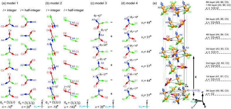
Figure 5: (Color online) Magnetic structure models of PdCrO₂. (a) One solution of a single-$q$ 120^∘ spin structure of the model (1) at 2 K. Here, the solution of the domain given by $\bm{q}_{1}$ and $\bm{q}_{4}$. The magnetic domain of $\bm{q}_{1}=(\frac{1}{3},\frac{1}{3},0)$ gives rise to integer-$l$ reflections of ($\frac{1}{3},\frac{1}{3},l$), while that of $\bm{q}_{4}=(\frac{1}{3},\frac{1}{3},\frac{1}{2}$) provide half-integer-$l$ reflections. 18 arrows labeled by A_n, B_n and C_n ($n=0,1,...5$) represent 18 sublattice spins $S_{\mathrm{A}_{n}}$, $S_{\mathrm{B}_{n}}$ and $S_{\mathrm{C}_{n}}$, respectively. (b) A single-$q$ collinear spin structure of the model (2). Magnetic domains of $\bm{q}_{1}$ and $\bm{q}_{4}$ are shown. Closed circles in the structure of $\bm{q}_{4}$ indicate $S=0$. (c) One of the solutions of the coplanar 120^∘ spin structure of the model (3) at 2 K. Clockwise and anticlockwise rotational directions are represented by $+$ and $-$. The alternative stacks of the $+$ and $-$ layers shown in the figure represent the best fit result, i.e., the $+-+-+-$ structure. (d) One of the solutions of the non-coplanar spin structure of the model (4) at 2 K. The non-coplanarity of spins arises from a rotation of the 120^∘ spin plane around the $c$ axis in subsequent $z$-layers, that is, the azimuthal angles of the normal vector to the 120^∘ spin plane, $\alpha_{n}$ ($n=0,1,2,3,4,5$), are different for each layer. Here a case of which there is only a difference between $\alpha_{n}$ of even layers ($n=0,2,4$) and that of odd layers ($n=1,3,5$) is considered. (e) Schematic drawing of layered triangular network of Cr atoms with spins of the model structure of (d). $\hat{{\bm{a}}}_{\mathrm{M}}$, $\hat{{\bm{b}}}_{\mathrm{M}}$ and $\hat{{\bm{c}}}_{\mathrm{M}}$ represent the magnetic unit cell vectors, consisting of the magnetic structure of the 18 sublattices of Cr ions: $\hat{{\bm{a}}}_{\mathrm{M}}=2\hat{{\bm{a}}}+\hat{{\bm{b}}}$, $\hat{{\bm{b}}}_{\mathrm{M}}=\hat{{\bm{a}}}+2\hat{{\bm{b}}}$, and $\hat{{\bm{c}}}_{\mathrm{M}}=2\hat{{\bm{c}}}$. Here, $\hat{{\bm{a}}}$, $\hat{{\bm{b}}}$, and $\hat{{\bm{c}}}$ are the unit-cell vectors for the hexagonal lattice setting ($\hat{{\bm{a}}}=a\hat{{\bm{x}}}$, $\hat{{\bm{b}}}=a(-\frac{1}{2}\hat{{\bm{x}}}+\frac{\sqrt{3}}{2}\hat{{\bm{y}}})$, $\hat{{\bm{c}}}=c\hat{{\bm{z}}}$, where $\hat{{\bm{x}}}$, $\hat{{\bm{y}}}$, and $\hat{{\bm{z}}}$ are orthogonal unit vectors, and $a$ and $c$ are the lattice constants, respectively).

Least square fits were performed with four parameters for the model (1); $S$ and $\alpha$ for both integer- and half-integer-$l$ domain structures. For the model (2), we used six parameters; $S_{x}$, $S_{y}$, $S_{z}$ for both integer- and half-integer-$l$ domain structures. Here, $S_{x}$, $S_{y}$ and $S_{z}$ are parameters having a relation that $\bm{a}_{j}=\frac{1}{2}S\left(\cos\beta\hat{{\bm{z}}}+\sin\beta\hat{\bm{e}}_{\alpha}\right)e^{i\phi}=(S_{x}\hat{{\bm{x}}}+S_{y}\hat{{\bm{y}}}+S_{z}\hat{{\bm{z}}})e^{i\phi}$. The model (3) considered seven parameters, $S$, $\alpha$, $\phi_{n}$ ($n=1,2,3,4,5$), and examined eight independent classes of magnetic structures. In the analysis, we fixed $\phi_{0}=0^{\circ}$ and considered deviation from it for other angles of $\phi_{n}$. For the model (4), we considered five parameters, $S$, $\phi_{i}$, $\phi_{j}$, $\alpha_{i}$, and $\alpha_{j}$ ($i=0,2,4$, $j=1,3,5$). The fit results are summarized in Tables II, III, IV, and V in the Supplemental Material sup .

Spin structures corresponding to a set of obtained parameters at 2 K are shown in Figs. 5(a)-(d). $\chi^{2}$ values of each result and $R$-factors are summarized in Tables 3 and 4. Here, $\chi^{2}$ is defined by

$$\chi^{2}=\sum_{i=1}^{m}\biggr{(}\frac{|F_{\mathrm{M}}|^{2}_{\mathrm{obs},i}-|F_{\mathrm{M}}|^{2}_{\mathrm{cal},i}}{\sigma(|F_{\mathrm{M}}|^{2}_{\mathrm{obs},i})}\biggl{)}^{2},$$ (17)

where $m=58$ is the number of the observed magnetic reflections. A good fit requires $S^{\prime}=[\chi^{2}/(m-\delta)]^{\frac{1}{2}}\lessapprox 1.3$ where the number of fit parameters $\delta$ is subtracted from the number of reflections $m$. For the model (1), we found $S^{\prime}(2\mathrm{K})=6.6$ and $S^{\prime}(30\mathrm{K})=5.7$. Fits with the model (1) and spins in the $ab$ plane did not improve the value of $S^{\prime}$; $S^{\prime}(2~{}\mathrm{K})=8.2$ and $S^{\prime}(30~{}\mathrm{K})=7.3$. For the model (2), we found good fit results, $S^{\prime}(2\mathrm{K})=1.0$ and $S^{\prime}(30\mathrm{K})=1.0$, but an unphysically large ordered moment as discussed below (cf. Table 3). Within the model (3), the $+-+-+-$ structure class yields by far the best fit result (Table. 4), with $S^{\prime}(2\mathrm{K})=1.1$ and $S^{\prime}(30\mathrm{K})=1.2$. We obtained several solutions in this structure class with the same values of $S^{\prime}$. When evaluating the explicit mathematical form of Eq. (5), we always find two large near-equal amplitudes, either $|\bm{a}_{1}|$ and $|\bm{a}_{5}|$ for ($\bm{q}_{1},\bm{q}_{5}$) or, equivalently, $|\bm{a}_{2}|$ and $|\bm{a}_{6}|$ for ($\bm{q}_{2},\bm{q}_{6}$), or $|\bm{a}_{3}|$ and $|\bm{a}_{4}|$ for ($\bm{q}_{3},\bm{q}_{4}$) with all other amplitudes being an order of magnitude smaller. This resembles the case of LiCrO₂ which is an analogous magnet with the same arrangement of Cr-sites, and implies a double-$q$ structure Kadowaki et al. (1995). We will discuss this result on the basis of the representation analysis in the later section. For the model (4), an acceptable $S^{\prime}$ value was obtained for a case that $\varDelta\alpha_{n}=\alpha_{n}-\alpha_{n-1}\leq 40^{\circ}$: $S^{\prime}(2\mathrm{K})=1.1$ and $S^{\prime}(30\mathrm{K})=1.1$. Within this model we also obtained several solutions, all of which indicate a finite $\varDelta\alpha_{n}$, leading to a non-coplanar spin configuration. Similar to the case of the model(3), two amplitudes $|\bm{a}_{j}|$ are always large, the other small. The estimated value of the average local scalar spin chirality given in Eq. (24) is almost the same for all solutions, although there are small differences in the value of $\phi_{n}$ and that of $\alpha_{n}$ among the solutions.

The estimated magnetic moments at 2 K are listed in Table 3. The magnetic moment value for the model (2) clearly exceeds the expected value of 3$\mu_{\mathrm{B}}$ for the Cr³⁺ magnetic system Brown et al. (2002); Kadowaki et al. (1990), which is unphysical. We therefore can rule out the model (2). Instead, the values for models (3) and (4) are about 30% smaller than the expectation. For 2D spin systems, the magnetic moment is indeed expected to be smaller than $g\mu_{\mathrm{B}}S$ due to quantum effects Mekata et al. (1993); Kadowaki et al. (1995). Moreover, a reduction of the magnetic moment is known in materials with antiferromagnetic coupling and covalent bonding Brown et al. (2002). It can be attributed to hybridization of orbitals between magnetic and neighboring-ligand ions. Therefore, the result of models (3) and (4) can be considered relevant. We note that the magnetic moment is the same in all the solutions in both models (3) and (4). With these results and the requirement for the $\chi^{2}$ value, at 2 K the structure of the $+-+-+-$ structure of the model (3) or the model (4) are considered to be plausible for the magnetic structure of PdCrO₂. At 30 K, the analysis provided almost the same result as at 2 K, with a slight preference of the model (4) compared to the model (3), cf. Table 4. In Sect. IV, we discuss these magnetic structures in the context of the UAHE.

III.3.6 Representation analysis

Before going to the discussion paragraph of Sect. IV, we here discuss symmetry properties of the magnetic structures from the representation analyses. We focus on the analysis using model magnetic structures deduced from the irreducible representation of the crystal symmetry, and then discuss symmetries of models (3) and (4). Characterizations of other models (1) and (2) and details of the symmetry argument are summarized in the appendix.

From fit results of models (3) and (4) discussed in the former section (Sect. III.3.5), let us consider a double-$q$ structure such that consists of ($\bm{q}_{1},\bm{q}_{5}$), ($\bm{q}_{2},\bm{q}_{6}$), or ($\bm{q}_{3},\bm{q}_{4}$). In view of the representation analysis, these combinations are the simplest combinations that can lead to a magnetic structure having a 120^∘-spin plane, since the basis vectors of such two wave vectors consist of similar components (Table 8). The double-$q$ structure is written as, for example,

$$\bm{S}(\bm{R})=\sum_{j=3}^{4}\left\{\bm{b}_{j}\exp(i\bm{q}_{j}\cdot\bm{R})+\bm{b}_{j}^{*}\exp(-i\bm{q}_{j}\cdot\bm{R})\right\},$$ (18)

$$\bm{b}_{3}=C_{3\Gamma_{1}1}\bm{\psi}_{3\Gamma_{1}1}+C_{3\Gamma_{2}1}\bm{\psi}_{3\Gamma_{2}1},+C_{3\Gamma_{2}2}\bm{\psi}_{3\Gamma_{2}2},$$ (19)

$$\bm{b}_{4}=C_{4\Gamma_{1}1}\bm{\psi}_{4\Gamma_{1}1}+C_{4\Gamma_{1}2}\bm{\psi}_{4\Gamma_{1}2},+C_{4\Gamma_{2}1}\bm{\psi}_{4\Gamma_{2}1},$$ (20)

where $\bm{R}=\bm{t}_{n}+\bm{d}$, $\bm{t}_{n}$ and $\bm{d}$ are the $n$-th lattice position and a coordinate of the magnetic site of the chromium atoms (i.e., $\bm{d}=(0,0,\frac{1}{2})$, the 3b site of $R\bar{3}m$), respectively, $C_{j\Gamma_{k}l}$ is a complex coefficient, and $\bm{\psi}_{j\Gamma_{k}l}$ is a basis vector of the irreducible representation for the space group $R\bar{3}m$ appearing in the $l$-th basis of a small representation $\Gamma_{k}$ with $\bm{q}_{j}$ (Table 8).

Least square fits were performed with six parameters of $C_{j\Gamma_{k}l}$ and show an excellent fit result with $\chi^{2}=50$. The parameters for results at 2 K were obtained as

$$C_{3\Gamma_{1}1}=(0\pm 16){\rm{e}}^{i\phi_{3\Gamma_{1}1}},$$

$$C_{3\Gamma_{2}1}=(0.15\pm 0.01){\rm{e}}^{i\phi_{3\Gamma_{2}1}},$$

$$C_{3\Gamma_{2}2}=(0.54\pm 0.01){\rm{e}}^{i\phi_{3\Gamma_{2}2}},$$

$$C_{4\Gamma_{1}1}=-(0.52\pm 0.01){\rm{e}}^{i\phi_{4\Gamma_{1}1}},$$

$$C_{4\Gamma_{1}2}=(0.16\pm 0.01){\rm{e}}^{i\phi_{4\Gamma_{1}2}},$$

$$C_{4\Gamma_{2}1}=(0.08\pm 0.03){\rm{e}}^{i\phi_{4\Gamma_{2}1}}.$$

Note that since multiplication of a phase factor ${\rm{e}}^{i\phi_{j\Gamma_{k}l}}$ doesn’t change the scattering intensity, $\phi_{j\Gamma_{k}l}$ is a certain constant. We confirmed that obtained parameters of $C_{j\Gamma_{k}l}$ appear to be consistent with the parameters of the fitted structure of the model (4), leading to a non-coplanar 120^∘-spin structure. In fact, the structure shown in Fig. 5(d) is reproduced by Eq. (18) with $C_{3\Gamma_{1}1}=-(0.06\pm 0.01){\rm{e}}^{i\phi_{3\Gamma_{1}1}}$, $C_{3\Gamma_{2}1}=(0.15\pm 0.01){\rm{e}}^{i\phi_{3\Gamma_{2}1}}$, $C_{3\Gamma_{2}2}=(0.53\pm 0.01){\rm{e}}^{i\phi_{3\Gamma_{2}2}}$, $C_{4\Gamma_{1}1}=-(0.52\pm 0.01){\rm{e}}^{i\phi_{4\Gamma_{1}1}}$, $C_{4\Gamma_{1}2}=(0.16\pm 0.01){\rm{e}}^{i\phi_{4\Gamma_{1}2}}$, and $C_{4\Gamma_{2}1}=(0.07\pm 0.01){\rm{e}}^{i\phi_{4\Gamma_{2}1}}$, where $\phi_{3\Gamma_{1}1}=72^{\circ}\pm 2^{\circ}$, $\phi_{3\Gamma_{2}1}=-2^{\circ}\pm 2^{\circ}$, $\phi_{3\Gamma_{2}2}=1^{\circ}\pm 1^{\circ}$, $\phi_{4\Gamma_{1}1}=1^{\circ}\pm 0.3^{\circ}$, $\phi_{4\Gamma_{1}2}=1^{\circ}\pm 4^{\circ}$, and $\phi_{4\Gamma_{2}1}=-14^{\circ}\pm 2^{\circ}$, respectively. Thus, we can now recognize that the model (4) structure is a double-$q$ structure consisting of all the small representations of two wave vectors. Note that although $\phi_{j\Gamma_{k}l}$ is difficult to be determined only from the analysis of the scattering intensity by Eqs. (18)–(20), we can deduce such parameter from the fitted structure of the model (4) and its representation analysis, as shown above. More detailed experiments are needed to clarify precise values of $\phi_{j\Gamma_{k}l}$.

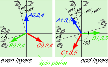
Figure 6: (Color online) Relations of the spin configurations of the model (3) structure for each layer, deduced from the representation analysis. The rotational direction of the spins on even and odd layers is opposite, i.e., the $+-+-+-$ structure is realized. Definitions of $\hat{\bm{e}}_{1}$ and $\hat{\bm{e}}_{2}$ axes are in the text. Here, $\phi^{\prime}=16^{\circ}$ and $\phi^{\prime\prime}=-16^{\circ}$, respectively. The $\hat{\bm{c}}$ axis is parallel to the $\bm{z}$ axis and $\hat{\bm{e}}_{30^{\circ}}$ is the direction of the spin plane; $\hat{\bm{e}}_{30^{\circ}}=\frac{\sqrt{3}}{2}\hat{{\bm{x}}}+\frac{1}{2}\hat{{\bm{y}}}$ (see text for more details).

It is worth noting here that even though we assumed that smaller contributions of $\bm{\psi}_{3\Gamma_{1}1}$ and $\bm{\psi}_{4\Gamma_{2}1}$ were negligible and those coefficients were zero for the analysis by Eqs. (18)–(20), we also reproduced the scattering intensities with good fittings ($\chi^{2}=51$). This structure is a coplanar structure, corresponding to the $+-+-+-$ structure of the model (3). From the fittings, we confirmed that the magnetic structure shown in Fig. 5(c) is approximately represented by using parameters with $C_{3\Gamma_{2}1}\simeq\frac{S}{2}\sin(\phi^{\prime}){\rm e}^{i\phi^{\prime\prime}}$, $C_{3\Gamma_{2}2}\simeq\frac{S}{2}\cos(\phi^{\prime}){\rm e}^{i\phi^{\prime\prime}}$, $C_{4\Gamma_{1}1}\simeq-\frac{S}{2}\cos(\phi^{\prime}){\rm e}^{i\phi^{\prime\prime}}$, and $C_{4\Gamma_{1}2}\simeq\frac{S}{2}\sin(\phi^{\prime}){\rm e}^{i\phi^{\prime\prime}}$, where $S=1.09\pm 0.06$, $\phi^{\prime}=16^{\circ}\pm 1^{\circ}$ and $\phi^{\prime\prime}=-16^{\circ}\pm 1^{\circ}$, respectively. Thus, it is clear that the $+-+-+-$ structure of the model (3) is also a double-$q$ structure, written by the linear combination of two of three small representations for each wave vector of e.g. ($\bm{q}_{3},\bm{q}_{4}$). In this case, Eq. (18) is summarized as follows:

$$\bm{S}(\bm{R})=\frac{S}{2}\cos\Bigl{(}\bm{q}_{3}\cdot\bm{R}-\phi^{\prime\prime}\Bigr{)}\hat{\bm{e}}_{1}$$

$$\hskip 60.0pt+\frac{S}{2}\sin\Bigl{(}\bm{q}_{4}\cdot\bm{R}-\frac{\pi}{2}-\phi^{\prime\prime}\Bigr{)}\hat{\bm{e}}_{2}$$ (21)

$$\hat{\bm{e}}_{1}=\cos\Bigl{(}\phi^{\prime}\Bigr{)}\hat{\bm{z}}+\sin\Bigl{(}\phi^{\prime}\Bigr{)}\hat{\bm{e}}_{30^{\circ}}$$ (22)

$$\hat{\bm{e}}_{2}=\cos\Bigl{(}\phi^{\prime}+\frac{\pi}{2}\Bigr{)}\hat{\bm{z}}+\sin\Bigl{(}\phi^{\prime}+\frac{\pi}{2}\Bigr{)}\hat{\bm{e}}_{30^{\circ}}.$$ (23)

Calculated values of $\bm{q}_{3}\cdot\bm{R}$ and $\bm{q}_{4}\cdot\bm{R}-\pi/2$ are shown in Table 5. Since values of $\bm{q}_{4}\cdot\bm{R}-\pi/2$ are different in $\pi(=180^{\circ})$ for even and odd layers, the rotation direction of the spin plane becomes opposite for those layers. This is the reason why the $+-+-+-$ structure is realized in the model (3). Details of the spin configurations and relations between vectors of $\hat{\bm{e}}_{1}$ and $\hat{\bm{e}}_{2}$ are shown in Fig. 6. Other results for the representation analysis of models (1) and (2) are summarized in the appendix.

Table 5: Calculated values of $\bm{q}_{3}\cdot\bm{R}$ and $\bm{q}_{4}\cdot\bm{R}-\pi/2$ for each sublattice site. $i=0,2,4$ and $j=1,3,5$ indicate suffixes of the sublattice sites of even and odd layers, respectively.

$\bm{R}$	$\bm{q}_{3}\cdot\bm{R}$	$\bm{q}_{4}\cdot\bm{R}-\pi/2$
$(i=0,2,4)$
$\bm{R}_{\text{A}_{i}}$	0	0
$\bm{R}_{\text{B}_{i}}$	$2\pi/3$	$2\pi/3$
$\bm{R}_{\text{C}_{i}}$	$4\pi/3$	$4\pi/3$
$(j=1,3,5)$
$\bm{R}_{\text{A}_{j}}$	0	$\pi$
$\bm{R}_{\text{B}_{j}}$	$2\pi/3$	$2\pi/3+\pi$
$\bm{R}_{\text{C}_{j}}$	$4\pi/3$	$4\pi/3+\pi$

IV Discussion

For rhombohedral antiferromagnet with the delafossite type structure, the magnetic state is expected to display a helical structure and to be highly degenerate Rastelli and Tassi (1986, 1988); Reimers and Dahan (1992). The structure may become incommensurate due to certain competition among the nearest-neighbor and longer-range exchange interactions. Experimentally, it was found recently that the magnetic structures of CuCrO₂ and AgCrO₂, which belong to the same magnetic Cr delafossite family as PdCrO₂, are incommensurate with a propagation vector $q=(kk0)$ [$k\sim 0.329$ for CuCrO₂ and $0.327$ for AgCrO₂]. Their magnetic structures are considered to be proper-screw type structures with {110} spiral planes Poienar et al. (2009); Soda et al. (2009); Oohara et al. (1994). In contrast, we found that a commensurate magnetic structure is realized in PdCrO₂. The transition temperature as a function of the lattice parameter $a$ reveals a linear relation in the delafossites $A$CrO₂ ($A=\mathrm{Pd},\mathrm{Cu},\mathrm{Ag}$) and the ordered-rock salts $A^{\prime}$CrO₂ ($A^{\prime}=\mathrm{Li},\mathrm{Na},\mathrm{K}$), which all have a similar TL arrangement of Cr ions [Fig. 7(a)]. Meanwhile, the $c$-axis length does not exhibit a simple relation with the value of $T_{\mathrm{N}}$ [Fig. 7(b)]. Interestingly, systems that have smaller $a$ values (i.e., LiCrO₂ and PdCrO₂) exhibit commensurate magnetic structures with magnetic Bragg reflections of ($\frac{1}{3}$ $\frac{1}{3}$ $l$) with $l=$ integers and half integers (i.e., a commensurate double-$q$ structure), while systems that have larger $a$ values exhibit peculiar magnetic order including incommensurate magnetic orders Poienar et al. (2009); Soda et al. (2009); Oohara et al. (1994); Olariu et al. (2006). These results suggest that, while the nearest neighbor exchange interaction is predominant in all these materials, types of other interactions are quite different between materials with smaller $a$ and those with larger $a$.

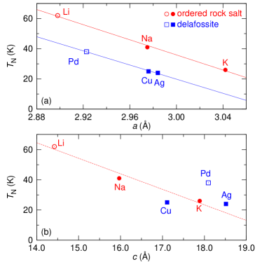
Figure 7: (Color online) Relation between $T_{\mathrm{N}}$ and lattice parameters $a$ and $c$ of chromium ordered-rock salts and delafossites $A$CrO₂ (ordered rock salts: $A=\mathrm{Li},\mathrm{Na},\mathrm{K}$, delafossites: $A=\mathrm{Pd},\mathrm{Cu},\mathrm{Ag}$). The horizontal axis displays the lattice parameters at RT Delmas et al. (1978); Soubeyroux et al. (1979); Shannon et al. (1971); Angelov and Doumerc (1991). Open and filled symbols represent materials that have commensurate magnetic structures and ones that have incommensurate magnetic structures, respectively. In materials with smaller lattice constant $a$, a commensurate magnetic structure is realized probably because the nearest-neighbor interaction $J$ is much larger than other interactions.

Our analysis of the magnetic structure leaves us with two possibilities for the magnetic structure of PdCrO₂, the $+-+-+-$ 120^∘ spin structures of the model (3) and the model (4). The difference in the magnetic intensity between these models is too small to distinguish them (Fig. 4). However, the coplanar $+-+-+-$ spin structure of the model (3) has no scalar spin chirality and hence cannot produce an anomalous Hall current by the mechanism of the scalar spin chirality. Even in an applied magnetic field along the $c$ axis, the scalar spin chirality is zero because the induced spin canting would be parallel to the $c$ axis and hence still within the 120^∘ spin plane. In contrast, the model (4) structure has a non-coplanar spin configuration with a locally-finite scalar spin chirality. Note that the mechanism of UAHE on the basis of the Berry-phase concept with the four-site magnetic structure Shindou and Nagaosa (2001); Martin and Batista (2008); Akagi and Motome (2010) could be excluded for the case of PdCoO₂, because magnetic Bragg peaks are observed at $(\frac{1}{3},\frac{1}{3},l)$ and $(\frac{2}{3},\frac{2}{3},l)$, consisting of the three sublattice magnetic structure. We will argue now that within the model (4) structure the spin chirality mechanism could generate an UAHE. First we note that the global sum of the scalar spin chiralities is zero in the model (4) structure. This result implies that an additional contribution is needed to break the balance of the globally zero scalar spin chirality. One possible mechanism is in the spin-orbit interaction Tatara and Kawamura (2002); Kawamura (2003). The spin-orbit interaction breaks the perfect cancellation of local scalar spin chiralities in the presence of a net magnetization induced by an magnetic field. This gives then rise to an fine contribution to the UAHE Tatara and Kawamura (2002); Kawamura (2003).

From the representation analysis, the non-coplanar magnetic structure can be deduced from the symmetry properties of the $R\bar{3}m$ crystal structure of PdCrO₂. In particular, the model (4) structure is characterized by additional appearance of small representations such as $\Gamma_{1}1$ of $\bm{q}_{3}$ and $\Gamma_{2}1$ of $\bm{q}_{4}$. In view of the free-energy expansion, a higher-order term, 3rd or 4th, involving those small representations becomes important for the realization of the non-coplanar double-$q$ structure, since the simple Heisenberg type interaction with a small finite single-ion anisotropy as given by Eq. (1), the model (1) simplest-120^∘-spin structure (i.e., single-$q$ coplanar-120^∘-spin structure) should be realized. More quantitative analysis is required to explain why the structure appears in PdCrO₂.

Finally, we discuss the small change of the magnetic structure between 2 K and 30 K. Since the UAHE occurs in this material below $T^{*}$, we can consider two scenarios: One is the change from the coplanar to non-coplanar spin structures at temperatures between 2 and 30 K. The other scenario is the change of the amount of the non-coplanarity with temperature: i.e., a non-coplanar spin structure is already realized at 30 K and the amount of non-coplanarity (or local scalar spin chirality) changes on cooling. To evaluate the non-coplanarity in the magnetic structure, we calculate the average absolute value of the local scalar spin chirality over the 18 sublattice spins,

$$v=\frac{\displaystyle\sum_{i,j,k}^{18}\Bigr{|}\bm{S}_{i}\cdot(\bm{S}_{j}\times\bm{S}_{k})\Bigl{|}}{|M|^{3}},$$ (24)

where $M$ is the magnetic moment of each Cr spin, and $\bm{S}_{i}$ represents a spin component such as $\bm{S}_{1}=\bm{S}_{\mathrm{A}0}$, $\bm{S}_{2}=\bm{S}_{\mathrm{B}0}$, $\bm{S}_{3}=\bm{S}_{\mathrm{C}0}$, and etc. ($i\neq j\neq k$). In Eq. (24), we normalize the absolute local scalar spin chirality by $M^{3}$ in order to estimate the amount of non-coplanarity independent of the length of the ordered moment. Although a weight of a spin-chirality contribution depends on a size of a triangle formed by three non-coplanar spinsTatara and Kawamura (2002), we calculate a simple sum of $\bm{S}_{i}\cdot(\bm{S}_{j}\times\bm{S}_{k})$ in 18 magnetic sublattices, without considering each the weight of each for the UAHE. From the fit results of the model (4), we obtained $v(2~{}\mathrm{K})=0.010(4)$ and $v(30~{}\mathrm{K})=0.026(4)$. This result suggests that a slight difference appears in the non-coplanarity of the magnetic structures between 2 K and 30 K. However, the value at 30 K is a bit larger than that at 2 K. Even if the sum of chiralities given Eq. (24) was not normalized by $M^{3}$, the value at 2 K is smaller. If the second scenario is correct, the weight of $\bm{S}_{i}\cdot(\bm{S}_{j}\times\bm{S}_{k})$ from each triangle for the UAHE is different, depending on the size of triangles or carrier mobility $\mu$: a larger carrier mobility makes the conduction carriers interact with a larger number of spins of the non-coplanar structure Tatara and Kawamura (2002). This result leads to the change in the anomalous Hall conductivity $\sigma_{xy}$ originating in the scalar spin chirality $\chi_{ijk}$, if $\chi_{ijk}$ is finite, because $\sigma_{xy}$ is closely related to both $\mu$ and $\chi_{ijk}$: $\sigma_{xy}\propto\mu^{2}\chi_{ijk}$ [Ref. Tatara and Kawamura, 2002]. Experimentally, it was estimated that the mean free path at 2 K is about ten times larger than that at 30 K Takatsu and Maeno (2010). Otherwise, the first scenario may be more likely to explain the occurrence of the UAHE. In any case, a precise estimation of the knowledge of the weight of $\bm{S}_{i}\cdot(\bm{S}_{j}\times\bm{S}_{k})$ of each triangle is important, and here the trajectory of conduction carriers should be taken into account. The multiple-$q$ state of the magnetic structure may also be important Okubo et al. (2012). We now conclude that the difference of the magnetic structure between 2 K and 30 K is small but may result from the non-coplanarity (misfit of stacks for 120^∘ layers) of the magnetic structure. Such a minute change of the magnetic structure is consistent with a small change of the intensity ratio of magnetic reflections (Fig. 2 inset) and of entropy associated with a small hump in the magnetic specific heat at $T^{*}$ [Ref. Takatsu et al., 2009].

V Conclusions

In conclusion, we performed neutron single crystal and X-ray powder diffraction experiments on the metallic 2D-TL antiferromagnet PdCrO₂ in zero field. We found that at 2 K the magnetic structure of Cr spins is a commensurate 120^∘-spin structure where the spin plane includes the $c$ axis. It alternates clockwise and anticlockwise rotation in different Cr layers. Non-coplanar spin configurations, with an additional rotation of the spin plane agree with the data slightly better than the coplanar model. In view of the observed UAHE, such a non-coplanar 120^∘-spin structure is probably realized in PdCrO₂, which is a double-$q$ structure derived by the representation analysis. The identification of a precise non-coplanarity as well as the magnetic structure in an applied magnetic field should be addressed by future experiments on much larger single crystals using polarized neutrons.

Appendix

Table 6: Coordinate triple of the representative symmetry operator $\{\gamma|\tau_{\gamma}\}$.

	$\bm{q}_{1}$, $\bm{q}_{5}$	$\bm{q}_{2}$, $\bm{q}_{6}$	$\bm{q}_{3}$, $\bm{q}_{4}$
$\{\gamma|\tau_{\gamma}\}_{1}$	$(x,y,z)$	$(x,y,z)$	$(x,y,z)$
$\{\gamma|\tau_{\gamma}\}_{2}$	$(y,x,-z)$	$(x-y,-y,-z)$	$(-x,-x+y,-z)$

Table 7: Matrix $D_{k}(\{\gamma|\tau_{\gamma}\})$ of Eq.(25) for small representations $\Gamma_{k}$.

rep.	$\{\gamma|\tau_{\gamma}\}_{1}$	$\{\gamma|\tau_{\gamma}\}_{2}$
$\Gamma_{1}$	1	1
$\Gamma_{2}$	1	-1

Table 8: The basis vectors $\bm{\psi}_{j\Gamma_{k}l}$ of the irreducible representations of the space group $R\bar{3}m$ (point group $D^{5}_{3d}$) appearing in the $l$-th basis of a small representation $\Gamma_{k}$ with $\bm{q}_{j}$. The notation of vectors $\hat{{\bm{e}}}_{\alpha}$ used here is defined in the main text and the relations with other directions are schematically shown in Figs. 5 and 8.

$\bm{q}_{j}\,(j=1-6)$	$\bm{q}_{1}$	$\bm{q}_{2}$	$\bm{q}_{3}$	$\bm{q}_{4}$	$\bm{q}_{5}$	$\bm{q}_{6}$
$\bm{\psi}_{j\Gamma_{1}1}$	$\hat{{\bm{e}}}_{60^{\circ}}$	$\hat{{\bm{e}}}_{0^{\circ}}$	$\hat{{\bm{e}}}_{-60^{\circ}}$	$\hat{{\bm{e}}}_{30^{\circ}}$	$\hat{{\bm{e}}}_{150^{\circ}}$	$\hat{{\bm{e}}}_{90^{\circ}}$
$\bm{\psi}_{j\Gamma_{1}2}$				$\hat{{\bm{z}}}$	$\hat{{\bm{z}}}$	$\hat{{\bm{z}}}$
$\bm{\psi}_{j\Gamma_{2}1}$	$\hat{{\bm{e}}}_{150^{\circ}}$	$\hat{{\bm{e}}}_{90^{\circ}}$	$\hat{{\bm{e}}}_{30^{\circ}}$	$\hat{{\bm{e}}}_{-60^{\circ}}$	$\hat{{\bm{e}}}_{60^{\circ}}$	$\hat{{\bm{e}}}_{0^{\circ}}$
$\bm{\psi}_{j\Gamma_{2}2}$	$\hat{{\bm{z}}}$	$\hat{{\bm{z}}}$	$\hat{{\bm{z}}}$

Table 9: Relations between the model magnetic structures and the results of the representation analysis.

model	type	example	rep.	basis vector
model (1)	single-$q$,	$\bm{q}_{1}$ domain (integer $l$)	$\Gamma_{2}1$, $\Gamma_{2}2$	$\bm{\psi}_{1\Gamma_{2}1}$, $\bm{\psi}_{1\Gamma_{2}2}$
	multiple domain	$\bm{q}_{4}$ domain (half-int. $l$)	$\Gamma_{1}1$, $\Gamma_{1}2$	$\bm{\psi}_{4\Gamma_{1}1}$, $\bm{\psi}_{4\Gamma_{1}2}$
model (2)	single-$q$,	$\bm{q}_{1}$ domain (integer $l$)	$\Gamma_{2}1$, $\Gamma_{2}2$	$\bm{\psi}_{1\Gamma_{2}1}$, $\bm{\psi}_{1\Gamma_{2}2}$
	multiple domain	$\bm{q}_{4}$ domain (half-int. $l$)	$\Gamma_{1}1$, $\Gamma_{1}2$	$\bm{\psi}_{4\Gamma_{1}1}$, $\bm{\psi}_{4\Gamma_{1}2}$
model (3)	double-$q$,	($\bm{q}_{3}$,$\bm{q}_{4}$) domain	$\Gamma_{2}1$, $\Gamma_{2}2$	$\bm{\psi}_{3\Gamma_{2}1}$, $\bm{\psi}_{3\Gamma_{2}2}$
	multiple domain		$\Gamma_{1}1$, $\Gamma_{1}2$	$\bm{\psi}_{4\Gamma_{1}1}$, $\bm{\psi}_{4\Gamma_{1}2}$
model (4)	double-$q$,	($\bm{q}_{3}$,$\bm{q}_{4}$) domain	$\Gamma_{1}1$, $\Gamma_{2}1$, $\Gamma_{2}2$	$\bm{\psi}_{3\Gamma_{1}1}$, $\bm{\psi}_{3\Gamma_{2}1}$, $\bm{\psi}_{3\Gamma_{2}2}$
	multiple domain		$\Gamma_{1}1$, $\Gamma_{1}2$, $\Gamma_{2}1$	$\bm{\psi}_{4\Gamma_{1}1}$, $\bm{\psi}_{4\Gamma_{1}2}$, $\bm{\psi}_{4\Gamma_{2}1}$

Figure 8: (Color online) Schematic drawing of one of the relations of two wave vectors and the spin plane of the model (3) structure. For $\bm{q}_{3}$ and $\bm{q}_{4}$, the spin plane consists of $\hat{\bm{c}}(\parallel\hat{\bm{z}})$ and $\hat{\bm{e}}_{30^{\circ}}(=\frac{\sqrt{3}}{2}\hat{{\bm{x}}}+\frac{1}{2}\hat{{\bm{y}}})$.

In this section, we summarize results of the representation analysis and classification of model magnetic structures using symmetry properties of the space group of $R\bar{3}m$, discussed in Sect. III.3.

The basis vectors $\bm{\psi}_{j\Gamma_{k}l}$ are calculated by using the projection operator method Izyumov et al. (1991). For the little group $G_{\bm{q}_{j}}$ for each wave vector $\bm{q}_{j}$, there are two one-dimensional small representations

$$\Gamma_{k}(\{\gamma|\tau_{\gamma}\})=\exp(-i\bm{q}_{j}\cdot\tau_{\alpha})D_{k}(\{\gamma|\tau_{\gamma}\}),$$ (25)

where $\{\gamma|\tau_{\gamma}\}$ denotes a symmetry operator of $G_{\bm{q}_{j}}$ and $D_{k}(\{\gamma|\tau_{\gamma}\})$ is the matrix of the small representation of $G_{\bm{q}_{j}}$. In Tables 6 and 7, $D_{k}(\{\gamma|\tau_{\gamma}\})$ for each $\bm{q}_{j}$ are summarized. The basis vectors $\bm{\psi}_{j\Gamma_{k}l}$ are calculated by using these matrices and the results are listed in Table 8.

For the single-$q$ structures of models (1) and (2), the magnetic representation of Eqs. (7), (9), (11), and (13) can be re-written by irreducible representations: i.e., Eqs. (7) and (11) for integer-$l$ reflections are

$$\bm{S}(\bm{R})=\bm{b}_{1}\exp(i\bm{q}_{1}\cdot\bm{R})+\bm{b}_{1}^{*}\exp(-i\bm{q}_{1}\cdot\bm{R}),$$ (26)

$$\bm{b}_{1}=C_{1\Gamma_{1}1}\bm{\psi}_{1\Gamma_{1}1}+C_{1\Gamma_{2}1}\bm{\psi}_{1\Gamma_{2}1},+C_{1\Gamma_{2}2}\bm{\psi}_{1\Gamma_{2}2},$$ (27)

and Eqs. (9) and (13) for half-integer-$l$ reflections are

$$\bm{S}(\bm{R})=\bm{b}_{4}\exp(i\bm{q}_{4}\cdot\bm{R})+\bm{b}_{4}^{*}\exp(-i\bm{q}_{4}\cdot\bm{R}),$$ (28)

$$\bm{b}_{4}=C_{4\Gamma_{1}1}\bm{\psi}_{4\Gamma_{1}1}+C_{4\Gamma_{1}2}\bm{\psi}_{4\Gamma_{1}2},+C_{4\Gamma_{2}1}\bm{\psi}_{4\Gamma_{2}1}.$$ (29)

Here, $C_{1\Gamma_{2}1}=C_{4\Gamma_{1}1}=\frac{S}{2}\exp({-\frac{\pi}{2}i})$, $C_{1\Gamma_{2}2}=C_{4\Gamma_{1}2}=\frac{S}{2}$, and $C_{1\Gamma_{1}l}=C_{4\Gamma_{2}l}=0$ for the model (1), and $C_{1\Gamma_{2}1}=C_{4\Gamma_{1}1}=\frac{S}{2}\sin(\beta)$, $C_{1\Gamma_{2}2}=C_{4\Gamma_{1}2}=\frac{S}{2}\cos(\beta)$, and $C_{1\Gamma_{1}l}=C_{4\Gamma_{2}l}=0$ for the model (2), respectively. Note that more generally, the magnetic moment can be represented by summing the results of six-$q$ wave vectors:

$$\bm{S}(\bm{R})=\sum_{j=1}^{6}\left\{\bm{b}_{j}\exp(i\bm{q}_{j}\cdot\bm{R})+\bm{b}_{j}^{*}\exp(-i\bm{q}_{j}\cdot\bm{R})\right\},$$ (30)

$$\bm{b}_{X}=C_{X\Gamma_{1}1}\bm{\psi}_{X\Gamma_{1}1}+C_{X\Gamma_{2}1}\bm{\psi}_{Y\Gamma_{2}1},+C_{X\Gamma_{2}2}\bm{\psi}_{X\Gamma_{2}2},$$ (31)

$$\bm{b}_{Y}=C_{Y\Gamma_{1}1}\bm{\psi}_{Y\Gamma_{1}1}+C_{Y\Gamma_{1}2}\bm{\psi}_{Y\Gamma_{1}2},+C_{Y\Gamma_{2}1}\bm{\psi}_{Y\Gamma_{2}1},$$ (32)

where $X=1,2,3$ and $Y=4,5,6$, respectively. This expression is equal to that of Eq. (5). The relations of model structures and results of the representation analysis are shown in Table 9.

References

- Nagaosa et al. (2010) N. Nagaosa, J. Sinova, S. Onoda, A. H. MacDonald, and N. P. Ong, Rev. Mod. Phys. 82, 1539 (2010).
- Xiao et al. (2010) D. Xiao, M.-C. Chang, and Q. Niu, Rev. Mod. Phys. 82, 1959 (2010).
- Tokura and Seki (2010) Y. Tokura and S. Seki, Adv. Mater. 22, 1554 (2010).
- Arima (2011) T. Arima, J. Phys. Soc. Jpn. 80, 052001 (2011).
- Taguchi et al. (2001) Y. Taguchi, Y. Oohara, H. Yoshizawa, N. Nagaosa, and Y. Tokura, Science 291, 2573 (2001).
- Yasui et al. (2006) Y. Yasui, T. Kageyama, T. Moyoshi, M. Soda, M. Sato, and K. Kakurai, J. Phys. Soc. Jpn. 75, 084711 (2006).
- Machida et al. (2007) Y. Machida, S. Nakatsuji, Y. Maeno, T. Tayama, T. Sakakibara, and S. Onoda, Phys. Rev. Lett. 98, 057203 (2007).
- Machida et al. (2009) Y. Machida, S. Nakatsuji, S. Onoda, T. Tayama, and T. Sakakibara, Nature 463, 210 (2009).
- Matl et al. (1998) P. Matl, N. P. Ong, Y. F. Yan, Y. Q. Li, D. Studebaker, T. Baum, and G. Doubinina, Phys. Rev. B 57, 10248 (1998).
- Ye et al. (1999) J. Ye, Y. B. Kim, A. J. Millis, B. I. Shraiman, P. Majumdar, and Z. Tasanovic, Phys. Rev. Lett. 83, 3737 (1999).
- Ohgushi et al. (2000) K. Ohgushi, S. Murakami, and N. Nagaosa, Phys. Rev. B 62, 6065 (2000).
- Tatara and Kawamura (2002) G. Tatara and H. Kawamura, J. Phys. Soc. Jpn 71, 2613 (2002).
- Tomizawa and Kontani (2009) T. Tomizawa and H. Kontani, Phys. Rev. B 80, 100401 (2009).
- Taguchi and Tatara (2009) K. Taguchi and G. Tatara, Phys. Rev. B 79, 054423 (2009).
- Aharonov and Bohm (1959) Y. Aharonov and D. Bohm, Phys. Rev. 115, 485 (1959).
- Takatsu et al. (2010) H. Takatsu, S. Yonezawa, S. Fujimoto, and Y. Maeno, Phys. Rev. Lett. 105, 137201 (2010).
- Shiomi et al. (2012) Y. Shiomi, M. Mochizuki, Y. Kaneko, and Y. Tokura, Phys. Rev. Lett. 108, 056601 (2012).
- Kawamura (2003) H. Kawamura, Phys. Rev. Lett. 90, 047202 (2003).
- Shindou and Nagaosa (2001) R. Shindou and N. Nagaosa, Phys. Rev. Lett. 87, 116801 (2001).
- Martin and Batista (2008) I. Martin and C. D. Batista, Phys. Rev. Lett. 101, 156402 (2008).
- Akagi and Motome (2010) Y. Akagi and Y. Motome, J. Phys. Soc. Jpn. 79, 083711 (2010).
- Ok et al. (2013) J. M. Ok, Y. J. Jo, K. Kim, T. Shishidou, E. S. Choi, H.-J. Noh, T. Oguchi, B. I. Min, and J. S. Kim, Phys. Rev. Lett. 111, 176405 (2013).
- Sobota et al. (2013) J. A. Sobota, K. Kim, H. Takatsu, M. Hashimoto, S. K. Mo, Z. Hussain, T. Oguchi, T. Shishidou, Y. Maeno, B. I. Min, et al., Phys. Rev. B 88, 125109 (2013).
- Ong and Singh (2012) K. P. Ong and D. J. Singh, Phys. Rev. B 85, 134403 (2012).
- Doumerc et al. (1986) J. P. Doumerc, A. Wichainchai, A. Ammar, M. Pouchard, and P. Hagenmuller, Mat. Res. Bull. 21, 745 (1986).
- Mekata et al. (1995) M. Mekata, T. Sugino, A. Oohara, Y. Oohara, and H. Yoshizawa, Physica B 213, 221 (1995).
- Takatsu et al. (2009) H. Takatsu, H. Yoshizawa, S. Yonezawa, and Y. Maeno, Phys. Rev. B 79, 104424 (2009).
- Hirone and Adachi (1957) T. Hirone and K. Adachi, J. Phys. Soc. Jpn. 12, 156 (1957).
- Hurd (1972) C. M. Hurd, The Hall effect in metals and alloys (Plenum Press, New York, 1972).
- Takatsu and Maeno (2010) H. Takatsu and Y. Maeno, J. Cryst. Growth 312, 3461 (2010).
- Izumi and Momma (2007) F. Izumi and K. Momma, Solid State Phenom. 130, 15 (2007).
- (32) H. Takatsu et. al., unpublished.
- Fujiki et al. (1983) S. Fujiki, K. Shutoh, yoshihiko Abe, and S. Katsura, J. Phys. Soc. Jpn. 52, 1531 (1983).
- Blankschtein et al. (1984) D. Blankschtein, M. Ma, and A. N. Berker, Phys. Rev. B 29, 5250 (1984).
- Kimura et al. (2008) K. Kimura, H. Nakamura, K. Ohgushi, and T. Kimura, Phys. Rev. B 78, 140401(R) (2008).
- (36) Supplemental Material for the observed and calculated structure factors.
- Hemmeida et al. (2011) M. Hemmeida, H.-A. K. von Nidda, and A. Loidl, J. Phys. Soc. Jpn. 80, 053707 (2011).
- Kadowaki et al. (1995) H. Kadowaki, H. Takei, and K. Motoya, J. Phys. Cond. Matt. 7, 6869 (1995).
- Brown et al. (2002) P. J. Brown, J. B. Forsyth, and F. Tasset, J. Phys.: Cond. Matt. 14, 1957 (2002).
- Kadowaki et al. (1990) H. Kadowaki, H. Kikuchi, and Y. Ajiro, J. Phys. Cond. Matt. 2, 4485 (1990).
- Mekata et al. (1993) M. Mekata, N. Yaguchi, T. Takagi, T. Sugino, S. Mituda, H. Yoshizawa, N. Hosoito, and T. Shinjo, J. Phys. Soc. Jpn. 62, 4474 (1993).
- Rastelli and Tassi (1986) E. Rastelli and A. Tassi, J. Phys. C: Solid State Phys. 19, L423 (1986).
- Rastelli and Tassi (1988) E. Rastelli and A. Tassi, J. Phys. C: Solid State Phys. 21, 1003 (1988).
- Reimers and Dahan (1992) J. N. Reimers and J. R. Dahan, J. Phys. Cond. Matt. 4, 8105 (1992).
- Poienar et al. (2009) M. Poienar, F. Damay, C. Martin, V. Hardy, A. Maignan, and G. Andre, Phys. Rev. B 79, 014412 (2009).
- Soda et al. (2009) M. Soda, K. Kimura, T. Kimura, M. Matsuura, and K. Hirota, J. Phys. Soc. Jpn. 78, 124703 (2009).
- Oohara et al. (1994) Y. Oohara, S. Mitsuda, H. Yoshizawa, N. Yaguchi, H. Kuriyama, K. Asano, and M. Mekata, J. Phys. Soc. Jpn. 63, 847 (1994).
- Olariu et al. (2006) A. Olariu, P. Mendels, F. Bert, B. G. Ueland, P. Schiffer, R. F. Berger, and R. J. Cava, Phys. Rev. Lett. 97, 167203 (2006).
- Delmas et al. (1978) C. Delmas, F. Menil, G. le Flem, C. Fouassier, and P. Hagenmuller, J. Phys. Chem. Solids. 39, 51 (1978).
- Soubeyroux et al. (1979) J. L. Soubeyroux, D. Fruchart, C. Dekmas, and G. L. Flem, J. Mag. Mag. Mater. 14, 159 (1979).
- Shannon et al. (1971) R. D. Shannon, D. B. Rogers, and C. T. Prewitt, Inorg. Chem. 10, 713 (1971).
- Angelov and Doumerc (1991) S. Angelov and J. P. Doumerc, Solid State Comm. 77, 213 (1991).
- Okubo et al. (2012) T. Okubo, S. Chung, and H. Kawamura, Phys. Rev. Lett. 108, 017206 (2012).
- Izyumov et al. (1991) Y. A. Izyumov, V. E. Naish, and R. P. Ozerov, Neutron Diffraction of Magnetic Materials (Plenum Publishing, New York, 1991).