Stability and Hopf bifurcation in a delayed viral infection model with mitosis transmission

Eric Ávila–Vales111Corresponding author. email: avila@uady.mx, Noé Chan–Chı222email: noe.chan@uady.mx,Gerardo E. García-Almeida333email: galmeida@uady.mx, Cruz Vargas-De-León444email: leoncruz82@yahoo.com.mx

1,2,3 Facultad de Matemáticas, Universidad Autónoma de Yucatán,
Anillo Periférico Norte, Tablaje 13615, C.P. 97119, Mérida, Mexico
4Unidad Académica de Matemáticas, Universidad Autónoma de Guerrero, Chilpancingo, Guerrero, México


Abstract

In this paper we study a model of HCV with mitotic proliferation, a saturation infection rate and a discrete intracellular delay: the delay corresponds to the time between infection of a infected target hepatocytes and production of new HCV particles. We establish the global stability of the infection–free equilibrium and existence, uniqueness, local and global stabilities of the infected equilibrium, also we establish the occurrence of a Hopf bifurcation. We will determine conditions for the permanence of model, and the length of delay to preserve stability. The unique infected equilibrium is globally-asymptotically stable for a special case, where the hepatotropic virus is non-cytopathic.
We present a sensitivity analysis for the basic reproductive number. Numerical simulations are carried out to illustrate the analytical results.

Keywords: Local Stability, Hopf Bifurcation, Global Stability, Permanence, Sensitivity Analysis


1 Introduction

The mathematical theory of viral infections has been around during the last decades. This theory has proven to be valuable on the understanding of the dynamics of viral infections and in the evaluation of effectiveness of antiviral therapy. The most studied viruses in the mathematical theory of viral infections are human immunodeficiency virus (HIV), hepatitis C virus (HCV), human T-lymphotropic virus type 1 (HTLV-1) and hepatitis B virus (HBV).

In the mathematical theory of viral infections the basic models are concentrated on two steps of the lytic cycle: viral entry and release. One of the most well-known models for viral dynamics includes only three state variables, one variable for uninfected target cells, a second variable for infected cells, and a third variable for virions or free virus particles [16, 17, 18]. The basic model of viral dynamics that has been formulated by Neumann and co–workers [16] for HCV dynamics and this has been applied to the analysis of response to antiviral therapy. The ordinary differential equations (ODE) model is as follows:

T˙(t)=˙𝑇𝑡absent\displaystyle\dot{T}(t)= sdT(t)(1η)bV(t)T(t),𝑠𝑑𝑇𝑡1𝜂𝑏𝑉𝑡𝑇𝑡\displaystyle s-dT(t)-(1-\eta)bV(t)T(t),
I˙(t)=˙𝐼𝑡absent\displaystyle\dot{I}(t)= (1η)bV(t)T(t)μI(t),1𝜂𝑏𝑉𝑡𝑇𝑡𝜇𝐼𝑡\displaystyle(1-\eta)bV(t)T(t)-\mu I(t),
V˙(t)=˙𝑉𝑡absent\displaystyle\dot{V}(t)= (1ϵ)pI(t)cV(t),1italic-ϵ𝑝𝐼𝑡𝑐𝑉𝑡\displaystyle(1-\epsilon)pI(t)-cV(t),

Here x(t)𝑥𝑡x(t), y(t)𝑦𝑡y(t) and v(t)𝑣𝑡v(t) denote the concentration of uninfected hepatocytes (or target hepatocytes), infected hepatocytes and virions or free virus particles, respectively. All parameters are assumed to be positive constants. Here, target cells are generated at a constant rate s𝑠s and die at rate d𝑑d per uninfected cell. These cells are infected at rate b𝑏b per target cell per virion. Infected cells die at rate μ𝜇\mu per cell by cytopathic effects. Because of the viral burden on the virus-infected cells, we assume that dμ𝑑𝜇d\leq\mu. Parameter p𝑝p represents the average rate at which the hepatitis C virus are produced by infected cells and c𝑐c is the clearance rate of virus particles. Parameter η𝜂\eta is the efficiency of drug therapy in preventing new infections, and ϵitalic-ϵ\epsilon is the efficiency of drug therapy in inhibiting viral production.

The intracellular viral life-cycle is an important process to consider in mathematical models. In the mathematical theory of viral infections, the intracellular delays of viral life cycle are modelled by delay differential equations. This class of models are concentrated on two intracellular delays: The first delay represents the time between viral entry into a uninfected-target cell and the production of new virus (See, [2, 3, 8, 10, 13, 29]) and the second delay corresponds to the time necessary for a newly produced virus to become infectious virus particles (See, [10, 23, 26, 29]).

The first model that included a intracellular delay was developed by Herz and co–workers [8], this model incorporate the delay between the time a cell is infected and the time it starts producing virus. Subsequently, Li and Shu [14] studied the global stability of the associated equilibrium points for this delayed system. Tam [23] suggested an virus dynamics model with virus production delay. Zhu and Zuo [29] studied the basic model of viral infections with two intracellular delays: cell infection and virus production. Huang, Takeuchi and Ma [10] derived a class of within–host virus models with a nonlinear incidence rate and discrete intracellular delays, followed by its global analysis.

The basic model of viral infections [8, 14, 29] assumes a source of uninfected cells but ignores mitotic proliferation of uninfected cells or infected cells. Later on, Dahari and co–workers [4, 5] for hepatitis C viral, extending the basic model [16, 17, 18] include mitotic proliferation terms for both uninfected and infected hepatocytes. Here they assume that the proliferation of cells due to mitotic division obeys a logistic growth law. The mitotic proliferation of uninfected cells is described by aT(1T(t)+I(t)Tmax).𝑎𝑇1𝑇𝑡𝐼𝑡subscript𝑇aT\left(1-\frac{T(t)+I(t)}{T_{\max}}\right). New infectious transmission occurs at a rate bT(t)V(t)𝑏𝑇𝑡𝑉𝑡bT(t)V(t), while new mitotic transmission occurs at a rate aI(t)(1T(t)+I(t)Tmax)𝑎𝐼𝑡1𝑇𝑡𝐼𝑡subscript𝑇aI(t)\left(1-\frac{T(t)+I(t)}{T_{\max}}\right). Both infected and uninfected cells can proliferate with maximum proliferation rate a𝑎a, as long as the total number of cells, T(t)+I(t)𝑇𝑡𝐼𝑡T(t)+I(t), is less than Tmaxsubscript𝑇𝑚𝑎𝑥T_{max}. The ODE model is as follows:

T˙(t)=˙𝑇𝑡absent\displaystyle\dot{T}(t)= s+aT(1T(t)+I(t)Tmax)dT(t)(1η)bT(t)V(t),𝑠𝑎𝑇1𝑇𝑡𝐼𝑡subscript𝑇𝑑𝑇𝑡1𝜂𝑏𝑇𝑡𝑉𝑡\displaystyle s+aT\left(1-\frac{T(t)+I(t)}{T_{\max}}\right)-dT(t)-(1-\eta)bT(t)V(t),
I˙(t)=˙𝐼𝑡absent\displaystyle\dot{I}(t)= (1η)bT(t)V(t)+aI(t)(1T(t)+I(t)Tmax)μI(t),1𝜂𝑏𝑇𝑡𝑉𝑡𝑎𝐼𝑡1𝑇𝑡𝐼𝑡subscript𝑇𝜇𝐼𝑡\displaystyle(1-\eta)bT(t)V(t)+aI(t)\left(1-\frac{T(t)+I(t)}{T_{\max}}\right)-\mu I(t),
V˙(t)=˙𝑉𝑡absent\displaystyle\dot{V}(t)= (1ϵ)pI(t)cV(t).1italic-ϵ𝑝𝐼𝑡𝑐𝑉𝑡\displaystyle(1-\epsilon)pI(t)-cV(t).

In other words, the hepatitis model includes mitotic proliferation of uninfected cells, and mitotic transmission of infection through infected cell division. Also, this model assumed that infection could occur instantaneously once a virus contacted a target cell to infect a uninfected target cell. Hu and co–workers [9] introduced a discrete time delay to the hepatitis model to describe the time between infection of a hepatocyte and the emission of viral particles. Subsequently, Vargas-De-León [25] studied the parameter conditions for global stability of hepatitis model with mitotic proliferation for both uninfected and infected hepatocytes. The hepatitis model given in [4, 5] without delay, coincides with the HIV model studied in [27] for which the global stability analysis was completed.

In several of models with or without delay described above, the process of cellular infection by free virus particles are typically modelled by mass action principle, that is to say, the infection rate is assumed to occur at a rate proportional to the product of the abundance of free-virus particles and uninfected target cells. This principle is insufficient to describe the cellular infection process in detail, and some nonlinear infection rates were proposed. Li and Ma [13] and Song and Neumann [22] considered a virus dynamics model with monod functional response, bT(t)V(t)/(1+αV(t))𝑏𝑇𝑡𝑉𝑡1𝛼𝑉𝑡bT(t)V(t)/(1+\alpha V(t)). Regoes, Ebert, and Bonhoeffer [19] and Song and Neumann [22] considered a virus dynamics model with the nonlinear infection rates bT(t)((V(t)/κ)p)/(1+(V(t)/κ)p)𝑏𝑇𝑡superscript𝑉𝑡𝜅𝑝1superscript𝑉𝑡𝜅𝑝bT(t)((V(t)/\kappa)^{p})/(1+(V(t)/\kappa)^{p}) and bT(t)(V(t))q/(1+α(V(t))p)𝑏𝑇𝑡superscript𝑉𝑡𝑞1𝛼superscript𝑉𝑡𝑝bT(t)(V(t))^{q}/(1+\alpha(V(t))^{p}) where p𝑝p, q𝑞q, κ>0𝜅0\kappa>0 are constants, respectively. Recently Huang, Takeuchi and Ma [10] considered a class of models of viral infections with an nonlinear infection rate and two discrete intracellular delays, and assumed that the infection rate is given by a general nonlinear function of the abundance of free-virus particles and uninfected target cells, F(T(t),V(t))𝐹𝑇𝑡𝑉𝑡F(T(t),V(t)), where the function F(T(t),V(t))𝐹𝑇𝑡𝑉𝑡F(T(t),V(t)) satisfies the concavity with respect to the abundance of free-virus particles. Such condition is satisfied by several well known infection rates. The DDE model given in [10] without delay is studied by Korobeinikov in [11].

Motivated by the above comments, in the present paper, we proposed a model more realistic by using an infection rate that saturates and a discrete intracellular delay. We consider the following delay differential equation (DDE) model

T˙(t)=˙𝑇𝑡absent\displaystyle\dot{T}(t)= sdT(t)+aT(t)(1T(t)+I(t)Tmax)bT(t)V(t)1+αV(t),𝑠𝑑𝑇𝑡𝑎𝑇𝑡1𝑇𝑡𝐼𝑡subscript𝑇𝑏𝑇𝑡𝑉𝑡1𝛼𝑉𝑡\displaystyle s-dT(t)+aT(t)\left(1-\frac{T(t)+I(t)}{T_{\max}}\right)-\frac{bT(t)V(t)}{1+\alpha V(t)}, (1)
I˙(t)=˙𝐼𝑡absent\displaystyle\dot{I}(t)= bT(tτ)V(tτ)1+αV(tτ)+aI(t)(1T(t)+I(t)Tmax)μI(t),𝑏𝑇𝑡𝜏𝑉𝑡𝜏1𝛼𝑉𝑡𝜏𝑎𝐼𝑡1𝑇𝑡𝐼𝑡subscript𝑇𝜇𝐼𝑡\displaystyle\frac{bT(t-\tau)V(t-\tau)}{1+\alpha V(t-\tau)}+aI(t)\left(1-\frac{T(t)+I(t)}{T_{\max}}\right)-\mu I(t),
V˙(t)=˙𝑉𝑡absent\displaystyle\dot{V}(t)= pI(t)cV(t).𝑝𝐼𝑡𝑐𝑉𝑡\displaystyle pI(t)-cV(t).

The assumptions are the following. We assume that the contacts between viruses and uninfected target cells are given by an infection rate bT(t)V(t)/(1+αV(t))𝑏𝑇𝑡𝑉𝑡1𝛼𝑉𝑡bT(t)V(t)/(1+\alpha V(t)), it is reasonable for us to assume that the infection has a maximal rate of b/α𝑏𝛼b/\alpha. On the other hand, to account for the time between viral entry into an uninfected target cell and the production of an actively infected target cell, we introduce a time delay τ𝜏\tau that represents the time from entry to production of new virus.

From the point of view of applications, the study of the asymptotic stability of equilibria, the permanence and the existence of orbit periodic are interesting topics in biological models. Particularly, the qualitative analysis of the models reveals the existence of scenarios possible of a viral infection. A first scenario is that the viral population is eventually totally cleared. Mathematically, this means that the infection–free equilibrium state is asymptotically stable. Biologically, the permanence characterizes that the virus is not cleared. The permanence take care of the second and third scenarios, which will be described below. A second scenario is that the infection becomes established, and that the virus population grows with damped oscillations, or unimodal growth, that is the infected equilibrium state (interior equilibrium with all components positive) is asymptotically stable. A third scenario is that the virus population grows with self-sustained oscillations, is that the interior equilibrium state is unstable.

In this paper, we shall study the possible scenarios of virus dynamic model (1). The paper is organized as follows. In section 2, we establish the positivity of solutions. In the section 3 we prove the existence of the equilibria, we perform the local stability analysis and the global analysis. The Hopf bifurcation analysis is presented in section 4. Conditions for the permanence are establish in section 5. In section 6, we perform an estimation of the length of delay to preserve stability. The numerical validation is found in section 7, a sensitivity analysis is presented in section 8 and finally we draw a conclusion in section 9.

2 Positivity of solutions

We denote the Banach space of continuous functions ϕ:[τ,0]:italic-ϕ𝜏0\phi:[-\tau,0]\rightarrow\mathbb{R} with norm

||ϕ||=supτθ0{|ϕ1|,|ϕ2|,|ϕ3|,}||\phi||=\sup_{-\tau\leq\theta\leq 0}\left\{|\phi_{1}|,|\phi_{2}|,|\phi_{3}|,\right\}

by 𝒞𝒞\mathcal{C}, where ϕ=(ϕ1,ϕ2,ϕ3)italic-ϕsubscriptitalic-ϕ1subscriptitalic-ϕ2subscriptitalic-ϕ3\phi=(\phi_{1},\phi_{2},\phi_{3}). Further, let

𝒞+={(ϕ1,ϕ2,ϕ3)𝒞:ϕi0 for all θ[τ,0],i=1,2,3}.subscript𝒞conditional-setsubscriptitalic-ϕ1subscriptitalic-ϕ2subscriptitalic-ϕ3𝒞formulae-sequencesubscriptitalic-ϕ𝑖0 for all 𝜃𝜏0𝑖123\mathcal{C}_{+}=\left\{(\phi_{1},\phi_{2},\phi_{3})\in\mathcal{C}:\phi_{i}\geq 0\text{ for all }\theta\in[-\tau,0],i=1,2,3\right\}.

The initial conditions for system (1) are

T(θ)=ϕ1(θ)0,I(θ)=ϕ2(θ)0,V(θ)=ϕ3(θ)0,θ[τ,0],formulae-sequence𝑇𝜃subscriptitalic-ϕ1𝜃0𝐼𝜃subscriptitalic-ϕ2𝜃0𝑉𝜃subscriptitalic-ϕ3𝜃0𝜃𝜏0T(\theta)=\phi_{1}(\theta)\geq 0,\;I(\theta)=\phi_{2}(\theta)\geq 0,\;V(\theta)=\phi_{3}(\theta)\geq 0,\;\theta\in[-\tau,0], (2)

where ϕ=(ϕ1,ϕ2,ϕ3)italic-ϕsubscriptitalic-ϕ1subscriptitalic-ϕ2subscriptitalic-ϕ3\phi=(\phi_{1},\phi_{2},\phi_{3}).

Lemma 1.

All solutions of system (1) with initial conditions (2) are positive.

Proof.

We prove the positivity by contradiction. Suppose T(t)𝑇𝑡T(t) is not always positive. Then, let t0>0subscript𝑡00t_{0}>0 be the first time such that T(t0)=0𝑇subscript𝑡00T(t_{0})=0. From the first equation of (1) we have T˙(t0)=s>0˙𝑇subscript𝑡0𝑠0\dot{T}(t_{0})=s>0. By our assumption this means T(t)<0𝑇𝑡0T(t)<0, for t(t0ϵ,t0)𝑡subscript𝑡0italic-ϵsubscript𝑡0t\in(t_{0}-\epsilon,t_{0}), where ϵitalic-ϵ\epsilon is an arbitrary small positive constant. Implying that exist t0<t0superscriptsubscript𝑡0subscript𝑡0t_{0}^{\prime}<t_{0} such that T(t0)=0𝑇superscriptsubscript𝑡00T(t_{0}^{\prime})=0 this is a contradiction because we take t0subscript𝑡0t_{0} as the first value which T(t0)=0𝑇subscript𝑡00T(t_{0})=0. It follows that T(t)𝑇𝑡T(t) is always positive.

We now show that I(t)>0𝐼𝑡0I(t)>0 for all t>0𝑡0t>0. Otherwise, if it is not valid, nothing that I(0)>0𝐼00I(0)>0 and I(t)>0𝐼𝑡0I(t)>0, (τt0)𝜏𝑡0(-\tau\leq t\leq 0), then there exist a t1subscript𝑡1t_{1} such that I(t1)=0𝐼subscript𝑡10I(t_{1})=0. Assume that t1subscript𝑡1t_{1} is the first time such that I(t)=0𝐼𝑡0I(t)=0, that is, t1=inf{t>0:I(t)=0}subscript𝑡1infimumconditional-set𝑡0𝐼𝑡0t_{1}=\inf\{t>0:\;I(t)=0\}.

Then t1>0subscript𝑡10t_{1}>0, and from system (1) with (2), we get

I˙(t1)={φ1(t1τ)φ3(t1τ)>0, if 0t1τ,T(t1τ)V(t1τ)>0, if t1>τ.˙𝐼subscript𝑡1casessubscript𝜑1subscript𝑡1𝜏subscript𝜑3subscript𝑡1𝜏0 if 0subscript𝑡1𝜏𝑇subscript𝑡1𝜏𝑉subscript𝑡1𝜏0 if subscript𝑡1𝜏\dot{I}(t_{1})=\bigg{\{}\begin{array}[]{ll}\varphi_{1}(t_{1}-\tau)\varphi_{3}(t_{1}-\tau)>0,&\text{ if }0\leq t_{1}\leq\tau,\\ T(t_{1}-\tau)V(t_{1}-\tau)>0,&\text{ if }t_{1}>\tau.\end{array}

Thus, I˙(t1)>0˙𝐼subscript𝑡10\dot{I}(t_{1})>0. Thus, for sufficiently small ϵ>0italic-ϵ0\epsilon>0, I˙(t1ϵ)>0˙𝐼subscript𝑡1italic-ϵ0\dot{I}(t_{1}-\epsilon)>0. But by the definition of t1subscript𝑡1t_{1}, I˙(t1ϵ)0˙𝐼subscript𝑡1italic-ϵ0\dot{I}(t_{1}-\epsilon)\leq 0. Again this is a contradiction. Therefore, I(t)>0𝐼𝑡0I(t)>0 for all t𝑡t.

In the same way, we see that V(t)𝑉𝑡V(t) is always positive. Thus, we can conclude that all solutions of system (1) and (2) remain positive for all t>0𝑡0t>0. ∎

3 Stability Analysis

3.1 Equilibrium

To obtain the equilibrium points we look for constant solutions for system (1), and we obtain E1(T0,0,0)subscript𝐸1subscript𝑇000E_{1}(T_{0},0,0) and E2(T2,I2,V2)subscript𝐸2subscript𝑇2subscript𝐼2subscript𝑉2E_{2}(T_{2},I_{2},V_{2}), where

T0=subscript𝑇0absent\displaystyle T_{0}= Tmax2a(ad+(ad)2+4asTmax),subscript𝑇2𝑎𝑎𝑑superscript𝑎𝑑24𝑎𝑠subscript𝑇\displaystyle\frac{T_{\max}}{2a}\left(a-d+\sqrt{(a-d)^{2}+\frac{4as}{T_{\max}}}\right), (3)

The equilibrium point (T2,I2,V2)subscript𝑇2subscript𝐼2subscript𝑉2(T_{2},I_{2},V_{2}) satisfies

0=0absent\displaystyle 0= sdT2+aT2(1T2+I2Tmax)bT2I21+αV2𝑠𝑑subscript𝑇2𝑎subscript𝑇21subscript𝑇2subscript𝐼2subscript𝑇𝑏subscript𝑇2subscript𝐼21𝛼subscript𝑉2\displaystyle s-dT_{2}+aT_{2}\left(1-\frac{T_{2}+I_{2}}{T_{\max}}\right)-\frac{bT_{2}I_{2}}{1+\alpha V_{2}} (4)
0=0absent\displaystyle 0= bT2V21+αV2μI2+aI2(1T2+I2Tmax)𝑏subscript𝑇2subscript𝑉21𝛼subscript𝑉2𝜇subscript𝐼2𝑎subscript𝐼21subscript𝑇2subscript𝐼2subscript𝑇\displaystyle\frac{bT_{2}V_{2}}{1+\alpha V_{2}}-\mu I_{2}+aI_{2}\left(1-\frac{T_{2}+I_{2}}{T_{\max}}\right)
0=0absent\displaystyle 0= pI2cV2.𝑝subscript𝐼2𝑐subscript𝑉2\displaystyle pI_{2}-cV_{2}.

The third equation leads to V2=pI2csubscript𝑉2𝑝subscript𝐼2𝑐V_{2}=\dfrac{pI_{2}}{c}, which allows us to reduce system (4) to two equations, defining α~=αpc~𝛼𝛼𝑝𝑐\tilde{\alpha}=\dfrac{\alpha p}{c} and b~=bpc~𝑏𝑏𝑝𝑐\tilde{b}=\dfrac{bp}{c}.

We express the first equation of (4) as the following quadratic equation in T2subscript𝑇2T_{2}:

aTmaxT22+(da+aI2Tmax+bI21+α~I2)T2s=0.𝑎subscript𝑇superscriptsubscript𝑇22𝑑𝑎𝑎subscript𝐼2subscript𝑇𝑏subscript𝐼21~𝛼subscript𝐼2subscript𝑇2𝑠0\frac{a}{T_{\max}}T_{2}^{2}+\left(d-a+\frac{aI_{2}}{T_{\max}}+\frac{bI_{2}}{1+\tilde{\alpha}I_{2}}\right)T_{2}-s=0.

Note that this quadratic equation has two real roots of opposite sign that depend on I2subscript𝐼2I_{2}. We are interested in the positive one, which is clearly a function of I2.subscript𝐼2I_{2}.

Defining T2=f(I2)subscript𝑇2𝑓subscript𝐼2T_{2}=f(I_{2}), we express the first two equations of system (4) as

0=0absent\displaystyle 0= sdf(I2)+af(I2)(1f(I2)+I2Tmax)b~f(I2)I21+α~I2𝑠𝑑𝑓subscript𝐼2𝑎𝑓subscript𝐼21𝑓subscript𝐼2subscript𝐼2subscript𝑇~𝑏𝑓subscript𝐼2subscript𝐼21~𝛼subscript𝐼2\displaystyle s-df(I_{2})+af(I_{2})\left(1-\dfrac{f(I_{2})+I_{2}}{T_{\max}}\right)-\frac{\tilde{b}f(I_{2})I_{2}}{1+\tilde{\alpha}I_{2}} (5)
0=0absent\displaystyle 0= b~f(I2)I2μ(1+α~I2)I2+aμI2(1f(I2)+I2Tmax).~𝑏𝑓subscript𝐼2subscript𝐼2𝜇1~𝛼subscript𝐼2subscript𝐼2𝑎𝜇subscript𝐼21𝑓subscript𝐼2subscript𝐼2subscript𝑇\displaystyle\frac{\tilde{b}f(I_{2})I_{2}}{\mu(1+\tilde{\alpha}I_{2})}-I_{2}+\frac{a}{\mu}I_{2}\left(1-\dfrac{f(I_{2})+I_{2}}{T_{\max}}\right).

To compute the infection-free equilibrium we assume I2=V2=0subscript𝐼2subscript𝑉20I_{2}=V_{2}=0, and we obtain

T0=f(0)=Tmax2a((ad)+(ad)2+4asTmax).subscript𝑇0𝑓0subscript𝑇2𝑎𝑎𝑑superscript𝑎𝑑24𝑎𝑠subscript𝑇T_{0}=f(0)=\dfrac{T_{\max}}{2a}\left((a-d)+\sqrt{(a-d)^{2}+\frac{4as}{T_{\max}}}\right).

Now if we consider the infected equilibrium, then I2>0subscript𝐼20I_{2}>0. From the second equation of (5) we can define

F(I2)=b~μf(I2)1+α~I2+aμ(1f(I2)+I2Tmax).𝐹subscript𝐼2~𝑏𝜇𝑓subscript𝐼21~𝛼subscript𝐼2𝑎𝜇1𝑓subscript𝐼2subscript𝐼2subscript𝑇F(I_{2})=\frac{\tilde{b}}{\mu}\frac{f(I_{2})}{1+\tilde{\alpha}I_{2}}+\frac{a}{\mu}\left(1-\frac{f(I_{2})+I_{2}}{T_{\max}}\right).

Considering that f(0)=T0𝑓0subscript𝑇0f(0)=T_{0}, then

F(0)=b~μT0+aμ(1T0Tmax)=R0=Dμ,𝐹0~𝑏𝜇subscript𝑇0𝑎𝜇1subscript𝑇0subscript𝑇subscript𝑅0𝐷𝜇F(0)=\frac{\tilde{b}}{\mu}T_{0}+\frac{a}{\mu}\left(1-\frac{T_{0}}{T_{\max}}\right)=R_{0}=\frac{D}{\mu},

where D=b~T0+a(1T0Tmax)𝐷~𝑏subscript𝑇0𝑎1subscript𝑇0subscript𝑇D=\tilde{b}T_{0}+a\left(1-\dfrac{T_{0}}{T_{\max}}\right).

We can rewrite the second equation of (5) as F(I2)=1𝐹subscript𝐼21F(I_{2})=1.

Geometrically, we can interpret that equation as the intersections of the graph of the function F(I2)𝐹subscript𝐼2F\left(I_{2}\right) with the line F=1𝐹1F=1 in the plane determined by F𝐹F and I2.subscript𝐼2I_{2}. In order to have a biologically feasible infected equilibrium, the intersections to be considered are those in the first quadrant of that plane. Now, if the slope of the tangent line along the graph of the function F(I2)𝐹subscript𝐼2F\left(I_{2}\right) is negative and does not approach zero as I2subscript𝐼2I_{2} increases beginning at I2=0,subscript𝐼20I_{2}=0, as well as F(0)>1,𝐹01F\left(0\right)>1, then there is only one of such intersections in the first quadrant, meaning a unique biologically feasible infected equilibrium. Now.

F(I2)=superscript𝐹subscript𝐼2absent\displaystyle F^{\prime}(I_{2})= b~μf(I2)1+α~b~α~f(I2)μ(1+α~I2)2aμf(I2)TmaxaμTmax~𝑏𝜇superscript𝑓subscript𝐼21~𝛼~𝑏~𝛼𝑓subscript𝐼2𝜇superscript1~𝛼subscript𝐼22𝑎𝜇superscript𝑓subscript𝐼2subscript𝑇𝑎𝜇subscript𝑇\displaystyle\frac{\tilde{b}}{\mu}\frac{f^{\prime}(I_{2})}{1+\tilde{\alpha}}-\frac{\tilde{b}\tilde{\alpha}f(I_{2})}{\mu(1+\tilde{\alpha}I_{2})^{2}}-\frac{a}{\mu}\frac{f^{\prime}(I_{2})}{T_{\max}}-\frac{a}{\mu T_{\max}}
=\displaystyle= 1μ(b~1+α~I2aTmax)f(I2)1μ(b~α~f(I2)(1+α~I2)2+aTmax)1𝜇~𝑏1~𝛼subscript𝐼2𝑎subscript𝑇superscript𝑓subscript𝐼21𝜇~𝑏~𝛼𝑓subscript𝐼2superscript1~𝛼subscript𝐼22𝑎subscript𝑇\displaystyle\frac{1}{\mu}\left(\frac{\tilde{b}}{1+\tilde{\alpha}I_{2}}-\frac{a}{T_{\max}}\right)f^{\prime}(I_{2})-\frac{1}{\mu}\left(\frac{\tilde{b}\tilde{\alpha}f(I_{2})}{(1+\tilde{\alpha}I_{2})^{2}}+\frac{a}{T_{\max}}\right)

Note that F(I2)superscript𝐹subscript𝐼2F^{\prime}(I_{2}) depends on f(I2)superscript𝑓subscript𝐼2f^{\prime}(I_{2}). To calculate f(I2)superscript𝑓subscript𝐼2f^{\prime}(I_{2}) we first rewrite the first equation of (5) as

0=sf(I2)d+a(1f(I2)+I2Tmax)bI21+α~I2.0𝑠𝑓subscript𝐼2𝑑𝑎1𝑓subscript𝐼2subscript𝐼2subscript𝑇𝑏subscript𝐼21~𝛼subscript𝐼20=\frac{s}{f(I_{2})}-d+a\left(1-\frac{f(I_{2})+I_{2}}{T_{\max}}\right)-\frac{bI_{2}}{1+\tilde{\alpha}I_{2}}.

Using implicit differentiation we get

f(I2)=(aTmax+b~(1+α~I2)2)(aTmax+sf2(I2))1<0superscript𝑓subscript𝐼2𝑎subscript𝑇~𝑏superscript1~𝛼subscript𝐼22superscript𝑎subscript𝑇𝑠superscript𝑓2subscript𝐼210f^{\prime}(I_{2})=-\left(\frac{a}{T_{\max}}+\frac{\tilde{b}}{(1+\tilde{\alpha}I_{2})^{2}}\right)\left(\frac{a}{T_{\max}}+\frac{s}{f^{2}(I_{2})}\right)^{-1}<0

then

F(I2)superscript𝐹subscript𝐼2\displaystyle F^{\prime}(I_{2}) =1μ((aTmax)2(b~1+α~I2)2)(aTmax+sf2(I2))11μ(b~α~f(I2)(1+α~I2)2+aTmax)absent1𝜇superscript𝑎subscript𝑇2superscript~𝑏1~𝛼subscript𝐼22superscript𝑎subscript𝑇𝑠superscript𝑓2subscript𝐼211𝜇~𝑏~𝛼𝑓subscript𝐼2superscript1~𝛼subscript𝐼22𝑎subscript𝑇\displaystyle=\frac{1}{\mu}\left(\left(\frac{a}{T_{\max}}\right)^{2}-\left(\frac{\tilde{b}}{1+\tilde{\alpha}I_{2}}\right)^{2}\right)\left(\frac{a}{T_{\max}}+\frac{s}{f^{2}(I_{2})}\right)^{-1}-\frac{1}{\mu}\left(\frac{\tilde{b}\tilde{\alpha}f(I_{2})}{(1+\tilde{\alpha}I_{2})^{2}}+\frac{a}{T_{\max}}\right)
<1μ(aTmax)2(aTmax+sf2(I2))11μ(b~α~f(I2)(1+α~I2)2+aTmax)absent1𝜇superscript𝑎subscript𝑇2superscript𝑎subscript𝑇𝑠superscript𝑓2subscript𝐼211𝜇~𝑏~𝛼𝑓subscript𝐼2superscript1~𝛼subscript𝐼22𝑎subscript𝑇\displaystyle<\frac{1}{\mu}\left(\frac{a}{T_{\max}}\right)^{2}\left(\frac{a}{T_{\max}}+\frac{s}{f^{2}(I_{2})}\right)^{-1}-\frac{1}{\mu}\left(\frac{\tilde{b}\tilde{\alpha}f(I_{2})}{(1+\tilde{\alpha}I_{2})^{2}}+\frac{a}{T_{\max}}\right)
<1μ(aTmax)2(aTmax)11μ(b~α~f(I2)(1+α~I2)2+aTmax)absent1𝜇superscript𝑎subscript𝑇2superscript𝑎subscript𝑇11𝜇~𝑏~𝛼𝑓subscript𝐼2superscript1~𝛼subscript𝐼22𝑎subscript𝑇\displaystyle<\frac{1}{\mu}\left(\frac{a}{T_{\max}}\right)^{2}\left(\frac{a}{T_{\max}}\right)^{-1}-\frac{1}{\mu}\left(\frac{\tilde{b}\tilde{\alpha}f(I_{2})}{(1+\tilde{\alpha}I_{2})^{2}}+\frac{a}{T_{\max}}\right)
=1μb~α~f(I2)(1+α~I2)2<0.absent1𝜇~𝑏~𝛼𝑓subscript𝐼2superscript1~𝛼subscript𝐼220\displaystyle=-\frac{1}{\mu}\frac{\tilde{b}\tilde{\alpha}f(I_{2})}{(1+\tilde{\alpha}I_{2})^{2}}<0.

Note that the minimum value that the denominator (aTmax+sf2(I2))𝑎subscript𝑇𝑠superscript𝑓2subscript𝐼2\left(\dfrac{a}{T_{\max}}+\dfrac{s}{f^{2}(I_{2})}\right) can take is

(aTmax+sf2(0))=(aTmax+sT02)>aTmax.𝑎subscript𝑇𝑠superscript𝑓20𝑎subscript𝑇𝑠superscriptsubscript𝑇02𝑎subscript𝑇\left(\dfrac{a}{T_{\max}}+\dfrac{s}{f^{2}(0)}\right)=\left(\dfrac{a}{T_{\max}}+\dfrac{s}{T_{0}^{2}}\right)>\dfrac{a}{T_{\max}}.

Hence F(I2)superscript𝐹subscript𝐼2F^{\prime}(I_{2}) is negative and does not approach zero as I2subscript𝐼2I_{2} increases. If, in addition R0>1,subscript𝑅01R_{0}>1, then F(0)>1𝐹01F\left(0\right)>1 and the slope of the tangent line along the graph of the function F(I2)𝐹subscript𝐼2F\left(I_{2}\right) is negative and does not approach zero as I2subscript𝐼2I_{2} increases beginning at I2=0.subscript𝐼20I_{2}=0. It follows that the infected equilibrium exists and it is unique if R0>1subscript𝑅01R_{0}>1. Where

R0=1μ[bpT0c+a(1T0Tmax)]subscript𝑅01𝜇delimited-[]𝑏𝑝subscript𝑇0𝑐𝑎1subscript𝑇0subscript𝑇R_{0}=\frac{1}{\mu}\left[\frac{bpT_{0}}{c}+a\left(1-\frac{T_{0}}{T_{\max}}\right)\right] (6)

as in [6]

3.2 Local Analysis

In this section we study the local stability of the infection-free equilibrium E1subscript𝐸1E_{1} and the infected equilibrium E2subscript𝐸2E_{2}.
The characteristic equation of system (1) at the infection-free equilibrium is of the form

(λ+da+2aT0Tmax)(λ2+(c+μa+aT0Tmax)λ+c(μa)+acT0TmaxbpT0eλτ)𝜆𝑑𝑎2𝑎subscript𝑇0subscript𝑇superscript𝜆2𝑐𝜇𝑎𝑎subscript𝑇0subscript𝑇𝜆𝑐𝜇𝑎𝑎𝑐subscript𝑇0subscript𝑇𝑏𝑝subscript𝑇0superscripte𝜆𝜏\left(\lambda+d-a+\frac{2aT_{0}}{T_{\max}}\right)\left(\lambda^{2}+\left(c+\mu-a+\frac{aT_{0}}{T_{\max}}\right)\lambda+c(\mu-a)+\frac{acT_{0}}{T_{\max}}-bpT_{0}{\rm e}^{-\lambda\tau}\right) (7)

we also consider that E1subscript𝐸1E_{1} satisfies system (1), so a(1T0Tmax)=dsT0𝑎1subscript𝑇0subscript𝑇𝑑𝑠subscript𝑇0a\left(1-\dfrac{T_{0}}{T_{\max}}\right)=d-\dfrac{s}{T_{0}}. And using the previous fact we can rewrite the factors of the characteristic equation (7) as

λ=ad2aT0Tmax=(sT0+aT0Tmax)𝜆𝑎𝑑2𝑎subscript𝑇0subscript𝑇𝑠subscript𝑇0𝑎subscript𝑇0subscript𝑇\lambda=a-d-\frac{2aT_{0}}{T_{\max}}=-\left(\frac{s}{T_{0}}+\frac{aT_{0}}{T_{\max}}\right)

which have a negative eigenvalue, and the others eigenvalues are given by

λ2+a1λ+a0+b0eλτ=0superscript𝜆2subscript𝑎1𝜆subscript𝑎0subscript𝑏0superscripte𝜆𝜏0\lambda^{2}+a_{1}\lambda+a_{0}+b_{0}{\rm e}^{-\lambda\tau}=0 (8)

where

a1=subscript𝑎1absent\displaystyle a_{1}= c+μd+sT0,𝑐𝜇𝑑𝑠subscript𝑇0\displaystyle c+\mu-d+\frac{s}{T_{0}},
a0=subscript𝑎0absent\displaystyle a_{0}= c(μd)+csT0,𝑐𝜇𝑑𝑐𝑠subscript𝑇0\displaystyle c(\mu-d)+\frac{cs}{T_{0}},
b0=subscript𝑏0absent\displaystyle b_{0}= bpT0𝑏𝑝subscript𝑇0\displaystyle-bpT_{0}

Let

f(λ)=λ2+a1λ+a0+b0eλτ𝑓𝜆superscript𝜆2subscript𝑎1𝜆subscript𝑎0subscript𝑏0superscripte𝜆𝜏f(\lambda)=\lambda^{2}+a_{1}\lambda+a_{0}+b_{0}{\rm e}^{-\lambda\tau}

note that

a0+b0=subscript𝑎0subscript𝑏0absent\displaystyle a_{0}+b_{0}= 1c[bpT0c+dsT0μ]=1c[bpT0c+a(1T0Tmax)μ]1𝑐delimited-[]𝑏𝑝subscript𝑇0𝑐𝑑𝑠subscript𝑇0𝜇1𝑐delimited-[]𝑏𝑝subscript𝑇0𝑐𝑎1subscript𝑇0subscript𝑇𝜇\displaystyle-\frac{1}{c}\left[\frac{bpT_{0}}{c}+d-\frac{s}{T_{0}}-\mu\right]=-\frac{1}{c}\left[\frac{bpT_{0}}{c}+a\left(1-\frac{T_{0}}{T_{\max}}\right)-\mu\right]
=\displaystyle= μc(R01)𝜇𝑐subscript𝑅01\displaystyle-\frac{\mu}{c}(R_{0}-1)

if R0>1subscript𝑅01R_{0}>1, and we consider λ𝜆\lambda real we have that

f(0)=a0+b0<0 and limλf(λ)=.𝑓0subscript𝑎0subscript𝑏00 and subscript𝜆𝑓𝜆f(0)=a_{0}+b_{0}<0\text{ and }\lim_{\lambda\rightarrow\infty}f(\lambda)=\infty.

Hence exist a positive root λsuperscript𝜆\lambda^{*} of f(λ)𝑓𝜆f(\lambda), therefore the characteristic equation (7) has a positive root and the infection-free equilibrium is unstable.

When τ=0𝜏0\tau=0 the equation (8) becomes

λ2+a1λ+a0+b0=0,superscript𝜆2subscript𝑎1𝜆subscript𝑎0subscript𝑏00\lambda^{2}+a_{1}\lambda+a_{0}+b_{0}=0,

with a1>0subscript𝑎10a_{1}>0 and, if R0<1subscript𝑅01R_{0}<1, we have a0+b0>0subscript𝑎0subscript𝑏00a_{0}+b_{0}>0. Hence, the equilibrium E1subscript𝐸1E_{1} is locally asymptotically stable when τ=0𝜏0\tau=0.

If λ=iω𝜆𝑖𝜔\lambda=i\omega (ω>0𝜔0\omega>0) is a solution of (8) then separating in real and imaginary parts we obtain the system

a0ω2subscript𝑎0superscript𝜔2\displaystyle a_{0}-\omega^{2} =b0cos(ωτ),absentsubscript𝑏0𝜔𝜏\displaystyle=-b_{0}\cos(\omega\tau),
a1ωsubscript𝑎1𝜔\displaystyle a_{1}\omega =b0sin(ωτ),absentsubscript𝑏0𝜔𝜏\displaystyle=b_{0}\sin(\omega\tau),

squaring and adding the last two equations and after simplifications we get

ω4+(a122a0)ω2+a02b02=0,superscript𝜔4superscriptsubscript𝑎122subscript𝑎0superscript𝜔2superscriptsubscript𝑎02superscriptsubscript𝑏020\omega^{4}+(a_{1}^{2}-2a_{0})\omega^{2}+a_{0}^{2}-b_{0}^{2}=0, (9)

if R0<1subscript𝑅01R_{0}<1 the equation (9) has no positive roots. Noting that the equilibrium E1subscript𝐸1E_{1} is locally asymptotically stable when τ=0𝜏0\tau=0, by the theory on characteristic equations of delay differential equations from Kuang [12], we see that if R0<1subscript𝑅01R_{0}<1, E1subscript𝐸1E_{1} is locally asymptotically stable.

The characteristic equation of system (1) on the infected equilibrium E2subscript𝐸2E_{2} is given by the following determinant

det(adaTmax[2T2+I2]bV21+αV2λaTmaxT2bT2(1+αV2)2bV21+αV2eλτaTmaxI2aμaTmax[T2+2I2]λbT2(1+αV2)2eλτ0pcλ)matrix𝑎𝑑𝑎subscript𝑇delimited-[]2subscript𝑇2subscript𝐼2𝑏subscript𝑉21𝛼subscript𝑉2𝜆𝑎subscript𝑇subscript𝑇2𝑏subscript𝑇2superscript1𝛼subscript𝑉22𝑏subscript𝑉21𝛼subscript𝑉2superscript𝑒𝜆𝜏𝑎subscript𝑇subscript𝐼2𝑎𝜇𝑎subscript𝑇delimited-[]subscript𝑇22subscript𝐼2𝜆𝑏subscript𝑇2superscript1𝛼subscript𝑉22superscript𝑒𝜆𝜏0𝑝𝑐𝜆\det\left(\begin{matrix}a-d-\frac{a}{T_{\max}}[2T_{2}+I_{2}]-\frac{bV_{2}}{1+\alpha V_{2}}-\lambda&-\frac{a}{T_{\max}}T_{2}&-\frac{bT_{2}}{(1+\alpha V_{2})^{2}}\\ \frac{bV_{2}}{1+\alpha V_{2}}e^{-\lambda\tau}-\frac{a}{T_{\max}}I_{2}&a-\mu-\frac{a}{T_{\max}}[T_{2}+2I_{2}]-\lambda&\frac{bT_{2}}{(1+\alpha V_{2})^{2}}e^{-\lambda\tau}\\ 0&p&-c-\lambda\end{matrix}\right)

that can be rewritten as

det((ρ+aTmaxT2+bV21+αV2)λaTmaxT2bT2(1+αV2)2bV21+αV2eλτaTmaxI2(bT2V2(1+αV2)I2+aTmaxI2)λbT2(1+αV2)2eλτ0ppI2V2λ)matrix𝜌𝑎subscript𝑇subscript𝑇2𝑏subscript𝑉21𝛼subscript𝑉2𝜆𝑎subscript𝑇subscript𝑇2𝑏subscript𝑇2superscript1𝛼subscript𝑉22𝑏subscript𝑉21𝛼subscript𝑉2superscript𝑒𝜆𝜏𝑎subscript𝑇subscript𝐼2𝑏subscript𝑇2subscript𝑉21𝛼subscript𝑉2subscript𝐼2𝑎subscript𝑇subscript𝐼2𝜆𝑏subscript𝑇2superscript1𝛼subscript𝑉22superscript𝑒𝜆𝜏0𝑝𝑝subscript𝐼2subscript𝑉2𝜆\det\left(\begin{matrix}-\left(\rho+\frac{a}{T_{\max}}T_{2}+\frac{bV_{2}}{1+\alpha V_{2}}\right)-\lambda&-\frac{a}{T_{\max}}T_{2}&-\frac{bT_{2}}{(1+\alpha V_{2})^{2}}\\ \frac{bV_{2}}{1+\alpha V_{2}}e^{-\lambda\tau}-\frac{a}{T_{\max}}I_{2}&-\left(\frac{bT_{2}V_{2}}{(1+\alpha V_{2})I_{2}}+\frac{a}{T_{\max}}I_{2}\right)-\lambda&\frac{bT_{2}}{(1+\alpha V_{2})^{2}}e^{-\lambda\tau}\\ 0&p&-\frac{pI_{2}}{V_{2}}-\lambda\end{matrix}\right)

and the characteristic equations is of the form

λ3+a2λ2+a1λ+a0+(b1λ+b0)eλτ=0superscript𝜆3subscript𝑎2superscript𝜆2subscript𝑎1𝜆subscript𝑎0subscript𝑏1𝜆subscript𝑏0superscripte𝜆𝜏0\lambda^{3}+a_{2}\lambda^{2}+a_{1}\lambda+a_{0}+\left(b_{1}\lambda+b_{0}\right){\rm e}^{-\lambda\tau}=0 (10)

where

a2=subscript𝑎2absent\displaystyle a_{2}= ρ+aT2Tmax+bV21+αV2+bT2V2(1+αV2)I2+aI2Tmax+pI2V2>0𝜌𝑎subscript𝑇2subscript𝑇𝑏subscript𝑉21𝛼subscript𝑉2𝑏subscript𝑇2subscript𝑉21𝛼subscript𝑉2subscript𝐼2𝑎subscript𝐼2subscript𝑇𝑝subscript𝐼2subscript𝑉20\displaystyle\rho+\frac{aT_{2}}{T_{\max}}+\frac{bV_{2}}{1+\alpha V_{2}}+\frac{bT_{2}V_{2}}{(1+\alpha V_{2})I_{2}}+\frac{aI_{2}}{T_{\max}}+\frac{pI_{2}}{V_{2}}>0
a1=subscript𝑎1absent\displaystyle a_{1}= (ρ+aT2Tmax+bV21+αV2)(bT2V2(1+αV2)+aI2Tmax)+pI2V2(ρ+aT2Tmax+bV21+αV2)𝜌𝑎subscript𝑇2subscript𝑇𝑏subscript𝑉21𝛼subscript𝑉2𝑏subscript𝑇2subscript𝑉21𝛼subscript𝑉2𝑎subscript𝐼2subscript𝑇𝑝subscript𝐼2subscript𝑉2𝜌𝑎subscript𝑇2subscript𝑇𝑏subscript𝑉21𝛼subscript𝑉2\displaystyle\left(\rho+\frac{aT_{2}}{T_{\max}}+\frac{bV_{2}}{1+\alpha V_{2}}\right)\left(\frac{bT_{2}V_{2}}{(1+\alpha V_{2})}+\frac{aI_{2}}{T_{\max}}\right)+\frac{pI_{2}}{V_{2}}\left(\rho+\frac{aT_{2}}{T_{\max}}+\frac{bV_{2}}{1+\alpha V_{2}}\right)
+pI2V2(bT2V2(1+αV2)I2+aI2Tmax)aT2TmaxaI2Tmax>0𝑝subscript𝐼2subscript𝑉2𝑏subscript𝑇2subscript𝑉21𝛼subscript𝑉2subscript𝐼2𝑎subscript𝐼2subscript𝑇𝑎subscript𝑇2subscript𝑇𝑎subscript𝐼2subscript𝑇0\displaystyle+\frac{pI_{2}}{V_{2}}\left(\frac{bT_{2}V_{2}}{(1+\alpha V_{2})I_{2}}+\frac{aI_{2}}{T_{\max}}\right)-\frac{aT_{2}}{T_{\max}}\frac{aI_{2}}{T_{\max}}>0
a0=subscript𝑎0absent\displaystyle a_{0}= (ρ+aT2Tmax+bV21+αV2)(bT2V2(1+αV2)I2)pI2V2pbT2(1+αV2)2aI2TmaxaT2TmaxpI2V2aI2Tmax𝜌𝑎subscript𝑇2subscript𝑇𝑏subscript𝑉21𝛼subscript𝑉2𝑏subscript𝑇2subscript𝑉21𝛼subscript𝑉2subscript𝐼2𝑝subscript𝐼2subscript𝑉2𝑝𝑏subscript𝑇2superscript1𝛼subscript𝑉22𝑎subscript𝐼2subscript𝑇𝑎subscript𝑇2subscript𝑇𝑝subscript𝐼2subscript𝑉2𝑎subscript𝐼2subscript𝑇\displaystyle\left(\rho+\frac{aT_{2}}{T_{\max}}+\frac{bV_{2}}{1+\alpha V_{2}}\right)\left(\frac{bT_{2}V_{2}}{(1+\alpha V_{2})I_{2}}\right)\frac{pI_{2}}{V_{2}}-\frac{pbT_{2}}{(1+\alpha V_{2})^{2}}\frac{aI_{2}}{T_{\max}}-\frac{aT_{2}}{T_{\max}}\frac{pI_{2}}{V_{2}}\frac{aI_{2}}{T_{\max}}
b1=subscript𝑏1absent\displaystyle b_{1}= aT2TmaxbV21+αV2pbT2(1+αV2)2𝑎subscript𝑇2subscript𝑇𝑏subscript𝑉21𝛼subscript𝑉2𝑝𝑏subscript𝑇2superscript1𝛼subscript𝑉22\displaystyle\frac{aT_{2}}{T_{\max}}\frac{bV_{2}}{1+\alpha V_{2}}-\frac{pbT_{2}}{(1+\alpha V_{2})^{2}}
b0=subscript𝑏0absent\displaystyle b_{0}= aT2TmaxpI2V2bV21+αV2+pbT2(1+αV2)2bV21+αV2pbT2(1+αV2)(ρ+aT2Tmax+bV21+αV2)𝑎subscript𝑇2subscript𝑇𝑝subscript𝐼2subscript𝑉2𝑏subscript𝑉21𝛼subscript𝑉2𝑝𝑏subscript𝑇2superscript1𝛼subscript𝑉22𝑏subscript𝑉21𝛼subscript𝑉2𝑝𝑏subscript𝑇21𝛼subscript𝑉2𝜌𝑎subscript𝑇2subscript𝑇𝑏subscript𝑉21𝛼subscript𝑉2\displaystyle\frac{aT_{2}}{T_{\max}}\frac{pI_{2}}{V_{2}}\frac{bV_{2}}{1+\alpha V_{2}}+\frac{pbT_{2}}{(1+\alpha V_{2})^{2}}\frac{bV_{2}}{1+\alpha V_{2}}-\frac{pbT_{2}}{(1+\alpha V_{2})}\left(\rho+\frac{aT_{2}}{T_{\max}}+\frac{bV_{2}}{1+\alpha V_{2}}\right)

with T2subscript𝑇2T_{2}, I2subscript𝐼2I_{2}, V2subscript𝑉2V_{2} defined in (3).
When τ=0𝜏0\tau=0 equation (10) becomes

λ3+a2λ2+(a1+b1)λ+(a0+b0)=0superscript𝜆3subscript𝑎2superscript𝜆2subscript𝑎1subscript𝑏1𝜆subscript𝑎0subscript𝑏00\lambda^{3}+a_{2}\lambda^{2}+(a_{1}+b_{1})\lambda+(a_{0}+b_{0})=0

by the Routh–Hurwitz criterion the conditions for Reλ<0Re𝜆0{\rm Re}\lambda<0 are a2>0subscript𝑎20a_{2}>0, a0+b0>0subscript𝑎0subscript𝑏00a_{0}+b_{0}>0, a2(a1+b1)(a0+b0)>0subscript𝑎2subscript𝑎1subscript𝑏1subscript𝑎0subscript𝑏00a_{2}(a_{1}+b_{1})-(a_{0}+b_{0})>0, in our case a2>0subscript𝑎20a_{2}>0 and

a0+b0=subscript𝑎0subscript𝑏0absent\displaystyle a_{0}+b_{0}= pbT21+αV2(ρ+aT2Tmax+bV21+αV2)(111+αV2)+aI2TmaxpI2V2(ρ+aT2Tmax+bV21+αV2)𝑝𝑏subscript𝑇21𝛼subscript𝑉2𝜌𝑎subscript𝑇2subscript𝑇𝑏subscript𝑉21𝛼subscript𝑉2111𝛼subscript𝑉2𝑎subscript𝐼2subscript𝑇𝑝subscript𝐼2subscript𝑉2𝜌𝑎subscript𝑇2subscript𝑇𝑏subscript𝑉21𝛼subscript𝑉2\displaystyle\frac{pbT_{2}}{1+\alpha V_{2}}\left(\rho+\frac{aT_{2}}{T_{\max}}+\frac{bV_{2}}{1+\alpha V_{2}}\right)\left(1-\frac{1}{1+\alpha V_{2}}\right)+\frac{aI_{2}}{T_{\max}}\frac{pI_{2}}{V_{2}}\left(\rho+\frac{aT_{2}}{T_{\max}}+\frac{bV_{2}}{1+\alpha V_{2}}\right)
+pbT2(1+αV2)2(bV21+αV2aI2Tmax)+aT2TmaxpI2V2(bV21+αV2aI2Tmax)𝑝𝑏subscript𝑇2superscript1𝛼subscript𝑉22𝑏subscript𝑉21𝛼subscript𝑉2𝑎subscript𝐼2subscript𝑇𝑎subscript𝑇2subscript𝑇𝑝subscript𝐼2subscript𝑉2𝑏subscript𝑉21𝛼subscript𝑉2𝑎subscript𝐼2subscript𝑇\displaystyle+\frac{pbT_{2}}{(1+\alpha V_{2})^{2}}\left(\frac{bV_{2}}{1+\alpha V_{2}}-\frac{aI_{2}}{T_{\max}}\right)+\frac{aT_{2}}{T_{\max}}\frac{pI_{2}}{V_{2}}\left(\frac{bV_{2}}{1+\alpha V_{2}}-\frac{aI_{2}}{T_{\max}}\right)

so we need

  • (H1)

    a0+b0>0,a2(a1+b1)(a0+b0)>0formulae-sequencesubscript𝑎0subscript𝑏00subscript𝑎2subscript𝑎1subscript𝑏1subscript𝑎0subscript𝑏00\quad a_{0}+b_{0}>0,\quad a_{2}(a_{1}+b_{1})-(a_{0}+b_{0})>0

If τ=0𝜏0\tau=0, by the Routh–Hurwitz criterion, we have the following theorem

Theorem 1.

If (H1)𝐻1(H1) is satisfied, then the infected equilibrium E2(T2,I2,V2)subscript𝐸2subscript𝑇2subscript𝐼2subscript𝑉2E_{2}(T_{2},I_{2},V_{2}) is locally asymptotically stable.

Now we analyze if it is possible to have a complex root with positive real part for the case τ>0𝜏0\tau>0, assuming (H1) satisfies, note that λ=0𝜆0\lambda=0 is not a root of (10) because a0+b0>0subscript𝑎0subscript𝑏00a_{0}+b_{0}>0. Now suppose that λ=iω𝜆𝑖𝜔\lambda=i\omega, with ω>0𝜔0\omega>0, is a root of (10) so the next equation must be satisfied by ω𝜔\omega

ω3ia2ω2+a1ωi+a0+(b1ωi+b0)(cos(ωτ)+sin(ωτ)i)=0.superscript𝜔3𝑖subscript𝑎2superscript𝜔2subscript𝑎1𝜔𝑖subscript𝑎0subscript𝑏1𝜔𝑖subscript𝑏0𝜔𝜏𝜔𝜏𝑖0-\omega^{3}i-a_{2}\omega^{2}+a_{1}\omega i+a_{0}+(b_{1}\omega i+b_{0})(\cos(\omega\tau)+\sin(\omega\tau)i)=0.

Separating again the real and imaginary parts, we have the following system

a22ω2+a0superscriptsubscript𝑎22superscript𝜔2subscript𝑎0\displaystyle a_{2}^{2}\omega^{2}+a_{0} =b0cos(ωτ)b1ωsin(ωτ),absentsubscript𝑏0𝜔𝜏subscript𝑏1𝜔𝜔𝜏\displaystyle=-b_{0}\cos(\omega\tau)-b_{1}\omega\sin(\omega\tau), (11)
ω3+a1ωsuperscript𝜔3subscript𝑎1𝜔\displaystyle-\omega^{3}+a_{1}\omega =b1cos(ωτ)+b0sin(ωτ).absentsubscript𝑏1𝜔𝜏subscript𝑏0𝜔𝜏\displaystyle=-b_{1}\cos(\omega\tau)+b_{0}\sin(\omega\tau).

Now, we square both sides of each equation above and add the resulting equations, to obtain the following sixth degree equation for ω𝜔\omega

ω6+(a22a1)ω4+(a122a2a0b12)ω2+a02b02=0.superscript𝜔6subscript𝑎22subscript𝑎1superscript𝜔4superscriptsubscript𝑎122subscript𝑎2subscript𝑎0superscriptsubscript𝑏12superscript𝜔2superscriptsubscript𝑎02superscriptsubscript𝑏020\omega^{6}+(a_{2}-2a_{1})\omega^{4}+(a_{1}^{2}-2a_{2}a_{0}-b_{1}^{2})\omega^{2}+a_{0}^{2}-b_{0}^{2}=0. (12)

Let

z=ω2,A=a22a1,B=a122a2a0b12,C=a02b02formulae-sequence𝑧superscript𝜔2formulae-sequence𝐴subscript𝑎22subscript𝑎1formulae-sequence𝐵superscriptsubscript𝑎122subscript𝑎2subscript𝑎0superscriptsubscript𝑏12𝐶superscriptsubscript𝑎02superscriptsubscript𝑏02z=\omega^{2},\quad A=a_{2}-2a_{1},\quad B=a_{1}^{2}-2a_{2}a_{0}-b_{1}^{2},\quad C=a_{0}^{2}-b_{0}^{2}

then equation (12) becomes the third order equation in z𝑧z

z3+Az2+Bz+C=0.superscript𝑧3𝐴superscript𝑧2𝐵𝑧𝐶0z^{3}+Az^{2}+Bz+C=0. (13)

Suppose that (13) at least a positive root, let z0subscript𝑧0z_{0} the small value for this roots. Then equation (12) has the root ω0=z0subscript𝜔0subscript𝑧0\omega_{0}=\sqrt{z_{0}} then form (11) obtain the value of τ𝜏\tau associated with this ω0subscript𝜔0\omega_{0} such that λ=ωi𝜆𝜔𝑖\lambda=\omega i is an purely imaginary root of (10)

τ0=1ω0arccos[b0(a2ω02a0)+b1ω0(ω03a1ω0)b02+b12ω02]subscript𝜏01subscript𝜔0subscript𝑏0subscript𝑎2superscriptsubscript𝜔02subscript𝑎0subscript𝑏1subscript𝜔0superscriptsubscript𝜔03subscript𝑎1subscript𝜔0superscriptsubscript𝑏02superscriptsubscript𝑏12superscriptsubscript𝜔02\tau_{0}=\frac{1}{\omega_{0}}\arccos\left[\frac{b_{0}(a_{2}\omega_{0}^{2}-a_{0})+b_{1}\omega_{0}(\omega_{0}^{3}-a_{1}\omega_{0})}{b_{0}^{2}+b_{1}^{2}\omega_{0}^{2}}\right]

Then we have the following result, from lemma 2.1 from Ruan [20]

Theorem 2.

Suppose (H1) hold.

  • (a)

    If C0𝐶0C\geq 0 and Δ=A23B<0Δsuperscript𝐴23𝐵0\Delta=A^{2}-3B<0, then all roots of equation (10) have negative real parts for all τ0𝜏0\tau\geq 0, then the infected equilibrium E2subscript𝐸2E_{2} is locally asymptotically stable.

  • (b)

    If C<0𝐶0C<0 or C0𝐶0C\geq 0, z1>0subscript𝑧10z_{1}>0 and z13+Az12+Bz1+C0superscriptsubscript𝑧13𝐴superscriptsubscript𝑧12𝐵subscript𝑧1𝐶0z_{1}^{3}+Az_{1}^{2}+Bz_{1}+C\leq 0, the all roots of equation (10) have negative real parts when τ[0,τ0)𝜏0subscript𝜏0\tau\in[0,\tau_{0}), then the infected equilibrium E2subscript𝐸2E_{2} is locally asymptotically stable in [0,τ0)0subscript𝜏0[0,\tau_{0}).

3.3 Global Analysis

In this section we study the global stability of the equilibria, the method to prove is to construct a Lyapunov functional

Theorem 3.

The infection-free equilibrium E1(T0,0,0)subscript𝐸1subscript𝑇000E_{1}(T_{0},0,0), with T0subscript𝑇0T_{0} defined in (3), of system (1) is globally asymptotically stable if R01subscript𝑅01R_{0}\leq 1.

Proof.

Define the Lyapunov functional

U(t)=T0TσT0σ𝑑σ+I+bT0cV+b0τT(tω)V(tω)1+αV(tω)𝑑ω𝑈𝑡superscriptsubscriptsubscript𝑇0𝑇𝜎subscript𝑇0𝜎differential-d𝜎𝐼𝑏subscript𝑇0𝑐𝑉𝑏superscriptsubscript0𝜏𝑇𝑡𝜔𝑉𝑡𝜔1𝛼𝑉𝑡𝜔differential-d𝜔U(t)=\int_{T_{0}}^{T}\frac{\sigma-T_{0}}{\sigma}d\sigma+I+\frac{bT_{0}}{c}V+b\int_{0}^{\tau}\frac{T(t-\omega)V(t-\omega)}{1+\alpha V(t-\omega)}d\omega

U𝑈U is defined and is continuous for any positive solution (T(t),I(t),V(t))𝑇𝑡𝐼𝑡𝑉𝑡(T(t),I(t),V(t)) of system (1) and U=0𝑈0U=0 at E1(T0,0,0)subscript𝐸1subscript𝑇000E_{1}(T_{0},0,0). And calculating the derivative of U(t)𝑈𝑡U(t) along positive solutions of (1), it follows that

dUdt=𝑑𝑈𝑑𝑡absent\displaystyle\frac{dU}{dt}= TT0TT˙(t)+I˙(t)+bT0cV˙b0τddωT(tω)V(tω)1+αV(tω)𝑑ω𝑇subscript𝑇0𝑇˙𝑇𝑡˙𝐼𝑡𝑏subscript𝑇0𝑐˙𝑉𝑏superscriptsubscript0𝜏𝑑𝑑𝜔𝑇𝑡𝜔𝑉𝑡𝜔1𝛼𝑉𝑡𝜔differential-d𝜔\displaystyle\frac{T-T_{0}}{T}\dot{T}(t)+\dot{I}(t)+\frac{bT_{0}}{c}\dot{V}-b\int_{0}^{\tau}\frac{d}{d\omega}\frac{T(t-\omega)V(t-\omega)}{1+\alpha V(t-\omega)}d\omega
=\displaystyle= TT0T(sdT+aT(1T+ITmax)bTV1+αV)+bT(tτ)V(tτ)1+αV(tτ)μI𝑇subscript𝑇0𝑇𝑠𝑑𝑇𝑎𝑇1𝑇𝐼subscript𝑇𝑏𝑇𝑉1𝛼𝑉𝑏𝑇𝑡𝜏𝑉𝑡𝜏1𝛼𝑉𝑡𝜏𝜇𝐼\displaystyle\frac{T-T_{0}}{T}\left(s-dT+aT\left(1-\frac{T+I}{T_{\max}}\right)-\frac{bTV}{1+\alpha V}\right)+\frac{bT(t-\tau)V(t-\tau)}{1+\alpha V(t-\tau)}-\mu I
+aI(1I+TTmax)+bT0c(pIcV)bT(tτ)V(tτ)1+αV(tτ)+bTV1+αV𝑎𝐼1𝐼𝑇subscript𝑇𝑏subscript𝑇0𝑐𝑝𝐼𝑐𝑉𝑏𝑇𝑡𝜏𝑉𝑡𝜏1𝛼𝑉𝑡𝜏𝑏𝑇𝑉1𝛼𝑉\displaystyle+aI\left(1-\frac{I+T}{T_{\max}}\right)+\frac{bT_{0}}{c}(pI-cV)-\frac{bT(t-\tau)V(t-\tau)}{1+\alpha V(t-\tau)}+\frac{bTV}{1+\alpha V}
=\displaystyle= (TT0)(sTd+a(1T+ITmax)bV1+αV)μI+aI(1I+TTmax)𝑇subscript𝑇0𝑠𝑇𝑑𝑎1𝑇𝐼subscript𝑇𝑏𝑉1𝛼𝑉𝜇𝐼𝑎𝐼1𝐼𝑇subscript𝑇\displaystyle(T-T_{0})\left(\frac{s}{T}-d+a\left(1-\frac{T+I}{T_{\max}}\right)-\frac{bV}{1+\alpha V}\right)-\mu I+aI\left(1-\frac{I+T}{T_{\max}}\right)
+bT0c(pIcV)+bTV1+αV𝑏subscript𝑇0𝑐𝑝𝐼𝑐𝑉𝑏𝑇𝑉1𝛼𝑉\displaystyle+\frac{bT_{0}}{c}(pI-cV)+\frac{bTV}{1+\alpha V}

using ad=aT0TmaxsT0𝑎𝑑𝑎subscript𝑇0subscript𝑇𝑠subscript𝑇0a-d=\dfrac{aT_{0}}{T_{\max}}-\dfrac{s}{T_{0}} and simplifying, we get

dUdt=𝑑𝑈𝑑𝑡absent\displaystyle\frac{dU}{dt}= (TT0)(s(TT0TT0)aTmax(TT0)aITmaxbV1+αV)μI+aI(1I+TTmax)𝑇subscript𝑇0𝑠𝑇subscript𝑇0𝑇subscript𝑇0𝑎subscript𝑇𝑇subscript𝑇0𝑎𝐼subscript𝑇𝑏𝑉1𝛼𝑉𝜇𝐼𝑎𝐼1𝐼𝑇subscript𝑇\displaystyle(T-T_{0})\left(-s\left(\frac{T-T_{0}}{TT_{0}}\right)-\frac{a}{T_{\max}}(T-T_{0})-\frac{aI}{T_{\max}}-\frac{bV}{1+\alpha V}\right)-\mu I+aI\left(1-\frac{I+T}{T_{\max}}\right)
+bT0c(pIcV)+bTV1+αV𝑏subscript𝑇0𝑐𝑝𝐼𝑐𝑉𝑏𝑇𝑉1𝛼𝑉\displaystyle+\frac{bT_{0}}{c}(pI-cV)+\frac{bTV}{1+\alpha V}
=\displaystyle= s(TT0)2TT0aTmax(TT0)2aTmaxI(TT0)b(TT0)V1+αVμI+aIaTmaxIT𝑠superscript𝑇subscript𝑇02𝑇subscript𝑇0𝑎subscript𝑇superscript𝑇subscript𝑇02𝑎subscript𝑇𝐼𝑇subscript𝑇0𝑏𝑇subscript𝑇0𝑉1𝛼𝑉𝜇𝐼𝑎𝐼𝑎subscript𝑇𝐼𝑇\displaystyle-s\frac{(T-T_{0})^{2}}{TT_{0}}-\frac{a}{T_{\max}}(T-T_{0})^{2}-\frac{a}{T_{\max}}I(T-T_{0})-\frac{b(T-T_{0})V}{1+\alpha V}-\mu I+aI-\frac{a}{T_{\max}}IT
aTmaxI2+bpT0cIbT0V+bTV1+αV𝑎subscript𝑇superscript𝐼2𝑏𝑝subscript𝑇0𝑐𝐼𝑏subscript𝑇0𝑉𝑏𝑇𝑉1𝛼𝑉\displaystyle-\frac{a}{T_{\max}}I^{2}+\frac{bpT_{0}}{c}I-bT_{0}V+\frac{bTV}{1+\alpha V}
\displaystyle\leq s(TT0)2TT0aTmax(TT0)2aTmaxI(TT0)b(TT0)V1+αVμI+aIaTmaxIT𝑠superscript𝑇subscript𝑇02𝑇subscript𝑇0𝑎subscript𝑇superscript𝑇subscript𝑇02𝑎subscript𝑇𝐼𝑇subscript𝑇0𝑏𝑇subscript𝑇0𝑉1𝛼𝑉𝜇𝐼𝑎𝐼𝑎subscript𝑇𝐼𝑇\displaystyle-s\frac{(T-T_{0})^{2}}{TT_{0}}-\frac{a}{T_{\max}}(T-T_{0})^{2}-\frac{a}{T_{\max}}I(T-T_{0})-\frac{b(T-T_{0})V}{1+\alpha V}-\mu I+aI-\frac{a}{T_{\max}}IT
aTmaxI2+bpT0cIbT0V1+αV+bTV1+αV+aTmaxIT0aTmaxIT0𝑎subscript𝑇superscript𝐼2𝑏𝑝subscript𝑇0𝑐𝐼𝑏subscript𝑇0𝑉1𝛼𝑉𝑏𝑇𝑉1𝛼𝑉𝑎subscript𝑇𝐼subscript𝑇0𝑎subscript𝑇𝐼subscript𝑇0\displaystyle-\frac{a}{T_{\max}}I^{2}+\frac{bpT_{0}}{c}I-\frac{bT_{0}V}{1+\alpha V}+\frac{bTV}{1+\alpha V}+\frac{a}{T_{\max}}IT_{0}-\frac{a}{T_{\max}}IT_{0}
=\displaystyle= s(TT0)2TT0aTmax(TT0)22aTmaxI(TT0)μI+aIaTmaxI2+bpT0cI𝑠superscript𝑇subscript𝑇02𝑇subscript𝑇0𝑎subscript𝑇superscript𝑇subscript𝑇022𝑎subscript𝑇𝐼𝑇subscript𝑇0𝜇𝐼𝑎𝐼𝑎subscript𝑇superscript𝐼2𝑏𝑝subscript𝑇0𝑐𝐼\displaystyle-s\frac{(T-T_{0})^{2}}{TT_{0}}-\frac{a}{T_{\max}}(T-T_{0})^{2}-\frac{2a}{T_{\max}}I(T-T_{0})-\mu I+aI-\frac{a}{T_{\max}}I^{2}+\frac{bpT_{0}}{c}I
aTmaxIT0𝑎subscript𝑇𝐼subscript𝑇0\displaystyle-\frac{a}{T_{\max}}IT_{0}
=\displaystyle= s(TT0)2TT0aTmax[(TT0)+I]2+I(a(1T0Tmax)+bTopcμ)𝑠superscript𝑇subscript𝑇02𝑇subscript𝑇0𝑎subscript𝑇superscriptdelimited-[]𝑇subscript𝑇0𝐼2𝐼𝑎1subscript𝑇0subscript𝑇𝑏subscript𝑇𝑜𝑝𝑐𝜇\displaystyle-s\frac{(T-T_{0})^{2}}{TT_{0}}-\frac{a}{T_{\max}}[(T-T_{0})+I]^{2}+I\left(a\left(1-\frac{T_{0}}{T_{\max}}\right)+\frac{bT_{o}p}{c}-\mu\right)

note that

a(1T0Tmax)+bTopcμ=μ(R01)0,𝑎1subscript𝑇0subscript𝑇𝑏subscript𝑇𝑜𝑝𝑐𝜇𝜇subscript𝑅010a\left(1-\frac{T_{0}}{T_{\max}}\right)+\frac{bT_{o}p}{c}-\mu=\mu(R_{0}-1)\leq 0,

since R01subscript𝑅01R_{0}\leq 1, therefore

L˙(t)(s(TT0)2TT0+aTmax[(TT0)2+I]+μ(1R0)I)<0˙𝐿𝑡𝑠superscript𝑇subscript𝑇02𝑇subscript𝑇0𝑎subscript𝑇delimited-[]superscript𝑇subscript𝑇02𝐼𝜇1subscript𝑅0𝐼0\dot{L}(t)\leq-\left(s\frac{(T-T_{0})^{2}}{TT_{0}}+\frac{a}{T_{\max}}[(T-T_{0})^{2}+I]+\mu(1-R_{0})I\right)<0

If R01subscript𝑅01R_{0}\leq 1 then dUdt0𝑑𝑈𝑑𝑡0\dfrac{dU}{dt}\leq 0 from corollary 5.2 in [12], E1subscript𝐸1E_{1} is globally asymptotically stable. Also, for R0=1subscript𝑅01R_{0}=1, dUdt(t)=0𝑑𝑈𝑑𝑡𝑡0\dfrac{dU}{dt}(t)=0 if and only if T(t)=T0𝑇𝑡subscript𝑇0T(t)=T_{0} and I(t)=0𝐼𝑡0I(t)=0 while in the case R0<1subscript𝑅01R_{0}<1, dUdt(t)=0𝑑𝑈𝑑𝑡𝑡0\dfrac{dU}{dt}(t)=0 if and only if T(t)=T0𝑇𝑡subscript𝑇0T(t)=T_{0} and I(t)=0𝐼𝑡0I(t)=0. Therefore, the largest invariant set in {(T(t),I(t),V(t)):dUdt=0}conditional-set𝑇𝑡𝐼𝑡𝑉𝑡𝑑𝑈𝑑𝑡0\left\{(T(t),I(t),V(t)):\dfrac{dU}{dt}=0\right\} when R01subscript𝑅01R_{0}\leq 1 is E1(T0,0,0)subscript𝐸1subscript𝑇000{E_{1}(T_{0},0,0)}. By the classical Lyapunov-LaSalle invariance principle (theorem 5.3 in [12]), E1subscript𝐸1E_{1} is globally asymptotically stable. ∎

In the following, we consider the global asymptotic stability of a unique infected equilibrium E2subscript𝐸2E_{2}. We construct an Lyapunov functional for infected equilibrium, using suitable combinations of the Lyapunov functions given in [11] and the Volterra–type functionals [15, 25].

Theorem 4.

If R0>1subscript𝑅01R_{0}>1 and ad+aTmax[T2+I2]𝑎𝑑𝑎subscript𝑇delimited-[]subscript𝑇2subscript𝐼2a\leq d+\frac{a}{T_{\max}}[T_{2}+I_{2}], then the unique infected equilibrium E2subscript𝐸2E_{2} of (1) is globally asymptotically stable for any τ0𝜏0\tau\geq 0.

Proof.

Define a Lyapunov functional for E2subscript𝐸2E_{2},

L(t)𝐿𝑡\displaystyle L(t) =L~(t)+bT2V21+αV2L+(t),absent~𝐿𝑡𝑏subscript𝑇2subscript𝑉21𝛼subscript𝑉2subscript𝐿𝑡\displaystyle=\widetilde{L}(t)+\frac{bT_{2}V_{2}}{1+\alpha V_{2}}L_{+}(t),

where

L~~𝐿\displaystyle\widetilde{L} =T2T(σT2)σ𝑑σ+I2I(σI2)σ𝑑σ+bT2V2pI2(1+αV2)V2V(1V2(1+ασ)σ(1+αV2))𝑑σ,absentsuperscriptsubscriptsubscript𝑇2𝑇𝜎subscript𝑇2𝜎differential-d𝜎superscriptsubscriptsubscript𝐼2𝐼𝜎subscript𝐼2𝜎differential-d𝜎𝑏subscript𝑇2subscript𝑉2𝑝subscript𝐼21𝛼subscript𝑉2superscriptsubscriptsubscript𝑉2𝑉1subscript𝑉21𝛼𝜎𝜎1𝛼subscript𝑉2differential-d𝜎\displaystyle=\int_{T_{2}}^{T}\frac{(\sigma-T_{2})}{\sigma}d\sigma+\int_{I_{2}}^{I}\frac{(\sigma-I_{2})}{\sigma}d\sigma+\frac{bT_{2}V_{2}}{pI_{2}(1+\alpha V_{2})}\int_{V_{2}}^{V}\left(1-\frac{V_{2}(1+\alpha\sigma)}{\sigma(1+\alpha V_{2})}\right)d\sigma,

and

L+subscript𝐿\displaystyle L_{+} =0τ(T(tω)V(tω)(1+αV2)T2V2(1+αV(tω))1lnT(tω)V(tω)(1+αV2)T2V2(1+αV(tω)))𝑑ω.absentsubscriptsuperscript𝜏0𝑇𝑡𝜔𝑉𝑡𝜔1𝛼subscript𝑉2subscript𝑇2subscript𝑉21𝛼𝑉𝑡𝜔1𝑇𝑡𝜔𝑉𝑡𝜔1𝛼subscript𝑉2subscript𝑇2subscript𝑉21𝛼𝑉𝑡𝜔differential-d𝜔\displaystyle=\int^{\tau}_{0}\left(\frac{T(t-\omega)V(t-\omega)(1+\alpha V_{2})}{T_{2}V_{2}(1+\alpha V(t-\omega))}-1-\ln\frac{T(t-\omega)V(t-\omega)(1+\alpha V_{2})}{T_{2}V_{2}(1+\alpha V(t-\omega))}\right)d\omega.

At infected equilibrium, we have

ad𝑎𝑑\displaystyle a-d =\displaystyle= sT2+bV21+αV2+aTmax(T2+I2),𝑠subscript𝑇2𝑏subscript𝑉21𝛼subscript𝑉2𝑎subscript𝑇subscript𝑇2subscript𝐼2\displaystyle-\frac{s}{T_{2}}+\frac{bV_{2}}{1+\alpha V_{2}}+\frac{a}{T_{\max}}(T_{2}+I_{2}), (14)
aμ𝑎𝜇\displaystyle a-\mu =\displaystyle= bT2V2I2(1+αV2)+aTmax(T2+I2),𝑏subscript𝑇2subscript𝑉2subscript𝐼21𝛼subscript𝑉2𝑎subscript𝑇subscript𝑇2subscript𝐼2\displaystyle-\frac{bT_{2}V_{2}}{I_{2}(1+\alpha V_{2})}+\frac{a}{T_{\max}}(T_{2}+I_{2}), (15)
c𝑐\displaystyle c =\displaystyle= pI2V2.𝑝subscript𝐼2subscript𝑉2\displaystyle p\frac{I_{2}}{V_{2}}. (16)

The derivative of L~~𝐿\widetilde{L} with respect to t𝑡t along the solutions of (1), we get

dL~dt𝑑~𝐿𝑑𝑡\displaystyle\frac{d\widetilde{L}}{dt} =(TT2)TT˙+(II2)II˙+bT2V2pI2(1+αV2)(1V2(1+αV)V(1+αV2))V˙,absent𝑇subscript𝑇2𝑇˙𝑇𝐼subscript𝐼2𝐼˙𝐼𝑏subscript𝑇2subscript𝑉2𝑝subscript𝐼21𝛼subscript𝑉21subscript𝑉21𝛼𝑉𝑉1𝛼subscript𝑉2˙𝑉\displaystyle=\frac{(T-T_{2})}{T}\dot{T}+\frac{(I-I_{2})}{I}\dot{I}+\frac{bT_{2}V_{2}}{pI_{2}(1+\alpha V_{2})}\left(1-\frac{V_{2}(1+\alpha V)}{V(1+\alpha V_{2})}\right)\dot{V},
=(TT2)(sTaTmax(T+I)bV1+αV+ad)absent𝑇subscript𝑇2𝑠𝑇𝑎subscript𝑇𝑇𝐼𝑏𝑉1𝛼𝑉𝑎𝑑\displaystyle=(T-T_{2})\left(\frac{s}{T}-\frac{a}{T_{\max}}(T+I)-\frac{bV}{1+\alpha V}+a-d\right)
+(II2)(bT(tτ)V(tτ)I(1+αV(tτ))aTmax(T+I)+aμ)𝐼subscript𝐼2𝑏𝑇𝑡𝜏𝑉𝑡𝜏𝐼1𝛼𝑉𝑡𝜏𝑎subscript𝑇𝑇𝐼𝑎𝜇\displaystyle+(I-I_{2})\left(\frac{bT(t-\tau)V(t-\tau)}{I(1+\alpha V(t-\tau))}-\frac{a}{T_{\max}}(T+I)+a-\mu\right)
+bT2V2pI2(1+αV2)(1V2(1+αV)V(1+αV2))(pIcV).𝑏subscript𝑇2subscript𝑉2𝑝subscript𝐼21𝛼subscript𝑉21subscript𝑉21𝛼𝑉𝑉1𝛼subscript𝑉2𝑝𝐼𝑐𝑉\displaystyle+\frac{bT_{2}V_{2}}{pI_{2}(1+\alpha V_{2})}\left(1-\frac{V_{2}(1+\alpha V)}{V(1+\alpha V_{2})}\right)(pI-cV).

Using (14)–(15) and (16), we get

dL~dt𝑑~𝐿𝑑𝑡\displaystyle\frac{d\widetilde{L}}{dt} =(TT2)(s(TT2)TT2aTmax[(TT2)+(II2)]b(V1+αVV21+αV2))absent𝑇subscript𝑇2𝑠𝑇subscript𝑇2𝑇subscript𝑇2𝑎subscript𝑇delimited-[]𝑇subscript𝑇2𝐼subscript𝐼2𝑏𝑉1𝛼𝑉subscript𝑉21𝛼subscript𝑉2\displaystyle=(T-T_{2})\left(-s\frac{(T-T_{2})}{TT_{2}}-\frac{a}{T_{\max}}[(T-T_{2})+(I-I_{2})]-b\left(\frac{V}{1+\alpha V}-\frac{V_{2}}{1+\alpha V_{2}}\right)\right)
+(II2)(b(T(tτ)V(tτ)I(1+αV(tτ))T2V2I2(1+αV2))aTmax[(TT2)+(II2)])𝐼subscript𝐼2𝑏𝑇𝑡𝜏𝑉𝑡𝜏𝐼1𝛼𝑉𝑡𝜏subscript𝑇2subscript𝑉2subscript𝐼21𝛼subscript𝑉2𝑎subscript𝑇delimited-[]𝑇subscript𝑇2𝐼subscript𝐼2\displaystyle+(I-I_{2})\left(b\left(\frac{T(t-\tau)V(t-\tau)}{I(1+\alpha V(t-\tau))}-\frac{T_{2}V_{2}}{I_{2}(1+\alpha V_{2})}\right)-\frac{a}{T_{\max}}[(T-T_{2})+(I-I_{2})]\right)
+bT2V2pI2(1+αV2)(1V2(1+αV)V(1+αV2))(pIpI2VV2).𝑏subscript𝑇2subscript𝑉2𝑝subscript𝐼21𝛼subscript𝑉21subscript𝑉21𝛼𝑉𝑉1𝛼subscript𝑉2𝑝𝐼𝑝subscript𝐼2𝑉subscript𝑉2\displaystyle+\frac{bT_{2}V_{2}}{pI_{2}(1+\alpha V_{2})}\left(1-\frac{V_{2}(1+\alpha V)}{V(1+\alpha V_{2})}\right)\left(pI-pI_{2}\frac{V}{V_{2}}\right).

Cancelling identical terms with opposite signs and collecting terms, yields

dL~dt𝑑~𝐿𝑑𝑡\displaystyle\frac{d\widetilde{L}}{dt} =s(TT2)2TT2aTmax[(TT2)+(II2)]2absent𝑠superscript𝑇subscript𝑇22𝑇subscript𝑇2𝑎subscript𝑇superscriptdelimited-[]𝑇subscript𝑇2𝐼subscript𝐼22\displaystyle=-s\frac{(T-T_{2})^{2}}{TT_{2}}-\frac{a}{T_{\max}}[(T-T_{2})+(I-I_{2})]^{2}
+bT2V21+αV2(TV(1+αV2)T2V2(1+αV)+T(tτ)V(tτ)(1+αV2)T2V2(1+αV(tτ)))𝑏subscript𝑇2subscript𝑉21𝛼subscript𝑉2𝑇𝑉1𝛼subscript𝑉2subscript𝑇2subscript𝑉21𝛼𝑉𝑇𝑡𝜏𝑉𝑡𝜏1𝛼subscript𝑉2subscript𝑇2subscript𝑉21𝛼𝑉𝑡𝜏\displaystyle+\frac{bT_{2}V_{2}}{1+\alpha V_{2}}\left(-\frac{TV(1+\alpha V_{2})}{T_{2}V_{2}(1+\alpha V)}+\frac{T(t-\tau)V(t-\tau)(1+\alpha V_{2})}{T_{2}V_{2}(1+\alpha V(t-\tau))}\right)
+bT2V21+αV2(IV2(1+αV)I2V(1+αV2)T(tτ)I2V(tτ)(1+αV2)T2IV2(1+αV(tτ)))𝑏subscript𝑇2subscript𝑉21𝛼subscript𝑉2𝐼subscript𝑉21𝛼𝑉subscript𝐼2𝑉1𝛼subscript𝑉2𝑇𝑡𝜏subscript𝐼2𝑉𝑡𝜏1𝛼subscript𝑉2subscript𝑇2𝐼subscript𝑉21𝛼𝑉𝑡𝜏\displaystyle+\frac{bT_{2}V_{2}}{1+\alpha V_{2}}\left(-\frac{IV_{2}(1+\alpha V)}{I_{2}V(1+\alpha V_{2})}-\frac{T(t-\tau)I_{2}V(t-\tau)(1+\alpha V_{2})}{T_{2}IV_{2}(1+\alpha V(t-\tau))}\right)
+bT2V21+αV2(TT2+V(1+αV2)V2(1+αV)VV2+(1+αV)(1+αV2)).𝑏subscript𝑇2subscript𝑉21𝛼subscript𝑉2𝑇subscript𝑇2𝑉1𝛼subscript𝑉2subscript𝑉21𝛼𝑉𝑉subscript𝑉21𝛼𝑉1𝛼subscript𝑉2\displaystyle+\frac{bT_{2}V_{2}}{1+\alpha V_{2}}\left(\frac{T}{T_{2}}+\frac{V(1+\alpha V_{2})}{V_{2}(1+\alpha V)}-\frac{V}{V_{2}}+\frac{(1+\alpha V)}{(1+\alpha V_{2})}\right).

We can rewrite dL~dt𝑑~𝐿𝑑𝑡\dfrac{d\widetilde{L}}{dt} as

dL~dt𝑑~𝐿𝑑𝑡\displaystyle\frac{d\widetilde{L}}{dt} =s(TT2)2TT2aTmax[(TT2)+(II2)]2absent𝑠superscript𝑇subscript𝑇22𝑇subscript𝑇2𝑎subscript𝑇superscriptdelimited-[]𝑇subscript𝑇2𝐼subscript𝐼22\displaystyle=-s\frac{\left(T-T_{2}\right)^{2}}{TT_{2}}-\frac{a}{T_{\max}}[(T-T_{2})+(I-I_{2})]^{2}
+bT2V21+αV2(TV(1+αV2)T2V2(1+αV)+T(tτ)V(tτ)(1+αV2)T2V2(1+αV(tτ)))𝑏subscript𝑇2subscript𝑉21𝛼subscript𝑉2𝑇𝑉1𝛼subscript𝑉2subscript𝑇2subscript𝑉21𝛼𝑉𝑇𝑡𝜏𝑉𝑡𝜏1𝛼subscript𝑉2subscript𝑇2subscript𝑉21𝛼𝑉𝑡𝜏\displaystyle+\frac{bT_{2}V_{2}}{1+\alpha V_{2}}\left(-\frac{TV(1+\alpha V_{2})}{T_{2}V_{2}(1+\alpha V)}+\frac{T(t-\tau)V(t-\tau)(1+\alpha V_{2})}{T_{2}V_{2}(1+\alpha V(t-\tau))}\right)
+bT2V21+αV2(3T2TIV2(1+αV)I2V(1+αV2)T(tτ)I2V(tτ)(1+αV2)T2IV2(1+αV(tτ)))𝑏subscript𝑇2subscript𝑉21𝛼subscript𝑉23subscript𝑇2𝑇𝐼subscript𝑉21𝛼𝑉subscript𝐼2𝑉1𝛼subscript𝑉2𝑇𝑡𝜏subscript𝐼2𝑉𝑡𝜏1𝛼subscript𝑉2subscript𝑇2𝐼subscript𝑉21𝛼𝑉𝑡𝜏\displaystyle+\frac{bT_{2}V_{2}}{1+\alpha V_{2}}\left(3-\frac{T_{2}}{T}-\frac{IV_{2}(1+\alpha V)}{I_{2}V(1+\alpha V_{2})}-\frac{T(t-\tau)I_{2}V(t-\tau)(1+\alpha V_{2})}{T_{2}IV_{2}(1+\alpha V(t-\tau))}\right)
+bT2V21+αV2(V(1+αV2)V2(1+αV)VV2+(1+αV)(1+αV2)1)+bT2V21+αV2(T2T+TT22),𝑏subscript𝑇2subscript𝑉21𝛼subscript𝑉2𝑉1𝛼subscript𝑉2subscript𝑉21𝛼𝑉𝑉subscript𝑉21𝛼𝑉1𝛼subscript𝑉21𝑏subscript𝑇2subscript𝑉21𝛼subscript𝑉2subscript𝑇2𝑇𝑇subscript𝑇22\displaystyle+\frac{bT_{2}V_{2}}{1+\alpha V_{2}}\left(\frac{V(1+\alpha V_{2})}{V_{2}(1+\alpha V)}-\frac{V}{V_{2}}+\frac{(1+\alpha V)}{(1+\alpha V_{2})}-1\right)+\frac{bT_{2}V_{2}}{1+\alpha V_{2}}\left(\frac{T_{2}}{T}+\frac{T}{T_{2}}-2\right),

replacing the term TT2+T2T2𝑇subscript𝑇2subscript𝑇2𝑇2\dfrac{T}{T_{2}}+\dfrac{T_{2}}{T}-2 by (TT2)2T2superscript𝑇subscript𝑇22subscript𝑇2\dfrac{(T-T_{2})^{2}}{T_{2}},

dL~dt𝑑~𝐿𝑑𝑡\displaystyle\frac{d\widetilde{L}}{dt} =(sbT2V21+αV2)(TT2)2TT2aTmax[(TT2)+(II2)]2absent𝑠𝑏subscript𝑇2subscript𝑉21𝛼subscript𝑉2superscript𝑇subscript𝑇22𝑇subscript𝑇2𝑎subscript𝑇superscriptdelimited-[]𝑇subscript𝑇2𝐼subscript𝐼22\displaystyle=-\left(s-\frac{bT_{2}V_{2}}{1+\alpha V_{2}}\right)\frac{(T-T_{2})^{2}}{TT_{2}}-\frac{a}{T_{\max}}[(T-T_{2})+(I-I_{2})]^{2}
+bT2V21+αV2(TV(1+αV2)T2V2(1+αV)+T(tτ)V(tτ)(1+αV2)T2V2(1+αV(tτ)))𝑏subscript𝑇2subscript𝑉21𝛼subscript𝑉2𝑇𝑉1𝛼subscript𝑉2subscript𝑇2subscript𝑉21𝛼𝑉𝑇𝑡𝜏𝑉𝑡𝜏1𝛼subscript𝑉2subscript𝑇2subscript𝑉21𝛼𝑉𝑡𝜏\displaystyle+\frac{bT_{2}V_{2}}{1+\alpha V_{2}}\left(-\frac{TV(1+\alpha V_{2})}{T_{2}V_{2}(1+\alpha V)}+\frac{T(t-\tau)V(t-\tau)(1+\alpha V_{2})}{T_{2}V_{2}(1+\alpha V(t-\tau))}\right)
+bT2V21+αV2(3T2TIV2(1+αV)I2V(1+αV2)T(tτ)I2V(tτ)(1+αV2)T2IV2(1+αV(tτ)))𝑏subscript𝑇2subscript𝑉21𝛼subscript𝑉23subscript𝑇2𝑇𝐼subscript𝑉21𝛼𝑉subscript𝐼2𝑉1𝛼subscript𝑉2𝑇𝑡𝜏subscript𝐼2𝑉𝑡𝜏1𝛼subscript𝑉2subscript𝑇2𝐼subscript𝑉21𝛼𝑉𝑡𝜏\displaystyle+\frac{bT_{2}V_{2}}{1+\alpha V_{2}}\left(3-\frac{T_{2}}{T}-\frac{IV_{2}(1+\alpha V)}{I_{2}V(1+\alpha V_{2})}-\frac{T(t-\tau)I_{2}V(t-\tau)(1+\alpha V_{2})}{T_{2}IV_{2}(1+\alpha V(t-\tau))}\right)
+bT2V21+αV2(1V2(1+αV)V(1+αV2))(V(1+αV2)V2(1+αV)VV2).𝑏subscript𝑇2subscript𝑉21𝛼subscript𝑉21subscript𝑉21𝛼𝑉𝑉1𝛼subscript𝑉2𝑉1𝛼subscript𝑉2subscript𝑉21𝛼𝑉𝑉subscript𝑉2\displaystyle+\frac{bT_{2}V_{2}}{1+\alpha V_{2}}\left(1-\frac{V_{2}(1+\alpha V)}{V(1+\alpha V_{2})}\right)\left(\frac{V(1+\alpha V_{2})}{V_{2}(1+\alpha V)}-\frac{V}{V_{2}}\right).

Using sbT2V21+αV2=(da)T2+aT2Tmax[T2+I2]𝑠𝑏subscript𝑇2subscript𝑉21𝛼subscript𝑉2𝑑𝑎subscript𝑇2𝑎subscript𝑇2subscript𝑇delimited-[]subscript𝑇2subscript𝐼2s-\dfrac{bT_{2}V_{2}}{1+\alpha V_{2}}=(d-a)T_{2}+\frac{aT_{2}}{T_{\max}}[T_{2}+I_{2}], we get

dL~dt𝑑~𝐿𝑑𝑡\displaystyle\frac{d\widetilde{L}}{dt} =(da+aTmax[T2+I2])(TT2)2TaTmax[(TT2)+(II2)]2absent𝑑𝑎𝑎subscript𝑇delimited-[]subscript𝑇2subscript𝐼2superscript𝑇subscript𝑇22𝑇𝑎subscript𝑇superscriptdelimited-[]𝑇subscript𝑇2𝐼subscript𝐼22\displaystyle=-\left(d-a+\frac{a}{T_{\max}}[T_{2}+I_{2}]\right)\frac{\left(T-T_{2}\right)^{2}}{T}-\frac{a}{T_{\max}}[(T-T_{2})+(I-I_{2})]^{2}
+bT2V21+αV2(TV(1+αV2)T2V2(1+αV)+T(tτ)V(tτ)(1+αV2)T2V2(1+αV(tτ)))𝑏subscript𝑇2subscript𝑉21𝛼subscript𝑉2𝑇𝑉1𝛼subscript𝑉2subscript𝑇2subscript𝑉21𝛼𝑉𝑇𝑡𝜏𝑉𝑡𝜏1𝛼subscript𝑉2subscript𝑇2subscript𝑉21𝛼𝑉𝑡𝜏\displaystyle+\frac{bT_{2}V_{2}}{1+\alpha V_{2}}\left(-\frac{TV(1+\alpha V_{2})}{T_{2}V_{2}(1+\alpha V)}+\frac{T(t-\tau)V(t-\tau)(1+\alpha V_{2})}{T_{2}V_{2}(1+\alpha V(t-\tau))}\right)
+bT2V21+αV2(3T2TIV2(1+αV)I2V(1+αV2)T(tτ)I2V(tτ)(1+αV2)T2IV2(1+αV(tτ)))𝑏subscript𝑇2subscript𝑉21𝛼subscript𝑉23subscript𝑇2𝑇𝐼subscript𝑉21𝛼𝑉subscript𝐼2𝑉1𝛼subscript𝑉2𝑇𝑡𝜏subscript𝐼2𝑉𝑡𝜏1𝛼subscript𝑉2subscript𝑇2𝐼subscript𝑉21𝛼𝑉𝑡𝜏\displaystyle+\frac{bT_{2}V_{2}}{1+\alpha V_{2}}\left(3-\frac{T_{2}}{T}-\frac{IV_{2}(1+\alpha V)}{I_{2}V(1+\alpha V_{2})}-\frac{T(t-\tau)I_{2}V(t-\tau)(1+\alpha V_{2})}{T_{2}IV_{2}(1+\alpha V(t-\tau))}\right)
αbT2(VV2)2(1+αV)(1+αV2)2.𝛼𝑏subscript𝑇2superscript𝑉subscript𝑉221𝛼𝑉superscript1𝛼subscript𝑉22\displaystyle-\alpha bT_{2}\frac{\left(V-V_{2}\right)^{2}}{(1+\alpha V)(1+\alpha V_{2})^{2}}.

It is easy to see that

dL+dt𝑑subscript𝐿𝑑𝑡\displaystyle\frac{dL_{+}}{dt} =ddt0τ(T(tω)V(tω)(1+αV2)T2V2(1+αV(tω))1lnT(tω)V(tω)(1+αV2)T2V2(1+αV(tω)))𝑑ω,absent𝑑𝑑𝑡subscriptsuperscript𝜏0𝑇𝑡𝜔𝑉𝑡𝜔1𝛼subscript𝑉2subscript𝑇2subscript𝑉21𝛼𝑉𝑡𝜔1𝑇𝑡𝜔𝑉𝑡𝜔1𝛼subscript𝑉2subscript𝑇2subscript𝑉21𝛼𝑉𝑡𝜔differential-d𝜔\displaystyle=\frac{d}{dt}\int^{\tau}_{0}\left(\frac{T(t-\omega)V(t-\omega)(1+\alpha V_{2})}{T_{2}V_{2}(1+\alpha V(t-\omega))}-1-\ln\frac{T(t-\omega)V(t-\omega)(1+\alpha V_{2})}{T_{2}V_{2}(1+\alpha V(t-\omega))}\right)d\omega,
=0τddt(T(tω)V(tω)(1+αV2)T2V2(1+αV(tω))1lnT(tω)V(tω)(1+αV2)T2V2(1+αV(tω)))𝑑ω,absentsubscriptsuperscript𝜏0𝑑𝑑𝑡𝑇𝑡𝜔𝑉𝑡𝜔1𝛼subscript𝑉2subscript𝑇2subscript𝑉21𝛼𝑉𝑡𝜔1𝑇𝑡𝜔𝑉𝑡𝜔1𝛼subscript𝑉2subscript𝑇2subscript𝑉21𝛼𝑉𝑡𝜔differential-d𝜔\displaystyle=\int^{\tau}_{0}\frac{d}{dt}\left(\frac{T(t-\omega)V(t-\omega)(1+\alpha V_{2})}{T_{2}V_{2}(1+\alpha V(t-\omega))}-1-\ln\frac{T(t-\omega)V(t-\omega)(1+\alpha V_{2})}{T_{2}V_{2}(1+\alpha V(t-\omega))}\right)d\omega,
=0τddω(T(tω)V(tω)(1+αV2)T2V2(1+αV(tω))1lnT(tω)V(tω)(1+αV2)T2V2(1+αV(tω)))𝑑ω,absentsubscriptsuperscript𝜏0𝑑𝑑𝜔𝑇𝑡𝜔𝑉𝑡𝜔1𝛼subscript𝑉2subscript𝑇2subscript𝑉21𝛼𝑉𝑡𝜔1𝑇𝑡𝜔𝑉𝑡𝜔1𝛼subscript𝑉2subscript𝑇2subscript𝑉21𝛼𝑉𝑡𝜔differential-d𝜔\displaystyle=-\int^{\tau}_{0}\frac{d}{d\omega}\left(\frac{T(t-\omega)V(t-\omega)(1+\alpha V_{2})}{T_{2}V_{2}(1+\alpha V(t-\omega))}-1-\ln\frac{T(t-\omega)V(t-\omega)(1+\alpha V_{2})}{T_{2}V_{2}(1+\alpha V(t-\omega))}\right)d\omega,
=[T(tω)V(tω)(1+αV2)T2V2(1+αV(tω))1lnT(tω)V(tω)(1+αV2)T2V2(1+αV(tω))]ω=0τ,absentsubscriptsuperscriptdelimited-[]𝑇𝑡𝜔𝑉𝑡𝜔1𝛼subscript𝑉2subscript𝑇2subscript𝑉21𝛼𝑉𝑡𝜔1𝑇𝑡𝜔𝑉𝑡𝜔1𝛼subscript𝑉2subscript𝑇2subscript𝑉21𝛼𝑉𝑡𝜔𝜏𝜔0\displaystyle=-\left[\frac{T(t-\omega)V(t-\omega)(1+\alpha V_{2})}{T_{2}V_{2}(1+\alpha V(t-\omega))}-1-\ln\frac{T(t-\omega)V(t-\omega)(1+\alpha V_{2})}{T_{2}V_{2}(1+\alpha V(t-\omega))}\right]^{\tau}_{\omega=0},
=T(tτ)V(tτ)(1+αV2)T2V2(1+αV(tτ))+TV(1+αV2)T2V2(1+αV)+lnT(tτ)V(tτ)(1+αV2)T2V2(1+αV(tτ))absent𝑇𝑡𝜏𝑉𝑡𝜏1𝛼subscript𝑉2subscript𝑇2subscript𝑉21𝛼𝑉𝑡𝜏𝑇𝑉1𝛼subscript𝑉2subscript𝑇2subscript𝑉21𝛼𝑉𝑇𝑡𝜏𝑉𝑡𝜏1𝛼subscript𝑉2subscript𝑇2subscript𝑉21𝛼𝑉𝑡𝜏\displaystyle=-\frac{T(t-\tau)V(t-\tau)(1+\alpha V_{2})}{T_{2}V_{2}(1+\alpha V(t-\tau))}+\frac{TV(1+\alpha V_{2})}{T_{2}V_{2}(1+\alpha V)}+\ln\frac{T(t-\tau)V(t-\tau)(1+\alpha V_{2})}{T_{2}V_{2}(1+\alpha V(t-\tau))}
+lnT2V2(1+αV)TV(1+αV2),subscript𝑇2subscript𝑉21𝛼𝑉𝑇𝑉1𝛼subscript𝑉2\displaystyle+\ln\frac{T_{2}V_{2}(1+\alpha V)}{TV(1+\alpha V_{2})},
=T(tτ)V(tτ)(1+αV2)T2V2(1+αV(tτ))+TV(1+αV2)T2V2(1+αV)+lnT(tτ)I2V(tτ)(1+αV2)T2IV2(1+αV(tτ))absent𝑇𝑡𝜏𝑉𝑡𝜏1𝛼subscript𝑉2subscript𝑇2subscript𝑉21𝛼𝑉𝑡𝜏𝑇𝑉1𝛼subscript𝑉2subscript𝑇2subscript𝑉21𝛼𝑉𝑇𝑡𝜏subscript𝐼2𝑉𝑡𝜏1𝛼subscript𝑉2subscript𝑇2𝐼subscript𝑉21𝛼𝑉𝑡𝜏\displaystyle=-\frac{T(t-\tau)V(t-\tau)(1+\alpha V_{2})}{T_{2}V_{2}(1+\alpha V(t-\tau))}+\frac{TV(1+\alpha V_{2})}{T_{2}V_{2}(1+\alpha V)}+\ln\frac{T(t-\tau)I_{2}V(t-\tau)(1+\alpha V_{2})}{T_{2}IV_{2}(1+\alpha V(t-\tau))}
+lnT2T+lnIV2(1+αV)I2V(1+αV2).subscript𝑇2𝑇𝐼subscript𝑉21𝛼𝑉subscript𝐼2𝑉1𝛼subscript𝑉2\displaystyle+\ln\frac{T_{2}}{T}+\ln\frac{IV_{2}(1+\alpha V)}{I_{2}V(1+\alpha V_{2})}.

Since

dLdt𝑑𝐿𝑑𝑡\displaystyle\frac{dL}{dt} =dL~dt+bT2V21+αV2dL+dt,absent𝑑~𝐿𝑑𝑡𝑏subscript𝑇2subscript𝑉21𝛼subscript𝑉2𝑑subscript𝐿𝑑𝑡\displaystyle=\frac{d\widetilde{L}}{dt}+\frac{bT_{2}V_{2}}{1+\alpha V_{2}}\frac{dL_{+}}{dt},

we obtain

dLdt𝑑𝐿𝑑𝑡\displaystyle\frac{dL}{dt} =(da+aTmax[T2+I2])(TT2)2TaTmax[(TT2)+(II2)]2absent𝑑𝑎𝑎subscript𝑇delimited-[]subscript𝑇2subscript𝐼2superscript𝑇subscript𝑇22𝑇𝑎subscript𝑇superscriptdelimited-[]𝑇subscript𝑇2𝐼subscript𝐼22\displaystyle=-\left(d-a+\frac{a}{T_{\max}}[T_{2}+I_{2}]\right)\frac{(T-T_{2})^{2}}{T}-\frac{a}{T_{\max}}[(T-T_{2})+(I-I_{2})]^{2}
bT2V21+αV2(T2T1lnT2T)bT2V21+αV2(IV2(1+αV)I2V(1+αV2)1lnIV2(1+αV)I2V(1+αV2))𝑏subscript𝑇2subscript𝑉21𝛼subscript𝑉2subscript𝑇2𝑇1subscript𝑇2𝑇𝑏subscript𝑇2subscript𝑉21𝛼subscript𝑉2𝐼subscript𝑉21𝛼𝑉subscript𝐼2𝑉1𝛼subscript𝑉21𝐼subscript𝑉21𝛼𝑉subscript𝐼2𝑉1𝛼subscript𝑉2\displaystyle-\frac{bT_{2}V_{2}}{1+\alpha V_{2}}\left(\frac{T_{2}}{T}-1-\ln\frac{T_{2}}{T}\right)-\frac{bT_{2}V_{2}}{1+\alpha V_{2}}\left(\frac{IV_{2}(1+\alpha V)}{I_{2}V(1+\alpha V_{2})}-1-\ln\frac{IV_{2}(1+\alpha V)}{I_{2}V(1+\alpha V_{2})}\right)
bT2V21+αV2(T(tτ)I2V(tτ)(1+αV2)T2IV2(1+αV(tτ))1lnT(tτ)I2V(tτ)(1+αV2)T2IV2(1+αV(tτ)))𝑏subscript𝑇2subscript𝑉21𝛼subscript𝑉2𝑇𝑡𝜏subscript𝐼2𝑉𝑡𝜏1𝛼subscript𝑉2subscript𝑇2𝐼subscript𝑉21𝛼𝑉𝑡𝜏1𝑇𝑡𝜏subscript𝐼2𝑉𝑡𝜏1𝛼subscript𝑉2subscript𝑇2𝐼subscript𝑉21𝛼𝑉𝑡𝜏\displaystyle-\frac{bT_{2}V_{2}}{1+\alpha V_{2}}\left(\frac{T(t-\tau)I_{2}V(t-\tau)(1+\alpha V_{2})}{T_{2}IV_{2}(1+\alpha V(t-\tau))}-1-\ln\frac{T(t-\tau)I_{2}V(t-\tau)(1+\alpha V_{2})}{T_{2}IV_{2}(1+\alpha V(t-\tau))}\right)
αbT2(VV2)2(1+αV)(1+αV2)2.𝛼𝑏subscript𝑇2superscript𝑉subscript𝑉221𝛼𝑉superscript1𝛼subscript𝑉22\displaystyle-\alpha bT_{2}\frac{\left(V-V_{2}\right)^{2}}{(1+\alpha V)(1+\alpha V_{2})^{2}}.

Thus, ad+aTmax[T2+I2]𝑎𝑑𝑎subscript𝑇delimited-[]subscript𝑇2subscript𝐼2a\leq d+\dfrac{a}{T_{\max}}[T_{2}+I_{2}] implies that dL/dt0𝑑𝐿𝑑𝑡0dL/dt\leq 0. By Corollary 5.2 in [12], solutions limit to 𝕄𝕄\mathbb{M}, the largest invariant subset of {dL/dt=0}𝑑𝐿𝑑𝑡0\left\{dL/dt=0\right\}. Furthermore, dL/dt=0𝑑𝐿𝑑𝑡0dL/dt=0 if and only if T(t)=T(tτ)=T2𝑇𝑡𝑇𝑡𝜏subscript𝑇2T(t)=T(t-\tau)=T_{2}, V(t)=V(tτ)=V2𝑉𝑡𝑉𝑡𝜏subscript𝑉2V(t)=V(t-\tau)=V_{2} and I(t)=I2𝐼𝑡subscript𝐼2I(t)=I_{2}. Therefore the largest compact invariant set in 𝕄𝕄\mathbb{M} is the singleton {E2}subscript𝐸2\{E_{2}\}, where E2subscript𝐸2E_{2} is the infected equilibrium. This shows that limt(T(t),I(t),V(t))=(T2,I2,V2)subscript𝑡𝑇𝑡𝐼𝑡𝑉𝑡subscript𝑇2subscript𝐼2subscript𝑉2\lim_{t\rightarrow\infty}(T(t),I(t),V(t))=(T_{2},I_{2},V_{2}). By the classical Lyapunov-LaSalle invariance principle (Theorem 5.3 in [12]), if ad+aTmax[T2+I2]𝑎𝑑𝑎subscript𝑇delimited-[]subscript𝑇2subscript𝐼2a\leq d+\dfrac{a}{T_{\max}}[T_{2}+I_{2}] then E2subscript𝐸2E_{2} is globally asymptotically stable. This proves Theorem 4.∎

As is well known, the Lyapunov functions are never unique. We constructed a Volterra–type Lyapunov functional for the infected equilibrium to prove Theorem 4

L(t)𝐿𝑡\displaystyle L(t) =L^(t)+bT2V21+αV2L+(t),absent^𝐿𝑡𝑏subscript𝑇2subscript𝑉21𝛼subscript𝑉2subscript𝐿𝑡\displaystyle=\widehat{L}(t)+\frac{bT_{2}V_{2}}{1+\alpha V_{2}}L_{+}(t),

where

L^^𝐿\displaystyle\widehat{L} =T2T(σT2)σ𝑑σ+I2I(σI2)σ𝑑σ+bT2V2pI2(1+αV2)V2V(1V2σ)𝑑σ.absentsuperscriptsubscriptsubscript𝑇2𝑇𝜎subscript𝑇2𝜎differential-d𝜎superscriptsubscriptsubscript𝐼2𝐼𝜎subscript𝐼2𝜎differential-d𝜎𝑏subscript𝑇2subscript𝑉2𝑝subscript𝐼21𝛼subscript𝑉2superscriptsubscriptsubscript𝑉2𝑉1subscript𝑉2𝜎differential-d𝜎\displaystyle=\int_{T_{2}}^{T}\frac{\left(\sigma-T_{2}\right)}{\sigma}d\sigma+\int_{I_{2}}^{I}\frac{\left(\sigma-I_{2}\right)}{\sigma}d\sigma+\frac{bT_{2}V_{2}}{pI_{2}(1+\alpha V_{2})}\int_{V_{2}}^{V}\left(1-\frac{V_{2}}{\sigma}\right)d\sigma.

The time derivative of L(t)𝐿𝑡L(t) computed along solutions of (1), is given by the expression

dLdt𝑑𝐿𝑑𝑡\displaystyle\frac{dL}{dt} =(da+aTmax[T2+I2])(TT2)2TaTmax[(TT2)+(II2)]2absent𝑑𝑎𝑎subscript𝑇delimited-[]subscript𝑇2subscript𝐼2superscript𝑇subscript𝑇22𝑇𝑎subscript𝑇superscriptdelimited-[]𝑇subscript𝑇2𝐼subscript𝐼22\displaystyle=-\left(d-a+\frac{a}{T_{\max}}[T_{2}+I_{2}]\right)\frac{(T-T_{2})^{2}}{T}-\frac{a}{T_{\max}}[(T-T_{2})+(I-I_{2})]^{2}
bT2V21+αV2(T2T1lnT2T)bT2V21+αV2(IV2I2V1lnIV2I2V)𝑏subscript𝑇2subscript𝑉21𝛼subscript𝑉2subscript𝑇2𝑇1subscript𝑇2𝑇𝑏subscript𝑇2subscript𝑉21𝛼subscript𝑉2𝐼subscript𝑉2subscript𝐼2𝑉1𝐼subscript𝑉2subscript𝐼2𝑉\displaystyle-\frac{bT_{2}V_{2}}{1+\alpha V_{2}}\left(\frac{T_{2}}{T}-1-\ln\frac{T_{2}}{T}\right)-\frac{bT_{2}V_{2}}{1+\alpha V_{2}}\left(\frac{IV_{2}}{I_{2}V}-1-\ln\frac{IV_{2}}{I_{2}V}\right)
bT2V21+αV2(T(tτ)I2V(tτ)(1+αV2)T2IV2(1+αV(tτ))1lnT(tτ)I2V(tτ)(1+αV2)T2IV2(1+αV(tτ)))𝑏subscript𝑇2subscript𝑉21𝛼subscript𝑉2𝑇𝑡𝜏subscript𝐼2𝑉𝑡𝜏1𝛼subscript𝑉2subscript𝑇2𝐼subscript𝑉21𝛼𝑉𝑡𝜏1𝑇𝑡𝜏subscript𝐼2𝑉𝑡𝜏1𝛼subscript𝑉2subscript𝑇2𝐼subscript𝑉21𝛼𝑉𝑡𝜏\displaystyle-\frac{bT_{2}V_{2}}{1+\alpha V_{2}}\left(\frac{T(t-\tau)I_{2}V(t-\tau)(1+\alpha V_{2})}{T_{2}IV_{2}(1+\alpha V(t-\tau))}-1-\ln\frac{T(t-\tau)I_{2}V(t-\tau)(1+\alpha V_{2})}{T_{2}IV_{2}(1+\alpha V(t-\tau))}\right)
bT2V21+αV2(1+αV1+αV21ln1+αV1+αV2)αbT2(VV2)2(1+αV)(1+αV2)2.𝑏subscript𝑇2subscript𝑉21𝛼subscript𝑉21𝛼𝑉1𝛼subscript𝑉211𝛼𝑉1𝛼subscript𝑉2𝛼𝑏subscript𝑇2superscript𝑉subscript𝑉221𝛼𝑉superscript1𝛼subscript𝑉22\displaystyle-\frac{bT_{2}V_{2}}{1+\alpha V_{2}}\left(\frac{1+\alpha V}{1+\alpha V_{2}}-1-\ln\frac{1+\alpha V}{1+\alpha V_{2}}\right)-\alpha bT_{2}\frac{(V-V_{2})^{2}}{(1+\alpha V)(1+\alpha V_{2})^{2}}.

4 Hopf Bifurcation Analysis

For the bifurcation analysis we use the delay τ𝜏\tau as a bifurcation parameter to find an interval in which the infected equilibria is stable and unstable out of the same margins. Now to establish the Hopf bifurcation at τ=τ0𝜏subscript𝜏0\tau=\tau_{0} we need to show that dReλ(τ0)dτ>0𝑑Re𝜆subscript𝜏0𝑑𝜏0\dfrac{d{\rm Re}\lambda(\tau_{0})}{d\tau}>0 differentiating (10) with respect to τ𝜏\tau we get

dλdτ=λ(b1λ+b0)eλτ3λ2+2a2λ+a1+b1eλτ(b1λ+b0)eλτ𝑑𝜆𝑑𝜏𝜆subscript𝑏1𝜆subscript𝑏0superscripte𝜆𝜏3superscript𝜆22subscript𝑎2𝜆subscript𝑎1subscript𝑏1superscripte𝜆𝜏subscript𝑏1𝜆subscript𝑏0superscripte𝜆𝜏\frac{d\lambda}{d\tau}=\frac{\lambda(b_{1}\lambda+b_{0}){\rm e}^{-\lambda\tau}}{3\lambda^{2}+2a_{2}\lambda+a_{1}+b_{1}{\rm e}^{-\lambda\tau}-(b_{1}\lambda+b_{0}){\rm e}^{-\lambda\tau}}

this gives

(dλdτ)1=superscript𝑑𝜆𝑑𝜏1absent\displaystyle\left(\frac{d\lambda}{d\tau}\right)^{-1}= 3λ2+2a2λ+a1+b1eλτ(b1λ+b0)eλτλ(b1λ+b0)eλτ3superscript𝜆22subscript𝑎2𝜆subscript𝑎1subscript𝑏1superscripte𝜆𝜏subscript𝑏1𝜆subscript𝑏0superscripte𝜆𝜏𝜆subscript𝑏1𝜆subscript𝑏0superscripte𝜆𝜏\displaystyle\frac{3\lambda^{2}+2a_{2}\lambda+a_{1}+b_{1}{\rm e}^{-\lambda\tau}-(b_{1}\lambda+b_{0}){\rm e}^{-\lambda\tau}}{\lambda(b_{1}\lambda+b_{0}){\rm e}^{-\lambda\tau}}
=\displaystyle= 3λ2+2a2λ+a1+b1eλτλ(b1λ+b0)eλττλ3superscript𝜆22subscript𝑎2𝜆subscript𝑎1subscript𝑏1superscripte𝜆𝜏𝜆subscript𝑏1𝜆subscript𝑏0superscripte𝜆𝜏𝜏𝜆\displaystyle\frac{3\lambda^{2}+2a_{2}\lambda+a_{1}+b_{1}{\rm e}^{-\lambda\tau}}{\lambda(b_{1}\lambda+b_{0}){\rm e}^{-\lambda\tau}}-\frac{\tau}{\lambda}
=\displaystyle= 3λ3+2a2λ2+a1λ+b1λeλτλ2(b1λ+b0)eλττλ3superscript𝜆32subscript𝑎2superscript𝜆2subscript𝑎1𝜆subscript𝑏1𝜆superscripte𝜆𝜏superscript𝜆2subscript𝑏1𝜆subscript𝑏0superscripte𝜆𝜏𝜏𝜆\displaystyle\frac{3\lambda^{3}+2a_{2}\lambda^{2}+a_{1}\lambda+b_{1}\lambda{\rm e}^{-\lambda\tau}}{\lambda^{2}(b_{1}\lambda+b_{0}){\rm e}^{-\lambda\tau}}-\frac{\tau}{\lambda}
(dλdτ)1=superscript𝑑𝜆𝑑𝜏1absent\displaystyle\left(\frac{d\lambda}{d\tau}\right)^{-1}= 2λ3+a2λ2a0b0eλτλ2(b1λ+b0)eλττλ2superscript𝜆3subscript𝑎2superscript𝜆2subscript𝑎0subscript𝑏0superscripte𝜆𝜏superscript𝜆2subscript𝑏1𝜆subscript𝑏0superscripte𝜆𝜏𝜏𝜆\displaystyle\frac{2\lambda^{3}+a_{2}\lambda^{2}-a_{0}-b_{0}{\rm e}^{-\lambda\tau}}{\lambda^{2}(b_{1}\lambda+b_{0}){\rm e}^{-\lambda\tau}}-\frac{\tau}{\lambda}
=\displaystyle= 2λ3+a2λ2a0λ2(λ3+a2λ2+a1λ+a0)b0λ2(b1λ+b0)τλ2superscript𝜆3subscript𝑎2superscript𝜆2subscript𝑎0superscript𝜆2superscript𝜆3subscript𝑎2superscript𝜆2subscript𝑎1𝜆subscript𝑎0subscript𝑏0superscript𝜆2subscript𝑏1𝜆subscript𝑏0𝜏𝜆\displaystyle-\frac{2\lambda^{3}+a_{2}\lambda^{2}-a_{0}}{\lambda^{2}(\lambda^{3}+a_{2}\lambda^{2}+a_{1}\lambda+a_{0})}-\frac{b_{0}}{\lambda^{2}(b_{1}\lambda+b_{0})}-\frac{\tau}{\lambda}

It is important to be aware that we used (10) in several equalities. Thus,

sign{dReλdτ}λ=iω0=signsubscript𝑑Re𝜆𝑑𝜏𝜆𝑖subscript𝜔0absent\displaystyle{\rm sign}\left\{\frac{d{\rm Re}\lambda}{d\tau}\right\}_{\lambda=i\omega_{0}}= sign{Re(dλdτ)}λ=iω0signsubscriptRe𝑑𝜆𝑑𝜏𝜆𝑖subscript𝜔0\displaystyle{\rm sign}\left\{{\rm Re}\left(\frac{d\lambda}{d\tau}\right)\right\}_{\lambda=i\omega_{0}}
=\displaystyle= sign{Re[2λ3+a2λ2a0λ2(λ3+a2λ2+a1λ+a0)b0λ2(b1λ+b0)τλ]λ=iω0}signResubscriptdelimited-[]2superscript𝜆3subscript𝑎2superscript𝜆2subscript𝑎0superscript𝜆2superscript𝜆3subscript𝑎2superscript𝜆2subscript𝑎1𝜆subscript𝑎0subscript𝑏0superscript𝜆2subscript𝑏1𝜆subscript𝑏0𝜏𝜆𝜆𝑖subscript𝜔0\displaystyle{\rm sign}\bigg{\{}{\rm Re}\left[-\frac{2\lambda^{3}+a_{2}\lambda^{2}-a_{0}}{\lambda^{2}(\lambda^{3}+a_{2}\lambda^{2}+a_{1}\lambda+a_{0})}-\frac{b_{0}}{\lambda^{2}(b_{1}\lambda+b_{0})}-\frac{\tau}{\lambda}\right]_{\lambda=i\omega_{0}}\bigg{\}}
=\displaystyle= sign{Re[2ω03ia2ω2ia0ω02(ω03ia2ω02+a1ω0i+a0)b0ω02(b1ω0i+b0)τ0ω0i]}signRedelimited-[]2superscriptsubscript𝜔03𝑖subscript𝑎2superscript𝜔2𝑖subscript𝑎0superscriptsubscript𝜔02superscriptsubscript𝜔03𝑖subscript𝑎2superscriptsubscript𝜔02subscript𝑎1subscript𝜔0𝑖subscript𝑎0subscript𝑏0superscriptsubscript𝜔02subscript𝑏1subscript𝜔0𝑖subscript𝑏0subscript𝜏0subscript𝜔0𝑖\displaystyle{\rm sign}\bigg{\{}{\rm Re}\left[-\frac{-2\omega_{0}^{3}i-a_{2}\omega^{2}i-a_{0}}{-\omega_{0}^{2}(-\omega_{0}^{3}i-a_{2}\omega_{0}^{2}+a_{1}\omega_{0}i+a_{0})}-\frac{b_{0}}{-\omega_{0}^{2}(b_{1}\omega_{0}i+b_{0})}-\frac{\tau_{0}}{\omega_{0}i}\right]\bigg{\}}
=\displaystyle= sign{2ω06+(a222a1)ω04a02ω02[(a2ω02a0)2+(ω03a1ω0)2]+b02ω02[b02+(b1ω0)2]}sign2superscriptsubscript𝜔06superscriptsubscript𝑎222subscript𝑎1superscriptsubscript𝜔04superscriptsubscript𝑎02superscriptsubscript𝜔02delimited-[]superscriptsubscript𝑎2superscriptsubscript𝜔02subscript𝑎02superscriptsuperscriptsubscript𝜔03subscript𝑎1subscript𝜔02superscriptsubscript𝑏02superscriptsubscript𝜔02delimited-[]superscriptsubscript𝑏02superscriptsubscript𝑏1subscript𝜔02\displaystyle{\rm sign}\bigg{\{}\frac{2\omega_{0}^{6}+(a_{2}^{2}-2a_{1})\omega_{0}^{4}-a_{0}^{2}}{\omega_{0}^{2}[(a_{2}\omega_{0}^{2}-a_{0})^{2}+(\omega_{0}^{3}-a_{1}\omega_{0})^{2}]}+\frac{b_{0}^{2}}{\omega_{0}^{2}[b_{0}^{2}+(b_{1}\omega_{0})^{2}]}\bigg{\}}
=\displaystyle= sign{2ω06+(a222a1)ω04+b02a02ω02[(a2ω02a0)2+(ω03a1ω0)2]}sign2superscriptsubscript𝜔06superscriptsubscript𝑎222subscript𝑎1superscriptsubscript𝜔04superscriptsubscript𝑏02superscriptsubscript𝑎02superscriptsubscript𝜔02delimited-[]superscriptsubscript𝑎2superscriptsubscript𝜔02subscript𝑎02superscriptsuperscriptsubscript𝜔03subscript𝑎1subscript𝜔02\displaystyle{\rm sign}\bigg{\{}\frac{2\omega_{0}^{6}+(a_{2}^{2}-2a_{1})\omega_{0}^{4}+b_{0}^{2}-a_{0}^{2}}{\omega_{0}^{2}[(a_{2}\omega_{0}^{2}-a_{0})^{2}+(\omega_{0}^{3}-a_{1}\omega_{0})^{2}]}\bigg{\}}
=\displaystyle= sign{2ω06+(a222a1)ω04+(ω6+(a222a1)ω04+(a122a0a2b12)ω02)ω02[(a2ω02a0)2+(ω03a1ω0)2]}sign2superscriptsubscript𝜔06superscriptsubscript𝑎222subscript𝑎1superscriptsubscript𝜔04subscript𝜔6superscriptsubscript𝑎222subscript𝑎1superscriptsubscript𝜔04superscriptsubscript𝑎122subscript𝑎0subscript𝑎2superscriptsubscript𝑏12superscriptsubscript𝜔02superscriptsubscript𝜔02delimited-[]superscriptsubscript𝑎2superscriptsubscript𝜔02subscript𝑎02superscriptsuperscriptsubscript𝜔03subscript𝑎1subscript𝜔02\displaystyle{\rm sign}\bigg{\{}\frac{2\omega_{0}^{6}+(a_{2}^{2}-2a_{1})\omega_{0}^{4}+(\omega_{6}+(a_{2}^{2}-2a_{1})\omega_{0}^{4}+(a_{1}^{2}-2a_{0}a_{2}-b_{1}^{2})\omega_{0}^{2})}{\omega_{0}^{2}[(a_{2}\omega_{0}^{2}-a_{0})^{2}+(\omega_{0}^{3}-a_{1}\omega_{0})^{2}]}\bigg{\}}
=\displaystyle= sign{3ω04+2(a222a1)ω02+a122a0a2b12(a2ω02a0)2+(ω03a1ω0)2}.sign3superscriptsubscript𝜔042superscriptsubscript𝑎222subscript𝑎1superscriptsubscript𝜔02superscriptsubscript𝑎122subscript𝑎0subscript𝑎2superscriptsubscript𝑏12superscriptsubscript𝑎2superscriptsubscript𝜔02subscript𝑎02superscriptsuperscriptsubscript𝜔03subscript𝑎1subscript𝜔02\displaystyle{\rm sign}\bigg{\{}\frac{3\omega_{0}^{4}+2(a_{2}^{2}-2a_{1})\omega_{0}^{2}+a_{1}^{2}-2a_{0}a_{2}-b_{1}^{2}}{(a_{2}\omega_{0}^{2}-a_{0})^{2}+(\omega_{0}^{3}-a_{1}\omega_{0})^{2}}\bigg{\}}.

It is also important to notice that we used (10)-(12) in several equalities. Now to conclude that dReλdτ>0𝑑Re𝜆𝑑𝜏0\dfrac{d{\rm Re}\lambda}{d\tau}>0 consider the next lemma

Lemma 2 ([28]).

Supposed that x1subscript𝑥1x_{1}, x2subscript𝑥2x_{2}, x3subscript𝑥3x_{3} are the roots of equation g(x)=x3+αx2+βx+γ=0𝑔𝑥superscript𝑥3𝛼superscript𝑥2𝛽𝑥𝛾0g(x)=x^{3}+\alpha x^{2}+\beta x+\gamma=0 (β<0𝛽0\beta<0), and x3subscript𝑥3x_{3} is the largest positive simple root, then

dg(x)dx|x=x3>0.evaluated-at𝑑𝑔𝑥𝑑𝑥𝑥subscript𝑥30\frac{dg(x)}{dx}\bigg{|}_{x=x_{3}}>0.

In our case, considering F(z)=z3+Az2+Bz+C=0𝐹𝑧superscript𝑧3𝐴superscript𝑧2𝐵𝑧𝐶0F(z)=z^{3}+Az^{2}+Bz+C=0, defined in (13), and assuming B<0𝐵0B<0 and ω02superscriptsubscript𝜔02\omega_{0}^{2} as the largest positive root we have

dReλdτ=dF(z)dz(a2ω02a0)2+(ω03a1ω0)2>0.𝑑Re𝜆𝑑𝜏𝑑𝐹𝑧𝑑𝑧superscriptsubscript𝑎2superscriptsubscript𝜔02subscript𝑎02superscriptsuperscriptsubscript𝜔03subscript𝑎1subscript𝜔020\frac{d{\rm Re}\lambda}{d\tau}=\frac{\frac{dF(z)}{dz}}{(a_{2}\omega_{0}^{2}-a_{0})^{2}+(\omega_{0}^{3}-a_{1}\omega_{0})^{2}}>0.

The above analysis can be summarized into the following theorem:

Theorem 5.

Suppose that

  • (i)

    R0>1subscript𝑅01R_{0}>1.

If either

  • (ii)

    C<0𝐶0C<0

or

  • (iii)

    C0𝐶0C\geq 0 and B<0𝐵0B<0

is satisfied, and ω0subscript𝜔0\omega_{0} is the largest positive simple root of (13) then the infected equilibrium E2subscript𝐸2E_{2} of model (1) is locally asymptotically stable when τ<τ0𝜏subscript𝜏0\tau<\tau_{0} and unstable when τ>τ0𝜏subscript𝜏0\tau>\tau_{0} where

τ0=1ω0arccos[b0(a2ω02a0)+b1ω0(ω03a1ω0)b02+b12ω02]subscript𝜏01subscript𝜔0subscript𝑏0subscript𝑎2superscriptsubscript𝜔02subscript𝑎0subscript𝑏1subscript𝜔0superscriptsubscript𝜔03subscript𝑎1subscript𝜔0superscriptsubscript𝑏02superscriptsubscript𝑏12superscriptsubscript𝜔02\tau_{0}=\frac{1}{\omega_{0}}\arccos\left[\frac{b_{0}(a_{2}\omega_{0}^{2}-a_{0})+b_{1}\omega_{0}(\omega_{0}^{3}-a_{1}\omega_{0})}{b_{0}^{2}+b_{1}^{2}\omega_{0}^{2}}\right]

when τ=τ0𝜏subscript𝜏0\tau=\tau_{0}, a Hopf bifurcation occurs; that is a family of periodic solutions bifurcates from E2subscript𝐸2E_{2} as τ𝜏\tau passes through the critical value τ0subscript𝜏0\tau_{0}.

5 Permanence

Lemma 3.

For any solution (T(t),I(t),V(t))𝑇𝑡𝐼𝑡𝑉𝑡(T(t),I(t),V(t)) of system (1), we have

lim suptT(t)T0=Tmax2a[ad+(ad)2+4asTmax].subscriptlimit-supremum𝑡𝑇𝑡subscript𝑇0subscript𝑇2𝑎delimited-[]𝑎𝑑superscript𝑎𝑑24𝑎𝑠subscript𝑇\limsup_{t\rightarrow\infty}T(t)\leq T_{0}=\frac{T_{\max}}{2a}\left[a-d+\sqrt{(a-d)^{2}+\frac{4as}{T_{\max}}}\right].

Then there is a t1>0subscript𝑡10t_{1}>0 such that for any sufficiently small ϵ>0italic-ϵ0\epsilon>0, we have T(t)T0+ϵ𝑇𝑡subscript𝑇0italic-ϵT(t)\leq T_{0}+\epsilon for t>t1𝑡subscript𝑡1t>t_{1}.

The previous lemma follows, noting that for the first equation of (1), we have

T˙(t)s(da)T(t)aTmaxT2(t)˙𝑇𝑡𝑠𝑑𝑎𝑇𝑡𝑎subscript𝑇superscript𝑇2𝑡\dot{T}(t)\leq s-(d-a)T(t)-\frac{a}{T_{\max}}T^{2}(t)
Theorem 6.

There exist MI,MV>0subscript𝑀𝐼subscript𝑀𝑉0M_{I},\,M_{V}>0 such that for any positive solution (T(t),I(t),V(t))𝑇𝑡𝐼𝑡𝑉𝑡(T(t),I(t),V(t)) of system (1),

I(t)<MI,V(t)<MVformulae-sequence𝐼𝑡subscript𝑀𝐼𝑉𝑡subscript𝑀𝑉I(t)<M_{I},\;V(t)<M_{V}

for all large t𝑡t.

Proof.

Let W(t)=T(tτ)+I(t)𝑊𝑡𝑇𝑡𝜏𝐼𝑡W(t)=T(t-\tau)+I(t), then

W˙(t)=˙𝑊𝑡absent\displaystyle\dot{W}(t)= T˙(tτ)+I˙(t)˙𝑇𝑡𝜏˙𝐼𝑡\displaystyle\dot{T}(t-\tau)+\dot{I}(t)
=\displaystyle= sdT(tτ)+aT(tτ)(1T(tτ)+I(tτ)Tmax)bT(tτ)V(tτ)1+αV(tτ)+𝑠𝑑𝑇𝑡𝜏𝑎𝑇𝑡𝜏1𝑇𝑡𝜏𝐼𝑡𝜏subscript𝑇limit-from𝑏𝑇𝑡𝜏𝑉𝑡𝜏1𝛼𝑉𝑡𝜏\displaystyle s-dT(t-\tau)+aT(t-\tau)\left(1-\frac{T(t-\tau)+I(t-\tau)}{T_{\max}}\right)-\frac{bT(t-\tau)V(t-\tau)}{1+\alpha V(t-\tau)}+
bT(tτ)V(tτ)1+αV(tτ)μI+aI(1T+ITmax)𝑏𝑇𝑡𝜏𝑉𝑡𝜏1𝛼𝑉𝑡𝜏𝜇𝐼𝑎𝐼1𝑇𝐼subscript𝑇\displaystyle\frac{bT(t-\tau)V(t-\tau)}{1+\alpha V(t-\tau)}-\mu I+aI\left(1-\frac{T+I}{T_{\max}}\right)
=\displaystyle= sdT(tτ)+aT(tτ)(1T(tτ)+I(tτ)Tmax)μI+aI(1T+ITmax)𝑠𝑑𝑇𝑡𝜏𝑎𝑇𝑡𝜏1𝑇𝑡𝜏𝐼𝑡𝜏subscript𝑇𝜇𝐼𝑎𝐼1𝑇𝐼subscript𝑇\displaystyle s-dT(t-\tau)+aT(t-\tau)\left(1-\frac{T(t-\tau)+I(t-\tau)}{T_{\max}}\right)-\mu I+aI\left(1-\frac{T+I}{T_{\max}}\right)
=\displaystyle= sdT(tτ)+aT(tτ)aT2(tτ)TmaxaT(tτ)I(tτ)TmaxμI+aIaTITmax𝑠𝑑𝑇𝑡𝜏𝑎𝑇𝑡𝜏𝑎superscript𝑇2𝑡𝜏subscript𝑇𝑎𝑇𝑡𝜏𝐼𝑡𝜏subscript𝑇𝜇𝐼𝑎𝐼𝑎𝑇𝐼subscript𝑇\displaystyle s-dT(t-\tau)+aT\left(t-\tau\right)-\frac{aT^{2}\left(t-\tau\right)}{T_{\max}}-\frac{aT\left(t-\tau\right)I\left(t-\tau\right)}{T_{\max}}-\mu I+aI-\frac{aTI}{T_{\max}}
aI2Tmax.𝑎superscript𝐼2subscript𝑇\displaystyle-\frac{aI^{2}}{T_{\max}}.

Using that, aTmax(T(tτ)Tmax2)2+aTmax4=aT2(tτ)Tmax+aT(tτ)𝑎subscript𝑇superscript𝑇𝑡𝜏subscript𝑇22𝑎subscript𝑇4𝑎superscript𝑇2𝑡𝜏subscript𝑇𝑎𝑇𝑡𝜏-\frac{a}{T_{\max}}\left(T\left(t-\tau\right)-\frac{T_{\max}}{2}\right)^{2}+\frac{aT_{\max}}{4}=-\frac{aT^{2}\left(t-\tau\right)}{T_{\max}}+aT\left(t-\tau\right) and aTmax(ITmax2)2+aTmax4=aI2Tmax+aI𝑎subscript𝑇superscript𝐼subscript𝑇22𝑎subscript𝑇4𝑎superscript𝐼2subscript𝑇𝑎𝐼-\frac{a}{T_{\max}}\left(I-\frac{T_{\max}}{2}\right)^{2}+\frac{aT_{\max}}{4}=-\frac{aI^{2}}{T_{\max}}+aI, we get

W˙(t)˙𝑊𝑡\displaystyle\dot{W}\left(t\right) =sdT(tτ)aTmax(T(tτ)Tmax2)2aTmax(ITmax2)2+aTmax2+absent𝑠𝑑𝑇𝑡𝜏𝑎subscript𝑇superscript𝑇𝑡𝜏subscript𝑇22𝑎subscript𝑇superscript𝐼subscript𝑇22limit-from𝑎subscript𝑇2\displaystyle=s-dT\left(t-\tau\right)-\frac{a}{T_{\max}}\left(T\left(t-\tau\right)-\frac{T_{\max}}{2}\right)^{2}-\frac{a}{T_{\max}}\left(I-\frac{T_{\max}}{2}\right)^{2}+\frac{aT_{\max}}{2}+
aT(tτ)I(tτ)TmaxμIaTITmax,𝑎𝑇𝑡𝜏𝐼𝑡𝜏subscript𝑇𝜇𝐼𝑎𝑇𝐼subscript𝑇\displaystyle-\frac{aT\left(t-\tau\right)I\left(t-\tau\right)}{T_{\max}}-\mu I-\frac{aTI}{T_{\max}},

then

W˙(t)˙𝑊𝑡\displaystyle\dot{W}\left(t\right) =dT(tτ)μIaTmax(T(tτ)Tmax2)2aTmax(ITmax2)2+aTmax+2s2+absent𝑑𝑇𝑡𝜏𝜇𝐼𝑎subscript𝑇superscript𝑇𝑡𝜏subscript𝑇22𝑎subscript𝑇superscript𝐼subscript𝑇22limit-from𝑎subscript𝑇2𝑠2\displaystyle=-dT\left(t-\tau\right)-\mu I-\frac{a}{T_{\max}}\left(T\left(t-\tau\right)-\frac{T_{\max}}{2}\right)^{2}-\frac{a}{T_{\max}}\left(I-\frac{T_{\max}}{2}\right)^{2}+\frac{aT_{\max}+2s}{2}+
aT(tτ)I(tτ)TmaxaTITmax𝑎𝑇𝑡𝜏𝐼𝑡𝜏subscript𝑇𝑎𝑇𝐼subscript𝑇\displaystyle-\frac{aT\left(t-\tau\right)I\left(t-\tau\right)}{T_{\max}}-\frac{aTI}{T_{\max}}
dT(tτ)μI(t)+aTmax+2s2,absent𝑑𝑇𝑡𝜏𝜇𝐼𝑡𝑎subscript𝑇2𝑠2\displaystyle\leq-dT(t-\tau)-\mu I(t)+\frac{aT_{\max}+2s}{2},

therefore

W˙(t)dW(t)+aTmax+2s2˙𝑊𝑡𝑑𝑊𝑡𝑎subscript𝑇2𝑠2\dot{W}\left(t\right)\leq-dW\left(t\right)+\frac{aT_{\max}+2s}{2}

where dμ𝑑𝜇d\leq\mu. Hence, we get the boundness of W(t)𝑊𝑡W(t)

lim suptW(t)=aTmax/2+sh,subscriptlimit-supremum𝑡𝑊𝑡𝑎subscript𝑇2𝑠\limsup_{t\rightarrow\infty}W(t)=\frac{aT_{\max}/2+s}{h},

that is, there exist t2>0subscript𝑡20t_{2}>0 and M1>0subscript𝑀10M_{1}>0 such that W(t)<M1𝑊𝑡subscript𝑀1W(t)<M_{1} for t>t2𝑡subscript𝑡2t>t_{2}. Then I(t)𝐼𝑡I(t) has an ultimately upper bound MIsubscript𝑀𝐼M_{I}.
It follows from the third equation of system (1) that V(t)𝑉𝑡V(t) has an ultimately upper bound, say MVsubscript𝑀𝑉M_{V}. Then the assertion of theorem follows and the proof is complete. ∎

Define

Ω={(T,I,V):0TT0, 0IMI, 0VMV}Ωconditional-set𝑇𝐼𝑉formulae-sequence0𝑇subscript𝑇0 0𝐼subscript𝑀𝐼 0𝑉subscript𝑀𝑉\Omega=\{(T,I,V):0\leq T\leq T_{0},\;0\leq I\leq M_{I},\;0\leq V\leq M_{V}\}

System (1) satisfies, for some t1>0subscript𝑡10t_{1}>0,

T˙sdT+aT(1T+MITmax)bTα˙𝑇𝑠𝑑𝑇𝑎𝑇1𝑇subscript𝑀𝐼subscript𝑇𝑏𝑇𝛼\dot{T}\geq s-dT+aT\left(1-\frac{T+M_{I}}{T_{\max}}\right)-\frac{bT}{\alpha}

which implies that

lim inftT(t)Tmax2a[adbαaMITmax+(adbαaMITmax)2+4asTmax]subscriptlimit-infimum𝑡𝑇𝑡subscript𝑇2𝑎delimited-[]𝑎𝑑𝑏𝛼𝑎subscript𝑀𝐼subscript𝑇superscript𝑎𝑑𝑏𝛼𝑎subscript𝑀𝐼subscript𝑇24𝑎𝑠subscript𝑇\liminf_{t\rightarrow\infty}T(t)\geq\frac{T_{\max}}{2a}\left[a-d-\frac{b}{\alpha}-\frac{aM_{I}}{T_{\max}}+\sqrt{\left(a-d-\frac{b}{\alpha}-\frac{aM_{I}}{T_{\max}}\right)^{2}+\frac{4as}{T_{\max}}}\right]

Now we shall prove that the instability of E1subscript𝐸1E_{1} implies that system (1) is permanent.

Definition 1.

System (1) is said to be uniformly persistent, if there is an η>0𝜂0\eta>0 (independent of the initial data) such that every solution (T(t),I(t),V(t))𝑇𝑡𝐼𝑡𝑉𝑡(T(t),I(t),V(t)) with initial condition of system (1) satisfies lim inftT(t)ηsubscriptlimit-infimum𝑡𝑇𝑡𝜂\liminf_{t\rightarrow\infty}T(t)\geq\eta, lim inftI(t)ηsubscriptlimit-infimum𝑡𝐼𝑡𝜂\liminf_{t\rightarrow\infty}I(t)\geq\eta, lim inftV(t)ηsubscriptlimit-infimum𝑡𝑉𝑡𝜂\liminf_{t\rightarrow\infty}V(t)\geq\eta.

For dissipative system uniform persistence is equivalent to the permanence.

Theorem 7.

System (1) is permanent provided R0>1subscript𝑅01R_{0}>1.

We present the persistence theory for infinite dimensional system from Hale [7]. Let X𝑋X be a complete space metric. Suppose that X0Xsuperscript𝑋0𝑋X^{0}\subset X, X0Xsubscript𝑋0𝑋X_{0}\subset X, X0X0=superscript𝑋0subscript𝑋0X^{0}\cap X_{0}=\emptyset, X=X0X0𝑋superscript𝑋0subscript𝑋0X=X^{0}\cup X_{0}. Assume that Y(t)𝑌𝑡Y(t) is C0superscript𝐶0C^{0}-semigroup on X𝑋X satisfying

{Y(t):X0X0,Y(t):X0X0.\bigg{\{}\begin{matrix}Y(t):X^{0}\rightarrow X^{0},\\ Y(t):X_{0}\rightarrow X_{0}.\end{matrix} (17)

Let Yb(t)=Y(t)|X0subscript𝑌𝑏𝑡evaluated-at𝑌𝑡subscript𝑋0Y_{b}(t)=Y(t)|_{X_{0}} and let Absubscript𝐴𝑏A_{b} be the global attractor for Yb(t)subscript𝑌𝑏𝑡Y_{b}(t).

Lemma 4.

Suppose that Y(t)𝑌𝑡Y(t) satisfies (17) and we have the following:

  1. 1.

    there is a t00subscript𝑡00t_{0}\geq 0 such that Y(t)𝑌𝑡Y(t) is compact for t>t0𝑡subscript𝑡0t>t_{0},

  2. 2.

    Y(t)𝑌𝑡Y(t) is a point dissipative in X𝑋X,

  3. 3.

    A¯b=xAbω(x)subscript¯𝐴𝑏subscript𝑥subscript𝐴𝑏𝜔𝑥\bar{A}_{b}=\cup_{x\in A_{b}}\omega(x) is isolated and has an acyclic covering M¯¯𝑀\overline{M}, where M¯={M1,M2,,Mn}¯𝑀subscript𝑀1subscript𝑀2subscript𝑀𝑛\overline{M}=\{M_{1},M_{2},\ldots,M_{n}\},

  4. 4.

    Ws(Mi)X0=superscript𝑊𝑠subscript𝑀𝑖superscript𝑋0W^{s}(M_{i})\cap X^{0}=\emptyset, for i=1,2,,n𝑖12𝑛i=1,2,\ldots,n.

Then X0subscript𝑋0X_{0} is a uniform repellor with respect to X0superscript𝑋0X^{0}, i.e., there is an ϵ>0italic-ϵ0\epsilon>0 such that for any xX0𝑥superscript𝑋0x\in X^{0}

lim inftd(Y(t)x,X0)ϵsubscriptlimit-infimum𝑡𝑑𝑌𝑡𝑥subscript𝑋0italic-ϵ\liminf_{t\rightarrow\infty}d(Y(t)x,X_{0})\geq\epsilon

, where d𝑑d is the distance of Y(t)x𝑌𝑡𝑥Y(t)x from X0subscript𝑋0X_{0}.

We now prove theorem 7.

Proof of Theorem 7.

We begin by showing that the boundary planes of +3subscriptsuperscript3\mathbb{R}^{3}_{+} repel the positive solutions of system (1) uniformly. Let us define

C0={(ψ,ϕ1,ϕ2)C([τ,0],+3):ψ(θ)0,ϕ1(θ)=ϕ2(θ)=0,(θ[τ,0])}.subscript𝐶0conditional-set𝜓subscriptitalic-ϕ1subscriptitalic-ϕ2𝐶𝜏0subscriptsuperscript3formulae-sequenceformulae-sequence𝜓𝜃0subscriptitalic-ϕ1𝜃subscriptitalic-ϕ2𝜃0𝜃𝜏0C_{0}=\{(\psi,\phi_{1},\phi_{2})\in C([-\tau,0],\mathbb{R}^{3}_{+}):\psi(\theta)\not=0,\phi_{1}(\theta)=\phi_{2}(\theta)=0,\;(\theta\in[-\tau,0])\}.

If C0=intC([τ,0],+3)superscript𝐶0𝑖𝑛𝑡𝐶𝜏0subscriptsuperscript3C^{0}=intC([-\tau,0],\mathbb{R}^{3}_{+}), it suffices to show that there exist an ϵ0subscriptitalic-ϵ0\epsilon_{0} such that any solution utsubscript𝑢𝑡u_{t} of system (1) initiating from C0superscript𝐶0C^{0}, lim inft+d(ut,C0)ϵ0subscriptlimit-infimum𝑡𝑑subscript𝑢𝑡subscript𝐶0subscriptitalic-ϵ0\liminf_{t\rightarrow+\infty}d(u_{t},C_{0})\geq\epsilon_{0}. To this end, we verify below that the conditions of lemma 4 are satisfied. It is easy to see that C0superscript𝐶0C^{0} and C0subscript𝐶0C_{0} are positively invariant. Moreover, conditions (1) and (2) of lemma 4 are satisfied. Thus, we only need to verify the conditions (3) and (4). There is a constant solution E1subscript𝐸1E_{1} in C0subscript𝐶0C_{0}, to T(t)=T0𝑇𝑡subscript𝑇0T(t)=T_{0}, I(t)=V(t)=0𝐼𝑡𝑉𝑡0I(t)=V(t)=0. If (T(t),I(t),V(t))𝑇𝑡𝐼𝑡𝑉𝑡(T(t),I(t),V(t)) is a solution of system (1) initiating from C0subscript𝐶0C_{0}, then T(t)T0𝑇𝑡subscript𝑇0T(t)\rightarrow T_{0}, I(t)0𝐼𝑡0I(t)\rightarrow 0, V(t)0𝑉𝑡0V(t)\rightarrow 0, as t+𝑡t\rightarrow+\infty. It is obvious that E1subscript𝐸1E_{1} is an isolated invariant. Now, we show that Ws(E1)C0=superscript𝑊𝑠subscript𝐸1superscript𝐶0W^{s}(E_{1})\cap C^{0}=\emptyset. Assuming the contrary, then there exist a positive solution (T~(t),I~(t),V~(t))~𝑇𝑡~𝐼𝑡~𝑉𝑡(\tilde{T}(t),\tilde{I}(t),\tilde{V}(t)) of system (1) such that ((T~(t),I~(t),V~(t)))(T0,0,0)~𝑇𝑡~𝐼𝑡~𝑉𝑡subscript𝑇000((\tilde{T}(t),\tilde{I}(t),\tilde{V}(t)))\rightarrow(T_{0},0,0) as t𝑡t\rightarrow\infty. Let us choose ϵ>0italic-ϵ0\epsilon>0 small enough and t0>0subscript𝑡00t_{0}>0 sufficiently large such that

T0ϵ<T~(t)<T0+ϵ, 0<I~(t)<ϵformulae-sequencesubscript𝑇0italic-ϵ~𝑇𝑡subscript𝑇0italic-ϵ 0~𝐼𝑡italic-ϵT_{0}-\epsilon<\tilde{T}(t)<T_{0}+\epsilon,\;0<\tilde{I}(t)<\epsilon

for t>t0τ𝑡subscript𝑡0𝜏t>t_{0}-\tau. Then we have for t>t0𝑡subscript𝑡0t>t_{0}

{I~˙(t)b(T0ϵ)V~(tτ)+(μ+a(1T0+ϵ+ϵTmax))I~(t),V~˙(t)=pI~(t)cV~(t)cases˙~𝐼𝑡𝑏subscript𝑇0italic-ϵ~𝑉𝑡𝜏𝜇𝑎1subscript𝑇0italic-ϵitalic-ϵsubscript𝑇~𝐼𝑡˙~𝑉𝑡𝑝~𝐼𝑡𝑐~𝑉𝑡\Bigg{\{}\begin{array}[]{l}\dot{\tilde{I}}(t)\geq b(T_{0}-\epsilon)\tilde{V}(t-\tau)+\left(-\mu+a\left(1-\dfrac{T_{0}+\epsilon+\epsilon}{T_{\max}}\right)\right)\tilde{I}(t),\\ \dot{\tilde{V}}(t)=p\tilde{I}(t)-c\tilde{V}(t)\end{array}

Let us consider the matrix defined by

Aϵ=(μ+a(1T0+ϵ+ϵTmax)b(T0ϵ)pc).subscript𝐴italic-ϵmatrix𝜇𝑎1subscript𝑇0italic-ϵitalic-ϵsubscript𝑇𝑏subscript𝑇0italic-ϵ𝑝𝑐A_{\epsilon}=\left(\begin{matrix}-\mu+a\left(1-\dfrac{T_{0}+\epsilon+\epsilon}{T_{\max}}\right)&b(T_{0}-\epsilon)\\ p&-c\end{matrix}\right).

Since Aϵsubscript𝐴italic-ϵA_{\epsilon} admits positive off-diagonal elements, Perron-Frobenius theorem implies that there is a positive eigenvector V^^𝑉\hat{V} for the maximum eigenvalue λ1subscript𝜆1\lambda_{1} of Aϵsubscript𝐴italic-ϵA_{\epsilon}. Moreover, since R0>1subscript𝑅01R_{0}>1, then cμac(1T0+2ϵTmax)bp(T0ϵ)<0𝑐𝜇𝑎𝑐1subscript𝑇02italic-ϵsubscript𝑇𝑏𝑝subscript𝑇0italic-ϵ0c\mu-ac\left(1-\dfrac{T_{0}+2\epsilon}{T_{\max}}\right)-bp(T_{0}-\epsilon)<0 for ϵitalic-ϵ\epsilon small enough, by a simple computation we see that λ1subscript𝜆1\lambda_{1} is positive.
Let us consider

{I˙(t)=b(T0ϵ)V(tτ)+(μ+a(1T0+ϵ+ϵTmax))I(t)V˙(t)=pI(t)cV(t).cases˙𝐼𝑡𝑏subscript𝑇0italic-ϵ𝑉𝑡𝜏𝜇𝑎1subscript𝑇0italic-ϵitalic-ϵsubscript𝑇𝐼𝑡˙𝑉𝑡𝑝𝐼𝑡𝑐𝑉𝑡\bigg{\{}\begin{array}[]{l}\dot{I}(t)=b(T_{0}-\epsilon)V(t-\tau)+\left(-\mu+a\left(1-\dfrac{T_{0}+\epsilon+\epsilon}{T_{\max}}\right)\right)I(t)\\ \dot{V}(t)=pI(t)-cV(t)\end{array}. (18)

Let v=(v1,v2)𝑣subscript𝑣1subscript𝑣2v=(v_{1},v_{2}) and l>0𝑙0l>0 be small enough such that

lv1𝑙subscript𝑣1\displaystyle lv_{1} <I~(t0+θ),absent~𝐼subscript𝑡0𝜃\displaystyle<\tilde{I}(t_{0}+\theta),
lv2𝑙subscript𝑣2\displaystyle lv_{2} <V~(t0+θ),absent~𝑉subscript𝑡0𝜃\displaystyle<\tilde{V}(t_{0}+\theta),

for θ[τ,0]𝜃𝜏0\theta\in[-\tau,0] if (I(t),V(t))𝐼𝑡𝑉𝑡(I(t),V(t)) is a solution of system (18) satisfying I(t)=lv1𝐼𝑡𝑙subscript𝑣1I(t)=lv_{1}, V(t)=lv2𝑉𝑡𝑙subscript𝑣2V(t)=lv_{2} for t0τtt0subscript𝑡0𝜏𝑡subscript𝑡0t_{0}-\tau\leq t\leq t_{0}.

Since the semiflow of system (18) is monotone and Aϵv>0subscript𝐴italic-ϵ𝑣0A_{\epsilon}v>0, it follows that I(t)𝐼𝑡I(t) and V(t)𝑉𝑡V(t) are strictly increasing and I(t)𝐼𝑡I(t)\rightarrow\infty, V(t)𝑉𝑡V(t)\rightarrow\infty as t𝑡t\rightarrow\infty. Note that I~I(t)~𝐼𝐼𝑡\tilde{I}\geq I(t), V~(t)V(t)~𝑉𝑡𝑉𝑡\tilde{V}(t)\geq V(t) for t>t0𝑡subscript𝑡0t>t_{0}. We have I~(t)~𝐼𝑡\tilde{I}(t)\rightarrow\infty, V~(t)~𝑉𝑡\tilde{V}(t)\rightarrow\infty as t𝑡t\rightarrow\infty. At this time, we are able to conclude form theorem 6 that C0subscript𝐶0C_{0} repels the positive solutions of system (1) uniformly. Incorporating this into lemma 4 and theorem 6, we know that the system (1) is permanent. ∎

6 Estimation of the length of delay to preserve stability

Let T(t)=T2+X(t),I(t)=I2+Y(t),V(t)=V2+Z(t)formulae-sequence𝑇𝑡subscript𝑇2𝑋𝑡formulae-sequence𝐼𝑡subscript𝐼2𝑌𝑡𝑉𝑡subscript𝑉2𝑍𝑡T(t)=T_{2}+X(t),I(t)=I_{2}+Y(t),V(t)=V_{2}+Z(t).
We consider the linearized system (1) about the equilibrium E2subscript𝐸2E_{2} and get

dXdt=𝑑𝑋𝑑𝑡absent\displaystyle\dfrac{dX}{dt}= (ad2aT2TmaxaI2TmaxbV2Tmax)XaT2TmaxYbT2(1+αV2)2Z𝑎𝑑2𝑎subscript𝑇2subscript𝑇𝑎subscript𝐼2subscript𝑇𝑏subscript𝑉2subscript𝑇𝑋𝑎subscript𝑇2subscript𝑇𝑌𝑏subscript𝑇2superscript1𝛼subscript𝑉22𝑍\displaystyle\left(a-d-\frac{2aT_{2}}{T_{\max}}-\frac{aI_{2}}{T_{\max}}-\frac{bV_{2}}{T_{\max}}\right)X-\dfrac{aT_{2}}{T_{\max}}Y-\frac{bT_{2}}{(1+\alpha V_{2})^{2}}Z (19)
dYdt=𝑑𝑌𝑑𝑡absent\displaystyle\dfrac{dY}{dt}= aI2TmaxX+(aμaT2Tmax2aI2Tmax)Y+bV21+αV2Xτ+bT2(1+αV2)2Zτ𝑎subscript𝐼2subscript𝑇𝑋𝑎𝜇𝑎subscript𝑇2subscript𝑇2𝑎subscript𝐼2subscript𝑇𝑌𝑏subscript𝑉21𝛼subscript𝑉2subscript𝑋𝜏𝑏subscript𝑇2superscript1𝛼subscript𝑉22subscript𝑍𝜏\displaystyle-\frac{aI_{2}}{T_{\max}}X+\left(a-\mu-\frac{aT_{2}}{T_{\max}}-\frac{2aI_{2}}{T_{\max}}\right)Y+\frac{bV_{2}}{1+\alpha V_{2}}X_{\tau}+\frac{bT_{2}}{(1+\alpha V_{2})^{2}}Z_{\tau}
dZdt=𝑑𝑍𝑑𝑡absent\displaystyle\frac{dZ}{dt}= pYcZ𝑝𝑌𝑐𝑍\displaystyle pY-cZ

Taking Laplace transform of the system given by (19), we get

s[X]X(0)=𝑠delimited-[]𝑋𝑋0absent\displaystyle s\mathcal{L}[X]-X(0)= (ad2aT2TmaxaI2TmaxbV21+αV2)L[X]aT2Tmax[Y]𝑎𝑑2𝑎subscript𝑇2subscript𝑇𝑎subscript𝐼2subscript𝑇𝑏subscript𝑉21𝛼subscript𝑉2𝐿delimited-[]𝑋𝑎subscript𝑇2subscript𝑇delimited-[]𝑌\displaystyle\left(a-d-\frac{2aT_{2}}{T_{\max}}-\frac{aI_{2}}{T_{\max}}-\frac{bV_{2}}{1+\alpha V_{2}}\right)L[X]-\frac{aT_{2}}{T_{\max}}\mathcal{L}[Y] (20)
bT2(1+αV2)2[Z]𝑏subscript𝑇2superscript1𝛼subscript𝑉22delimited-[]𝑍\displaystyle-\frac{bT_{2}}{(1+\alpha V_{2})^{2}}\mathcal{L}[Z]
s[Y]Y(0)=𝑠delimited-[]𝑌𝑌0absent\displaystyle s\mathcal{L}[Y]-Y(0)= aI2Tmax[X](aμaT2Tmax2aI2Tmax)[Y]+bV21+αV2[Xτ]𝑎subscript𝐼2subscript𝑇delimited-[]𝑋𝑎𝜇𝑎subscript𝑇2subscript𝑇2𝑎subscript𝐼2subscript𝑇delimited-[]𝑌𝑏subscript𝑉21𝛼subscript𝑉2delimited-[]subscript𝑋𝜏\displaystyle-\frac{aI_{2}}{T_{\max}}\mathcal{L}[X]-\left(a-\mu-\frac{aT_{2}}{T_{\max}}-\frac{2aI_{2}}{T_{\max}}\right)\mathcal{L}[Y]+\frac{bV_{2}}{1+\alpha V_{2}}\mathcal{L}[X_{\tau}]
+bT2(1+αV2)2[Zτ]𝑏subscript𝑇2superscript1𝛼subscript𝑉22delimited-[]subscript𝑍𝜏\displaystyle+\frac{bT_{2}}{(1+\alpha V_{2})^{2}}\mathcal{L}[Z_{\tau}]
s[Z]Z(0)=𝑠delimited-[]𝑍𝑍0absent\displaystyle s\mathcal{L}[Z]-Z(0)= p[Y]c[Z]𝑝delimited-[]𝑌𝑐delimited-[]𝑍\displaystyle p\mathcal{L}[Y]-c\mathcal{L}[Z]

The expressions [Zτ]delimited-[]subscript𝑍𝜏\mathcal{L}[Z_{\tau}] and [Xτ]delimited-[]subscript𝑋𝜏\mathcal{L}[X_{\tau}] are equivalent to

[Xτ]=0estX(tτ)𝑑t=0τestX(tτ)𝑑t+τestX(tτ)𝑑tdelimited-[]subscript𝑋𝜏superscriptsubscript0superscript𝑒𝑠𝑡𝑋𝑡𝜏differential-d𝑡superscriptsubscript0𝜏superscript𝑒𝑠𝑡𝑋𝑡𝜏differential-d𝑡superscriptsubscript𝜏superscript𝑒𝑠𝑡𝑋𝑡𝜏differential-d𝑡\mathcal{L}\left[X_{\tau}\right]=\int_{0}^{\infty}e^{-st}X\left(t-\tau\right)dt=\int_{0}^{\tau}e^{-st}X\left(t-\tau\right)dt+\int_{\tau}^{\infty}e^{-st}X\left(t-\tau\right)dt

taking t=t1+τ𝑡subscript𝑡1𝜏t=t_{1}+\tau we can express the last equation as

[Xτ]delimited-[]subscript𝑋𝜏\displaystyle\mathcal{L}[X_{\tau}] =τ0es(t1+τ)X(t1)𝑑t1+0es(t1+τ)X(t1)𝑑t1absentsuperscriptsubscript𝜏0superscript𝑒𝑠subscript𝑡1𝜏𝑋subscript𝑡1differential-dsubscript𝑡1superscriptsubscript0superscript𝑒𝑠subscript𝑡1𝜏𝑋subscript𝑡1differential-dsubscript𝑡1\displaystyle=\int_{-\tau}^{0}e^{-s\left(t_{1}+\tau\right)}X\left(t_{1}\right)dt_{1}+\int_{0}^{\infty}e^{-s\left(t_{1}+\tau\right)}X\left(t_{1}\right)dt_{1}
=esττ0est1X(t1)𝑑t1+esτ0est1X(t1)𝑑t1absentsuperscript𝑒𝑠𝜏superscriptsubscript𝜏0superscript𝑒𝑠subscript𝑡1𝑋subscript𝑡1differential-dsubscript𝑡1superscript𝑒𝑠𝜏superscriptsubscript0superscript𝑒𝑠subscript𝑡1𝑋subscript𝑡1differential-dsubscript𝑡1\displaystyle=e^{-s\tau}\int_{-\tau}^{0}e^{-st_{1}}X\left(t_{1}\right)dt_{1}+e^{-s\tau}\int_{0}^{\infty}e^{-st_{1}}X\left(t_{1}\right)dt_{1}
=esτK1+esτ[X].absentsuperscript𝑒𝑠𝜏subscript𝐾1superscript𝑒𝑠𝜏delimited-[]𝑋\displaystyle=e^{-s\tau}K_{1}+e^{-s\tau}\mathcal{L}[X].

In the same way

[Zτ]=0estZ(tτ)𝑑t=0τestZ(tτ)𝑑t+τestZ(tτ)𝑑t.delimited-[]subscript𝑍𝜏superscriptsubscript0superscript𝑒𝑠𝑡𝑍𝑡𝜏differential-d𝑡superscriptsubscript0𝜏superscript𝑒𝑠𝑡𝑍𝑡𝜏differential-d𝑡superscriptsubscript𝜏superscript𝑒𝑠𝑡𝑍𝑡𝜏differential-d𝑡\mathcal{L}[Z_{\tau}]=\int_{0}^{\infty}e^{-st}Z\left(t-\tau\right)dt=\int_{0}^{\tau}e^{-st}Z\left(t-\tau\right)dt+\int_{\tau}^{\infty}e^{-st}Z\left(t-\tau\right)dt.

We have

[Zτ]delimited-[]subscript𝑍𝜏\displaystyle\mathcal{L}\left[Z_{\tau}\right] =τ0es(t1+τ)Z(t1)𝑑t1+0es(t1+τ)Z(t1)𝑑t1absentsuperscriptsubscript𝜏0superscript𝑒𝑠subscript𝑡1𝜏𝑍subscript𝑡1differential-dsubscript𝑡1superscriptsubscript0superscript𝑒𝑠subscript𝑡1𝜏𝑍subscript𝑡1differential-dsubscript𝑡1\displaystyle=\int_{-\tau}^{0}e^{-s\left(t_{1}+\tau\right)}Z\left(t_{1}\right)dt_{1}+\int_{0}^{\infty}e^{-s\left(t_{1}+\tau\right)}Z\left(t_{1}\right)dt_{1}
=esττ0est1Z(t1)𝑑t1+esτ0est1Z(t1)𝑑t1absentsuperscript𝑒𝑠𝜏superscriptsubscript𝜏0superscript𝑒𝑠subscript𝑡1𝑍subscript𝑡1differential-dsubscript𝑡1superscript𝑒𝑠𝜏superscriptsubscript0superscript𝑒𝑠subscript𝑡1𝑍subscript𝑡1differential-dsubscript𝑡1\displaystyle=e^{-s\tau}\int_{-\tau}^{0}e^{-st_{1}}Z\left(t_{1}\right)dt_{1}+e^{-s\tau}\int_{0}^{\infty}e^{-st_{1}}Z\left(t_{1}\right)dt_{1}
=esτK2+esτ[Z].absentsuperscript𝑒𝑠𝜏subscript𝐾2superscript𝑒𝑠𝜏delimited-[]𝑍\displaystyle=e^{-s\tau}K_{2}+e^{-s\tau}\mathcal{L}[Z].

Replacing [Xτ]delimited-[]subscript𝑋𝜏\mathcal{L}[X_{\tau}] and [Zτ]delimited-[]subscript𝑍𝜏\mathcal{L}[Z_{\tau}] on system (20) we can clear [X]delimited-[]𝑋\mathcal{L}[X] and [Z]delimited-[]𝑍\mathcal{L}[Z] and we can write

(AsI)([X][Y][Z])=B𝐴𝑠𝐼delimited-[]𝑋delimited-[]𝑌delimited-[]𝑍𝐵(A-sI)\left(\begin{array}[]{c}\mathcal{L}[X]\\ \mathcal{L}[Y]\\ \mathcal{L}[Z]\end{array}\right)=B

where

A=𝐴absent\displaystyle A= (ad2aT2TmaxaI2TmaxbV21+αV2aT2TmaxbT2(1+αV2)2aI2Tmax+bV21+αV2esτaμaT2Tmax2aI2TmaxbV2(1+αV2)2esτ0pc)matrix𝑎𝑑2𝑎subscript𝑇2subscript𝑇𝑎subscript𝐼2subscript𝑇𝑏subscript𝑉21𝛼subscript𝑉2𝑎subscript𝑇2subscript𝑇𝑏subscript𝑇2superscript1𝛼subscript𝑉22𝑎subscript𝐼2subscript𝑇𝑏subscript𝑉21𝛼subscript𝑉2superscript𝑒𝑠𝜏𝑎𝜇𝑎subscript𝑇2subscript𝑇2𝑎subscript𝐼2subscript𝑇𝑏subscript𝑉2superscript1𝛼subscript𝑉22superscript𝑒𝑠𝜏0𝑝𝑐\displaystyle\left(\begin{matrix}a-d-\frac{2aT_{2}}{T_{\max}}-\frac{aI_{2}}{T_{\max}}-\frac{bV_{2}}{1+\alpha V_{2}}&-\frac{aT_{2}}{T_{\max}}&-\frac{bT_{2}}{(1+\alpha V_{2})^{2}}\\ -\frac{aI_{2}}{T_{\max}}+\frac{bV_{2}}{1+\alpha V_{2}}e^{-s\tau}&a-\mu-\frac{aT_{2}}{T_{\max}}-\frac{2aI_{2}}{T_{\max}}&\frac{bV_{2}}{(1+\alpha V_{2})^{2}}e^{-s\tau}\\ 0&p&c\end{matrix}\right)
B=𝐵absent\displaystyle B= (X(0)Y(0)+(K1+K2)esτZ(0)).matrix𝑋0𝑌0subscript𝐾1subscript𝐾2superscript𝑒𝑠𝜏𝑍0\displaystyle\left(\begin{matrix}X(0)\\ Y(0)+(K_{1}+K_{2})e^{-s\tau}\\ Z(0)\end{matrix}\right).

The inverse Laplace transformations of [X]delimited-[]𝑋\mathcal{L}[X], [Y]delimited-[]𝑌\mathcal{L}[Y] and [Z]delimited-[]𝑍\mathcal{L}[Z] will have terms which exponentially increase with time if [X]delimited-[]𝑋\mathcal{L}[X], [Y]delimited-[]𝑌\mathcal{L}[Y] and [Z]delimited-[]𝑍\mathcal{L}[Z] have poles with positive real parts. For E2subscript𝐸2E_{2} to be locally asymptotically stable, a necessary and sufficient condition is that all poles of [X]delimited-[]𝑋\mathcal{L}[X], [Y]delimited-[]𝑌\mathcal{L}[Y] and [Z]delimited-[]𝑍\mathcal{L}[Z] have negative real parts. We will employ the Nyquist criteria, which states that if X𝑋X is the arc length of a curve encircling the right half plane, the curve [X]delimited-[]𝑋\mathcal{L}[X] will encircle the origin a number of times equal to the difference between the numbers of poles and zeroes of [X]delimited-[]𝑋\mathcal{L}[X] in the right half plane. This criteria is applied to X𝑋X, Y𝑌Y and Z𝑍Z.Let

F(s)=s3+a2s2+a1s+a0+(b1s+b0)esτ𝐹𝑠superscript𝑠3subscript𝑎2superscript𝑠2subscript𝑎1𝑠subscript𝑎0subscript𝑏1𝑠subscript𝑏0superscript𝑒𝑠𝜏F\left(s\right)=s^{3}+a_{2}s^{2}+a_{1}s+a_{0}+(b_{1}s+b_{0})e^{-s\tau}

obtained from the Laplace transform. Note that F(s)=0𝐹𝑠0F(s)=0 is the characteristic equation of system (1) on the equilibrium Esuperscript𝐸E^{*} and the zeroes are the poles of [X]delimited-[]𝑋\mathcal{L}[X], [Y]delimited-[]𝑌\mathcal{L}[Y] and [Z]delimited-[]𝑍\mathcal{L}[Z]. The conditions for local asymptotic stability of E2subscript𝐸2E_{2} are given in [24]

[F(iv0)]𝐹𝑖subscript𝑣0\displaystyle\Re[F(iv_{0})] =0absent0\displaystyle=0 (21)
[F(iv0)]𝐹𝑖subscript𝑣0\displaystyle\Im[F(iv_{0})] >0,absent0\displaystyle>0,

and v0subscript𝑣0v_{0} is the smallest positive root of the first equation of (21). In our case, (21) gives

a2v02+a0+b1v0sin(v0τ)+b0cos(v0τ)subscript𝑎2superscriptsubscript𝑣02subscript𝑎0subscript𝑏1subscript𝑣0subscript𝑣0𝜏subscript𝑏0subscript𝑣0𝜏\displaystyle-a_{2}v_{0}^{2}+a_{0}+b_{1}v_{0}\sin(v_{0}\tau)+b_{0}\cos(v_{0}\tau) =\displaystyle= 00\displaystyle 0 (22)
v03+a1v0+b1v0cos(v0τ)b0sin(v0τ)superscriptsubscript𝑣03subscript𝑎1subscript𝑣0subscript𝑏1subscript𝑣0subscript𝑣0𝜏subscript𝑏0subscript𝑣0𝜏\displaystyle-v_{0}^{3}+a_{1}v_{0}+b_{1}v_{0}\cos(v_{0}\tau)-b_{0}\sin(v_{0}\tau) >\displaystyle> 0.0\displaystyle 0. (23)

If (22) and (23) are satisfied simultaneously, they are sufficient conditions to guarantee stability. We shall apply them to get an estimate on the length of delay. Our aim is to find an upper bound v+superscript𝑣v^{+} on v0subscript𝑣0v_{0}, independent of τ𝜏\tau and then to estimate τ𝜏\tau so that (23) hold for all values of v𝑣v, 0vv+0𝑣superscript𝑣0\leq v\leq v^{+} and hence in particular v=v0𝑣subscript𝑣0v=v_{0}. We rewrite (22) as

a2v02=a0+b1v0sin(v0τ)+b0cos(v0τ).subscript𝑎2superscriptsubscript𝑣02subscript𝑎0subscript𝑏1subscript𝑣0subscript𝑣0𝜏subscript𝑏0subscript𝑣0𝜏a_{2}v_{0}^{2}=a_{0}+b_{1}v_{0}\sin(v_{0}\tau)+b_{0}\cos(v_{0}\tau). (24)

Maximizing a0+b1v0sin(v0τ)+b0cos(v0τ)subscript𝑎0subscript𝑏1subscript𝑣0subscript𝑣0𝜏subscript𝑏0subscript𝑣0𝜏a_{0}+b_{1}v_{0}\sin(v_{0}\tau)+b_{0}\cos(v_{0}\tau) subject to

|sin(v0τ)|1,|cos(v0τ)|1,formulae-sequencesubscript𝑣0𝜏1subscript𝑣0𝜏1|\sin(v_{0}\tau)|\leq 1,\quad|\cos(v_{0}\tau)|\leq 1,

we obtain

a2v02|a0|+|b1|v0+|b0|.subscript𝑎2superscriptsubscript𝑣02subscript𝑎0subscript𝑏1subscript𝑣0subscript𝑏0a_{2}v_{0}^{2}\leq|a_{0}|+|b_{1}|v_{0}+|b_{0}|. (25)

Hence, if

v+=|b1|+b12+4a2(|a0|+|b0|)2a2superscript𝑣subscript𝑏1superscriptsubscript𝑏124subscript𝑎2subscript𝑎0subscript𝑏02subscript𝑎2v^{+}=\dfrac{|b_{1}|+\sqrt{b_{1}^{2}+4a_{2}(|a_{0}|+|b_{0}|)}}{2a_{2}}

then clearly from (25) we have v0v+subscript𝑣0superscript𝑣v_{0}\leq v^{+}.
We can rewrite (23) as

v02<a1+b1cos(v0τ)a2b0v0sin(v0τ).superscriptsubscript𝑣02subscript𝑎1subscript𝑏1subscript𝑣0𝜏subscript𝑎2subscript𝑏0subscript𝑣0subscript𝑣0𝜏v_{0}^{2}<a_{1}+b_{1}\cos(v_{0}\tau)-\dfrac{a_{2}b_{0}}{v_{0}}\sin(v_{0}\tau). (26)

Replacing (24) in (26) and rearranging we get

(b0a1b1)(cos(v0τ)1)+(b1v0+a2b0v0)sin(v0τ)<a2a1a0+a1b1b0.subscript𝑏0subscript𝑎1subscript𝑏1subscript𝑣0𝜏1subscript𝑏1subscript𝑣0subscript𝑎2subscript𝑏0subscript𝑣0subscript𝑣0𝜏subscript𝑎2subscript𝑎1subscript𝑎0subscript𝑎1subscript𝑏1subscript𝑏0(b_{0}-a_{1}b_{1})(\cos(v_{0}\tau)-1)+\left(b_{1}v_{0}+\frac{a_{2}b_{0}}{v_{0}}\right)\sin(v_{0}\tau)<a_{2}a_{1}-a_{0}+a_{1}b_{1}-b_{0}.

Using the bounds

|b1v0+a2b0v0||sin(v0τ)|subscript𝑏1subscript𝑣0subscript𝑎2subscript𝑏0subscript𝑣0subscript𝑣0𝜏\displaystyle\left|b_{1}v_{0}+\frac{a_{2}b_{0}}{v_{0}}\right||\sin(v_{0}\tau)| |b1v++a2b0v+|(v+τ)=(|b1|(v+)2+|a2b0|)τ,absentsubscript𝑏1superscript𝑣subscript𝑎2subscript𝑏0superscript𝑣superscript𝑣𝜏subscript𝑏1superscriptsuperscript𝑣2subscript𝑎2subscript𝑏0𝜏\displaystyle\leq\left|b_{1}v^{+}+\frac{a_{2}b_{0}}{v^{+}}\right|(v^{+}\tau)=(|b_{1}|(v^{+})^{2}+|a_{2}b_{0}|)\tau,
|b0a1b1||cos(v0τ)1|subscript𝑏0subscript𝑎1subscript𝑏1subscript𝑣0𝜏1\displaystyle\left|b_{0}-a_{1}b_{1}\right||\cos(v_{0}\tau)-1| 2|b0a1b1|sin2(v0τ2)|b0a1b1|2(v+)2τ2,absent2subscript𝑏0subscript𝑎1subscript𝑏1superscript2subscript𝑣0𝜏2subscript𝑏0subscript𝑎1subscript𝑏12superscriptsuperscript𝑣2superscript𝜏2\displaystyle\leq 2\left|b_{0}-a_{1}b_{1}\right|\sin^{2}\left(\frac{v_{0}\tau}{2}\right)\leq\frac{\left|b_{0}-a_{1}b_{1}\right|}{2}(v^{+})^{2}\tau^{2},

we obtain from (26) K1τ2+K2τ<K3subscript𝐾1superscript𝜏2subscript𝐾2𝜏subscript𝐾3K_{1}\tau^{2}+K_{2}\tau<K_{3}, where

K1=|b2a1b1|2(v+)2,K2=|b1|(v+)2+|a2b2|,K3=a2a1+a1b1a0b2formulae-sequencesubscript𝐾1subscript𝑏2subscript𝑎1subscript𝑏12superscriptsuperscript𝑣2formulae-sequencesubscript𝐾2subscript𝑏1superscriptsuperscript𝑣2subscript𝑎2subscript𝑏2subscript𝐾3subscript𝑎2subscript𝑎1subscript𝑎1subscript𝑏1subscript𝑎0subscript𝑏2K_{1}=\frac{|b_{2}-a_{1}b_{1}|}{2}(v^{+})^{2},\quad K_{2}=|b_{1}|(v^{+})^{2}+|a_{2}b_{2}|,\quad K_{3}=a_{2}a_{1}+a_{1}b_{1}-a_{0}-b_{2}

thus if K1τ2+K2τ<K3subscript𝐾1𝜏2subscript𝐾2𝜏subscript𝐾3K_{1}\tau 2+K_{2}\tau<K_{3} holds, then the inequality (22) is satisfied. A positive root of K1τ2+K2τ=K3subscript𝐾1superscript𝜏2subscript𝐾2𝜏subscript𝐾3K_{1}\tau^{2}+K_{2}\tau=K_{3} is given by

τ+=12K1(K2+K22+4K1K3).subscript𝜏12subscript𝐾1subscript𝐾2superscriptsubscript𝐾224subscript𝐾1subscript𝐾3\tau_{+}=\frac{1}{2K_{1}}(-K_{2}+\sqrt{K_{2}^{2}+4K_{1}K_{3}}).

For 0ττ+0𝜏subscript𝜏0\leq\tau\leq\tau_{+}, the Nyquist criteria holds. τ+subscript𝜏\tau_{+} gives estimate for the length of delay for which stability is preserved. Here τ+subscript𝜏\tau_{+} is dependent of the system parameters. Hence we can conclude that the estimate for the delay is totally dependent on system parameters for which the equilibrium E2subscript𝐸2E_{2} is locally asymptotically stable.

Theorem 8.

If there exist a parameter 0ττ+0𝜏subscript𝜏0\leq\tau\leq\tau_{+} such that K1τ2+K2τ<K3subscript𝐾1superscript𝜏2subscript𝐾2𝜏subscript𝐾3K_{1}\tau^{2}+K_{2}\tau<K_{3}, then τ+subscript𝜏\tau_{+} is the maximum value (length of delay) of τ𝜏\tau for which E2subscript𝐸2E_{2} is asymptotically stable.

7 Numerical Simulations

To explore the behaviour of the system (1) and illustrate the stability of equilibria solutions we used, dde23 [21], based on Runge-Kutta methods. We consider the values for the parameters as in [4].

In figure 1 we illustrate the stability of E1subscript𝐸1E_{1} with the following parameters s=8×10⁵𝑠8superscript105s=8\times 10^{5}, d=4.7×10³𝑑4.7superscript103d=4.7\times 10^{-3}, μ=0.35𝜇0.35\mu=0.35, a=1𝑎1a=1, Tmax=0.7×10⁷subscript𝑇0.7superscript107T_{\max}=0.7\times 10^{7}, b=0.6×10⁷𝑏0.6superscript107b=0.6\times 10^{-7}, c=5.9𝑐5.9c=5.9, p=5.4𝑝5.4p=5.4 α=0.001𝛼0.001\alpha=0.001, with this values for the parameters, R0=0.9237subscript𝑅00.9237R_{0}=0.9237 so we are under conditions of theorem 1 and 3. We show the dynamic of solutions for several values of τ𝜏\tau and we can appreciate that the solution approximates to equilibrium with oscillations as the values of τ𝜏\tau increases.

Refer to caption
(a) Healthy, T(t)𝑇𝑡T(t)
Refer to caption
(b) Infected, I(t)𝐼𝑡I(t)
Refer to caption
(c) Virus, V(t)𝑉𝑡V(t)
Figure 1: Stability of the E1subscript𝐸1E_{1} equilibrium with several values of τ𝜏\tau

In figure 2 we see the same dynamic for system (1) with a large time and different delay τ𝜏\tau, so we can conclude that delay has no effect on stability of infection-free equilibrium for our model.
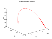
Refer to caption
(a) Dynamics, T(t)𝑇𝑡T(t), I(t)𝐼𝑡I(t), V(t)𝑉𝑡V(t)
Refer to caption
(b) Dynamics, T(t)𝑇𝑡T(t), I(t)𝐼𝑡I(t), V(t)𝑉𝑡V(t)
Refer to caption
(c) Dynamics, T(t)𝑇𝑡T(t), I(t)𝐼𝑡I(t), V(t)𝑉𝑡V(t)
Figure 2: Phase space for different values of τ𝜏\tau, which illustrates the stability of infection-free equilibrium E1subscript𝐸1E_{1}

For figure 3 we consider the following values for parameters s=8×10⁵𝑠8superscript105s=8\times 10^{5}, d=4.7×10³𝑑4.7superscript103d=4.7\times 10^{-3},μ=0.3𝜇0.3\mu=0.3, a=2𝑎2a=2, Tmax=0.7×10⁷subscript𝑇0.7superscript107T_{\max}=0.7\times 10^{7}, b=0.6×10⁷𝑏0.6superscript107b=0.6\times 10^{-7}, c=5.9𝑐5.9c=5.9, p=5.4𝑝5.4p=5.4 and α=0.001𝛼0.001\alpha=0.001, in this case the equilibrium is (7.363787665×106,1.202557883,1.100646198)7.363787665superscript1061.2025578831.100646198(7.363787665\times 10^{6},1.202557883,1.100646198) with R0=1.0014820subscript𝑅01.0014820R_{0}=1.0014820, note that this case satisfies the conditions for global stability of E2subscript𝐸2E_{2}, as is establish in theorem 4.

Refer to caption
(a) Healthy, T(t)𝑇𝑡T(t)
Refer to caption
(b) Infected, I(t)𝐼𝑡I(t)
Refer to caption
(c) Virus, V(t)𝑉𝑡V(t)
Figure 3: Stability of the infected equilibrium, E2subscript𝐸2E_{2}, with several values of τ𝜏\tau

In figure 4, we illustrate the the dynamic for system. (1) with respect to stability of infected equilibrium for several values of τ𝜏\tau.

Refer to caption
(a) Dynamics, T(t)𝑇𝑡T(t), I(t)𝐼𝑡I(t), V(t)𝑉𝑡V(t)
Refer to caption
(b) Dynamics, T(t)𝑇𝑡T(t), I(t)𝐼𝑡I(t), V(t)𝑉𝑡V(t)
Refer to caption
(c) Dynamics, T(t)𝑇𝑡T(t), I(t)𝐼𝑡I(t), V(t)𝑉𝑡V(t)
Figure 4: Phase space for different values of τ𝜏\tau, which illustrates the stability of infection equilibrium E2subscript𝐸2E_{2}

In figures 5, 6 and 7, we illustrate the stability of E2subscript𝐸2E_{2} according to theorem 5. In this case s=0.01𝑠0.01s=0.01, d=0.02𝑑0.02d=0.02, a=0.95𝑎0.95a=0.95, Tmax=1200subscript𝑇𝑚𝑎𝑥1200T_{max}=1200 b=0.0027𝑏0.0027b=0.0027 α=0.001𝛼0.001\alpha=0.001 μ=1𝜇1\mu=1, p=10𝑝10p=10, c=2.4𝑐2.4c=2.4 with this values R0=13.48subscript𝑅013.48R_{0}=13.48 , and we illustrate for different values of τ𝜏\tau. The equilibrium is (19.2,106.7,444.5)19.2106.7444.5(19.2,106.7,444.5), we can observe periodic solutions for a large value of τ𝜏\tau, also we note that the condition for the global stability of endemic equilibrium is not satisfied.
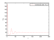
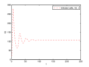
Refer to caption
(a) Healthy, T(t)𝑇𝑡T(t)
Refer to caption
(b) Infected, I(t)𝐼𝑡I(t)
Refer to caption
(c) Virus, V(t)𝑉𝑡V(t)
Figure 5: Stability of the E2subscript𝐸2E_{2} equilibrium with τ=0.1𝜏0.1\tau=0.1
Refer to caption
(a) Healthy, T(t)𝑇𝑡T(t)
Refer to caption
(b) Infected, I(t)𝐼𝑡I(t)
Refer to caption
(c) Virus, V(t)𝑉𝑡V(t)
Figure 6: Stability of the E2subscript𝐸2E_{2} equilibrium with τ=1𝜏1\tau=1
Refer to caption
(a) Healthy, T(t)𝑇𝑡T(t)
Refer to caption
(b) Infected, I(t)𝐼𝑡I(t)
Refer to caption
(c) Virus, V(t)𝑉𝑡V(t)
Figure 7: Stability of the E2subscript𝐸2E_{2} equilibrium with τ=3𝜏3\tau=3

In figure 8 we take increasing values for c𝑐c, the declination rate of virions, for the simulations we consider the values for the parameters as s=0.01𝑠0.01s=0.01, d=0.02𝑑0.02d=0.02, a=0.95𝑎0.95a=0.95, Tmax=1200subscript𝑇𝑚𝑎𝑥1200T_{max}=1200 b=0.0027𝑏0.0027b=0.0027 α=0.001𝛼0.001\alpha=0.001 μ=1𝜇1\mu=1, p=10𝑝10p=10, and τ=4𝜏4\tau=4 we can observe that for a increasing value of c=13𝑐13c=13 the periodic solutions have a smaller period and they disappear for c𝑐c large enough

Refer to caption
(a) Periodic solution for c=5𝑐5c=5
Refer to caption
(b) Periodic solution for c=10𝑐10c=10
Refer to caption
(c) Periodic solution for c=13𝑐13c=13
Figure 8: Periodic solutions for different values of c𝑐c

The numerical simulations shows that if the clearance rate of viral particles c𝑐c is sufficiently large (small) then nonexistence (existence) periodic orbits.

Now taking α=0.005𝛼0.005\alpha=0.005 we can see the effect of saturation in this case the equilibrium is (314.2,278.7,1161.2)314.2278.71161.2(314.2,278.7,1161.2) and the dynamics for different values of τ𝜏\tau are in figure 9, again we can observe periodic solutions for system.
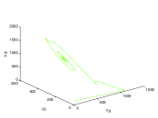
Refer to caption
(a) Dynamics, T(t)𝑇𝑡T(t), I(t)𝐼𝑡I(t), V(t)𝑉𝑡V(t), with τ=10𝜏10\tau=10
Refer to caption
(b) Dynamics, T(t)𝑇𝑡T(t), I(t)𝐼𝑡I(t), V(t)𝑉𝑡V(t), with τ=15𝜏15\tau=15
Refer to caption
(c) Dynamics, T(t)𝑇𝑡T(t), I(t)𝐼𝑡I(t), V(t)𝑉𝑡V(t), with τ=25𝜏25\tau=25
Refer to caption
(d) Dynamics, T(t)𝑇𝑡T(t), I(t)𝐼𝑡I(t), V(t)𝑉𝑡V(t), with τ=35𝜏35\tau=35
Figure 9: Dynamic of system with α=0.005𝛼0.005\alpha=0.005

8 Sensitivity analysis

In this section we provide a local sensitivity analysis of the basic reproduction number, in order to assess which parameter has the greatest influence on changes of R0subscript𝑅0R_{0} values and hence the greatest effect in determining whether the disease will be cleared in the population (see e.g. [1]).
To this aim, denoting by ΨΨ\Psi the generic parameter of system (1), we evaluate the normalised sensitivity index

SΨ=ΨR0R0Ψsubscript𝑆ΨΨsubscript𝑅0subscript𝑅0ΨS_{\Psi}=\frac{\Psi}{R_{0}}\frac{\partial R_{0}}{\partial\Psi}

which indicates how sensitive R0subscript𝑅0R_{0} is to a change of parameter ΨΨ\Psi. A positive (resp. negative) index indicates that an increase in the parameter value results in an increase (resp. decrease) in the R0subscript𝑅0R_{0} value.

We consider the values s=0.01𝑠0.01s=0.01, d=0.02𝑑0.02d=0.02, a=0.95𝑎0.95a=0.95, Tmax=1200subscript𝑇𝑚𝑎𝑥1200T_{max}=1200 b=0.0027𝑏0.0027b=0.0027 α=0.001𝛼0.001\alpha=0.001 μ=1𝜇1\mu=1, p=10𝑝10p=10, c=2.4𝑐2.4c=2.4, in order to evaluate the normalised sensitivity index, we are able to show our results in figure 10, in the figure we can appreciate that the parameters b𝑏b, p𝑝p the infection constant rate and the reproductive rate respectively have a positive influence in the value of R0subscript𝑅0R_{0} which means if we increase or decrease any of them by say 10%percent1010\% then R0subscript𝑅0R_{0} will increase or decrease by 9.9%percent9.99.9\%, note that Tmaxsubscript𝑇T_{\max} have the same effect. The index for parameters μ𝜇\mu and c𝑐c which represent the death rate of infected cells and the rate of clean of virions, show that increasing this values say by 10%percent1010\% will decrease the value of R0subscript𝑅0R_{0} almost by a 10%percent1010\%. While for the parameters a𝑎a, d𝑑d an increase of 10%percent1010\% of their value will increase and decrease respectively R0subscript𝑅0R_{0} by 2%percent22\% and 1.9%percent1.91.9\% and to increase s𝑠s by a 100%percent100100\% will increase the value of R0subscript𝑅0R_{0} by 0.8%percent0.80.8\%.

Refer to caption
Figure 10: Sensitivity index for R0subscript𝑅0R_{0} with respect to some chosen parameters

Other effects over R0subscript𝑅0R_{0} can be analyzed if we consider other values for the parameters.

9 Conclusions

In this paper, we extend the hepatitis model with mitotic transmission to incorporate the effect of saturation infection function and an intracellular time delay between infection of a infected target cell and production of new virus particles.

We have established results about the local and global stability of equilibria. We can conclude than the infection-free stability is completely determined by the value of the basic reproductive number R0subscript𝑅0R_{0}, if R01subscript𝑅01R_{0}\leq 1 then the infection-free equilibrium will be stable and unstable if R0>1subscript𝑅01R_{0}>1. For the infected equilibrium we established conditions to ensure the local stability. We need the condition ad+aTmax[T2+I2]𝑎𝑑𝑎subscript𝑇delimited-[]subscript𝑇2subscript𝐼2a\leq d+\dfrac{a}{T_{\max}}[T_{2}+I_{2}] to ensure the global stability for this equilibrium. We also established conditions for the occurrence of a Hopf Bifurcation. And we established conditions to ensure the permanence of our system. Moreover we made an estimation for the length of delay to preserve stability depending on the parameters of system (1).

For a non–cytopathic virus (d=μ𝑑𝜇d=\mu), we found the sufficient and necessary conditions of the global stability for the infected equilibrium state of hepatitis infection model (1). We note that

T2+I2=T0=Tmax2a[(ad)+(ad)2+4asTmax].subscript𝑇2subscript𝐼2subscript𝑇0subscript𝑇𝑚𝑎𝑥2𝑎delimited-[]𝑎𝑑superscript𝑎𝑑24𝑎𝑠subscript𝑇𝑚𝑎𝑥\displaystyle T_{2}+I_{2}=T_{0}=\frac{T_{max}}{2a}\left[(a-d)+\sqrt{(a-d)^{2}+\frac{4as}{T_{max}}}\right]. (27)

Substituting the relation (27) into condition ad+aTmax[T2+I2]𝑎𝑑𝑎subscript𝑇delimited-[]subscript𝑇2subscript𝐼2a\leq d+\frac{a}{T_{\max}}[T_{2}+I_{2}], we obtain

(ad)(ad)2+4asTmax.𝑎𝑑superscript𝑎𝑑24𝑎𝑠subscript𝑇𝑚𝑎𝑥\displaystyle(a-d)\leq\sqrt{(a-d)^{2}+\frac{4as}{T_{max}}}.

It is clear that the inequality is satisfied for all positive parameter values. From Theorem 4, we obtain the following corollary.

Corollary 1.

Assume that d=μ𝑑𝜇d=\mu and R0>1subscript𝑅01R_{0}>1, then the infected equilibrium state E2subscript𝐸2E_{2} of model (1) is globally asymptotically stable for any τ0𝜏0\tau\geq 0.

Our analysis shows that if the infection is not cytopathic (d=μ𝑑𝜇d=\mu) then nonexistence periodic solutions.

Acknowledgements

This article was supported by UADY under grant FMAT-2012-0004 and Mexican SNI under grants 15284 and 33365.

References

References

  • [1] G. Chowell, C. Castillo–Chavez, P.W. Fenimore, Kribs–Zaleta C. M., Arriola L., Hyman J. M., Model Parameters and Outbreak Control for SARS, Emerg. Infect. Dis., 10, 1258-–1263 (2004)
  • [2] R. V. Culshaw and S. Ruan, A delay-differential equation model of HIV infection of CD4+𝐶𝐷superscript4CD4^{+} T-cells, Math. Biosci. 165 (2000), pp. 27–39.
  • [3] R. V. Culshaw, S. Ruan and G. Webb, A mathematical model of cell-to-cell spread of HIV-1 that includes a time delay, J. Math. Biol. 46 (2003), pp. 425–444.
  • [4] H. Dahari, A. Lo, R. M. Ribeiro, A. S. Perelson, Modelling Hepatitis C virus dynamics: Liver regeneration and critical drug efficacy. J. Theor. Biol. 247, (2007), 371-381.
  • [5] H. Dahari, R. M. Ribeiro, A. S. Perelson, Triphasic decline of hepatitis C virus RNA during antiviral therapy. Hepatology 46 (2007) 16-21.
  • [6] S. Debroy, B. M. Bolker, M. Martcheva. Bistability and long-term cure in a within-host model of Hepatitis C, Journal of Biological Systems, Vol. 19, No. 4 (2011), 533-550.
  • [7] J. K. Hale, P. Waltman, Persistence in infinite-dimensional systems, SIAM J. Math. Anal. 20 (1989) 388-396.
  • [8] V. Herz, S. Bonhoeffer, R. Anderson, R. M. May, and M. A. Nowak, Viral dynamics in vivo: Limitations on estimations on intracellular delay and virus delay, Proc. Natl. Acad. Sci. USA, 93 (1996), pp. 7247–7251.
  • [9] Z. Hu, X. Liu, H. Wang, W. Ma, Analysis of the dynamics of a delayed HIV pathogenesis model, J. of Computational and Applied Mathematics, 234 (2010) pp. 461–476.
  • [10] G. Huang, Y. Takeuchi, and W. Ma, Lyapunov functionals for delay differential equations model of viral infections, SIAM J. Appl. Math., 70(7), pp. 2693–2708.
  • [11] A. Korobeinikov, Global asymptotic properties of virus dynamics models with dose-dependent parasite reproduction and virulence, and nonlinear incidence rate, Math. Medic. Biol., 26 (2009), pp. 225–239.
  • [12] Y. Kuang, Delay Differential Equations with Applications in Population Dynamics. Academic Press, San Diego 1993.
  • [13] D. Li and W. Ma, Asymptotic properties of an HIV-1 infection model with time delay, J. Math. Anal. Appl., 335 (2007), pp. 683–691.
  • [14] M. Y. Li and H. Shu, Global dynamics of an in-host viral model with intracellular delay, Bull. Math. Biol., 72 (2010), pp. 1492–1505.
  • [15] C.C. McCluskey, Complete global stability for an SIR epidemic model with delay (Distributed or discrete), Nonlinear Anal. RWA. 11 (2010) pp. 55–59.
  • [16] A. U. Neumann, N. P. Lam, H. Dahari, D. R. Gretch, T. E. Wiley, T. J. Layden, A. S. Perelson, Hepatitis C viral dynamics in vivo and the antiviral efficacy of interferon-alpha therapy. Science 282 (5386), (1998), 103-107.
  • [17] M. A. Nowak and R. M. May, Virus Dynamics: Mathematical Principles of Immunology and Virology, Oxford University Press, New York, 2000.
  • [18] A. S. Perelson and P. W. Nelson, Mathematical analysis of HIV-I dynamics in vivo, SIAM Review 41 (1999), pp. 3–44.
  • [19] R. R. Regoes, D. Ebert, and S. Bonhoeffer, Does-dependent infection rates of parasites produce the Allee effect in epidemiology, Proc. Roy. Soc. Lond. Ser. B, 269 (2002), pp. 271–279.
  • [20] S. Ruan, J. Wei, On the zeros of a third degree exponential polynomial with applications to a delayed model for the control of testosterone secretion. IMA Journal of Mathematics Applied in Medicine and Biology (2001), 18, 41-52.
  • [21] L. F. Shampine, S. Thompson, Solving DDEs in MATLAB, Appl. Numer. Math. 37 (2001) 441-458.
  • [22] X. Song, Avidan U. Neumann, Global stability and periodic solution of the viral dynamics, J. Math. Anal. Appl. 329 (2007), 281–297.
  • [23] J. Tam, Delay effect in a model for virus replication, Math. Medic. Bio., 16 (1999), pp. 29–37.
  • [24] T. F. Thingstad, T. I. Langeland, Dynamics of Chermostat Culture: The Effect of a Delay in Cell Response, J. Theor. Biol. (1974) 48, 149-159.
  • [25] C. Vargas-De-León, Global properties for virus dynamics model with mitotic transmission and intracellular delay, J. Math. Anal. Appl., 381 (2011), 884–890.
  • [26] C. Vargas-De-León, Stability analysis of a model for HBV infection with cure of infected cells and intracellular delay, Applied Mathematics and Computation 219 (2012) 389–398.
  • [27] L. Wang and S. Ellermeyer , HIV Infection and CD4+𝐶𝐷superscript4CD4^{+} T Cell Dynamics, Discrete Contin. Dyn. Syst., Ser. B 6 (2006), pp. 1417–1430.
  • [28] H. Wei, X. Li, M. Martcheva, An epidemic model of vector-borne disease with direct transmission and time delay, J. Math. Anal. Appl. 342 (2008) 895-908.
  • [29] H. Zhu and X. Zuo, Impact of delays in cell infection and virus production on HIV-1 dynamics, Math. Medic. Bio., 25 (2008), pp. 99–112.