Maximum-Likelihood Approach to Topological Charge Fluctuations
in Lattice Gauge Theory

Abstract

We present a novel technique for the determination of the topological susceptibility (related to the variance of the distribution of global topological charge) from lattice gauge theory simulations, based on maximum-likelihood analysis of the Markov-chain Monte Carlo time series. This technique is expected to be particularly useful in situations where relatively few tunneling events are observed. Restriction to a lattice subvolume on which topological charge is not quantized is explored, and may lead to further improvement when the global topology is poorly sampled. We test our proposed method on a set of lattice data, and compare it to traditional methods.

I Introduction

Lattice field theory is a powerful technique for the numerical study of Yang-Mills gauge theories. Recovery of continuum field-theory results requires extrapolations in the lattice spacing and volume, which are generally controlled and well-understood. One effect of working in a finite volume $V$ is that the theory becomes dependent on the global topological charge $Q$ Brower et al. (2003); Aoki et al. (2007). Locality and cluster decomposition properties suggest that such effects vanish as $V\rightarrow\infty$, but they must be accounted for in the extrapolation.

In Euclidean Yang-Mills quantum field theory on a torus, the topological charge $Q$ is quantized, dividing the configuration space into distinct topological sectors. These sectors are separated by an action barrier, so that the use of sampling algorithms which favor small changes in the action (such as the commonly used hybrid Monte Carlo algorithm) can lead to poor sampling of this distribution. Since the action barrier can grow with decreasing lattice spacing Alles et al. (1996); Del Debbio et al. (2004); Lüscher (2010) or increasing number of flavors $N_{f}$ Appelquist et al. (2010, 2012), the cost of tunneling to different topological sectors can vary greatly depending on the details of the calculation.

The “freezing” of topological charge resulting from these algorithmic problems leads to extremely long autocorrelation times, so that the distribution of $Q$ is poorly sampled. Correction of the resulting systematic effects on observables can be done Brower et al. (2003); Aoki et al. (2007), but these corrections require as inputs the cumulants of the topological charge distribution, particularly the variance $\langle Q^{2}\rangle\equiv V\chi_{t}$, where $\chi_{t}$ is the topological susceptibility. Using the standard estimator for variance requires many independent samples; autocorrelations can lead to relatively few independent measurements and a biased estimate with a large sampling error.

In this work, we suggest two ways to proceed when confronted with this problem. First, it is generally believed that the maximum likelihood (ML) method (see Sec. 36.1.2 of Beringer et al. (2012)) can produce reliable estimates of model parameters when there are relatively few independent samples of a distribution, provided the functional form of the underlying distribution is known analytically. Inspired by the work of Phil Nelson and collaborators Beausang et al. (2011), we present such a maximum likelihood approach (following an example by Franco Franco, José Carlos Garcıa (2003) in the context of financial time-series) to analyze the complete time-series information $\{Q_{n}\}$. The analysis is done without blocking, since the effect of autocorrelations is built into the model. This method in principle allows the estimation of $\chi_{t}$ from even a handful of tunneling events.

Eventually, if one performs a calculation at sufficiently small (but finite) lattice spacing Lüscher (1982), global topological charge will never change in any finite number of Markov steps. If we choose a lattice volume $V$ such that $V\chi_{t}\gg 1$, we can consider the distribution of topological charge $Q_{s}$ computed only in subvolumes $V_{s}\gg\chi_{t}^{-1}$, which by locality and cluster decomposition should also be distributed asymptotically as the stationary distribution $P(Q)$. In this scenario, we can employ either our ML method or a more standard blocked sample variance estimate to compute the susceptibility, depending on the number of independent samples . Empirically, we find that the calculation of $\chi_{t}$ based on a subvolume gives the most robust estimates of $\chi_{t}$ in the case that relatively few uncorrelated measurements of $Q$ are available, although further study of this approach is needed.

The contents of this manuscript are as follows: in section II we discuss what is known about the distribution of topological charge in lattice simulations of Yang-Mills gauge theories. Section III gives the definition of an Ornstein-Uhlenbeck (OU) process, which uniquely describes continuous Markov processes that remain Gaussian distributed. Section IV describes the maximum-likelihood estimation of $\chi_{t}$ based on the OU model. In section V, the implications of studying calculations with nearly-fixed global topological charge are discussed, and a modification of the maximum-likelihood estimate using lattice subvolumes is introduced. Section VI demonstrates the use of the proposed methods to extract $\chi_{t}$ on an example set of lattice configurations, and compares to other standard approaches. Finally, section VII summarizes our results and discusses future applications and possible improvements.

II Distribution of topological charge

Numerical lattice computations make use of a Markov process to sample the configuration space, generating a sequence of configurations $U_{0}\to U_{1}\to\cdots\to U_{n}$ with corresponding topological charges $\{Q_{n}\}$. As the sample size $n$ increases, the distribution $P(Q_{n})$ converges to a stationary distribution $P(Q)$.

What is known about the distribution $P(Q)$? With zero $\theta$-parameter, all odd cumulants of the distribution must vanish by parity invariance. Furthermore, analysis of SU$(N_{c})$ gauge theories at large-$N_{c}$ shows that the even cumulants scale as $\kappa_{2n}\sim N_{c}^{2-2n}$ ’t Hooft (1974); Witten (1979, 1980), suggesting that the distribution will be approximately Gaussian. Given the suppression of higher cumulants, it seems reasonable to express the distribution $P(Q)$ in terms of its Edgeworth series Blinnikov and Moessner (1998), truncated to the first non-Gaussian term:

$$P(Q)=\frac{32}{32+\epsilon}P_{G}\left(\frac{Q}{\sqrt{\sigma}}\right)\left[1+\frac{\epsilon}{4!}\mathrm{He}_{4}\left(\frac{Q}{\sqrt{\sigma}}\right)\right],$$ (1)

where $P_{G}(x)$ is the Gaussian distribution with zero mean and unit variance and $\mathrm{He}_{4}(x)=x^{4}-6x^{2}+3$ is a Hermite polynomial. The variance $\kappa_{2}$ and 4th-order cumulant $\kappa_{4}$ for this distribution are

$$\kappa_{2}=\sigma^{2}\left(1+\frac{\epsilon}{4}\right)+O(\epsilon^{2}),\quad\frac{\kappa_{4}}{\kappa_{2}^{2}}=\epsilon+O(\epsilon^{2}).$$ (2)

We identify the variance $\langle Q^{2}\rangle=\kappa_{2}\equiv V\chi_{t}$, which defines the topological susceptibility $\chi_{t}$. As $\epsilon\rightarrow 0$, this distribution becomes purely Gaussian; several lattice studies have empirically found non-zero $\epsilon$ in SU$(N_{c})$ gauge theories D’Elia (2003); Del Debbio et al. (2006); Durr et al. (2007); Giusti et al. (2007); Bonati et al. (2013). We note that the dependence of this non-Gaussianity on the presence of light fermions is unclear, and large-$N_{c}$ arguments may be inapplicable for theories with many fermions $N_{f}$, unless $N_{f}/N_{c}$ is held fixed as $N_{c}\rightarrow\infty.$

III Ornstein-Uhlenbeck process

We wish to consider Markov processes that can reproduce the approximately-Gaussian topological charge distribution eq. 1. In fact, up to linear transformations in the variables, there is a unique non-trivial example of a continuous Markov process in which the expected distribution at any point in the stochastic evolution is Gaussian: the Ornstein-Uhlenbeck (OU) process Uhlenbeck and Ornstein (1930); Doob (1942), which describes the Brownian motion of a massive particle in the presence of arbitrary linear friction. This process is described by the stochastic differential equation

$$\frac{d}{dt}x(t)=-\eta\left(x(t)-\overline{x}\right)+\sigma\frac{d}{dt}W(t)$$ (3)

where $\eta>0$, $\sigma>0$ and $W(t)$ is the stochastic Wiener process of Brownian motion. The standard solution leads to the following statistics:

$$\mathrm{E}[x(t)] = \overline{x}+\left(x(0)-\overline{x}\right)e^{-\eta t}$$

$$\mathrm{Var}[x(t)] = \frac{\sigma^{2}}{2\eta}\left(1-e^{-2\eta t}\right)$$ (4)

which converge to a Gaussian with mean $\bar{x}$ and variance $\sigma^{2}/2\eta$ as $t\rightarrow\infty$, independent of the starting position $x(0)$. We will discuss the accuracy of this model in the presence of small non-Gaussianities in section IV below.

The detailed evolution of topological charge in a lattice gauge theory calculation is quite complex and dependent on unphysical details such as the choice of the update algorithm. Since it is a Markov process and since $Q$ is distributed as a Gaussian asymptotically (up to corrections which we will discuss), we will model the evolution of topological charge as an OU process.

The friction parameter $\eta$ is sensitive to algorithmic details and therefore not physically relevant, so it will be treated as a nuisance parameter. Although we will not investigate it in detail here, we note that the parameter $\eta$ may be of interest in the comparison of different lattice update algorithms (with the underlying physical parameters held fixed). In particular, the autocorrelation $R(\tau)$ for the process $x(t)$ from the standard solution is given by

$$R(\tau)=e^{-\eta\tau}\left(\frac{1-e^{-2\eta(t+\tau)}}{\sqrt{(1-e^{-2\eta t})(1-e^{-2\eta(t+\tau)})}}\right)$$ (5)

which for $t\gg 1/\eta$ converges to $e^{-\eta\tau}$. We can therefore identify $1/\eta$ as the standard autocorrelation time for $x$. Our approach to be described below therefore gives an alternate way to estimate the autocorrelation time for an observable which is expected to always be approximately Gaussian distributed.

IV Maximum Likelihood Estimate

We assume that we have $N+1$ computations of the topological charge $Q_{i}$ at steps $n_{i}$ in the Markov chain, where the $n_{i}$ need not be equally spaced. Due to parity invariance of Yang-Mills theory, all odd moments are identically zero, including the mean $\langle Q\rangle=0$. The second moment, or equivalently the variance, gives the topological susceptibility

$$\langle Q^{2}\rangle=V\chi_{t}.$$ (6)

In the OU model, we identify the susceptibility in terms of the model parameters, $V\chi_{t}=\sigma^{2}/2\eta$. The conditional probability of finding $Q_{i}$ at step $n_{i}$ given $Q_{i-1}$ was found at step $n_{i-1}$ is Gaussian with mean and variance given by Eq. (4) with appropriate asymptotic values:

$$P(Q_{i}|Q_{i-1})$$ (7)

$$= (2\pi)^{-\frac{1}{2}}\left[V\chi_{t}\left(1-e^{-2\eta(n_{i}-n_{i-1})}\right)\right]^{-\frac{1}{2}}$$

$$\times\exp\left\{-\frac{\left[Q_{i}-Q_{i-1}e^{-\eta(n_{i}-n_{i-1})}\right]^{2}}{2V\chi_{t}\left[1-e^{-2\eta(n_{i}-n_{i-1})}\right]}\right\}\ .$$

The log-likelihood function (dropping additive constants) given the time series is

$$L(\eta,V\chi_{t}) = -\frac{N}{2}\log V\chi_{t}-\frac{1}{2V\chi_{t}}S(\eta)$$ (8)

$$-\frac{1}{2}\sum_{i=1}^{N}\log\left[1-e^{-2\eta(n_{i}-n_{i-1})}\right]$$

where for later convenience we have defined the sum

$$S(\eta)\equiv\sum_{i=1}^{N}\frac{\left[Q_{i}-Q_{i-1}e^{-\eta(n_{i}-n_{i-1})}\right]^{2}}{1-e^{-2\eta(n_{i}-n_{i-1})}}\ .$$ (9)

The maximum likelihood (ML) estimates $\widehat{\eta}$ and $\widehat{\chi}_{t}$ minimize the log-likelihood function $L(\eta,V\chi_{t})$. At the minimum,

$$\left.\frac{\partial L(\eta,V\chi_{t})}{\partial V\chi_{t}}\right|_{V\widehat{\chi}_{t}}=0$$ (10)

which leads to

$$V\widehat{\chi}_{t}=\frac{1}{N}S(\widehat{\eta})\ .$$ (11)

If we substitute $S(\eta)/N$ for $V\chi_{t}$ in the log-likelihood function we now need to solve the one-dimensional problem to find $\widehat{\eta}$ that minimizes

$$\mathcal{L}(\eta)=-\frac{N}{2}\log S(\eta)-\frac{1}{2}\sum_{i=1}^{N}\log\left[1-e^{-2\eta(n_{i}-n_{i-1})}\right]$$ (12)

where we have dropped further additive constants. Once $\widehat{\eta}$ is known then $V\widehat{\chi}_{t}$ is known as well.

Figure 1: Monte Carlo test of variance extracted from an Edgeworth distribution eq. 1, as a function of non-Gaussianity parameter $\epsilon$. The dashed line (black) shows the analytic variance vs. $\epsilon$. The points with error bars (blue) and the shaded band (red) show estimated variance using the sample variance and OU maximum-likelihood estimate, respectively. Both methods show good agreement with the expected variance.

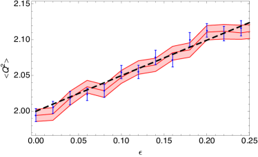
Since the OU model assumes the underlying distribution is Gaussian, it is interesting to understand how well the OU-model ML estimates can reproduce the variance of the nearly Gaussian distribution in Eq. (1) for $\epsilon\approx 0.2$ Giusti et al. (2007). As a simple test, we generated 100,000 samples of the distribution for $\sigma^{2}=2$ and $\epsilon=0\text{--}0.24$ and used both the OU ML method and the standard sample variance to estimate $\langle Q^{2}\rangle$. Both estimates agree well with the analytic value, as shown in fig. 1. In addition, near-perfect agreement is seen between the OU model and the standard sample variance, for this test in which the underlying true distribution is near-Gaussian and well-sampled.

V NEARLY FIXED TOPOLOGY

For lattice calculations in which the topological charge tunnels frequently, the distribution of $Q$ will be well-sampled, and $\chi_{t}$ can be estimated simply from the empirical sample variance, or from a least-squares (LS) fit of a Gaussian to the $Q$ distribution. The advantage of the ML method is that it should still yield robust estimates of $\chi_{t}$ even when the distribution is relatively poorly sampled. However, in extreme cases where the number of observed tunneling events is $O(10)$ or less, the uncertainty in $\chi_{t}$ can become very large, as a lack of tunneling events can be explained by either large $\chi_{t}$ and small $\eta$, or vice-versa. Marginalizing over $\eta$ leads to essentially a lower bound on $\chi_{t}$.

Recently, it has been suggested that the use of Neumann boundary conditions along one of the directions of the lattice would eliminate the barrier to changing topology Lüscher and Schaefer (2011). One can think rather informally of this scenario as topological charge being allowed to flow freely through the boundaries between the lattice and an infinite reservoir. This physical picture suggests an alternative approach to estimation of $\chi_{t}$.

Consider a periodic lattice with volume $V=L^{3}\times T$ and $T\gg L$, and then select some contiguous interval of length $T_{s}\ll T$, such that $V\gg V_{s}\equiv L^{3}\times T_{s}\gg\chi_{t}^{-1}$. The total topological charge $Q_{s}$ contained within this subvolume $V_{s}$ will be a continuous variable, since charge is no longer conserved; it can move freely into the complement of $V_{s}$, which we can think of as a reservoir.

The existence of a non-zero global topological charge $Q$ on the full volume may bias the distribution of charge within the subvolume; in particular, if $Q$ is fixed, then the mean charge contained within $V_{s}$ will be equal to $QV_{s}/V$. We therefore define a “subtracted” subvolume charge,

$$\mbox{$Q_{s,\textrm{sub}}$}=\int_{x\in V_{s}}d^{4}x\left[q(x)-\frac{Q}{V}\right]$$ (13)

where $q(x)$ is the topological charge density at lattice site $x$. We then carry out the analysis exactly as before, but with the substitutions $V\rightarrow V_{s}$ and $Q\rightarrow Q_{s,\textrm{sub}}$.

It seems reasonable, although not proven, that $\chi_{t}$ computed this way is an acceptable estimator of topological susceptibility when using the methods suggested in Brower et al. (2003), given that $V$ was periodic and translationally invariant and $V_{s}$ was chosen at random. Thus, we can apply our same ML method to a time series in $Q_{s}$ to get an estimate of $V_{s}\chi_{t}$. Even with nearly-fixed $Q$, it may be possible for $Q_{s}$ to fluctuate frequently enough to allow a reliable LS fit. In this case, we can check that ML and sample variance methods produce compatible results for $V_{s}\chi_{t}$.

VI EXAMPLES

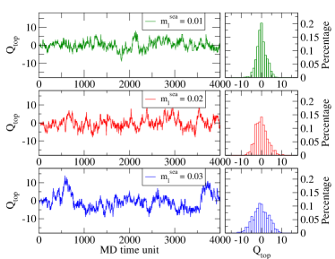
As a trial of this method, we take a few time series of topological charge on a set of three $16^{3}\times 32$ lattice ensembles with $N_{f}=2$+1 domain wall fermions, generated by the RBC and UKQCD collaborations Allton et al. (2007). The relevant data and empirical distributions of $Q$ are plotted in fig. 2. For the analysis to follow we take a thermalization cut of 200 MD time units on all three ensembles. The topological charge is measured every 5 MD time units.

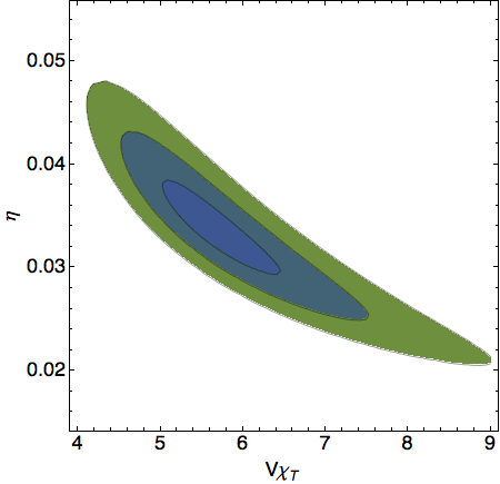
In Fig. 3, for the lightest mass $m_{l}=0.01$ ensemble we show the $2\Delta L=1,4,9$ contours appropriate for estimating the 1, 2, 3 $\sigma$ confidence intervals on $V\chi_{t}$ while marginalizing over the friction parameter $\eta$. The resulting 1-$\sigma$ confidence interval on $V\chi_{t}$ is found to be in good agreement with the standard sample-variance estimate.

The negative correlation between $V\chi_{t}$ and $\eta$ is expected, since they are inversely related through the asymptotic variance of the model distribution, $V\chi_{t}=\sigma^{2}/2\eta$. For data sets with relatively few tunneling events, we expect the ellipsoid will become elongated and follow a hyperbolic curve due to this relation.

Figure 2: From Allton et al. (2007), Markov-chain Monte Carlo time-series (left) and cumulative distributions (right) of global topological charge $Q$, as measured by the RBC and UKQCD collaborations. Three ensembles are shown, differing by the light-quark mass: $m_{l}=0.01$ (top), 0.02 (middle), and 0.03 (bottom).

Figure 3: Confidence contours for maximum likelihood analysis of the RBC/UKQCD $m_{l}=0.01$ ensemble, shown at $1\sigma$, $2\sigma$, and $3\sigma$ levels.

We would now like to test the proposed subvolume analysis of section V, in conjunction with both the sample variance and ML methods. The use of only a fixed subvolume from all configurations would reduce the available statistics, so we make use of a bootstrap procedure in order to improve our statistical precision. We draw $N_{b}=1000$ bootstrap replications from the distribution of pairs $\{Q_{i},Q_{i+1}\}$ in the topological charge time series, allowing us to resample while preserving the information on transitions required by the ML method. We fix the subvolume size $T_{s}\leq T$, and then within each bootstrap replication choose a random starting position $t\in[0,N_{t}-1]$ for the subvolume on each configuration in the timeseries; the choice is randomized for each bootstrap replication. This procedure imposes the expected translation invariance in the $t$-direction.

For the sample variance procedure, the data are blocked before drawing bootstrap samples, in order to deal with autocorrelation effects. Empirical tests on the data show stability of error estimates on $\chi_{t}$ for a block length of roughly $\sim 100$ trajectories or 20 configurations. No blocking is used for the ML analysis, which includes autocorrelation effects in the model. For both the sample variance and ML subvolume analyses, the central value and error estimates correspond to the median and one-sigma quantiles of the bootstrap distribution, respectively.

Figure 4: Comparison of various methods for determination of $V\chi_{t}$ on the three RBC/UKQCD example ensembles studied. “SV” denotes use of the sample variance of $Q$, while “ML” indicates the maximum-likelihood method described in the text. “Subvol” indicates analysis restricted to a subvolume with full spatial extent and $T_{s}=8$.

$V\chi_{t}$	$m_{l}=0.01$	0.02	0.03
SV	5.68$\left(\begin{smallmatrix}+91\\ -84\end{smallmatrix}\right)$	9.19$\left(\begin{smallmatrix}+1.23\\ -1.16\end{smallmatrix}\right)$	16.86$\left(\begin{smallmatrix}+3.10\\ -2.96\end{smallmatrix}\right)$
ML	5.64$\left(\begin{smallmatrix}+82\\ -66\end{smallmatrix}\right)$	9.40$\left(\begin{smallmatrix}+1.47\\ -1.14\end{smallmatrix}\right)$	17.18$\left(\begin{smallmatrix}+3.73\\ -2.70\end{smallmatrix}\right)$
SV subvol	7.44$\left(\begin{smallmatrix}+43\\ -41\end{smallmatrix}\right)$	10.26$\left(\begin{smallmatrix}+71\\ -66\end{smallmatrix}\right)$	13.32$\left(\begin{smallmatrix}+1.30\\ -1.20\end{smallmatrix}\right)$
ML subvol	7.38$\left(\begin{smallmatrix}+1.16\\ -0.87\end{smallmatrix}\right)$	10.24$\left(\begin{smallmatrix}+1.71\\ -1.22\end{smallmatrix}\right)$	13.38$\left(\begin{smallmatrix}+2.38\\ -1.75\end{smallmatrix}\right)$

Table 1: Comparison of various methods for determination of $V\chi_{t}$ on the three RBC/UKQCD example ensembles studied. “SV” denotes use of the sample variance of $Q$, while “ML” indicates the maximum-likelihood method described in the text. Rows labeled “subvol” apply the same techniques on a subvolume with full spatial extent and $T_{s}=8$.

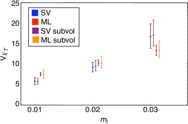
In Fig. 4 and table 1, we summarize our determination of $V\chi_{t}$ for the three ensembles shown in Fig. 2 using the various methods described. The subvolume results here are for fixed $T_{s}=8$. As expected from a time series with many independent samples of $P(Q)$, the maximum likelihood (ML) result agrees closely with the sample variance (SV) estimate of $V\chi_{t}$.

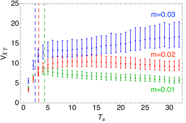
We further investigate the subvolume estimates, and in particular their dependence on the choice of subvolume size, by varying the temporal extent $T_{s}$ and repeating the analysis. The results are shown for all three ensembles in fig. 5. A strong variation is seen at small $T_{s}$, setting in approximately where $V_{s}\chi_{t}\approx 1$, which is where our assumptions about the simplicity of the distribution $P(Q)$ are anticipated to break down. For large $T_{s}$ the dependence on subvolume size is nearly flat, but with a small systematic trend evident, particularly on the $m_{l}=0.03$ ensemble. We have no immediate physical explanation for the origin of this subleading effect, but plan to investigate further in a future work.

Figure 5: Dependence of ML subvolume estimates of $V\chi_{t}$ on the temporal extent of the $L^{3}\times T_{s}$ subvolume used, for the three RBC/UKQCD example ensembles, from bottom to top $m_{l}=0.01$ (green), $0.02$ (red) and $0.03$ (blue). The vertical lines show the point at which $V_{s}\chi_{t}\approx 1$ on each ensemble (based on the ML estimate at $T_{s}=8$), beyond which our method is expected to break down.

Figure 6: Comparison of estimates of topological susceptibility times the volume $V\chi_{t}$ taken on a subset of the RBC $m_{l}=0.01$ gauge configurations, with MD trajectory numbers up to $\tau_{\textrm{max}}$. Points shown correspond to different methods: sample variance (blue), maximum likelihood (red), subvolume SV (purple), and subvolume ML (orange). All SV-method results are shown with an offset for clarity. Subvolume ML estimates (again with $T_{s}=8$) show the best consistency with the “asymptotic” result (black band) obtained by the ML method applied to the full time series.

It is apparent that the ML method does not offer any significant advantage in the determination of $V\chi_{t}$ over a simple calculation of the sample variance when the underlying distribution $P(Q)$ is well-sampled, as is the case for the full time series on each of the RBC ensembles. However, we expect the ML technique to be a robust approach even when a small number of independent samples are available. Furthermore, even when the distribution is well-sampled, the ML method has the advantage of including autocorrelation effects automatically, into the friction parameter $\eta$, whereas the SV analysis requires an autocorrelation analysis and blocking to be carried out first.

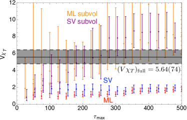
We can test what might happen in a case with poor sampling by analyzing a restricted subset of the RBC time series. Fig. 6 shows the results of this test on the $m_{l}=0.01$ ensemble, with the analysis considered on the restricted time series with MD time $\tau\leq\tau_{\textrm{max}}$; as a reminder, $Q$ is measured every 5 MD time units. For the SV analysis, we adjust the blocking when only a small number of configurations are available; specifically, we use a block length of $\tau=50$ when less than $200$ time units are available, and $\tau=25$ for less than $100$ time units available. With only a subset of the configurations, the full-volume methods show a clear bias with respect to the best estimate of $V\chi_{t}$ from the full ensemble. On the other hand, both the ML and SV subvolume approaches converge rapidly to cover the asymptotic estimate, with the ML being particularly effective at small $\tau_{\textrm{max}}$ where a simple blocking analysis cannot adequately account for the known autocorrelation effects.

VII Discussion

We have introduced a new maximum-likelihood approach to estimation of the topological susceptibility $\chi_{t}$ in lattice calculations, based on maximum-likelihood analysis of the full time-series information. This approach can give an advantage over more traditional methods such as calculation of the sample variance of $Q$, particularly in the case that autocorrelation times are long and relatively few independent samples are available, due to the inclusion of autocorrelation effects within the ML model. The autocorrelation time of $Q$ can also be estimated as a byproduct of the analysis.

In addition, we have explored the analysis of topological charge fluctuations on lattice subvolumes. This technique may be necessary in cases where the global topological charge goes through few or even no tunneling events within a lattice calculation. Even when $Q$ fluctuates adequately, the subvolume method (in conjunction with the ML analysis) was found to give the most robust estimates of $\chi_{t}$, with confidence intervals rapidly converging to cover the asymptotic estimates of this quantity even on small amounts of data. Stability of the estimate with respect to the subvolume size was observed empirically down to $V_{s}\chi_{t}\approx 1$, at which point our physical assumptions about the fluctuations should break down.

A modification of the ML approach to a more complex model than the OU process, which might be able to deal with non-Gaussian distributions and therefore extract higher moments by the maximum-likelihood approach, would be interesting to study in a future work. The modeling of higher-order systematic dependence on the subvolume size, as hinted at by our current analysis, also merits further study.

We thank the RBC-UKQCD collaboration for the use of their lattice configurations, first published in Ref. Allton et al. (2007), and we also thank Tom Blum and Philippe de Forcrand for useful discussions. This work was supported in part by the National Science Foundation under Grant No. PHYS-1066293 and the hospitality of the Aspen Center for Physics. M.L. was partially supported by SciDAC-3 and Argonne Leadership Computing Facility at Argonne National Laboratory under contract DE-AC02-06CH11357, and the Brookhaven National Laboratory Program Development under grant PD13-003. D.S. was supported by DOE Grant Nos. DE-SC0010005, DE-SC0008669 and DE-SC0009998. R. C. B., C. R., and E. W. were supported by DOE grant DE-SC0010025. In addition, R. C. B., C. R., M. C. and O. W. acknowledge the support of NSF grant OCI-0749300, and G. F. and G. V. were supported by NSF grant PHY11-00905. We thank LLNL for funding from LDRD13-ERD-023, and E. R., C. S., and P. V. acknowledge the support of the U. S. Department of Energy under Contract DE-AC52-07NA27344 (LLNL).

References

- Brower et al. (2003) R. Brower, S. Chandrasekharan, J. W. Negele, and U. Wiese, Phys.Lett. B560, 64 (2003), eprint hep-lat/0302005.
- Aoki et al. (2007) S. Aoki, H. Fukaya, S. Hashimoto, and T. Onogi, Phys.Rev. D76, 054508 (2007), eprint 0707.0396.
- Alles et al. (1996) B. Alles, G. Boyd, M. D’Elia, A. Di Giacomo, and E. Vicari, Phys.Lett. B389, 107 (1996), eprint hep-lat/9607049.
- Del Debbio et al. (2004) L. Del Debbio, G. M. Manca, and E. Vicari, Phys.Lett. B594, 315 (2004), eprint hep-lat/0403001.
- Lüscher (2010) M. Lüscher, JHEP 1008, 071 (2010), eprint 1006.4518.
- Appelquist et al. (2010) T. Appelquist et al. (LSD Collaboration), Phys.Rev.Lett. 104, 071601 (2010), eprint 0910.2224.
- Appelquist et al. (2012) T. Appelquist, R. C. Brower, M. I. Buchoff, M. Cheng, S. D. Cohen, et al. (2012), eprint 1204.6000.
- Beringer et al. (2012) J. Beringer et al. (Particle Data Group), Phys.Rev. D86, 010001 (2012).
- Beausang et al. (2011) J. F. Beausang, Y. E. Goldman, and P. C. Nelson, Meth.Enzymol. 487, 431 (2011).
- Franco, José Carlos Garcıa (2003) Franco, José Carlos Garcıa, Real Options Practice (2003), URL http://www.investmentscience.com/Content/howtoArticles/MLE_for_OR_mean_reverting.pdf.
- Lüscher (1982) M. Lüscher, Commun.Math.Phys. 85, 39 (1982).
- ’t Hooft (1974) G. ’t Hooft, Nucl.Phys. B72, 461 (1974).
- Witten (1979) E. Witten, Nucl.Phys. B149, 285 (1979).
- Witten (1980) E. Witten, Annals Phys. 128, 363 (1980).
- Blinnikov and Moessner (1998) S. Blinnikov and R. Moessner, Astron.Astrophys.Suppl.Ser. 130, 193 (1998), eprint astro-ph/9711239.
- D’Elia (2003) M. D’Elia, Nucl.Phys. B661, 139 (2003), eprint hep-lat/0302007.
- Del Debbio et al. (2006) L. Del Debbio, G. M. Manca, H. Panagopoulos, A. Skouroupathis, and E. Vicari, JHEP 0606, 005 (2006), eprint hep-th/0603041.
- Durr et al. (2007) S. Durr, Z. Fodor, C. Hoelbling, and T. Kurth, JHEP 0704, 055 (2007), eprint hep-lat/0612021.
- Giusti et al. (2007) L. Giusti, S. Petrarca, and B. Taglienti, Phys.Rev. D76, 094510 (2007), eprint 0705.2352.
- Bonati et al. (2013) C. Bonati, M. D’Elia, H. Panagopoulos, and E. Vicari, Phys.Rev.Lett. 110, 252003 (2013), eprint 1301.7640.
- Uhlenbeck and Ornstein (1930) G. Uhlenbeck and L. Ornstein, Phys.Rev. 36, 823 (1930).
- Doob (1942) J. L. Doob, Ann. Math. 43, 351 (1942).
- Lüscher and Schaefer (2011) M. Lüscher and S. Schaefer, JHEP 1107, 036 (2011), eprint 1105.4749.
- Allton et al. (2007) C. Allton et al. (RBC Collaboration, UKQCD Collaboration), Phys.Rev. D76, 014504 (2007), eprint hep-lat/0701013.
- de Forcrand et al. (1999) P. de Forcrand, M. Garcia Perez, J. Hetrick, E. Laermann, J. Lagae, et al., Nucl.Phys.Proc.Suppl. 73, 578 (1999), eprint hep-lat/9810033.