Analysis of Push-type Epidemic Data Dissemination in Fully Connected Networks

Abstract

Consider a fully connected network of nodes, some of which have a piece of data to be disseminated to the whole network. We analyze the following push-type epidemic algorithm: in each push round, every node that has the data, i.e., every infected node, randomly chooses $c\in{\mathbb{Z}}_{+}$ other nodes in the network and transmits, i.e., pushes, the data to them. We write this round as a random walk whose each step corresponds to a random selection of one of the infected nodes; this gives recursive formulas for the distribution and the moments of the number of newly infected nodes in a push round. We use the formula for the distribution to compute the expected number of rounds so that a given percentage of the network is infected and continue a numerical comparison of the push algorithm and the pull algorithm (where the susceptible nodes randomly choose peers) initiated in an earlier work. We then derive the fluid and diffusion limits of the random walk as the network size goes to $\infty$ and deduce a number of properties of the push algorithm: 1) the number of newly infected nodes in a push round, and the number of random selections needed so that a given percent of the network is infected, are both asymptotically normal 2) for large networks, starting with a nonzero proportion of infected nodes, a pull round infects slightly more nodes on average 3) the number of rounds until a given proportion $\lambda$ of the network is infected converges to a constant for almost all $\lambda\in(0,1)$. Numerical examples for theoretical results are provided.

Keywords: peer to peer; pull; push; epidemics ; epidemic algorithm ; diffusion ; fluid ; approximation ; asymptotic ; analysis ; data dissemination ; fully connected ; network ; graph

1 Introduction

Epidemic algorithms mimic spread of infectious diseases to disseminate data in large networks [8, 18, 12, 17, 20, 21, 25]. As is common in the literature, let us call a node of a network infected if it holds the piece of data to be disseminated and susceptible otherwise. Two of the main types of epidemic algorithms are push and pull. Both of these progress in discrete stages called rounds; in a push round, each infected node randomly selects $c>0$ nodes uniformly and without repetition among the rest of the nodes and uploads, i.e, pushes, the data to these nodes; in a pull round, each susceptible node randomly selects $c$ nodes and if any of these nodes is infected, the selecting node downloads, i.e., pulls, the data from the infected node to which it has connected. The parameter $c$ is called the fanout.

One calls a network fully connected if each of its nodes can directly connect to any other node in the network. If the network is represented as a graph, the network is fully connected if and only if its graph is complete. Analysis over fully connected networks is a natural first step in the study of algorithms on networks. [17, 21, 13, 5] study epidemic algorithms on fully connected networks and [15, 4, 9] study a range of other stochastic algorithms on them; see Section 5 for more on fully connectedness and for comments on other topologies. The aim of the present work is a thorough analysis of the push algorithm over fully connected networks; the following paragraphs explain the elements of this analysis.

A key random variable in epidemic algorithms is the number $Y$ of newly infected nodes after an epidemic round. The paper [19] studies this random variable for fully connected networks and observes that it is binomial for the pull round when conditioned on the number of infected nodes in the network right before the round begins. For the distribution of $Y$ in the push round, [19] assumes $c=1$ and derives the formula (2.1) by counting all digraphs which correspond to each realization of $Y$. The direct computation of (2.1) requires high precision and lengthy arithmetic and this restricts its use to small networks $(n\leq 200)$. In Section 2 we take a different route and represent $Y$ for general $c$ using a random walk $S$ with linear and state dependent dynamics. Recall that within a push round each infected node randomly selects $c$ peers and transmits its data to these peers. Each step of the walk $S$ corresponds to one of these random selections; see (2.2), (2.3) and (2.6) for the exact dynamics. The position $S_{k}$ of the walk at its $k^{th}$ step ($k$ being the number of infected nodes before the round begins) is our desired representation of $Y$. Subsection 2.1 explains how $S$ can be used as a model for the whole push algorithm when it is allowed to take an unlimited number of steps. The next subsection computes the first and second moments of $S$, which gives, in particular, those of $Y$.

The random walk $S$ is also a discrete time Markov chain and its dynamics therefore can be expressed as its one step transition matrix $P$. Thus, one can write (for all $n$, $k$ and $c$) the distribution of $Y$ as the first row of $P^{k}$. This gives a fast algorithm to compute $Y$’s distribution for small $c$, because $P$ is sparse when $c$ is small. Section 3 uses this algorithm to compute for $n=500$, and $c\in\{1,7\}$, the expected number of push rounds needed so that the proportion of the infected nodes in the network reaches $\lambda\in(0,1)$. This expectation is simple to compute for the pull algorithm, because $Y$ of that algorithm is binomial. Figures 2 and 3 compare the aforementioned expectation for the push and the pull algorithms.

Section 4 contains the main results of our analysis: here we compute the diffusion and fluid limits of the random walk $S$ and derive a number of properties of the push epidemic algorithm from these limits. For the asymptotic analysis to make sense we set the initial number of infected nodes to $k_{n}$ such that $\lim_{n}k_{n}/n=(1-\mu)\in(0,1).$ Theorem 1 shows that as $n$ goes to $\infty$, the scaled random walk $S/n$ behaves like $t\rightarrow\Gamma_{t}+\frac{1}{\sqrt{n}}X_{t}$ where $\Gamma$ is the deterministic process $t\rightarrow\mu(1-e^{-ct})$ and $X$ is a time discounted Wiener integral of a function of $\Gamma$ (see (4.23)). The $t$ variable here is the continuous scaled time and $t=(1-\mu)=\lim_{n}k_{n}/n$ corresponds to the ${k_{n}}\approx(1-\mu)n^{th}$ step of the random walk and hence to the end of the first push round. This establishes that $\sqrt{n}(Y/n-\Gamma_{1-\mu})$ converges to a zero mean normal random variable whose variance is given by the quadratic variation of $X$ ((4.26) and (4.27)). Subsection 4.1 uses Theorem 1 to compare the pull and the push algorithms for large fully connected networks. In particular, (4.29) says that a pull round always infects slightly more nodes on average, for large networks and starting with a nonzero proportion of infected nodes. The difference disappears as $c$ increases. When the network is initially half infected, for $c>15$ a single round of push or pull suffices to infect almost all of the nodes.

The last observation suggests that one study more carefully what happens in a single round. The random walk representation and its limits allow exactly this. In subsection 4.2 we use the asymptotic limit of $S$ derived in Theorem 1 to compute the asymptotics of the number $\tau^{n}_{\lambda}$ of random selections needed so that the proportion of infected nodes in the network reaches $\lambda\in(0,1)$. Theorems 2 and 3 say that this quantity is also asymptotically normal and provide its mean and variance. $\tau^{n}_{\lambda}$ is not a function of the value of $S$ at a particular deterministic point in time but of its whole path. Thus, a stochastic process level analysis of $S$ is inevitable in the study of $\tau^{n}_{\lambda}$.

Subsection 4.3 uses $\Gamma$ to derive the fluid limit of a sequence of push rounds. Let us denote by $\nu_{\lambda}^{n}$ the (random) number of push rounds needed so that the proportion of the network is above $\lambda\in(0,1).$ The final result of our analysis is Theorem 4, which says that as the network size increases to $\infty$, $\nu_{\lambda}^{n}$ converges to a constant integer, if $\lambda$ is not one of the deterministic levels derived in subsection 4.3 that the fluid limit of the rounds go through.

Although we have not seen in the prior literature the diffusion analysis of the random walk $S$, the proof of Theorem 1 is based on results and ideas in [11] and is relegated to the appendix. We have not been able to find in the prior literature analyses and proofs similar to the ones we give in subsections 4.2 and 4.4 and therefore the proofs in these subsections follow the statements of the theorems.

The problems we treat and their solution have connections to a vast literature in communication systems, databases, applied probability, queueing theory, stochastic biological models among others. The following review only touches a small subset of this literature which directly relates to our analysis and of which we happen to be aware of. [17] studies a number of epidemic algorithms in a fully connected network. The one most related to the current paper is an algorithm in which all nodes randomly connect to peers rather than only infected or only susceptible and all connections use both pull and push. The paper uses Chernoff’s bound to derive bounds on the tail probabilities on the number of rounds this algorithm needs to spread a piece of data to the whole network with high probability. [21] studies the effect of dividing the data to be transferred into pieces on the performance of the epidemic algorithms in a fully connected network and derives asymptotic bounds on the tail probabilities of the number of rounds to disseminate the data to the whole network. As with [17], in [21] the rounds are considered atomic and during each round all nodes randomly connect to peers. The main mathematical tool is again large deviation bounds on independent and identically distributed (iid) sums, similar to Chernoff’s bound. [13] studies a continuous time Markov process model similar to actual epidemic models and uses a coupling argument to find bounds on the expected time to total dissemination in terms of the largest eigenvalue of the adjacency matrix of the network graph and applies its results to a number of graph structures, including complete graphs. [25] studies epidemic algorithms as a model for the spread of computer viruses; in this context it makes sense to allow nodes to “recover.” Then a natural quantity of interest is the time limit of the probability of each node being infected or susceptible. [25] proves the existence of these limits and derives conditions under which convergence occurs exponentially fast. [1] compares pull, push and and a “pull-push” algorithm in the context of sensor networks using software that is used in actual sensors and a simulation environment which can run this software. This allows its authors to study several aspects of the performance of these algorithms in practical systems.

To the best of our knowledge the present paper is the first to use diffusion limits in the study of epidemic algorithms in networks. However, in the biologic epidemics literature diffusion limits are a basic tool; the classical reference on this subject is [11, Chapter 11]; a recent review is [7]. In all biological epidemic models that we are aware of, the network graph is implicitly taken to be fully connected by assuming that all members of the population somehow are able to interact with each other similar to chemicals interacting in a liquid mixture. There are two classes of epidemic models: continuous time and discrete time [10]. The continuous time assumption of the first class leads to a limit process (see [11, Theorem 2.3, page 458]) which is different from the asymptotics of the push algorithm. Among the works which assume a discrete time, the analysis of [22] is closest to this work. The authors of [22] study a discrete time epidemic process which allows recovery. Infection mechanism of the model corresponds to the pull algorithm (susceptibles randomly choose peers). Besides allowing recovery the novelty of [22] is that it allows a random fanout for each individual. [22, Section 3.2] derives a diffusion limit for this model for constant fanout and no recovery.

Another branch of research related to epidemic algorithms is urn models in applied probability. The paper [8] uses this connection in finding asymptotic bounds on the tail distribution of the the number of rounds until most nodes are infected, for the pull, push and a “push-pull” algorithms over graphs defined by the classical preferential attachment model [6]. After our analysis we have noticed that [14] treats an urn model that corresponds to the push algorithm over fully connected networks. In particular, it derives the asymptotic limit of the random variable $Y$ using a different set of tools from the ones used in this work (namely, probability generating functions (pgfs) and a result of [23] which characterizes pgfs arising from a Bernoulli sequence). [14] notes that a recursive characterization of $Y$, similar to the one we give in Section 2 goes all the way back to [24], which casts the problem in terms of a sequence of trials of an event “presuming that the probability of the event on a given trial depends only on the number of the previous successes.”

Further comments on our results and future research are in Section 5.

2 Random Walk Representation

We will begin our analysis by considering a single push round on a network with $n$ total nodes and $k$ infected nodes. Let $Y(n,k)$ denote the number of the number of newly infected nodes after the round is over. The paper [19], which only considers the case $c=1$, finds the following formula for the distribution of $Y(n,k)$

$$\mathbb{P}(Y(n,k)=i)=\frac{\binom{n-k}{i}i!\sum_{k_{1}=i}^{k}\binom{k}{k_{1}}(k-1)^{k-k_{1}}{\bf s}(k_{1},i)}{(n-1)^{k}},$$ (2.1)

where ${\bf s}$ denotes the Stirling numbers of the second kind. This formula comes from representing the result of a round as a graph and counting those graphs that give $Y(n,k)=i.$ The use of (2.1) raises two issues: 1) it is valid only for $c=1$ and 2) the expressions that appear in it can be computed exactly for only small values of $n$ (i.e., $n\leq 200$) , see [19] for more on these. In this section we derive a new dynamic representation of this round as a random walk with state dependent increments, whose each step corresponds to a random selection made by one of the infected nodes during the round.

Let us first consider the case $c=1$; the extension to $c>1$ will be straightforward. The random walk representation of the push round begins with thinking that the nodes do their random selection of a peer from the rest of the network one by one. The Bernoulli random variable $X_{1}$ denotes the result of the first selection ($X_{1}=1$ if the selected node is susceptible, $0$ otherwise), $X_{2}$ the result of the second selection, and so on. Now define

$$S_{l+1}=S_{l}+X_{l+1}\qquad l=0,1,2,\ldots$$ (2.2)

where the conditional distribution of $X_{l+1}$ given $S_{l}=i\leq n-k$ is Bernoulli with success probability

$$\mathbb{P}(X_{l+1}=1|\ S_{l}=i)=(n-k-i)/(n-1),$$ (2.3)

for $l=1,\ldots,k-1$ and $S_{0}=0$. $S_{l}$ is the number of newly infected nodes after the $l^{th}$ random selection; $Y(n,k)$, then, is $S_{k}.$ The conditional distribution (2.3) is written by noting that the only way for the $l+1^{st}$ selection to increase the infected count is by choosing a susceptible node that has not been touched by the first $l$ random selections. We also note $\mathbb{P}(X_{l+1}=i|S_{0},S_{1},...,S_{l})=\mathbb{P}(X_{l+1}=i|S_{l})$ which makes $S$ a Markov process and ensures that (2.3) determines the entire distribution of $S$.

Subsection 2.1 will explain how $S$ can serve as a model of the whole push algorithm when it runs for an unlimited number of steps.

The dynamics (2.3) imply that $S$ is a Markov chain with one step transition matrix

$$P_{i,i+j}={\mathbb{P}}(X_{l+1}=j|S_{l}=i).$$ (2.4)

The probability distribution of $Y(n,k)$ (i.e., the position of the chain at its $k^{th}$ step) is the first row of $P^{k}$, i.e.,

$$\mathbb{P}(Y(n,k)=i)=P^{k}_{0,i}\qquad i=0,1,2,\ldots,\min(k,n-k).$$ (2.5)

$P^{k}$ can be computed quickly for relatively large values of $n$, because $P$ is sparse.

For $c>1$, one only generalizes the conditional distribution of $X_{l+1}$ given $S_{l}=i\leq n-k$ from (2.3) to

$$\mathbb{P}(X_{l+1}=j|\ S_{l}=i)=\binom{k-1+i}{c-j}\binom{n-k-i}{j}\Big{/}\binom{n-1}{c},$$ (2.6)

which is a hypergeometric distribution on $\{j:\max(0,c-(k+i-1))\leq j\leq\min(c,n-(k+i))\}$. With this generalization, the formulas (2.4) and (2.5) continue to work for $c>1$.

(2.6), (2.4) and (2.5) imply that $Y$ can take values from $\max(0,c+1-k)$ to $\min(k,n-k)$ with positive probability.

2.1 $S$ as a model of the whole push algorithm

Now suppose that we would like to model a second round which follows the first round also with a random walk. Let us temporarily call this random walk $S^{(2)}$. (2.2) and (2.3) continue to describe the dynamics of $S^{(2)}$ if we only replace the $k$ in (2.3) with $S_{k}+k$, which is the number of infected nodes in the network at the end of the first round. This and the Markov property of $S$ imply that we don’t actually need a second process $S^{(2)}$ to describe the second round and it suffices to simply run the original process $S$ indefinitely; its first $I_{0}=k$ steps will model the random selections of the infected nodes in the first round, its next $I_{1}\doteq k+S_{k}$ steps will model the random selections in the second round, the next $I_{2}\doteq k+S_{I_{0}+I_{1}}$ steps in the third round, the next $I_{3}\doteq k+S_{I_{0}+I_{1}+I_{2}}$ steps in the fourth round and so on. The sequence $(I_{0},I_{1},I_{2},..)$ itself represents the number of infected nodes after the $0^{th}$ round, the $1^{st}$ round, the $2^{nd}$ round and so on. Thus we see that the single random walk $S$, when ran indefinitely, is another model for the entire push algorithm. The key difference from the traditional model of a sequence of push rounds is that $S$ takes the random selections that occur in the rounds as the atomic operation of the push algorithm and not the rounds; the rounds are then expressed as recursive random increments of this walk as above. We will use this observation repeatedly in subsections 4.2 and 4.4 when we want to use results about $S$ to get results on a sequence of push rounds and hence on the entire push algorithm. In the rest of the paper we will always assume that $S_{l}$ is defined for all $l$, following the dynamics (2.2) and (2.3) or (2.6) (for $c\geq 1).$

2.2 Expectation and second moment of $S$ and $Y$

By taking the expectation of both sides of (2.2) and of its square and using (2.3) one can find linear recursions for ${\mathbb{E}}[S_{l}]$ and ${\mathbb{E}}[S_{l}^{2}]$; setting $l=k$ gives ${\mathbb{E}}[Y]$ and ${\mathbb{E}}[Y^{2}]$. The results of this subsection will also be useful in the fluid and diffusion limit analysis of Section 4. Let us start with fanout $c=1$. Take the conditional expectation given $S_{l}$ of both sides of (2.2) to get $\mathbb{E}[S_{l+1}|S_{l}]=\mathbb{E}[S_{l}|S_{l}]+\mathbb{E}[X_{l+1}|S_{l}].$ The conditional distribution (2.3) of $X_{l+1}$ given $S_{l}$ implies that ${\mathbb{E}}[X_{l+1}|S_{l}]=(n-k-S_{l})/(n-1)$. Substituting this in the last display and taking now the ordinary expectation of both sides give

$$\gamma_{l+1}=a_{1}\gamma_{l}+a_{0}$$ (2.7)

where $\gamma_{l}\doteq{\mathbb{E}}[S_{l}]$, and

$$a_{1}\doteq(n-2)/(n-1),~{}~{}~{}a_{0}\doteq(n-k)/(n-1).$$ (2.8)

By definition we set $\gamma_{0}\doteq 0.$ (2.7) is a linear recursion and its solution is

$$\gamma_{l}=(n-k)(1-a_{1}^{l}).$$ (2.9)

$Y$, the number of infected nodes at the end of the push round, equals $S_{k}$ and therefore

$${\mathbb{E}}[Y]=\mathbb{E}\,[S_{k}]=(n-k)(1-a_{1}^{k}).$$ (2.10)

The second moment of $S_{l}$ is computed similarly. Let $\alpha_{l}\doteq{\mathbb{E}}[S_{l}^{2}]$; $\alpha_{l}={\mathbb{E}}[S_{l}^{2}]={\mathbb{E}}\left[(S_{l-1}+X_{l})^{2}\right]={\mathbb{E}}[S_{l-1}^{2}]+2{\mathbb{E}}[S_{l-1}X_{l}]+{\mathbb{E}}[X_{l}^{2}].$ The middle term can be written in terms of $\alpha_{l-1}$ and $\gamma_{l-1}$ as follows:

$${\mathbb{E}}[S_{l-1}X_{l}] ={\mathbb{E}}[{\mathbb{E}}[S_{l-1}X_{l}|S_{l-1}]]={\mathbb{E}}[S_{l-1}{\mathbb{E}}[X_{l}|S_{l-1}]]$$

$$={\mathbb{E}}\left[S_{l-1}\frac{n-k-S_{l-1}}{n-1}\right]=\frac{n-k}{n-1}\gamma_{l-1}-\frac{\alpha_{l-1}}{n-1},$$

where we have again used the conditional distribution (2.3). Then, we have the following recursion for $\alpha_{l}$:

$$\alpha_{l} =\alpha_{l-1}+2\left(\frac{n-k}{n-1}\,\gamma_{l-1}-\frac{\alpha_{l-1}}{n-1}\right)+\frac{n-k-\gamma_{l-1}}{n-1}$$

$$=b_{2}\alpha_{l-1}+b_{1}\gamma_{l-1}+b_{0}$$ (2.11)

where

$$b_{2}\doteq\frac{n-3}{n-1},b_{1}\doteq\frac{2(n-k)-1}{n-1},b_{0}\doteq\frac{n-k}{n-1}.$$ (2.12)

This and (2.9) imply

$$\alpha_{l}=\left(1-b_{2}^{l}\right)b_{0}+b_{1}\sum_{i=0}^{l-1}\gamma_{i}b_{2}^{l-1-i}.$$ (2.13)

The second moment of $Y$ is

$${\mathbb{E}}[Y^{2}]={\mathbb{E}}[S_{k}^{2}]=\alpha_{k}.$$ (2.14)

(2.9) implies $\lim_{l}\gamma_{l}=(n-k)$. Hence, the last sum in (2.13) converges to $(n-k)\sum_{i=0}^{\infty}b_{2}^{i}=(n-k)(n-1)/2$ and this implies $\alpha_{l}\rightarrow(n-k)^{2}$. Therefore, for $n$ and $k$ fixed, $\text{var}(S_{l})\rightarrow 0$ as $l\rightarrow\infty$ and $S_{l}\rightarrow(n-k)$, i.e., if the random selections of the nodes continue indefinitely all nodes will eventually be infected almost surely. The graph of the variance $\text{var}(S_{l})$ is shown in Figure 1.

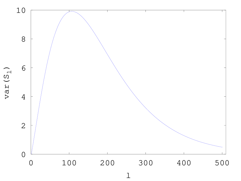
Figure 1:    Graph of $\text{var}(S_{l})$ for $n=100,k=20$

The case $c>1$ works the same way except that one uses the conditional distribution (2.6) rather than (2.3) in computing ${\mathbb{E}}[X_{l+1}^{q}|S_{l}]$, $q=1,2$; all of the equations (2.7), (2.9), (2.2) and (2.13) remain as before except that one generalizes the definitions of the coefficients $\{a_{i}\}$ (2.8) and $\{b_{i}\}$ (2.12) to

$$a_{0} \doteq c(n-k)/(n-1),~{}~{}~{}a_{1}\doteq(n-1-c)/(n-1),$$ (2.15)

$$b_{0} \doteq\frac{c((n-(c+1))+(n-k)(c-1))(n-k)}{(n-2)(n-1)},$$

$$b_{1} \doteq\frac{c(n-(c+1))(2(n-k)-1)}{(n-2)(n-1)},~{}~{}~{}b_{2}\doteq 1-\frac{2c}{n-1}+\frac{c(c-1)}{(n-1)(n-2)}.$$

Note that these reduce to (2.8) and (2.12) for $c=1.$ We summarize the formulas derived about the distribution of $Y(n,k)$ in Table 1.

	Distribution	Expectation	Second moment
$c=1$	(2.4), (2.5)	(2.10)	(2.14)
change for $c\geq 1$	(2.3)$\rightarrow$ (2.6)	(2.8) $\rightarrow$ (2.15)	(2.12) $\rightarrow$ (2.15)

Table 1: Equation numbers for the distribution and moments of $Y(n,k)$

3 A numerical comparison of push and pull

Let us now use the results so far to numerically compare the push and the pull algorithms. The observations made in this section will also motivate the theoretical results of the next chapter. As in subsection 2.1, let $I_{m}$ denote the number of infected nodes after the $m^{th}$ round. We have shown in that subsection how to write $I_{m}$ in terms of $S$. The Markov property of $S$ implies that one can also write the same sequence as

$$I_{m}=I_{m-1}+Y_{m},$$ (3.16)

where $Y_{m}$, conditioned on $I_{m-1}=j$, is independent of $(I_{0},I_{1},...,I_{m-2})$ and has the same distribution as $Y(n,j)$. One of the key questions about the process $(I_{0},I_{1},I_{2},...)$, and hence about the push algorithm is this: how many rounds is required so that a given proportion of the network is infected? This is the quantity that all of [19, 17, 21, 8] analyze. The answer to this question is expressed as the following stopping time of $I$:

$$\nu_{\lambda}^{n}\doteq\inf\{m:I_{m}/n\geq\lambda\},\lambda\in(0,1).$$ (3.17)

We compute the weak limit of $\nu^{n}_{\lambda}$ as the network size goes to $\infty$ in subsection 4.4. In the numerical study of the present section, we compute $N(\lambda,k)\doteq{\mathbb{E}}_{k}\left[\nu_{\lambda}^{n}\right]$, for $n=500$ and $c\in\{1,7\}$; the $k$ in the subscript of the expectation operator denotes that we condition on $I_{0}=k$, i.e., the infected number of nodes in the network before the first round is $k$. $N(1,k)$ is called the mean total dissemination time. Because $n$ is fixed (i.e., we are not taking any limits) throughout this section, there is no harm in assuming $\lambda\in\{j/n,0<j<n\}$, which is the set of all possible proportions of infected nodes for a finite network with $n$ nodes. The dynamics (3.16) implies that for $\lambda>k/n$

$$N(\lambda,k)=1+N(\lambda,k)\mathbb{P}(Y(n,k)=0)+\sum_{i=1}^{n\lambda-k-1}N(\lambda,k+i)\mathbb{P}(Y(n,k)=i).$$ (3.18)

The $1$ on the right means that going from $k$ infected nodes to $j=n\lambda$ infected nodes will take at least one round, the second term handles the case where no infections occur in the first round and the sum handles the cases where the first round infects at least $1$ node but less than the $j-k$ needed to get a total of $j$ infected nodes. Furthermore

$$N(\lambda,k)=0$$ (3.19)

when $\lambda\leq k/n$ because if there are $k$ infected nodes initially then obviously $j=\lambda n\leq k$ of them are also infected already and we need no rounds. (3.19), (3.18) and (2.5) can be used to compute $N(j/n,k)$ for all $j$ and $k$. Note that (3.18) and (3.19) are the same for the pull algorithm as well, the only change is in the distribution of $Y(n,k)$, which is binomial for the pull. Figure 2 shows $\lambda\rightarrow N(\lambda,k)$ for the push and the pull algorithms for $k=50$, $n=500$ and $c\in\{1,7\}$. These values of $k$ and $n$ correspond to $k/n=50/500=0.1$ initial proportion of infected nodes.

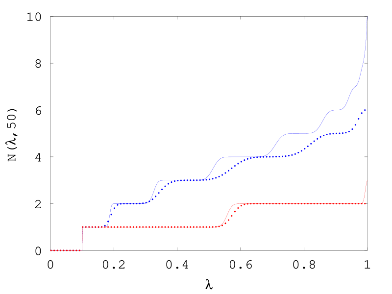
Figure 2:    Graphs of $\lambda\rightarrow N(\lambda,k)$ for the push and the pull algorithms; the dotted curves are pull, the solid curves are push; $n=500$, $k=50$, $c\in\{1,7\}$, the top couple is $c=1$ and the bottom couple is $c=7$

Figure 2 suggests that, for both push and pull, $\lambda\rightarrow N(\lambda,k)$ alternates between phases of constancy and rapid growth and that this behavior gets more marked as $c$ increases. One of the goals of the next section is to explain this behavior. For now, let us briefly comment that both of these algorithms have deterministic fluid limits (derived for the push algorithm in Theorem 1 and in subsection 4.3) and as the network size grows each round infects an almost deterministic proportion of the nodes. This can be used to prove that, in the limit, $\nu^{n}_{\lambda}$ becomes almost deterministic and as a function of $\lambda$ it becomes a step function, increasing only at the levels of infection attained by the rounds of the fluid limit; the exact result on this is Theorem 4, proved in subsection 4.4. The more pronounced nature of the growth phases for greater values of $c$ will again be explained by Theorem 1 which implies that the deviations from the fluid limit has a lower variance as $c$ grows.

The $N$ of the pull algorithm in Figure 2 lies on or below that of push. This suggests, for a large network with a nonzero initial proportion of infected nodes, on average, the pull reaches a given level in less or equal number of rounds than the push. However, note that the difference between the algorithms in Figure 2 is not that great and grows only as the network nears complete infection. The theoretical result which explains these observations is Proposition 1 in subsection 4.1, which compares the expected number of infected nodes in a pull and a push round.

[19, Section 6] uses the binomial distribution of $Y$ under the pull algorithm to compute the dependence on the fanout $c$ of the mean total dissemination time $N(1,1)$ starting with a single infected node for a network of $500$ nodes. With (2.5) we are able to do the same also for the push algorithm. $N(1,1)$ as a function of $c$ for $n=500$ is given in Figure 3 for both algorithms. Although $N(1,1)$ is larger in the push algorithm for smaller fanout values, this value for both algorithm seem to converge for $c\geq 8$. Corollary 1 below partially explains this phenomenon.

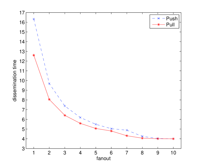
Figure 3:    Expected total dissemination time in rounds versus fanout for $n=500$, and $k=1$

4 Fluid and Diffusion Limits

A great deal can be understood about the push algorithm by computing the fluid and diffusion limits of $S$ as the network size $n$ goes to $\infty$. To get meaningful limits, we allow the initial number of infected nodes $k$ to depend on $n$ in such a way that

$$0<\mu=\lim_{n\rightarrow\infty}\frac{n-k_{n}}{n}<1$$ (4.20)

holds. The limits we talk of here are known as weak limits in probability theory and is almost always shown with the sign $\Rightarrow$, which we will also do below. The quintessential weak convergence result is the central limit theorem and “diffusion approximations” are central limit theorems for the entire sample paths of processes. Two of the basic references on weak convergence are [3, 11].

To get the fluid and diffusion limits, we scale and center $S$ and time as follows:

$$X^{n}_{t}\doteq\sqrt{n}\left(\frac{S_{\lfloor nt\rfloor}}{n}-\Gamma^{n}_{t}\right),~{}~{}~{}\Gamma^{n}_{t}\doteq\frac{\gamma_{\lfloor nt\rfloor}}{n}.$$ (4.21)

The time variable $t$ of the scaled processes $\Gamma^{n}$ and $X^{n}$ correspond to the $\lfloor nt\rfloor^{th}$ step of $S$; $\Gamma^{n}$ is the expected proportion of newly infected nodes at time $t$ and $X^{n}$ is $\sqrt{n}$ times the deviation of the actual proportion from the expected proportion, again at time $t$. This is the standard scaling in all diffusion analyses of Markovian random walks with finite variance increments. Just as in the central limit theorem, the scaling by $\sqrt{n}$ puts the difference between the actual and the expected proportions at a scale that ensures weak convergence to a nontrivial (i.e., neither $0$ nor $\infty$) limit.

The process $(X^{n},\Gamma^{n})$ takes values in $D_{{\mathbb{R}}^{2}}[0,\infty)$, the vector space of right continuous functions with left limits from $[0,\infty)$ to ${\mathbb{R}}^{2}$. Define

$$\Gamma_{t}\doteq(\Gamma_{0}-\mu)e^{-ct}+\mu,~{}~{}\sigma_{t}\doteq\sqrt{c(\mu-\Gamma_{t})(1-(\mu-\Gamma_{t}))}.$$ (4.22)

The next theorem gives the fluid and diffusion limits of $S$.

Theorem 1.

Let $(X^{n},\Gamma^{n})$ be defined as in (4.21) and $\Gamma$ as in (4.22). Let $X$ be given by

$$X_{t} \doteq X_{0}e^{-ct}+e^{-ct}\int_{0}^{t}e^{cs}\sigma_{s}dW_{s},$$ (4.23)

where $c\in\mathbb{Z}_{+}$ and $\sigma$ is as in (4.22). Then $(X^{n},\Gamma^{n})\Rightarrow(X,\Gamma).$

The proof, given in the appendix, is based on representing Markov processes and their weak convergence in terms of the semigroups that the processes define and the generators of these semigroups [11].

Theorem 1 implies that the random walk $\{S_{l}\}$ behaves more like
$\left\{n\left(\Gamma_{l/n}+\frac{1}{\sqrt{n}}X_{l/n}\right)\right\}$ as $n$, the network size, increases. The left part of Figure 4 shows $\{n\Gamma_{l/n}\}$ and a sample path of $\{S_{l}\}$ and its right part shows their difference. The random path of $S_{l}$ in this figure has been simulated using (2.3). Theorem 1 implies that the pathwise distribution of this difference gets closer to that of $\{\sqrt{n}X_{l/n}\}$ as $n$ increases.

Remember that $Y(n,k_{n})$ can be represented as the value $S_{k_{n}}$ of $S$ at step $k_{n}$, which corresponds to time $1-\mu$ in the scaled continuous time. Theorem 1 then implies in particular that $n\Gamma_{1-\mu}+\sqrt{n}X_{1-\mu}$ is the normal approximation of $Y(n,k_{n})$. Let us write this as

$$Y(n,k_{n})\approx n\Gamma_{1-\mu}+\sqrt{n}X_{1-\mu}.$$ (4.24)

The random variable on the right is normally distributed with mean $n\Gamma_{1-\mu}$. To compute its variance we only need the second moment of $X_{1-\mu}$, which we derive now. It will be simpler to write everything in terms of

$$\bar{X}_{t}\doteq\int_{0}^{t}e^{cs}\sigma_{s}dW_{s}.$$ (4.25)

The second moment of $X_{t}$ is

$$\text{var}(X_{t})\doteq e^{-2ct}{\mathbb{E}}[\bar{X}_{t}^{2}].$$ (4.26)

$\bar{X}_{t}$ is a stochastic integral with respect to a Brownian motion, and therefore $t\rightarrow\bar{X}_{t}$ is a continuous martingale whose quadratic variation equals [16, page 139]

$$\langle\bar{X}\rangle_{t} =\int_{0}^{t}e^{2cs}\sigma_{s}^{2}ds=\mu\left(e^{ct}-1-\mu ct\right),$$ (4.27)

which is a deterministic process. This implies ${\mathbb{E}}[\bar{X}_{t}^{2}]=\langle\bar{X}\rangle_{t}$ (see again [16, page 137]). This and setting $t=(1-\mu)$ in (4.26) gives

$$n\mu e^{-2c(1-\mu)}\left(e^{c(1-\mu)}-1-\mu(1-\mu)c\right)$$ (4.28)

as our approximation of the variance of $Y(n,k_{n}).$

                 

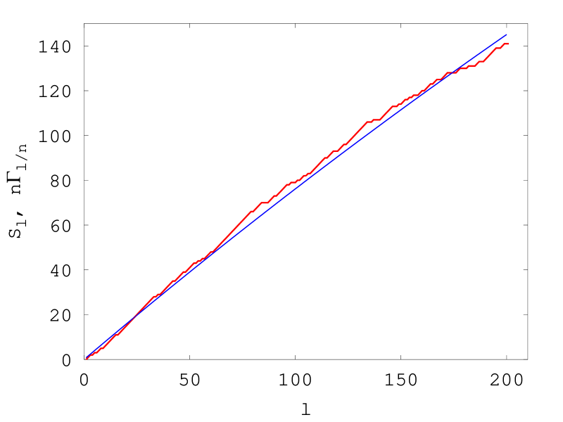
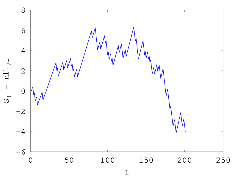
Figure 4: A sample path of $S_{l}$, $n\Gamma_{l/n}$ and their difference; $n=500$, $k_{n}=200$ and $c=1$

4.1 Comparison of push and pull for large networks

Theorem 1 allows a simple comparison of the push and the pull algorithms when $n$ is large. In this subsection it will be easier to use a separate symbol to denote the number of newly infected nodes in a pull round; let us use $\tilde{Y}(n,k)$ for this purpose. It is well known (see [19]) and simple to see that $\tilde{Y}(n,k)$ is Binomial$(1-p_{n},n-k)$ with failure probability $p_{n}=\binom{n-k-1}{c}/\binom{n-1}{c}$.

Proposition 1.

Let $\mu$ and $k_{n}$ be as in (4.20). Then ${\mathbb{E}}[\tilde{Y}(n,k_{n})]>{\mathbb{E}}[Y(n,k_{n})]$ for $n$ large.

Proof.

Theorem 1 says that the average proportion of newly infected nodes after a push round converges to $\Gamma_{1-\mu}=\mu(1-e^{-c(1-\mu)})$. The expected proportion of newly infected nodes in a pull round will be ${\mathbb{E}}[\tilde{Y}(n,k_{n})/n]=(1-p_{n})(n-k_{n})/n$, the mean of Binomial$(1-p_{n},n-k_{n})$ divided by $n$. Since $c$ is fixed, $p_{n}\rightarrow\mu^{c}.$ This and $(n-k_{n})/n\rightarrow\mu$ imply $\lim_{n}{\mathbb{E}}[\tilde{Y}(n,k_{n})/n]=\mu(1-\mu^{c}).$ The inequality

$$\mu(1-\mu^{c})>\mu\left(1-e^{-c(1-\mu)}\right)$$ (4.29)

for all $\mu$ and $c$ implies the statement of the proposition. ∎

Corollary 1.

For all $\mu$, if $c$ is taken large enough, a single round of pull or push is enough to infect the whole network.

Proof.

Both sides of (4.29) converge to $\mu$, the initial proportion of susceptible nodes as $c\rightarrow\infty$. ∎

Several comments on these results and possible research directions that they suggest are as follows. While the inequality (4.29) holds, the difference between the two sides is at most $0.06$ for $c=1$ and decreases as $c$ increases (simple calculus shows the truth of these statements). Thus, the performance of these rounds are on average similar, which explains the near performance of the pull and the push in the numerical example given in Figure 2.

There is an important caveat to Proposition 1, which we would like explain with an example. As with all values of $\mu$, for $\mu$ close to $1$, i.e., when initially most of the nodes are susceptible, a pull round infects on average more nodes than push, as indeed claimed by Proposition 1. But a push round takes merely $(1-\mu)n$ random selections whereas the pull takes $\mu n$; for large $\mu$, a push round is a very small operation whereas a pull round involves almost the whole network. Thus, for a fairer comparison we think that it would be a good idea to take into account the sizes of these operations. Such a comparison can be undertaken in future work.

An interesting comparison is when $\mu=0.5$ and the initial number of the infected nodes equal the number of the susceptible ones. In this case push and pull will involve the same number of random selections. For $c=1$, (4.29) implies that the pull round infects on average fifty percent of the susceptible nodes whereas the push approach infects around forty percent. For increasing values of $c$ the difference quickly disappears and for $c\geq 15$ a single round of either algorithm is enough to infect the whole network.

The foregoing discussion suggests the following heuristic: in a network with few infected nodes, initially set $c$ to a relatively high value (say between $10$ and $15$, if possible) use push until half the network is infected and then switch to pull and gradually decrease $c$. For smaller values of $c$, it will be more advantageous to switch to pull earlier. Obviously, to turn these ideas into a full fledged algorithm requires more work including a specification of how the nodes detect the infection level in the network to do the switch. The design of such an algorithm and its analysis can also be the subject of future work.

4.2 First time to hit $n\Gamma_{1-\mu}$

We have seen in the previous subsection that for $\mu=1/2$ and $c\geq 15$ one expects a single round to be enough to infect the whole network. In such cases, the number of rounds before the proportion of infected nodes hits a certain level becomes trivial (i.e. just $1$), and “the number of random selections” before the same event becomes more useful and interesting. (4.24) implies that, under (4.20), the ratio of the number of newly infected nodes to the number of nodes in the whole network at the end of the first round has expectation approximately $\Gamma_{1-\mu}$. The number of random selections needed to hit this level corresponds to the following stopping time of $S$: $\tau_{n}\doteq\inf\{l:S_{l}\geq n\Gamma_{1-\mu}\}$. The goal of this subsection is to derive approximations to the distribution of $\tau_{n}$ using the diffusion approximation of Theorem 1. The results we obtain will also be useful in subsection 4.4 in finding the limits of $\nu_{\lambda}^{n}$, the number of rounds needed before the infection level of the network is $\lambda.$ We would like to point out that $\tau_{n}$ cannot be studied if one represents the result of a push round as a single random variable, the ensuing analysis requires the use of the random walk representation.

Choose $t_{n}$ so that it solves

$$\Gamma_{1-\mu}-\Gamma_{t_{n}}=C\sqrt{\frac{\text{var}(X_{1-\mu})}{n}},$$ (4.30)

where $C>0$ is a large constant. (4.26) and (4.27) imply

$$t_{n}\doteq-\frac{1}{c}\log\left(\frac{1}{\mu}\left(\mu-\Gamma_{1-\mu}+\frac{C}{\sqrt{n}}\sqrt{\text{var}(X_{1-\mu})}\right)\right).$$ (4.31)

Taylor expanding $\log$ in the last display around $1-\Gamma_{1-\mu}/\mu$ gives

$$t_{n}=1-\mu-\frac{C\sqrt{\text{var}(X_{1-\mu})}}{c(\mu-\Gamma_{1-\mu})\sqrt{n}}+O(1/n).$$ (4.32)

Proposition 2.

$$\mathbb{P}(\tau_{n}\leq nt_{n})\leq\sqrt{\frac{2}{\pi}}\int_{C}^{\infty}e^{\frac{-x^{2}}{2}}dx,$$ (4.33)

for $n$ large enough.

We refer the reader to the appendix for the proof. Proposition 2 implies that, once we choose $C$ large enough, with very high probability $\tau_{n}>nt_{n}$ and, by (4.32), $nt_{n}$ is only $O(\sqrt{n})$ steps away from $n(1-\mu)=k_{n}.$ We will use this in the proof of the next theorem to focus our attention on a small neighborhood around $k_{n}$.

Theorem 2.

$(\tau_{n}-k_{n})/\sqrt{n}\Rightarrow N(0,v)$ where $v\doteq\text{var}(X_{1-\mu})/(c(\mu-\Gamma_{1-\mu}))^{2}.$

Proof.

Fix a finite interval $(a,b)$; our goal is to show

$$\lim_{n}\mathbb{P}\left(\frac{\tau_{n}-k_{n}}{\sqrt{n}}\in(a,b)\right)=\frac{1}{\sqrt{2\pi v}}\int_{a}^{b}e^{-x^{2}/2v}dx.$$ (4.34)

Choose $C$ in (4.30) so that

$$C>\frac{c(\mu-\Gamma_{1-\mu})}{\sqrt{\text{var}(X_{1-\mu})}}\max(|a|,|b|)$$

and define ${\bf t}_{n}\doteq k_{n}/n-t_{n}.$ Partition the event $E\doteq\{(\tau_{n}-n(1-\mu))/\sqrt{n}\in(a,b)\}$ as $(E\cap\{\tau_{n}<nt_{n}\})\cup(E\cap\{\tau_{n}\geq nt_{n}\}).$ Proposition 2 implies that, by increasing $C$, if necessary, the probability of the first of these sets can be made arbitrarily small. Furthermore, on the set $E$ the greatest value that $\tau_{n}$ can take is $k_{n}+b\sqrt{n}$; by the choice of $C$ this is bounded above by $k_{n}+n{\bf t}_{n}.$ These imply that we can replace $\tau_{n}=\inf\{l:S_{l}\geq n\Gamma_{1-\mu}\}$ in (4.34) with $\tau_{n}^{\prime}\doteq\inf\{l\in I_{n}:S_{l}\geq n\Gamma_{1-\mu}\}$, where $I_{n}\doteq k_{n}+n{\bf t}_{n}(-1,1)$. Thus in the rest of this argument we will prove

$$\lim_{n}\mathbb{P}\left(\frac{\tau_{n}^{\prime}-k_{n}}{\sqrt{n}}\in(a,b)\right)=\frac{1}{\sqrt{2\pi v}}\int_{a}^{b}e^{-x^{2}/2v}dx.$$ (4.35)

For this, it is enough to study the asymptotics of the dynamics of $S$ in the interval $I_{n}$. To do so, define the scaled process

$$\hat{X}^{n}_{\hat{t}}\doteq\frac{1}{\sqrt{n}}\left(S_{\lfloor k_{n}+\hat{t}\sqrt{n}\rfloor}-n\Gamma_{1-\mu}\right).$$

The scaled time $\hat{\tau}_{n}\doteq\frac{\tau_{n}^{\prime}-k_{n}}{\sqrt{n}}$ of (4.35) is the first time the process $\hat{X}^{n}$ hits $0$. Thus to find its limit distribution it is enough to compute the weak limit of $\hat{X}^{n}$, which we will now do.

The time interval $J_{n}\doteq[-\theta_{n},\theta_{n}]=\sqrt{n}{\bf t}_{n}[-1,1]$ for the process $\hat{X}^{n}$ corresponds exactly to the time interval $I_{n}$ for $S$ and therefore, we will be studying $\hat{X}^{n}$ on $J_{n}.$ Note that $t=0$ is the middle of $J_{n}$ and corresponds to time $k_{n}$ of $S$, which is the last step of the first push round. The end of $J_{n}$ is the time point $\theta_{n}=\sqrt{n}{\bf t}_{n}$. $k_{n}/n\rightarrow(1-\mu)$ and (4.32) imply

$$\theta_{n}\rightarrow\theta\doteq\frac{C\sqrt{\text{var}(X_{1-\mu})}}{c(\mu-\Gamma_{1-\mu})}.$$

$J_{n}=[-\theta_{n},\theta_{n}]$ is symmetric around $0$ and its starting point $-\theta_{n}$ converges to $-\theta.$ Then the limit process $\hat{X}$ of $\hat{X}^{n}$ will be running on the interval $[-\theta,\theta]$. Note that the initial point of $\hat{X}^{n}$ is $\hat{X}^{n}_{-\theta_{n}}=\frac{1}{\sqrt{n}}(S_{t_{n}}-n\Gamma_{1-\mu})$. Theorem 1, $t_{n}/n\rightarrow(1-\mu)$, and (4.30) imply that this random variable converges weakly to a normal random variable with mean $-C\sqrt{\text{var}(X_{1-\mu})}<0$ and variance $\text{var}(X_{1-\mu})$. Hence, this is the distribution of the limit $\hat{X}(-\theta).$

To compute the dynamics of $\hat{X}$ one proceeds parallel to the proof of Theorem 1. Fix $(\hat{x},\hat{t})\in{\mathbb{R}}\times[-\theta,\theta]$ and define

$$\hat{T}_{n}\doteq{\mathbb{E}}_{(\hat{x},\hat{t})}\left[f\left(\hat{X}^{n}_{\hat{t}+1/\sqrt{n}}\right)\right],\hat{A}_{n}\doteq\sqrt{n}(\hat{T}_{n}-I),$$

where $f$ is a smooth function on ${\mathbb{R}}$ with compact support. The subscript $(\hat{x},\hat{t})$ of the expectation means that we are conditioning of $\hat{X}^{n}_{t}=\hat{x}.$ It remains to compute $\hat{A}_{n}$. This computation is parallel to the arguments given in the proof of Theorem 1 with one important difference: now time is scaled by $1/\sqrt{n}$ rather than $1/n$. Thus, we omit the details and directly write down the limit: $\lim_{n\rightarrow\infty}A_{n}f=f^{\prime}(\hat{x})c(\mu-\Gamma_{1-\mu}).$ The right side of the last display is the generator of the process

$$\hat{X}_{\hat{t}}\doteq\hat{X}_{-\theta}+c(\mu-\Gamma_{1-\mu})(\hat{t}+\theta)$$ (4.36)

whose randomness is completely determined by its initial position $\hat{X}_{-\theta}$. Exactly the same line of arguments as in the proof of Theorem 1 now imply $\hat{X}^{n}\Rightarrow\hat{X}.$ We are interested in the limit of $\mathbb{P}(\hat{\tau}_{n}\in(a,b))$, the probability that $\hat{X}^{n}$ hits $0$ between time points $a$ and $b$. The weak limit we have just established implies that this limit equals $\mathbb{P}(\hat{\tau}\in(a,b))$ where $\hat{\tau}$ is the first time when the limit process $\hat{X}$ hits $0$. (4.36) implies that it will take $\hat{X}$ $\frac{-\hat{X}_{-\theta}}{c(\mu-\Gamma_{1-\mu})}$ unit of time to hit $0$. We subtract from this $\theta$ to convert it to the time unit of the limit time interval $[-\theta,\theta]$: $\tau^{\prime}=-\hat{X}_{-\theta}/c(\mu-\Gamma_{1-\mu})-\theta.$ But this is a random variable with mean $0$ and variance $v$. Hence we have (4.35).

∎

Here is a numerical example for Theorem 2. Suppose we have a network with $n=5000$ nodes of which $k=200$ are initially infected, i.e., $\mu=0.96$. Suppose that fanout is $c=5$. For this network, the $v$ that appears in Theorem 2 is $v\approx 0.0012$. We know from Theorem 1 that on average at the end of the first push round the total number of infected nodes will be $200+n\Gamma_{1-\mu}\approx 1070$. Now Theorem 2 says that the first push round will attain this infection level with probability approximately equal to $1/2$: and if it does, this will almost certainly happen in the last $4\sqrt{5000v}\approx 10$ steps of the push round (which lasts a total of $k=200$ steps); this network hitting $1070$ infected nodes before the last $10$ random selections is as likely as a normal random variable being $4$ standard deviations below its mean. The same theorem implies that with probability $1/2$ this level will be attained approximately in the first $10$ steps of the next round.

For $0<\lambda<\mu$, define $\tau^{n}_{\lambda}\doteq\inf\{l:S_{l}\geq n\lambda\}.$ $\tau^{n}_{\lambda}$ is the number of random selections before the proportion of newly infected nodes has reached $\lambda$; in terms of the random walk $S$, it is the first time $S$ reaches the level $n\lambda.$

Define

$$\bar{\tau}_{\lambda}(\mu)\doteq-\frac{1}{c}\log\left(1-\frac{\lambda}{\mu}\right)$$ (4.37)

$\bar{\tau}$, as a function of $\lambda$, is the inverse function of the fluid limit $\Gamma_{t}(\mu)=\mu(1-e^{-ct})$ with respect to $t$. Dynamically, $\bar{\tau}_{\lambda}$ is the first time $\Gamma$ hits the level $\lambda.$ Because $\Gamma$ is deterministic, so is this hitting time. A quick examination of the proof of Theorem 2 reveals that if one replaces $1-\mu$ with $\bar{\tau}_{\lambda}$ and $\Gamma_{1-\mu}$ with $\lambda$, the proof continues to work exactly as is. This gives us the following generalization of Theorem 2:

Theorem 3.

Let $\tau^{n}_{\lambda}$ and $\bar{\tau}_{\lambda}$ be as above. $(\tau^{n}_{\lambda}-n\bar{\tau}_{\lambda})/\sqrt{n}\Rightarrow N(0,v)$ with $v=\text{var}(X_{\bar{\tau}_{\lambda}})/(c(\mu-\lambda))^{2}.$

4.3 Fluid limit of the whole push algorithm

As suggested in the beginning of this section, instead of the number of newly infected nodes, one can keep track of their proportion in the network. This amounts to dividing $S$ by $n$. Theorem 1 gives us the following approximation for the proportion process: $S_{l}/n\approx\Gamma_{l/n}+\frac{1}{\sqrt{n}}X_{l/n}$ Thus as $n$ goes to infinity, the proportion process $S/n$ converges to its fluid limit $\Gamma$. In subsection 2.1 we have argued that the random walk $S$, when ran indefinitely, is a model for the whole push algorithm. This implies that $t\rightarrow\Gamma_{t}$ for $t\in(0,\infty)$ is a representation of the fluid limit of the whole push algorithm. To break it into rounds, we proceed as follows. Define $\varphi_{0}\doteq(1-\mu)$, this is the initial proportion of infected nodes in the fluid limit. The first round in the prelimit lasts $k_{n}$ steps; in the scaled limit time, this corresponds to the time point $\lim_{n}k_{n}/n=1-\mu$, thus the first round of the fluid limit ends at time $1-\mu$ and the total proportion of infected nodes after the first round is $\varphi_{1}\doteq\varphi_{0}+\Gamma_{\varphi_{0}}$. The next fluid round will last a time interval of length $\varphi_{1}$ and will add an additional $\Gamma_{\varphi_{0}+\varphi_{1}}-\Gamma_{\varphi_{0}}$ proportion of infected nodes, bringing the total proportion of infected nodes at the end of the second round to $\varphi_{2}\doteq\varphi_{0}+\Gamma_{\varphi_{1}+\varphi_{0}}$ In general, the proportion of infected nodes at the end of the $i^{th}$ round of the fluid limit will be

$$\varphi_{i}=\varphi_{0}+\Gamma_{c_{i-1}},$$ (4.38)

with $c_{i-1}\doteq\sum_{j=0}^{i-1}\varphi_{j}$. The construction of $\{\varphi_{0},\varphi_{1},\varphi_{2},...\}$ is the fluid limit version of that of the sequence $(I_{0},I_{1},I_{2},...)$ given in subsection 2.1; and indeed, Theorem 1 implies $I_{i}/n\Rightarrow\varphi_{i}.$ The sequence $\{\varphi_{i}\}$ is increasing and deterministic; in the fluid limit, each round infects a deterministic proportion of the network. In the next subsection we will use the sequence $\{\varphi_{i}\}$ to compute the weak limit of $\nu^{n}_{\lambda}$, the number of push rounds in a network with $n$ nodes before the proportion of the infected nodes in the network hits $\lambda$.

4.4 Weak limit of $\nu_{\lambda}^{n}$

Recall that $\nu_{\lambda}^{n}$, defined in (3.17), is the number of push rounds needed before the proportion of the infected nodes in the network reaches $\lambda\in(0,1)$. Section 3 presents numerical computations of the expectation of this random variable for a network with $500$ nodes and for different fanout values and makes several observations about the results. Here, we derive the weak limit of this random variable using the sequence $\{\varphi_{i}\}$ of (4.38) and Theorems 1 and 3.

Define $\bar{\nu}_{\lambda}\doteq\inf\{i:\varphi_{i}\geq\lambda\};$ $\bar{\nu}$ is the number of rounds that the fluid limit network needs so that its proportion of infected nodes equals $\lambda$. Because $\varphi$ is an increasing deterministic sequence, $\bar{\nu}_{\lambda}$ can be characterized as follows: $\bar{\nu}_{\lambda}=i$ for $\lambda\in[\varphi_{i},\varphi_{i+1})$. Hence, as function of $\lambda$, $\bar{\nu}$ is right continuous, piecewise constant and it jumps precisely by $1$ at the points $\{\varphi_{1},\varphi_{2},\varphi_{3},...\}.$ As the final step of our analysis of the push algorithm we prove

Theorem 4.

$\nu_{\lambda}^{n}\Rightarrow\bar{\nu}_{\lambda}$ for $\lambda\in(0,1)-\{\varphi_{0},\varphi_{1},\varphi_{2},...\}$.

Proof.

$\nu_{\lambda}=\bar{\nu}_{\lambda}=0$ for $\lambda\leq\varphi_{0}=1-\mu$; i.e., if $\lambda$ is less than $1-\mu$ (the initial proportion of infected nodes), the network already has more than $\lambda$ proportion of infected nodes before any round begins.

To keep the proof short, we will treat the first two rounds; an argument that covers all rounds will involve the same ideas. Fix a $\lambda\in(\varphi_{0},\varphi_{1})$; we would like to show that $\nu_{\alpha}^{n}\Rightarrow\bar{\nu}_{\lambda}=1$, i.e., as $n$ goes to $\infty$, the infection level $\lambda$ is attained in the first round with probability approaching $1$. $\lambda<\varphi_{1}$, and the definitions (4.38) and (4.37) of $\varphi_{1}$ and $\bar{\tau}_{\lambda}$ imply

$$\bar{\tau}_{\lambda}<1-\mu;$$ (4.39)

this last inequality can also be expressed as follows: at time $1-\mu$ the proportion of infected nodes in the fluid limit is $\varphi_{1}$; $\lambda$ being strictly less than $\varphi_{1}$ and the fluid limit $\Gamma$ being strictly increasing and deterministic, it must be that the first time the fluid limit has reached the infection level $\lambda$ must be before time $1-\mu$.

$\nu_{\alpha}^{n}=1$ if and only if $\tau^{n}_{\lambda}\leq k_{n}$, which is the same inequality as

$$\frac{1}{\sqrt{n}}\left(\frac{1}{\sqrt{n}}\left(\tau^{n}_{\lambda}-n\bar{\tau}_{\lambda}\right)\right)\leq k_{n}/n-\bar{\tau}_{\lambda}.$$ (4.40)

The first term on the left is a constant and converges to $0$; Theorem 3 says that the second term on the left converges weakly to a finite random variable. Thus, their product converges weakly to $0$. (4.39) and $k_{n}/n\rightarrow(1-\mu)$ imply, on the other hand, that the limit of the right side is strictly greater than $0$. Thus, the probability of the event expressed in this display, that is, the probability that $\nu_{\lambda}=1$, indeed converges to $1$.

For $\lambda\in(\varphi_{1},\varphi_{2})$, we would like to show $\nu_{\lambda}^{n}$ converges weakly to $\bar{\nu}_{\lambda}=2$, i.e., we want to show that the probability of the event $k_{n}<\tau_{\lambda}<k_{n}+S_{k_{n}}$ converges to $1$ ($k_{n}$ is the total number of random selections in the first round and $k_{n}+S_{k_{n}}$ is the same total after the second round). A rescaling and centering similar to (4.40) and Theorems 1, 3 imply this. ∎

An interesting question is the weak limit of $\nu_{\varphi_{i}}^{n}$. We have already covered the case $i=1$ in the argument given in the numerical example following Theorem 2: $\nu_{\varphi_{1}}^{n}\Rightarrow T_{1}$ where $T_{1}\in\{1,2\}$ and takes these value with equal probability. The weak limit of the whole sequence $\left\{\nu_{\varphi_{i}}^{n},i=1,2,3,...\right\}$ requires a longer analysis and we leave it to future work.

Figure 5 shows two graphs: first is that of $\bar{\nu}_{\lambda}$ for an initial infection rate of $\mu=0.01$ and fanout $c=3$; the second is $N(\lambda,5=500\mu)={\mathbb{E}}_{5}[\nu^{(500)}_{\lambda}]$; the graph of $N(\lambda,50)$ for $c\in\{1,7\}$ has been given earlier in Figure 2.

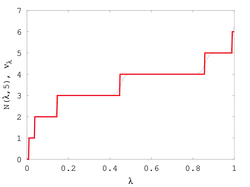
Figure 5:    The graphs of $\bar{\nu}_{\lambda}$ (the thicker curve) and $N(\lambda,5)$; both for $c=3$

Clearly, as Theorem 4 implies, these graphs overlap except around $\{\varphi_{i}\}$; at $\varphi_{i}$, $\bar{\nu}$ jumps by $1$ while $N$ rapidly goes from $i-1$ to $i$. Theorem 4 also implies that the $\lambda$ interval over which this transition occurs shrinks to the single point $\varphi_{i}$ as the network size grows to $\infty.$

5 Conclusion

The starting point of the analysis of the present paper is taking the random selections in a push round as the atomic operation of the push algorithm and defining a random walk whose each step corresponds to a random selection. The main body of the analysis consists of computing weak limits of this random walk and its various functions. We expect these ideas to be directly applicable to other epidemic algorithms (such as those considered in [17, 21]) over fully connected networks.

Fully connectedness is one of the natural limits of the collection of possible topologies over a given collection of nodes. As the topology of a network approaches full connectivity one expects the results for the latter to be good approximations for the former. One can further use results on quantities in fully connected networks as upper and lower bounds on the same quantities in other network topologies. After a detailed analysis of this basic case, an interesting and important direction is the generalization to more complex network topologies and structures, such as those considered in [8, 13, 2].

To the best of our understanding, most of the literature on the asymptotic analysis of epidemic algorithms focus on obtaining upperbounds on the tail probabilities of the total dissemination time, $\nu_{1}^{n}$ in our notation. For this, authors often use large deviations results such as Chernoff’s bound. However, the underlying processes in these models may have fluid and diffusion limits and these limits can give more precise information about the distribution of key random variables, such as the total dissemination time. We hope that the present work provides an example of how this path can be followed in the context of a simple model.

Appendix A Proofs

Proof of Theorem 1.

To avoid confusion between discrete and continuous time parameters, we will show continuous time parameters in parentheses, e.g., we will write $X^{n}(t)$ instead of $X^{n}_{t}.$ We begin by assuming that $c=1$, the modifications for $c>1$ will be straightforward. $k_{n}$ is assumed to grow with $n$ so that $\lim_{n}(n-k_{n})/n=\mu\in(0,1)$. Let $C_{b}({\mathbb{R}}^{2})$ denote the set of bounded and continuous functions on ${\mathbb{R}}^{2}$; and $C^{2}_{0}({\mathbb{R}}^{2})$ the set of twice differentiable functions with compact support with continuous Hessians. Define $T_{n}:C_{b}({\mathbb{R}}^{2})\rightarrow C_{b}({\mathbb{R}}^{2})$ as

$$[T_{n}(f)](x)={\mathbb{E}}_{x}[f(X^{n}(1/n),\Gamma^{n}(1/n))],x\in{\mathbb{R}}^{2},$$ (A.41)

where the subscript $x$ of ${\mathbb{E}}_{x}$ denotes conditioning on $(X^{n}(0),\Gamma^{n}(0))=x=(x_{1},x_{2}).$

Define

$$A_{n}\doteq n(T_{n}-I),$$ (A.42)

where $I$ denotes the identity operator on $C_{b}({\mathbb{R}}^{2}).$ Let us compute $A_{n}$ explicitly for $f\in C^{2}_{0}({\mathbb{R}}^{2})$. The expectation in (A.41) is conditioned on
$(X^{n}(0),\Gamma^{n}(0))=(x_{1},x_{2})$, i.e., on

$$\frac{S_{0}-\gamma_{0}}{\sqrt{n}}=x_{1},\frac{\gamma_{0}}{n}=x_{2}.$$ (A.43)

This, (2.2), (2.7) and the definition of $X^{n}$ imply

$$X^{n}(1/n)=\frac{S_{1}-\gamma_{1}}{\sqrt{n}} =\frac{S_{0}-\gamma_{0}}{\sqrt{n}}+\frac{S_{1}-S_{0}}{\sqrt{n}}-\frac{\gamma_{1}-\gamma_{0}}{\sqrt{n}}$$

$$=x_{1}+\left(X_{1}-\left(\frac{n-k_{n}}{n-1}-\frac{n}{n-1}x_{2}\right)\right)/\sqrt{n}$$

$$\Gamma^{n}(1/n) =\frac{\gamma_{1}}{n}=\frac{1}{n}\left(\gamma_{0}\frac{n-2}{n-1}+\frac{n-k_{n}}{n-1}\right)$$

$$=x_{2}-\frac{x_{2}}{n-1}+\frac{n-k_{n}}{n(n-1)}.$$

Define

$$Y_{1} \doteq X_{1}-\left(\frac{n-k_{n}}{n-1}-\frac{n}{n-1}x_{2}\right),$$ (A.44)

$$y_{2} \doteq-\frac{x_{2}}{n-1}+\frac{n-k_{n}}{n(n-1)},~{}~{}~{}\Delta\doteq(Y_{1}/\sqrt{n},y_{2})$$

where $X_{1}$ refers to the random variable given in (2.3). ${\mathbb{E}}_{x}[Y_{1}]$ and $E_{x}[Y_{1}^{2}]$ will be useful in what follows, so let us compute them first. Equations (A.43) and (2.3) give

$${\mathbb{E}}_{x}[X_{1}]=\frac{n-k_{n}}{n-1}-\frac{n}{n-1}x_{2}-\frac{\sqrt{n}}{n-1}x_{1},$$ (A.45)

which gives

$${\mathbb{E}}_{x}[Y_{1}]={\mathbb{E}}_{x}[X_{1}]-\left(\frac{n-k_{n}}{n-1}-\frac{n}{n-1}x_{2}\right)=-\frac{\sqrt{n}}{n-1}x_{1}.$$ (A.46)

On the other hand ${\mathbb{E}}_{x}[X_{1}]={\mathbb{E}}_{x}[X_{1}^{2}]=(n-k_{n}-nx_{2})/(n-1)$ implies

$${\mathbb{E}}_{x}[Y_{1}^{2}] ={\mathbb{E}}_{x}[X_{1}^{2}]+2{\mathbb{E}}_{x}[Y_{1}]d_{n}-d_{n}^{2}$$ (A.47)

$$=(n-k_{n}-nx_{2})/(n-1)-\frac{\sqrt{n}}{n-1}x_{1}d_{n}-d_{n}^{2}$$

where $d_{n}$ refers to the constant $(-(n-k_{n})+nx_{2})/(n-1)$ in $Y_{1}$’s definition.

The expectation that occurs in the definition (A.41) of $T_{n}$ written in terms of the vector $\Delta$ is ${\mathbb{E}}_{x}[f(X^{n}(1/n),\Gamma^{n}(1/n))]={\mathbb{E}}_{x}[f(x+\Delta)].$ Let $Df$ denote the gradient of $c$ and $Hf$ its Hessian; and let $\Delta^{2}$ denote the tensor product $\Delta\otimes\Delta.$ Using $f$’s Taylor’s expansion in the last display gives

$${\mathbb{E}}_{x}[f(X^{n}(1/n),\Gamma^{n}(1/n))]={\mathbb{E}}_{x}\left[f(x)+\langle Df(x),\Delta\rangle+\frac{1}{2}\langle Hf(x+\theta_{n}),\Delta^{2}\rangle\right]$$ (A.48)

where $\theta_{n}$ is a random vector that lies on the line segment connecting $0$ to $\Delta.$ Let us deal with each of the terms that appear in (A.48) one by one. The function $f(x)$ is not random and so it comes out of the expectation. The first order term is $\langle Df(x),\Delta\rangle=f_{x_{1}}(x)Y_{1}/\sqrt{n}+f_{x_{2}}(x)\,y_{2}.$ That the second term is deterministic and (A.46) give

$${\mathbb{E}}_{x}\left[\langle Df(x),\Delta\rangle\right]=-f_{x_{1}}(x)\frac{x_{1}}{n-1}+f_{x_{2}}(x)\,y_{2}.$$ (A.49)

${\mathbb{E}}_{x}\left[\langle Hf(\theta_{n}),\Delta^{2}\rangle\right]$ is

$$\frac{1}{n}{\mathbb{E}}_{x}\left[f_{x_{1},x_{1}}(x+\theta_{n})Y_{1}^{2}\right]+2y_{2}\frac{1}{\sqrt{n}}{\mathbb{E}}_{x}\left[f_{x_{1},x_{2}}(x+\theta_{n})Y_{1}\right]$$

$$~{}~{}~{}+(y_{2})^{2}f_{x_{2},x_{2}}(x+\theta_{n}).$$

Substituting these in (A.42) yields

$$A_{n}f =-f_{x_{1}}\frac{n}{n-1}x_{1}+f_{x_{2}}(x)(ny_{2})+\frac{1}{2}{\mathbb{E}}_{x}\left[f_{x_{1},x_{1}}(x+\theta_{n})Y_{1}^{2}\right]$$ (A.50)

$$~{}~{}~{}+y_{2}\sqrt{n}{\mathbb{E}}_{x}\left[f_{x_{1},x_{2}}(x+\theta_{n})Y_{1}\right]+\frac{1}{2}n(y_{2})^{2}f_{x_{2},x_{2}}(x+\theta_{n})$$

Now let us compute the limits of each of the terms in the last sum as $n\rightarrow\infty$. The first term converges to $-f_{x_{1}}x_{1}$. The definition of $y_{2}$ and (4.20) imply

$$\lim_{n\rightarrow\infty}f_{x_{2}}(x)(ny_{2})=f_{x_{2}}(\mu-x_{2}).$$ (A.51)

Note that

$$\theta_{n}\rightarrow 0$$ (A.52)

uniformly, because $\Delta$ is bounded. This and the continuity of $Hf$ imply

$$\lim_{n\rightarrow\infty}\frac{1}{2}{\mathbb{E}}_{x}\left[f_{x_{1},x_{1}}(x+\theta_{n})Y_{1}^{2}\right]=\frac{1}{2}f_{x_{1},x_{1}}(x)\lim_{n\rightarrow\infty}{\mathbb{E}}_{x}\left[Y_{1}^{2}\right].$$ (A.53)

The observation (A.52), continuity of $Hf$ and $|(y_{2})^{2}|=O(1/n^{2})$ imply

$$\lim_{n\rightarrow 0}\frac{1}{2}n(y_{2})^{2}f_{x_{2},x_{2}}(x+\theta_{n})=0.$$ (A.54)

Boundedness of $Y_{1}$, (A.46), (A.52), continuity of $Hf$ an $|y_{2}|=O(1/n)$ imply

$$\lim_{n\rightarrow\infty}y_{2}\sqrt{n}{\mathbb{E}}_{x}\left[f_{x_{1},x_{2}}(x+\theta_{n})Y_{1}\right]=0.$$ (A.55)

Letting $n\rightarrow\infty$ in (A.47) gives

$$\lim_{n\rightarrow\infty}{\mathbb{E}}_{x}\left[Y_{1}^{2}\right]=(\mu-x_{2})(1-(\mu-x_{2})).$$ (A.56)

The equations (A.50), along with (A.51), (A.53), (A.54), (A.55) and (A.56) yield $\lim_{n\rightarrow\infty}A_{n}f=Af$ where $Af\doteq\langle Df,(-x_{1},\mu-x_{2})\rangle+\frac{1}{2}(\mu-x_{2})(1-(\mu-x_{2}))f_{x_{1},x_{1}}.$ One can check directly that $A$ is the infinitesimal generator of the semigroup $T(\cdot)$ defined by the process $(X_{t},\Gamma_{t})$. It follows from its definition that $T(\cdot)$ is a Feller semigroup on $C_{b}({\mathbb{R}}^{2})$. Furthermore, [11, Proposition 3.2, page 17] imply that $C^{\infty}({\mathbb{R}}^{2})$ forms a core for the generator $A$. Thus, [11, Theorem 1.2, page 31] and [11, Theorem 2.6, page 168] imply $(X^{n},\Gamma^{n})\Rightarrow(X,\Gamma)$.

Modifications for $c>1$ are as follows. The variables $Y_{1}$ and $y_{2}$ are now defined as

$$Y_{1}\doteq X_{1}-c\,\left(\frac{n-k_{n}}{n-1}-\frac{n}{n-1}x_{2}\right),\qquad y_{2}\doteq-\frac{x_{2}\,c}{n-1}+\frac{(n-k_{n})\,c}{n(n-1)};$$

where $X_{1}$ has the hypergeometric distribution (2.6). Then

$$\mathbb{E}_{x}[Y_{1}]=-c\,\frac{\sqrt{n}}{n-1}x_{1}.$$ (A.57)

(A.47) becomes ${\mathbb{E}}_{x}[Y_{1}^{2}]={\mathbb{E}}_{x}[X_{1}^{2}]+2{\mathbb{E}}_{x}[Y_{1}]d_{n}-d_{n}^{2}={\mathbb{E}}_{x}[X_{1}^{2}]-\frac{c\sqrt{n}}{n-1}x_{1}d_{n}-d_{n}^{2}$ where $d_{n}$ is now $c(-(n-k_{n})+nx_{2})/(n-1)$. For the asymptotic analysis, we only need the limit of the last display as $n\rightarrow\infty.$ For $n$ large, one can approximate the hypergeometric $X_{1}$ as Binomial$(p^{*},c)$ with success probability $p^{*}=(k_{n}-nx_{2})/n$, whose second moment is $cp^{*}+c(c-1)(p^{*})^{2}.$ Substituting this in the last display and letting $n\rightarrow\infty$ we get

$$\lim_{n\rightarrow\infty}\mathbb{E}_{x}[Y_{1}^{2}]=c\,(\mu-x_{2})(1-(\mu-x_{2}))$$ (A.58)

which generalizes (A.56) to $c>1.$ On the other hand, we have
${\mathbb{E}}_{x}\left[\langle Df(x),\Delta\rangle\right]=-f_{x_{1}}(x)\,c\,\frac{x_{1}}{n-1}+f_{x_{2}}(x)\,y_{2}$ (generalization of (A.49)). It follows that

$$A_{n}f =-f_{x_{1}}\,c\,\frac{n}{n-1}x_{1}+f_{x_{2}}(x)(ny_{2})+\frac{1}{2}{\mathbb{E}}_{x}\left[f_{x_{1},x_{1}}(x+\theta_{n})Y_{1}^{2}\right]$$

$$~{}~{}~{}+y_{2}\sqrt{n}{\mathbb{E}}_{x}\left[f_{x_{1},x_{2}}(x+\theta_{n})Y_{1}\right]+\frac{1}{2}n(y_{2})^{2}f_{x_{2},x_{2}}(x+\theta_{n}).$$

Same arguments as in the $c=1$ case give $\lim_{n\rightarrow\infty}f_{x_{2}}(x)(ny_{2})=f_{x_{2}}\,c\,(\mu-x_{2}).$ The last two displays (A.57) and (A.58) imply $\lim_{n\rightarrow\infty}A_{n}f=Af$ where $Af\doteq\langle Df,c\,(-x_{1},\mu-x_{2})\rangle+\frac{1}{2}\,c\,(\mu-x_{2})(1-(\mu-x_{2}))f_{x_{1},x_{1}}.$ The rest of the proof is the same as in the case of $c=1.$ ∎

Proof of Proposition 2.

Define the stopping time

$$\tau_{n}^{\prime}\doteq\inf\left\{l:\frac{1}{\sqrt{n}}(S_{l}-\gamma_{l})\geq\frac{n\Gamma_{1-\mu}-\gamma_{\lfloor nt_{n}\rfloor}}{\sqrt{n}}\right\}.$$

$S_{l}\geq n\Gamma_{1-\mu}$ is the same as $(S_{l}-\gamma_{l})/\sqrt{n}\geq(n\Gamma_{1-\mu}-\gamma_{l})/\sqrt{n}$. That $\gamma_{l}$ is increasing in $l$ implies that the right side of this inequality is decreasing in $l$. This implies

$$\{\tau_{n}\leq nt_{n}\}\subset\{\tau_{n}^{\prime}\leq nt_{n}\}.$$ (A.59)

We know from Theorem 1 that $\gamma_{\lfloor nt_{n}\rfloor}/n\rightarrow\Gamma_{t}.$ This and (4.30) imply $\lim_{n}(n\Gamma_{1-\mu}-\gamma_{\lfloor nt_{n}\rfloor})/{\sqrt{n}}$ $\rightarrow$ $C\sqrt{\text{var}(X_{1-\mu})}$. Now define $\tau^{\prime}\doteq\inf$ $\{t:\bar{X}_{t}\geq C\sqrt{\text{var}(\bar{X}_{1-\mu})}\}.$ The last two displays, that $t\rightarrow e^{ct}$ is monotone increasing, $t_{n}\rightarrow(1-\mu)$ (see (4.32)) and Theorem 1 imply $\lim_{n\rightarrow\infty}\mathbb{P}(\{\tau_{n}^{\prime}\leq nt_{n}\})$ $\leq$ $\mathbb{P}(\tau^{\prime}\leq(1-\mu)).$ $\bar{X}$ is a stochastic integral against a Brownian motion. Therefore, if we measure time using its quadratic variation it will be a standard Brownian motion [16, Theorem 4.6, page 174]. This and [16, Equation (6.3), page 80] give $\mathbb{P}(\tau^{\prime}\leq(1-\mu))=\sqrt{\frac{2}{\pi}}\int_{C}^{\infty}e^{\frac{-x^{2}}{2}}dx.$ The last equality and (A.59) imply (4.33). ∎

References

- [1] Mert Akdere, Cemal Çagatay Bilgin, Ozan Gerdaneri, Ibrahim Korpeoglu, Özgür Ulusoy, and Ugur Cetintemel. A comparison of epidemic algorithms in wireless sensor networks. Computer Communications, 29(13):2450–2457, 2006.
- [2] Christos Anagnostopoulos, Stathes Hadjiefthymiades, and Evangelos Zervas. Information dissemination between mobile nodes for collaborative context awareness. Mobile Computing, IEEE Transactions on, 10(12):1710–1725, 2011.
- [3] Patrick Billingsley. Convergence of Probability Measures, Second Edition. Wiley, 1999.
- [4] Alexander Birman. Computing approximate blocking probabilities for a class of all-optical networks. Selected Areas in Communications, IEEE Journal on, 14(5):852–857, 1996.
- [5] Kenneth P. Birman, Mark Hayden, Oznur Ozkasap, Zhen Xiao, Mihai Budiu, and Yaron Minsky. Bimodal multicast. ACM Transactions on Computer Systems (TOCS), 17(2):41–88, 1999.
- [6] Béla Bollobás, Oliver Riordan, Joel Spencer, and Gábor Tusnády. The degree sequence of a scale-free random graph process. Random Structures & Algorithms, 18(3):279–290, 2001.
- [7] Tom Britton. Stochastic epidemic models: a survey. Mathematical biosciences, 225(1):24–35, 2010.
- [8] Flavio Chierichetti, Silvio Lattanzi, and Alessandro Panconesi. Rumor spreading in social networks. Theoretical Computer Science, 412(24):2602–2610, 2011.
- [9] Edward G. Coffman Jr, Zihui Ge, Vishal Misra, and Don Towsley. Network resilience: exploring cascading failures within bgp. In Proc. 40th Annual Allerton Conference on Communications, Computing and Control, 2002.
- [10] Daryl J. Daley and Joseph Mark Gani. Epidemic modelling: an introduction, volume 15. Cambridge University Press, 2001.
- [11] Stewart Ethier and Thomas G. Kurtz. Markov processes. characterization and convergence. NY: John Willey and Sons, 9, 1986.
- [12] Patrick T. Eugster, Rachid Guerraoui, Anne-Marie Kermarrec, and Laurent Massoulié. Epidemic information dissemination in distributed systems. Computer, 37(5):60–67, 2004.
- [13] Ayalvadi Ganesh, Laurent Massoulié, and Don Towsley. The effect of network topology on the spread of epidemics. In INFOCOM 2005. 24th Annual Joint Conference of the IEEE Computer and Communications Societies. Proceedings IEEE, volume 2, pages 1455–1466. IEEE, 2005.
- [14] Joe Gani. Random-allocation and urn models. Journal of Applied Probability, 41:313–320, 2004.
- [15] Richard Gibbens and Frank P. Kelly. Dynamic routing in fully connected networks. IMA Journal of Mathematical Control and Information, 7(1):77–111, 1990.
- [16] Ioannis Karatzas and Steven Eugene Shreve. Brownian motion and stochastic calculus, volume 113. Springer, 1991.
- [17] Richard Karp, Christian Schindelhauer, Scott Shenker, and Berthold Vocking. Randomized rumor spreading. In Foundations of Computer Science, 2000. Proceedings. 41st Annual Symposium on, pages 565–574. IEEE, 2000.
- [18] Jochen Mundinger, Richard Weber, and Gideon Weiss. Optimal scheduling of peer-to-peer file dissemination. Journal of Scheduling, 11(2):105–120, 2008.
- [19] Öznur Özkasap, Mine Çağlar, Şule Yazıcı, and Selda Küçükçifçi. An analytical framework for self-organizing peer-to-peer anti-entropy algorithms. Performance Evaluation, 67(3):141–159, 2010.
- [20] Dongyu Qiu and Rayadurgam Srikant. Modeling and performance analysis of bittorrent-like peer-to-peer networks. ACM SIGCOMM Computer Communication Review, 34(4):367–378, 2004.
- [21] Sujay Sanghavi, Bruce Hajek, and Laurent Massoulié. Gossiping with multiple messages. Information Theory, IEEE Transactions on, 53(12):4640–4654, 2007.
- [22] Henry C. Tuckwell and Ruth J. Williams. Some properties of a simple stochastic epidemic model of sir type. Mathematical biosciences, 208(1):76–97, 2007.
- [23] Di Warren and Eugene Seneta. Peaks and eulerian numbers in a random sequence. Journal of applied probability, pages 101–114, 1996.
- [24] Max A. Woodbury. On a probability distribution. The Annals of Mathematical Statistics, 20(2):311–313, 1949.
- [25] Shouhuai Xu, Wenlian Lu, and Li Xu. Push-and pull-based epidemic spreading in networks: Thresholds and deeper insights. ACM Transactions on Autonomous and Adaptive Systems (TAAS), 7(3):32, 2012.