Relativistic Coulomb excitation within Time Dependent Superfluid Local Density Approximation

Abstract

Within the framework of the unrestricted time-dependent density functional theory, we present for the first time an analysis of the relativistic Coulomb excitation of the heavy deformed open shell nucleus ²³⁸U. The approach is based on Superfluid Local Density Approximation (SLDA) formulated on a spatial lattice that can take into account coupling to the continuum, enabling self-consistent studies of superfluid dynamics of any nuclear shape. We have computed the energy deposited in the target nucleus as a function of the impact parameter, finding it to be significantly larger than the estimate using the Goldhaber-Teller model. The isovector giant dipole resonance, the dipole pygmy resonance and giant quadrupole modes were excited during the process. The one body dissipation of collective dipole modes is shown to lead a damping width $\Gamma_{\downarrow}\approx 0.4$ MeV and the number of pre-equilibrium neutrons emitted has been quantified.

Coulomb excitation represents an ideal method to probe the properties of large amplitude nuclear motion, because the excitation process is not obscured by uncertainties related to nuclear forces. The excitation probabilities are governed by the strength of the Coulomb field only and they can be fully expressed in terms of the electromagnetic multipole matrix elements Winther and Alder (1979); Baur and Bertulani (1986); Emling (1994); *abe; Bertulani and Ponomarev (1999); Lanza et al. (1999); Hussein et al. (2004). From the theoretical point of view, Coulomb excitation can be treated as a textbook example of a nuclear system being subjected to an external, time-dependent perturbation. However, in order to be able to probe nuclear collective modes involving multi-phonon states for example Boretzky et al. (2003); Ilievski et al. (2004), a large amount of energy has to be transferred to the nuclear system. Thus the interaction time should be relatively short and the velocity of the projectile has to be sufficiently large for an efficient excitation of nuclear modes of frequency $\omega$, the collision time $\tau_{coll}=b/\gamma v$ has to fulfill the condition that $\omega\tau_{coll}\simeq 1$. Here $b$ is the impact parameter, $v$ is the projectile velocity, and $\gamma=(1-v^{2}/c^{2})^{-1/2}$ is the Lorentz factor. One of the best known examples of collective nuclear motion is the isovector giant dipole resonance (IVGDR). A reasonably good estimate of the IVGDR vibrational frequency is $\hbar\omega\approx 80{\rm MeV}/A^{1/3}$ for spherical nuclei. It implies that the excitation of a heavy nucleus to such energies requires a relativistic projectile.

We report on a new and powerful method to study relativistic Coulomb excitation and nuclear large amplitude collective motion in the framework of Time Dependent Superfluid Local Density Approximation (TDSLDA). This is a fully microscopic approach to the problem based on an extension of the Density Functional Theory (DFT) to superfluid nuclei and time-dependent external probes, where all the nuclear degrees of freedom are taken into account on the same footing, without any restrictions and where all symmetries (translation, rotation, parity, local Galilean covariance, local gauge symmetry, isospin symmetry, minimal gauge coupling to electromagnetic (EM) fields) are correctly implemented Bulgac (2013); Stetcu et al. (2011). The interaction between the impinging ²³⁸U projectile and the ²³⁸U target is very strong ($\propto Z_{p}Z_{t}\alpha\approx 62$, where $\alpha$ is the fine structure constant), which thus require a non-perturbative treatment, and the excitation process is highly non-adiabatic. We assume a completely classical projectile straight-line motion since its de Broglie wavelength is of the order of $0.01$ fm for $\gamma\sim 1.5-2$. In evaluating the EM-field created by the uranium projectile with a constant velocity $v=0.7c$ along the z-axis, we neglect its deformation. The projectile produces an EM-field described by scalar and vector Lienard-Wiechert potentials. These fields couple to a deformed ²³⁸U target nucleus residing on a spatial lattice, see Ref. sup . The interaction leads to a CM motion of the target as well as to its internal excitation and full 3D dynamical deformation of the target. In order to follow the internal motion for a long enough trajectory that allows the extraction of useful information, we perform a transformation to a system in which the lattice moves with the CM. The required transformation for each single particle wave function reads $\phi_{n}(\mathbf{r},t)=\exp(i\mathbf{R}(t)\cdot\mathbf{\hat{p}})\psi_{n}(\mathbf{r},t)$, with $\bf{R}(t)$ describing the CM motion and ${\bf\hat{p}}$ the momentum operator. The equation of motion (simplified form here) for $\phi_{n}$ becomes

$$i\hbar\dot{\phi}_{n}(\mathbf{r},t)=\left[\hat{H}\left({\bf r}+{\mathbf{R}}(t),t\right)+\dot{{\bf R}}(t)\cdot{\hat{\bf p}}\right]\phi_{n}(\mathbf{r},t),$$ (1)

where $\dot{{\bf R}}(t)=\int d^{3}r\>\bm{j}(\bm{r},t)/M$ is the CM velocity and $\bm{j}(\bm{r},t)$ the total current density.

The target nucleus is described within the SLDA and its time evolution is governed by the TD meanfield-like equations (spin degrees of freedom are not shown):

$$i\hbar\frac{\partial}{\partial t}\left(\begin{array}[]{c}U({\bf r},t)\\ V({\bf r},t)\\ \end{array}\right)$$ (9)

$$=\left(\begin{array}[]{cc}h({\bf r},t)&\Delta({\bf r},t)\\ \Delta^{*}({\bf r},t)&-h^{*}({\bf r},t)\end{array}\right)\left(\begin{array}[]{c}U({\bf r},t)\\ V({\bf r},t)\\ \end{array}\right).$$

The single-particle Hamiltonian $h(\mathbf{r},t)$ and the pairing field $\Delta({\bf r},t)$ are obtained self-consistently from an energy functional that is in general a function of various normal, anomalous, and current densities. The external electromagnetic (EM) field has the minimal gauge coupling $\mbox{{\boldmath{$\nabla$}}}_{A}=\mbox{{\boldmath{$\nabla$}}}-i{\bf A}/{\hbar c}$ (and similarly for the time-component) in all terms with currents, as well as in the definition of the momentum operator $\mathbf{\hat{p}}$ in Eq. (1), details in sup . In the current calculation, the Skyrme SLy4 energy functional Chabanat et al. (1998a); *Sly4E was adopted, with nuclear pairing as introduced in Ref. Yu and Bulgac (2003), which provides a very decent description of the IVGDR in ²³⁸U Stetcu et al. (2011). The coupling between the spin and the magnetic field was neglected. The Coulomb self-interaction between protons of the target nucleus is taken into account using the modification of the method described in Ref. Castro et al. (2003), so as not to include contributions from images in neighboring cells. For the description of the numerical methods see Refs. Bulgac and Roche (2008); Bulgac et al. (2011) and many other technical details can be found in sup .

The DFT approach to quantum dynamics has some peculiar characteristics. Unlike a regular quantum mechanics (QM) treatment one does not have access to wave functions, but instead to various one-body densities and currents. Within a DFT approach quantities trivial to evaluate in QM become basically impossible to calculate. For example, by solving the Schrödinger equation one can evaluate at any time the probability that a system remained in its initial state from ${\cal P}(t)=|\langle\Psi(0)|\Psi(t)\rangle|^{2}$, where $\Psi(t)$ is the solution of the Schrödinger equation (or some of its approximations). Within DFT one has access to the one-body (spin-)density $\rho(\bm{r},t)$ and one-body (spin-)current $\bm{j}(\bm{r},t)$ with no means to compute the probability ${\cal P}(t)$. One can calculate for example a quantity such as $\int d^{3}r\rho(\bm{r},0)\rho(\bm{r},t)$, but there is no obvious way to relate it to the probability ${\cal P}(t)$. One might try to define ${\cal P}(t)$ instead through the overlap of the initial and current “Slater determinants” constructed through the fictitious single-particle wave functions entering the DFT formalism, which is a rather arbitrary postulate. One can find quite often in literature various formulas used within DFT treatment of nuclei, which are simply “copied” from various mean field approaches, without any solid justification provided. Restrictions inherent to a DFT approach, prevent us from being able to calculate various quantities, which within a QM approach are easy to evaluate. Even though we evaluate accurate densities and currents well beyond the linear regime, within a DFT approach we cannot separate for example the emission of one and two photons from an excited nucleus, which however could be estimated relative easily within a perturbative linear response approach such a (Q)RPA. On the other hand a DFT approach has unquestionable advantages, allowing us to go far into the non-linear regime and describe large amplitude collective motion.

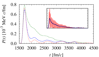
Figure 1: (color online) The emitted energy rate via EM radiation for a collision with impact parameter $b=16.2$ fm, for three orientations. In two cases the nuclear symmetry axis is parallel to the reaction plane and perpendicular (dot-dashed line) or parallel (dashed line) with respect to the incoming projectile, while in the third it is both perpendicular to the reaction plane and the incoming projectile (dotted line). These configurations are denoted by $\perp\parallel$, $\parallel$ and $\perp\perp$, respectively. We show time-averaged quantities, while in the insert, for one configuration, we also show the raw, strongly oscillating, data. The rate at which this quantity changes is directly related to the characteristic damping time, which we estimate at $500\ \mathrm{fm}/c$, leading to a width $\Gamma_{\downarrow}\approx 0.4$ MeV.

The incoming projectile excites various modes in the target nucleus and the axial symmetry of the initial ground state is lost. Because ²³⁸U is highly deformed the energy of the first $2^{+}$ is 45 keV, corresponding to a very long rotational period, and thus during simulation time considered here ($\approx 10^{-20}$ sec.) it can be considered fixed. The identification of these modes requires certain care, since during the collision the system is beyond the linear regime and the analysis using the response function is not applicable in general. However, the information about the excited nuclear modes is carried in the subsequent EM radiation leading to nuclear de-excitation. De-excitation to the ground state via photon emission requires times of about $10^{-16}$ sec., which is four orders of magnitude longer than in the current calculations. However, it is possible to compute the spectrum of the pre-equilibrium neutrons and gamma radiation, which allows the identification of the excited nuclear modes. We can accurately treat the system as a classical source of electromagnetic radiation and the time dependence of the proton current governs the rate of emission, see Refs. sup ; Baran et al. (1996); Oberacker et al. (2012):

$$P(t+r/c) = \frac{e^{2}}{\pi c}\sum_{l,m}\left|\int_{-\infty}^{\infty}{\bf b}_{lm}(k,\omega)e^{-i\omega t}d\omega\right|^{2},$$ (10)

with ${\bf b}_{lm}(k,\omega)=\int dt\,d^{3}r\,e^{-i\omega t}\mbox{{\boldmath{$\nabla$}}}\times{\bf j}({\bf r},t)j_{l}(kr)Y_{lm}^{*}(\hat{\bf r})$. Here $\omega=kc$, $j_{l}(kr)$ is the spherical Bessel function of order $l$, and ${\bf j}({\bf r},t)$ is the proton current. The emission rate $P$ is plotted in Fig. 1. The magnitude of this quantity indicates that the total amount of radiated energy during the evolution time (about $2500$ fm/c) is rather small compared to the total absorbed energy and does not exceed $1$ MeV, which is about $2-3\%$ of the deposited energy reported in Table 1 below. This implies that the effect of damping of nuclear motion due to the emitted radiation can be neglected for such short time intervals. Consequently, the decreasing intensity of the radiation, see Fig. 1, is merely related to the rearrangements of the intrinsic structure of the excited nucleus caused by damping of collective modes due to the one-body dissipation mechanism. It has to be emphasized that within the framework of the presented approach one is able to extract only a small fraction of the spreading width $\Gamma_{\downarrow}$, which is due to the one-body dissipation mechanism. The two-body effects require e.g. stochastic extension of TDSLDA which would allow for a dynamic hopping between various mean-fields, and thus could account for collisional damping as well.

TDSLDA provides the EM power spectrum sup ; Baran et al. (1996); Oberacker et al. (2012), $\frac{dE}{d\omega}={{4e^{2}}\over{c}}\sum_{l,m}|{\bf b}_{lm}(k,\omega)|^{2},$ arising from the multipole expansion in Eq. (10). This quantity is different from what one would compute within a linear response approach or first order perturbation theory, see, e.g., Refs. Winther and Alder (1979); Baur and Bertulani (1986); Emling (1994); *abe; Bertulani and Ponomarev (1999); Lanza et al. (1999); Hussein et al. (2004), which provides the excitation probability only $\propto|\int d{{}^{3}}r\rho_{tr}(\bm{r})V_{ext}(\bm{r})|^{2}$, where $\rho_{tr}(\bm{r})$ is the transition density and $V_{ext}(\bm{r})$ - the external field. $dE/d\omega$ is proportional to the excitation probability, here in the non-linear regime, and the subsequent photon emission probability as well. A typical example of the emitted EM radiation for a given impact parameter is shown in Fig. 2, here due to the internal excitation of the system alone. The EM radiation due the CM motion has been calculated separately (see Table 1 and sup ).

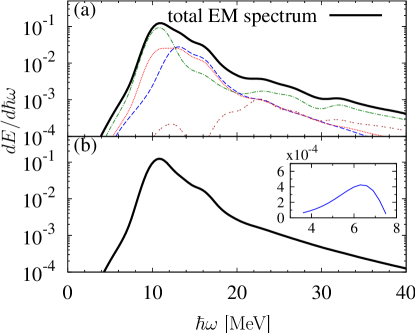
Figure 2: (color online) (a) The total energy spectrum (solid line) of emitted EM radiation, averaged over the target-projectile configurations, at the impact parameter $b=12.2$ fm. We show the total quadrupole contribution (double-dotted line), as well as the contributions from the three target-projectile orientations using the same symbols as in Fig. 1. (b) The radiation emitted from the target nucleus when only the dipole component of the projectile electromagnetic field is used. The insert shows the pygmy resonance contribution to the emitted spectrum, visible in the main figure as the slope change at low energies.

In Fig. 2(a) the emitted radiation shows a well defined maximum at energy $10-12$ MeV which corresponds to the excitation of IVGDR. We have applied a smoothing of the original calculations using the half-width of $1$ MeV. Therefore, the original separate peaks split due to the deformation of ²³⁸U merge into a single wider peak. However, at larger frequencies another local maximum exists which we associate with the isovector giant quadrupole resonance (IVGQR). In order to rule out other possibilities we have repeated the calculation by retaining only the dipole component of the electromagnetic field produced by the projectile sup . The results are shown in Fig. 2(b). In this case, the high-energy structure above 20 MeV disappears, evidence that the high energy peak is related to the IVGQR. Noticeable contribution to the total radiation is coming from the quadrupole component of radiated field.

At low energies a change of slope occurs at about $\hbar\omega\approx 7$ MeV, present at the same energy for all impact parameters and orientations, see Ref. sup . It indicates a considerable amount of strength at low energies, giving rise to an additional contribution to the EM radiation. We attribute this additional structure to the excitation of the pygmy dipole resonance (PDR). The inset of the figure 2 shows the spectrum of emitted radiation due to this mode. The contribution to the total radiated energy coming from the PDR is rather small and reads: $1.7$, $2.4$, $1.5$ and $0.8$ keV for impact parameters $12.2$, $14.6$, $16.2$ and $20.2$ fm, respectively. It corresponds to about $0.22$%, $0.5$%, $0.43$%, $0.45$% of the emitted radiation (due to internal motion) respectively. The relatively small amount of E1 strength obtained in our calculations, in the region where the PDR is expected, agrees with recent measurements Hammond et al. (2012).

The comparison between the average energy transferred to the internal motion of the target nucleus for three values of the impact parameter obtained within TDSLDA and within a simplified Goldhaber-Teller model Goldhaber and Teller (1948) presented in Table 1 shows that significantly more energy is deposited by the projectile within the TDSLDA. The Goldhaber-Teller model is equivalent to a linear response result, assuming that all isovector transition strength is concentrated in two sharp lines, corresponding to an axially deformed target. An exact QRPA approach would therefore severely underestimate the amount of internal energy deposited, one reason being the non-linearity of the response, naturally incorporated in TDSLDA. Another reason is the fact that the present microscopic framework describing the target allows for many degrees of freedom to be excited, apart from pure dipole oscillations. At the same time, the CM target energy alone is approximately the same as obtained in a simplified point particles Coulomb recoil model of both the target and projectile.

Table 1: Internal excitation energy in TD-SLDA ($E_{int}$) and in the Goldhaber-Teller model ($E_{GT}$), as well as the EM energy radiated ($E^{int}_{\gamma}$) from the excited nucleus during time interval $\delta t=2500$ fm/c after collision, for four values of impact parameters $b$ and three orientations of the nucleus with respect to the beam. We also list their respective ratios to the total transferred energy. Finally, the Goldhaber-Teller model results ($E^{*}_{GT}$) for $m^{*}=0.7m$ effective mass are presented in the last column. All energies are in MeV.

$b(fm)$	$E_{int}$	$E_{int}/E$	$E^{int}_{\gamma}$	$E^{int}_{\gamma}/E_{\gamma}$	$E_{GT}$	$E^{*}_{GT}$
12.2 $\perp||$	39.29	0.668	0.911	0.960	17.58	24.68
14.6 $\perp||$	19.2	0.608	0.567	0.963	10.32	14.51
16.2 $\perp||$	12.87	0.547	0.411	0.963	7.41	10.43
20.2 $\perp||$	5.41	0.444	0.199	0.961	3.43	4.84
12.2 $||$	25.11	0.588	0.5	0.941	12.94	18.17
14.6 $||$	13.16	0.498	0.306	0.942	7.22	10.16
16.2 $||$	8.97	0.470	0.217	0.939	5.02	7.07
20.2 $||$	3.8	0.367	0.106	0.934	2.16	3.05
12.2 $\perp\perp$	24.21	0.591	0.407	0.930	12.36	17.33
14.6 $\perp\perp$	12.58	0.513	0.245	0.929	6.65	9.34
16.2 $\perp\perp$	8.5	0.464	0.175	0.926	4.49	6.32
20.2 $\perp\perp$	3.5	0.353	0.085	0.919	1.78	2.51

The average energy radiated due to the internal excitation represents only part of the total radiated energy. (One should remember that a straightforward DFT approach provides no measure for the variance.) Also, because of the spreading of the strength due to one-body dissipation only a fraction of the energy $\Gamma_{\gamma}/\Gamma$ (where $\Gamma_{\gamma}$ is the EM-width alone and $\Gamma$ the total width of the IVGDR) is emitted as a pulse, as shown in Fig. 1. A subsequent pulse of reduced amplitude is to be expected after a delay $\approx\Gamma/(\Gamma_{\gamma}\omega_{IVGDR})\approx 10^{5}\ldots 10^{6}$ fm/c. Since our simulations times are much shorter we are not able to see emission of the second photon, as reported in experiment Boretzky et al. (2003); Ilievski et al. (2004), where two photons were measured in coincidence. In our calculations we have followed the nuclear evolution during approximately $2500$ fm/c after collision. The other component of the EM radiation arises from the CM acceleration as a result of collision (Bremsstrahlung), during the relatively short time interval $\tau_{coll}={b}/{v\gamma}$. The radiation emitted from the internal motion has a much longer time scale.

We can estimate the cross section for the emission of radiation by assuming that the asymptotic transition probability for a given impact parameter $b$ is given by ${\cal P}\propto\frac{1}{3}(\frac{E_{\gamma\perp\perp}(b)}{E_{\perp\perp}(b)}+\frac{E_{\gamma\perp||}(b)}{E_{\perp||}(b)}+\frac{E_{\gamma||}(b)}{E_{||}(b)})$. Here $E_{\perp\perp}(b)$, $E_{\perp||}(b)$ and $E_{||}(b)$ are the total energies transferred to the target nucleus during the collision at the impact parameter $b$ and for the three independent orientations. Our simulation yields $\sigma_{\gamma}=2\pi\int{\cal P}bdb\simeq 108$ mb. A detailed comparison of intensities of radiation for various impact parameters and orientations is shown in Table 1. It is evident that although the intensity of radiation decreases with increasing impact parameter, the ratio between the intensities due to the internal modes with that of the CM motion remains fairly constant and depends slightly on orientation For the orientation perpendicular to the beam and parallel to the reaction plane the target nucleus is the most efficiently excited which results in a larger ratio.

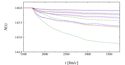
Figure 3: (color online) The number of neutrons inside the sphere of radius $15$ fm around the target nucleus as a function of time for the four impact parameters. We use the same convention as in Fig. 1 for the possible orientations. The emission rate is inverse proportional with the value of the impact parameter.

The average energy deposited in the target nucleus is of the order of the neutron separation energy. In Fig. 3 we plot the total number of neutrons inside a (smoothed) sphere of radius $15$ fm which is slightly larger than the nuclear diameter (see Ref. sup for details). For all these impact parameters neutrons can leak from the excited system. Since more energy is deposited in the nucleus with perpendicular orientation with respect to the beam, the rate of emitted neutrons is larger in that case. However, the simulation box is large enough (about 40 times bigger than the nucleus) so that during the evolution the calculations are not affected by the emitted neutrons.

We thank G.F. Bertsch for a number of discussions and reading the manuscript. We acknowledge support under U.S. DOE Grants DE-FC02-07ER41457, DE- FG02-08ER41533, NSF grant PHY-1415656, Polish National Science Centre (NCN) Grant, decision no. DEC-2013/08/A/ST3/00708, and in part by the ERANET-NuPNET grant SARFEN of the Polish National Centre for Research and Development (NCBiR). Part of this work was performed under the auspices of the National Nuclear Security Administration of the US Department of Energy at Los Alamos National Laboratory under contract No. DE-AC52-06NA25396. This research used resources of the National Energy Research Scientific Computing Center, which is supported by the Office of Science of the U.S. Department of Energy under Contract No. DE-AC02-05CH11231 and of the Oak Ridge Leadership Computing Facility at the Oak Ridge National Laboratory, which is supported by the Office of Science of the U.S. Department of Energy under Contract No. DE-AC05-00OR22725. Some of the calculations reported here have been performed at the University of Washington Hyak cluster funded by the NSF MRI Grant No. PHY-0922770. KJR was supported by the DOE Office of Science, Advanced Scientific Computing Research, under award number 58202 ”Software Effectiveness Metrics” (Lucille T. Nowell).

Supplemental material to:

Relativistic Coulomb excitation within Time Dependent Superfluid Local Density Approximation

I. Stetcu, C. Bertulani, A. Bulgac, P. Magierski and K.J. Roche

Density functional in TDSLDA and coupling to electromagnetic field

Here we present various definitions and conventions which we have used in the manuscript. The density functional is constructed from the following local densities and currents:

• density: $\rho({\bf r})=\rho({\bf r},{\bf r^{\prime}})|_{r=r^{\prime}}$

• spin density: $\vec{s}({\bf r})=\vec{s}({\bf r},{\bf r^{\prime}})|_{r=r^{\prime}}$

• current: $\vec{j}({\bf r})=\frac{1}{2i}(\vec{\nabla}-\vec{\nabla}^{\prime})\rho({\bf r},{\bf r^{\prime}})|_{r=r^{\prime}}$

• spin current (2nd rank tensor): ${\bf J}({\bf r})=\frac{1}{2i}(\vec{\nabla}-\vec{\nabla}^{\prime})\otimes\vec{s}({\bf r},{\bf r^{\prime}})|_{r=r^{\prime}}$

• kinetic energy density: $\tau({\bf r})=\vec{\nabla}\cdot\vec{\nabla}^{\prime}\rho({\bf r},{\bf r^{\prime}})|_{r=r^{\prime}}$

• spin kinetic energy density: $\vec{T}({\bf r})=\vec{\nabla}\cdot\vec{\nabla}^{\prime}\vec{s}({\bf r},{\bf r^{\prime}})|_{r=r^{\prime}}$

• anomalous density: $\chi({\bf r})=\chi({\bf r}\sigma,{\bf r^{\prime}}\sigma^{\prime})|_{r=r^{\prime},\sigma=1,\sigma^{\prime}=-\sigma}$

where

$$\rho({\bf r},{\bf r^{\prime}}) = \sum_{\mu}\left(V_{\mu}^{*}({\bf r}+)V_{\mu}({\bf r^{\prime}}+)+V_{\mu}^{*}({\bf r}-)V_{\mu}({\bf r^{\prime}}-)\right)$$

$$s_{x}({\bf r},{\bf r^{\prime}}) = \sum_{\mu}\left(V_{\mu}^{*}({\bf r}+)V_{\mu}({\bf r^{\prime}}-)+V_{\mu}^{*}({\bf r}-)V_{\mu}({\bf r^{\prime}}+)\right)$$

$$s_{y}({\bf r},{\bf r^{\prime}}) = i\sum_{\mu}\left(V_{\mu}^{*}({\bf r}+)V_{\mu}({\bf r^{\prime}}-)-V_{\mu}^{*}({\bf r}-)V_{\mu}({\bf r^{\prime}}+)\right)$$

$$s_{z}({\bf r},{\bf r^{\prime}}) = \sum_{\mu}\left(V_{\mu}^{*}({\bf r}+)V_{\mu}({\bf r^{\prime}}+)-V_{\mu}^{*}({\bf r}-)V_{\mu}({\bf r^{\prime}}-)\right)$$

$$\tau({\bf r},{\bf r^{\prime}}) = \sum_{\mu}\left(\vec{\nabla}V_{\mu}^{*}({\bf r}+)\cdot\vec{\nabla}V_{\mu}({\bf r^{\prime}}+)+\vec{\nabla}V_{\mu}^{*}({\bf r}-)\cdot\vec{\nabla}V_{\mu}({\bf r^{\prime}}-)\right)$$

$$\vec{j}({\bf r}) = -Im\left(\sum_{\mu}V_{\mu}^{*}({\bf r}+)\cdot\vec{\nabla}V_{\mu}({\bf r}+)+V_{\mu}^{*}({\bf r}-)\cdot\vec{\nabla}V_{\mu}({\bf r}-)\right)=$$

$$= Im\left(\sum_{\mu}V_{\mu}({\bf r}+)\cdot\vec{\nabla}V_{\mu}^{*}({\bf r}+)+V_{\mu}({\bf r}-)\cdot\vec{\nabla}V_{\mu}^{*}({\bf r}-)\right)$$

$$J_{x}({\bf r}) = Im\left(\frac{\partial}{\partial y}s_{z}({\bf r},{\bf r^{\prime}})-\frac{\partial}{\partial z}s_{y}({\bf r},{\bf r^{\prime}})\right)|_{r=r^{\prime}}$$

$$J_{y}({\bf r}) = Im\left(\frac{\partial}{\partial z}s_{x}({\bf r},{\bf r^{\prime}})-\frac{\partial}{\partial x}s_{z}({\bf r},{\bf r^{\prime}})\right)|_{r=r^{\prime}}$$

$$J_{z}({\bf r}) = Im\left(\frac{\partial}{\partial x}s_{y}({\bf r},{\bf r^{\prime}})-\frac{\partial}{\partial y}s_{x}({\bf r},{\bf r^{\prime}})\right)|_{r=r^{\prime}}\chi({\bf r}\sigma,{\bf r^{\prime}}\sigma^{\prime})=\sum_{\mu}V_{\mu}^{*}({\bf r}\sigma)U_{\mu}({\bf r^{\prime}}\sigma^{\prime})$$ (11)

The coupling of the nuclear system to the electromagnetic field:

$$\vec{E} = -\vec{\nabla}\phi-\frac{1}{c}\frac{\partial\vec{A}}{\partial t}$$ (12)

$$\vec{B} = \vec{\nabla}\times\vec{A}$$ (13)

requires the following transformation of proton densities and currents:

• density: $\rho_{A}({\bf r})=\rho_{A}({\bf r})$

• spin density: $\vec{s}_{A}({\bf r})=\vec{s}({\bf r})$

• current: $\vec{j}_{A}({\bf r})=\vec{j}({\bf r})-\frac{e}{\hbar c}\vec{A}\rho({\bf r})$

• spin current (2nd rank tensor): ${\bf J}_{A}({\bf r})={\bf J}({\bf r})-\frac{e}{\hbar c}\vec{A}\otimes\vec{s}({\bf r})$

• spin current (vector): $\vec{J}_{A}({\bf r})=\vec{J}({\bf r})-\frac{e}{\hbar c}\vec{A}\times\vec{s}({\bf r})$

• kinetic energy density: $\tau_{A}({\bf r})=\left(\vec{\nabla}-i\frac{e}{\hbar c}\vec{A}\right)\cdot\left(\vec{\nabla}^{\prime}+i\frac{e}{\hbar c}\vec{A}\right)\rho({\bf r},{\bf r^{\prime}})|_{r=r^{\prime}}\\ =\tau({\bf r})-2\frac{e}{\hbar c}\vec{A}\cdot\vec{j}({\bf r})+\frac{e^{2}}{\hbar^{2}c^{2}}|\vec{A}|^{2}\rho({\bf r})=\tau({\bf r})-2\frac{e}{\hbar c}\vec{A}\cdot\vec{j}_{A}({\bf r})-\frac{e^{2}}{\hbar^{2}c^{2}}|\vec{A}|^{2}\rho({\bf r})$

• spin kinetic energy density: $\vec{T}_{A}({\bf r})=\left(\vec{\nabla}-i\frac{e}{\hbar c}\vec{A}\right)\cdot\left(\vec{\nabla}^{\prime}+i\frac{e}{\hbar c}\vec{A}\right)\vec{s}({\bf r},{\bf r^{\prime}})|_{r=r^{\prime}}\\ =\vec{T}({\bf r})-2\frac{e}{\hbar c}\vec{A}^{T}\cdot{\bf J}({\bf r})+\frac{e^{2}}{\hbar^{2}c^{2}}|\vec{A}|^{2}\vec{s}({\bf r})=\vec{T}({\bf r})-2\frac{e}{\hbar c}\vec{A}^{T}\cdot{\bf J}_{A}({\bf r})-\frac{e^{2}}{\hbar^{2}c^{2}}|\vec{A}|^{2}\vec{s}({\bf r})$

As a result the proton single particle hamiltonian has the form:

$$h_{A}({\bf r})=-\vec{\nabla}_{A}\cdot\left(B({\bf r})+\vec{\sigma}\cdot\vec{C}({\bf r})\right)\vec{\nabla}_{A}+U_{A}({\bf r})+\frac{1}{2i}\left(\vec{W}({\bf r})\cdot(\vec{\nabla}_{A}\times\vec{\sigma})+\vec{\nabla}_{A}\cdot(\vec{\sigma}\times\vec{W}({\bf r}))\right)$$

$$+\vec{U}_{\sigma}^{A}({\bf r})\cdot\vec{\sigma}+\frac{1}{i}\left(\vec{\nabla}_{A}\cdot\vec{U}_{\Delta}^{A}({\bf r})+\vec{U}_{\Delta}^{A}({\bf r})\cdot\vec{\nabla}_{A}\right)$$ (15)

and

$$U_{A}({\bf r})=U({\bf r})-C^{\nabla J}\frac{e}{\hbar c}\vec{\nabla}\cdot[\vec{A}\times\vec{s}({\bf r})]-C^{\tau}\left(2\frac{e}{\hbar c}\vec{A}\cdot\vec{j}({\bf r})+\frac{e^{2}}{\hbar^{2}c^{2}}|\vec{A}|^{2}\rho({\bf r})\right)$$ (16)

$$\vec{U}_{\sigma}^{A}({\bf r})=\vec{U}_{\sigma}({\bf r})-C^{\nabla J}\frac{e}{\hbar c}\vec{\nabla}\times[\vec{A}\rho({\bf r})]-C^{sT}\left(2\frac{e}{\hbar c}\vec{A}^{T}\cdot{\bf J}({\bf r})+\frac{e^{2}}{\hbar^{2}c^{2}}|\vec{A}|^{2}\vec{s}({\bf r})\right)$$ (17)

$$\vec{U}_{\Delta}^{A}({\bf r})=\vec{U}_{\Delta}({\bf r})-C^{j}\frac{e}{\hbar c}\vec{A}\rho({\bf r})$$ (18)

$$\vec{\nabla}_{A}\cdot\left(B({\bf r})+\vec{\sigma}\cdot\vec{C}({\bf r})\right)\vec{\nabla}_{A}=\left[\vec{\nabla}_{A}\left(B({\bf r})+\vec{\sigma}\cdot\vec{C}({\bf r})\right)\right]\cdot\vec{\nabla}_{A}+$$

$$\left(B({\bf r})+\vec{\sigma}\cdot\vec{C}({\bf r})\right)\left[\Delta-i\frac{e}{\hbar c}\left(\vec{A}\cdot\vec{\nabla}_{A}+\vec{\nabla}_{A}\cdot\vec{A}\right)+\frac{e^{2}}{\hbar^{2}c^{2}}|\vec{A}|^{2}\right]$$ (19)

Numerical Implementation

We build a spatial three-dimensional Cartesian grid in coordinate space with periodic boundary conditions, and derivatives evaluated in momentum (Fourier-transformed) space. This method represents a flexible tool to describe large amplitude nuclear motion as it contains the coupling to the continuum and between single-particle and collective degrees of freedom. For the present problem, we have considered a box size of $40^{3}$ with the lattice constant 1 fm. The time step has been set to $0.076772\ \textrm{fm}/c$ with a total time interval of about $4000\ \textrm{fm}/c$. The projectile is initially placed at such a distance from the target nucleus that the collision occurs after $1600-1700\ \textrm{fm}/c$. Even though inially the projectle is far enough from the target and hence the EM fields are weak, spurious excitations produced by a sudden switch of the EM interaction at $t=0$ are possible. They were avoided by multiplying the the EM potentials in Eq. (LABEL:LW) by the smoothing function $f(t)=1/\left[1+\exp((r(t)-R_{0})/a_{0})\right]$, where $R_{0}=250$ fm, $a_{0}=50$ fm. This ensures that the EM field varies smoothly within the distance $a_{0}$, but stay approximately equal to its physical value within the distance $2R_{0}$.

Here we describe the method used to describe the Coulomb self-interaction of the target nucleus.

Consider the charge distribution $e\rho({\bf r})$:

$$\nabla^{2}\Phi({\bf r}) = 4\pi e^{2}\rho({\bf r})$$ (20)

$$\Phi({\bf r}) = \int d^{3}r^{\prime}\frac{e^{2}\rho({\bf r})}{|{\bf r}-{\bf r^{\prime}}|}$$ (21)

Note that above we have defined $\Phi$ as $e\Phi$ (note $e^{2}$ in the formula). After the Fourier transform one gets:

$$\Phi({\bf r}) = \int\frac{d^{3}k}{(2\pi)^{3}}\frac{e^{2}\rho(\vec{k})}{k^{2}}\exp(i\vec{k}\cdot{\bf r})$$ (22)

The above prescription generates however the spurious interaction between neighbouring cells.

Therefore we define the modified potential ($N_{x},N_{y},N_{z}$ denote number of equidistant lattice points in each direction, $L_{i}=N_{i}\Delta x$, $i=x,y,z$, $\Delta x$ is lattice constant):

$$f(r) = 1/r\mbox{ for }r<\sqrt{L_{x}^{2}+L_{y}^{2}+L_{z}^{2}}$$

$$f(r) = 0\mbox{ otherwise}$$ (23)

Clearly the Fourier transform is:

$$f(k)=4\pi\frac{1-\cos(k\sqrt{L_{x}^{2}+L_{y}^{2}+L_{z}^{2}})}{k^{2}}$$ (24)

and moreover

$$\Phi({\bf r}) = \int\frac{d^{3}k}{(2\pi)^{3}}\frac{e^{2}\rho(\vec{k})}{k^{2}}\exp(i\vec{k}\cdot{\bf r})=\frac{1}{27N_{x}N_{y}N_{z}}\sum_{\vec{k}\in L_{x}L_{y}L_{z}}e^{2}\rho(\vec{k})f(k)\exp(i\vec{k}\cdot{\bf r})$$ (25)

where in the last term $\rho(\vec{k})$ is the Fourier transformed density on the lattice $27L_{x}L_{y}L_{z}$. In practice it means that one has to perform forward and backward Fourier transforms on the lattice three times bigger in each direction.

This may however be avoided if one realizes that the Fourier transform of the density in the larger lattice can be expressed through the Fourier transforms in the smaller lattices:

$$\rho_{klm}(\vec{k})=\sum_{{\bf r}\in L^{3}}\rho(x,y,z)\exp\left(-i\left(k\frac{2\pi}{3L_{x}}x+l\frac{2\pi}{3L_{y}}y+m\frac{2\pi}{3L_{z}}z\right)\right)\exp(-i\vec{k}\cdot{\bf r})$$ (26)

and we need to perform 27 FFTs on the smaller lattice $L$ for $k,l,m=0,1,2$ of the following quantities:
$\rho(x,y,z)\exp\left(-i\left(k\frac{2\pi}{L_{x}}x+l\frac{2\pi}{L_{y}}y+m\frac{2\pi}{L_{z}}z\right)\right)$

Subsequently we obtain the potential through the relation:

$$\Phi({\bf r})=$$ (27)

$$= \frac{1}{27N_{x}N_{y}N_{z}}\sum_{k,l,m=0}^{2}\left[\sum_{\vec{k}\in L^{3}}e^{2}\rho_{klm}(\vec{k})f\left(\vec{k}+\left(k\frac{2\pi}{3L_{x}},l\frac{2\pi}{3L_{y}},m\frac{2\pi}{3L_{z}}\right)\right)\exp(i\vec{k}\cdot{\bf r})\right]$$

$$\times \exp\left(i\left(k\frac{2\pi}{3L_{x}}x+l\frac{2\pi}{3L_{y}}y+m\frac{2\pi}{3L_{z}}z\right)\right)$$

Dipole component of the electromagnetic field produced by the projectile

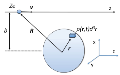
Figure 4: Coordinate system used to describe the reaction

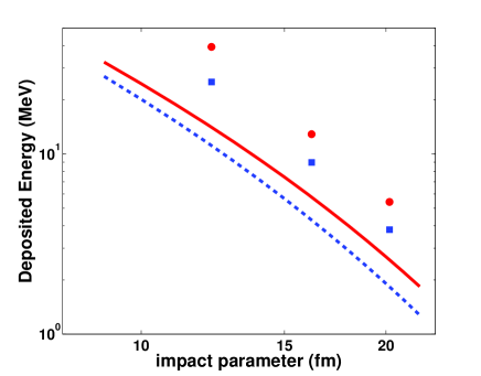
Figure 7: (color online) Energy deposited in the target nucleus ²³⁸U for three values of the impact parameter: $12.2,16.2,20.2$ fm and for two nuclear orientations: nuclear symmetry axis being parallel (squares) and perpendicular (circles) to the trajectory of incoming projectile. The same quantity is shown for the Goldhaber-Teller model, assuming that the frequencies of the dipole oscillations are $\hbar\omega=12$ MeV and $\hbar\omega=16$ MeV parallel (blue-dashed line) and perpendicular (red-solid line) to the nuclear symmetry axis, respectively.

Coordinates (see fig. 7):

$${\bf R}=(b,0,vt),\ \ \ \ {\bf r}=(x,y,z).$$ (28)

Interaction potential:

$$V_{E}({\bf r},t)=\Phi({\bf r},t)\rho_{c}({\bf r})d^{3}r,$$ (29)

where

$$\Phi({\bf r},t)={\gamma Ze\over\sqrt{(x-b)^{2}+y^{2}+\gamma^{2}(z-vt)^{2}}},$$ (30)

and $\gamma=(1-v^{2}/c^{2})^{-1/2}$. $\rho_{c}({\bf r})=e\Psi^{*}({\bf r})\Psi({\bf r})$ is the charge density of the nucleus at location ${\bf r}$ and $\Psi({\bf r})$ are proton wavefunctions . The vector potential is given by

$${\bf A}({\bf r},t)={{\bf v}\over c}\phi({\bf r},t).$$ (31)

In order to extract the dipole component we used the interaction Hamiltonian:

$${\cal H}_{int}({\bf r},t)={\gamma Ze^{2}\over\sqrt{(x-b)^{2}+y^{2}+\gamma^{2}(z-vt)^{2}}}-{\gamma Ze^{2}\over\sqrt{b^{2}+\gamma^{2}v^{2}t^{2}}},$$ (32)

where one subtracts the second term which is responsible for the c.m. scattering (i.e. monopole field).

Consequently the dipole term reads:

$${\cal H}_{{\rm E1}m}({\bf r},t)=\sqrt{\frac{2\pi}{3}}rY_{1m}\left(\hat{\bf r}\right)\frac{\gamma Ze^{2}}{\left(b^{2}+\gamma^{2}v^{2}t^{2}\right)^{3/2}}\left\{\begin{array}[c]{c}\mp b,\ \ (\mathrm{if}\ \ \ m=\pm 1)\\ \sqrt{2}vt\ \ (\mathrm{if}\ \ \ m=0)\end{array}\right.,$$ (33)

where r is the coordinate of one of the protons in the target. A sum over $m$ has to be performed, i.e.

$${\cal H}_{E1}({\bf r},t)=\sum_{i=protons}\sum_{m}{\cal H}_{E1m}({\bf r_{i}},t)=\sum_{i=protons}\sum_{m}r_{i}^{l}Y_{1m}(\hat{\bf r}_{i})f_{1m}(t),$$ (34)

where $f_{1m}(t)$ is the part of the interaction which does not involve the intrinsic structure of the nucleus:

$$f_{1m}(t)=\sqrt{\frac{2\pi}{3}}\frac{\gamma Ze^{2}}{\left(b^{2}+\gamma^{2}v^{2}t^{2}\right)^{3/2}}\left\{\begin{array}[c]{c}\mp b,\ \ (\mathrm{if}\ \ \ m=\pm 1)\\ \sqrt{2}vt\ \ (\mathrm{if}\ \ \ m=0)\end{array}\right..$$ (35)

Electromagnetic radiation from a nucleus described within TDSLDA

Let us consider the proton density and current (we use Gauss units):

$$\rho({\bf r},t) = \int_{-\infty}^{\infty}\frac{d\omega}{2\pi}\rho({\bf r},\omega)\exp(-i\omega t)$$ (36)

$$\vec{j}({\bf r},t) = \frac{1}{2\pi}\int_{-\infty}^{\infty}d\omega\vec{j}({\bf r},\omega)\exp(-i\omega t)$$ (37)

where

$$\rho({\bf r},\omega) = \int\frac{d^{3}k}{(2\pi)^{3}}\rho(\vec{k},\omega)\exp(i\vec{k}\cdot{\bf r})$$ (38)

$$\vec{j}({\bf r},\omega) = \int\frac{d^{3}k}{(2\pi)^{3}}\vec{j}(\vec{k},\omega)\exp(i\vec{k}\cdot{\bf r})$$ (39)

Maxwell equations:

$$\nabla\cdot\vec{E}({\bf r},t) = 4\pi e\rho({\bf r},t)$$ (40)

$$\nabla\cdot\vec{B}({\bf r},t) = 0$$ (41)

$$\nabla\times\vec{E}({\bf r},t) = -\frac{1}{c}\frac{\partial}{\partial t}\vec{B}({\bf r},t)$$ (42)

$$\nabla\times\vec{B}({\bf r},t) = \frac{1}{c}\left(\frac{\partial}{\partial t}\vec{E}({\bf r},t)+4\pi e\vec{j}({\bf r},t)\right)$$ (43)

and spatial Fourier transforms:

$$i\vec{k}\cdot\vec{E}(\vec{k},t) = 4\pi e\rho(\vec{k},t)$$ (44)

$$i\vec{k}\cdot\vec{B}(\vec{k},t) = 0$$ (45)

$$i\vec{k}\times\vec{E}(\vec{k},t) = -\frac{1}{c}\frac{\partial}{\partial t}\vec{B}(\vec{k},t)$$ (46)

$$i\vec{k}\times\vec{B}(\vec{k},t) = \frac{1}{c}\left(\frac{\partial}{\partial t}\vec{E}(\vec{k},t)+4\pi e\vec{j}(\vec{k},t)\right)$$ (47)

Hence clearly:

$$\vec{E} = \vec{E}_{||}+\vec{E}_{\perp}$$ (48)

$$\vec{B} = \vec{B}_{\perp}$$ (49)

where

$$\nabla\times\vec{E}_{||}({\bf r},t) = 0$$ (50)

$$\nabla\cdot\vec{E}_{\perp}({\bf r},t) = 0$$ (51)

$$\nabla\cdot\vec{B}_{\perp}({\bf r},t) = 0$$ (52)

and

$$\vec{E} = -\nabla\phi({\bf r},t)-\frac{1}{c}\frac{\partial}{\partial t}\vec{A}({\bf r},t)$$ (53)

$$\vec{B} = \nabla\times\vec{A}({\bf r},t)$$ (54)

Clearly

$$\vec{E}_{||}({\bf r},t) = -\nabla\phi({\bf r},t)-\frac{1}{c}\frac{\partial}{\partial t}\vec{A}_{||}({\bf r},t)$$ (55)

$$\vec{E}_{\perp}({\bf r},t) = -\frac{1}{c}\frac{\partial}{\partial t}\vec{A}_{\perp}({\bf r},t)$$ (56)

$$\vec{B} = \nabla\times\vec{A}_{\perp}({\bf r},t)$$ (57)

Therefore one has a freedom to choose $\vec{A}_{||}({\bf r},t)$ (gauge transformation) whereas $\vec{A}_{\perp}({\bf r},t)$ is the gauge invariant part of the vector potential.

We choose the Coulomb gauge:

$$\vec{A}_{||}({\bf r},t)=0\Leftrightarrow\vec{A}({\bf r},t)=\vec{A}_{\perp}({\bf r},t)$$ (58)

Hence

$$\vec{E}_{||}({\bf r},t) = -\nabla\phi({\bf r},t)$$ (59)

$$\vec{E}_{\perp}({\bf r},t) = -\frac{1}{c}\frac{\partial}{\partial t}\vec{A}_{\perp}({\bf r},t)$$ (60)

$$\vec{B} = \nabla\times\vec{A}_{\perp}({\bf r},t)$$ (61)

and only perpendicular components of electric and magnetic fields are responsible for emission of radiation. The important equation in this case is the fourth Maxwell equation:

$$\nabla\times\vec{B}_{\perp}({\bf r},t) = \frac{1}{c}\left(\frac{\partial}{\partial t}\vec{E}_{\perp}({\bf r},t)+4\pi e\vec{j}_{\perp}({\bf r},t)\right)+\frac{1}{c}\left(\frac{\partial}{\partial t}\vec{E}_{||}({\bf r},t)+4\pi e\vec{j}_{||}({\bf r},t)\right)$$ (62)

Since the lhs represents the vector of type $\perp$ therefore:

$$\frac{\partial}{\partial t}\vec{E}_{||}({\bf r},t)+4\pi e\vec{j}_{||}({\bf r},t)=0$$ (63)

and

$$\nabla\times\vec{B}_{\perp}({\bf r},t) = \frac{1}{c}\left(\frac{\partial}{\partial t}\vec{E}_{\perp}({\bf r},t)+4\pi e\vec{j}_{\perp}({\bf r},t)\right)$$ (64)

Substituting the potential $\vec{A}$:

$$\nabla\times\nabla\times\vec{A}_{\perp}({\bf r},t) = -\nabla^{2}\vec{A}_{\perp}({\bf r},t)=\frac{1}{c^{2}}\left(-\frac{\partial}{\partial t^{2}}\vec{A}_{\perp}({\bf r},t)+4\pi ce\vec{j}_{\perp}({\bf r},t)\right)$$ (65)

$$\nabla^{2}\vec{A}_{\perp}({\bf r},t)-\frac{1}{c^{2}}\frac{\partial}{\partial t^{2}}\vec{A}_{\perp}({\bf r},t) = -\frac{1}{c}4\pi e\vec{j}_{\perp}({\bf r},t)$$ (66)

where

$$\vec{j}_{\perp}({\bf r},t) = \vec{j}({\bf r},t)-\vec{j}_{||}({\bf r},t)=\vec{j}({\bf r},t)+\frac{1}{4\pi e}\frac{\partial}{\partial t}\vec{E}_{||}({\bf r},t)=\vec{j}({\bf r},t)-\frac{1}{4\pi e}\frac{\partial}{\partial t}\nabla\phi({\bf r},t)$$ (67)

Therefore in the Coulomb gauge

$$\vec{A}({\bf r},t) = \vec{A}_{\perp}({\bf r},t)=\frac{1}{c}\int d^{3}r^{\prime}\frac{e\vec{j}_{\perp}({\bf r^{\prime}},t-|{\bf r}-{\bf r^{\prime}}|/c)}{|{\bf r}-{\bf r^{\prime}}|}=\frac{1}{c}\int d^{3}r^{\prime}\frac{e\vec{j}_{\perp}({\bf r^{\prime}},\omega)\exp(ik|{\bf r}-{\bf r^{\prime}}|)}{|{\bf r}-{\bf r^{\prime}}|}$$ (68)

and in the far zone $r>>r^{\prime}$:

$$\vec{A}({\bf r},\omega) = \frac{\exp(ikr)}{r}\frac{1}{c}\int d^{3}r^{\prime}e\vec{j}_{\perp}({\bf r^{\prime}},\omega)\exp(-i\vec{k}\cdot{\bf r^{\prime}})=\frac{\exp(ikr)}{r}\frac{1}{c}e\vec{j}_{\perp}(\vec{k},ck)$$ (69)

where $\vec{k}=k\frac{\bf r}{r}$ and $\omega=ck$ and consequently:

$$\vec{A}({\bf r},t) = \frac{1}{2\pi}\int_{-\infty}^{\infty}d\omega\vec{A}({\bf r},\omega)\exp(-i\omega t)=\frac{e}{2\pi}\int_{-\infty}^{\infty}dk\vec{j}_{\perp}(\vec{k},ck)\frac{\exp(ik(r-ct)}{r}$$ (70)

Consequently since $\vec{B}=\nabla\times\vec{A}$ we get:

$$\vec{B}({\bf r},\omega)=\nabla\times\vec{A}({\bf r},\omega)=\nabla\times\frac{1}{c}\int d^{3}r^{\prime}\frac{e\vec{j}_{\perp}({\bf r^{\prime}},\omega)\exp(ik|{\bf r}-{\bf r^{\prime}}|)}{|{\bf r}-{\bf r^{\prime}}|}=$$ (71)

$$= \frac{1}{c}\int d^{3}r^{\prime}\frac{ik({\bf r}-{\bf r^{\prime}})\times e\vec{j}_{\perp}({\bf r^{\prime}},\omega)\exp(ik|{\bf r}-{\bf r^{\prime}}|)}{|{\bf r}-{\bf r^{\prime}}|^{2}}-\frac{1}{c}\int d^{3}r^{\prime}\frac{({\bf r}-{\bf r^{\prime}})\times e\vec{j}_{\perp}({\bf r^{\prime}},\omega)\exp(ik|{\bf r}-{\bf r^{\prime}}|)}{|{\bf r}-{\bf r^{\prime}}|^{3}}$$

$$= \frac{1}{c}\int d^{3}r^{\prime}\frac{ik({\bf r}-{\bf r^{\prime}})\times e\vec{j}({\bf r^{\prime}},\omega)\exp(ik|{\bf r}-{\bf r^{\prime}}|)}{|{\bf r}-{\bf r^{\prime}}|^{2}}-\frac{1}{c}\int d^{3}r^{\prime}\frac{({\bf r}-{\bf r^{\prime}})\times e\vec{j}({\bf r^{\prime}},\omega)\exp(ik|{\bf r}-{\bf r^{\prime}}|)}{|{\bf r}-{\bf r^{\prime}}|^{3}},$$

where in the last line we have used the fact that rotation of the vector of type $||$ is zero. For the electric field:

$$\vec{E}_{\perp}({\bf r},\omega) = \frac{i\omega}{c}\vec{A}({\bf r},\omega)=\frac{i\omega}{c^{2}}\int d^{3}r^{\prime}\frac{e\vec{j}_{\perp}({\bf r^{\prime}},\omega)\exp(ik|{\bf r}-{\bf r^{\prime}}|)}{|{\bf r}-{\bf r^{\prime}}|}$$ (72)

$$\vec{E}_{||}({\bf r},\omega) = -\nabla\phi({\bf r},\omega)=-\nabla\int d^{3}r^{\prime}\frac{e\rho({\bf r^{\prime}},\omega)}{|{\bf r}-{\bf r^{\prime}}|}$$ (73)

Hence in the far zone $r>>r^{\prime}$ one gets:

$$\vec{B}({\bf r},\omega) = \frac{ie}{c}\frac{\exp(ikr)}{r}\int d^{3}r^{\prime}\vec{k}\times\vec{j}_{\perp}({\bf r^{\prime}},\omega)\exp(-i\vec{k}\cdot{\bf r^{\prime}})=\frac{ie}{c}\frac{\exp(ikr)}{r}\vec{k}\times\vec{j}(\vec{k},\omega)$$ (74)

$$\vec{E}({\bf r},\omega) = \vec{E}_{\perp}({\bf r},\omega)+\vec{E}_{||}({\bf r},\omega)=\frac{\exp(ikr)}{r}\frac{i\omega}{c^{2}}e\vec{j}_{\perp}(\vec{k},ck)=\frac{ie}{c}\frac{\exp(ikr)}{r}k\vec{j}_{\perp}(\vec{k},ck)$$ (75)

$$= \frac{ie}{c}\frac{\exp(ikr)}{r}k(\vec{j}(\vec{k},ck)-\vec{j}_{||}(\vec{k},ck))=\frac{ie}{c}\frac{\exp(ikr)}{r}\left((\vec{k}\cdot\frac{\bf r}{r})\vec{j}(\vec{k},ck)-(\vec{k}\cdot\vec{j}(\vec{k},ck))\frac{\bf r}{r}\right)$$ (76)

$$= \frac{ie}{c}\frac{\exp(ikr)}{r}\frac{\bf r}{r}\times\left(\vec{j}(\vec{k},\omega)\times\vec{k}\right)$$ (77)

and consequently:

$$\vec{B}({\bf r},t)=\frac{1}{2\pi}\int_{-\infty}^{\infty}d\omega\vec{B}({\bf r},\omega)\exp(-i\omega t) = \frac{ie}{2\pi}\int_{-\infty}^{\infty}dk\vec{k}\times\vec{j}(\vec{k},ck)\frac{\exp(ik(r-ct))}{r}$$ (78)

$$= \frac{ie}{c}\int_{-\infty}^{\infty}\frac{d\omega}{2\pi}\vec{k}\times\vec{j}(\vec{k},\omega)\frac{\exp(-i\omega(t-r/c))}{r}$$ (79)

$$\vec{E}({\bf r},t)=\frac{1}{2\pi}\int_{-\infty}^{\infty}d\omega\vec{E}({\bf r},\omega)\exp(-i\omega t) = \frac{ie}{2\pi}\frac{\bf r}{r}\times\int_{-\infty}^{\infty}dk\left(\vec{j}(\vec{k},ck)\times\vec{k}\right)\frac{\exp(ik(r-ct))}{r}$$ (80)

$$= \frac{ie}{c}\frac{\bf r}{r}\times\int_{-\infty}^{\infty}\frac{d\omega}{2\pi}\left(\vec{j}(\vec{k},\omega)\times\vec{k}\right)\frac{\exp(-i\omega(t-r/c))}{r}$$ (81)

Note that in the above expressions $\vec{k}$ and $\omega$ are related: $\omega=c|\vec{k}|$.

Poynting vector reads $\vec{S}=\frac{c}{4\pi}\vec{E}\times\vec{B}$ and thus:

$$\vec{S}(t) = \frac{c}{4\pi(2\pi)^{2}}\int_{-\infty}^{\infty}d\omega\int_{-\infty}^{\infty}d\omega^{\prime}\vec{E}({\bf r},\omega)\times\vec{B}({\bf r},\omega)\exp(-i(\omega+\omega^{\prime})t)$$ (82)

$$= \frac{c}{4\pi(2\pi)^{2}}\int_{-\infty}^{\infty}d\omega\int_{-\infty}^{\infty}d\omega^{\prime}\vec{E}({\bf r},\omega)\times\vec{B}^{*}({\bf r},\omega^{\prime})\exp(-i(\omega-\omega^{\prime})t)$$

$$= \frac{e^{2}}{4\pi(2\pi)^{2}cr^{2}}\frac{\bf r}{r}\int_{-\infty}^{\infty}d\omega\int_{-\infty}^{\infty}d\omega^{\prime}(\vec{k}\times\vec{j}(\vec{k},\omega))\cdot(\vec{k^{\prime}}\times\vec{j}^{*}(\vec{k^{\prime}},\omega^{\prime}))\exp(-i(\omega-\omega^{\prime})t+i(k-k^{\prime})r)$$

$$= \frac{e^{2}}{4\pi cr^{2}}\frac{\bf r}{r}\left|\int_{-\infty}^{\infty}\frac{d\omega}{2\pi}(\vec{k}\times\vec{j}(\vec{k},\omega))\exp(-i\omega t+ikr)\right|^{2}$$ (83)

$$= \frac{c}{4\pi}\frac{\bf r}{r}\left|\int_{-\infty}^{\infty}\frac{d\omega}{2\pi}\vec{B}({\bf r},\omega)\exp(-i\omega t)\right|^{2}$$ (84)

Energy per unit time emitted to the angle $d\Omega$ reads:

$$dP(t) = \vec{S}(t)\cdot\frac{\bf r}{r}r^{2}d\Omega=\frac{e^{2}}{4\pi c}\left|\int\frac{d\omega}{2\pi}(\vec{k}\times\vec{j}(\vec{k},\omega))\exp(-i\omega t+ikr)\right|^{2}d\Omega$$ (85)

Hence

$$\frac{dP}{d\Omega}(t) = \frac{e^{2}}{4\pi c}\left|\int_{-\infty}^{\infty}\frac{d\omega}{2\pi}(\vec{k}\times\vec{j}(\vec{k},\omega))\exp(-i\omega(t-r/c))\right|^{2}=\frac{c}{4\pi}r^{2}\left|\vec{B}({\bf r},t)\right|^{2}$$ (86)

Note that the radiation at time $t$ is given by the current at time $t-r/c$, thus a simple time shift, which we can discard. Therefore the total amount of radiated energy at the angle $d\Omega$ reads:

$$\int_{-\infty}^{\infty}\frac{dP}{d\Omega}(t)dt = \frac{c}{4\pi}r^{2}\int_{-\infty}^{\infty}\left|\vec{B}({\bf r},t)\right|^{2}dt=\frac{c}{4\pi}r^{2}\int_{-\infty}^{\infty}\vec{B}({\bf r},t)\cdot\int_{-\infty}^{\infty}\frac{d\omega}{2\pi}\vec{B}({\bf r},\omega)\exp(-i\omega t)dt$$ (87)

$$= \frac{c}{4\pi}r^{2}\int_{-\infty}^{\infty}\frac{d\omega}{2\pi}\vec{B}({\bf r},-\omega)\cdot\vec{B}({\bf r},\omega)=\frac{c}{4\pi}r^{2}\int_{-\infty}^{\infty}\frac{d\omega}{2\pi}\vec{B}^{*}({\bf r},\omega)\cdot\vec{B}({\bf r},\omega)$$

which gives the spectral decomposition of emitted radiation:

$$\int_{-\infty}^{\infty}\frac{dP}{d\Omega}(t)dt = \frac{c}{8\pi^{2}}r^{2}\int_{-\infty}^{\infty}d\omega\left|\vec{B}({\bf r},\omega)\right|^{2}=\frac{c}{4\pi^{2}}r^{2}\int_{0}^{\infty}d\omega\left|\vec{B}({\bf r},\omega)\right|^{2}$$ (88)

Hence the energy emitted at the angle $\Omega$ at frequency $\omega$ reads:

$$\frac{dE}{d\Omega d\omega}(\omega) = \frac{e^{2}}{4\pi^{2}c}\left|\vec{k}\times\vec{j}(\vec{k},\omega)\right|^{2}=\frac{e^{2}}{4\pi^{2}c}\left|\int d^{3}r\left(\nabla\times\vec{j}({\bf r},\omega)\right)\exp(-i\vec{k}\cdot{\bf r})\right|^{2}$$ (89)

In order to calculate the quantities given by the expressions: (86) (89) we use the multipole expansion. Namely, let us consider eq. (89):

$$\frac{dE}{d\omega} = \int\frac{dE}{d\Omega d\omega}(\omega)d\Omega=\int\frac{e^{2}}{4\pi^{2}c}\left|\vec{k}\times\vec{j}(\vec{k},\omega)\right|^{2}d\Omega$$ (90)

$$= \frac{e^{2}}{4\pi^{2}c}\int\left|\int d^{3}r\int_{-\infty}^{\infty}dt\left(\vec{\nabla}\times\vec{j}({\bf r},t)\right)\exp(-i\vec{k}\cdot{\bf r}+i\omega t)\right|^{2}d\Omega$$ (91)

Let us denote:

$$\vec{\nabla}\times\vec{j}({\bf r},t) = \vec{b}({\bf r},t)$$ (92)

$$\vec{\nabla}\times\vec{j}({\bf r},\omega) = \vec{b}({\bf r},\omega)$$ (93)

We expand $\exp(-i\vec{k}\cdot{\bf r})$:

$$\exp(-i\vec{k}\cdot{\bf r})=4\pi\sum_{l,m}(-i)^{l}j_{l}(kr)Y_{lm}(\hat{k})Y_{lm}^{*}(\hat{r})$$ (94)

and consequently we get

$$\frac{dE}{d\omega} = \frac{e^{2}}{4\pi^{2}c}\int\left|\int d^{3}r\int_{-\infty}^{\infty}dt\left(\vec{b}({\bf r},t)4\pi\sum_{l,m}(-i)^{l}j_{l}(kr)Y_{lm}(\hat{k})Y_{lm}^{*}(\hat{r})\right)\exp(i\omega t)\right|^{2}d\Omega$$ (95)

$$= \frac{e^{2}}{4\pi^{2}c}\int\left|\int_{-\infty}^{\infty}dt4\pi\sum_{l,m}(-i)^{l}\vec{b}_{lm}(\vec{k},t)Y_{lm}(\hat{k})\exp(i\omega t)\right|^{2}d\Omega$$ (96)

$$= \frac{e^{2}}{4\pi^{2}c}\int\left|4\pi\sum_{l,m}(-i)^{l}\vec{b}_{lm}(\vec{k},\omega)Y_{lm}(\hat{k})\right|^{2}d\Omega$$ (97)

where

$$\vec{b}_{lm}(k,t) = \int d^{3}r\vec{b}({\bf r},t)j_{l}(kr)Y_{lm}^{*}(\hat{r})$$ (98)

$$\vec{b}_{lm}(k,\omega) = \int_{-\infty}^{\infty}\vec{b}_{lm}(k,t)\exp(i\omega t)dt$$ (99)

Note that $\vec{b}_{lm}$ is a function of $k$ (not $\vec{k}$) and

$$\frac{dE}{d\omega} = \frac{e^{2}}{4\pi^{2}c}(4\pi)^{2}\int\left(\sum_{l,m,l^{\prime},m^{\prime}}(-i)^{l}i^{l^{\prime}}\left(\vec{b}_{lm}(k,\omega)\cdot\vec{b}_{l^{\prime}m^{\prime}}^{*}(k,\omega)\right)Y_{lm}(\hat{k})Y_{l^{\prime}m^{\prime}}^{*}(\hat{k})\right)d\Omega$$ (100)

$$= \frac{e^{2}}{4\pi^{2}c}(4\pi)^{2}\sum_{l,m}|\vec{b}_{lm}(k,\omega)|^{2}=\frac{4e^{2}}{c}\sum_{l,m}|\vec{b}_{lm}(k,\omega)|^{2}$$ (101)

The above equation is used to calculate the spectrum of emitted radiation. In practice one needs only few multipoles. The contribution coming from $l=4$ term is already negligibly small.

In order to determine the rate of emitted radiation let us consider eq. (86):

$$P(t+r/c) = \int\frac{dP}{d\Omega}(t+r/c)d\Omega=\frac{e^{2}}{4\pi c}\int\left|\int_{-\infty}^{\infty}\frac{d\omega}{2\pi}(\vec{k}\times\vec{j}(\vec{k},\omega))\exp(-i\omega t)\right|^{2}d\Omega$$ (102)

$$= \frac{e^{2}}{4\pi c}\int\left|\int_{-\infty}^{\infty}\frac{d\omega}{2\pi}\left(\int d^{3}r(\vec{\nabla}\times\vec{j}({\bf r},\omega))\exp(-i\vec{k}\cdot{\bf r})\right)\exp(-i\omega t)\right|^{2}d\Omega$$ (103)

$$= \frac{e^{2}}{4\pi c}\int\left|\int_{-\infty}^{\infty}\frac{d\omega}{2\pi}\left(\int d^{3}r4\pi\sum_{l,m}(-i)^{l}\vec{b}({\bf r},\omega)j_{l}(kr)Y_{lm}(\hat{k})Y_{lm}^{*}(\hat{r})\right)\exp(-i\omega t)\right|^{2}d\Omega$$ (104)

$$= \frac{e^{2}}{4\pi c}\int\left|\int_{-\infty}^{\infty}\frac{d\omega}{2\pi}\left(4\pi\sum_{l,m}(-i)^{l}\vec{b}_{lm}(k,\omega)Y_{lm}(\hat{k})\right)\exp(-i\omega t)\right|^{2}d\Omega$$

$$= \frac{e^{2}}{4\pi c}\int_{-\infty}^{\infty}\frac{d\omega}{2\pi}\int_{-\infty}^{\infty}\frac{d\omega^{\prime}}{2\pi}\left((4\pi)^{2}\int d\Omega\sum_{l,m,l^{\prime},m^{\prime}}(-i)^{l}i^{l^{\prime}}\left(\vec{b}_{lm}(k,\omega)\cdot\vec{b}_{l^{\prime}m^{\prime}}^{*}(k^{\prime},\omega^{\prime})\right)Y_{lm}(\hat{k})Y_{l^{\prime}m^{\prime}}^{*}(\hat{k})\right)\times$$

$$\times \exp(-i(\omega-\omega^{\prime})t)$$ (106)

Note that in the last two lines of the above expression $\hat{k}=\hat{k^{\prime}}$ because the vectors $\vec{k},\vec{k}^{\prime}$ differ only by length ($\omega=ck,\omega^{\prime}=ck^{\prime}$) but have the same direction specified by the angle $\Omega$. Therefore:

$$P(t+r/c) = \frac{e^{2}}{4\pi c}\int_{-\infty}^{\infty}\frac{d\omega}{2\pi}\int_{-\infty}^{\infty}\frac{d\omega^{\prime}}{2\pi}\left((4\pi)^{2}\sum_{l,m}\left(\vec{b}_{lm}(k,\omega)\cdot\vec{b}_{lm}^{*}(k^{\prime},\omega^{\prime})\right)\right)\exp(-i(\omega-\omega^{\prime})t)$$ (107)

$$= \frac{e^{2}}{\pi c}\sum_{l,m}\left|\int_{-\infty}^{\infty}\vec{b}_{lm}(k,\omega)\exp(-i\omega t)d\omega\right|^{2}$$ (108)

The last equation is used in practice to calculate the rate of emitted radiation.

The above prescriptions work efficiently if one considers the radiation emitted due to internal nuclear excitation. However in order to determine the contribution coming from the CM motion of the nucleus the simpler formula can be derived. In this case the proton current reads:

$$\vec{j}_{p}({\bf r},t)=\vec{V}(t)\delta({\bf r}-{\bf r}_{0}(t))$$ (109)

Then

$$\vec{A}({\bf r},\omega) = \frac{\exp(ikr)}{r}\frac{Ze}{c}\int d^{3}r^{\prime}\vec{j}_{p}({\bf r^{\prime}},\omega)\exp(-i\vec{k}\cdot{\bf r^{\prime}})$$ (110)

$$= \frac{\exp(ikr)}{r}\frac{1}{c}Ze\int_{-\infty}^{\infty}dt\exp(i\omega t)\vec{V}(t)\exp(-i\vec{k}\cdot{\bf r}_{0}(t))$$ (111)

where

$$\vec{j}_{p}(\vec{k},\omega) = \int_{-\infty}^{\infty}dt\exp\left(i\omega\left(t-\frac{1}{c}\vec{n}\cdot{\bf r}_{0}(t)\right)\right)\vec{V}(t)$$ (112)

$$\approx \int_{-\infty}^{\infty}dt\exp(i\omega t)\vec{V}\left(t+\frac{1}{c}\vec{n}\cdot{\bf r}_{0}(t)\right)$$ (113)

$$\approx \int_{-\infty}^{\infty}dt\exp(i\omega t)\vec{V}(t)=\vec{V}(\omega),$$ (114)

where $\omega=ck$. The approximation was made above that the velocity is small and the movement of the nucleus is negligible. Therefore the possible perturbation of the radiation due to the change of nucleus position can be neglected.

Consequently:

$$\vec{B}({\bf r},\omega)=\frac{iZe}{c}\frac{\exp(ikr)}{r}\vec{k}\times\vec{V}(\omega)$$ (115)

and

$$\vec{B}({\bf r},t) = \int_{-\infty}^{\infty}\frac{d\omega}{2\pi}\vec{B}({\bf r},\omega)\exp(-i\omega t)$$ (116)

$$= \frac{iZe}{c^{2}}\frac{1}{r}\int_{-\infty}^{\infty}\frac{d\omega}{2\pi}\exp\left(-i\omega\left(t-\frac{r}{c}\right)\right)\omega\vec{n}\times\vec{V}(\omega)$$ (117)

$$= -\frac{Ze}{c^{2}}\frac{1}{r}\frac{d}{dt}\int_{-\infty}^{\infty}\frac{d\omega}{2\pi}\exp\left(-i\omega\left(t-\frac{r}{c}\right)\right)\vec{n}\times\vec{V}(\omega)$$ (118)

$$= -\frac{Ze}{c^{2}}\frac{1}{r}\vec{n}\times\frac{d}{dt}\vec{V}\left(t-\frac{r}{c}\right)$$ (119)

Therefore

$$\frac{dP}{d\Omega}(t) = \frac{c}{4\pi}r^{2}\left|\vec{B}({\bf r},t)\right|^{2}=\frac{1}{4\pi c^{3}}(Ze)^{2}\left|\frac{dV\left(t-\frac{r}{c}\right)}{dt}\right|^{2}\sin^{2}\theta$$ (120)

and

$$P(t) = \frac{2}{3}\frac{(Ze)^{2}}{c^{3}}\left|\frac{dV\left(t-\frac{r}{c}\right)}{dt}\right|^{2}$$ (121)

Spectral decomposition:

$$\frac{dE}{d\Omega d\omega}=\frac{(Ze)^{2}}{4\pi^{2}c}|\vec{k}\times\vec{V}(\omega)|^{2}$$ (122)

and integrating over angles

$$\frac{dE}{d\omega}=\frac{2}{3\pi}\frac{(Ze)^{2}}{c}k^{2}|\vec{V}(\omega)|^{2}=\frac{2}{3\pi}\frac{(Ze)^{2}}{c^{3}}\omega^{2}|\vec{V}(\omega)|^{2}=\frac{2}{3\pi}\frac{(Ze)^{2}}{c^{3}}\left|\frac{d\vec{V}}{dt}(\omega)\right|^{2}$$ (123)

where $\frac{d\vec{V}}{dt}(\omega)$ is the Fourier transform of acceleration:

$$\frac{d\vec{V}}{dt}(\omega)=\int dt\frac{d\vec{V}}{dt}(t)\exp(i\omega t)$$ (124)

The above derivation assumes that the moving nucleus can be treated as a point-like particle. This is a reasonable approximation although it is not difficult to include suitable corrections. Let us consider the proton current in the form:

$$\vec{j}_{p}({\bf r},t)=\vec{V}(t)\rho({\bf r}-{\bf r}_{0}(t))$$ (125)

Using the same assumption as before, ie. that the motion is nonrelativistic and movement in space is negligible one gets:

$$\vec{j}_{p}(\vec{k},\omega) = \vec{V}(\omega)\rho(\vec{k})$$ (126)

and (see (89)):

$$\int\frac{dE}{d\Omega d\omega}d\Omega = \frac{(Ze)^{2}}{4\pi^{2}c}|\vec{k}\times\vec{V}(\omega)\rho(\vec{k})|^{2}d\Omega=\frac{(Ze)^{2}}{4\pi^{2}c}\frac{1}{c^{2}}\int|\vec{n}\times\omega\vec{V}(\omega)\rho(\vec{k})|^{2}d\Omega$$ (127)

$$= \frac{(Ze)^{2}}{4\pi^{2}c^{3}}\int\left|\vec{n}\times\frac{d\vec{V}}{dt}(\omega)\rho(\vec{k})\right|^{2}d\Omega$$ (128)

where $\vec{n}=\frac{\bf r}{r}$. In the case of spherical density distribution it simplifies to:

$$\int\frac{dE}{d\Omega d\omega}d\Omega = \frac{(Ze)^{2}}{4\pi^{2}c^{3}}\int\left|\vec{n}\times\frac{d\vec{V}}{dt}(\omega)\right|^{2}|\rho(k)|^{2}d\Omega=\frac{2}{3\pi}\frac{(Ze)^{2}}{c^{3}}\left|\frac{d\vec{V}}{dt}(\omega)\right|^{2}|\rho(k)|^{2}$$ (129)

The above expressions can be used to determine the spectrum of emitted radiation. In the Figures 5 and 6 the contributions to the energy spectrum coming from dipole and quadrupole terms are plotted for $3$ values of impact parameter. The difference between the figures originates from two different smoothing widths that have been applied. Namely, the original curves have been convoluted with gaussians of widths $1$ MeV (Fig. 5) and $0.5$ MeV (Fig. 6 ).

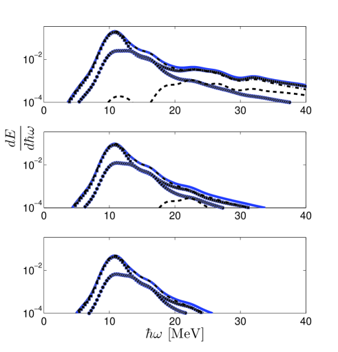
Figure 5: (color online) The energy spectrum of emitted electromagnetic radiation due to internal excitation of the target nucleus, caused by the collision at the impact parameters $b=12.2$ fm (upper subfigure), $b=16.2$ and $b=20.2$ (lowest subfigure) . The contributions from two orientations of the target nucleus are shown: perpendicular (squares) and parallel (circles) with respect to the incoming projectile. Dotted dashed line represents the dipole component of the radiation. Dashed line represents the quadrupole component of the radiation. In this case the smoothing width of the original curves was set to $1$ MeV.

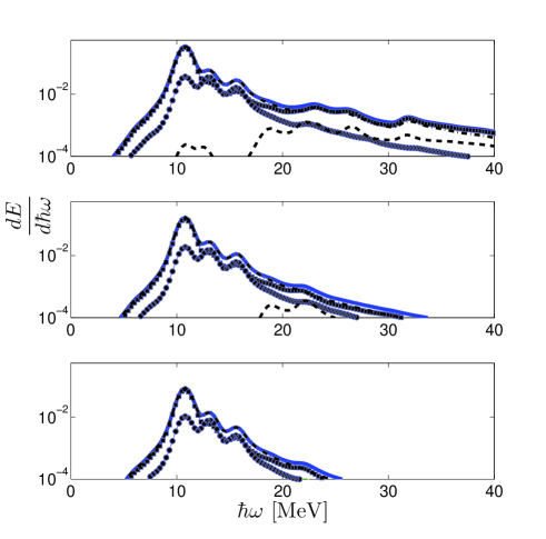
Figure 6: (color online) The same as in the Fig. 5, but in this case the smoothing width of the original curves was set to $0.5$ MeV.

For the radiation caused by the CM acceleration after collision the decomposition into multipoles is not useful and one can apply instead eqs. (LABEL:cmpower,cmspectr). The emission occurs within much shorter time scale governed by the collision time $\tau_{coll}=\frac{b}{v\gamma}$. The results are plotted in the Figs. 8, 9, 10.

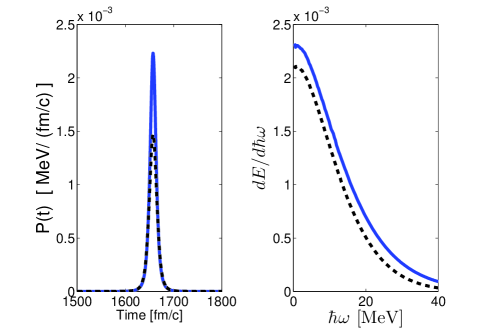
Figure 8: (color online) The gamma emission rate (left panel) due to bremsstrahlung for the collision at the impact parameter $b=12.2$fm. The right panel shows the energy spectrum emitted. Solid and dashed lines correspond to the perpendicular and parallel orientation of the target nucleus with respect to incoming projectile.

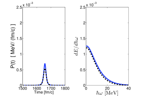
Figure 9: (color online) The same as in the Fig. 8, but for the impact parameter $b=16.2$fm.

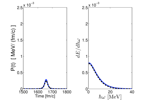
Figure 10: (color online) The same as in the Fig. 8, but for the impact parameter $b=20.2$fm.

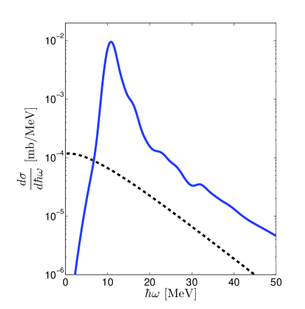
Figure 11: (color online) The contributions to the cross section with respect to gamma emission during $2500$ fm/c after collision. The dashed line represents the Bremsstrahlung contribution. The solid line shows the contribution from intrinsic excitation modes.

Dipole dynamics and neutron emission

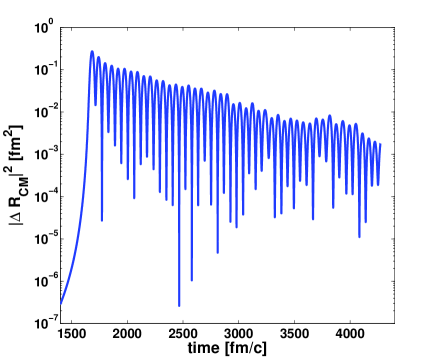
Figure 12: (color online) The distance squared between the CM of protons and the total nuclear CM: $|\Delta R_{CM}|^{2}$ as a function of time. The impact parameter is $b=12.2$ fm, and the nuclear symmetry axis of the target is perpendicular to the projectile’s trajectory. The slope does not depend on the orientation and the impact parameter. The numerical fit to the maxima (squared amplitudes of dipole oscillations) with the function $\exp(-t/\tau)$ yields $\tau\approx 500$ fm/c.

The framework of TDSLDA allows to calculate various one body observables. In this case the most important is the nuclear dipole moment. Only two components of the dipole moment, lying in the reaction plane, can oscillate as a result of collision. In the Figs. 13, 14, 15 these two components of the dipole moment have been plotted.

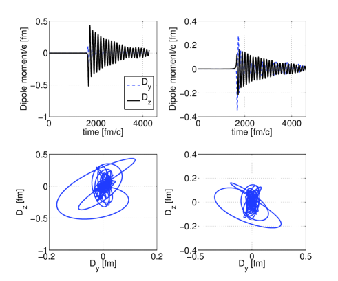
Figure 13: (color online) Two components of the dipole moment: $D_{z}$ and $D_{y}$ as a function of time. The left and right subfigures correspond to the collision with projectile moving along the $y$-axis and $z$-axis , respectively. Impact parameter: $b=12.2$fm.

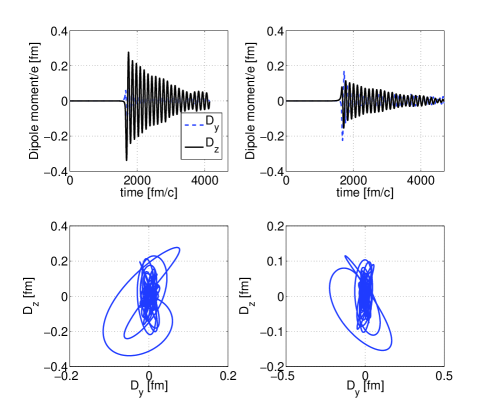
Figure 14: (color online) The same as in the Fig. 13, but for the impact parameter $b=16.2$fm.

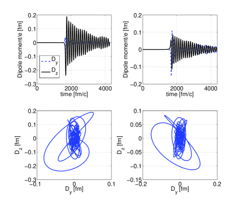
Figure 15: (color online) The same as in the Fig. 13, but for the impact parameter $b=20.2$fm.

During the time evolution the nucleus can emit particles. In order to investigate this effect we have calculated the number of neutrons/protons within shells of various radii. As one can see from the Figs. 16, 17, 18, 19 the number of protons in the shells outside the nucleus is negligible. Moreover this proton number is approximately constant which indicate that we rather probe the tale of the proton distribution than the emission process. On the contrary the situation is different for neutrons. The number of neutrons in the smaller shell is much larger, although it is also approximately constant. However in the larger shell the number of neutrons is constantly increasing in time with a fairly constant average rate. It indicates that the neutron emission occurs as a result of Coulomb excitation process.

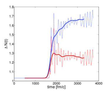
Figure 16: (color online) The number of neutrons present within the shell with inner radius $10$fm and outer radius $15$fm (red line). The number of neutrons present within the shell with inner radius $10$fm and outer radius $20$fm (blue line). Thin line corresponds to the actual number of neutrons, whereas the thick line denotes the average value. The plot corresponds to the collision with the target nucleus symmetry axis perpendicular to the trajectory of the incoming projectile. The impact parameter $b=12.2$ fm.

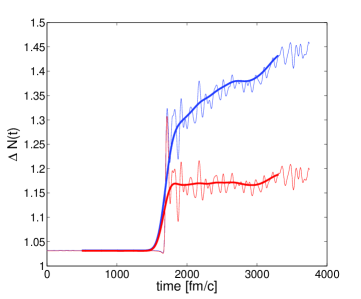
Figure 17: (color online) The same as in the Fig. 16, but for the nuclear orientation parallel with respect to the incoming projectile.

Figure 18: (color online) The same as in the Fig. 16, but for protons.

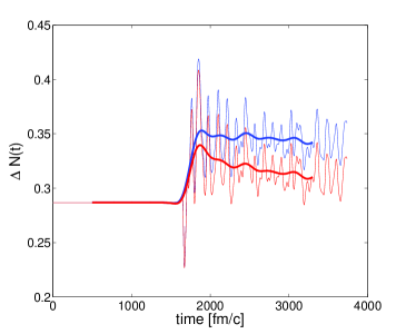
Figure 19: (color online) The same as in the Fig. 17, but for protons.