Low discrepancy constructions in the triangle

Abstract

Most quasi-Monte Carlo research focuses on sampling from the unit cube. Many problems, especially in computer graphics, are defined via quadrature over the unit triangle. Quasi-Monte Carlo methods for the triangle have been developed by Pillards and Cools, (2005) and by Brandolini et al., (2013). This paper presents two QMC constructions in the triangle with a vanishing discrepancy. The first is a version of the van der Corput sequence customized to the unit triangle. It is an extensible digital construction that attains a discrepancy below $12/{\sqrt{N}}$. The second construction rotates an integer lattice through an angle whose tangent is a quadratic irrational number. It attains a discrepancy of $O(\log(N)/N)$ which is the best possible rate. Previous work strongly indicated that such a discrepancy was possible, but no constructions were available. Scrambling the digits of the first construction improves its accuracy for integration of smooth functions. Both constructions also yield convergent estimates for integrands that are Riemann integrable on the triangle without requiring bounded variation.

Keywords : Quasi-Monte Carlo Method; Discrepancy on Triangle; Quadrature error.

1 Introduction

The problem we consider here is numerical integration over a triangular domain, using quasi-Monte Carlo (QMC) sampling. Such integrals commonly arise in graphical rendering. Classical quadrature methods find a set of points $\boldsymbol{x}_{1},\dots,\boldsymbol{x}_{N}$ in the triangle and weights $w_{i}\in\real$ so that $\sum_{i=1}^{N}w_{i}f(\boldsymbol{x}_{i})$ correctly integrates a class of polynomials $f$. Lyness and Cools, (1994) give a survey.

Classical rules often do poorly on non-smooth integrands. It is also difficult to estimate error for them and there is little freedom to choose $N$. As a result, QMC sampling, which equidistributes sample points through the domain of interest is attractive.

QMC sampling is well developed for numerical integration of functions defined on the unit cube $[0,1]^{d}$. The quantity $\mu=\int_{[0,1]^{d}}f(\boldsymbol{x})\mathrm{\,d}\boldsymbol{x}$ is approximated by an equal weight rule $\hat{\mu}_{N}=(1/N)\sum_{i=1}^{N}f(\boldsymbol{x}_{i})$ for carefully chosen $\boldsymbol{x}_{i}\in[0,1]^{d}$. The accuracy of QMC is customarily measured via the Koksma-Hlawka inequality (see Niederreiter, (1992)). There $|\hat{\mu}_{N}-\mu|\leqslant D_{N}^{*}(\boldsymbol{x}_{1},\dots,\boldsymbol{x}_{N})\times V_{\mathrm{HK}}(f)$ where $D_{N}^{*}$ is the star discrepancy (a measure of non-uniformity) of the sample points and $V_{\mathrm{HK}}$ is the total variation of $f$ in the sense of Hardy and Krause.

The usual approach to sampling these domains is to apply a mapping $\phi$ from $[0,1]^{d}$ to the domain $D$ of interest. The mapping is such that if $\boldsymbol{x}\sim\mathbf{U}([0,1]^{d})$ (uniform distribution) then $\phi(\boldsymbol{x})\sim\mathbf{U}(D)$. There are typically several choices for such mappings and the dimension $d$ of the cube is not necessarily equal to the dimension of $D$. With such a mapping in hand we may generate QMC points $\boldsymbol{x}_{i}\in[0,1]^{d}$ and use $\phi(\boldsymbol{x}_{i})$ as sample points in $D$.

Using this approach we may estimate $\mu=\int_{D}g(\boldsymbol{x})\mathrm{\,d}\boldsymbol{x}$ by $(1/n)\sum_{i=1}^{n}f(\boldsymbol{x}_{i})$ where $f(\boldsymbol{x})=g(\phi(\boldsymbol{x}))$. The difficulty is that the composite function $f=g\circ\phi$ may not be well suited to QMC; it may have cusps or singularities or discontinuities. These features may diminish the performance of QMC. At a minimum, they make it more difficult to analyze QMC’s performance.

Recently Brandolini et al., (2013) presented a version of the Koksma-Hlawka inequality for the simplex. They devised a measure of variation for the simplex and a discrepancy measure for points in the simplex. But they did not present a sequence of points with vanishing discrepancy.

Pillards and Cools, (2005) also studied QMC integration over the simplex. They mention that the Koksma-Hlawka bound can be applied using the discrepancy of the original points $\boldsymbol{x}_{i}$ and the variation of the composite function $g\circ\phi$, but do not give conditions for that variation to be finite. They also devised a measure of variation for functions on the simplex, a corresponding discrepancy measure for points inside the simplex, and a Koksma-Hlawka bound using these two factors. But they did not obtain a link between the cube discrepancy of their original points and the simplex discrepancy of the image of those points under $\phi$.

Neither Brandolini et al., (2013) nor Pillards and Cools, (2005) provide a QMC construction for the simplex with a vanishing discrepancy. In this paper we present two constructions for points in the triangle. The first is an extensible digital construction that mimicks the van der Corput sequence and exploits a recursive partitioning of the triangle. The second resembles a hybrid of lattice points (Sloan and Joe,, 1994) and the Kronecker construction (Larcher and Niederreiter,, 1993). A rectangular grid of points is rotated through a judiciously chosen angle and those that intersect the triangle are retained. We combine theorems of Chen and Travaglini, (2007) and Brandolini et al., (2013) to show that our points have vanishing discrepancy. This second construction has better discrepancy but the digital one is extensible and is amenable to digital scrambling among other things.

For both of these constructions, the discrepancy of Brandolini et al., (2013) vanishes as the number $N$ of points increases. The discrepancy of Pillards and Cools, (2005) also vanishes. We believe that these are the first constructions of points in the triangle to which a Koksma-Hlawka inequality applies.

An outline of this paper is as follows. Section 2 presents results from the literature that we need along with notation to describe those results. We show there that the discrepancy of Pillards and Cools, (2005) is no larger than twice that of Brandolini et al., (2013) so that the former vanishes whenever the latter does. In Section 3 we adapt the van der Corput sequence from the unit interval to an arbitrary triangle. The result is an extensible sequence. We show that the parallelogram discrepancy of Brandolini et al., (2013) is at most $12/\sqrt{N}$ when using the first $N$ points of our triangular van der Corput sequence and it is exactly $2/(3\sqrt{N})-1/(9N)$ when $N=4^{k}$. Section 4 develops a second explicit construction. It rotates a scaled copy of $\mathbb{Z}^{2}$ through a carefully chosen angle, keeping only those points that lie within a right angle triangle. The resulting points have parallelogram discrepancy $O(\log(N)/N)$ and retain that discrepancy when mapped to an arbitrary nondegenerate triangle. Integration over a triangle is an important sub-problem in computer graphics. But there the integrands are often discontinuous and of infinite variation. Quasi-Monte Carlo over the cube has vanishing error so long as $f$ is Riemann integrable (Niederreiter,, 1992). Section 5 shows that triangular van der Corput points yield integral estimates with vanishing error whenever the integrand is merely Riemann integrable over the triangle. Section 6 has some final discussion.

We conclude this section by describing some more of the literature. Fang and Wang, (1994) give volume preserving mappings from the unit cube to the ball, sphere and simplex in $d$ dimensions all of which can be used to generate QMC samples in those other spaces. Aistleitner et al., (2012) study QMC in the sphere. Pillards and Cools, (2005) present $5$ different mappings from the unit cube to the simplex. Additionally they consider an approach that embeds the simplex within a cube and ignores any QMC points from the cube that do not also lie in the simplex. Arvo, (1995) gives a mapping for spherical triangles. Further mappings are based on probabilistic identities, such as those in Devroye, (1986). These mappings are equivalent when applied to uniform random inputs. But they differ for QMC points. Some are many-to-one and others have awkward Jacobians, inevitable when mapping a region with 4 corners onto one with 3. Discontinuities and singular Jacobians can yield infinite variation (Owen,, 2005) when the integrand is viewed as a function on $[0,1]^{d}$.

2 Background

Here we present some notation that we need. Then we describe previous results.

The point $\boldsymbol{x}\in{}^{d}$ has components $x_{j}$ for $j=1,\dots,d$. We abbreviate $\{1,2,\dots,d\}$ to $1{:}d$. The set $u\subseteq 1{:}d$ has cardinality $|u|$ and complement $-u\equiv\{j\in 1{:}d\mid j\not\in u\}$. The point $\boldsymbol{x}_{u}\in{}^{|u|}$ contains the components $x_{j}$ of $\boldsymbol{x}$ for $j\in u$. Sometimes we combine components of two points to make a new one. Given $\boldsymbol{x}$, $\boldsymbol{y}\in{}^{d}$ and $u\subseteq 1{:d}$, the hybrid $\boldsymbol{x}_{u}{:}\boldsymbol{y}_{-u}\in{}^{d}$ is the point $\boldsymbol{z}$ with $z_{j}=x_{j}$ for $j\in u$ and $z_{j}=y_{j}$ otherwise. The point ${\mathbf{1}}$ is the vector of $d$ 1s. Thus $\boldsymbol{x}_{u}{:}{\mathbf{1}}_{-u}$ is the point $\boldsymbol{x}$ after every $x_{j}$ for $j\in u$ has been replaced by $1$.

Some computations and expressions are simpler with one triangle than they are with another. Let $A$, $B$, and $C$ be three non-collinear points in ^d. Those points define the non-degenerate triangle

$$\Delta(A,B,C)=\{\omega_{1}A+\omega_{2}B+\omega_{3}C\mid\min(\omega_{1},\omega_{2},\omega_{3})\geqslant 0,\omega_{1}+\omega_{2}+\omega_{3}=1\}.$$

The simplex is usually defined via with corners $(0,0,1)^{\mathsf{T}}$ $(0,1,0)^{\mathsf{T}}$, and $(1,0,0)^{\mathsf{T}}$. For some computations it is convenient to use the equilateral triangle defined by $A=(0,0)^{\mathsf{T}}$, $B=(1,0)^{\mathsf{T}}$, and $C=(1/2,\sqrt{3}/2)^{\mathsf{T}}$. For some purposes we may scale the points so that our triangle has unit area. At other times one scales the triangle to have area equal to the number $N$ of points in a quadrature rule. Pillards and Cools, (2005) used the right-angle triangle

$$T_{{\mathrm{PC}}}=\Delta((0,0)^{\mathsf{T}},(0,1)^{\mathsf{T}},(1,1)^{\mathsf{T}}).$$ (1)

Our lattice construction uses $\Delta((0,0)^{\mathsf{T}},(0,1)^{\mathsf{T}},(1,0)^{\mathsf{T}})$.

2.1 Discrepancy

Here we define the notions of discrepancy that we need, for quadrature problems over a set $\Omega$. We follow Brandolini et al., (2013) in taking $\Omega$ to be a bounded Borel subset of ^d. We use ${\mathbf{vol}}(\cdot)$ to denote $d$-dimensional Lebesgue measure. If $\Omega$ is contained in a linear flat subset of ^d then we interpret volumes as Lebesgue measure with respect to the lowest-dimensional such linear flat. To exclude uninteresting cases, we assume that ${\mathbf{vol}}(\Omega)>0$. For $N\geqslant 1$, let ${\cal P}=(\boldsymbol{x}_{1},\dots,\boldsymbol{x}_{N})$ be a list of (not necessarily distinct) points in ^d. For a set $S\subset{}^{d}$, we let $A_{N}$ be the counting function, $A_{N}(S;{\cal P})=\sum_{i=1}^{N}1_{\boldsymbol{x}_{i}\in S}$. The signed discrepancy of ${\cal P}$ at the measurable set $S\subset{}^{d}$ is

$$\delta_{N}(S;{\cal P},\Omega)={\mathbf{vol}}(S\cap\Omega)/{\mathbf{vol}}(\Omega)-A_{N}(S;{\cal P})/N.$$

The signed discrepancy has a useful additive property. If $S_{1}\cap S_{2}=\varnothing$, then

$$\delta_{N}(S_{1}\cup S_{2};{\cal P},\Omega)=\delta_{N}(S_{1};{\cal P},\Omega)+\delta_{N}(S_{2};{\cal P},\Omega).$$ (2)

Also, $\delta_{N}(\varnothing;{\cal P},\Omega)=0$. The absolute discrepancy of points ${\cal P}$ for a class ${\cal S}$ of measurable subsets of $\Omega$ is

$$D_{N}({\cal S};{\cal P},\Omega)=\sup_{S\in{\cal S}}D_{N}(S;{\cal P},\Omega),\quad\text{where}\quad D_{N}(S;{\cal P},\Omega)=|\delta_{N}(S;{\cal P},\Omega)|.$$

For general $\Omega$ it is helpful to extend ${\cal P}$ by all integer shifts, that is by considering all $\boldsymbol{x}_{i}+\boldsymbol{m}\in\Omega$ for $i=1,\dots,N$ and $\boldsymbol{m}\in\mathbb{Z}^{d}$. Because $\Omega$ is bounded, the extension still has finitely many points. We define the extended count

$$\bar{A}_{N}(S;{\cal P})=\sum_{\boldsymbol{m}\in\mathbb{Z}^{d}}\sum_{i=1}^{N}1_{\boldsymbol{x}_{i}+\boldsymbol{m}\in S}$$

and then take

$$\bar{D}_{N}({\cal S};{\cal P},\Omega)=\sup_{S\in{\cal S}}|\bar{\delta}_{N}(S;{\cal P},\Omega)|,$$ (3)

where $\bar{\delta}_{N}(S;{\cal P},\Omega)={\mathbf{vol}}(S\cap\Omega)/{\mathbf{vol}}(\Omega)-\bar{A}_{N}(S;{\cal P})/N$. Notice that $\bar{A}_{N}$ is divided by $N$, and not the number of extended points lying in $\Omega$. When $\Omega$ is understood, we may simplify the discrepancies to $D_{N}({\cal S};{\cal P})$, $\bar{D}_{N}({\cal S};{\cal P})$. Likewise ${\cal S}$ can be omitted.

Standard quasi-Monte Carlo sampling (Niederreiter,, 1992) works with $\Omega=[0,1)^{d}$ and takes for ${\cal S}$ the set of anchored boxes $[0,\boldsymbol{a})$ with $\boldsymbol{a}\in[0,1)^{d}$. Then $D_{N}({\cal S};{\cal P})$ above is the star-discrepancy $D_{N}^{*}({\cal P})$. Now let a real-valued function $f$ be defined on $[0,1]^{d}$ (not just $[0,1)^{d}$) with variation $V_{\mathrm{HK}}(f)$ in the sense of Hardy and Krause. Then the Koksma-Hlawka inequality is

$$\Bigl{|}\frac{1}{N}\sum_{i=1}^{N}f(\boldsymbol{x}_{i})-\int_{[0,1)^{d}}f(\boldsymbol{x})\mathrm{\,d}\boldsymbol{x}\Bigr{|}\leqslant D_{N}^{*}({\cal P})V_{\mathrm{HK}}(f).$$

If the needed derivatives are continuous, then

$$V_{\mathrm{HK}}(f)=\sum_{u\subseteq{1:d},u\neq\varnothing}\int_{[0,1]^{|u|}}\Bigl{|}\frac{\partial^{|u|}}{\partial\boldsymbol{x}_{u}}f(\boldsymbol{x}_{u}{:}{\mathbf{1}}_{-u})\Bigr{|}\mathrm{\,d}\boldsymbol{x}_{u}.$$

Brandolini et al., (2013) provide a Koksma-Hlawka inequality for parallelepipeds. Unlike the usual Koksma-Hlawka inequality, their variation measure sums integrals over all faces of all dimensions of the parallepiped. They then represent the indicator function of a simplex defined by $d+1$ corner points as the weighted sum of indicators of $d+1$ parallepipeds. The $j$’th parallepiped has one vertex at the $j$’th corner of the simplex and its $d$ defining vectors extend from that $j$’th vertex to the other $d$ corners. Their non-negative weighting function varies spatially, summing to $1$ within the simplex. They then obtain a Koksma-Hlawka inequality for the simplex based on their inequality for parallepipeds.

Here we present their discrepancy measure for the case of a triangle with corners $A$, $B$ and $C$. For real values $a$ and $b$, let $\mathcal{T}_{a,b,C}$ be the parallelogram defined by the point $C$ with vectors $a(A-C)$ and $b(B-C)$. One such parallelogram is illustrated in Figure 1 where it has vertices $C$, $D$, $F$ and $E$. Let

$${\cal S}_{C} =\{\mathcal{T}_{a,b,C}\mid 0<a<\|A-C\|,0<b<\|B-C\|\}$$ (4)

and define ${\cal S}_{A}$ and ${\cal S}_{B}$ analogously. Then the parallelogram discrepancy of points ${\cal P}$ for $\Omega=\Delta(A,B,C)$ is

$$D_{N}^{{\mathrm{P}}}({\cal P};\Omega)=D_{N}({\cal S}_{\mathrm{P}};{\cal P},\Omega),\quad\text{for}\quad{\cal S}_{\mathrm{P}}={\cal S}_{A}\cup{\cal S}_{B}\cup{\cal S}_{C}.$$

Figure 1: The construction of the parallelogram $\mathcal{T}_{a,b,C}=CDFE$.

Pillards and Cools, (2005) also define a discrepancy for simplices. For simplices with three vertices, their $\Omega$ is the triangle $T_{{\mathrm{PC}}}$ from (1). They measure discrepancy using anchored boxes, studying

$$D_{N}^{\mathrm{PC}}({\cal P};T_{\mathrm{PC}})=D_{N}({\cal S}_{I},{\cal P},T_{\mathrm{PC}})\quad\text{where}\quad{\cal S}_{I} =\{[0,\boldsymbol{a})\mid\boldsymbol{a}\in[0,1)^{2}\}.$$ (5)

Lemma 1.

Let $T_{\mathrm{PC}}$ be the triangle from (1) and for $N\geqslant 1$, let ${\cal P}$ be the list of points $\boldsymbol{x}_{1},\dots,\boldsymbol{x}_{N}\in T_{\mathrm{PC}}$. Then $D_{N}^{\mathrm{PC}}({\cal P},T_{\mathrm{PC}})\leqslant 2D_{N}^{\mathrm{P}}({\cal P},T_{\mathrm{PC}})$ and $\bar{D}_{N}^{\mathrm{PC}}({\cal P},T_{\mathrm{PC}})\leqslant 2\bar{D}_{N}^{\mathrm{P}}({\cal P},T_{\mathrm{PC}}).$

Proof.

Let $[0,a_{1})\times[0,a_{2})$ be an anchored box in $[0,1]^{2}$. We may write it as the difference $[0,a_{1})\times[0,1)-[0,a_{1})\times[a_{2},1)$ of sets in ${\cal S}_{C}$ taking $C$ to be the vertex $(0,1)^{\mathsf{T}}$ of $T_{\mathrm{PC}}$. Then $D_{N}^{\mathrm{PC}}({\cal P};T_{\mathrm{PC}})\leqslant 2D_{N}({\cal S}_{C},{\cal P},T_{\mathrm{PC}})\leqslant 2D_{N}^{\mathrm{P}}({\cal P},T_{\mathrm{PC}})$. The same argument holds for $\bar{D}_{N}$. ∎

From Lemma 1 we see that a sequence with vanishing parallel discrepancy will also have vanishing discrepancy in the sense of Pillands and Cools.

2.2 Koksma-Hlawka

Brandolini et al., (2013) define a corresponding variation measure that we will call $V_{{\mathrm{P}}}(f)$. The specialization of this measure to the triangle appears on the last page of their article. Rather than reproduce it here we remark that it is a weighted sum of some integrals over the triangle, some integrals over the edges of the triangle, and function evaluations at the corners of the triangle. The corner evaluations are absolute values of $f$ at those corners. The edge integrals are averages of $|f|$ plus the absolute value of the interior directional derivative of $f$ along that edge. The integrand on the whole triangle sums the absolute value of $3f$ as well as first order directional derivatives of $2f$ and second order directional derivatives of $f$. The entire sum is multiplied by a constant $C_{2}>0$ known to be finite. Note that their variation is positive for (nonzero) constant functions.

The numerical treatment of sample points $\boldsymbol{x}_{i}$ is different when those points are on the boundary of $\Omega$. Let $\Omega$ be a closed polytope in ^d not lying in a flat of dimension $d-1$ or less. Then we define the weight function

$$w_{\Omega}(\boldsymbol{x})=\begin{cases}0,&\boldsymbol{x}\not\in\Omega,\\ 1,&\boldsymbol{x}\in\text{the interior of $\Omega$},\\ 2^{k-d}&\boldsymbol{x}\in\text{a $k$-dimensional face of $\Omega$.}\end{cases}$$

The integer $k$ is understood to be the smallest dimension of any face of $\Omega$ that contains $\boldsymbol{x}$. When $\Omega$ lies in a lower dimensional flat we work instead with the relative interior of $\Omega$ and similarly replace $d$ by the smallest containing dimension. Given ${\cal P}$ with points $\boldsymbol{x}_{1},\dots,\boldsymbol{x}_{N}$ and a function $f$ on $\Omega$ we define

$$\sum^{*}_{{\cal P},\Omega}f=\sum_{i=1}^{N}\sum_{\boldsymbol{m}\in\mathbb{Z}^{d}}f(\boldsymbol{x}_{i}+\boldsymbol{m})w_{\Omega}(\boldsymbol{x}_{i}+\boldsymbol{m}).$$ (6)

Theorem 1.

Let ${\cal P}$ be a list of $N$ points in ^d and let $\Omega=\Delta(\boldsymbol{a},\boldsymbol{b},\boldsymbol{c})$ be a non-degenerate triangle in ^d. Then

$$\Bigl{|}\int_{\Omega}f(\boldsymbol{x})\mathrm{\,d}\boldsymbol{x}-\frac{1}{N}\sum^{*}_{{\cal P},\Omega}f\Bigr{|}\leqslant\bar{D}_{N}^{\mathrm{P}}({\cal P},\Omega)\times V_{\mathrm{P}}(f).$$

Proof.

This is Theorem 3.2 of Brandolini et al., (2013) specialized to the triangle. ∎

2.3 Transformations

Given two non-degenerate triangles $\Delta(A,B,C)\subset{}^{D}$ and $\Delta(a,b,c)\subset{}^{d}$ there is a linear mapping $M$ from ^D to ^d with $MA=a$, $MB=b$, and $MC=c$. If we make a transformation of $\boldsymbol{x}_{i}$ to $M\boldsymbol{x}_{i}$ and call the resulting points $M{\cal P}$, then $D_{N}^{\mathrm{P}}(M{\cal P};\Delta(a,b,c))=D_{N}^{\mathrm{P}}({\cal P};\Delta(A,B,C))$. The same does not hold for $D_{N}^{\mathrm{PC}}$ because a linear transformation can map anchored boxes onto parallelepipeds.

3 Triangular van der Corput points

The digital construction we use works by lifting the construction of van der Corput, (1935) from the unit interval to the triangle. In van der Corput sampling of $[0,1)$ the integer $i\geqslant 0$ is written in the integer base $b\geqslant 2$ as $\sum_{k\geqslant 1}d_{k}b^{k-1}$ where $d_{k}=d_{k}(i)\in\{0,1,\dots,b-1\}$. Then $i$ is mapped to $x_{i}=\sum_{k\geqslant 1}d_{k}b^{-k}$. The points $x_{1},\dots,x_{n}\in[0,1)$ have a discrepancy of $O(\log(n)/n)$.

For triangular van der Corput points, we first partition the triangle into $4$ congruent subsets as shown by the leftmost panel in Figure 2. We assign base $4$ digits $0$ through $3$ to these subtriangles with $0$ in the center and the others subject to an arbitrary choice. Each such triangle can be partitioned again in a similar manner as shown in the second panel.

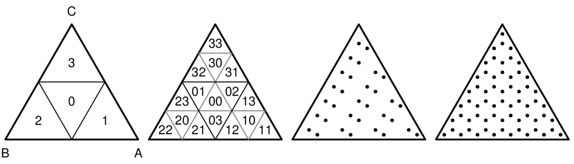
Figure 2: A labeled subdivision of $\Delta(A,B,C)$ into $4$ and then $16$ congruent subtriangles. Next are the first $32$ triangular van der Corput points followed by the first $64$.

We write the integer $i>0$ in a base $4$ representation $i=\sum_{k=1}^{K_{i}}d_{k}4^{k-1}$ where $d_{k}=d_{k}(i)\in\{0,1,2,3\}$ and $K_{i}=\lceil\log_{4}(i)+1\rceil$. Given a triangle $T$, we map the integer $i$ to the point $f_{T}(i)\in T$ as follows. First we identify the subtriangle of $T$ corresponding to $d_{1}$. Call it $T(d_{1})$. Then we get the subtriangle $T(d_{1},d_{2})=(T(d_{1}))(d_{2})$ corresponding to digit $d_{2}$ within $T(d_{1})$, and so on. This process maps the integer $i$ to the triangle $T(d_{1},d_{2},\dots,d_{K_{i}})$. The point $f_{T}(i)$ is the center point of triangle $T(d_{1},d_{2},\dots,d_{K_{i}})$. The center of the triangle is the arithmetic average of its vertices. The triangle $T(d_{1},d_{2},\dots,d_{K_{i}},0,0,\dots,0)$ also has center $f_{T}(i)$, and as we increase the number of zeros beyond $d_{K_{i}}$, the three corners of the resulting triangle all converge to $f_{T}(i)$. For $i=0$, our convention is that $f_{T}(0)$ is the center of the original triangle $T$.

We have not yet formally specified which subtriangle of $T(d_{1})$ we mean by $T(d_{1},d_{2})$ when $d_{2}\neq 0$. To make this precise, let $T=\Delta(A,B,C)$ be an arbitrary triangle. Then for $d\in\{0,1,2,3\}$ the subtriangle of $T$ is

$$T(d)=\begin{cases}\Delta\bigl{(}\frac{B+C}{2},\frac{A+C}{2},\frac{A+B}{2}\bigr{)},&d=0\\[2.15277pt] \Delta\bigl{(}A,\frac{A+B}{2},\frac{A+C}{2}\bigr{)},&d=1\\[2.15277pt] \Delta\bigl{(}\frac{B+A}{2},B,\frac{B+C}{2}\bigr{)},&d=2\\[2.15277pt] \Delta\bigl{(}\frac{C+A}{2},\frac{C+B}{2},C\bigr{)},&d=3.\end{cases}$$

This pattern is followed in Figure 2. If we represent the triangle $T$ by a vector of the three corner points $A$, $B$, and $C$, then $T(1)=(A+T)/2$ componentwise, and similarly $T(2)=(B+T)/2$, $T(3)=(C+T)/2$ and $T(0)=(A+B+C)/2-T/2$.

This construction defines an infinite sequence of $f_{T}(i)\in T$ for integers $i\geqslant 0$. For an $n$ point rule, take $\boldsymbol{x}_{i}=f_{T}(i-1)$ for $i=1,\dots,n$.

This triangular van der Corput sequence has several desirable properties. First, it is extensible. If we have sampled $n$ points and find that we need $m$ more we simply take the next $m$ points in the sequence. Second, it is balanced. If $n=4^{k}$ then we get the centers of a symmetric triangulation as shown by the final panel in Figure 2. If our sample is not a multiple of $4^{k}$, we still have reasonable balance, as illustrated by the third panel in Figure 2. There are $32$ points of which the second $16$ points fall into gaps left by the first $16$ points.

3.1 Discrepancy of triangular van der Corput points

In this subsection, we state and prove some results on the parallel discrepancy of the triangular van der Corput points. That discrepancy is the same for any triangle. We will work with an equilateral triangle ${\Delta_{E}}$ of unit area so that discrepancy calculations reduce to computing areas and counting points. Such a triangle has sides of length $\ell=2/\sqrt[4]{3}$.

Our discussion of these points revolves around a standard decomposition of ${\Delta_{E}}$ into $N=4^{k}$ subtriangles of area $1/N$. These subtriangles are similar to ${\Delta_{E}}$ and have sides parallel to those of ${\Delta_{E}}$. The first two panels in Figure 2 depict such decompositions into $4$ and $16$ subtriangles, respectively. The points $\boldsymbol{x}_{i}=f_{\Delta_{E}}(i-1)$ for $1\leqslant i\leqslant 4^{k}$ are at the centroids of these subtriangles. When we plot ${\Delta_{E}}$ with a horizontal base below its peak, then $2^{k}(2^{k}+1)/2$ of the subtriagles will also be pointing up that way. We call these upright subtriangles. We call the remaining $2^{k}(2^{k}-1)/2$ subtriangles inverted subtriangles.

For our purposes here a line segment ‘touches’ a triangle if it intersects an interior point of that triangle, splitting it into two subsets of positive area.

Theorem 2.

For an integer $k\geqslant 0$ and non-degenerate triangle $\Omega=\Delta(A,B,C)$, let ${\cal P}$ consist of $\boldsymbol{x}_{i}=f_{\Omega}(i-1)$ for $i=1,\dots,N=4^{k}$. Then

$$D_{N}^{\mathrm{P}}({\cal P};\Omega)=\begin{cases}\dfrac{7}{9},&N=1\\[4.30554pt] \dfrac{2}{3\sqrt{N}}-\dfrac{1}{9N},&\text{else.}\end{cases}$$

The proof of Theorem 2 requires consideration of numerous subcases. We defer it to Section 3.2. For $N=1$, the maximal discrepancy is attained by a parallelogram just barely including the center point and holding $2/9$ of the area. It has positive signed discrepancy. For $N=4^{k}>1$, the maximal discrepancy is attained (in the limit) by the trapezoid just barely excluding all $\sqrt{N}$ van der Corput points in the ‘bottom row’ of ${\Delta_{E}}$ and the signed discrepancy is negative. The same limit is also attained in the limit for a sequence of trapezoids having positive signed discrepancy.

Theorem 3.

Let $\Omega$ be a nondegenerate triangle, and let ${\cal P}$ contain points $\boldsymbol{x}_{i}=f_{\Omega}(s+i-1)$, $i=1,\dots,N=4^{k}$, for a starting integer $s\geqslant 1$ and an integer $k\geqslant 0$. Then

$$D_{N}^{\mathrm{P}}({\cal P};\Omega)\leq\frac{2}{\sqrt{N}}-\frac{1}{N}.$$

Proof.

A set $S\in{\cal S}_{C}$ can be written $S={\cal T}_{a,b,C}\cap\Omega$. Let $T_{j}$ be the interiors of the subtriangles of $\Omega$ for $j=1,\dots,N$ and then let $T_{0}=\Omega\,\backslash\cup_{j=1}^{N}T_{j}$. Now define $S_{j}=S\cap T_{j}$, $j=0,1,\dots,N$. Then $\delta_{N}(S)=\sum_{j=0}^{N}\delta_{N}(S_{j})$, from (2). Because the $\boldsymbol{x}_{i}$ are all interior points of their respective subtriangles, we have $\delta_{N}(S_{0})=0$. If the boundary of ${\cal T}_{a,b,C}$ does not touch $S_{j}$ for $1\leqslant j\leqslant N$ then $\delta_{N}(S_{j})=0$ too. Otherwise $-1/N\leqslant\delta_{N}(S_{j})\leqslant 1/N$. Therefore $D_{N}(S;{\cal P})\leqslant m/N$ where $m$ is the number of subtriangles touching a boundary line of ${\cal S}_{a,b,C}$. No such trapezoid can have a boundary touching more than $2\sqrt{N}-1$ subtriangles. Therefore $D_{N}({\cal S}_{C};{\cal P})\leqslant(2\sqrt{N}-1)/N$ and since the same holds for ${\cal S}_{A}$ and ${\cal S}_{B}$, the theorem follows. ∎

Theorem 4.

Let $\Omega$ be a non-degenerate triangle and, for integer $N\geqslant 1$, let ${\cal P}=(\boldsymbol{x}_{1},\dots,\boldsymbol{x}_{N})$, where $\boldsymbol{x}_{i}=f_{\Omega}(i-1)$. Then

$$D_{N}^{\mathrm{P}}({\cal P};\Omega)\leqslant 12/\sqrt{N}.$$

Proof.

Let $N=\sum_{j=0}^{K}a_{j}4^{j}$ for integer $K>0$, with $a_{K}\neq 0$. Let ${\cal P}_{j}^{l}$ denote a set of $4^{j}$ consecutive points from ${\cal P}$, for $l=1,\ldots,a_{j}$ and $j\leqslant K$. These ${\cal P}_{j}^{l}$ can be chosen to partition the $N$ points $\boldsymbol{x}_{i}$. Fix any $S\in{\cal S}_{\mathrm{P}}$. Then,

$$\delta_{N}(S;{\cal P})=\frac{1}{N}\sum_{j=0}^{K}\sum_{l=1}^{a_{j}}4^{j}\delta(S;{\cal P}_{j}^{l}).$$

Therefore from Theorem 2,

$$D_{N}(S;{\cal P})=|\delta_{N}(S;{\cal P})|\leqslant\frac{1}{N}\sum_{j=0}^{K}\sum_{l=1}^{a_{j}}4^{j}\Bigl{(}\frac{2}{2^{j}}-\frac{1}{4^{j}}\Bigr{)}\leqslant\frac{1}{N}\sum_{j=0}^{K}a_{j}(2^{j+1}-1).$$

Because $a_{j}\leqslant 3$,

$$D_{N}(S;{\cal P}) \leqslant\frac{3}{N}\bigl{(}2(2^{K+1}-1)-(K+1)\bigr{)}\leqslant\frac{12\times 2^{K}}{N}$$

and then $K\leqslant\log_{4}(N)$, gives $D_{N}(S;{\cal P})\leqslant{12}/\sqrt{N}$. Taking the supremum over $S\in{\cal S}_{\mathrm{P}}$ yields the result. ∎

Note that this bound can be improved by subtracting a multiple of $\log(N)/N$ but that does not affect the rate.

If we apply the nested uniform digit scrambling of Owen, (1995) to the base $4$ digits of $i-1$, then $\boldsymbol{x}_{i}$ for $i=1,\dots,N=4^{k}$ are independent and uniformly distributed within their subtriangles. In that case, if $f$ has bounded first derivative on ${\Delta_{E}}$ then

$${\mathbb{E}}\Bigl{(}\Bigl{(}\frac{1}{N}\sum_{i=1}^{n}f(\boldsymbol{x}_{i})-\int_{\Delta_{E}}f(\boldsymbol{x})\mathrm{\,d}\boldsymbol{x}\Bigr{)}^{2}\Bigr{)}=O\Bigl{(}\frac{1}{N^{2}}\Bigr{)}$$

because the subtriangles have diameter $O(1/\sqrt{N})$.

3.2 Proof of Theorem 2

The parallel discrepancy is the same for all nondegenerate triangles, so we will work with $\Omega={\Delta_{E}}$. By symmetry of the construction

$$D_{N}^{\mathrm{P}}({\cal P};\Omega)=D_{N}({\cal S}_{A};{\cal P},\Omega)=D_{N}({\cal S}_{B};{\cal P},\Omega)=D_{N}({\cal S}_{C};{\cal P},\Omega),$$

and so it suffices to study $D_{N}({\cal S}_{C};{\cal P},{\Delta_{E}})$.

The sets in ${\cal S}_{C}$ are of the form $S_{a,b}\equiv{\cal T}_{a,b}\cap{\Delta_{E}}$ where $0<a\leqslant\ell$ and $0<b\leqslant\ell$, as depicted in Figure 1. The trapezoid ${\Delta_{E}}=CDFE$ has a horizontal upper boundary line segment $L_{b}\equiv DF$ and a lower slanted boundary line segment $L_{a}\equiv EF$.

The case with $N=1$ can be solved easily. It corresponds to the infimal area of a parallelogram containing the centroid of ${\Delta_{E}}$. From here on we assume $N=4^{k}$ for $k\geqslant 1$.

We will use the decomposition of ${\Delta_{E}}$ into $N=4^{k}$ congruent equilateral subtriangles each of area $1/N$. Of these, there are $2^{k}(2^{k}+1)/2$ upright subtriangles, $2^{k}(2^{k}-1)/2$ inverted triangles and ${\cal P}$ places one point at the centroid of these $4^{k}$ subtriangles.

Recall that a line segment ‘touches’ a triangle if it intersects an interior point of that triangle. We say that the line segment ‘crosses’ a triangle if touches it and also intersects two points on the boundary of the triangle. If neither $L_{a}$ nor $L_{b}$ touch ${\Delta_{E}}$, then $\delta_{N}(S_{a,b};{\cal P})=0$. If $L_{b}$ touches ${\Delta_{E}}$ and $L_{a}$ does not, then $S_{a,b}$ is the subset of ${\Delta_{E}}$ below a horizontal line and we easily find that the greatest discrepancy for this case is

$$\sup_{0\leqslant b<\ell}D_{N}(S_{\ell,b})=\dfrac{2}{3\sqrt{N}}-\dfrac{1}{9N}$$ (7)

attained when $L_{b}$ passes just below the centroids of the bottom row of upright triangles. Such a line contains $0$ points of ${\cal P}$ and its volume is given by (7). By symmetry $\sup_{0\leqslant a<\ell}D_{N}(S_{a,\ell})$ takes the same value.

It remains to consider the case where both $L_{a}$ and $L_{b}$ touch ${\Delta_{E}}$. In this case, to maximize discrepancy, the horizontal line $L_{b}$ must either pass just above a row of upright subtriangle’s centroids, just below such a row, or just above or below a row of inverted subtriangle’s centroids. Similarly the slanted line $L_{a}$ must pass just left or just right of a slanted row of centroids, or else discrepancy can be increased.

There are 4 cases. The intersection of $L_{a}$ and $L_{b}$ could be inside an upright subtriangle, inside an inverted subtriangle, outside of ${\Delta_{E}}$ touching two disjoint bands of subtriangles, or outside of ${\Delta_{E}}$ touching two bands of one or more subtriangles that share an upright subtriangle. These cases are illustrated in Figure 3.

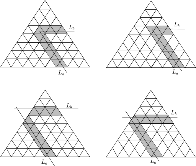
Figure 3: This figure illustrates the four cases that can arise when both $L_{a}$ and $L_{b}$ touch ${\Delta_{E}}$.

As in Theorem 4, the signed discrepancy $\delta_{N}(\cdot)$ can be summed over the subtriangles. The cases in Figure 3 include subtriangles touched by $0$, $1$ or $2$ of the boundary lines. A subtriangle touched by $0$ boundary lines does not contribute to the discrepancy.

Suppose that the upright subtriangle $T$ is crossed by one horizontal line passing just above the centroid of an inverted triangle to the left or right of $T$. Referring to Figure 4 we see that $8/9$ of the area of that upright triangle is below the line as is its one point. As a result, the signed discrepancy contribution $\delta_{N}(\cdot)$ for that subtriangle is $1-8/9=1/9$ of the area of this triangle, that is $1/(9N)$. Similarly, the portion of an inverted subtriangle below that line has $4/9$ of the area and also the one and only point, for a signed discrepancy contribution of $5/(9N)$. These two facts are recorded in the first row of Table 1. The three other relevant horizontal lines are also summarized in Table 1.

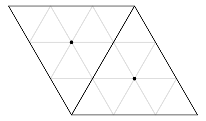
Figure 4: This figure shows a trapezoid made up of one upright subtriangle and one inverted subtriangle. Each subtriangle has area $1/N$ and contains $1$ point of ${\cal P}$ at its centroid, as shown.

	Upright			Inverted			Total
Horiz. Line	pts	vol	$\delta_{u}$	pts	vol	$\delta_{i}$	$\delta_{u}+\delta_{i}$
Inv $+$	$1$	$8/9$	$\phantom{-}1/9$	$1$	$4/9$	$\phantom{-}5/9$	$\phantom{-}2/3$
Inv $-$	$1$	$8/9$	$\phantom{-}1/9$	$0$	$4/9$	$-4/9$	$-1/3$
Upr $+$	$1$	$5/9$	$\phantom{-}4/9$	$0$	$1/9$	$-1/9$	$\phantom{-}1/3$
Upr $-$	$0$	$5/9$	$-5/9$	$0$	$1/9$	$-1/9$	$-2/3$

Table 1: Signed discrepancies for subtriangles crossed horizontally by $L_{b}$ and not touched by $L_{a}$. Line Inv$+$ passes just above the centroid of the inverted subtriangle, Inv$-$ passes just below it. Upr$\pm$ are similarly defined with respect to the centroid of the upright subtriangle. For each subtriangle we record the number of centroid points and the fraction of its volume below each line as well as $N$ times the signed discrepancy contribution of that subtriangle and the total signed discrepancy of the trapezoid they form.

Also in that table, we see the total discrepancy of two triangles, one upright and one inverted, when they are both crossed by the same horizontal line. These subtrapezoids play an important role in the analysis. The signed discrepancy contribution of a subtrapezoid can be has high as $2/(3N)$ when the line crosses just above the centroid of the inverted triangle, and as low as $-2/(3N)$ when it passes just below the centroid of the upright triangle. The same discrepancies hold for triangles crossed by the slanted line $L_{a}$ intersecting the base of ${\Delta_{E}}$ at distance $a$ from $C$, where as before $\pm$ indicates values of $a$ just barely including/excluding a subtriangle’s centroid.

Now consider a subtriangle touched by both lines $L_{a}$ and $L_{b}$. We can see from Figure 4 that if an inverted subtriangle is touched by both lines then they must have met at its centroid. The signed discrepancy from that triangle is then $8/(9N)$ if both lines included the centroid and $-1/(9N)$ if either excluded it.

	Slanted line $L_{a}$
Horiz. Line	Inv$+$	Inv$-$	Up$+$	Up$-$	Right Trap.
Inv$+$	$\phantom{-}\dfrac{2}{9N}$	$\phantom{-}\dfrac{2}{9N}$	$\phantom{-}\dfrac{5}{9N}$	$-\dfrac{4}{9N}$	$\dfrac{2}{3N}$
Inv$-$	$\phantom{-}\dfrac{2}{9N}$	$\phantom{-}\dfrac{2}{9N}$	$\phantom{-}\dfrac{5}{9N}$	$-\dfrac{4}{9N}$	$-\dfrac{1}{3N}$
Upr$+$	$\phantom{-}\dfrac{5}{9N}$	$\phantom{-}\dfrac{5}{9N}$	$\phantom{-}\dfrac{7}{9N}$	$-\dfrac{2}{9N}$	$\dfrac{1}{3N}$
Upr$-$	$-\dfrac{4}{9N}$	$-\dfrac{4}{9N}$	$-\dfrac{2}{9N}$	$-\dfrac{2}{9N}$	$-\dfrac{2}{3N}$
Lower Trap.	$\dfrac{2}{3N}$	$-\dfrac{1}{3N}$	$\dfrac{1}{3N}$	$-\dfrac{2}{3N}$

Table 2: Signed discrepancies for an upright subtriangle $T$ touched by $L_{a}$ and $L_{b}$. Rows designate $4$ relevant horizontal lines, columns the slanted lines. The main table shows the signed discrepancy of $T$. The rightmost column shows the signed discrepancy of trapezoids to the right of $T$. The bottom row shows the signed discrepancy of trapezoids below $T$.

If both boundary lines touch an upright subtriangle $T$ those lines can meet just above or just below $T$’s centroid, or they can meet just above or just below the centroid of an inverted subtriangle to the left of $T$. Table 2 enumerates the cases along with their signed discrepancies, the signed discrepancies of any trapezoids to the right of $T$, and the signed discrepancies of trapezoids below (and right) of $T$.

Now we consider our four cases. First, if $L_{a}\cap L_{b}$ is in an upright subtriangle $T$ then $T$ is the only subtriangle touched by two lines. The total signed discrepancy is that from within $T$ together with as many as $\sqrt{N}-1$ trapezoids. For $N=1$ there were none of these trapezoids, but for $N\geqslant 4$, at least $3$ trapezoids can contribute. Referring to Table 2, we see that maximizing the contribution from trapezoids will maximize the discrepancy irrespective of the signed discrepancy from $T$. We maximize discrepancy by finding the largest possible $|\delta_{N}(T)|$ for which either the trapezoids in its row or column have $\delta_{N}=\pm 2/(3N)$ with a sign matching $\delta_{N}(T)$. The result using $\sqrt{N}-1$ such trapezoids gives discrepancy

$$\delta_{N}(S_{a,b})=\frac{5}{9N}+(\sqrt{N}-1)\frac{2}{3N}=\frac{2}{3\sqrt{N}}-\frac{1}{9N},$$

tying the discrepancy (7) from the large empty region below all the $\boldsymbol{x}_{i}$.

The second case has $L_{a}\cap L_{b}$ in an inverted subtriangle. There is always an upright subtriangle to the right of an inverted one, both of those subtriangles are touched by $L_{a}$ and $L_{b}$, and no others are touched by two of these lines. The inverted triangle has signed discrepancy $-1/(9N)$ or $8/(9N)$ and the upright triangle to its right has signed discrepancy $2/(9N)$ for a total of $1/(9N)$ or $10/(9N)$. There can be as many as $\sqrt{N}-2$ parallelogram pairs contributing to the total discrepancy which cannot therefore exceed

$$\frac{10}{9N}+(\sqrt{N}-2)\frac{2}{3N}=\frac{2}{3\sqrt{N}}-\frac{2}{9N}.$$

As a result, the second case cannot maximize discrepancy.

The third case has $L_{a}$ and $L_{b}$ intersecting outside ${\Delta_{E}}$ and touching two bands of parallelograms that intersect in one upright triangle $T$. The greatest possible discrepancy here arises from $\sqrt{N}-1$ trapezoids and one upright triangle. This is the same configuration as in case 1 and hence cannot exceed (7) either.

The fourth and final case has $L_{a}$ and $L_{b}$ touching two bands of parallelograms that don’t intersect. As a result there are at most $\sqrt{N}-2$ parallelograms contributing to the discrepancy along with $2$ upright triangles touched by one line each. The greatest absolute discrepancy attainable this way is thus

$$(\sqrt{N}-2)\frac{2}{3N}+2\times\frac{4}{9N}=\frac{2}{3\sqrt{N}}-\frac{4}{9N}.$$

Having exhausted the cases, we conclude that for $N=4^{k}>1$, $D_{N}^{\mathrm{P}}({\cal P})=(2/3\sqrt{N})-1/(9N)$. $\Box$

4 Triangular Kronecker Lattices

In this section we use Theorem 1 of Chen and Travaglini, (2007) to construct points in the triangle with a parallel discrepancy of $O({\log(N)}/{N})$. The construction is through a suitably scaled copy of the lattice $\mathbb{Z}^{2}$ rotated through an angle. The chosen angle makes tangents of certain angles badly approximable in the same way that Kronecker sequences use badly approximable numbers for sampling of the unit cube (Larcher and Niederreiter,, 1993). We begin with some definitions.

Definition 1.

A real number $\theta$ is said to be badly approximable if there exists a constant $c>0$ such that $n||n\theta||>c$ for every natural number $n\in\mathbb{N}$ and $||\cdot||$ denotes the distance from the nearest integer.

Definition 2.

Let $a$, $b$, $c$ and $d$ be integers with $b\neq 0$, $d\neq 0$ and $c>0$, where $c$ is not a perfect square. Then $\theta=(a+b\sqrt{c})/d$ is a quadratic irrational number.

Quadratic irrational numbers have a periodic repeating continued fraction representation, and they are badly approximable (Hensley,, 2006).

Let $\Theta=\{\theta_{1},\dots,\theta_{k}\}$ be a set of $k\geqslant 1$ angles in $[0,2\pi)$. Then let ${\cal A}(\Theta)$ be the set of convex polygonal subsets of $[0,1]^{2}$ whose sides make an angle of $\theta_{i}$ with respect to the horizontal axis. Theorem 1 of Chen and Travaglini, (2007) says that there exists a constant $C_{\Theta}<\infty$ such that for any integer $N>1$ there exists a list ${\cal P}=(\boldsymbol{x}_{1},\dots,\boldsymbol{x}_{N})$ of points in $[0,1]^{2}$ with

$$D_{N}({\cal A}(\Theta);{\cal P},[0,1]^{2})<C_{\Theta}\log(N)/N.$$ (8)

Their proof of Theorem 1 relies on this lemma:

Lemma 2.

Suppose that the angles $\theta_{1},\dots,\theta_{k}\in[0,2\pi)$ are fixed. Then there exists $\alpha\in[0,2\pi)$ such that $\tan(\alpha),\tan(\alpha-\pi/2),\tan(\alpha-\theta_{1}),\dots\tan(\alpha-\theta_{k})$ are all finite and badly approximable.

Proof.

This is Lemma 2.2 of Chen and Travaglini, (2007). ∎

Given an $\alpha$ as described by Lemma 2, they construct a list of $N$ points in $[0,1]^{2}$ satisfying (8). To obtain their points they take the lattice $N^{-1/2}\mathbb{Z}^{2}$ and rotate it through an angle $\alpha$ anticlockwise about the origin, and retain only those points which lie in $[0,1]^{2}$. The result will not necessarily have $N$ points, but by adding or removing $O(\log(N))$ points they arrive at a set ${\cal P}$ of $N$ points in $[0,1]^{2}$.

To apply their method, we will place points inside the right angle triangle

$$R=\Delta((0,0)^{\mathsf{T}},(0,1)^{\mathsf{T}},(1,0)^{\mathsf{T}}).$$ (9)

The sides of the parallelograms of the form ${\cal T}_{a,b,C}$, ${\cal T}_{a,c,B}$ and ${\cal T}_{b,c,A}$ for triangle $R$ make angles $0$, $\pi/2$ and $3\pi/4$ (and no others) with respect to the horizontal axis. Intersecting any of those parallelograms with $R$ always yields a convex polygon whose sides make an angle of $0$, $\pi/2$ or $3\pi/4$ with the horizontal axis. Lemma 3 supplies for this set of angles some choices for the $\alpha$ whose existence is asserted by Lemma 2.

Lemma 3.

Let $\alpha$ be an angle for which $\tan(\alpha)$ is a quadratic irrational number. Then $\tan(\alpha)$, $\tan(\alpha-\pi/2)$ and $\tan(\alpha-3\pi/4)$ are all finite and badly approximable.

Proof.

Write $\tan(\alpha)=(a+b\sqrt{c})/d$ for integers $a$, $b$, $c$ and $d$ satisfying $b\neq 0$, $d\neq 0$, and $c>0$, with $c$ not the square of an integer. First, $\tan(\alpha)$ is badly approximable (and finite) because it is quadratic irrational. Similarly,

$$\tan(\alpha-\pi/2)=-\cot(\alpha)=\frac{d}{a+b\sqrt{c}}=\frac{da-bd\sqrt{c}}{a^{2}-b^{2}c}$$

is finite and badly approximable. Note that the denominator in $\tan(\alpha-\pi/2)$ is not zero because $c$ is not a perfect square, and $bd\neq 0$ too. Finally,

$$\tan(\alpha-3\pi/4)=\frac{1+\tan(\alpha)}{1-\tan(\alpha)}=\frac{1+\frac{a+b\sqrt{c}}{d}}{1-\frac{a+b\sqrt{c}}{d}}=\frac{(d-a)^{2}+b^{2}c+2bd\sqrt{c}}{(d-a)^{2}-b^{2}c}$$

is also finite and badly approximable. ∎

As an example, $\tan(3\pi/8)=1+\sqrt{2}$ is a quadratic irrational. Therefore the angle $\alpha=3\pi/8$ satisfies the conditions of Lemma 3.

Theorem 5.

Let $N>1$ be an integer and let $R$ be the triangle given by (9). Let $\alpha\in(0,2\pi)$ be an angle for which $\tan(\alpha)$ is a quadratic irrational. Let ${\cal P}_{1}$ be the points of the lattice $(2N)^{-1/2}\mathbb{Z}^{2}$ rotated anticlockwise by angle $\alpha$. Let ${\cal P}_{2}$ be the points of ${\cal P}_{1}$ that lie in $R$. If ${\cal P}_{2}$ has more than $N$ points, let ${\cal P}_{3}$ be any $N$ points from ${\cal P}_{2}$, or if ${\cal P}_{2}$ has fewer than $N$ points, let ${\cal P}_{3}$ be a list of $N$ points in $R$ including all those of ${\cal P}_{2}$. Then there is a constant $C$ with

$$D^{\mathrm{P}}({\cal P}_{3};R)<C\log(N)/N.$$

Proof.

By Lemma 3, the angle $\alpha$ in the hypothesis of this theorem satisfies the conditions required by the construction of Chen and Travaglini, (2007). We may therefore use that construction to get $2N$ points ${\cal P}_{1}$ in $[0,1]^{2}$ such that their Theorem 1 yields $D_{2N}({\cal P}_{1};{\cal A}(\Theta))<C_{\Theta}\log(2N)/(2N)$ where $\Theta=\{0,\pi/2,3\pi/4\}$. Because the set $R\in{\cal A}(\Theta)$ and has area $1/2$, we know that the number of points in ${\cal P}_{2}$ is between $N-C_{\Theta}\log(2N)/(2N)$ and $N+C_{\Theta}\log(2N)/(2N)$. Then ${\cal P}_{3}$ and ${\cal P}_{2}$ differ by at most $C_{\Theta}\log(2N)/(2N)$ points, so that

$$D^{\mathrm{P}}({\cal P}_{3},R)<2C_{\Theta}\log(2N)/(2N)=C_{\Theta}\log(2N)/N,$$

and we may take $C=2C_{\Theta}$. ∎

Because $D^{\mathrm{P}}$ is invariant under linear mappings, we may then map the points ${\cal P}_{3}$ of $R$ linearly onto any triangle we desire to sample, and attain the same discrepancy. We note that Chen and Travaglini, (2007) analyze their procedure in a different way from how they define it. To simplify notation, they scale the unit square up to $U_{N}=[0,\sqrt{N}]^{2}$ and then rotate $U_{N}$ through an angle of $-\alpha$, and bound the discrepancy of the corresponding scaled and rotated polygons. The resulting discrepancy bounds apply either way.

Our lattice algorithm runs as follows. Given a target sample size $N$, an angle $\alpha$ such as $3\pi/8$ satisfying Lemma 3, and a target triangle $\Delta(A,B,C)$,

1. $n\leftarrow\lceil\sqrt{2N}\rceil+1$

2. ${\cal P}\leftarrow\{-n,-n+1,\dots,n-1,n\}^{2}$

3. For each $\boldsymbol{x}_{i}$ in ${\cal P}$, $\boldsymbol{x}_{i}\leftarrow\bigl{(}\begin{smallmatrix}\cos(\alpha)&-\sin(\alpha)\\ \sin(\alpha)&\phantom{-}\cos(\alpha)\end{smallmatrix}\bigr{)}{\boldsymbol{x}_{i}}/{\sqrt{2N}}$

4. Remove points from ${\cal P}$ that are not in $R$

5. (Optional) add points to or remove points from ${\cal P}$ to get $N$ points in $R$

6. Linearly map ${\cal P}$ from $R$ to $\Delta(A,B,C)$: $A+(C-A)x_{i1}+(B-A)x_{i2}$.

Steps $1$ and $2$ generate a subset of $\mathbb{Z}^{2}$ containing all the points that might possibly end up in $R$ after rotation. Step $3$ does the rotation. Step 4 retains those rotated points that lie in $R$. Step 5 is optional; in applications it may not be important to get precisely $N$ points in $\Delta(A,B,C)$. For $\boldsymbol{x}_{i}=(x_{i1},x_{i2})^{\mathsf{T}}$, Step 6 maps $(0,0)^{\mathsf{T}}$ onto $A$, $(0,1)^{\mathsf{T}}$ onto $B$ and $(1,0)^{\mathsf{T}}$ onto $C$.

Figure 5 shows some points contructed this way. Two of the examples use angles with badly approximable tangents and the other two do not. Those latter ones leave some relatively large trapezoids nearly empty.

Figure 5: Triangular lattice points for target $N=64$. Domain is an equilateral triangle. Angles $3\pi/8$ and $5\pi/8$ have badly approximable tangents. Angles $\pi/4$ and $\pi/2$ have integer and infinite tangents respectively and do not satisfy the conditions for discrepancy $O(\log(N)/N)$.

Figure 6 plots the parallelogram discrepancy for angle $\alpha=3\pi/8$. We see that already for $N$ in the range $10$ to $500$ the discrepancy runs roughly parallel to the asymptotic bound $O(\log(N)/N)$. Results from Beck and Chen, (1987) (cited in Chen and Travaglini, (2007)) show that $D^{\mathrm{P}}_{N}({\cal P})$ cannot be $o(\log(N)/N)$.

Figure 6: Parallel discrepancy of triangular lattice points for angle $\alpha=3\pi/8$ and various targets $N$. The number of points was always $N$ or $N+1$. The dashed reference line is $1/N$. The solid line is $\log(N)/N$.

We may want to randomly shift the points. This can be done by adding a vector $\boldsymbol{U}\sim\mathbf{U}(-1/2,1/2)^{2}$ to each point in ${\cal P}$ at step 2. There are two benefits to randomly shifting the points. First, with probability one there will be no point rotated exactly on the boundary of $R$, and we can then use simple averaging instead of dividing the weighted sum (6) by $N$. The second advantage is that can use independent repetitions of this randomization to estimate error.

5 Riemann integrable functions

The usual definition of Riemann Integral of a bounded function on a set in $\mathbb{R}^{2}$ can be found many books on, such as Ash and Doléans-Dade, (2000) or Marsden, (1974). Here we develop an analogue for the triangle.

Let $T$ be nondegenerate closed triangle in ². For $k\geqslant 0$ and $N=4^{k}$, let $T_{k,1},\dots,T_{k,N}$ be the partition of $T$ into $N$ congruent triangles, similar to $T$. Let $f$ be a bounded function on $T$. We say that $f$ is Riemann integrable on $T$ if

$$\lim_{k\to\infty}\frac{1}{4^{k}}\sum_{i=1}^{4^{k}}f(\boldsymbol{x}_{k,i})=\mu\in\real$$

exists for any choices of $\boldsymbol{x}_{k,i}\in T_{k,i}$. Then we take $\int_{T}f(\boldsymbol{x})\mathrm{\,d}\boldsymbol{x}=\mu\times{\mathbf{vol}}(T)$.

For $k\geqslant 1$ and $i=1,\dots,4^{k}$, let

$$\begin{split}m_{k,i}=\inf\{f(\boldsymbol{x})\mid\boldsymbol{x}\in T_{k,i}\}\quad\text{and}\quad M_{k,i}=\sup\{f(\boldsymbol{x})\mid\boldsymbol{x}\in T_{k,i}\}.\end{split}$$

Then $f$ is Riemann integrable if and only if $\lim_{k\to\infty}\sum_{i=1}^{4^{k}}(M_{k,i}-m_{k,i})/4^{k}=0.$ By modifying an argument in (Ash and Doléans-Dade,, 2000, Theorem 1.6.6), $f$ is Riemann integrable if it is bounded and continuous almost everywhere on $T$. When the Riemann integral exists, it matches the Lebesgue integral.

Figure 7: Figure to illustrate decomposition of signed discrepancies of upright (respectively inverted) subtriangle $A$ in terms of parallelograms.

Lemma 4.

Let $T$ be a triangle and ${\cal P}$ a list of $N\geqslant 1$ points in $T$, having parallel discrepancy $D^{\mathrm{P}}_{N}({\cal P};T)$. Let $S$ be a subtriangle of $T$ with sides parallel to those of $T$. Then $D_{N}(S;{\cal P})\leqslant 6D^{\mathrm{P}}_{N}({\cal P};T)$.

Proof.

First suppose that $S$ is inverted with respect to $T$ shown as $A$ in the left panel of Figure 7. Let the subsets $A$, $B$, $\dots$, $F$ indicated there be disjoint, and have union $T$. Let $AB$, $ABDF$ et cetera be unions of those sets. Then with the signed discrepancy function $\delta(\cdot)=\delta_{N}(\cdot;{\cal P},T)$, and these six sets in ${\cal S}_{\mathrm{P}}$,

$$\phantom{=}\ \delta(AB)+\delta(AC)+\delta(AD)-\delta(ABDF)-\delta(ACDE)-\delta(ACGB)$$

$$=-\delta(B)-\delta(C)-\delta(D)-\delta(E)-\delta(F)-\delta(G)$$

$$=\delta(A),$$

using additivity of signed discrepancy, and $\delta(ABCDEFG)=\delta(T)=0$. Next let $S$ be the upright triangle shown as $A$ in the right panel of Figure 7. Then using $6$ sets from ${\cal S}_{\mathrm{P}}$,

$$\phantom{=}\ \delta(ABFG)+\delta(ADEF)+\delta(ACEG)+\delta(B)+\delta(C)+\delta(D)$$

$$=3\delta(A)+2\delta(B)+2\delta(C)+2\delta(D)+2\delta(E)+2\delta(F)+2\delta(G)$$

$$=\delta(A).$$

In either case, $|\delta(A)|\leqslant 6D^{\mathrm{P}}_{N}({\cal P};T)$, and so $D_{N}(S;{\cal P})\leqslant 6D_{N}^{\mathrm{P}}({\cal P};T)$. ∎

Theorem 6.

Let $f$ be a Riemann integrable function on a nondegenerate triangle $\Omega$, and let ${\cal P}_{N}=(\boldsymbol{x}_{N,1},\boldsymbol{x}_{N,2},\dots,\boldsymbol{x}_{N,N})$ for $\boldsymbol{x}_{N,i}\in\Omega$. If $\lim_{N\to\infty}D^{\mathrm{P}}_{N}({\cal P};\Omega)=0$, then

$$\lim_{N\to\infty}\frac{{\mathbf{vol}}(\Omega)}{N}\sum_{i=1}^{N}f(\boldsymbol{x}_{N,i})=\int_{\Omega}f(\boldsymbol{x})\mathrm{\,d}\boldsymbol{x}.$$

Proof.

Fix $\epsilon>0$ and then choose $k\geqslant 0$ so that $4^{-k}\sum_{i=1}^{4^{k}}(M_{k,i}-m_{k,i})<\epsilon$. Let $T_{1},\dots,T_{4^{k}}$ be the $4^{k}$ congruent subtriangles of $\Omega$. Then

$$\frac{{\mathbf{vol}}(\Omega)}{N}\sum_{i=1}^{N}f(\boldsymbol{x}_{N,i}) =\sum_{j=1}^{4^{k}}\frac{{\mathbf{vol}}(\Omega)}{N}\sum_{i=1}^{N}1_{\boldsymbol{x}_{N,i}\in T_{j}}f(\boldsymbol{x}_{N,i})$$

$$\leqslant\sum_{j=1}^{4^{k}}\frac{{\mathbf{vol}}(\Omega)}{N}\sum_{i=1}^{N}1_{\boldsymbol{x}_{N,i}\in T_{j}}M_{k,j}$$

$$={\mathbf{vol}}(\Omega)\sum_{j=1}^{4^{k}}\bigl{(}4^{-k}+\delta_{N}(T_{j};{\cal P}_{N})\bigr{)}M_{k,j}.$$

From Lemma 4, $|\delta_{N}(T_{j};{\cal P}_{N})|\leqslant 6D_{N}^{\mathrm{P}}({\cal P}_{N})$. Therefore

$$\frac{{\mathbf{vol}}(\Omega)}{N}\sum_{i=1}^{N}f(\boldsymbol{x}_{N,i})\leqslant\int_{\Omega}f(\boldsymbol{x})\mathrm{\,d}\boldsymbol{x}+\epsilon{\mathbf{vol}}(\Omega)+6\times 4^{k}D_{N}^{\mathrm{P}}({\cal P}_{N}){\mathbf{vol}}(\Omega)|M_{0,1}|.$$

Similarly,

$$\frac{{\mathbf{vol}}(\Omega)}{N}\sum_{i=1}^{N}f(\boldsymbol{x}_{N,i})\geqslant\int_{\Omega}f(\boldsymbol{x})\mathrm{\,d}\boldsymbol{x}-\epsilon{\mathbf{vol}}(\Omega)-6\times 4^{k}D_{N}^{\mathrm{P}}({\cal P}_{N}){\mathbf{vol}}(\Omega)|m_{0,1}|.$$

To complete the proof, let $N\to\infty$ and then note that $\epsilon$ was arbitrary. ∎

6 Discussion

The Kronecker construction attains a lower discrepancy than the van der Corput construction. But the van der Corput construction is extensible and the digits in it can be randomized. If the integrand $f$ is continuously differentiable, then for $N=4^{k}$, the randomization in Owen, (1995) will produce integral estimates with a root mean squared error $O(N^{-1})$, slightly better than the Koksma-Hlawka bound for the deterministic Kronecker construction. As a result, we anticipate that both constructions will be useful in applications. The variation measure used by Brandolini et al., (2013) requires even more smoothness than one derivative and so

Spherical triangles are also of interest. The digital construction can be used to generate points inside a proper spherical triangle (all angles less than $\pi$) with corners $A$, $B$ and $C$ if averages like $(A+B)/2$ are projected back to the surface of the sphere, to get the midpoint of the arc from $A$ to $B$.

References

- Aistleitner et al., (2012) Aistleitner, C., Brauchart, J. S., and Dick, J. (2012). Point sets on the sphere with small spherical cap discrepancy. Discrete & Computational Geometry, 48(4):990–1024.
- Arvo, (1995) Arvo, J. (1995). Stratified sampling of spherical triangles. In Proceedings of the 22nd annual conference on Computer graphics and interactive techniques, pages 437–438. ACM.
- Ash and Doléans-Dade, (2000) Ash, R. B. and Doléans-Dade, C. (2000). Probability and measure theory. Harcourt, San Diego, CA, second edition.
- Beck and Chen, (1987) Beck, J. and Chen, W. W. L. (1987). Irregularities of Distribution. Cambridge University Press, New York.
- Brandolini et al., (2013) Brandolini, L., Colzani, L., Gigante, G., and Travaglini, G. (2013). A Koksma–Hlawka inequality for simplices. In Trends in Harmonic Analysis, pages 33–46. Springer.
- Chen and Travaglini, (2007) Chen, W. W. L. and Travaglini, G. (2007). Discrepancy with respect to convex polygons. Journal of Complexity, 23(4–6):662–672. Festschrift for the 60th Birthday of Henryk Woźniakowski.
- Devroye, (1986) Devroye, L. (1986). Non-uniform Random Variate Generation. Springer.
- Fang and Wang, (1994) Fang, K.-T. and Wang, Y. (1994). Number Theoretic Methods in Statistics. Chapman & Hall.
- Hensley, (2006) Hensley, D. (2006). Continued fractions. World Scientific, Singapore.
- Larcher and Niederreiter, (1993) Larcher, G. and Niederreiter, H. (1993). Kronecker-type sequences and non-Archimedean Diophantine approximations. Acta Arithmetica, 63(4):379–396.
- Lyness and Cools, (1994) Lyness, J. N. and Cools, R. (1994). A survey of numerical cubature over triangles. In Proceedings of Symposia in Applied Mathematics, volume 48, pages 127–150.
- Marsden, (1974) Marsden, J. (1974). Elementary classical analysis. W. H. Freeman and Company, San Francisco.
- Niederreiter, (1992) Niederreiter, H. (1992). Random Number Generation and Quasi-Monte Carlo Methods. S.I.A.M., Philadelphia, PA.
- Owen, (1995) Owen, A. B. (1995). Randomly permuted -nets and -sequences. In Niederreiter, H. and Shiue, P. J.-S., editors, Monte Carlo and Quasi-Monte Carlo Methods in Scientific Computing, pages 299–317, New York. Springer-Verlag.
- Owen, (2005) Owen, A. B. (2005). Multidimensional variation for quasi-Monte Carlo. In Fan, J. and Li, G., editors, International Conference on Statistics in honour of Professor Kai-Tai Fang’s 65th birthday.