Functional A Posteriori Error Equalities
for Conforming Mixed Approximations
of Elliptic Problems

Immanuel Anjam111Department of Mathematical Information Technology, University of Jyväskylä, P.O. Box 35 (Agora), FI-40014 University of Jyväskylä, Finland, email: immanuel.anjam@jyu.fi  & Dirk Pauly222Fakultät für Mathematik, Universität Duisburg-Essen, Campus Essen, Thea-Leymann-Str. 9, DE-45141 Essen, Germany, email: dirk.pauly@uni-due.de

Dedicated to Sergey Igorevich Repin on the occasion of his 60thsuperscript60th60^{\textrm{th}} birthday

Abstract  In this paper we show how to find the exact error (not just an estimate of the error) of a conforming mixed approximation by using the functional type a posteriori error estimates in the spirit of Repin [14]. The error is measured in a mixed norm which takes into account both the primal and dual variables. We derive this result for all elliptic partial differential equations of the class

AAx+x=f,superscriptAA𝑥𝑥𝑓\operatorname{A}^{*}\operatorname{A}\,x+x=f,

where AA\operatorname{A} is a linear, densely defined and closed (usually a differential) operator and AsuperscriptA\operatorname{A}^{*} its adjoint. We first derive a special version of our main result by using a simplified reaction-diffusion problem to demonstrate the strong connection to the classical functional a posteriori error estimates of Repin [14]. After this we derive the main result in an abstract setting. Our main result states that in order to obtain the exact global error value of a conforming mixed approximation with primal variable x𝑥x and dual variable y𝑦y, i.e.,

Ay+x=f,Ax=y,formulae-sequencesuperscriptA𝑦𝑥𝑓A𝑥𝑦\operatorname{A}^{*}y+x=f,\quad\operatorname{A}x=y,

one only needs the problem data and the mixed approximation (x~,y~)D(A)×D(A)~𝑥~𝑦𝐷A𝐷superscriptA(\tilde{x},\tilde{y})\in D(\operatorname{A})\times D(\operatorname{A}^{*}) of the exact solution (x,y)D(A)×(D(A)R(A))𝑥𝑦𝐷A𝐷superscriptA𝑅A(x,y)\in D(\operatorname{A})\times\big{(}D(\operatorname{A}^{*})\cap R(\operatorname{A})\big{)}, i.e., the equality

|xx~|2+|A(xx~)|2+|yy~|2+|A(yy~)|2=|fx~Ay~|2+|y~Ax~|2superscript𝑥~𝑥2superscriptA𝑥~𝑥2superscript𝑦~𝑦2superscriptsuperscriptA𝑦~𝑦2superscript𝑓~𝑥superscriptA~𝑦2superscript~𝑦A~𝑥2|x-\tilde{x}|^{2}+|\operatorname{A}(x-\tilde{x})|^{2}+|y-\tilde{y}|^{2}+|\operatorname{A}^{*}(y-\tilde{y})|^{2}=|f-\tilde{x}-\operatorname{A}^{*}\tilde{y}|^{2}+|\tilde{y}-\operatorname{A}\tilde{x}|^{2}

holds. There is no need for calculating any auxiliary data. The calculation of the exact error consists of simply calculating two (usually integral) quantities where all the quantities are known after the approximate solution has been obtained by any conforming method guaranteeing (x~,y~)D(A)×D(A)~𝑥~𝑦𝐷A𝐷superscriptA(\tilde{x},\tilde{y})\in D(\operatorname{A})\times D(\operatorname{A}^{*}). We also show some numerical computations to confirm the results.

Key words  functional a posteriori error estimate, error equality, elliptic boundary value problem, mixed formulation, combined norm

AMS MSC-Classifications  65N15

1 Introduction

The results presented in this paper are based on the conception of functional type a posteriori error estimates. These type estimates are valid for any conforming approximation and contain only global constants. We note that estimates for nonconforming approximations are known as well but will not be discussed in this paper. In the case of the class of PDEs studied in this paper, the estimates do not contain even global constants. For a detailed exposition of the theory see the books [14] by Repin and [9] by Repin and Neittaanmäki or for a more computational point of view [8] by Mali, Repin, and Neittaanmäki.

We will measure the error of our approximations in a combined norm, which includes the error of both, the primal and the dual variable. This is especially useful for mixed methods where one calculates an approximation for both the primal and dual variables, see e.g. the book of Brezzi and Fortin [2].

In this paper, we study the linear equation

(Aα2A+α1)x=fsuperscriptAsubscript𝛼2Asubscript𝛼1𝑥𝑓(\operatorname{A}^{*}\alpha_{2}\operatorname{A}+\alpha_{1})x=f

presented in the mixed form

Ay+α1x=f,α2A=y,formulae-sequencesuperscriptA𝑦subscript𝛼1𝑥𝑓subscript𝛼2A𝑦\operatorname{A}^{*}y+\alpha_{1}x=f,\quad\alpha_{2}\operatorname{A}=y,

where α1,α2subscript𝛼1subscript𝛼2\alpha_{1},\alpha_{2} are linear and self adjoint topological isomorphisms on two Hilbert spaces 𝖧1subscript𝖧1\operatorname{\sf H}_{1} and 𝖧2subscript𝖧2\operatorname{\sf H}_{2} and A:D(A)𝖧1𝖧2:A𝐷Asubscript𝖧1subscript𝖧2\operatorname{A}:D(\operatorname{A})\subset\operatorname{\sf H}_{1}\to\operatorname{\sf H}_{2} is a linear, densely defined and closed operator with adjoint operator A:D(A)𝖧2𝖧1:superscriptA𝐷superscriptAsubscript𝖧2subscript𝖧1\operatorname{A}^{*}:D(\operatorname{A}^{*})\subset\operatorname{\sf H}_{2}\to\operatorname{\sf H}_{1}. Our main result is Theorem 3.4 and it shortly reads as the functional a posterior error equality

|xx~|𝖧1,α12+|A(xx~)|𝖧2,α22+|yy~|𝖧2,α212+|A(yy~)|𝖧1,α112=|fα1x~Ay~|𝖧1,α112+|y~α2Ax~|𝖧2,α212superscriptsubscript𝑥~𝑥subscript𝖧1subscript𝛼12superscriptsubscriptA𝑥~𝑥subscript𝖧2subscript𝛼22superscriptsubscript𝑦~𝑦subscript𝖧2superscriptsubscript𝛼212superscriptsubscriptsuperscriptA𝑦~𝑦subscript𝖧1superscriptsubscript𝛼112superscriptsubscript𝑓subscript𝛼1~𝑥superscriptA~𝑦subscript𝖧1superscriptsubscript𝛼112superscriptsubscript~𝑦subscript𝛼2A~𝑥subscript𝖧2superscriptsubscript𝛼212\displaystyle\begin{split}&\qquad|x-\tilde{x}|_{\operatorname{\sf H}_{1},\alpha_{1}}^{2}+|\operatorname{A}(x-\tilde{x})|_{\operatorname{\sf H}_{2},\alpha_{2}}^{2}+|y-\tilde{y}|_{\operatorname{\sf H}_{2},\alpha_{2}^{-1}}^{2}+|\operatorname{A}^{*}(y-\tilde{y})|_{\operatorname{\sf H}_{1},\alpha_{1}^{-1}}^{2}\\ &=|f-\alpha_{1}\tilde{x}-\operatorname{A}^{*}\tilde{y}|_{\operatorname{\sf H}_{1},\alpha_{1}^{-1}}^{2}+|\tilde{y}-\alpha_{2}\operatorname{A}\tilde{x}|_{\operatorname{\sf H}_{2},\alpha_{2}^{-1}}^{2}\end{split} (1.1)

being valid for any conforming mixed approximation (x~,y~)D(A)×D(A)~𝑥~𝑦𝐷A𝐷superscriptA(\tilde{x},\tilde{y})\in D(\operatorname{A})\times D(\operatorname{A}^{*}) of the exact solution (x,y)D(A)×D(A)𝑥𝑦𝐷A𝐷superscriptA(x,y)\in D(\operatorname{A})\times D(\operatorname{A}^{*}).

Functional a posteriori error estimates for combined norms were first exposed in the paper [16], where the authors present two-sided estimates bounding the error by the same quantity from below and from above aside from multiplicative constants. Unlike in other estimates, these constants are 111 and 33\sqrt{3}. In [16] the authors studied problems of the type

AαAx=f,superscriptA𝛼A𝑥𝑓\displaystyle\operatorname{A}^{*}\alpha\operatorname{A}x=f, (1.2)

i.e., the case α=α2𝛼subscript𝛼2\alpha=\alpha_{2}, α1=0subscript𝛼10\alpha_{1}=0.

The paper is organized as follows. In Section 2 we prove our main results for a simple model problem and show the strong connection to the classical functional a posteriori error estimates. In Section 3 we derive our main results in an abstract Hilbert space setting and in Section 4 we show applications of the general results to several classical problems. Section 5 is devoted to inhomogeneous boundary conditions and finally in Section 6 we present some numerical experiments to confirm our theoretical results.

2 Results for a Model Problem

Let ΩdΩsuperscript𝑑\Omega\subset\mathbb{R}^{d}, d1𝑑1d\geq 1, be open and without loss of generality connected, so let ΩΩ\Omega be a domain with boundary Γ:=ΩassignΓΩ\Gamma:=\partial\Omega. We emphasize that ΩΩ\Omega may be bounded or unbounded, like an exterior domain, or non of both. Moreover, ΓΓ\Gamma does not need to have any smoothness. We denote by ,𝖫2subscriptsuperscript𝖫2\langle\,\cdot\,,\,\cdot\,\rangle_{\operatorname{\sf L}^{2}} and ||𝖫2|\,\cdot\,|_{\operatorname{\sf L}^{2}} the inner product and the norm in 𝖫2superscript𝖫2\operatorname{\sf L}^{2} for scalar-, vector- and matrix-valued functions. Throughout the paper we will not indicate the dependence on ΩΩ\Omega in our notations of the functional spaces. Moreover, we define the usual Sobolev spaces

𝖧1:={φ𝖫2φ𝖫2},𝖣:={ψ𝖫2divψ𝖫2}formulae-sequenceassignsuperscript𝖧1conditional-set𝜑superscript𝖫2𝜑superscript𝖫2assign𝖣conditional-set𝜓superscript𝖫2div𝜓superscript𝖫2\operatorname{\sf H}^{1}:=\{\varphi\in\operatorname{\sf L}^{2}\,\mid\,\nabla\varphi\in\operatorname{\sf L}^{2}\},\quad\operatorname{\sf D}:=\{\psi\in\operatorname{\sf L}^{2}\,\mid\,\operatorname{div}\psi\in\operatorname{\sf L}^{2}\}

and as the closure of smooth and compactly supported test functions333The spaces 𝖢Γsubscriptsuperscript𝖢Γ\operatorname{\sf C}^{\infty}_{\Gamma} and 𝖧Γ1subscriptsuperscript𝖧1Γ\operatorname{\sf H}^{1}_{\Gamma} are often denoted by 𝖢subscriptsuperscript𝖢\operatorname{\sf C}^{\infty}_{\circ} and 𝖧1subscriptsuperscript𝖧1\operatorname{\sf H}^{1}_{\circ}.

𝖧Γ1:=𝖢Γ¯𝖧1.assignsubscriptsuperscript𝖧1Γsuperscript¯subscriptsuperscript𝖢Γsuperscript𝖧1\operatorname{\sf H}^{1}_{\Gamma}:=\overline{\operatorname{\sf C}^{\infty}_{\Gamma}}^{\operatorname{\sf H}^{1}}.

These are Hilbert spaces equipped with the respective graph norms denoted by ||𝖧1|\,\cdot\,|_{\operatorname{\sf H}^{1}}, ||𝖣|\,\cdot\,|_{\operatorname{\sf D}}.

Our simple model reaction-diffusion problem reads as follows: Find the potential u𝖧Γ1𝑢subscriptsuperscript𝖧1Γu\in\operatorname{\sf H}^{1}_{\Gamma}, i.e., the primal variable, such that

Δu+u=divu+u=f,Δ𝑢𝑢div𝑢𝑢𝑓\displaystyle-\Delta u+u=-\operatorname{div}\nabla u+u=f, (2.1)

where f𝖫2𝑓superscript𝖫2f\in\operatorname{\sf L}^{2} is the source term. The variational formulation of this problem consists of finding u𝖧Γ1𝑢subscriptsuperscript𝖧1Γu\in\operatorname{\sf H}^{1}_{\Gamma} such that

φ𝖧Γ1u,φ𝖫2+u,φ𝖫2=f,φ𝖫2.formulae-sequencefor-all𝜑subscriptsuperscript𝖧1Γsubscript𝑢𝜑superscript𝖫2subscript𝑢𝜑superscript𝖫2subscript𝑓𝜑superscript𝖫2\displaystyle\forall\,\varphi\in\operatorname{\sf H}^{1}_{\Gamma}\qquad\langle\nabla u,\nabla\varphi\rangle_{\operatorname{\sf L}^{2}}+\langle u,\varphi\rangle_{\operatorname{\sf L}^{2}}=\langle f,\varphi\rangle_{\operatorname{\sf L}^{2}}. (2.2)

The natural energy norm for this problem is ||𝖧1|\,\cdot\,|_{\operatorname{\sf H}^{1}}. Of course, by the Lax-Milgram lemma or Riesz’ representation theorem (2.2) has a unique solution u𝖧Γ1𝑢subscriptsuperscript𝖧1Γu\in\operatorname{\sf H}^{1}_{\Gamma} satisfying

|u|𝖧1|f|𝖫2.subscript𝑢superscript𝖧1subscript𝑓superscript𝖫2|u|_{\operatorname{\sf H}^{1}}\leq|f|_{\operatorname{\sf L}^{2}}.

Often, a variable of interest is also the flux, i.e., the dual variable,

p:=u𝖣,assign𝑝𝑢𝖣p:=\nabla u\in\operatorname{\sf D},

leading to the mixed formulation

divp+u=f,u=p.formulae-sequencediv𝑝𝑢𝑓𝑢𝑝-\operatorname{div}p+u=f,\quad\nabla u=p.

We note that indeed by (2.2) the flux p𝑝p belongs to 𝖣𝖣\operatorname{\sf D} and divp=ufdiv𝑝𝑢𝑓\operatorname{div}p=u-f holds. Let us further emphasize that even

p𝖣𝖧Γ1𝑝𝖣subscriptsuperscript𝖧1Γp\in\operatorname{\sf D}\cap\,\nabla\operatorname{\sf H}^{1}_{\Gamma}

holds, this is, p𝑝p is also irrotational, has got vanishing tangential trace and is 𝖫2superscript𝖫2\operatorname{\sf L}^{2}-perpendicular to the so-called Dirichlet fields.

We will understand a pair (u~,p~)𝖧Γ1×𝖣~𝑢~𝑝subscriptsuperscript𝖧1Γ𝖣(\tilde{u},\tilde{p})\in\operatorname{\sf H}^{1}_{\Gamma}\times\operatorname{\sf D} without further requirements as an approximation of the exact solution pair (u,p)𝖧Γ1×𝖣𝑢𝑝subscriptsuperscript𝖧1Γ𝖣(u,p)\in\operatorname{\sf H}^{1}_{\Gamma}\times\operatorname{\sf D}. For the convenience of the reader, we first present the classical functional error upper bounds, frequently called error majorants, for the approximations of u𝑢u and p𝑝p.

Theorem 2.1.

For any approximation u~𝖧Γ1~𝑢subscriptsuperscript𝖧1Γ\tilde{u}\in\operatorname{\sf H}^{1}_{\Gamma} of the exact potential u𝑢u

|uu~|𝖧12=minψ𝖣(u~,ψ)=(u~,p),superscriptsubscript𝑢~𝑢superscript𝖧12subscript𝜓𝖣subscript~𝑢𝜓subscript~𝑢𝑝\displaystyle|u-\tilde{u}|_{\operatorname{\sf H}^{1}}^{2}=\min_{\psi\in\operatorname{\sf D}}\mathcal{M}_{\nabla}(\tilde{u},\psi)=\mathcal{M}_{\nabla}(\tilde{u},p), (2.3)

holds, where

(u~,ψ):=|fu~+divψ|𝖫22+|ψu~|𝖫22.assignsubscript~𝑢𝜓superscriptsubscript𝑓~𝑢div𝜓superscript𝖫22superscriptsubscript𝜓~𝑢superscript𝖫22\displaystyle\mathcal{M}_{\nabla}(\tilde{u},\psi):=|f-\tilde{u}+\operatorname{div}\psi|_{\operatorname{\sf L}^{2}}^{2}+|\psi-\nabla\tilde{u}|_{\operatorname{\sf L}^{2}}^{2}. (2.4)
Proof.

To derive the upper bound, we subtract u~,φ𝖫2+u~,φ𝖫2subscript~𝑢𝜑superscript𝖫2subscript~𝑢𝜑superscript𝖫2\langle\nabla\tilde{u},\nabla\varphi\rangle_{\operatorname{\sf L}^{2}}+\langle\tilde{u},\varphi\rangle_{\operatorname{\sf L}^{2}} from both sides of the generalized form (2.2), and obtain for all φ𝖧Γ1𝜑subscriptsuperscript𝖧1Γ\varphi\in\operatorname{\sf H}^{1}_{\Gamma}

(uu~),φ𝖫2+uu~,φ𝖫2=fu~,φ𝖫2u~,φ𝖫2.subscript𝑢~𝑢𝜑superscript𝖫2subscript𝑢~𝑢𝜑superscript𝖫2subscript𝑓~𝑢𝜑superscript𝖫2subscript~𝑢𝜑superscript𝖫2\displaystyle\langle\nabla(u-\tilde{u}),\nabla\varphi\rangle_{\operatorname{\sf L}^{2}}+\langle u-\tilde{u},\varphi\rangle_{\operatorname{\sf L}^{2}}=\langle f-\tilde{u},\varphi\rangle_{\operatorname{\sf L}^{2}}-\langle\nabla\tilde{u},\nabla\varphi\rangle_{\operatorname{\sf L}^{2}}. (2.5)

For an arbitrary function ψ𝖣𝜓𝖣\psi\in\operatorname{\sf D} and any φ𝖧Γ1𝜑subscriptsuperscript𝖧1Γ\varphi\in\operatorname{\sf H}^{1}_{\Gamma} we have divψ,φ𝖫2+ψ,φ𝖫2=0subscriptdiv𝜓𝜑superscript𝖫2subscript𝜓𝜑superscript𝖫20\langle\operatorname{div}\psi,\varphi\rangle_{\operatorname{\sf L}^{2}}+\langle\psi,\nabla\varphi\rangle_{\operatorname{\sf L}^{2}}=0. By adding this to the right hand side of (2.5) it becomes

(uu~),φ𝖫2+uu~,φ𝖫2subscript𝑢~𝑢𝜑superscript𝖫2subscript𝑢~𝑢𝜑superscript𝖫2\displaystyle\langle\nabla(u-\tilde{u}),\nabla\varphi\rangle_{\operatorname{\sf L}^{2}}+\langle u-\tilde{u},\varphi\rangle_{\operatorname{\sf L}^{2}} =fu~+divψ,φ𝖫2+ψu~,φ𝖫2absentsubscript𝑓~𝑢div𝜓𝜑superscript𝖫2subscript𝜓~𝑢𝜑superscript𝖫2\displaystyle=\langle f-\tilde{u}+\operatorname{div}\psi,\varphi\rangle_{\operatorname{\sf L}^{2}}+\langle\psi-\nabla\tilde{u},\nabla\varphi\rangle_{\operatorname{\sf L}^{2}}
|fu~+divψ|𝖫2|φ|𝖫2+|ψu~|𝖫2|φ|𝖫2absentsubscript𝑓~𝑢div𝜓superscript𝖫2subscript𝜑superscript𝖫2subscript𝜓~𝑢superscript𝖫2subscript𝜑superscript𝖫2\displaystyle\leq|f-\tilde{u}+\operatorname{div}\psi|_{\operatorname{\sf L}^{2}}|\varphi|_{\operatorname{\sf L}^{2}}+|\psi-\nabla\tilde{u}|_{\operatorname{\sf L}^{2}}|\nabla\varphi|_{\operatorname{\sf L}^{2}} (2.6)
(u~,ψ)1/2|φ|𝖧1.absentsubscriptsuperscript~𝑢𝜓12subscript𝜑superscript𝖧1\displaystyle\leq\mathcal{M}_{\nabla}(\tilde{u},\psi)^{\nicefrac{{1}}{{2}}}|\varphi|_{\operatorname{\sf H}^{1}}.

By choosing φ:=uu~𝖧Γ1assign𝜑𝑢~𝑢subscriptsuperscript𝖧1Γ\varphi:=u-\tilde{u}\in\operatorname{\sf H}^{1}_{\Gamma} we obtain |uu~|𝖧12(u~,ψ)superscriptsubscript𝑢~𝑢superscript𝖧12subscript~𝑢𝜓|u-\tilde{u}|_{\operatorname{\sf H}^{1}}^{2}\leq\mathcal{M}_{\nabla}(\tilde{u},\psi). Since p𝖣𝑝𝖣p\in\operatorname{\sf D}, we see that (u~,p)=|uu~|𝖧12subscript~𝑢𝑝superscriptsubscript𝑢~𝑢superscript𝖧12\mathcal{M}_{\nabla}(\tilde{u},p)=|u-\tilde{u}|_{\operatorname{\sf H}^{1}}^{2}. ∎

As the majorant subscript\mathcal{M}_{\nabla} is sharp, it immediately provides a technique to obtain approximations for the exact flux p𝑝p. Minimizing M(ψ):=(u~,ψ)assignsubscript𝑀𝜓subscript~𝑢𝜓M_{\nabla}(\psi):=\mathcal{M}_{\nabla}(\tilde{u},\psi) with respect to ψ𝜓\psi yields by differentiation for all ψ𝖣𝜓𝖣\psi\in\operatorname{\sf D}

0=!M(p)ψ0superscriptsubscript𝑀𝑝𝜓\displaystyle 0\overset{!}{=}M_{\nabla}^{\prime}(p)\psi =2fu~+divp,divψ𝖫2+2pu~,ψ𝖫2absent2subscript𝑓~𝑢div𝑝div𝜓superscript𝖫22subscript𝑝~𝑢𝜓superscript𝖫2\displaystyle=2\langle f-\tilde{u}+\operatorname{div}p,\operatorname{div}\psi\rangle_{\operatorname{\sf L}^{2}}+2\langle p-\nabla\tilde{u},\psi\rangle_{\operatorname{\sf L}^{2}}
=2f+divp,divψ𝖫2+2p,ψ𝖫2absent2subscript𝑓div𝑝div𝜓superscript𝖫22subscript𝑝𝜓superscript𝖫2\displaystyle=2\langle f+\operatorname{div}p,\operatorname{div}\psi\rangle_{\operatorname{\sf L}^{2}}+2\langle p,\psi\rangle_{\operatorname{\sf L}^{2}}

since u~,divψ𝖫2=u~,ψ𝖫2subscript~𝑢div𝜓superscript𝖫2subscript~𝑢𝜓superscript𝖫2\langle\tilde{u},\operatorname{div}\psi\rangle_{\operatorname{\sf L}^{2}}=-\langle\nabla\tilde{u},\psi\rangle_{\operatorname{\sf L}^{2}} because u~𝖧Γ1~𝑢subscriptsuperscript𝖧1Γ\tilde{u}\in\operatorname{\sf H}^{1}_{\Gamma}. Hence the following problem occurs: Find p𝖣𝑝𝖣p\in\operatorname{\sf D} such that

ψ𝖣divp,divψ𝖫2+p,ψ𝖫2=f,divψ𝖫2.formulae-sequencefor-all𝜓𝖣subscriptdiv𝑝div𝜓superscript𝖫2subscript𝑝𝜓superscript𝖫2subscript𝑓div𝜓superscript𝖫2\displaystyle\forall\psi\in\operatorname{\sf D}\qquad\langle\operatorname{div}p,\operatorname{div}\psi\rangle_{\operatorname{\sf L}^{2}}+\langle p,\psi\rangle_{\operatorname{\sf L}^{2}}=-\langle f,\operatorname{div}\psi\rangle_{\operatorname{\sf L}^{2}}. (2.7)

Note that u~~𝑢\tilde{u} is not present here and the natural energy norm for this problem is ||𝖣|\,\cdot\,|_{\operatorname{\sf D}}. Once again, by the Lax-Milgram lemma (2.7) has a unique solution p𝖣𝑝𝖣p\in\operatorname{\sf D} satisfying

|p|𝖣|f|𝖫2.subscript𝑝𝖣subscript𝑓superscript𝖫2|p|_{\operatorname{\sf D}}\leq|f|_{\operatorname{\sf L}^{2}}.

Since u𝖣𝑢𝖣\nabla u\in\operatorname{\sf D} solves (2.7), i.e., with (2.1)

divu,divψ𝖫2=u,divψ𝖫2f,divψ𝖫2=u,ψ𝖫2f,divψ𝖫2,subscriptdiv𝑢div𝜓superscript𝖫2subscript𝑢div𝜓superscript𝖫2subscript𝑓div𝜓superscript𝖫2subscript𝑢𝜓superscript𝖫2subscript𝑓div𝜓superscript𝖫2\langle\operatorname{div}\nabla u,\operatorname{div}\psi\rangle_{\operatorname{\sf L}^{2}}=\langle u,\operatorname{div}\psi\rangle_{\operatorname{\sf L}^{2}}-\langle f,\operatorname{div}\psi\rangle_{\operatorname{\sf L}^{2}}=-\langle\nabla u,\psi\rangle_{\operatorname{\sf L}^{2}}-\langle f,\operatorname{div}\psi\rangle_{\operatorname{\sf L}^{2}},

we get indeed p=u𝑝𝑢p=\nabla u.

Remark 2.2.

  • (i)

    The variational formulation (2.7) for p𝑝p can also be achieved by testing (2.1) with divψdiv𝜓\operatorname{div}\psi for all ψ𝖣𝜓𝖣\psi\in\operatorname{\sf D} since

    f,divψ𝖫2subscript𝑓div𝜓superscript𝖫2\displaystyle-\langle f,\operatorname{div}\psi\rangle_{\operatorname{\sf L}^{2}} =divu,divψ𝖫2u,divψ𝖫2absentsubscriptdiv𝑢div𝜓superscript𝖫2subscript𝑢div𝜓superscript𝖫2\displaystyle=\langle\operatorname{div}\nabla u,\operatorname{div}\psi\rangle_{\operatorname{\sf L}^{2}}-\langle u,\operatorname{div}\psi\rangle_{\operatorname{\sf L}^{2}}
    =divu,divψ𝖫2+u,ψ𝖫2=divp,divψ𝖫2+p,ψ𝖫2.absentsubscriptdiv𝑢div𝜓superscript𝖫2subscript𝑢𝜓superscript𝖫2subscriptdiv𝑝div𝜓superscript𝖫2subscript𝑝𝜓superscript𝖫2\displaystyle=\langle\operatorname{div}\nabla u,\operatorname{div}\psi\rangle_{\operatorname{\sf L}^{2}}+\langle\nabla u,\psi\rangle_{\operatorname{\sf L}^{2}}=\langle\operatorname{div}p,\operatorname{div}\psi\rangle_{\operatorname{\sf L}^{2}}+\langle p,\psi\rangle_{\operatorname{\sf L}^{2}}.
  • (ii)

    By (2.7)

    p𝖣0:={v𝖣divv=0}assignbottom𝑝subscript𝖣0conditional-set𝑣𝖣div𝑣0p\,\bot\,\operatorname{\sf D}_{0}:=\{v\in\operatorname{\sf D}\,\mid\,\operatorname{div}v=0\}

    holds. Thus, by the Helmholtz decomposition, i.e., 𝖫2=𝖧Γ1¯𝖣0superscript𝖫2direct-sum¯subscriptsuperscript𝖧1Γsubscript𝖣0\operatorname{\sf L}^{2}=\overline{\nabla\operatorname{\sf H}^{1}_{\Gamma}}\oplus\operatorname{\sf D}_{0}, we get p𝖧Γ1¯𝑝¯subscriptsuperscript𝖧1Γp\in\overline{\nabla\operatorname{\sf H}^{1}_{\Gamma}}. Here, bottom\bot and direct-sum\oplus denote orthogonality and the orthogonal sum in 𝖫2superscript𝖫2\operatorname{\sf L}^{2}.

  • (iii)

    (2.7) is the dual problem to (2.2) and its strong formulation in duality to (2.1) is

    divp+p=fdiv𝑝𝑝𝑓\displaystyle-\nabla\operatorname{div}p+p=\nabla f (2.8)

    with mixed formulation

    v+p=f,divp=v.formulae-sequence𝑣𝑝𝑓div𝑝𝑣\nabla v+p=\nabla f,\quad-\operatorname{div}p=v.

    We note that in general divpdiv𝑝\operatorname{div}p does not belong to 𝖧Γ1subscriptsuperscript𝖧1Γ\operatorname{\sf H}^{1}_{\Gamma}, not even to 𝖧1superscript𝖧1\operatorname{\sf H}^{1}. On the other hand, by (2.7) we see divp+f𝖧Γ1div𝑝𝑓subscriptsuperscript𝖧1Γ\operatorname{div}p+f\in\operatorname{\sf H}^{1}_{\Gamma} with (divp+f)=pdiv𝑝𝑓𝑝\nabla(\operatorname{div}p+f)=p and the natural Neumann boundary condition divp+f=0div𝑝𝑓0\operatorname{div}p+f=0 at ΓΓ\Gamma appears. Hence f𝖧Γ1𝑓subscriptsuperscript𝖧1Γf\in\operatorname{\sf H}^{1}_{\Gamma}, if and only if v:=divp𝖧Γ1assign𝑣div𝑝subscriptsuperscript𝖧1Γv:=-\operatorname{div}p\in\operatorname{\sf H}^{1}_{\Gamma}, and f𝖧1𝑓superscript𝖧1f\in\operatorname{\sf H}^{1}, if and only if v𝖧1𝑣superscript𝖧1v\in\operatorname{\sf H}^{1}. In both cases (2.8) holds and moreover for all φ𝖧Γ1𝜑subscriptsuperscript𝖧1Γ\varphi\in\operatorname{\sf H}^{1}_{\Gamma}

    v,φ𝖫2+v,φ𝖫2=p,φ𝖫2+v,φ𝖫2+f,φ𝖫2=f,φ𝖫2,subscript𝑣𝜑superscript𝖫2subscript𝑣𝜑superscript𝖫2subscript𝑝𝜑superscript𝖫2subscript𝑣𝜑superscript𝖫2subscript𝑓𝜑superscript𝖫2subscript𝑓𝜑superscript𝖫2\langle\nabla v,\nabla\varphi\rangle_{\operatorname{\sf L}^{2}}+\langle v,\varphi\rangle_{\operatorname{\sf L}^{2}}=-\langle p,\nabla\varphi\rangle_{\operatorname{\sf L}^{2}}+\langle v,\varphi\rangle_{\operatorname{\sf L}^{2}}+\langle\nabla f,\nabla\varphi\rangle_{\operatorname{\sf L}^{2}}=\langle\nabla f,\nabla\varphi\rangle_{\operatorname{\sf L}^{2}},

    thus v𝖧1𝑣superscript𝖧1v\in\operatorname{\sf H}^{1} solves in the strong sense Δv+v=ΔfΔ𝑣𝑣Δ𝑓-\Delta v+v=-\Delta f and v=f𝑣𝑓v=f at ΓΓ\Gamma if Δf𝖫2Δ𝑓superscript𝖫2\Delta f\in\operatorname{\sf L}^{2}.

Theorem 2.3.

For any approximation p~𝖣~𝑝𝖣\tilde{p}\in\operatorname{\sf D} of the exact flux p𝑝p

|pp~|𝖣2=minφ𝖧Γ1div(p~,φ)=div(p~,u),superscriptsubscript𝑝~𝑝𝖣2subscript𝜑subscriptsuperscript𝖧1Γsubscriptdiv~𝑝𝜑subscriptdiv~𝑝𝑢\displaystyle|p-\tilde{p}|_{\operatorname{\sf D}}^{2}=\min_{\varphi\in\operatorname{\sf H}^{1}_{\Gamma}}\mathcal{M}_{\operatorname{div}}(\tilde{p},\varphi)=\mathcal{M}_{\operatorname{div}}(\tilde{p},u), (2.9)

holds, where

div(p~,φ):=|fφ+divp~|𝖫22+|p~φ|𝖫22.assignsubscriptdiv~𝑝𝜑superscriptsubscript𝑓𝜑div~𝑝superscript𝖫22superscriptsubscript~𝑝𝜑superscript𝖫22\displaystyle\mathcal{M}_{\operatorname{div}}(\tilde{p},\varphi):=|f-\varphi+\operatorname{div}\tilde{p}|_{\operatorname{\sf L}^{2}}^{2}+|\tilde{p}-\nabla\varphi|_{\operatorname{\sf L}^{2}}^{2}. (2.10)
Proof.

We add divp~,divψ𝖫2p~,ψ𝖫2subscriptdiv~𝑝div𝜓superscript𝖫2subscript~𝑝𝜓superscript𝖫2-\langle\operatorname{div}\tilde{p},\operatorname{div}\psi\rangle_{\operatorname{\sf L}^{2}}-\langle\tilde{p},\psi\rangle_{\operatorname{\sf L}^{2}} to the both sides of the variational formulation (2.7) and obtain for all ψ𝖣𝜓𝖣\psi\in\operatorname{\sf D}

div(pp~),divψ𝖫2+pp~,ψ𝖫2=f+divp~,divψ𝖫2p~,ψ𝖫2.subscriptdiv𝑝~𝑝div𝜓superscript𝖫2subscript𝑝~𝑝𝜓superscript𝖫2subscript𝑓div~𝑝div𝜓superscript𝖫2subscript~𝑝𝜓superscript𝖫2\displaystyle\langle\operatorname{div}(p-\tilde{p}),\operatorname{div}\psi\rangle_{\operatorname{\sf L}^{2}}+\langle p-\tilde{p},\psi\rangle_{\operatorname{\sf L}^{2}}=-\langle f+\operatorname{div}\tilde{p},\operatorname{div}\psi\rangle_{\operatorname{\sf L}^{2}}-\langle\tilde{p},\psi\rangle_{\operatorname{\sf L}^{2}}. (2.11)

For any φ𝖧Γ1𝜑subscriptsuperscript𝖧1Γ\varphi\in\operatorname{\sf H}^{1}_{\Gamma} we have again φ,ψ𝖫2+φ,divψ𝖫2=0subscript𝜑𝜓superscript𝖫2subscript𝜑div𝜓superscript𝖫20\langle\nabla\varphi,\psi\rangle_{\operatorname{\sf L}^{2}}+\langle\varphi,\operatorname{div}\psi\rangle_{\operatorname{\sf L}^{2}}=0. By adding this to the right hand side of (2.11) it becomes

div(pp~),divψ𝖫2+pp~,ψ𝖫2subscriptdiv𝑝~𝑝div𝜓superscript𝖫2subscript𝑝~𝑝𝜓superscript𝖫2\displaystyle\langle\operatorname{div}(p-\tilde{p}),\operatorname{div}\psi\rangle_{\operatorname{\sf L}^{2}}+\langle p-\tilde{p},\psi\rangle_{\operatorname{\sf L}^{2}} =fφ+divp~,divψ𝖫2p~φ,ψ𝖫2absentsubscript𝑓𝜑div~𝑝div𝜓superscript𝖫2subscript~𝑝𝜑𝜓superscript𝖫2\displaystyle=-\langle f-\varphi+\operatorname{div}\tilde{p},\operatorname{div}\psi\rangle_{\operatorname{\sf L}^{2}}-\langle\tilde{p}-\nabla\varphi,\psi\rangle_{\operatorname{\sf L}^{2}}
|fφ+divp~|𝖫2|divψ|𝖫2+|p~φ|𝖫2|ψ|𝖫2absentsubscript𝑓𝜑div~𝑝superscript𝖫2subscriptdiv𝜓superscript𝖫2subscript~𝑝𝜑superscript𝖫2subscript𝜓superscript𝖫2\displaystyle\leq|f-\varphi+\operatorname{div}\tilde{p}|_{\operatorname{\sf L}^{2}}|\operatorname{div}\psi|_{\operatorname{\sf L}^{2}}+|\tilde{p}-\nabla\varphi|_{\operatorname{\sf L}^{2}}|\psi|_{\operatorname{\sf L}^{2}} (2.12)
div(p~,φ)1/2|ψ|𝖣.absentsubscriptdivsuperscript~𝑝𝜑12subscript𝜓𝖣\displaystyle\leq\mathcal{M}_{\operatorname{div}}(\tilde{p},\varphi)^{\nicefrac{{1}}{{2}}}|\psi|_{\operatorname{\sf D}}.

Choosing ψ=pp~𝖣𝜓𝑝~𝑝𝖣\psi=p-\tilde{p}\in\operatorname{\sf D} yields |pp~|𝖣2div(p~,φ)superscriptsubscript𝑝~𝑝𝖣2subscriptdiv~𝑝𝜑|p-\tilde{p}|_{\operatorname{\sf D}}^{2}\leq\mathcal{M}_{\operatorname{div}}(\tilde{p},\varphi). Finally div(p~,u)=|pp~|𝖣2subscriptdiv~𝑝𝑢superscriptsubscript𝑝~𝑝𝖣2\mathcal{M}_{\operatorname{div}}(\tilde{p},u)=|p-\tilde{p}|_{\operatorname{\sf D}}^{2} follows by u𝖧Γ1𝑢subscriptsuperscript𝖧1Γu\in\operatorname{\sf H}^{1}_{\Gamma}. ∎

As before, the sharpness of the majorant divsubscriptdiv\mathcal{M}_{\operatorname{div}} gives us a technique to obtain approximations of the potential u𝑢u. In fact, now global minimization of Mdiv(φ):=div(p~,φ)assignsubscript𝑀div𝜑subscriptdiv~𝑝𝜑M_{\operatorname{div}}(\varphi):=\mathcal{M}_{\operatorname{div}}(\tilde{p},\varphi) with respect to φ𝜑\varphi would lead to the variational formulation (2.2) for finding u𝑢u, since for all φ𝖧Γ1𝜑subscriptsuperscript𝖧1Γ\varphi\in\operatorname{\sf H}^{1}_{\Gamma}

0=!Mdiv(u)φ0superscriptsubscript𝑀div𝑢𝜑\displaystyle 0\overset{!}{=}M_{\operatorname{div}}^{\prime}(u)\varphi =2fu+divp~,φ𝖫22p~u,φ𝖫2absent2subscript𝑓𝑢div~𝑝𝜑superscript𝖫22subscript~𝑝𝑢𝜑superscript𝖫2\displaystyle=-2\langle f-u+\operatorname{div}\tilde{p},\varphi\rangle_{\operatorname{\sf L}^{2}}-2\langle\tilde{p}-\nabla u,\nabla\varphi\rangle_{\operatorname{\sf L}^{2}}
=2uf,φ𝖫2+2u,φ𝖫2absent2subscript𝑢𝑓𝜑superscript𝖫22subscript𝑢𝜑superscript𝖫2\displaystyle=2\langle u-f,\varphi\rangle_{\operatorname{\sf L}^{2}}+2\langle\nabla u,\nabla\varphi\rangle_{\operatorname{\sf L}^{2}}

since divp~,φ𝖫2=p~,φ𝖫2subscriptdiv~𝑝𝜑superscript𝖫2subscript~𝑝𝜑superscript𝖫2\langle\operatorname{div}\tilde{p},\varphi\rangle_{\operatorname{\sf L}^{2}}=-\langle\tilde{p},\nabla\varphi\rangle_{\operatorname{\sf L}^{2}} by p~𝖣~𝑝𝖣\tilde{p}\in\operatorname{\sf D}.

Finally, we note that the functional a posteriori error majorants subscript\mathcal{M}_{\nabla} and divsubscriptdiv\mathcal{M}_{\operatorname{div}} contain only the problem data, conforming numerical approximations and the free functions ψ𝜓\psi and φ𝜑\varphi.

Now, we define the combined norm for the reaction-diffusion problem in a canonical way as the sum of the energy norms for the potential and the flux:

(φ,ψ)2:=|φ|𝖧12+|ψ|𝖣2=|φ|𝖫22+|φ|𝖫22+|ψ|𝖫22+|divψ|𝖫22assignsuperscriptnorm𝜑𝜓2superscriptsubscript𝜑superscript𝖧12superscriptsubscript𝜓𝖣2superscriptsubscript𝜑superscript𝖫22superscriptsubscript𝜑superscript𝖫22superscriptsubscript𝜓superscript𝖫22superscriptsubscriptdiv𝜓superscript𝖫22\|(\varphi,\psi)\|^{2}:=|\varphi|_{\operatorname{\sf H}^{1}}^{2}+|\psi|_{\operatorname{\sf D}}^{2}=|\varphi|_{\operatorname{\sf L}^{2}}^{2}+|\nabla\varphi|_{\operatorname{\sf L}^{2}}^{2}+|\psi|_{\operatorname{\sf L}^{2}}^{2}+|\operatorname{div}\psi|_{\operatorname{\sf L}^{2}}^{2}
Remark 2.4.

We know |u|𝖧1|f|𝖫2subscript𝑢superscript𝖧1subscript𝑓superscript𝖫2|u|_{\operatorname{\sf H}^{1}}\leq|f|_{\operatorname{\sf L}^{2}} and |p|𝖣|f|𝖫2subscript𝑝𝖣subscript𝑓superscript𝖫2|p|_{\operatorname{\sf D}}\leq|f|_{\operatorname{\sf L}^{2}}. It is indeed notable that

(u,p)=|f|𝖫2norm𝑢𝑝subscript𝑓superscript𝖫2\|(u,p)\|=|f|_{\operatorname{\sf L}^{2}}

holds, which follows immediately by f=divp+u𝑓div𝑝𝑢f=-\operatorname{div}p+u and p=u𝑝𝑢p=\nabla u since

|f|𝖫22=|divp|𝖫22+|u|𝖫222divp,u𝖫2=|divp|𝖫22+|u|𝖫22+2|p|𝖫22=(u,p)2.superscriptsubscript𝑓superscript𝖫22superscriptsubscriptdiv𝑝superscript𝖫22superscriptsubscript𝑢superscript𝖫222subscriptdiv𝑝𝑢superscript𝖫2superscriptsubscriptdiv𝑝superscript𝖫22superscriptsubscript𝑢superscript𝖫222superscriptsubscript𝑝superscript𝖫22superscriptnorm𝑢𝑝2|f|_{\operatorname{\sf L}^{2}}^{2}=|\operatorname{div}p|_{\operatorname{\sf L}^{2}}^{2}+|u|_{\operatorname{\sf L}^{2}}^{2}-2\langle\operatorname{div}p,u\rangle_{\operatorname{\sf L}^{2}}\\ =|\operatorname{div}p|_{\operatorname{\sf L}^{2}}^{2}+|u|_{\operatorname{\sf L}^{2}}^{2}+2|p|_{\operatorname{\sf L}^{2}}^{2}=\|(u,p)\|^{2}.

Hence the solution operator

L:𝖫2𝖧Γ1×𝖣;f(u,p):𝐿formulae-sequencesuperscript𝖫2subscriptsuperscript𝖧1Γ𝖣maps-to𝑓𝑢𝑝L:\operatorname{\sf L}^{2}\to\operatorname{\sf H}^{1}_{\Gamma}\times\operatorname{\sf D};f\mapsto(u,p)

has norm |L|=1𝐿1|L|=1, i.e., L𝐿L is an isometry.

Our main result for this simple reaction-diffusion problem basically combines Theorems 2.1 and 2.3. However, we outline that the resulting right hand side does not contain u𝑢u or p𝑝p anymore and is even an equality.

Theorem 2.5.

For any approximation (u~,p~)𝖧Γ1×𝖣~𝑢~𝑝subscriptsuperscript𝖧1Γ𝖣(\tilde{u},\tilde{p})\in\operatorname{\sf H}^{1}_{\Gamma}\times\operatorname{\sf D} of the exact solution (u,p)𝑢𝑝(u,p)

(u,p)(u~,p~)2superscriptnorm𝑢𝑝~𝑢~𝑝2\displaystyle\|(u,p)-(\tilde{u},\tilde{p})\|^{2} =mix(u~,p~)absentsubscriptmix~𝑢~𝑝\displaystyle=\mathcal{M}_{\mathrm{mix}}(\tilde{u},\tilde{p}) (2.13)
and the normalized counterpart
(u,p)(u~,p~)2(u,p)2superscriptnorm𝑢𝑝~𝑢~𝑝2superscriptnorm𝑢𝑝2\displaystyle\frac{\|(u,p)-(\tilde{u},\tilde{p})\|^{2}}{\|(u,p)\|^{2}} =mix(u~,p~)|f|𝖫22absentsubscriptmix~𝑢~𝑝superscriptsubscript𝑓superscript𝖫22\displaystyle=\frac{\mathcal{M}_{\mathrm{mix}}(\tilde{u},\tilde{p})}{|f|_{\operatorname{\sf L}^{2}}^{2}} (2.14)

hold, where

mix(u~,p~):=(u~,p~)=div(p~,u~)=|fu~+divp~|𝖫22+|p~u~|𝖫22.assignsubscriptmix~𝑢~𝑝subscript~𝑢~𝑝subscriptdiv~𝑝~𝑢superscriptsubscript𝑓~𝑢div~𝑝superscript𝖫22superscriptsubscript~𝑝~𝑢superscript𝖫22\displaystyle\begin{split}\mathcal{M}_{\mathrm{mix}}(\tilde{u},\tilde{p})&:=\mathcal{M}_{\nabla}(\tilde{u},\tilde{p})=\mathcal{M}_{\operatorname{div}}(\tilde{p},\tilde{u})=|f-\tilde{u}+\operatorname{div}\tilde{p}|_{\operatorname{\sf L}^{2}}^{2}+|\tilde{p}-\nabla\tilde{u}|_{\operatorname{\sf L}^{2}}^{2}.\end{split} (2.15)

The error in the combined norm can thus be exactly computed by quantities we already know: the given problem data f𝑓f and the conforming approximation (u~,p~)~𝑢~𝑝(\tilde{u},\tilde{p}).

Proof.

Set ψ=p~𝜓~𝑝\psi=\tilde{p} in (2) and φ=u~𝜑~𝑢\varphi=\tilde{u} in (2). Then, for any φ𝖧Γ1𝜑subscriptsuperscript𝖧1Γ\varphi\in\operatorname{\sf H}^{1}_{\Gamma} and any ψ𝖣𝜓𝖣\psi\in\operatorname{\sf D} we have

(uu~),φ𝖫2+uu~,φ𝖫2subscript𝑢~𝑢𝜑superscript𝖫2subscript𝑢~𝑢𝜑superscript𝖫2\displaystyle\langle\nabla(u-\tilde{u}),\nabla\varphi\rangle_{\operatorname{\sf L}^{2}}+\langle u-\tilde{u},\varphi\rangle_{\operatorname{\sf L}^{2}} =fu~+divp~,φ𝖫2+p~u~,φ𝖫2,absentsubscript𝑓~𝑢div~𝑝𝜑superscript𝖫2subscript~𝑝~𝑢𝜑superscript𝖫2\displaystyle=\langle f-\tilde{u}+\operatorname{div}\tilde{p},\varphi\rangle_{\operatorname{\sf L}^{2}}+\langle\tilde{p}-\nabla\tilde{u},\nabla\varphi\rangle_{\operatorname{\sf L}^{2}}, (2.16)
div(pp~),divψ𝖫2+pp~,ψ𝖫2subscriptdiv𝑝~𝑝div𝜓superscript𝖫2subscript𝑝~𝑝𝜓superscript𝖫2\displaystyle\langle\operatorname{div}(p-\tilde{p}),\operatorname{div}\psi\rangle_{\operatorname{\sf L}^{2}}+\langle p-\tilde{p},\psi\rangle_{\operatorname{\sf L}^{2}} =fu~+divp~,divψ𝖫2p~u~,ψ𝖫2.absentsubscript𝑓~𝑢div~𝑝div𝜓superscript𝖫2subscript~𝑝~𝑢𝜓superscript𝖫2\displaystyle=-\langle f-\tilde{u}+\operatorname{div}\tilde{p},\operatorname{div}\psi\rangle_{\operatorname{\sf L}^{2}}-\langle\tilde{p}-\nabla\tilde{u},\psi\rangle_{\operatorname{\sf L}^{2}}. (2.17)

Adding (2.16) and (2.17) we obtain

(uu~),φ𝖫2+uu~,φ𝖫2+div(pp~),divψ𝖫2+pp~,ψ𝖫2=fu~+divp~,φdivψ𝖫2+p~u~,φψ𝖫2.subscript𝑢~𝑢𝜑superscript𝖫2subscript𝑢~𝑢𝜑superscript𝖫2subscriptdiv𝑝~𝑝div𝜓superscript𝖫2subscript𝑝~𝑝𝜓superscript𝖫2subscript𝑓~𝑢div~𝑝𝜑div𝜓superscript𝖫2subscript~𝑝~𝑢𝜑𝜓superscript𝖫2\displaystyle\begin{split}&\qquad\langle\nabla(u-\tilde{u}),\nabla\varphi\rangle_{\operatorname{\sf L}^{2}}+\langle u-\tilde{u},\varphi\rangle_{\operatorname{\sf L}^{2}}+\langle\operatorname{div}(p-\tilde{p}),\operatorname{div}\psi\rangle_{\operatorname{\sf L}^{2}}+\langle p-\tilde{p},\psi\rangle_{\operatorname{\sf L}^{2}}\\ &=\langle f-\tilde{u}+\operatorname{div}\tilde{p},\varphi-\operatorname{div}\psi\rangle_{\operatorname{\sf L}^{2}}+\langle\tilde{p}-\nabla\tilde{u},\nabla\varphi-\psi\rangle_{\operatorname{\sf L}^{2}}.\end{split} (2.18)

By choosing φ:=uu~𝖧Γ1assign𝜑𝑢~𝑢subscriptsuperscript𝖧1Γ\varphi:=u-\tilde{u}\in\operatorname{\sf H}^{1}_{\Gamma} and ψ:=pp~𝖣assign𝜓𝑝~𝑝𝖣\psi:=p-\tilde{p}\in\operatorname{\sf D}, the left hand side of (2.18) turns to the combined norm of the error of the approximation. Since we have

φdivψ𝜑div𝜓\displaystyle\varphi-\operatorname{div}\psi =uu~divp+divp~=fu~+divp~,absent𝑢~𝑢div𝑝div~𝑝𝑓~𝑢div~𝑝\displaystyle=u-\tilde{u}-\operatorname{div}p+\operatorname{div}\tilde{p}=f-\tilde{u}+\operatorname{div}\tilde{p},
φψ𝜑𝜓\displaystyle\nabla\varphi-\psi =uu~p+p~=p~u~,absent𝑢~𝑢𝑝~𝑝~𝑝~𝑢\displaystyle=\nabla u-\nabla\tilde{u}-p+\tilde{p}=\tilde{p}-\nabla\tilde{u},

(2.18) becomes (2.13). Putting u~=0~𝑢0\tilde{u}=0, p~=0~𝑝0\tilde{p}=0 in (2.13) shows (u,p)=|f|𝖫2norm𝑢𝑝subscript𝑓superscript𝖫2\|(u,p)\|=|f|_{\operatorname{\sf L}^{2}} and thus (2.14). ∎

Remark 2.6.

  • (i)

    We note the similarity of the error majorants in Theorems 2.1, 2.3 and 2.5.

  • (ii)

    It is clear that Theorem 2.5 generalizes Theorems 2.1 and 2.3 since these two can be recovered from Theorem 2.5. We just estimate

    (u~,p)=|uu~|𝖧12subscript~𝑢𝑝superscriptsubscript𝑢~𝑢superscript𝖧12\displaystyle\mathcal{M}_{\nabla}(\tilde{u},p)=|u-\tilde{u}|_{\operatorname{\sf H}^{1}}^{2} (u,p)(u~,p~)2=mix(u~,p~)=(u~,p~)absentsuperscriptnorm𝑢𝑝~𝑢~𝑝2subscriptmix~𝑢~𝑝subscript~𝑢~𝑝\displaystyle\leq\|(u,p)-(\tilde{u},\tilde{p})\|^{2}=\mathcal{M}_{\mathrm{mix}}(\tilde{u},\tilde{p})=\mathcal{M}_{\nabla}(\tilde{u},\tilde{p})
    and note that the left hand side does not depend on ψ:=p~𝖣assign𝜓~𝑝𝖣\psi:=\tilde{p}\in\operatorname{\sf D}. Analogously we estimate
    div(p~,u)=|pp~|𝖣2subscriptdiv~𝑝𝑢superscriptsubscript𝑝~𝑝𝖣2\displaystyle\mathcal{M}_{\operatorname{div}}(\tilde{p},u)=|p-\tilde{p}|_{\operatorname{\sf D}}^{2} (u,p)(u~,p~)2=mix(u~,p~)=div(p~,u~)absentsuperscriptnorm𝑢𝑝~𝑢~𝑝2subscriptmix~𝑢~𝑝subscriptdiv~𝑝~𝑢\displaystyle\leq\|(u,p)-(\tilde{u},\tilde{p})\|^{2}=\mathcal{M}_{\mathrm{mix}}(\tilde{u},\tilde{p})=\mathcal{M}_{\operatorname{div}}(\tilde{p},\tilde{u})

    and note that the left hand side does not depend on φ:=u~𝖧Γ1assign𝜑~𝑢subscriptsuperscript𝖧1Γ\varphi:=\tilde{u}\in\operatorname{\sf H}^{1}_{\Gamma}.

Remark 2.7.

There is a simple proof of Theorem 2.5 using just (2.1) and p=u𝑝𝑢p=\nabla u:

mix(u~,p~)subscriptmix~𝑢~𝑝\displaystyle\mathcal{M}_{\mathrm{mix}}(\tilde{u},\tilde{p}) =|fu~+divp~|𝖫22+|p~u~|𝖫22absentsuperscriptsubscript𝑓~𝑢div~𝑝superscript𝖫22superscriptsubscript~𝑝~𝑢superscript𝖫22\displaystyle=|f-\tilde{u}+\operatorname{div}\tilde{p}|_{\operatorname{\sf L}^{2}}^{2}+|\tilde{p}-\nabla\tilde{u}|_{\operatorname{\sf L}^{2}}^{2}
=|uu~+divp~divp|𝖫22+|p~p+uu~|𝖫22absentsuperscriptsubscript𝑢~𝑢div~𝑝div𝑝superscript𝖫22superscriptsubscript~𝑝𝑝𝑢~𝑢superscript𝖫22\displaystyle=|u-\tilde{u}+\operatorname{div}\tilde{p}-\operatorname{div}p|_{\operatorname{\sf L}^{2}}^{2}+|\tilde{p}-p+\nabla u-\nabla\tilde{u}|_{\operatorname{\sf L}^{2}}^{2}
=|uu~|𝖫22+|div(p~p)|𝖫22+2uu~,div(p~p)𝖫2absentsuperscriptsubscript𝑢~𝑢superscript𝖫22superscriptsubscriptdiv~𝑝𝑝superscript𝖫222subscript𝑢~𝑢div~𝑝𝑝superscript𝖫2\displaystyle=|u-\tilde{u}|_{\operatorname{\sf L}^{2}}^{2}+|\operatorname{div}(\tilde{p}-p)|_{\operatorname{\sf L}^{2}}^{2}+2\langle u-\tilde{u},\operatorname{div}(\tilde{p}-p)\rangle_{\operatorname{\sf L}^{2}}
+|p~p|𝖫22+|(uu~)|𝖫22+2p~p,(uu~)𝖫2superscriptsubscript~𝑝𝑝superscript𝖫22superscriptsubscript𝑢~𝑢superscript𝖫222subscript~𝑝𝑝𝑢~𝑢superscript𝖫2\displaystyle\qquad+|\tilde{p}-p|_{\operatorname{\sf L}^{2}}^{2}+|\nabla(u-\tilde{u})|_{\operatorname{\sf L}^{2}}^{2}+2\langle\tilde{p}-p,\nabla(u-\tilde{u})\rangle_{\operatorname{\sf L}^{2}}
=(u,p)(u~,p~)2absentsuperscriptnorm𝑢𝑝~𝑢~𝑝2\displaystyle=\|(u,p)-(\tilde{u},\tilde{p})\|^{2}

In the last line we have used as before uu~,div(p~p)𝖫2=(uu~),p~p𝖫2subscript𝑢~𝑢div~𝑝𝑝superscript𝖫2subscript𝑢~𝑢~𝑝𝑝superscript𝖫2\langle u-\tilde{u},\operatorname{div}(\tilde{p}-p)\rangle_{\operatorname{\sf L}^{2}}=-\langle\nabla(u-\tilde{u}),\tilde{p}-p\rangle_{\operatorname{\sf L}^{2}} since uu~𝖧Γ1𝑢~𝑢subscriptsuperscript𝖧1Γu-\tilde{u}\in\operatorname{\sf H}^{1}_{\Gamma}. This shows immediately, that Theorem 2.5 extends to more general situations as well. E.g. inhomogeneous boundary conditions can be treated since only uu~𝖧Γ1𝑢~𝑢subscriptsuperscript𝖧1Γu-\tilde{u}\in\operatorname{\sf H}^{1}_{\Gamma} is needed.

3 Results for the General Case

In this section we derive our main result in an abstract setting which allows for mixed boundary conditions as well as coefficients for the PDEs. We will prove the main result by using the simple approach presented in Remark 2.7.

Let 𝖧1subscript𝖧1{\operatorname{\sf H}_{1}} and 𝖧2subscript𝖧2{\operatorname{\sf H}_{2}} be two Hilbert spaces with inner products ,𝖧1subscriptsubscript𝖧1\langle\,\cdot\,,\,\cdot\,\rangle_{\operatorname{\sf H}_{1}} and ,𝖧2subscriptsubscript𝖧2\langle\,\cdot\,,\,\cdot\,\rangle_{\operatorname{\sf H}_{2}}, respectively. Moreover, let A:D(A)𝖧1𝖧2:A𝐷Asubscript𝖧1subscript𝖧2\operatorname{A}:D(\operatorname{A})\subset\operatorname{\sf H}_{1}\to\operatorname{\sf H}_{2} be a densely defined and closed linear operator and A:D(A)𝖧2𝖧1:superscriptA𝐷superscriptAsubscript𝖧2subscript𝖧1\operatorname{A}^{*}:D(\operatorname{A}^{*})\subset\operatorname{\sf H}_{2}\to\operatorname{\sf H}_{1} its adjoint. We note A=A¯=AsuperscriptAabsent¯AA\operatorname{A}^{**}=\bar{\operatorname{A}}=\operatorname{A} and

φD(A)ψD(A)Aφ,ψ𝖧2=φ,Aψ𝖧1.formulae-sequencefor-all𝜑𝐷Aformulae-sequencefor-all𝜓𝐷superscriptAsubscriptA𝜑𝜓subscript𝖧2subscript𝜑superscriptA𝜓subscript𝖧1\displaystyle\forall\,\varphi\in D(\operatorname{A})\quad\forall\,\psi\in D(\operatorname{A}^{*})\qquad\langle\operatorname{A}\varphi,\psi\rangle_{\operatorname{\sf H}_{2}}=\langle\varphi,\operatorname{A}^{*}\psi\rangle_{\operatorname{\sf H}_{1}}. (3.1)

Equipped with the natural graph norms D(A)𝐷AD(\operatorname{A}) and D(A)𝐷superscriptAD(\operatorname{A}^{*}) are Hilbert spaces. Furthermore, we introduce two linear, self adjoint and positive topological isomorphisms α1:𝖧1𝖧1:subscript𝛼1subscript𝖧1subscript𝖧1\alpha_{1}:{\operatorname{\sf H}_{1}}\to{\operatorname{\sf H}_{1}} and α2:𝖧2𝖧2:subscript𝛼2subscript𝖧2subscript𝖧2\alpha_{2}:{\operatorname{\sf H}_{2}}\to{\operatorname{\sf H}_{2}}. Especially we have

c>0φ𝖧1c1|φ|𝖧12α1φ,φ𝖧1c|φ|𝖧12formulae-sequence𝑐0formulae-sequencefor-all𝜑subscript𝖧1superscript𝑐1superscriptsubscript𝜑subscript𝖧12subscriptsubscript𝛼1𝜑𝜑subscript𝖧1𝑐superscriptsubscript𝜑subscript𝖧12\exists\,c>0\quad\forall\,\varphi\in\operatorname{\sf H}_{1}\qquad c^{-1}|\varphi|_{\operatorname{\sf H}_{1}}^{2}\leq\langle\alpha_{1}\varphi,\varphi\rangle_{\operatorname{\sf H}_{1}}\leq c|\varphi|_{\operatorname{\sf H}_{1}}^{2}

and the corresponding holds for α2subscript𝛼2\alpha_{2}. For any inner product and corresponding norm we introduce weighted counterparts with sub-index notation. For example, for elements from 𝖧1subscript𝖧1{\operatorname{\sf H}_{1}} we define a new inner product ,𝖧1,α1:=α1,𝖧1\langle\,\cdot\,,\,\cdot\,\rangle_{\operatorname{\sf H}_{1},\alpha_{1}}:=\langle\alpha_{1}\,\cdot\,,\,\cdot\,\rangle_{\operatorname{\sf H}_{1}} and a new induced norm ||𝖧1,α1|\,\cdot\,|_{\operatorname{\sf H}_{1},\alpha_{1}}. Using this notation we can define for φD(A)𝜑𝐷A\varphi\in D(\operatorname{A}) and ψD(A)𝜓𝐷superscriptA\psi\in D(\operatorname{A}^{*}) new weighted norms on D(A)𝐷AD(\operatorname{A}), D(A)𝐷superscriptAD(\operatorname{A}^{*}) as well as on the product space D(A)×D(A)𝐷A𝐷superscriptAD(\operatorname{A})\times D(\operatorname{A}^{*}) by

|φ|D(A),α1,α22superscriptsubscript𝜑𝐷Asubscript𝛼1subscript𝛼22\displaystyle|\varphi|_{D(\operatorname{A}),\alpha_{1},\alpha_{2}}^{2} :=|φ|𝖧1,α12+|Aφ|𝖧2,α22,assignabsentsuperscriptsubscript𝜑subscript𝖧1subscript𝛼12superscriptsubscriptA𝜑subscript𝖧2subscript𝛼22\displaystyle:=|\varphi|_{\operatorname{\sf H}_{1},\alpha_{1}}^{2}+|\operatorname{A}\varphi|_{\operatorname{\sf H}_{2},\alpha_{2}}^{2},
|ψ|D(A),α11,α212superscriptsubscript𝜓𝐷superscriptAsuperscriptsubscript𝛼11superscriptsubscript𝛼212\displaystyle|\psi|_{D(\operatorname{A}^{*}),\alpha_{1}^{-1},\alpha_{2}^{-1}}^{2} :=|ψ|𝖧2,α212+|Aψ|𝖧1,α112,assignabsentsuperscriptsubscript𝜓subscript𝖧2superscriptsubscript𝛼212superscriptsubscriptsuperscriptA𝜓subscript𝖧1superscriptsubscript𝛼112\displaystyle:=|\psi|_{\operatorname{\sf H}_{2},\alpha_{2}^{-1}}^{2}+|\operatorname{A}^{*}\psi|_{\operatorname{\sf H}_{1},\alpha_{1}^{-1}}^{2},
(φ,ψ)2superscriptnorm𝜑𝜓2\displaystyle\|(\varphi,\psi)\|^{2} :=|φ|D(A),α1,α22+|ψ|D(A),α11,α212.assignabsentsuperscriptsubscript𝜑𝐷Asubscript𝛼1subscript𝛼22superscriptsubscript𝜓𝐷superscriptAsuperscriptsubscript𝛼11superscriptsubscript𝛼212\displaystyle:=|\varphi|_{D(\operatorname{A}),\alpha_{1},\alpha_{2}}^{2}+|\psi|_{D(\operatorname{A}^{*}),\alpha_{1}^{-1},\alpha_{2}^{-1}}^{2}.

Let f𝖧1𝑓subscript𝖧1f\in{\operatorname{\sf H}_{1}}. By the Lax-Milgram lemma (or by Riesz’ representation theorem) we get immediately:

Lemma 3.1.

The (primal) variational problem

φD(A)Ax,Aφ𝖧2,α2+x,φ𝖧1,α1=f,φ𝖧1formulae-sequencefor-all𝜑𝐷AsubscriptA𝑥A𝜑subscript𝖧2subscript𝛼2subscript𝑥𝜑subscript𝖧1subscript𝛼1subscript𝑓𝜑subscript𝖧1\displaystyle\forall\varphi\in D(\operatorname{A})\qquad\langle\operatorname{A}x,\operatorname{A}\varphi\rangle_{\operatorname{\sf H}_{2},\alpha_{2}}+\langle x,\varphi\rangle_{\operatorname{\sf H}_{1},\alpha_{1}}=\langle f,\varphi\rangle_{\operatorname{\sf H}_{1}} (3.2)

admits a unique solution xD(A)𝑥𝐷Ax\in D(\operatorname{A}) satisfying |x|D(A),α1,α2|f|𝖧1,α11subscript𝑥𝐷Asubscript𝛼1subscript𝛼2subscript𝑓subscript𝖧1superscriptsubscript𝛼11|x|_{D(\operatorname{A}),\alpha_{1},\alpha_{2}}\leq|f|_{\operatorname{\sf H}_{1},\alpha_{1}^{-1}}. Moreover, yx:=α2Axassignsubscript𝑦𝑥subscript𝛼2A𝑥y_{x}:=\alpha_{2}\operatorname{A}x belongs to D(A)𝐷superscriptAD(\operatorname{A}^{*}) and Ayx=fα1xsuperscriptAsubscript𝑦𝑥𝑓subscript𝛼1𝑥\operatorname{A}^{*}y_{x}=f-\alpha_{1}x. Hence, the strong and mixed formulations

Aα2Ax+α1xsuperscriptAsubscript𝛼2A𝑥subscript𝛼1𝑥\displaystyle\operatorname{A}^{*}\alpha_{2}\operatorname{A}x+\alpha_{1}x =f,absent𝑓\displaystyle=f, (3.3)
Ayx+α1xsuperscriptAsubscript𝑦𝑥subscript𝛼1𝑥\displaystyle\operatorname{A}^{*}y_{x}+\alpha_{1}x =f,α2Ax=yxformulae-sequenceabsent𝑓subscript𝛼2A𝑥subscript𝑦𝑥\displaystyle=f,\quad\alpha_{2}\operatorname{A}x=y_{x} (3.4)

hold with (x,yx)D(A)×(D(A)×α2R(A))𝑥subscript𝑦𝑥𝐷A𝐷superscriptAsubscript𝛼2𝑅A(x,y_{x})\in D(\operatorname{A})\times\big{(}D(\operatorname{A}^{*})\times\alpha_{2}R(\operatorname{A})\big{)}.

To get the dual problem, we multiply the first equation of (3.4) by AψsuperscriptA𝜓\operatorname{A}^{*}\psi with ψD(A)𝜓𝐷superscriptA\psi\in D(\operatorname{A}^{*}) taking the right weighted scalar product and use yx=α2AxD(A)subscript𝑦𝑥subscript𝛼2A𝑥𝐷superscriptAy_{x}=\alpha_{2}\operatorname{A}x\in D(\operatorname{A}^{*}). We obtain

Ayx,Aψ𝖧1,α11+α1x,Aψ𝖧1,α11=f,Aψ𝖧1,α11.subscriptsuperscriptAsubscript𝑦𝑥superscriptA𝜓subscript𝖧1superscriptsubscript𝛼11subscriptsubscript𝛼1𝑥superscriptA𝜓subscript𝖧1superscriptsubscript𝛼11subscript𝑓superscriptA𝜓subscript𝖧1superscriptsubscript𝛼11\langle\operatorname{A}^{*}y_{x},\operatorname{A}^{*}\psi\rangle_{\operatorname{\sf H}_{1},\alpha_{1}^{-1}}+\langle\alpha_{1}x,\operatorname{A}^{*}\psi\rangle_{\operatorname{\sf H}_{1},\alpha_{1}^{-1}}=\langle f,\operatorname{A}^{*}\psi\rangle_{\operatorname{\sf H}_{1},\alpha_{1}^{-1}}.

Since xD(A)𝑥𝐷Ax\in D(\operatorname{A})

α1x,Aψ𝖧1,α11=x,Aψ𝖧1=Ax,ψ𝖧2=yx,ψ𝖧2,α21subscriptsubscript𝛼1𝑥superscriptA𝜓subscript𝖧1superscriptsubscript𝛼11subscript𝑥superscriptA𝜓subscript𝖧1subscriptA𝑥𝜓subscript𝖧2subscriptsubscript𝑦𝑥𝜓subscript𝖧2superscriptsubscript𝛼21\langle\alpha_{1}x,\operatorname{A}^{*}\psi\rangle_{\operatorname{\sf H}_{1},\alpha_{1}^{-1}}=\langle x,\operatorname{A}^{*}\psi\rangle_{\operatorname{\sf H}_{1}}=\langle\operatorname{A}x,\psi\rangle_{\operatorname{\sf H}_{2}}=\langle y_{x},\psi\rangle_{\operatorname{\sf H}_{2},\alpha_{2}^{-1}}

holds, we get again by the Lax-Milgram’s lemma

Lemma 3.2.

The (dual) variational problem

ψD(A)Ay,Aψ𝖧1,α11+y,ψ𝖧2,α21=f,Aψ𝖧1,α11formulae-sequencefor-all𝜓𝐷superscriptAsubscriptsuperscriptA𝑦superscriptA𝜓subscript𝖧1superscriptsubscript𝛼11subscript𝑦𝜓subscript𝖧2superscriptsubscript𝛼21subscript𝑓superscriptA𝜓subscript𝖧1superscriptsubscript𝛼11\displaystyle\forall\psi\in D(\operatorname{A}^{*})\qquad\langle\operatorname{A}^{*}y,\operatorname{A}^{*}\psi\rangle_{\operatorname{\sf H}_{1},\alpha_{1}^{-1}}+\langle y,\psi\rangle_{\operatorname{\sf H}_{2},\alpha_{2}^{-1}}=\langle f,\operatorname{A}^{*}\psi\rangle_{\operatorname{\sf H}_{1},\alpha_{1}^{-1}} (3.5)

admits a unique solution yD(A)𝑦𝐷superscriptAy\in D(\operatorname{A}^{*}) satisfying |y|D(A),α11,α21|f|𝖧1,α11subscript𝑦𝐷superscriptAsuperscriptsubscript𝛼11superscriptsubscript𝛼21subscript𝑓subscript𝖧1superscriptsubscript𝛼11|y|_{D(\operatorname{A}^{*}),\alpha_{1}^{-1},\alpha_{2}^{-1}}\leq|f|_{\operatorname{\sf H}_{1},\alpha_{1}^{-1}}. Moreover, y=yx𝑦subscript𝑦𝑥y=y_{x} holds and thus y𝑦y even belongs to D(A)α2R(A)𝐷superscriptAsubscript𝛼2𝑅AD(\operatorname{A}^{*})\cap\alpha_{2}R(\operatorname{A}) with x𝑥x and yxsubscript𝑦𝑥y_{x} from Lemma 3.1. Furthermore, α11(Ayf)D(A)superscriptsubscript𝛼11superscriptA𝑦𝑓𝐷A\alpha_{1}^{-1}(\operatorname{A}^{*}y-f)\in D(\operatorname{A}) with Aα11(Ayf)=α21y𝐴superscriptsubscript𝛼11superscriptA𝑦𝑓superscriptsubscript𝛼21𝑦A\alpha_{1}^{-1}(\operatorname{A}^{*}y-f)=-\alpha_{2}^{-1}y.

Proof.

We just have to show that yxD(A)subscript𝑦𝑥𝐷superscriptAy_{x}\in D(\operatorname{A}^{*}) solves (3.5). But this follows directly since for all ψD(A)𝜓𝐷superscriptA\psi\in D(\operatorname{A}^{*})

Ayx,Aψ𝖧1,α11subscriptsuperscriptAsubscript𝑦𝑥superscriptA𝜓subscript𝖧1superscriptsubscript𝛼11\displaystyle\langle\operatorname{A}^{*}y_{x},\operatorname{A}^{*}\psi\rangle_{\operatorname{\sf H}_{1},\alpha_{1}^{-1}} =x,Aψ𝖧1+f,Aψ𝖧1,α11absentsubscript𝑥superscriptA𝜓subscript𝖧1subscript𝑓superscriptA𝜓subscript𝖧1superscriptsubscript𝛼11\displaystyle=-\langle x,\operatorname{A}^{*}\psi\rangle_{\operatorname{\sf H}_{1}}+\langle f,\operatorname{A}^{*}\psi\rangle_{\operatorname{\sf H}_{1},\alpha_{1}^{-1}}
=Ax,ψ𝖧2+f,Aψ𝖧1,α11=yx,ψ𝖧2,α21+f,Aψ𝖧1,α11.absentsubscriptA𝑥𝜓subscript𝖧2subscript𝑓superscriptA𝜓subscript𝖧1superscriptsubscript𝛼11subscriptsubscript𝑦𝑥𝜓subscript𝖧2superscriptsubscript𝛼21subscript𝑓superscriptA𝜓subscript𝖧1superscriptsubscript𝛼11\displaystyle=-\langle\operatorname{A}x,\psi\rangle_{\operatorname{\sf H}_{2}}+\langle f,\operatorname{A}^{*}\psi\rangle_{\operatorname{\sf H}_{1},\alpha_{1}^{-1}}=-\langle y_{x},\psi\rangle_{\operatorname{\sf H}_{2},\alpha_{2}^{-1}}+\langle f,\operatorname{A}^{*}\psi\rangle_{\operatorname{\sf H}_{1},\alpha_{1}^{-1}}.

Hence yx=ysubscript𝑦𝑥𝑦y_{x}=y and A=AsuperscriptAabsentA\operatorname{A}^{**}=\operatorname{A} completes the proof. ∎

Remark 3.3.

We know |x|D(A),α1,α2|f|𝖧1,α11subscript𝑥𝐷Asubscript𝛼1subscript𝛼2subscript𝑓subscript𝖧1superscriptsubscript𝛼11|x|_{D(\operatorname{A}),\alpha_{1},\alpha_{2}}\leq|f|_{\operatorname{\sf H}_{1},\alpha_{1}^{-1}} and |y|D(A),α11,α21|f|𝖧1,α11subscript𝑦𝐷superscriptAsuperscriptsubscript𝛼11superscriptsubscript𝛼21subscript𝑓subscript𝖧1superscriptsubscript𝛼11|y|_{D(\operatorname{A}^{*}),\alpha_{1}^{-1},\alpha_{2}^{-1}}\leq|f|_{\operatorname{\sf H}_{1},\alpha_{1}^{-1}}. It is indeed notable that

(x,y)=|f|𝖧1,α11norm𝑥𝑦subscript𝑓subscript𝖧1superscriptsubscript𝛼11\|(x,y)\|=|f|_{\operatorname{\sf H}_{1},\alpha_{1}^{-1}}

holds, which follows immediately by y=α2Ax𝑦subscript𝛼2A𝑥y=\alpha_{2}\operatorname{A}x and

|f|𝖧1,α112=|Aα2Ax+α1x|𝖧1,α112superscriptsubscript𝑓subscript𝖧1superscriptsubscript𝛼112superscriptsubscriptsuperscriptAsubscript𝛼2A𝑥subscript𝛼1𝑥subscript𝖧1superscriptsubscript𝛼112\displaystyle|f|_{\operatorname{\sf H}_{1},\alpha_{1}^{-1}}^{2}=|\operatorname{A}^{*}\alpha_{2}\operatorname{A}x+\alpha_{1}x|_{\operatorname{\sf H}_{1},\alpha_{1}^{-1}}^{2} =|Ay|𝖧1,α112+|α1x|𝖧1,α112+2Aα2Ax,α1x𝖧1,α11=Aα2Ax,x𝖧1absentsuperscriptsubscriptsuperscriptA𝑦subscript𝖧1superscriptsubscript𝛼112superscriptsubscriptsubscript𝛼1𝑥subscript𝖧1superscriptsubscript𝛼1122subscriptsubscriptsuperscriptAsubscript𝛼2A𝑥subscript𝛼1𝑥subscript𝖧1superscriptsubscript𝛼11absentsubscriptsuperscriptAsubscript𝛼2A𝑥𝑥subscript𝖧1\displaystyle=|\operatorname{A}^{*}y|_{\operatorname{\sf H}_{1},\alpha_{1}^{-1}}^{2}+|\alpha_{1}x|_{\operatorname{\sf H}_{1},\alpha_{1}^{-1}}^{2}+2\underbrace{\langle\operatorname{A}^{*}\alpha_{2}\operatorname{A}x,\alpha_{1}x\rangle_{\operatorname{\sf H}_{1},\alpha_{1}^{-1}}}_{\displaystyle=\langle\operatorname{A}^{*}\alpha_{2}\operatorname{A}x,x\rangle_{\operatorname{\sf H}_{1}}}
=|Ay|𝖧1,α112+|x|𝖧1,α12+2α2Ax,Ax𝖧2=|Ax|𝖧2,α22=(x,y)2.absentsuperscriptsubscriptsuperscriptA𝑦subscript𝖧1superscriptsubscript𝛼112superscriptsubscript𝑥subscript𝖧1subscript𝛼122subscriptsubscriptsubscript𝛼2A𝑥A𝑥subscript𝖧2absentsuperscriptsubscriptA𝑥subscript𝖧2subscript𝛼22superscriptnorm𝑥𝑦2\displaystyle=|\operatorname{A}^{*}y|_{\operatorname{\sf H}_{1},\alpha_{1}^{-1}}^{2}+|x|_{\operatorname{\sf H}_{1},\alpha_{1}}^{2}+2\underbrace{\langle\alpha_{2}\operatorname{A}x,\operatorname{A}x\rangle_{\operatorname{\sf H}_{2}}}_{\displaystyle=|\operatorname{A}x|_{\operatorname{\sf H}_{2},\alpha_{2}}^{2}}=\|(x,y)\|^{2}.

Thus the solution operator

L:𝖧1D(A)×D(A);f(x,y):𝐿formulae-sequencesubscript𝖧1𝐷A𝐷superscriptAmaps-to𝑓𝑥𝑦L:\operatorname{\sf H}_{1}\to D(\operatorname{A})\times D(\operatorname{A}^{*});f\mapsto(x,y)

(equipped with the proper weighted norms) has norm |L|=1𝐿1|L|=1, i.e., L𝐿L is an isometry.

By the latter remark the mixed norm on D(A)×D(A)𝐷A𝐷superscriptAD(\operatorname{A})\times D(\operatorname{A}^{*}) yields an isomtery. This motivates to use the mixed norm also for error estimates. As it turns out, we even obtain an error equality. We present our main result of the paper.

Theorem 3.4.

Let (x,y),(x~,y~)D(A)×D(A)𝑥𝑦~𝑥~𝑦𝐷A𝐷superscriptA(x,y),(\tilde{x},\tilde{y})\in D(\operatorname{A})\times D(\operatorname{A}^{*}) be the exact solution of (3.4) and any conforming approximation, respectively. Then

(x,y)(x~,y~)2=(x~,y~)superscriptnorm𝑥𝑦~𝑥~𝑦2~𝑥~𝑦\displaystyle\|(x,y)-(\tilde{x},\tilde{y})\|^{2}=\mathcal{M}(\tilde{x},\tilde{y}) (3.6)

and the normalized counterpart

(x,y)(x~,y~)2(x,y)2=(x~,y~)|f|𝖧1,α112superscriptnorm𝑥𝑦~𝑥~𝑦2superscriptnorm𝑥𝑦2~𝑥~𝑦superscriptsubscript𝑓subscript𝖧1superscriptsubscript𝛼112\displaystyle\frac{\|(x,y)-(\tilde{x},\tilde{y})\|^{2}}{\|(x,y)\|^{2}}=\frac{\mathcal{M}(\tilde{x},\tilde{y})}{|f|_{\operatorname{\sf H}_{1},\alpha_{1}^{-1}}^{2}} (3.7)

hold, where

(x~,y~):=|fα1x~Ay~|𝖧1,α112+|y~α2Ax~|𝖧2,α212.assign~𝑥~𝑦superscriptsubscript𝑓subscript𝛼1~𝑥superscriptA~𝑦subscript𝖧1superscriptsubscript𝛼112superscriptsubscript~𝑦subscript𝛼2A~𝑥subscript𝖧2superscriptsubscript𝛼212\displaystyle\mathcal{M}(\tilde{x},\tilde{y}):=|f-\alpha_{1}\tilde{x}-\operatorname{A}^{*}\tilde{y}|_{\operatorname{\sf H}_{1},\alpha_{1}^{-1}}^{2}+|\tilde{y}-\alpha_{2}\operatorname{A}\tilde{x}|_{\operatorname{\sf H}_{2},\alpha_{2}^{-1}}^{2}. (3.8)
Proof.

Using (3.3) and inserting 0=α2Axy0subscript𝛼2A𝑥𝑦0=\alpha_{2}\operatorname{A}x-y we get by (3.1)

(x~,y~)~𝑥~𝑦\displaystyle\mathcal{M}(\tilde{x},\tilde{y}) =|α1xα1x~+AyAy~|𝖧1,α112+|y~y+α2Axα2Ax~|𝖧2,α212absentsuperscriptsubscriptsubscript𝛼1𝑥subscript𝛼1~𝑥superscriptA𝑦superscriptA~𝑦subscript𝖧1superscriptsubscript𝛼112superscriptsubscript~𝑦𝑦subscript𝛼2A𝑥subscript𝛼2A~𝑥subscript𝖧2superscriptsubscript𝛼212\displaystyle=|\alpha_{1}x-\alpha_{1}\tilde{x}+\operatorname{A}^{*}y-\operatorname{A}^{*}\tilde{y}|_{\operatorname{\sf H}_{1},\alpha_{1}^{-1}}^{2}+|\tilde{y}-y+\alpha_{2}\operatorname{A}x-\alpha_{2}\operatorname{A}\tilde{x}|_{\operatorname{\sf H}_{2},\alpha_{2}^{-1}}^{2}
=|xx~|𝖧1,α12+|A(yy~)|𝖧1,α112+2α1(xx~),A(yy~)𝖧1,α11absentsuperscriptsubscript𝑥~𝑥subscript𝖧1subscript𝛼12superscriptsubscriptsuperscriptA𝑦~𝑦subscript𝖧1superscriptsubscript𝛼1122subscriptsubscript𝛼1𝑥~𝑥superscriptA𝑦~𝑦subscript𝖧1superscriptsubscript𝛼11\displaystyle=|x-\tilde{x}|_{\operatorname{\sf H}_{1},\alpha_{1}}^{2}+|\operatorname{A}^{*}(y-\tilde{y})|_{\operatorname{\sf H}_{1},\alpha_{1}^{-1}}^{2}+2\langle\alpha_{1}(x-\tilde{x}),\operatorname{A}^{*}(y-\tilde{y})\rangle_{\operatorname{\sf H}_{1},\alpha_{1}^{-1}}
+|y~y|𝖧2,α212+|A(xx~)|𝖧2,α22+2y~y,α2A(xx~)𝖧2,α21superscriptsubscript~𝑦𝑦subscript𝖧2superscriptsubscript𝛼212superscriptsubscriptA𝑥~𝑥subscript𝖧2subscript𝛼222subscript~𝑦𝑦subscript𝛼2A𝑥~𝑥subscript𝖧2superscriptsubscript𝛼21\displaystyle\qquad+|\tilde{y}-y|_{\operatorname{\sf H}_{2},\alpha_{2}^{-1}}^{2}+|\operatorname{A}(x-\tilde{x})|_{\operatorname{\sf H}_{2},\alpha_{2}}^{2}+2\langle\tilde{y}-y,\alpha_{2}\operatorname{A}(x-\tilde{x})\rangle_{\operatorname{\sf H}_{2},\alpha_{2}^{-1}}
=|xx~|D(A),α1,α22+|yy~|D(A),α11,α212absentsuperscriptsubscript𝑥~𝑥𝐷Asubscript𝛼1subscript𝛼22superscriptsubscript𝑦~𝑦𝐷superscriptAsuperscriptsubscript𝛼11superscriptsubscript𝛼212\displaystyle=|x-\tilde{x}|_{D(\operatorname{A}),\alpha_{1},\alpha_{2}}^{2}+|y-\tilde{y}|_{D(\operatorname{A}^{*}),\alpha_{1}^{-1},\alpha_{2}^{-1}}^{2}
+2xx~,A(yy~)𝖧12A(xx~),yy~𝖧22subscript𝑥~𝑥superscriptA𝑦~𝑦subscript𝖧12subscriptA𝑥~𝑥𝑦~𝑦subscript𝖧2\displaystyle\qquad+2\langle x-\tilde{x},\operatorname{A}^{*}(y-\tilde{y})\rangle_{\operatorname{\sf H}_{1}}-2\langle\operatorname{A}(x-\tilde{x}),y-\tilde{y}\rangle_{\operatorname{\sf H}_{2}}
=(x,y)(x~,y~)2.absentsuperscriptnorm𝑥𝑦~𝑥~𝑦2\displaystyle=\|(x,y)-(\tilde{x},\tilde{y})\|^{2}.

(3.7) follows by the isometry property in Remark 3.3, completing the proof. ∎

We note that the isometry property, i.e., (x,y)=|f|𝖧1,α11norm𝑥𝑦subscript𝑓subscript𝖧1superscriptsubscript𝛼11\|(x,y)\|=|f|_{\operatorname{\sf H}_{1},\alpha_{1}^{-1}}, can be seen by inserting (x~,y~)=(0,0)~𝑥~𝑦00(\tilde{x},\tilde{y})=(0,0) into (3.6) as well.

Remark 3.5.

Theorem 3.4 can also be deduced as a special case of the equation [9, (7.2.14)] in the book of Neittaamäki and Repin.

Remark 3.6.

Of course, the majorant \mathcal{M} is continuous. Especially we have

(x~,y~)x~x in D(A)~𝑥𝑥 in 𝐷A~𝑥~𝑦absent\displaystyle\mathcal{M}(\tilde{x},\tilde{y})\xrightarrow{\tilde{x}\rightarrow x\text{ in }D(\operatorname{A})} |yy~|D(A),α11,α212=(x,y~),superscriptsubscript𝑦~𝑦𝐷superscriptAsuperscriptsubscript𝛼11superscriptsubscript𝛼212𝑥~𝑦\displaystyle|y-\tilde{y}|_{D(\operatorname{A}^{*}),\alpha_{1}^{-1},\alpha_{2}^{-1}}^{2}=\mathcal{M}(x,\tilde{y}),
(x~,y~)y~y in D(A)~𝑦𝑦 in 𝐷superscriptA~𝑥~𝑦absent\displaystyle\mathcal{M}(\tilde{x},\tilde{y})\xrightarrow{\tilde{y}\rightarrow y\text{ in }D(\operatorname{A}^{*})} |xx~|D(A),α1,α22=(x~,y)superscriptsubscript𝑥~𝑥𝐷Asubscript𝛼1subscript𝛼22~𝑥𝑦\displaystyle|x-\tilde{x}|_{D(\operatorname{A}),\alpha_{1},\alpha_{2}}^{2}=\mathcal{M}(\tilde{x},y)

and (x~,y~)(x,y)=0~𝑥~𝑦𝑥𝑦0\mathcal{M}(\tilde{x},\tilde{y})\to\mathcal{M}(x,y)=0 if (x~,y~)(x,y)~𝑥~𝑦𝑥𝑦(\tilde{x},\tilde{y})\to(x,y) in D(A)×D(A)𝐷A𝐷superscriptAD(\operatorname{A})\times D(\operatorname{A}^{*}). This suggests that the majorant \mathcal{M} can also be used as an error indicator for adaptive computations, even though the equality (3.6) is global.

Corollary 3.7.

Theorem 3.4 provides the well known a posteriori error estimates for the primal and dual problems.

  • (i)

    For any x~D(A)~𝑥𝐷A\tilde{x}\in D(\operatorname{A}) it holds |xx~|D(A),α1,α22=minψD(A)(x~,ψ)=(x~,y)superscriptsubscript𝑥~𝑥𝐷Asubscript𝛼1subscript𝛼22subscript𝜓𝐷superscriptA~𝑥𝜓~𝑥𝑦\displaystyle|x-\tilde{x}|_{D(\operatorname{A}),\alpha_{1},\alpha_{2}}^{2}=\min_{\psi\in D(\operatorname{A}^{*})}\mathcal{M}(\tilde{x},\psi)=\mathcal{M}(\tilde{x},y).

  • (ii)

    For any y~D(A)~𝑦𝐷superscriptA\tilde{y}\in D(\operatorname{A}^{*}) it holds |yy~|D(A),α11,α212=minφD(A)(φ,y~)=(x,y~)superscriptsubscript𝑦~𝑦𝐷superscriptAsuperscriptsubscript𝛼11superscriptsubscript𝛼212subscript𝜑𝐷A𝜑~𝑦𝑥~𝑦\displaystyle|y-\tilde{y}|_{D(\operatorname{A}^{*}),\alpha_{1}^{-1},\alpha_{2}^{-1}}^{2}=\min_{\varphi\in D(\operatorname{A})}\mathcal{M}(\varphi,\tilde{y})=\mathcal{M}(x,\tilde{y}).

Proof.

We just have to estimate

|xx~|D(A),α1,α22(x,y)(x~,y~)2=(x~,y~)superscriptsubscript𝑥~𝑥𝐷Asubscript𝛼1subscript𝛼22superscriptnorm𝑥𝑦~𝑥~𝑦2~𝑥~𝑦|x-\tilde{x}|_{D(\operatorname{A}),\alpha_{1},\alpha_{2}}^{2}\leq\|(x,y)-(\tilde{x},\tilde{y})\|^{2}=\mathcal{M}(\tilde{x},\tilde{y})

and note that the left hand side does not depend on y~D(A)~𝑦𝐷superscriptA\tilde{y}\in D(\operatorname{A}^{*}). Setting ψ:=y~D(A)assign𝜓~𝑦𝐷superscriptA\psi:=\tilde{y}\in D(\operatorname{A}^{*}) we get

|xx~|D(A),α1,α22infψD(A)(x~,ψ).superscriptsubscript𝑥~𝑥𝐷Asubscript𝛼1subscript𝛼22subscriptinfimum𝜓𝐷superscriptA~𝑥𝜓|x-\tilde{x}|_{D(\operatorname{A}),\alpha_{1},\alpha_{2}}^{2}\leq\inf_{\psi\in D(\operatorname{A}^{*})}\mathcal{M}(\tilde{x},\psi).

But for ψ=yD(A)𝜓𝑦𝐷superscriptA\psi=y\in D(\operatorname{A}^{*}) we see (x~,y)=|xx~|D(A),α1,α22~𝑥𝑦superscriptsubscript𝑥~𝑥𝐷Asubscript𝛼1subscript𝛼22\mathcal{M}(\tilde{x},y)=|x-\tilde{x}|_{D(\operatorname{A}),\alpha_{1},\alpha_{2}}^{2}, which proves (i). Analogously, we estimate

|yy~|D(A),α11,α212(x,y)(x~,y~)2=(x~,y~)superscriptsubscript𝑦~𝑦𝐷superscriptAsuperscriptsubscript𝛼11superscriptsubscript𝛼212superscriptnorm𝑥𝑦~𝑥~𝑦2~𝑥~𝑦|y-\tilde{y}|_{D(\operatorname{A}^{*}),\alpha_{1}^{-1},\alpha_{2}^{-1}}^{2}\leq\|(x,y)-(\tilde{x},\tilde{y})\|^{2}=\mathcal{M}(\tilde{x},\tilde{y})

and note that the left hand side does not depend on x~D(A)~𝑥𝐷A\tilde{x}\in D(\operatorname{A}). Setting φ:=x~D(A)assign𝜑~𝑥𝐷A\varphi:=\tilde{x}\in D(\operatorname{A}) we get

|yy~|D(A),α11,α212infφD(A)(φ,y~).superscriptsubscript𝑦~𝑦𝐷superscriptAsuperscriptsubscript𝛼11superscriptsubscript𝛼212subscriptinfimum𝜑𝐷A𝜑~𝑦|y-\tilde{y}|_{D(\operatorname{A}^{*}),\alpha_{1}^{-1},\alpha_{2}^{-1}}^{2}\leq\inf_{\varphi\in D(\operatorname{A})}\mathcal{M}(\varphi,\tilde{y}).

But for φ=xD(A)𝜑𝑥𝐷A\varphi=x\in D(\operatorname{A}) we see (x,y~)=|yy~|D(A),α11,α212𝑥~𝑦superscriptsubscript𝑦~𝑦𝐷superscriptAsuperscriptsubscript𝛼11superscriptsubscript𝛼212\mathcal{M}(x,\tilde{y})=|y-\tilde{y}|_{D(\operatorname{A}^{*}),\alpha_{1}^{-1},\alpha_{2}^{-1}}^{2}, which shows (ii). ∎

Remark 3.8.

  • (i)

    Since yα21N(A)subscriptbottomsuperscriptsubscript𝛼21𝑦𝑁superscriptAy\,\bot_{\alpha_{2}^{-1}}\,N(\operatorname{A}^{*}) by (3.5) we get immediately yα2R(A)¯𝑦subscript𝛼2¯𝑅Ay\in\alpha_{2}\overline{R(\operatorname{A})} by the Helmholtz decomposition 𝖧2=N(A)α21α2R(A)¯subscript𝖧2subscriptdirect-sumsuperscriptsubscript𝛼21𝑁superscriptAsubscript𝛼2¯𝑅A\operatorname{\sf H}_{2}=N(\operatorname{A}^{*})\oplus_{\alpha_{2}^{-1}}\alpha_{2}\overline{R(\operatorname{A})}.

  • (ii)

    If α11fD(A)superscriptsubscript𝛼11𝑓𝐷A\alpha_{1}^{-1}f\in D(\operatorname{A}) we have z:=α11AyD(A)assign𝑧superscriptsubscript𝛼11superscriptA𝑦𝐷Az:=\alpha_{1}^{-1}\operatorname{A}^{*}y\in D(\operatorname{A}) and the strong and mixed formulations of (3.5) read

    Aα11Ay+α21yAsuperscriptsubscript𝛼11superscriptA𝑦superscriptsubscript𝛼21𝑦\displaystyle\operatorname{A}\alpha_{1}^{-1}\operatorname{A}^{*}y+\alpha_{2}^{-1}y =Aα11f,absentAsuperscriptsubscript𝛼11𝑓\displaystyle=\operatorname{A}\alpha_{1}^{-1}f,
    Az+α21yA𝑧superscriptsubscript𝛼21𝑦\displaystyle\operatorname{A}z+\alpha_{2}^{-1}y =Aα11f,α11Ay=z.formulae-sequenceabsentAsuperscriptsubscript𝛼11𝑓superscriptsubscript𝛼11superscriptA𝑦𝑧\displaystyle=\operatorname{A}\alpha_{1}^{-1}f,\quad\alpha_{1}^{-1}\operatorname{A}^{*}y=z.

    Then for all φD(A)𝜑𝐷A\varphi\in D(\operatorname{A}) we have

    Az,Aφ𝖧2,α2+z,φ𝖧1,α1subscriptA𝑧A𝜑subscript𝖧2subscript𝛼2subscript𝑧𝜑subscript𝖧1subscript𝛼1\displaystyle\langle\operatorname{A}z,\operatorname{A}\varphi\rangle_{\operatorname{\sf H}_{2},\alpha_{2}}+\langle z,\varphi\rangle_{\operatorname{\sf H}_{1},\alpha_{1}} =y,Aφ𝖧2+z,φ𝖧1,α1+Aα11f,Aφ𝖧2,α2absentsubscript𝑦A𝜑subscript𝖧2subscript𝑧𝜑subscript𝖧1subscript𝛼1subscriptAsuperscriptsubscript𝛼11𝑓𝐴𝜑subscript𝖧2subscript𝛼2\displaystyle=-\langle y,\operatorname{A}\varphi\rangle_{\operatorname{\sf H}_{2}}+\langle z,\varphi\rangle_{\operatorname{\sf H}_{1},\alpha_{1}}+\langle\operatorname{A}\alpha_{1}^{-1}f,A\varphi\rangle_{\operatorname{\sf H}_{2},\alpha_{2}}
    =Aα11f,Aφ𝖧2,α2absentsubscriptAsuperscriptsubscript𝛼11𝑓𝐴𝜑subscript𝖧2subscript𝛼2\displaystyle=\langle\operatorname{A}\alpha_{1}^{-1}f,A\varphi\rangle_{\operatorname{\sf H}_{2},\alpha_{2}}

    and hence z(D(A)α11R(A))D(A)𝑧𝐷Asuperscriptsubscript𝛼11𝑅superscriptA𝐷Az\in\big{(}D(\operatorname{A})\cap\alpha_{1}^{-1}R(\operatorname{A}^{*})\big{)}\subset D(\operatorname{A}) is the unique solution of this variational problem. Furthermore, α2(AzAα11f)D(A)subscript𝛼2A𝑧Asuperscriptsubscript𝛼11𝑓𝐷superscriptA\alpha_{2}(\operatorname{A}z-\operatorname{A}\alpha_{1}^{-1}f)\in D(\operatorname{A}^{*}) and Aα2(AzAα11f)=α1zsuperscriptAsubscript𝛼2A𝑧Asuperscriptsubscript𝛼11𝑓subscript𝛼1𝑧\operatorname{A}^{*}\alpha_{2}(\operatorname{A}z-\operatorname{A}\alpha_{1}^{-1}f)=-\alpha_{1}z. If α2Aα11fsubscript𝛼2Asuperscriptsubscript𝛼11𝑓\alpha_{2}\operatorname{A}\alpha_{1}^{-1}f belongs to D(A)𝐷superscriptAD(\operatorname{A}^{*}) this yields α2AzD(A)subscript𝛼2A𝑧𝐷superscriptA\alpha_{2}\operatorname{A}z\in D(\operatorname{A}^{*}) and the strong equation

    Aα2Az+α1z=Aα2Aα11f.superscriptAsubscript𝛼2A𝑧subscript𝛼1𝑧superscriptAsubscript𝛼2Asuperscriptsubscript𝛼11𝑓\operatorname{A}^{*}\alpha_{2}\operatorname{A}z+\alpha_{1}z=\operatorname{A}^{*}\alpha_{2}\operatorname{A}\alpha_{1}^{-1}f.

Our error equalities may also be used to compute the radius of the indeterminacy set of solutions in terms of the radius of the indeterminacy set of right hand sides. Often the right hand f𝑓f of a problem is not known exactly but known to belong to an indeterminacy ball around some known mean data f^^𝑓\hat{f}. Let us write f=f^+f𝚘𝚜𝚌𝑓^𝑓subscript𝑓𝚘𝚜𝚌f=\hat{f}+f_{\mathtt{osc}}. Since the solution operator L𝐿L from Remark 3.3 is an isometry, we have for the solutions (x,y)=(x^,y^)+(x𝚘𝚜𝚌,y𝚘𝚜𝚌)𝑥𝑦^𝑥^𝑦subscript𝑥𝚘𝚜𝚌subscript𝑦𝚘𝚜𝚌(x,y)=(\hat{x},\hat{y})+(x_{\mathtt{osc}},y_{\mathtt{osc}})

(x𝚘𝚜𝚌,y𝚘𝚜𝚌)=Lf𝚘𝚜𝚌=|f𝚘𝚜𝚌|𝖧1,α11.normsubscript𝑥𝚘𝚜𝚌subscript𝑦𝚘𝚜𝚌norm𝐿subscript𝑓𝚘𝚜𝚌subscriptsubscript𝑓𝚘𝚜𝚌subscript𝖧1superscriptsubscript𝛼11\|(x_{\mathtt{osc}},y_{\mathtt{osc}})\|=\|Lf_{\mathtt{osc}}\|=|f_{\mathtt{osc}}|_{\operatorname{\sf H}_{1},\alpha_{1}^{-1}}.

Hence, the solutions belong to a ball of the same radius as the data. In other words, any modeling error is mapped to an error of same size. If the magnitude of the oscillating part f𝚘𝚜𝚌subscript𝑓𝚘𝚜𝚌f_{\mathtt{osc}} is known, we also know the magnitude of variations of the solution set.

3.1 Application to Time Discretization

One main application of our error equalities might be that equations of the type

Aα2Ax+α1x=fsuperscriptAsubscript𝛼2A𝑥subscript𝛼1𝑥𝑓\displaystyle\operatorname{A}^{*}\alpha_{2}\operatorname{A}x+\alpha_{1}x=f (3.9)

naturally occur in many types of time discretizations for plenty of linear wave propagation models. A large class of wave propagation models, like electro-magnetics, acoustics or elasticity, have the structure

(tΛ1+M)[xy]=[gh],M=[0AA0],Λ=[λ100λ2]formulae-sequencesubscript𝑡superscriptΛ1Mmatrix𝑥𝑦matrix𝑔formulae-sequenceMmatrix0superscriptAA0Λmatrixsubscript𝜆100subscript𝜆2(\partial_{t}\Lambda^{-1}+\operatorname{M})\begin{bmatrix}x\\ y\end{bmatrix}=\begin{bmatrix}g\\ h\end{bmatrix},\quad\operatorname{M}=\begin{bmatrix}0&-\operatorname{A}^{*}\\ \operatorname{A}&0\end{bmatrix},\quad\Lambda=\begin{bmatrix}\lambda_{1}&0\\ 0&\lambda_{2}\end{bmatrix}

or

tλ11xAy=g,tλ21y+Ax=hformulae-sequencesubscript𝑡superscriptsubscript𝜆11𝑥superscriptA𝑦𝑔subscript𝑡superscriptsubscript𝜆21𝑦A𝑥\displaystyle\partial_{t}\lambda_{1}^{-1}x-\operatorname{A}^{*}y=g,\quad\partial_{t}\lambda_{2}^{-1}y+\operatorname{A}x=h (3.10)

with initial condition (x,y)(0)=(x0,y0)𝑥𝑦0subscript𝑥0subscript𝑦0(x,y)(0)=(x_{0},y_{0}). Often the material is assumed to be time-independent, i.e., ΛΛ\Lambda does not depend on time. In this case iΛM𝑖ΛMi\Lambda\operatorname{M} is selfadjoint in the proper Hilbert spaces and the solution theory follows immediately by the spectral theorem. We note that formally the second order wave equation

(t2(ΛM)2)[xy]=(tΛM)Λ[gh],(ΛM)2=[λ1Aλ2A00λ2Aλ1A]formulae-sequencesuperscriptsubscript𝑡2superscriptΛM2matrix𝑥𝑦subscript𝑡ΛMΛmatrix𝑔superscriptΛM2matrixsubscript𝜆1superscriptAsubscript𝜆2A00subscript𝜆2Asubscript𝜆1superscriptA\big{(}\partial_{t}^{2}-(\Lambda\operatorname{M})^{2}\big{)}\begin{bmatrix}x\\ y\end{bmatrix}=(\partial_{t}-\Lambda\operatorname{M})\Lambda\begin{bmatrix}g\\ h\end{bmatrix},\quad(\Lambda\operatorname{M})^{2}=\begin{bmatrix}-\lambda_{1}\operatorname{A}^{*}\lambda_{2}\operatorname{A}&0\\ 0&-\lambda_{2}\operatorname{A}\lambda_{1}\operatorname{A}^{*}\end{bmatrix}

holds. A standard implizit time discretization for (3.10) is e.g. the backward Euler scheme, i.e.,

δn1λ11(xnxn1)Ayn=gn,δn1(ynyn1)+λ2Axn=λ2hn,δn:=tntn1.formulae-sequencesuperscriptsubscript𝛿𝑛1superscriptsubscript𝜆11subscript𝑥𝑛subscript𝑥𝑛1superscriptAsubscript𝑦𝑛subscript𝑔𝑛formulae-sequencesuperscriptsubscript𝛿𝑛1subscript𝑦𝑛subscript𝑦𝑛1subscript𝜆2Asubscript𝑥𝑛subscript𝜆2subscript𝑛assignsubscript𝛿𝑛subscript𝑡𝑛subscript𝑡𝑛1\delta_{n}^{-1}\lambda_{1}^{-1}(x_{n}-x_{n-1})-\operatorname{A}^{*}y_{n}=g_{n},\quad\delta_{n}^{-1}(y_{n}-y_{n-1})+\lambda_{2}\operatorname{A}x_{n}=\lambda_{2}h_{n},\quad\delta_{n}:=t_{n}-t_{n-1}.

Hence, we obtain e.g. for xnsubscript𝑥𝑛x_{n}

Aλ2Axn+δn2λ11xn=fn:=A(λ2hn+δn1yn1)+δn2λ11xn1+δn1gnsuperscriptAsubscript𝜆2Asubscript𝑥𝑛superscriptsubscript𝛿𝑛2superscriptsubscript𝜆11subscript𝑥𝑛subscript𝑓𝑛assignsuperscriptAsubscript𝜆2subscript𝑛superscriptsubscript𝛿𝑛1subscript𝑦𝑛1superscriptsubscript𝛿𝑛2superscriptsubscript𝜆11subscript𝑥𝑛1superscriptsubscript𝛿𝑛1subscript𝑔𝑛\operatorname{A}^{*}\lambda_{2}\operatorname{A}x_{n}+\delta_{n}^{-2}\lambda_{1}^{-1}x_{n}=f_{n}:=\operatorname{A}^{*}(\lambda_{2}h_{n}+\delta_{n}^{-1}y_{n-1})+\delta_{n}^{-2}\lambda_{1}^{-1}x_{n-1}+\delta_{n}^{-1}g_{n}

provided that λ2hnD(A)subscript𝜆2subscript𝑛𝐷superscriptA\lambda_{2}h_{n}\in D(\operatorname{A}^{*}). Therefore (3.9) holds for xnsubscript𝑥𝑛x_{n} with e.g. α1=δn2λ11subscript𝛼1superscriptsubscript𝛿𝑛2superscriptsubscript𝜆11\alpha_{1}=\delta_{n}^{-2}\lambda_{1}^{-1} and α2=λ2subscript𝛼2subscript𝜆2\alpha_{2}=\lambda_{2}. Of course, a similar equation holds for ynsubscript𝑦𝑛y_{n} as well. We note that our arguments extend to ‘all’ practically used time discretizations.

Functional a posteriori error estimates for wave equations can be found in [15, 12].

4 Applications

We will discuss some standard applications. Let ΩdΩsuperscript𝑑\Omega\subset\mathbb{R}^{d}, d1𝑑1d\geq 1. Since we want to handle mixed boundary conditions, let us assume for simplicity, that ΩΩ\Omega is a bounded or an exterior domain with (compact) Lipschitz continuous boundary ΓΓ\Gamma. Moreover, let Γ𝙳subscriptΓ𝙳\Gamma_{\mathtt{D}} be an open subset of ΓΓ\Gamma and Γ𝙽:=ΓΓ𝙳¯assignsubscriptΓ𝙽Γ¯subscriptΓ𝙳\Gamma_{\mathtt{N}}:=\Gamma\setminus\overline{\Gamma_{\mathtt{D}}} its complement. We will denote by n𝑛n the outward unit normal of the boundary. The results presented in this section are direct consequences of Theorem 3.4 and, of course, Lemmas 3.1, 3.2 and Remarks 3.6, 3.3 as well as Corollary 3.7 hold for all special applications.

4.1 Reaction-Diffusion

Find the scalar potential u𝖧1𝑢superscript𝖧1u\in\operatorname{\sf H}^{1}, such that

divαu+ρudiv𝛼𝑢𝜌𝑢\displaystyle-\operatorname{div}\alpha\nabla u+\rho\,u =fabsent𝑓\displaystyle=f in Ω,Ω\displaystyle\Omega,
u𝑢\displaystyle u =0absent0\displaystyle=0 on Γ𝙳,subscriptΓ𝙳\displaystyle\Gamma_{\mathtt{D}}, (4.1)
nαu𝑛𝛼𝑢\displaystyle n\cdot\alpha\nabla u =0absent0\displaystyle=0 on Γ𝙽.subscriptΓ𝙽\displaystyle\Gamma_{\mathtt{N}}.

The quadratic diffusion matrix α𝖫𝛼superscript𝖫\alpha\in\operatorname{\sf L}^{\infty} is symmetric, real valued and uniformly positive definite. The reaction coefficient ρρ0>0𝜌subscript𝜌00\rho\geq\rho_{0}>0 belongs to 𝖫superscript𝖫\operatorname{\sf L}^{\infty} and the source f𝑓f to 𝖫2superscript𝖫2\operatorname{\sf L}^{2}. The dual variable for this problem is the flux p=αu𝖣𝑝𝛼𝑢𝖣p=\alpha\nabla u\in\operatorname{\sf D}. We need more Sobolev spaces

𝖧Γ𝙳1:=𝖢Γ𝙳¯𝖧1,𝖣Γ𝙽:=𝖢Γ𝙽¯𝖣,𝖣Γ𝙽,0:={ψ𝖣Γ𝙽divψ=0},formulae-sequenceassignsubscriptsuperscript𝖧1subscriptΓ𝙳superscript¯subscriptsuperscript𝖢subscriptΓ𝙳superscript𝖧1formulae-sequenceassignsubscript𝖣subscriptΓ𝙽superscript¯subscriptsuperscript𝖢subscriptΓ𝙽𝖣assignsubscript𝖣subscriptΓ𝙽0conditional-set𝜓subscript𝖣subscriptΓ𝙽div𝜓0\operatorname{\sf H}^{1}_{\Gamma_{\mathtt{D}}}:=\overline{\operatorname{\sf C}^{\infty}_{\Gamma_{\mathtt{D}}}}^{\operatorname{\sf H}^{1}},\quad\operatorname{\sf D}_{\Gamma_{\mathtt{N}}}:=\overline{\operatorname{\sf C}^{\infty}_{\Gamma_{\mathtt{N}}}}^{\operatorname{\sf D}},\quad\operatorname{\sf D}_{\Gamma_{\mathtt{N}},0}:=\{\psi\in\operatorname{\sf D}_{\Gamma_{\mathtt{N}}}\,\mid\,\operatorname{div}\psi=0\},

where 𝖢Γ𝙳subscriptsuperscript𝖢subscriptΓ𝙳\operatorname{\sf C}^{\infty}_{\Gamma_{\mathtt{D}}} resp. 𝖢Γ𝙽subscriptsuperscript𝖢subscriptΓ𝙽\operatorname{\sf C}^{\infty}_{\Gamma_{\mathtt{N}}} are smooth test functions resp. vector fields having supports bounded away from Γ𝙳subscriptΓ𝙳\Gamma_{\mathtt{D}} resp. Γ𝙽subscriptΓ𝙽\Gamma_{\mathtt{N}}. The following table shows the relation to the notation of Section 3.

α1subscript𝛼1\alpha_{1} α2subscript𝛼2\alpha_{2} AA\operatorname{A} AsuperscriptA\operatorname{A}^{*} 𝖧1subscript𝖧1\operatorname{\sf H}_{1} 𝖧2subscript𝖧2\operatorname{\sf H}_{2} D(A)𝐷AD(\operatorname{A}) D(A)𝐷superscriptAD(\operatorname{A}^{*})
ρ𝜌\rho α𝛼\alpha \nabla divdiv-\operatorname{div} 𝖫2superscript𝖫2\operatorname{\sf L}^{2} 𝖫2superscript𝖫2\operatorname{\sf L}^{2} 𝖧Γ𝙳1subscriptsuperscript𝖧1subscriptΓ𝙳\operatorname{\sf H}^{1}_{\Gamma_{\mathtt{D}}} 𝖣Γ𝙽subscript𝖣subscriptΓ𝙽\operatorname{\sf D}_{\Gamma_{\mathtt{N}}}

We note that indeed D(A)=𝖣Γ𝙽𝐷superscriptAsubscript𝖣subscriptΓ𝙽D(\operatorname{A}^{*})=\operatorname{\sf D}_{\Gamma_{\mathtt{N}}} holds for Lipschitz domains, see e.g. [5], which is not trivial at all. The relation (3.1) reads now

φ𝖧Γ𝙳1ψ𝖣Γ𝙽φ,ψ𝖫2=φ,divψ𝖫2.formulae-sequencefor-all𝜑subscriptsuperscript𝖧1subscriptΓ𝙳formulae-sequencefor-all𝜓subscript𝖣subscriptΓ𝙽subscript𝜑𝜓superscript𝖫2subscript𝜑div𝜓superscript𝖫2\forall\,\varphi\in\operatorname{\sf H}^{1}_{\Gamma_{\mathtt{D}}}\quad\forall\,\psi\in\operatorname{\sf D}_{\Gamma_{\mathtt{N}}}\qquad\langle\nabla\varphi,\psi\rangle_{\operatorname{\sf L}^{2}}=-\langle\varphi,\operatorname{div}\psi\rangle_{\operatorname{\sf L}^{2}}.

Considering the norms we have

|u|𝖧1,ρ,α2superscriptsubscript𝑢superscript𝖧1𝜌𝛼2\displaystyle|u|_{\operatorname{\sf H}^{1},\rho,\alpha}^{2} =|u|𝖫2,ρ2+|u|𝖫2,α2,absentsuperscriptsubscript𝑢superscript𝖫2𝜌2superscriptsubscript𝑢superscript𝖫2𝛼2\displaystyle=|u|_{\operatorname{\sf L}^{2},\rho}^{2}+|\nabla u|_{\operatorname{\sf L}^{2},\alpha}^{2},
|p|𝖣,ρ1,α12superscriptsubscript𝑝𝖣superscript𝜌1superscript𝛼12\displaystyle|p|_{\operatorname{\sf D},\rho^{-1},\alpha^{-1}}^{2} =|p|𝖫2,α12+|divp|𝖫2,ρ12,absentsuperscriptsubscript𝑝superscript𝖫2superscript𝛼12superscriptsubscriptdiv𝑝superscript𝖫2superscript𝜌12\displaystyle=|p|_{\operatorname{\sf L}^{2},\alpha^{-1}}^{2}+|\operatorname{div}p|_{\operatorname{\sf L}^{2},\rho^{-1}}^{2},
(u,p)2superscriptnorm𝑢𝑝2\displaystyle\|(u,p)\|^{2} =|u|𝖧1,ρ,α2+|p|𝖣,ρ1,α12.absentsuperscriptsubscript𝑢superscript𝖧1𝜌𝛼2superscriptsubscript𝑝𝖣superscript𝜌1superscript𝛼12\displaystyle=|u|_{\operatorname{\sf H}^{1},\rho,\alpha}^{2}+|p|_{\operatorname{\sf D},\rho^{-1},\alpha^{-1}}^{2}.

Now (4.1) reads: Find u𝖧Γ𝙳1𝑢subscriptsuperscript𝖧1subscriptΓ𝙳u\in\operatorname{\sf H}^{1}_{\Gamma_{\mathtt{D}}} with αu𝖣Γ𝙽𝛼𝑢subscript𝖣subscriptΓ𝙽\alpha\nabla u\in\operatorname{\sf D}_{\Gamma_{\mathtt{N}}} such that

divαu+ρu=f.div𝛼𝑢𝜌𝑢𝑓\displaystyle-\operatorname{div}\alpha\nabla u+\rho\,u=f. (4.2)

Equivalently, in mixed formulation we have: Find (u,p)𝖧Γ𝙳1×𝖣Γ𝙽𝑢𝑝subscriptsuperscript𝖧1subscriptΓ𝙳subscript𝖣subscriptΓ𝙽(u,p)\in\operatorname{\sf H}^{1}_{\Gamma_{\mathtt{D}}}\times\operatorname{\sf D}_{\Gamma_{\mathtt{N}}} such that

divp+ρu=f,αu=p.formulae-sequencediv𝑝𝜌𝑢𝑓𝛼𝑢𝑝\displaystyle-\operatorname{div}p+\rho\,u=f,\quad\alpha\nabla u=p. (4.3)

The primal and dual variational problems are: Find (u,p)𝖧Γ𝙳1×𝖣Γ𝙽𝑢𝑝subscriptsuperscript𝖧1subscriptΓ𝙳subscript𝖣subscriptΓ𝙽(u,p)\in\operatorname{\sf H}^{1}_{\Gamma_{\mathtt{D}}}\times\operatorname{\sf D}_{\Gamma_{\mathtt{N}}} such that

φfor-all𝜑\displaystyle\forall\,\varphi 𝖧Γ𝙳1absentsubscriptsuperscript𝖧1subscriptΓ𝙳\displaystyle\in\operatorname{\sf H}^{1}_{\Gamma_{\mathtt{D}}} u,φ𝖫2,α+u,φ𝖫2,ρsubscript𝑢𝜑superscript𝖫2𝛼subscript𝑢𝜑superscript𝖫2𝜌\displaystyle\langle\nabla u,\nabla\varphi\rangle_{\operatorname{\sf L}^{2},\alpha}+\langle u,\varphi\rangle_{\operatorname{\sf L}^{2},\rho} =f,φ𝖫2,absentsubscript𝑓𝜑superscript𝖫2\displaystyle=\langle f,\varphi\rangle_{\operatorname{\sf L}^{2}},
ψfor-all𝜓\displaystyle\forall\,\psi 𝖣Γ𝙽absentsubscript𝖣subscriptΓ𝙽\displaystyle\in\operatorname{\sf D}_{\Gamma_{\mathtt{N}}} divp,divψ𝖫2,ρ1+p,ψ𝖫2,α1subscriptdiv𝑝div𝜓superscript𝖫2superscript𝜌1subscript𝑝𝜓superscript𝖫2superscript𝛼1\displaystyle\langle\operatorname{div}p,\operatorname{div}\psi\rangle_{\operatorname{\sf L}^{2},\rho^{-1}}+\langle p,\psi\rangle_{\operatorname{\sf L}^{2},\alpha^{-1}} =f,divψ𝖫2,ρ1.absentsubscript𝑓div𝜓superscript𝖫2superscript𝜌1\displaystyle=-\langle f,\operatorname{div}\psi\rangle_{\operatorname{\sf L}^{2},\rho^{-1}}.
Theorem 4.1.

Let (u,p),(u~,p~)𝖧Γ𝙳1×𝖣Γ𝙽𝑢𝑝~𝑢~𝑝subscriptsuperscript𝖧1subscriptΓ𝙳subscript𝖣subscriptΓ𝙽(u,p),(\tilde{u},\tilde{p})\in\operatorname{\sf H}^{1}_{\Gamma_{\mathtt{D}}}\times\operatorname{\sf D}_{\Gamma_{\mathtt{N}}} be the exact solution of (4.3) and any approximation, respectively. Then

(u,p)(u~,p~)2=rd(u~,p~),(u,p)(u~,p~)2(u,p)2=rd(u~,p~)|f|𝖫2,ρ12formulae-sequencesuperscriptnorm𝑢𝑝~𝑢~𝑝2subscriptrd~𝑢~𝑝superscriptnorm𝑢𝑝~𝑢~𝑝2superscriptnorm𝑢𝑝2subscriptrd~𝑢~𝑝superscriptsubscript𝑓superscript𝖫2superscript𝜌12\|(u,p)-(\tilde{u},\tilde{p})\|^{2}=\mathcal{M}_{\mathrm{rd}}(\tilde{u},\tilde{p}),\quad\frac{\|(u,p)-(\tilde{u},\tilde{p})\|^{2}}{\|(u,p)\|^{2}}=\frac{\mathcal{M}_{\mathrm{rd}}(\tilde{u},\tilde{p})}{|f|_{\operatorname{\sf L}^{2},\rho^{-1}}^{2}}

hold, where rd(u~,p~)=|fρu~+divp~|𝖫2,ρ12+|p~αu~|𝖫2,α12subscriptrd~𝑢~𝑝superscriptsubscript𝑓𝜌~𝑢div~𝑝superscript𝖫2superscript𝜌12superscriptsubscript~𝑝𝛼~𝑢superscript𝖫2superscript𝛼12\mathcal{M}_{\mathrm{rd}}(\tilde{u},\tilde{p})=|f-\rho\tilde{u}+\operatorname{div}\tilde{p}|_{\operatorname{\sf L}^{2},\rho^{-1}}^{2}+|\tilde{p}-\alpha\nabla\tilde{u}|_{\operatorname{\sf L}^{2},\alpha^{-1}}^{2}.

Remark 4.2.

We note |u|𝖧1,ρ,α|f|𝖫2,ρ1subscript𝑢superscript𝖧1𝜌𝛼subscript𝑓superscript𝖫2superscript𝜌1|u|_{\operatorname{\sf H}^{1},\rho,\alpha}\leq|f|_{\operatorname{\sf L}^{2},\rho^{-1}} and |p|𝖣,ρ1,α1|f|𝖫2,ρ1subscript𝑝𝖣superscript𝜌1superscript𝛼1subscript𝑓superscript𝖫2superscript𝜌1|p|_{\operatorname{\sf D},\rho^{-1},\alpha^{-1}}\leq|f|_{\operatorname{\sf L}^{2},\rho^{-1}} and indeed

(u,p)=|f|𝖫2,ρ1.norm𝑢𝑝subscript𝑓superscript𝖫2superscript𝜌1\|(u,p)\|=|f|_{\operatorname{\sf L}^{2},\rho^{-1}}.

The solution operator L:𝖫2𝖧Γ𝙳1×𝖣Γ𝙽;f(u,p):𝐿formulae-sequencesuperscript𝖫2subscriptsuperscript𝖧1subscriptΓ𝙳subscript𝖣subscriptΓ𝙽maps-to𝑓𝑢𝑝L:\operatorname{\sf L}^{2}\to\operatorname{\sf H}^{1}_{\Gamma_{\mathtt{D}}}\times\operatorname{\sf D}_{\Gamma_{\mathtt{N}}};f\mapsto(u,p) is an isometry, i.e. |L|=1𝐿1|L|=1.

Corollary 4.3.

Theorem 4.1 provides the well known a posteriori error estimates for the primal and dual problems.

  • (i)

    For any u~𝖧Γ𝙳1~𝑢subscriptsuperscript𝖧1subscriptΓ𝙳\tilde{u}\in\operatorname{\sf H}^{1}_{\Gamma_{\mathtt{D}}} it holds |uu~|𝖧1,ρ,α2=minψ𝖣Γ𝙽rd(u~,ψ)=rd(u~,p)superscriptsubscript𝑢~𝑢superscript𝖧1𝜌𝛼2subscript𝜓subscript𝖣subscriptΓ𝙽subscriptrd~𝑢𝜓subscriptrd~𝑢𝑝\displaystyle|u-\tilde{u}|_{\operatorname{\sf H}^{1},\rho,\alpha}^{2}=\min_{\psi\in\operatorname{\sf D}_{\Gamma_{\mathtt{N}}}}\mathcal{M}_{\mathrm{rd}}(\tilde{u},\psi)=\mathcal{M}_{\mathrm{rd}}(\tilde{u},p).

  • (ii)

    For any p~𝖣Γ𝙽~𝑝subscript𝖣subscriptΓ𝙽\tilde{p}\in\operatorname{\sf D}_{\Gamma_{\mathtt{N}}} it holds |pp~|𝖣,ρ1,α12=minφ𝖧Γ𝙳1rd(φ,p~)=rd(u,p~)superscriptsubscript𝑝~𝑝𝖣superscript𝜌1superscript𝛼12subscript𝜑subscriptsuperscript𝖧1subscriptΓ𝙳subscriptrd𝜑~𝑝subscriptrd𝑢~𝑝\displaystyle|p-\tilde{p}|_{\operatorname{\sf D},\rho^{-1},\alpha^{-1}}^{2}=\min_{\varphi\in\operatorname{\sf H}^{1}_{\Gamma_{\mathtt{D}}}}\mathcal{M}_{\mathrm{rd}}(\varphi,\tilde{p})=\mathcal{M}_{\mathrm{rd}}(u,\tilde{p}).

Remark 4.4.

We have p=αu𝖣Γ𝙽α𝖧Γ𝙳1𝑝𝛼𝑢subscript𝖣subscriptΓ𝙽𝛼subscriptsuperscript𝖧1subscriptΓ𝙳p=\alpha\nabla u\in\operatorname{\sf D}_{\Gamma_{\mathtt{N}}}\cap\,\alpha\nabla\operatorname{\sf H}^{1}_{\Gamma_{\mathtt{D}}} and u𝑢u and (u,p)𝑢𝑝(u,p) solve (4.2) and (4.3), respectively. Moreover, divp+fρ𝖧Γ𝙳1div𝑝𝑓𝜌subscriptsuperscript𝖧1subscriptΓ𝙳\operatorname{div}p+f\in\rho\operatorname{\sf H}^{1}_{\Gamma_{\mathtt{D}}} with ρ1(divp+f)=α1p𝖧Γ𝙳1=𝖱Γ𝙳,0Γ𝙳,Γ𝙽superscript𝜌1div𝑝𝑓superscript𝛼1𝑝subscriptsuperscript𝖧1subscriptΓ𝙳subscript𝖱subscriptΓ𝙳0superscriptsubscriptsubscriptΓ𝙳subscriptΓ𝙽bottom\nabla\rho^{-1}(\operatorname{div}p+f)=\alpha^{-1}p\in\nabla\operatorname{\sf H}^{1}_{\Gamma_{\mathtt{D}}}=\operatorname{\sf R}_{\Gamma_{\mathtt{D}},0}\cap\,\mathcal{H}_{\Gamma_{\mathtt{D}},\Gamma_{\mathtt{N}}}^{\bot}. Hence, for fρ𝖧1𝑓𝜌superscript𝖧1f\in\rho\operatorname{\sf H}^{1} we have divpρ𝖧1div𝑝𝜌superscript𝖧1\operatorname{div}p\in\rho\operatorname{\sf H}^{1} and therefore the strong and mixed formulations of the dual problem

ρ1divp+α1psuperscript𝜌1div𝑝superscript𝛼1𝑝\displaystyle-\nabla\rho^{-1}\operatorname{div}p+\alpha^{-1}p =ρ1fabsentsuperscript𝜌1𝑓\displaystyle=\nabla\rho^{-1}f in Ω,Ω\displaystyle\Omega,
v+α1p𝑣superscript𝛼1𝑝\displaystyle\nabla v+\alpha^{-1}p =ρ1f,absentsuperscript𝜌1𝑓\displaystyle=\nabla\rho^{-1}f, ρ1divpsuperscript𝜌1div𝑝\displaystyle-\rho^{-1}\operatorname{div}p =vabsent𝑣\displaystyle=v in ΩΩ\displaystyle\Omega
hold, which are completed by the equations
divp+fdiv𝑝𝑓\displaystyle\operatorname{div}p+f =0absent0\displaystyle=0 on Γ𝙳,subscriptΓ𝙳\displaystyle\Gamma_{\mathtt{D}},
np𝑛𝑝\displaystyle n\cdot p =0absent0\displaystyle=0 on Γ𝙽,subscriptΓ𝙽\displaystyle\Gamma_{\mathtt{N}},
rotα1protsuperscript𝛼1𝑝\displaystyle\operatorname{rot}\alpha^{-1}p =0absent0\displaystyle=0 in Ω,Ω\displaystyle\Omega,
n×α1p𝑛superscript𝛼1𝑝\displaystyle n\times\alpha^{-1}p =0absent0\displaystyle=0 on Γ𝙳,subscriptΓ𝙳\displaystyle\Gamma_{\mathtt{D}},
α1psuperscript𝛼1𝑝\displaystyle\alpha^{-1}p Γ𝙳,Γ𝙽.bottomsubscriptsubscriptΓ𝙳subscriptΓ𝙽\displaystyle\,\,\bot\,\,\mathcal{H}_{\Gamma_{\mathtt{D}},\Gamma_{\mathtt{N}}}.

Here the Dirichlet-Neumann fields Γ𝙳,Γ𝙽subscriptsubscriptΓ𝙳subscriptΓ𝙽\mathcal{H}_{\Gamma_{\mathtt{D}},\Gamma_{\mathtt{N}}} and the space 𝖱Γ𝙳,0subscript𝖱subscriptΓ𝙳0\operatorname{\sf R}_{\Gamma_{\mathtt{D}},0} will be defined in Section 4.2. Of course, ρv=f𝜌𝑣𝑓\rho v=f on Γ𝙳subscriptΓ𝙳\Gamma_{\mathtt{D}} and by ρvdiv𝖣Γ𝙽𝜌𝑣divsubscript𝖣subscriptΓ𝙽\rho v\in\operatorname{div}\operatorname{\sf D}_{\Gamma_{\mathtt{N}}} we also have ρvbottom𝜌𝑣\rho v\bot\,\mathbb{R} if Γ=Γ𝙽ΓsubscriptΓ𝙽\Gamma=\Gamma_{\mathtt{N}}.

Related results and numerical tests for exterior domains can be found in e.g. [10, 7].

4.2 Eddy-Current (3D)

Let d=3𝑑3d=3. The problem reads: Find the electric field E𝖱𝐸𝖱E\in\operatorname{\sf R} such that

rotμ1rotE+ϵErotsuperscript𝜇1rot𝐸italic-ϵ𝐸\displaystyle\operatorname{rot}\mu^{-1}\operatorname{rot}E+\epsilon E =Jabsent𝐽\displaystyle=J in Ω,Ω\displaystyle\Omega,
n×E𝑛𝐸\displaystyle n\times E =0absent0\displaystyle=0 on Γ𝙳,subscriptΓ𝙳\displaystyle\Gamma_{\mathtt{D}}, (4.4)
n×μ1rotE𝑛superscript𝜇1rot𝐸\displaystyle n\times\mu^{-1}\operatorname{rot}E =0absent0\displaystyle=0 on Γ𝙽,subscriptΓ𝙽\displaystyle\Gamma_{\mathtt{N}},

where

𝖱:={Φ𝖫2rotΦ𝖫2},𝖱0:={Φ𝖱rotΦ=0}.formulae-sequenceassign𝖱conditional-setΦsuperscript𝖫2rotΦsuperscript𝖫2assignsubscript𝖱0conditional-setΦ𝖱rotΦ0\operatorname{\sf R}:=\{\Phi\in\operatorname{\sf L}^{2}\,\mid\,\operatorname{rot}\Phi\in\operatorname{\sf L}^{2}\},\quad\operatorname{\sf R}_{0}:=\{\Phi\in\operatorname{\sf R}\,\mid\,\operatorname{rot}\Phi=0\}.

We assume that the magnetic permeability μ𝜇\mu and the electric permittivity ϵitalic-ϵ\epsilon are symmetric, real valued and uniformly positive definite matrices from 𝖫superscript𝖫\operatorname{\sf L}^{\infty}. Of course, the extension to complex valued matrices is straight forward. The electric current J𝐽J belongs to 𝖫2superscript𝖫2\operatorname{\sf L}^{2}. The dual variable for this problem is the magnetic field H=μ1rotE𝖱𝐻superscript𝜇1rot𝐸𝖱H=\mu^{-1}\operatorname{rot}E\in\operatorname{\sf R}. We define the Sobolev spaces

𝖱Γ𝙳:=𝖢Γ𝙳¯𝖱,𝖱Γ𝙳,0:={Φ𝖱Γ𝙳rotΦ=0}formulae-sequenceassignsubscript𝖱subscriptΓ𝙳superscript¯subscriptsuperscript𝖢subscriptΓ𝙳𝖱assignsubscript𝖱subscriptΓ𝙳0conditional-setΦsubscript𝖱subscriptΓ𝙳rotΦ0\operatorname{\sf R}_{\Gamma_{\mathtt{D}}}:=\overline{\operatorname{\sf C}^{\infty}_{\Gamma_{\mathtt{D}}}}^{\operatorname{\sf R}},\quad\operatorname{\sf R}_{\Gamma_{\mathtt{D}},0}:=\{\Phi\in\operatorname{\sf R}_{\Gamma_{\mathtt{D}}}\,\mid\,\operatorname{rot}\Phi=0\}

and analogously 𝖱Γ𝙽subscript𝖱subscriptΓ𝙽\operatorname{\sf R}_{\Gamma_{\mathtt{N}}} and 𝖱Γ𝙽,0subscript𝖱subscriptΓ𝙽0\operatorname{\sf R}_{\Gamma_{\mathtt{N}},0}. Moreover, we introduce the co-called Dirichlet-Neumann and Neumann-Dirichlet fields by

Γ𝙳,Γ𝙽subscriptsubscriptΓ𝙳subscriptΓ𝙽\displaystyle\mathcal{H}_{\Gamma_{\mathtt{D}},\Gamma_{\mathtt{N}}} :=𝖱Γ𝙳,0𝖣Γ𝙽,0={Ψ𝖱Γ𝙳𝖣Γ𝙽rotΨ=0divΨ=0},assignabsentsubscript𝖱subscriptΓ𝙳0subscript𝖣subscriptΓ𝙽0conditional-setΨsubscript𝖱subscriptΓ𝙳subscript𝖣subscriptΓ𝙽rotΨ0divΨ0\displaystyle:=\operatorname{\sf R}_{\Gamma_{\mathtt{D}},0}\cap\operatorname{\sf D}_{\Gamma_{\mathtt{N}},0}=\{\Psi\in\operatorname{\sf R}_{\Gamma_{\mathtt{D}}}\cap\operatorname{\sf D}_{\Gamma_{\mathtt{N}}}\,\mid\,\operatorname{rot}\Psi=0\,\wedge\,\operatorname{div}\Psi=0\},
Γ𝙽,Γ𝙳subscriptsubscriptΓ𝙽subscriptΓ𝙳\displaystyle\mathcal{H}_{\Gamma_{\mathtt{N}},\Gamma_{\mathtt{D}}} :=𝖱Γ𝙽,0𝖣Γ𝙳,0={Ψ𝖱Γ𝙽𝖣Γ𝙳rotΨ=0divΨ=0},assignabsentsubscript𝖱subscriptΓ𝙽0subscript𝖣subscriptΓ𝙳0conditional-setΨsubscript𝖱subscriptΓ𝙽subscript𝖣subscriptΓ𝙳rotΨ0divΨ0\displaystyle:=\operatorname{\sf R}_{\Gamma_{\mathtt{N}},0}\cap\operatorname{\sf D}_{\Gamma_{\mathtt{D}},0}=\{\Psi\in\operatorname{\sf R}_{\Gamma_{\mathtt{N}}}\cap\operatorname{\sf D}_{\Gamma_{\mathtt{D}}}\,\mid\,\operatorname{rot}\Psi=0\,\wedge\,\operatorname{div}\Psi=0\},

respectively. The following table shows the relation to the notation of Section 3.

α1subscript𝛼1\alpha_{1} α2subscript𝛼2\alpha_{2} AA\operatorname{A} AsuperscriptA\operatorname{A}^{*} 𝖧1subscript𝖧1\operatorname{\sf H}_{1} 𝖧2subscript𝖧2\operatorname{\sf H}_{2} D(A)𝐷AD(\operatorname{A}) D(A)𝐷superscriptAD(\operatorname{A}^{*})
ϵitalic-ϵ\epsilon μ1superscript𝜇1\mu^{-1} rotrot\operatorname{rot} rotrot\operatorname{rot} 𝖫2superscript𝖫2\operatorname{\sf L}^{2} 𝖫2superscript𝖫2\operatorname{\sf L}^{2} 𝖱Γ𝙳subscript𝖱subscriptΓ𝙳\operatorname{\sf R}_{\Gamma_{\mathtt{D}}} 𝖱Γ𝙽subscript𝖱subscriptΓ𝙽\operatorname{\sf R}_{\Gamma_{\mathtt{N}}}

We note that indeed D(A)=𝖱Γ𝙽𝐷superscriptAsubscript𝖱subscriptΓ𝙽D(\operatorname{A}^{*})=\operatorname{\sf R}_{\Gamma_{\mathtt{N}}} holds for Lipschitz domains, see e.g. [5], which is not trivial at all. The relation (3.1) reads now

Φ𝖱Γ𝙳Ψ𝖱Γ𝙽rotΦ,Ψ𝖫2=Φ,rotΨ𝖫2.formulae-sequencefor-allΦsubscript𝖱subscriptΓ𝙳formulae-sequencefor-allΨsubscript𝖱subscriptΓ𝙽subscriptrotΦΨsuperscript𝖫2subscriptΦrotΨsuperscript𝖫2\forall\,\Phi\in\operatorname{\sf R}_{\Gamma_{\mathtt{D}}}\quad\forall\,\Psi\in\operatorname{\sf R}_{\Gamma_{\mathtt{N}}}\qquad\langle\operatorname{rot}\Phi,\Psi\rangle_{\operatorname{\sf L}^{2}}=\langle\Phi,\operatorname{rot}\Psi\rangle_{\operatorname{\sf L}^{2}}.

Considering the norms we have

|E|𝖱,ϵ,μ12superscriptsubscript𝐸𝖱italic-ϵsuperscript𝜇12\displaystyle|E|_{\operatorname{\sf R},\epsilon,\mu^{-1}}^{2} =|E|𝖫2,ϵ2+|rotE|𝖫2,μ12,absentsuperscriptsubscript𝐸superscript𝖫2italic-ϵ2superscriptsubscriptrot𝐸superscript𝖫2superscript𝜇12\displaystyle=|E|_{\operatorname{\sf L}^{2},\epsilon}^{2}+|\operatorname{rot}E|_{\operatorname{\sf L}^{2},\mu^{-1}}^{2},
|H|𝖱,ϵ1,μ2superscriptsubscript𝐻𝖱superscriptitalic-ϵ1𝜇2\displaystyle|H|_{\operatorname{\sf R},\epsilon^{-1},\mu}^{2} =|H|𝖫2,μ2+|rotH|𝖫2,ϵ12,absentsuperscriptsubscript𝐻superscript𝖫2𝜇2superscriptsubscriptrot𝐻superscript𝖫2superscriptitalic-ϵ12\displaystyle=|H|_{\operatorname{\sf L}^{2},\mu}^{2}+|\operatorname{rot}H|_{\operatorname{\sf L}^{2},\epsilon^{-1}}^{2},
(E,H)2superscriptnorm𝐸𝐻2\displaystyle\|(E,H)\|^{2} =|E|𝖱,ϵ,μ12+|H|𝖱,ϵ1,μ2.absentsuperscriptsubscript𝐸𝖱italic-ϵsuperscript𝜇12superscriptsubscript𝐻𝖱superscriptitalic-ϵ1𝜇2\displaystyle=|E|_{\operatorname{\sf R},\epsilon,\mu^{-1}}^{2}+|H|_{\operatorname{\sf R},\epsilon^{-1},\mu}^{2}.

Now (4.4) reads: Find E𝖱Γ𝙳𝐸subscript𝖱subscriptΓ𝙳E\in\operatorname{\sf R}_{\Gamma_{\mathtt{D}}} with μ1rotE𝖱Γ𝙽superscript𝜇1rot𝐸subscript𝖱subscriptΓ𝙽\mu^{-1}\operatorname{rot}E\in\operatorname{\sf R}_{\Gamma_{\mathtt{N}}} such that

rotμ1rotE+ϵE=J.rotsuperscript𝜇1rot𝐸italic-ϵ𝐸𝐽\operatorname{rot}\mu^{-1}\operatorname{rot}E+\epsilon E=J.

In mixed formulation we have: Find (E,H)𝖱Γ𝙳×𝖱Γ𝙽𝐸𝐻subscript𝖱subscriptΓ𝙳subscript𝖱subscriptΓ𝙽(E,H)\in\operatorname{\sf R}_{\Gamma_{\mathtt{D}}}\times\operatorname{\sf R}_{\Gamma_{\mathtt{N}}} such that

rotH+ϵE=J,μ1rotE=H.formulae-sequencerot𝐻italic-ϵ𝐸𝐽superscript𝜇1rot𝐸𝐻\operatorname{rot}H+\epsilon E=J,\quad\mu^{-1}\operatorname{rot}E=H.

The primal and dual variational problems are: Find (E,H)𝖱Γ𝙳×𝖱Γ𝙽𝐸𝐻subscript𝖱subscriptΓ𝙳subscript𝖱subscriptΓ𝙽(E,H)\in\operatorname{\sf R}_{\Gamma_{\mathtt{D}}}\times\operatorname{\sf R}_{\Gamma_{\mathtt{N}}} such that

Φfor-allΦ\displaystyle\forall\,\Phi 𝖱Γ𝙳absentsubscript𝖱subscriptΓ𝙳\displaystyle\in\operatorname{\sf R}_{\Gamma_{\mathtt{D}}} rotE,rotΦ𝖫2,μ1+E,Φ𝖫2,ϵsubscriptrot𝐸rotΦsuperscript𝖫2superscript𝜇1subscript𝐸Φsuperscript𝖫2italic-ϵ\displaystyle\langle\operatorname{rot}E,\operatorname{rot}\Phi\rangle_{\operatorname{\sf L}^{2},\mu^{-1}}+\langle E,\Phi\rangle_{\operatorname{\sf L}^{2},\epsilon} =J,Φ𝖫2,absentsubscript𝐽Φsuperscript𝖫2\displaystyle=\langle J,\Phi\rangle_{\operatorname{\sf L}^{2}},
Ψfor-allΨ\displaystyle\forall\,\Psi 𝖱Γ𝙽absentsubscript𝖱subscriptΓ𝙽\displaystyle\in\operatorname{\sf R}_{\Gamma_{\mathtt{N}}} rotH,rotΨ𝖫2,ϵ1+H,Ψ𝖫2,μsubscriptrot𝐻rotΨsuperscript𝖫2superscriptitalic-ϵ1subscript𝐻Ψsuperscript𝖫2𝜇\displaystyle\langle\operatorname{rot}H,\operatorname{rot}\Psi\rangle_{\operatorname{\sf L}^{2},\epsilon^{-1}}+\langle H,\Psi\rangle_{\operatorname{\sf L}^{2},\mu} =J,rotΨ𝖫2,ϵ1.absentsubscript𝐽rotΨsuperscript𝖫2superscriptitalic-ϵ1\displaystyle=\langle J,\operatorname{rot}\Psi\rangle_{\operatorname{\sf L}^{2},\epsilon^{-1}}.
Theorem 4.5.

For any approximation (E~,H~)𝖱Γ𝙳×𝖱Γ𝙽~𝐸~𝐻subscript𝖱subscriptΓ𝙳subscript𝖱subscriptΓ𝙽(\tilde{E},\tilde{H})\in\operatorname{\sf R}_{\Gamma_{\mathtt{D}}}\times\operatorname{\sf R}_{\Gamma_{\mathtt{N}}}

(E,H)(E~,H~)2=ec(E~,H~),(E,H)(E~,H~)2(E,H)2=ec(E~,H~)|J|𝖫2,ϵ12formulae-sequencesuperscriptnorm𝐸𝐻~𝐸~𝐻2subscriptec~𝐸~𝐻superscriptnorm𝐸𝐻~𝐸~𝐻2superscriptnorm𝐸𝐻2subscriptec~𝐸~𝐻superscriptsubscript𝐽superscript𝖫2superscriptitalic-ϵ12\|(E,H)-(\tilde{E},\tilde{H})\|^{2}=\mathcal{M}_{\mathrm{ec}}(\tilde{E},\tilde{H}),\quad\frac{\|(E,H)-(\tilde{E},\tilde{H})\|^{2}}{\|(E,H)\|^{2}}=\frac{\mathcal{M}_{\mathrm{ec}}(\tilde{E},\tilde{H})}{|J|_{\operatorname{\sf L}^{2},\epsilon^{-1}}^{2}}

hold, where ec(E~,H~)=|JϵE~rotH~|𝖫2,ϵ12+|H~μ1rotE~|𝖫2,μ2subscriptec~𝐸~𝐻superscriptsubscript𝐽italic-ϵ~𝐸rot~𝐻superscript𝖫2superscriptitalic-ϵ12superscriptsubscript~𝐻superscript𝜇1rot~𝐸superscript𝖫2𝜇2\mathcal{M}_{\mathrm{ec}}(\tilde{E},\tilde{H})=|J-\epsilon\tilde{E}-\operatorname{rot}\tilde{H}|_{\operatorname{\sf L}^{2},\epsilon^{-1}}^{2}+|\tilde{H}-\mu^{-1}\operatorname{rot}\tilde{E}|_{\operatorname{\sf L}^{2},\mu}^{2}.

Remark 4.6.

We note |E|𝖱,ϵ,μ1|J|𝖫2,ϵ1subscript𝐸𝖱italic-ϵsuperscript𝜇1subscript𝐽superscript𝖫2superscriptitalic-ϵ1|E|_{\operatorname{\sf R},\epsilon,\mu^{-1}}\leq|J|_{\operatorname{\sf L}^{2},\epsilon^{-1}} and |H|𝖱,ϵ1,μ|J|𝖫2,ϵ1subscript𝐻𝖱superscriptitalic-ϵ1𝜇subscript𝐽superscript𝖫2superscriptitalic-ϵ1|H|_{\operatorname{\sf R},\epsilon^{-1},\mu}\leq|J|_{\operatorname{\sf L}^{2},\epsilon^{-1}} and indeed

(E,H)=|J|𝖫2,ϵ1.norm𝐸𝐻subscript𝐽superscript𝖫2superscriptitalic-ϵ1\|(E,H)\|=|J|_{\operatorname{\sf L}^{2},\epsilon^{-1}}.

The solution operator L:𝖫2𝖱Γ𝙳×𝖱Γ𝙽;f(E,H):𝐿formulae-sequencesuperscript𝖫2subscript𝖱subscriptΓ𝙳subscript𝖱subscriptΓ𝙽maps-to𝑓𝐸𝐻L:\operatorname{\sf L}^{2}\to\operatorname{\sf R}_{\Gamma_{\mathtt{D}}}\times\operatorname{\sf R}_{\Gamma_{\mathtt{N}}};f\mapsto(E,H) is an isometry, i.e. |L|=1𝐿1|L|=1.

Corollary 4.7.

Theorem 4.5 provides the well known a posteriori error estimates for the primal and dual problems.

  • (i)

    For any E~𝖱Γ𝙳~𝐸subscript𝖱subscriptΓ𝙳\tilde{E}\in\operatorname{\sf R}_{\Gamma_{\mathtt{D}}} it holds |EE~|𝖱,ϵ,μ12=minΨ𝖱Γ𝙽ec(E~,Ψ)=ec(E~,H)superscriptsubscript𝐸~𝐸𝖱italic-ϵsuperscript𝜇12subscriptΨsubscript𝖱subscriptΓ𝙽subscriptec~𝐸Ψsubscriptec~𝐸𝐻\displaystyle|E-\tilde{E}|_{\operatorname{\sf R},\epsilon,\mu^{-1}}^{2}=\min_{\Psi\in\operatorname{\sf R}_{\Gamma_{\mathtt{N}}}}\mathcal{M}_{\mathrm{ec}}(\tilde{E},\Psi)=\mathcal{M}_{\mathrm{ec}}(\tilde{E},H).

  • (ii)

    For any H~𝖱Γ𝙽~𝐻subscript𝖱subscriptΓ𝙽\tilde{H}\in\operatorname{\sf R}_{\Gamma_{\mathtt{N}}} it holds |HH~|𝖱,ϵ1,μ2=minΦ𝖱Γ𝙳ec(Φ,H~)=ec(E,H~)superscriptsubscript𝐻~𝐻𝖱superscriptitalic-ϵ1𝜇2subscriptΦsubscript𝖱subscriptΓ𝙳subscriptecΦ~𝐻subscriptec𝐸~𝐻\displaystyle|H-\tilde{H}|_{\operatorname{\sf R},\epsilon^{-1},\mu}^{2}=\min_{\Phi\in\operatorname{\sf R}_{\Gamma_{\mathtt{D}}}}\mathcal{M}_{\mathrm{ec}}(\Phi,\tilde{H})=\mathcal{M}_{\mathrm{ec}}(E,\tilde{H}).

Remark 4.8.

We have H=μ1rotE𝖱Γ𝙽μ1rot𝖱Γ𝙳𝐻superscript𝜇1rot𝐸subscript𝖱subscriptΓ𝙽superscript𝜇1rotsubscript𝖱subscriptΓ𝙳H=\mu^{-1}\operatorname{rot}E\in\operatorname{\sf R}_{\Gamma_{\mathtt{N}}}\cap\,\mu^{-1}\operatorname{rot}\operatorname{\sf R}_{\Gamma_{\mathtt{D}}} and E𝐸E and (E,H)𝐸𝐻(E,H) solve the strong and mixed formulation, respectively. Moreover, rotHJϵ𝖱Γ𝙳rot𝐻𝐽italic-ϵsubscript𝖱subscriptΓ𝙳\operatorname{rot}H-J\in\epsilon\operatorname{\sf R}_{\Gamma_{\mathtt{D}}} with rotϵ1(rotHJ)=μHrotsuperscriptitalic-ϵ1rot𝐻𝐽𝜇𝐻\operatorname{rot}\epsilon^{-1}(\operatorname{rot}H-J)=-\mu H belonging to rot𝖱Γ𝙳=𝖣Γ𝙳,0Γ𝙽,Γ𝙳rotsubscript𝖱subscriptΓ𝙳subscript𝖣subscriptΓ𝙳0superscriptsubscriptsubscriptΓ𝙽subscriptΓ𝙳bottom\operatorname{rot}\operatorname{\sf R}_{\Gamma_{\mathtt{D}}}=\operatorname{\sf D}_{\Gamma_{\mathtt{D}},0}\cap\,\mathcal{H}_{\Gamma_{\mathtt{N}},\Gamma_{\mathtt{D}}}^{\bot}. Hence, for Jϵ𝖱𝐽italic-ϵ𝖱J\in\epsilon\operatorname{\sf R} we have rotHϵ𝖱rot𝐻italic-ϵ𝖱\operatorname{rot}H\in\epsilon\operatorname{\sf R} and therefore the strong and mixed formulations of the dual problem

rotϵ1rotH+μHrotsuperscriptitalic-ϵ1rot𝐻𝜇𝐻\displaystyle\operatorname{rot}\epsilon^{-1}\operatorname{rot}H+\mu H =rotϵ1Jabsentrotsuperscriptitalic-ϵ1𝐽\displaystyle=\operatorname{rot}\epsilon^{-1}J in Ω,Ω\displaystyle\Omega,
rotD+μHrot𝐷𝜇𝐻\displaystyle\operatorname{rot}D+\mu H =rotϵ1J,absentrotsuperscriptitalic-ϵ1𝐽\displaystyle=\operatorname{rot}\epsilon^{-1}J, ϵ1rotHsuperscriptitalic-ϵ1rot𝐻\displaystyle\epsilon^{-1}\operatorname{rot}H =Dabsent𝐷\displaystyle=D in ΩΩ\displaystyle\Omega
hold, which are completed by the equations
n×ϵ1(rotHJ)𝑛superscriptitalic-ϵ1rot𝐻𝐽\displaystyle n\times\epsilon^{-1}(\operatorname{rot}H-J) =0absent0\displaystyle=0 on Γ𝙳,subscriptΓ𝙳\displaystyle\Gamma_{\mathtt{D}},
n×H𝑛𝐻\displaystyle n\times H =0absent0\displaystyle=0 on Γ𝙽,subscriptΓ𝙽\displaystyle\Gamma_{\mathtt{N}},
divμHdiv𝜇𝐻\displaystyle\operatorname{div}\mu H =0absent0\displaystyle=0 in Ω,Ω\displaystyle\Omega,
nμH𝑛𝜇𝐻\displaystyle n\cdot\mu H =0absent0\displaystyle=0 on Γ𝙳,subscriptΓ𝙳\displaystyle\Gamma_{\mathtt{D}},
μH𝜇𝐻\displaystyle\mu H Γ𝙽,Γ𝙳.bottomsubscriptsubscriptΓ𝙽subscriptΓ𝙳\displaystyle\,\,\bot\,\,\mathcal{H}_{\Gamma_{\mathtt{N}},\Gamma_{\mathtt{D}}}.

Of course, n×D=n×ϵ1J𝑛𝐷𝑛superscriptitalic-ϵ1𝐽n\times D=n\times\epsilon^{-1}J on Γ𝙳subscriptΓ𝙳\Gamma_{\mathtt{D}} and by ϵDrot𝖱Γ𝙽italic-ϵ𝐷rotsubscript𝖱subscriptΓ𝙽\epsilon D\in\operatorname{rot}\operatorname{\sf R}_{\Gamma_{\mathtt{N}}} we also have divϵD=0divitalic-ϵ𝐷0\operatorname{div}\epsilon D=0 in ΩΩ\Omega and nϵD=0𝑛italic-ϵ𝐷0n\cdot\epsilon D=0 on Γ𝙽subscriptΓ𝙽\Gamma_{\mathtt{N}} as well as ϵDΓ𝙳,Γ𝙽bottomitalic-ϵ𝐷subscriptsubscriptΓ𝙳subscriptΓ𝙽\epsilon D\bot\mathcal{H}_{\Gamma_{\mathtt{D}},\Gamma_{\mathtt{N}}}.

Earlier results for eddy current and static Maxwell problems can be found in [1, 11].

4.3 Eddy-Current (2D)

Let d=2𝑑2d=2. We just indicate the changes compared to the latter section. First, we have to understand the double rotrot\operatorname{rot} as rotsuperscriptbottomrot\nabla^{\bot}\operatorname{rot}, where

rotE:=divQE=1E22E1,H:=QH=[2H1H],Q:=[0110]formulae-sequenceassignrot𝐸divQ𝐸subscript1subscript𝐸2subscript2subscript𝐸1assignsuperscriptbottom𝐻Q𝐻matrixsubscript2𝐻subscript1𝐻assignQmatrix0110\operatorname{rot}E:=\operatorname{div}\operatorname{Q}E=\partial_{1}E_{2}-\partial_{2}E_{1},\quad\nabla^{\bot}H:=\operatorname{Q}\nabla H=\begin{bmatrix}\partial_{2}H\\ -\partial_{1}H\end{bmatrix},\quad\operatorname{Q}:=\begin{bmatrix}0&1\\ -1&0\end{bmatrix}

and E𝖱𝐸𝖱E\in\operatorname{\sf R} is a vector field and H𝖧1𝐻superscript𝖧1H\in\operatorname{\sf H}^{1} a scalar function. In the literature, the operator superscriptbottom\nabla^{\bot} is often called co-gradient or vector rotation rotrot\vec{\operatorname{rot}} as well. Also μ𝜇\mu is scalar. (4.4) reads: Find the electric field E𝖱𝐸𝖱E\in\operatorname{\sf R} such that

μ1rotE+ϵEsuperscriptbottomsuperscript𝜇1rot𝐸italic-ϵ𝐸\displaystyle\nabla^{\bot}\mu^{-1}\operatorname{rot}E+\epsilon E =Jabsent𝐽\displaystyle=J in Ω,Ω\displaystyle\Omega,
n×E𝑛𝐸\displaystyle n\times E =0absent0\displaystyle=0 on Γ𝙳,subscriptΓ𝙳\displaystyle\Gamma_{\mathtt{D}},
μ1rotEsuperscript𝜇1rot𝐸\displaystyle\mu^{-1}\operatorname{rot}E =0absent0\displaystyle=0 on Γ𝙽.subscriptΓ𝙽\displaystyle\Gamma_{\mathtt{N}}.

We have

α1subscript𝛼1\alpha_{1} α2subscript𝛼2\alpha_{2} AA\operatorname{A} AsuperscriptA\operatorname{A}^{*} 𝖧1subscript𝖧1\operatorname{\sf H}_{1} 𝖧2subscript𝖧2\operatorname{\sf H}_{2} D(A)𝐷AD(\operatorname{A}) D(A)𝐷superscriptAD(\operatorname{A}^{*})
ϵitalic-ϵ\epsilon μ1superscript𝜇1\mu^{-1} rotrot\operatorname{rot} superscriptbottom\nabla^{\bot} 𝖫2superscript𝖫2\operatorname{\sf L}^{2} 𝖫2superscript𝖫2\operatorname{\sf L}^{2} 𝖱Γ𝙳subscript𝖱subscriptΓ𝙳\operatorname{\sf R}_{\Gamma_{\mathtt{D}}} 𝖧Γ𝙽1subscriptsuperscript𝖧1subscriptΓ𝙽\operatorname{\sf H}^{1}_{\Gamma_{\mathtt{N}}}

and (3.1) turns to

Φ𝖱Γ𝙳ψ𝖧Γ𝙽1rotΦ,ψ𝖫2=Φ,ψ𝖫2.formulae-sequencefor-allΦsubscript𝖱subscriptΓ𝙳formulae-sequencefor-all𝜓subscriptsuperscript𝖧1subscriptΓ𝙽subscriptrotΦ𝜓superscript𝖫2subscriptΦsuperscriptbottom𝜓superscript𝖫2\forall\,\Phi\in\operatorname{\sf R}_{\Gamma_{\mathtt{D}}}\quad\forall\,\psi\in\operatorname{\sf H}^{1}_{\Gamma_{\mathtt{N}}}\qquad\langle\operatorname{rot}\Phi,\psi\rangle_{\operatorname{\sf L}^{2}}=\langle\Phi,\nabla^{\bot}\psi\rangle_{\operatorname{\sf L}^{2}}.

The norm for H𝐻H is

|H|𝖧1,ϵ1,μ2=|H|𝖫2,μ2+|H|𝖫2,ϵ12.superscriptsubscript𝐻superscript𝖧1superscriptitalic-ϵ1𝜇2superscriptsubscript𝐻superscript𝖫2𝜇2superscriptsubscriptsuperscriptbottom𝐻superscript𝖫2superscriptitalic-ϵ12|H|_{\operatorname{\sf H}^{1},\epsilon^{-1},\mu}^{2}=|H|_{\operatorname{\sf L}^{2},\mu}^{2}+|\nabla^{\bot}H|_{\operatorname{\sf L}^{2},\epsilon^{-1}}^{2}.

The strong formulation of the problem is: Find E𝖱Γ𝙳𝐸subscript𝖱subscriptΓ𝙳E\in\operatorname{\sf R}_{\Gamma_{\mathtt{D}}} with μ1rotE𝖧Γ𝙽1superscript𝜇1rot𝐸subscriptsuperscript𝖧1subscriptΓ𝙽\mu^{-1}\operatorname{rot}E\in\operatorname{\sf H}^{1}_{\Gamma_{\mathtt{N}}} such that

μ1rotE+ϵE=J.superscriptbottomsuperscript𝜇1rot𝐸italic-ϵ𝐸𝐽\nabla^{\bot}\mu^{-1}\operatorname{rot}E+\epsilon E=J.

The mixed formulation is: Find (E,H)𝖱Γ𝙳×𝖧Γ𝙽1𝐸𝐻subscript𝖱subscriptΓ𝙳subscriptsuperscript𝖧1subscriptΓ𝙽(E,H)\in\operatorname{\sf R}_{\Gamma_{\mathtt{D}}}\times\operatorname{\sf H}^{1}_{\Gamma_{\mathtt{N}}} such that

H+ϵE=J,μ1rotE=H.formulae-sequencesuperscriptbottom𝐻italic-ϵ𝐸𝐽superscript𝜇1rot𝐸𝐻\nabla^{\bot}H+\epsilon E=J,\quad\mu^{-1}\operatorname{rot}E=H.

The primal and dual variational problems are: Find (E,H)𝖱Γ𝙳×𝖧Γ𝙽1𝐸𝐻subscript𝖱subscriptΓ𝙳subscriptsuperscript𝖧1subscriptΓ𝙽(E,H)\in\operatorname{\sf R}_{\Gamma_{\mathtt{D}}}\times\operatorname{\sf H}^{1}_{\Gamma_{\mathtt{N}}} such that

Φfor-allΦ\displaystyle\forall\,\Phi 𝖱Γ𝙳absentsubscript𝖱subscriptΓ𝙳\displaystyle\in\operatorname{\sf R}_{\Gamma_{\mathtt{D}}} rotE,rotΦ𝖫2,μ1+E,Φ𝖫2,ϵsubscriptrot𝐸rotΦsuperscript𝖫2superscript𝜇1subscript𝐸Φsuperscript𝖫2italic-ϵ\displaystyle\langle\operatorname{rot}E,\operatorname{rot}\Phi\rangle_{\operatorname{\sf L}^{2},\mu^{-1}}+\langle E,\Phi\rangle_{\operatorname{\sf L}^{2},\epsilon} =J,Φ𝖫2,absentsubscript𝐽Φsuperscript𝖫2\displaystyle=\langle J,\Phi\rangle_{\operatorname{\sf L}^{2}},
ψfor-all𝜓\displaystyle\forall\,\psi 𝖧Γ𝙽1absentsubscriptsuperscript𝖧1subscriptΓ𝙽\displaystyle\in\operatorname{\sf H}^{1}_{\Gamma_{\mathtt{N}}} H,ψ𝖫2,ϵ1+H,ψ𝖫2,μsubscriptsuperscriptbottom𝐻superscriptbottom𝜓superscript𝖫2superscriptitalic-ϵ1subscript𝐻𝜓superscript𝖫2𝜇\displaystyle\langle\nabla^{\bot}H,\nabla^{\bot}\psi\rangle_{\operatorname{\sf L}^{2},\epsilon^{-1}}+\langle H,\psi\rangle_{\operatorname{\sf L}^{2},\mu} =J,ψ𝖫2,ϵ1.absentsubscript𝐽superscriptbottom𝜓superscript𝖫2superscriptitalic-ϵ1\displaystyle=\langle J,\nabla^{\bot}\psi\rangle_{\operatorname{\sf L}^{2},\epsilon^{-1}}.

Theorem 4.5 reads:

Theorem 4.9.

For any approximation (E~,H~)𝖱Γ𝙳×𝖧Γ𝙽1~𝐸~𝐻subscript𝖱subscriptΓ𝙳subscriptsuperscript𝖧1subscriptΓ𝙽(\tilde{E},\tilde{H})\in\operatorname{\sf R}_{\Gamma_{\mathtt{D}}}\times\operatorname{\sf H}^{1}_{\Gamma_{\mathtt{N}}}

(E,H)(E~,H~)2=ec(E~,H~),(E,H)(E~,H~)2(E,H)2=ec(E~,H~)|J|𝖫2,ϵ12formulae-sequencesuperscriptnorm𝐸𝐻~𝐸~𝐻2subscriptec~𝐸~𝐻superscriptnorm𝐸𝐻~𝐸~𝐻2superscriptnorm𝐸𝐻2subscriptec~𝐸~𝐻superscriptsubscript𝐽superscript𝖫2superscriptitalic-ϵ12\|(E,H)-(\tilde{E},\tilde{H})\|^{2}=\mathcal{M}_{\mathrm{ec}}(\tilde{E},\tilde{H}),\quad\frac{\|(E,H)-(\tilde{E},\tilde{H})\|^{2}}{\|(E,H)\|^{2}}=\frac{\mathcal{M}_{\mathrm{ec}}(\tilde{E},\tilde{H})}{|J|_{\operatorname{\sf L}^{2},\epsilon^{-1}}^{2}}

hold, where ec(E~,H~)=|JϵE~H~|𝖫2,ϵ12+|H~μ1rotE~|𝖫2,μ2subscriptec~𝐸~𝐻superscriptsubscript𝐽italic-ϵ~𝐸superscriptbottom~𝐻superscript𝖫2superscriptitalic-ϵ12superscriptsubscript~𝐻superscript𝜇1rot~𝐸superscript𝖫2𝜇2\mathcal{M}_{\mathrm{ec}}(\tilde{E},\tilde{H})=|J-\epsilon\tilde{E}-\nabla^{\bot}\tilde{H}|_{\operatorname{\sf L}^{2},\epsilon^{-1}}^{2}+|\tilde{H}-\mu^{-1}\operatorname{rot}\tilde{E}|_{\operatorname{\sf L}^{2},\mu}^{2}.

Remark 4.10.

We note |E|𝖱,ϵ,μ1|J|𝖫2,ϵ1subscript𝐸𝖱italic-ϵsuperscript𝜇1subscript𝐽superscript𝖫2superscriptitalic-ϵ1|E|_{\operatorname{\sf R},\epsilon,\mu^{-1}}\leq|J|_{\operatorname{\sf L}^{2},\epsilon^{-1}} and |H|𝖧1,ϵ1,μ|J|𝖫2,ϵ1subscript𝐻superscript𝖧1superscriptitalic-ϵ1𝜇subscript𝐽superscript𝖫2superscriptitalic-ϵ1|H|_{\operatorname{\sf H}^{1},\epsilon^{-1},\mu}\leq|J|_{\operatorname{\sf L}^{2},\epsilon^{-1}} and indeed

(E,H)=|J|𝖫2,ϵ1.norm𝐸𝐻subscript𝐽superscript𝖫2superscriptitalic-ϵ1\|(E,H)\|=|J|_{\operatorname{\sf L}^{2},\epsilon^{-1}}.

The solution operator L:𝖫2𝖱Γ𝙳×𝖧Γ𝙽1;f(E,H):𝐿formulae-sequencesuperscript𝖫2subscript𝖱subscriptΓ𝙳subscriptsuperscript𝖧1subscriptΓ𝙽maps-to𝑓𝐸𝐻L:\operatorname{\sf L}^{2}\to\operatorname{\sf R}_{\Gamma_{\mathtt{D}}}\times\operatorname{\sf H}^{1}_{\Gamma_{\mathtt{N}}};f\mapsto(E,H) is an isometry, i.e. |L|=1𝐿1|L|=1.

Corollary 4.11.

Theorem 4.5 provides the well known a posteriori error estimates for the primal and dual problems.

  • (i)

    For any E~𝖱Γ𝙳~𝐸subscript𝖱subscriptΓ𝙳\tilde{E}\in\operatorname{\sf R}_{\Gamma_{\mathtt{D}}} it holds |EE~|𝖱,ϵ,μ12=minψ𝖧Γ𝙽1ec(E~,ψ)=ec(E~,H)superscriptsubscript𝐸~𝐸𝖱italic-ϵsuperscript𝜇12subscript𝜓subscriptsuperscript𝖧1subscriptΓ𝙽subscriptec~𝐸𝜓subscriptec~𝐸𝐻\displaystyle|E-\tilde{E}|_{\operatorname{\sf R},\epsilon,\mu^{-1}}^{2}=\min_{\psi\in\operatorname{\sf H}^{1}_{\Gamma_{\mathtt{N}}}}\mathcal{M}_{\mathrm{ec}}(\tilde{E},\psi)=\mathcal{M}_{\mathrm{ec}}(\tilde{E},H).

  • (ii)

    For any H~𝖧Γ𝙽1~𝐻subscriptsuperscript𝖧1subscriptΓ𝙽\tilde{H}\in\operatorname{\sf H}^{1}_{\Gamma_{\mathtt{N}}} it holds |HH~|𝖧1,ϵ1,μ2=minΦ𝖱Γ𝙳ec(Φ,H~)=ec(E,H~)superscriptsubscript𝐻~𝐻superscript𝖧1superscriptitalic-ϵ1𝜇2subscriptΦsubscript𝖱subscriptΓ𝙳subscriptecΦ~𝐻subscriptec𝐸~𝐻\displaystyle|H-\tilde{H}|_{\operatorname{\sf H}^{1},\epsilon^{-1},\mu}^{2}=\min_{\Phi\in\operatorname{\sf R}_{\Gamma_{\mathtt{D}}}}\mathcal{M}_{\mathrm{ec}}(\Phi,\tilde{H})=\mathcal{M}_{\mathrm{ec}}(E,\tilde{H}).

Remark 4.12.

We have again H=μ1rotE𝖧Γ𝙽1μ1rot𝖱Γ𝙳𝐻superscript𝜇1rot𝐸subscriptsuperscript𝖧1subscriptΓ𝙽superscript𝜇1rotsubscript𝖱subscriptΓ𝙳H=\mu^{-1}\operatorname{rot}E\in\operatorname{\sf H}^{1}_{\Gamma_{\mathtt{N}}}\cap\,\mu^{-1}\operatorname{rot}\operatorname{\sf R}_{\Gamma_{\mathtt{D}}} and as in the 3D case E𝐸E and (E,H)𝐸𝐻(E,H) solve the strong and mixed formulation, respectively. Moreover, HJϵ𝖱Γ𝙳superscriptbottom𝐻𝐽italic-ϵsubscript𝖱subscriptΓ𝙳\nabla^{\bot}H-J\in\epsilon\operatorname{\sf R}_{\Gamma_{\mathtt{D}}} with rotϵ1(HJ)=μHrotsuperscriptitalic-ϵ1superscriptbottom𝐻𝐽𝜇𝐻\operatorname{rot}\epsilon^{-1}(\nabla^{\bot}H-J)=-\mu H. Hence, for Jϵ𝖱𝐽italic-ϵ𝖱J\in\epsilon\operatorname{\sf R} we have Hϵ𝖱superscriptbottom𝐻italic-ϵ𝖱\nabla^{\bot}H\in\epsilon\operatorname{\sf R} and therefore the strong and mixed formulations of the dual problem

rotϵ1H+μHrotsuperscriptitalic-ϵ1superscriptbottom𝐻𝜇𝐻\displaystyle\operatorname{rot}\epsilon^{-1}\nabla^{\bot}H+\mu H =rotϵ1Jabsentrotsuperscriptitalic-ϵ1𝐽\displaystyle=\operatorname{rot}\epsilon^{-1}J in Ω,Ω\displaystyle\Omega,
rotD+μHrot𝐷𝜇𝐻\displaystyle\operatorname{rot}D+\mu H =rotϵ1J,absentrotsuperscriptitalic-ϵ1𝐽\displaystyle=\operatorname{rot}\epsilon^{-1}J, ϵ1Hsuperscriptitalic-ϵ1superscriptbottom𝐻\displaystyle\epsilon^{-1}\nabla^{\bot}H =Dabsent𝐷\displaystyle=D in ΩΩ\displaystyle\Omega
hold, which are completed by the equations
n×ϵ1(HJ)𝑛superscriptitalic-ϵ1superscriptbottom𝐻𝐽\displaystyle n\times\epsilon^{-1}(\nabla^{\bot}H-J) =0absent0\displaystyle=0 on Γ𝙳,subscriptΓ𝙳\displaystyle\Gamma_{\mathtt{D}},
H𝐻\displaystyle H =0absent0\displaystyle=0 on Γ𝙽,subscriptΓ𝙽\displaystyle\Gamma_{\mathtt{N}},
μH𝜇𝐻\displaystyle\mu H (if Γ𝙳=Γ).bottomif subscriptΓ𝙳Γ\displaystyle\,\,\bot\,\,\mathbb{R}\quad(\text{if }\Gamma_{\mathtt{D}}=\Gamma).

Of course, n×D=n×ϵ1J𝑛𝐷𝑛superscriptitalic-ϵ1𝐽n\times D=n\times\epsilon^{-1}J on Γ𝙳subscriptΓ𝙳\Gamma_{\mathtt{D}} and by ϵD𝖧Γ𝙽1italic-ϵ𝐷superscriptbottomsubscriptsuperscript𝖧1subscriptΓ𝙽\epsilon D\in\nabla^{\bot}\operatorname{\sf H}^{1}_{\Gamma_{\mathtt{N}}} we also have divϵD=0divitalic-ϵ𝐷0\operatorname{div}\epsilon D=0 in ΩΩ\Omega and nϵD=0𝑛italic-ϵ𝐷0n\cdot\epsilon D=0 on Γ𝙽subscriptΓ𝙽\Gamma_{\mathtt{N}} as well as ϵDΓ𝙳,Γ𝙽bottomitalic-ϵ𝐷subscriptsubscriptΓ𝙳subscriptΓ𝙽\epsilon D\bot\mathcal{H}_{\Gamma_{\mathtt{D}},\Gamma_{\mathtt{N}}}.

4.4 Linear Elasticity

Find the displacement vector field u𝖧1𝑢superscript𝖧1u\in\operatorname{\sf H}^{1} such that

DivΛsu+ρuDivΛsubscripts𝑢𝜌𝑢\displaystyle-\operatorname{Div}\Lambda\nabla_{\!\!\mathrm{s}}\,u+\rho\,u =fabsent𝑓\displaystyle=f in Ω,Ω\displaystyle\Omega,
u𝑢\displaystyle u =0absent0\displaystyle=0 on Γ𝙳,subscriptΓ𝙳\displaystyle\Gamma_{\mathtt{D}}, (4.5)
nΛsu𝑛Λsubscripts𝑢\displaystyle n\cdot\Lambda\nabla_{\!\!\mathrm{s}}\,u =0absent0\displaystyle=0 on Γ𝙽.subscriptΓ𝙽\displaystyle\Gamma_{\mathtt{N}}.

Here ssubscripts\nabla_{\!\!\mathrm{s}}\, is the symmetric part of the gradient444Here, as usual in elasticity the gradient u𝑢\nabla u is to be understood as the Jacobian of the vector field u𝑢u.

su:=symu=12(u+(u)),assignsubscripts𝑢sym𝑢12𝑢superscript𝑢top\nabla_{\!\!\mathrm{s}}\,u:=\operatorname{sym}\nabla u=\frac{1}{2}\big{(}\nabla u+(\nabla u)^{\top}\big{)},

where denotes the transpose. susubscripts𝑢\nabla_{\!\!\mathrm{s}}\,u, often denoted by ϵ(u)italic-ϵ𝑢\epsilon(u), is also called the infinitesimal strain tensor. The fourth order stiffness tensor of elastic moduli Λ𝖫Λsuperscript𝖫\Lambda\in\operatorname{\sf L}^{\infty}, mapping symmetric matrices to symmetric matrices point-wise, and the second order tensor (quadratic matrix) of reaction ρ𝜌\rho are assumed to be symmetric, real valued and uniformly positive definite. The vector field f𝑓f (body force) belongs to 𝖫2superscript𝖫2\operatorname{\sf L}^{2} and the dual variable for this problem is the Cauchy stress tensor σ=Λsu𝖣𝜎Λsubscripts𝑢𝖣\sigma=\Lambda\nabla_{\!\!\mathrm{s}}\,u\in\operatorname{\sf D}, where the application of DivDiv\operatorname{Div} to σ𝜎\sigma and the notation σ𝖣𝜎𝖣\sigma\in\operatorname{\sf D} is to be understood row-wise as the usual divergence divdiv\operatorname{div}. We note that the first equation can also be written as

DivsΛsu+ρu=f,Divs:=Divsym.formulae-sequencesubscriptDivsΛsubscripts𝑢𝜌𝑢𝑓assignsubscriptDivsDivsym-\operatorname{Div}_{\mathrm{s}}\,\Lambda\nabla_{\!\!\mathrm{s}}\,u+\rho\,u=f,\quad\operatorname{Div}_{\mathrm{s}}\,:=\operatorname{Div}\operatorname{sym}.

We have:

α1subscript𝛼1\alpha_{1} α2subscript𝛼2\alpha_{2} AA\operatorname{A} AsuperscriptA\operatorname{A}^{*} 𝖧1subscript𝖧1\operatorname{\sf H}_{1} 𝖧2subscript𝖧2\operatorname{\sf H}_{2} D(A)𝐷AD(\operatorname{A}) D(A)𝐷superscriptAD(\operatorname{A}^{*})
ρ𝜌\rho ΛΛ\Lambda ssubscripts\nabla_{\!\!\mathrm{s}}\, DivssubscriptDivs-\operatorname{Div}_{\mathrm{s}}\, 𝖫2superscript𝖫2\operatorname{\sf L}^{2} 𝖫2superscript𝖫2\operatorname{\sf L}^{2} 𝖧Γ𝙳1subscriptsuperscript𝖧1subscriptΓ𝙳\operatorname{\sf H}^{1}_{\Gamma_{\mathtt{D}}} sym1𝖣Γ𝙽superscriptsym1subscript𝖣subscriptΓ𝙽\operatorname{sym}^{-1}\operatorname{\sf D}_{\Gamma_{\mathtt{N}}}

The notation σsym1𝖣Γ𝙽𝜎superscriptsym1subscript𝖣subscriptΓ𝙽\sigma\in\operatorname{sym}^{-1}\operatorname{\sf D}_{\Gamma_{\mathtt{N}}} means symσ𝖣Γ𝙽sym𝜎subscript𝖣subscriptΓ𝙽\operatorname{sym}\sigma\in\operatorname{\sf D}_{\Gamma_{\mathtt{N}}}. More precisely, ψD(A)𝜓𝐷superscriptA\psi\in D(\operatorname{A}^{*}) if and only if

φD(A)=𝖧Γ𝙳1sφ,ψ𝖫2=φ,Aψ𝖫2.formulae-sequencefor-all𝜑𝐷Asubscriptsuperscript𝖧1subscriptΓ𝙳subscriptsubscripts𝜑𝜓superscript𝖫2subscript𝜑superscriptA𝜓superscript𝖫2\forall\,\varphi\in D(\operatorname{A})=\operatorname{\sf H}^{1}_{\Gamma_{\mathtt{D}}}\qquad\langle\nabla_{\!\!\mathrm{s}}\,\varphi,\psi\rangle_{\operatorname{\sf L}^{2}}=\langle\varphi,\operatorname{A}^{*}\psi\rangle_{\operatorname{\sf L}^{2}}.

Since sφ,ψ𝖫2=φ,symψ𝖫2subscriptsubscripts𝜑𝜓superscript𝖫2subscript𝜑sym𝜓superscript𝖫2\langle\nabla_{\!\!\mathrm{s}}\,\varphi,\psi\rangle_{\operatorname{\sf L}^{2}}=\langle\nabla\varphi,\operatorname{sym}\psi\rangle_{\operatorname{\sf L}^{2}} we see that this holds if and only if symψ𝖣Γ𝙽sym𝜓subscript𝖣subscriptΓ𝙽\operatorname{sym}\psi\in\operatorname{\sf D}_{\Gamma_{\mathtt{N}}} and Aψ=DivsymψsuperscriptA𝜓Divsym𝜓\operatorname{A}^{*}\psi=-\operatorname{Div}\operatorname{sym}\psi. Equation (3.1) turns into

φ𝖧Γ𝙳1ψsym1𝖣Γ𝙽sφ,ψ𝖫2=φ,Divsψ𝖫2.formulae-sequencefor-all𝜑subscriptsuperscript𝖧1subscriptΓ𝙳formulae-sequencefor-all𝜓superscriptsym1subscript𝖣subscriptΓ𝙽subscriptsubscripts𝜑𝜓superscript𝖫2subscript𝜑subscriptDivs𝜓superscript𝖫2\forall\,\varphi\in\operatorname{\sf H}^{1}_{\Gamma_{\mathtt{D}}}\quad\forall\,\psi\in\operatorname{sym}^{-1}\operatorname{\sf D}_{\Gamma_{\mathtt{N}}}\qquad\langle\nabla_{\!\!\mathrm{s}}\,\varphi,\psi\rangle_{\operatorname{\sf L}^{2}}=-\langle\varphi,\operatorname{Div}_{\mathrm{s}}\,\psi\rangle_{\operatorname{\sf L}^{2}}.

For the norms we have

|u|𝖧1,ρ,Λ2superscriptsubscript𝑢superscript𝖧1𝜌Λ2\displaystyle|u|_{\operatorname{\sf H}^{1},\rho,\Lambda}^{2} =|u|𝖫2,ρ2+|su|𝖫2,Λ2,absentsuperscriptsubscript𝑢superscript𝖫2𝜌2superscriptsubscriptsubscripts𝑢superscript𝖫2Λ2\displaystyle=|u|_{\operatorname{\sf L}^{2},\rho}^{2}+|\nabla_{\!\!\mathrm{s}}\,u|_{\operatorname{\sf L}^{2},\Lambda}^{2},
|σ|sym1𝖣,ρ1,Λ12superscriptsubscript𝜎superscriptsym1𝖣superscript𝜌1superscriptΛ12\displaystyle|\sigma|_{\operatorname{sym}^{-1}\operatorname{\sf D},\rho^{-1},\Lambda^{-1}}^{2} =|σ|𝖫2,Λ12+|Divsσ|𝖫2,ρ12,absentsuperscriptsubscript𝜎superscript𝖫2superscriptΛ12superscriptsubscriptsubscriptDivs𝜎superscript𝖫2superscript𝜌12\displaystyle=|\sigma|_{\operatorname{\sf L}^{2},\Lambda^{-1}}^{2}+|\operatorname{Div}_{\mathrm{s}}\,\sigma|_{\operatorname{\sf L}^{2},\rho^{-1}}^{2},
(u,σ)2superscriptnorm𝑢𝜎2\displaystyle\|(u,\sigma)\|^{2} =|u|𝖧1,ρ,Λ2+|σ|sym1𝖣,ρ1,Λ12.absentsuperscriptsubscript𝑢superscript𝖧1𝜌Λ2superscriptsubscript𝜎superscriptsym1𝖣superscript𝜌1superscriptΛ12\displaystyle=|u|_{\operatorname{\sf H}^{1},\rho,\Lambda}^{2}+|\sigma|_{\operatorname{sym}^{-1}\operatorname{\sf D},\rho^{-1},\Lambda^{-1}}^{2}.

Now (4.5) reads: Find u𝖧Γ𝙳1𝑢subscriptsuperscript𝖧1subscriptΓ𝙳u\in\operatorname{\sf H}^{1}_{\Gamma_{\mathtt{D}}} with symΛsu=Λsu𝖣Γ𝙽symΛsubscripts𝑢Λsubscripts𝑢subscript𝖣subscriptΓ𝙽\operatorname{sym}\Lambda\nabla_{\!\!\mathrm{s}}\,u=\Lambda\nabla_{\!\!\mathrm{s}}\,u\in\operatorname{\sf D}_{\Gamma_{\mathtt{N}}} such that

DivΛsu+ρu=f.DivΛsubscripts𝑢𝜌𝑢𝑓-\operatorname{Div}\Lambda\nabla_{\!\!\mathrm{s}}\,u+\rho\,u=f.

In mixed formulation we have: Find (u,σ)𝖧Γ𝙳1×𝖣Γ𝙽𝑢𝜎subscriptsuperscript𝖧1subscriptΓ𝙳subscript𝖣subscriptΓ𝙽(u,\sigma)\in\operatorname{\sf H}^{1}_{\Gamma_{\mathtt{D}}}\times\operatorname{\sf D}_{\Gamma_{\mathtt{N}}} such that

Divσ+ρu=f,Λsu=σ.formulae-sequenceDiv𝜎𝜌𝑢𝑓Λsubscripts𝑢𝜎-\operatorname{Div}\sigma+\rho\,u=f,\quad\Lambda\nabla_{\!\!\mathrm{s}}\,u=\sigma.

Note that then σ𝜎\sigma is automatically symmetric. The primal and dual variational problems are: Find (u,σ)𝖧Γ𝙳1×sym1𝖣Γ𝙽𝑢𝜎subscriptsuperscript𝖧1subscriptΓ𝙳superscriptsym1subscript𝖣subscriptΓ𝙽(u,\sigma)\in\operatorname{\sf H}^{1}_{\Gamma_{\mathtt{D}}}\times\operatorname{sym}^{-1}\operatorname{\sf D}_{\Gamma_{\mathtt{N}}} such that

φfor-all𝜑\displaystyle\forall\,\varphi 𝖧Γ𝙳1absentsubscriptsuperscript𝖧1subscriptΓ𝙳\displaystyle\in\operatorname{\sf H}^{1}_{\Gamma_{\mathtt{D}}} su,sφ𝖫2,Λ+u,φ𝖫2,ρsubscriptsubscripts𝑢subscripts𝜑superscript𝖫2Λsubscript𝑢𝜑superscript𝖫2𝜌\displaystyle\langle\nabla_{\!\!\mathrm{s}}\,u,\nabla_{\!\!\mathrm{s}}\,\varphi\rangle_{\operatorname{\sf L}^{2},\Lambda}+\langle u,\varphi\rangle_{\operatorname{\sf L}^{2},\rho} =f,φ𝖫2,absentsubscript𝑓𝜑superscript𝖫2\displaystyle=\langle f,\varphi\rangle_{\operatorname{\sf L}^{2}},
ψfor-all𝜓\displaystyle\forall\,\psi sym1𝖣Γ𝙽absentsuperscriptsym1subscript𝖣subscriptΓ𝙽\displaystyle\in\operatorname{sym}^{-1}\operatorname{\sf D}_{\Gamma_{\mathtt{N}}} Divsσ,Divsψ𝖫2,ρ1+σ,ψ𝖫2,Λ1subscriptsubscriptDivs𝜎subscriptDivs𝜓superscript𝖫2superscript𝜌1subscript𝜎𝜓superscript𝖫2superscriptΛ1\displaystyle\langle\operatorname{Div}_{\mathrm{s}}\,\sigma,\operatorname{Div}_{\mathrm{s}}\,\psi\rangle_{\operatorname{\sf L}^{2},\rho^{-1}}+\langle\sigma,\psi\rangle_{\operatorname{\sf L}^{2},\Lambda^{-1}} =f,Divsψ𝖫2,ρ1.absentsubscript𝑓subscriptDivs𝜓superscript𝖫2superscript𝜌1\displaystyle=-\langle f,\operatorname{Div}_{\mathrm{s}}\,\psi\rangle_{\operatorname{\sf L}^{2},\rho^{-1}}.
Since σ𝖣Γ𝙽𝜎subscript𝖣subscriptΓ𝙽\sigma\in\operatorname{\sf D}_{\Gamma_{\mathtt{N}}} must be symmetric, we can formulate the dual problem also as
ψfor-all𝜓\displaystyle\forall\,\psi 𝖣Γ𝙽,ψ symmetricabsentsubscript𝖣subscriptΓ𝙽𝜓 symmetric\displaystyle\in\operatorname{\sf D}_{\Gamma_{\mathtt{N}}},\;\psi\text{ symmetric} Divσ,Divψ𝖫2,ρ1+σ,ψ𝖫2,Λ1subscriptDiv𝜎Div𝜓superscript𝖫2superscript𝜌1subscript𝜎𝜓superscript𝖫2superscriptΛ1\displaystyle\langle\operatorname{Div}\sigma,\operatorname{Div}\psi\rangle_{\operatorname{\sf L}^{2},\rho^{-1}}+\langle\sigma,\psi\rangle_{\operatorname{\sf L}^{2},\Lambda^{-1}} =f,Divψ𝖫2,ρ1.absentsubscript𝑓Div𝜓superscript𝖫2superscript𝜌1\displaystyle=-\langle f,\operatorname{Div}\psi\rangle_{\operatorname{\sf L}^{2},\rho^{-1}}.

Then, the norms reduce to

(u,σ)2=|u|𝖧1,ρ,Λ2+|σ|𝖣,ρ1,Λ12,|σ|𝖣,ρ1,Λ12=|σ|𝖫2,Λ12+|Divσ|𝖫2,ρ12.formulae-sequencesuperscriptnorm𝑢𝜎2superscriptsubscript𝑢superscript𝖧1𝜌Λ2superscriptsubscript𝜎𝖣superscript𝜌1superscriptΛ12superscriptsubscript𝜎𝖣superscript𝜌1superscriptΛ12superscriptsubscript𝜎superscript𝖫2superscriptΛ12superscriptsubscriptDiv𝜎superscript𝖫2superscript𝜌12\|(u,\sigma)\|^{2}=|u|_{\operatorname{\sf H}^{1},\rho,\Lambda}^{2}+|\sigma|_{\operatorname{\sf D},\rho^{-1},\Lambda^{-1}}^{2},\quad|\sigma|_{\operatorname{\sf D},\rho^{-1},\Lambda^{-1}}^{2}=|\sigma|_{\operatorname{\sf L}^{2},\Lambda^{-1}}^{2}+|\operatorname{Div}\sigma|_{\operatorname{\sf L}^{2},\rho^{-1}}^{2}.
Theorem 4.13.

For any approximation (u~,σ~)𝖧Γ𝙳1×sym1𝖣Γ𝙽~𝑢~𝜎subscriptsuperscript𝖧1subscriptΓ𝙳superscriptsym1subscript𝖣subscriptΓ𝙽(\tilde{u},\tilde{\sigma})\in\operatorname{\sf H}^{1}_{\Gamma_{\mathtt{D}}}\times\operatorname{sym}^{-1}\operatorname{\sf D}_{\Gamma_{\mathtt{N}}}

(u,σ)(u~,σ~)2=le(u~,σ~),(u,σ)(u~,σ~)2(u,σ)2=le(u~,σ~)|f|𝖫2,ρ12formulae-sequencesuperscriptnorm𝑢𝜎~𝑢~𝜎2subscriptle~𝑢~𝜎superscriptnorm𝑢𝜎~𝑢~𝜎2superscriptnorm𝑢𝜎2subscriptle~𝑢~𝜎superscriptsubscript𝑓superscript𝖫2superscript𝜌12\displaystyle\|(u,\sigma)-(\tilde{u},\tilde{\sigma})\|^{2}=\mathcal{M}_{\mathrm{le}}(\tilde{u},\tilde{\sigma}),\quad\frac{\|(u,\sigma)-(\tilde{u},\tilde{\sigma})\|^{2}}{\|(u,\sigma)\|^{2}}=\frac{\mathcal{M}_{\mathrm{le}}(\tilde{u},\tilde{\sigma})}{|f|_{\operatorname{\sf L}^{2},\rho^{-1}}^{2}} (4.6)

hold, where le(u~,σ~)=|fρu~+Divsσ~|𝖫2,ρ12+|σ~Λsu~|𝖫2,Λ12subscriptle~𝑢~𝜎superscriptsubscript𝑓𝜌~𝑢subscriptDivs~𝜎superscript𝖫2superscript𝜌12superscriptsubscript~𝜎Λsubscripts~𝑢superscript𝖫2superscriptΛ12\mathcal{M}_{\mathrm{le}}(\tilde{u},\tilde{\sigma})=|f-\rho\tilde{u}+\operatorname{Div}_{\mathrm{s}}\,\tilde{\sigma}|_{\operatorname{\sf L}^{2},\rho^{-1}}^{2}+|\tilde{\sigma}-\Lambda\nabla_{\!\!\mathrm{s}}\,\tilde{u}|_{\operatorname{\sf L}^{2},\Lambda^{-1}}^{2}. Moreover, since σ𝜎\sigma is automatically symmetric we have (4.6) for all (u~,σ~)𝖧Γ𝙳1×𝖣Γ𝙽~𝑢~𝜎subscriptsuperscript𝖧1subscriptΓ𝙳subscript𝖣subscriptΓ𝙽(\tilde{u},\tilde{\sigma})\in\operatorname{\sf H}^{1}_{\Gamma_{\mathtt{D}}}\times\operatorname{\sf D}_{\Gamma_{\mathtt{N}}} with σ~~𝜎\tilde{\sigma} symmetric and the right hand side simplifies to le(u~,σ~)=|fρu~+Divσ~|𝖫2,ρ12+|σ~Λsu~|𝖫2,Λ12subscriptle~𝑢~𝜎superscriptsubscript𝑓𝜌~𝑢Div~𝜎superscript𝖫2superscript𝜌12superscriptsubscript~𝜎Λsubscripts~𝑢superscript𝖫2superscriptΛ12\mathcal{M}_{\mathrm{le}}(\tilde{u},\tilde{\sigma})=|f-\rho\tilde{u}+\operatorname{Div}\tilde{\sigma}|_{\operatorname{\sf L}^{2},\rho^{-1}}^{2}+|\tilde{\sigma}-\Lambda\nabla_{\!\!\mathrm{s}}\,\tilde{u}|_{\operatorname{\sf L}^{2},\Lambda^{-1}}^{2}.

Remark 4.14.

We note |u|𝖧1,ρ,Λ|f|𝖫2,ρ1subscript𝑢superscript𝖧1𝜌Λsubscript𝑓superscript𝖫2superscript𝜌1|u|_{\operatorname{\sf H}^{1},\rho,\Lambda}\leq|f|_{\operatorname{\sf L}^{2},\rho^{-1}} and |σ|𝖣,ρ1,Λ1|f|𝖫2,ρ1subscript𝜎𝖣superscript𝜌1superscriptΛ1subscript𝑓superscript𝖫2superscript𝜌1|\sigma|_{\operatorname{\sf D},\rho^{-1},\Lambda^{-1}}\leq|f|_{\operatorname{\sf L}^{2},\rho^{-1}} and indeed

(u,σ)=|f|𝖫2,ρ1.norm𝑢𝜎subscript𝑓superscript𝖫2superscript𝜌1\|(u,\sigma)\|=|f|_{\operatorname{\sf L}^{2},\rho^{-1}}.

The solution operator L:𝖫2𝖧Γ𝙳1×𝖣Γ𝙽;f(u,σ):𝐿formulae-sequencesuperscript𝖫2subscriptsuperscript𝖧1subscriptΓ𝙳subscript𝖣subscriptΓ𝙽maps-to𝑓𝑢𝜎L:\operatorname{\sf L}^{2}\to\operatorname{\sf H}^{1}_{\Gamma_{\mathtt{D}}}\times\operatorname{\sf D}_{\Gamma_{\mathtt{N}}};f\mapsto(u,\sigma) is an isometry, i.e. |L|=1𝐿1|L|=1.

Corollary 4.15.

Theorem 4.13 provides the well known a posteriori error estimates for the primal and dual problems.

  • (i)

    For any u~𝖧Γ𝙳1~𝑢subscriptsuperscript𝖧1subscriptΓ𝙳\tilde{u}\in\operatorname{\sf H}^{1}_{\Gamma_{\mathtt{D}}} it holds |uu~|𝖧1,ρ,α2=minψsym1𝖣Γ𝙽le(u~,ψ)=le(u~,σ)superscriptsubscript𝑢~𝑢superscript𝖧1𝜌𝛼2subscript𝜓superscriptsym1subscript𝖣subscriptΓ𝙽subscriptle~𝑢𝜓subscriptle~𝑢𝜎\displaystyle|u-\tilde{u}|_{\operatorname{\sf H}^{1},\rho,\alpha}^{2}=\min_{\psi\in\operatorname{sym}^{-1}\operatorname{\sf D}_{\Gamma_{\mathtt{N}}}}\mathcal{M}_{\mathrm{le}}(\tilde{u},\psi)=\mathcal{M}_{\mathrm{le}}(\tilde{u},\sigma).

  • (ii)

    For any σ~sym1𝖣Γ𝙽~𝜎superscriptsym1subscript𝖣subscriptΓ𝙽\tilde{\sigma}\in\operatorname{sym}^{-1}\operatorname{\sf D}_{\Gamma_{\mathtt{N}}} it holds |σσ~|sym1𝖣,ρ1,α12=minφ𝖧Γ𝙳1le(φ,σ~)=le(u,σ~)superscriptsubscript𝜎~𝜎superscriptsym1𝖣superscript𝜌1superscript𝛼12subscript𝜑subscriptsuperscript𝖧1subscriptΓ𝙳subscriptle𝜑~𝜎subscriptle𝑢~𝜎\displaystyle|\sigma-\tilde{\sigma}|_{\operatorname{sym}^{-1}\operatorname{\sf D},\rho^{-1},\alpha^{-1}}^{2}=\min_{\varphi\in\operatorname{\sf H}^{1}_{\Gamma_{\mathtt{D}}}}\mathcal{M}_{\mathrm{le}}(\varphi,\tilde{\sigma})=\mathcal{M}_{\mathrm{le}}(u,\tilde{\sigma}).

If σ~~𝜎\tilde{\sigma} and ψ𝜓\psi are already symmetric we can skip the sym1superscriptsym1\operatorname{sym}^{-1} and replace DivssubscriptDivs\operatorname{Div}_{\mathrm{s}}\, by DivDiv\operatorname{Div}.

Remark 4.16.

We have σ=Λsu𝖣Γ𝙽Λs𝖧Γ𝙳1𝜎Λsubscripts𝑢subscript𝖣subscriptΓ𝙽Λsubscriptssubscriptsuperscript𝖧1subscriptΓ𝙳\sigma=\Lambda\nabla_{\!\!\mathrm{s}}\,u\in\operatorname{\sf D}_{\Gamma_{\mathtt{N}}}\cap\,\Lambda\nabla_{\!\!\mathrm{s}}\,\operatorname{\sf H}^{1}_{\Gamma_{\mathtt{D}}} is symmetric with Divsσ=DivσsubscriptDivs𝜎Div𝜎\operatorname{Div}_{\mathrm{s}}\,\sigma=\operatorname{Div}\sigma and u𝑢u and (u,σ)𝑢𝜎(u,\sigma) solve the strong and mixed formulation, respectively. Moreover, Divσ+fρ𝖧Γ𝙳1Div𝜎𝑓𝜌subscriptsuperscript𝖧1subscriptΓ𝙳\operatorname{Div}\sigma+f\in\rho\operatorname{\sf H}^{1}_{\Gamma_{\mathtt{D}}} with sρ1(Divσ+f)=Λ1σs𝖧Γ𝙳1subscriptssuperscript𝜌1Div𝜎𝑓superscriptΛ1𝜎subscriptssubscriptsuperscript𝖧1subscriptΓ𝙳\nabla_{\!\!\mathrm{s}}\,\rho^{-1}(\operatorname{Div}\sigma+f)=\Lambda^{-1}\sigma\in\nabla_{\!\!\mathrm{s}}\,\operatorname{\sf H}^{1}_{\Gamma_{\mathtt{D}}}. Hence, for fρ𝖧1𝑓𝜌superscript𝖧1f\in\rho\operatorname{\sf H}^{1} we have Divσρ𝖧1Div𝜎𝜌superscript𝖧1\operatorname{Div}\sigma\in\rho\operatorname{\sf H}^{1} and therefore strong and mixed formulations of the dual problem hold, i.e.,

sρ1Divσ+Λ1σsubscriptssuperscript𝜌1Div𝜎superscriptΛ1𝜎\displaystyle-\nabla_{\!\!\mathrm{s}}\,\rho^{-1}\operatorname{Div}\sigma+\Lambda^{-1}\sigma =sρ1fabsentsubscriptssuperscript𝜌1𝑓\displaystyle=\nabla_{\!\!\mathrm{s}}\,\rho^{-1}f in Ω,Ω\displaystyle\Omega,
sv+Λ1σsubscripts𝑣superscriptΛ1𝜎\displaystyle\nabla_{\!\!\mathrm{s}}\,v+\Lambda^{-1}\sigma =sρ1f,absentsubscriptssuperscript𝜌1𝑓\displaystyle=\nabla_{\!\!\mathrm{s}}\,\rho^{-1}f, ρ1Divσsuperscript𝜌1Div𝜎\displaystyle-\rho^{-1}\operatorname{Div}\sigma =vabsent𝑣\displaystyle=v in Ω.Ω\displaystyle\Omega.

4.5 Generalized Reaction-Diffusion, Linear Accoustics and Eddy-Current

Let ΩΩ\Omega be a d𝑑d-dimensional smooth Riemannian manifold with compact Lipschitz boundary ΓΓ\Gamma. If ΩΩ\Omega is unbounded, we assume that outside of some compact set, ΩΩ\Omega is isomorphic to the exterior unit domain {xd|x|>1}conditional-set𝑥superscript𝑑𝑥1\{x\in\mathbb{R}^{d}\,\mid\,|x|>1\}. Moreover, let Γ𝙳subscriptΓ𝙳\Gamma_{\mathtt{D}} be an open subset of ΓΓ\Gamma and Γ𝙽:=ΓΓ𝙳¯assignsubscriptΓ𝙽Γ¯subscriptΓ𝙳\Gamma_{\mathtt{N}}:=\Gamma\setminus\overline{\Gamma_{\mathtt{D}}} its complement. The problem reads: For f𝖫2,q𝑓superscript𝖫2𝑞f\in\operatorname{\sf L}^{2,q} find the differential form potential (q𝑞q-form) u𝖣q𝑢superscript𝖣𝑞u\in\operatorname{\sf D}^{q}, such that

δαdu+ρu𝛿𝛼d𝑢𝜌𝑢\displaystyle-\operatorname{\delta}\alpha\operatorname{d}u+\rho\,u =fabsent𝑓\displaystyle=f in Ω,Ω\displaystyle\Omega,
τΓ𝙳usubscript𝜏subscriptΓ𝙳𝑢\displaystyle\tau_{\Gamma_{\mathtt{D}}}u =0absent0\displaystyle=0 on Γ𝙳,subscriptΓ𝙳\displaystyle\Gamma_{\mathtt{D}}, (4.7)
νΓ𝙽αdusubscript𝜈subscriptΓ𝙽𝛼d𝑢\displaystyle\nu_{\Gamma_{\mathtt{N}}}\alpha\operatorname{d}u =0absent0\displaystyle=0 on Γ𝙽.subscriptΓ𝙽\displaystyle\Gamma_{\mathtt{N}}.

Here, dd\operatorname{d} denotes exterior derivative, δ=±d\operatorname{\delta}=\pm*\operatorname{d}* the co-derivative and τΓ𝙳subscript𝜏subscriptΓ𝙳\tau_{\Gamma_{\mathtt{D}}} resp. νΓ𝙽subscript𝜈subscriptΓ𝙽\nu_{\Gamma_{\mathtt{N}}} the restrictions of the tangential resp. normal traces τΓsubscript𝜏Γ\tau_{\Gamma} resp. νΓsubscript𝜈Γ\nu_{\Gamma} to the proper subspaces. We also introduce the Sobolev spaces

𝖣q:={φ𝖫2,qdφ𝖫2,q+1},Δq:={ψ𝖫2,qδψ𝖫2,q1}formulae-sequenceassignsuperscript𝖣𝑞conditional-set𝜑superscript𝖫2𝑞d𝜑superscript𝖫2𝑞1assignsuperscriptΔ𝑞conditional-set𝜓superscript𝖫2𝑞𝛿𝜓superscript𝖫2𝑞1\operatorname{\sf D}^{q}:=\{\varphi\in\operatorname{\sf L}^{2,q}\,\mid\,\operatorname{d}\varphi\in\operatorname{\sf L}^{2,q+1}\},\quad\operatorname{\Delta}^{q}:=\{\psi\in\operatorname{\sf L}^{2,q}\,\mid\,\operatorname{\delta}\psi\in\operatorname{\sf L}^{2,q-1}\}

and 𝖣Γ𝙳q:=𝖢Γ𝙳,q¯𝖣qassignsubscriptsuperscript𝖣𝑞subscriptΓ𝙳superscript¯subscriptsuperscript𝖢𝑞subscriptΓ𝙳superscript𝖣𝑞\operatorname{\sf D}^{q}_{\Gamma_{\mathtt{D}}}:=\overline{\operatorname{\sf C}^{\infty,q}_{\Gamma_{\mathtt{D}}}}^{\operatorname{\sf D}^{q}}, ΔΓ𝙽q:=𝖢Γ𝙽,q¯ΔqassignsubscriptsuperscriptΔ𝑞subscriptΓ𝙽superscript¯subscriptsuperscript𝖢𝑞subscriptΓ𝙽superscriptΔ𝑞\operatorname{\Delta}^{q}_{\Gamma_{\mathtt{N}}}:=\overline{\operatorname{\sf C}^{\infty,q}_{\Gamma_{\mathtt{N}}}}^{\operatorname{\Delta}^{q}}, where 𝖢Γ𝙳,qsubscriptsuperscript𝖢𝑞subscriptΓ𝙳\operatorname{\sf C}^{\infty,q}_{\Gamma_{\mathtt{D}}} resp. 𝖢Γ𝙽,qsubscriptsuperscript𝖢𝑞subscriptΓ𝙽\operatorname{\sf C}^{\infty,q}_{\Gamma_{\mathtt{N}}} are smooth test q𝑞q-forms having supports bounded away from Γ𝙳subscriptΓ𝙳\Gamma_{\mathtt{D}} resp. Γ𝙽subscriptΓ𝙽\Gamma_{\mathtt{N}}. Moreover, 𝖫2,qsuperscript𝖫2𝑞\operatorname{\sf L}^{2,q} denotes the Lebesgue space of all square integrable q𝑞q-forms on ΩΩ\Omega equipped with the inner or scalar product

u,φ𝖫2,q:=Ωuφ\langle u,\varphi\rangle_{\operatorname{\sf L}^{2,q}}:=\int_{\Omega}u\wedge*\varphi

and corresponding norm ||𝖫2,q|\,\cdot\,|_{\operatorname{\sf L}^{2,q}}. Of course, 𝖣qsuperscript𝖣𝑞\operatorname{\sf D}^{q} and ΔqsuperscriptΔ𝑞\operatorname{\Delta}^{q} are equipped with the respective graph norms, making them Hilbert spaces. Finally, ρ𝜌\rho and α𝛼\alpha denote linear, symmetric, real valued, bounded and uniformly positive definite transformations on q𝑞q- resp. (q+1)𝑞1(q+1)-forms. It is again straight forward to discuss complex valued transformations. We also need the spaces

𝖣0q:={φ𝖣qdφ=0},𝖣Γ𝙳,0q:={φ𝖣Γ𝙳qdφ=0}formulae-sequenceassignsubscriptsuperscript𝖣𝑞0conditional-set𝜑superscript𝖣𝑞d𝜑0assignsubscriptsuperscript𝖣𝑞subscriptΓ𝙳0conditional-set𝜑subscriptsuperscript𝖣𝑞subscriptΓ𝙳d𝜑0\operatorname{\sf D}^{q}_{0}:=\{\varphi\in\operatorname{\sf D}^{q}\,\mid\,\operatorname{d}\varphi=0\},\quad\operatorname{\sf D}^{q}_{\Gamma_{\mathtt{D}},0}:=\{\varphi\in\operatorname{\sf D}^{q}_{\Gamma_{\mathtt{D}}}\,\mid\,\operatorname{d}\varphi=0\}

and the corresponding spaces for the co-derivative as well as the space of harmonic Dirichlet-Neumann forms

Γ𝙳,Γ𝙽q:=𝖣Γ𝙳,0qΔΓ𝙽,0q.assignsubscriptsuperscript𝑞subscriptΓ𝙳subscriptΓ𝙽subscriptsuperscript𝖣𝑞subscriptΓ𝙳0subscriptsuperscriptΔ𝑞subscriptΓ𝙽0\mathcal{H}^{q}_{\Gamma_{\mathtt{D}},\Gamma_{\mathtt{N}}}:=\operatorname{\sf D}^{q}_{\Gamma_{\mathtt{D}},0}\cap\operatorname{\Delta}^{q}_{\Gamma_{\mathtt{N}},0}.

The dual variable for this problem is the ‘flux’ p=αduΔq+1𝑝𝛼d𝑢superscriptΔ𝑞1p=\alpha\operatorname{d}u\in\operatorname{\Delta}^{q+1}. The next table shows the relation to the notations of Section 3.

α1subscript𝛼1\alpha_{1} α2subscript𝛼2\alpha_{2} AA\operatorname{A} AsuperscriptA\operatorname{A}^{*} 𝖧1subscript𝖧1\operatorname{\sf H}_{1} 𝖧2subscript𝖧2\operatorname{\sf H}_{2} D(A)𝐷AD(\operatorname{A}) D(A)𝐷superscriptAD(\operatorname{A}^{*})
ρ𝜌\rho α𝛼\alpha dd\operatorname{d} δ𝛿-\operatorname{\delta} 𝖫2,qsuperscript𝖫2𝑞\operatorname{\sf L}^{2,q} 𝖫2,q+1superscript𝖫2𝑞1\operatorname{\sf L}^{2,q+1} 𝖣Γ𝙳qsubscriptsuperscript𝖣𝑞subscriptΓ𝙳\operatorname{\sf D}^{q}_{\Gamma_{\mathtt{D}}} ΔΓ𝙽q+1subscriptsuperscriptΔ𝑞1subscriptΓ𝙽\operatorname{\Delta}^{q+1}_{\Gamma_{\mathtt{N}}}

Also here indeed D(A)=ΔΓ𝙽q+1𝐷superscriptAsubscriptsuperscriptΔ𝑞1subscriptΓ𝙽D(\operatorname{A}^{*})=\operatorname{\Delta}^{q+1}_{\Gamma_{\mathtt{N}}} holds, see e.g. [3, 4, 6]. The relation (3.1) turns into

φ𝖣Γ𝙳qψΔΓ𝙽q+1dφ,ψ𝖫2,q+1=φ,δψ𝖫2,q.formulae-sequencefor-all𝜑subscriptsuperscript𝖣𝑞subscriptΓ𝙳formulae-sequencefor-all𝜓subscriptsuperscriptΔ𝑞1subscriptΓ𝙽subscriptd𝜑𝜓superscript𝖫2𝑞1subscript𝜑𝛿𝜓superscript𝖫2𝑞\forall\,\varphi\in\operatorname{\sf D}^{q}_{\Gamma_{\mathtt{D}}}\quad\forall\,\psi\in\operatorname{\Delta}^{q+1}_{\Gamma_{\mathtt{N}}}\qquad\langle\operatorname{d}\varphi,\psi\rangle_{\operatorname{\sf L}^{2,q+1}}=-\langle\varphi,\operatorname{\delta}\psi\rangle_{\operatorname{\sf L}^{2,q}}.

Considering the norms we have

|u|𝖣q,ρ,α2superscriptsubscript𝑢superscript𝖣𝑞𝜌𝛼2\displaystyle|u|_{\operatorname{\sf D}^{q},\rho,\alpha}^{2} =|u|𝖫2,q,ρ2+|du|𝖫2,q+1,α2,absentsuperscriptsubscript𝑢superscript𝖫2𝑞𝜌2superscriptsubscriptd𝑢superscript𝖫2𝑞1𝛼2\displaystyle=|u|_{\operatorname{\sf L}^{2,q},\rho}^{2}+|\operatorname{d}u|_{\operatorname{\sf L}^{2,q+1},\alpha}^{2},
|p|Δq+1,ρ1,α12superscriptsubscript𝑝superscriptΔ𝑞1superscript𝜌1superscript𝛼12\displaystyle|p|_{\operatorname{\Delta}^{q+1},\rho^{-1},\alpha^{-1}}^{2} =|p|𝖫2,q+1,α12+|δp|𝖫2,q,ρ12,absentsuperscriptsubscript𝑝superscript𝖫2𝑞1superscript𝛼12superscriptsubscript𝛿𝑝superscript𝖫2𝑞superscript𝜌12\displaystyle=|p|_{\operatorname{\sf L}^{2,q+1},\alpha^{-1}}^{2}+|\operatorname{\delta}p|_{\operatorname{\sf L}^{2,q},\rho^{-1}}^{2},
(u,p)2superscriptnorm𝑢𝑝2\displaystyle\|(u,p)\|^{2} =|u|𝖣q,ρ,α2+|p|Δq+1,ρ1,α12.absentsuperscriptsubscript𝑢superscript𝖣𝑞𝜌𝛼2superscriptsubscript𝑝superscriptΔ𝑞1superscript𝜌1superscript𝛼12\displaystyle=|u|_{\operatorname{\sf D}^{q},\rho,\alpha}^{2}+|p|_{\operatorname{\Delta}^{q+1},\rho^{-1},\alpha^{-1}}^{2}.

Now (4.7) reads: Find u𝖣Γ𝙳q𝑢subscriptsuperscript𝖣𝑞subscriptΓ𝙳u\in\operatorname{\sf D}^{q}_{\Gamma_{\mathtt{D}}} with αduΔΓ𝙽q+1𝛼d𝑢subscriptsuperscriptΔ𝑞1subscriptΓ𝙽\alpha\operatorname{d}u\in\operatorname{\Delta}^{q+1}_{\Gamma_{\mathtt{N}}} such that

δαdu+ρu=f.𝛿𝛼d𝑢𝜌𝑢𝑓-\operatorname{\delta}\alpha\operatorname{d}u+\rho\,u=f.

In mixed formulation we have: Find (u,p)𝖣Γ𝙳q×ΔΓ𝙽q+1𝑢𝑝subscriptsuperscript𝖣𝑞subscriptΓ𝙳subscriptsuperscriptΔ𝑞1subscriptΓ𝙽(u,p)\in\operatorname{\sf D}^{q}_{\Gamma_{\mathtt{D}}}\times\operatorname{\Delta}^{q+1}_{\Gamma_{\mathtt{N}}} such that

δp+ρu=f,αdu=p.formulae-sequence𝛿𝑝𝜌𝑢𝑓𝛼d𝑢𝑝-\operatorname{\delta}p+\rho\,u=f,\quad\alpha\operatorname{d}u=p.

The primal and dual variational problems are: Find (u,p)𝖣Γ𝙳q×ΔΓ𝙽q+1𝑢𝑝subscriptsuperscript𝖣𝑞subscriptΓ𝙳subscriptsuperscriptΔ𝑞1subscriptΓ𝙽(u,p)\in\operatorname{\sf D}^{q}_{\Gamma_{\mathtt{D}}}\times\operatorname{\Delta}^{q+1}_{\Gamma_{\mathtt{N}}} such that

φfor-all𝜑\displaystyle\forall\,\varphi 𝖣Γ𝙳qabsentsubscriptsuperscript𝖣𝑞subscriptΓ𝙳\displaystyle\in\operatorname{\sf D}^{q}_{\Gamma_{\mathtt{D}}} du,dφ𝖫2,q+1,α+u,φ𝖫2,q,ρsubscriptd𝑢d𝜑superscript𝖫2𝑞1𝛼subscript𝑢𝜑superscript𝖫2𝑞𝜌\displaystyle\langle\operatorname{d}u,\operatorname{d}\varphi\rangle_{\operatorname{\sf L}^{2,q+1},\alpha}+\langle u,\varphi\rangle_{\operatorname{\sf L}^{2,q},\rho} =f,φ𝖫2,q,absentsubscript𝑓𝜑superscript𝖫2𝑞\displaystyle=\langle f,\varphi\rangle_{\operatorname{\sf L}^{2,q}},
ψfor-all𝜓\displaystyle\forall\,\psi ΔΓ𝙽q+1absentsubscriptsuperscriptΔ𝑞1subscriptΓ𝙽\displaystyle\in\operatorname{\Delta}^{q+1}_{\Gamma_{\mathtt{N}}} δp,δψ𝖫2,q,ρ1+p,ψ𝖫2,q+1,α1subscript𝛿𝑝𝛿𝜓superscript𝖫2𝑞superscript𝜌1subscript𝑝𝜓superscript𝖫2𝑞1superscript𝛼1\displaystyle\langle\operatorname{\delta}p,\operatorname{\delta}\psi\rangle_{\operatorname{\sf L}^{2,q},\rho^{-1}}+\langle p,\psi\rangle_{\operatorname{\sf L}^{2,q+1},\alpha^{-1}} =f,δψ𝖫2,q,ρ1.absentsubscript𝑓𝛿𝜓superscript𝖫2𝑞superscript𝜌1\displaystyle=-\langle f,\operatorname{\delta}\psi\rangle_{\operatorname{\sf L}^{2,q},\rho^{-1}}.
Theorem 4.17.

For any approximation (u~,p~)𝖣Γ𝙳q×ΔΓ𝙽q+1~𝑢~𝑝subscriptsuperscript𝖣𝑞subscriptΓ𝙳subscriptsuperscriptΔ𝑞1subscriptΓ𝙽(\tilde{u},\tilde{p})\in\operatorname{\sf D}^{q}_{\Gamma_{\mathtt{D}}}\times\operatorname{\Delta}^{q+1}_{\Gamma_{\mathtt{N}}}

(u,p)(u~,p~)2=diff(u~,p~),(u,p)(u~,p~)2(u,p)2=diff(u~,p~)|f|𝖫2,q,ρ12formulae-sequencesuperscriptnorm𝑢𝑝~𝑢~𝑝2subscriptdiff~𝑢~𝑝superscriptnorm𝑢𝑝~𝑢~𝑝2superscriptnorm𝑢𝑝2subscriptdiff~𝑢~𝑝superscriptsubscript𝑓superscript𝖫2𝑞superscript𝜌12\|(u,p)-(\tilde{u},\tilde{p})\|^{2}=\mathcal{M}_{\mathrm{diff}}(\tilde{u},\tilde{p}),\quad\frac{\|(u,p)-(\tilde{u},\tilde{p})\|^{2}}{\|(u,p)\|^{2}}=\frac{\mathcal{M}_{\mathrm{diff}}(\tilde{u},\tilde{p})}{|f|_{\operatorname{\sf L}^{2,q},\rho^{-1}}^{2}}

hold, where diff(u~,p~)=|fρu~+δp~|𝖫2,q,ρ12+|p~αdu~|𝖫2,q+1,α12subscriptdiff~𝑢~𝑝superscriptsubscript𝑓𝜌~𝑢𝛿~𝑝superscript𝖫2𝑞superscript𝜌12superscriptsubscript~𝑝𝛼d~𝑢superscript𝖫2𝑞1superscript𝛼12\mathcal{M}_{\mathrm{diff}}(\tilde{u},\tilde{p})=|f-\rho\tilde{u}+\operatorname{\delta}\tilde{p}|_{\operatorname{\sf L}^{2,q},\rho^{-1}}^{2}+|\tilde{p}-\alpha\operatorname{d}\tilde{u}|_{\operatorname{\sf L}^{2,q+1},\alpha^{-1}}^{2}.

Remark 4.18.

We note |u|𝖣q,ρ,α|f|𝖫2,q,ρ1subscript𝑢superscript𝖣𝑞𝜌𝛼subscript𝑓superscript𝖫2𝑞superscript𝜌1|u|_{\operatorname{\sf D}^{q},\rho,\alpha}\leq|f|_{\operatorname{\sf L}^{2,q},\rho^{-1}} and |p|Δq+1,ρ1,α1|f|𝖫2,q,ρ1subscript𝑝superscriptΔ𝑞1superscript𝜌1superscript𝛼1subscript𝑓superscript𝖫2𝑞superscript𝜌1|p|_{\operatorname{\Delta}^{q+1},\rho^{-1},\alpha^{-1}}\leq|f|_{\operatorname{\sf L}^{2,q},\rho^{-1}} and indeed

(u,p)=|f|𝖫2,q,ρ1.norm𝑢𝑝subscript𝑓superscript𝖫2𝑞superscript𝜌1\|(u,p)\|=|f|_{\operatorname{\sf L}^{2,q},\rho^{-1}}.

The solution operator L:𝖫2,q𝖣Γ𝙳q×ΔΓ𝙽q+1;f(u,p):𝐿formulae-sequencesuperscript𝖫2𝑞subscriptsuperscript𝖣𝑞subscriptΓ𝙳subscriptsuperscriptΔ𝑞1subscriptΓ𝙽maps-to𝑓𝑢𝑝L:\operatorname{\sf L}^{2,q}\to\operatorname{\sf D}^{q}_{\Gamma_{\mathtt{D}}}\times\operatorname{\Delta}^{q+1}_{\Gamma_{\mathtt{N}}};f\mapsto(u,p) is an isometry, i.e. |L|=1𝐿1|L|=1.

Corollary 4.19.

Theorem 4.17 provides the a posteriori error estimates for the primal and dual problems.

  • (i)

    For any u~𝖣Γ𝙳q~𝑢subscriptsuperscript𝖣𝑞subscriptΓ𝙳\tilde{u}\in\operatorname{\sf D}^{q}_{\Gamma_{\mathtt{D}}} it holds |uu~|𝖣q,ρ,α2=minψΔΓ𝙽q+1diff(u~,ψ)=diff(u~,p)superscriptsubscript𝑢~𝑢superscript𝖣𝑞𝜌𝛼2subscript𝜓subscriptsuperscriptΔ𝑞1subscriptΓ𝙽subscriptdiff~𝑢𝜓subscriptdiff~𝑢𝑝\displaystyle|u-\tilde{u}|_{\operatorname{\sf D}^{q},\rho,\alpha}^{2}=\min_{\psi\in\operatorname{\Delta}^{q+1}_{\Gamma_{\mathtt{N}}}}\mathcal{M}_{\mathrm{diff}}(\tilde{u},\psi)=\mathcal{M}_{\mathrm{diff}}(\tilde{u},p).

  • (ii)

    For any p~ΔΓ𝙽q+1~𝑝subscriptsuperscriptΔ𝑞1subscriptΓ𝙽\tilde{p}\in\operatorname{\Delta}^{q+1}_{\Gamma_{\mathtt{N}}} it holds |pp~|Δq+1,ρ1,α12=minφ𝖣Γ𝙳qdiff(φ,p~)=diff(u,p~)superscriptsubscript𝑝~𝑝superscriptΔ𝑞1superscript𝜌1superscript𝛼12subscript𝜑subscriptsuperscript𝖣𝑞subscriptΓ𝙳subscriptdiff𝜑~𝑝subscriptdiff𝑢~𝑝\displaystyle|p-\tilde{p}|_{\operatorname{\Delta}^{q+1},\rho^{-1},\alpha^{-1}}^{2}=\min_{\varphi\in\operatorname{\sf D}^{q}_{\Gamma_{\mathtt{D}}}}\mathcal{M}_{\mathrm{diff}}(\varphi,\tilde{p})=\mathcal{M}_{\mathrm{diff}}(u,\tilde{p}).

We note that for q=0𝑞0q=0 we get back the reaction-diffusion problem from Section 4.1 and for d=3𝑑3d=3 or d=2𝑑2d=2 and q=1𝑞1q=1 we obtain the eddy-current problems from Sections 4.2 and 4.3, identifying ΩdΩsuperscript𝑑\Omega\subset\mathbb{R}^{d} with a proper domain and 00-forms with functions and 111- and 222-forms with vector fields by Riesz’ representation theorem and Hodge’s star operator.

Remark 4.20.

It holds p=αduΔΓ𝙽q+1αd𝖣Γ𝙳q𝑝𝛼d𝑢subscriptsuperscriptΔ𝑞1subscriptΓ𝙽𝛼dsubscriptsuperscript𝖣𝑞subscriptΓ𝙳p=\alpha\operatorname{d}u\in\operatorname{\Delta}^{q+1}_{\Gamma_{\mathtt{N}}}\cap\,\alpha\operatorname{d}\operatorname{\sf D}^{q}_{\Gamma_{\mathtt{D}}} and u𝑢u and (u,p)𝑢𝑝(u,p) solve the strong and mixed formulations, respectively. Moreover, δp+f𝛿𝑝𝑓\operatorname{\delta}p+f belongs to ρ𝖣Γ𝙳q𝜌subscriptsuperscript𝖣𝑞subscriptΓ𝙳\rho\operatorname{\sf D}^{q}_{\Gamma_{\mathtt{D}}} and we see immediately dρ1(δp+f)=α1pd𝖣Γ𝙳q=𝖣Γ𝙳,0q+1(Γ𝙳,Γ𝙽q+1)dsuperscript𝜌1𝛿𝑝𝑓superscript𝛼1𝑝dsubscriptsuperscript𝖣𝑞subscriptΓ𝙳subscriptsuperscript𝖣𝑞1subscriptΓ𝙳0superscriptsubscriptsuperscript𝑞1subscriptΓ𝙳subscriptΓ𝙽bottom\operatorname{d}\rho^{-1}(\operatorname{\delta}p+f)=\alpha^{-1}p\in\operatorname{d}\operatorname{\sf D}^{q}_{\Gamma_{\mathtt{D}}}=\operatorname{\sf D}^{q+1}_{\Gamma_{\mathtt{D}},0}\cap\,(\mathcal{H}^{q+1}_{\Gamma_{\mathtt{D}},\Gamma_{\mathtt{N}}})^{\bot}. Hence, for fρ𝖣q𝑓𝜌superscript𝖣𝑞f\in\rho\operatorname{\sf D}^{q} we have δpρ𝖣q𝛿𝑝𝜌superscript𝖣𝑞\operatorname{\delta}p\in\rho\operatorname{\sf D}^{q} and therefore the strong and mixed formulations of the dual problem

dρ1δp+α1pdsuperscript𝜌1𝛿𝑝superscript𝛼1𝑝\displaystyle-\operatorname{d}\rho^{-1}\operatorname{\delta}p+\alpha^{-1}p =dρ1fabsentdsuperscript𝜌1𝑓\displaystyle=\operatorname{d}\rho^{-1}f in Ω,Ω\displaystyle\Omega,
dv+α1pd𝑣superscript𝛼1𝑝\displaystyle\operatorname{d}v+\alpha^{-1}p =dρ1f,absentdsuperscript𝜌1𝑓\displaystyle=\operatorname{d}\rho^{-1}f, ρ1δpsuperscript𝜌1𝛿𝑝\displaystyle-\rho^{-1}\operatorname{\delta}p =vabsent𝑣\displaystyle=v in ΩΩ\displaystyle\Omega
hold, which are completed by the equations
τΓ𝙳ρ1(δp+f)subscript𝜏subscriptΓ𝙳superscript𝜌1𝛿𝑝𝑓\displaystyle\tau_{\Gamma_{\mathtt{D}}}\rho^{-1}(\operatorname{\delta}p+f) =0absent0\displaystyle=0 on Γ𝙳,subscriptΓ𝙳\displaystyle\Gamma_{\mathtt{D}},
τΓ𝙽psubscript𝜏subscriptΓ𝙽𝑝\displaystyle\tau_{\Gamma_{\mathtt{N}}}p =0absent0\displaystyle=0 on Γ𝙽,subscriptΓ𝙽\displaystyle\Gamma_{\mathtt{N}},
dα1pdsuperscript𝛼1𝑝\displaystyle\operatorname{d}\alpha^{-1}p =0absent0\displaystyle=0 in Ω,Ω\displaystyle\Omega,
τΓ𝙳α1psubscript𝜏subscriptΓ𝙳superscript𝛼1𝑝\displaystyle\tau_{\Gamma_{\mathtt{D}}}\alpha^{-1}p =0absent0\displaystyle=0 on Γ𝙳,subscriptΓ𝙳\displaystyle\Gamma_{\mathtt{D}},
α1psuperscript𝛼1𝑝\displaystyle\alpha^{-1}p Γ𝙳,Γ𝙽q+1.bottomsubscriptsuperscript𝑞1subscriptΓ𝙳subscriptΓ𝙽\displaystyle\,\,\bot\,\,\mathcal{H}^{q+1}_{\Gamma_{\mathtt{D}},\Gamma_{\mathtt{N}}}.

Of course, there are also more equations for v𝑣v following from ρvρ𝖣qδΔΓ𝙽q+1𝜌𝑣𝜌superscript𝖣𝑞𝛿subscriptsuperscriptΔ𝑞1subscriptΓ𝙽\rho v\in\rho\operatorname{\sf D}^{q}\cap\operatorname{\delta}\operatorname{\Delta}^{q+1}_{\Gamma_{\mathtt{N}}}, e.g. δρv=0𝛿𝜌𝑣0\operatorname{\delta}\rho v=0, which we will not list here explicitly.

5 Inhomogeneous and More Boundary Conditions

In this section we will demonstrate that our error equalities also hold for Robin type boundary conditions, which means that our error equalities are true for many commonly used boundary conditions. Moreover, we emphasize that we can also handle inhomogeneous boundary conditions. Since it is clear that this method works in the general setting as well we will discuss it here just for the simple reaction-diffusion model problem from the introduction.

Let ΩΩ\Omega be as in the latter section and now the boundary ΓΓ\Gamma be decomposed into three disjoint parts Γ𝙳subscriptΓ𝙳\Gamma_{\mathtt{D}}, Γ𝙽subscriptΓ𝙽\Gamma_{\mathtt{N}} and Γ𝚁subscriptΓ𝚁\Gamma_{\mathtt{R}}. The model problem is: Find the scalar potential u𝖧1𝑢superscript𝖧1u\in\operatorname{\sf H}^{1} such that

divu+udiv𝑢𝑢\displaystyle-\operatorname{div}\nabla u+u =fabsent𝑓\displaystyle=f in Ω,Ω\displaystyle\Omega,
u𝑢\displaystyle u =g1absentsubscript𝑔1\displaystyle=g_{1} on Γ𝙳,subscriptΓ𝙳\displaystyle\Gamma_{\mathtt{D}},
nu𝑛𝑢\displaystyle n\cdot\nabla u =g2absentsubscript𝑔2\displaystyle=g_{2} on Γ𝙽,subscriptΓ𝙽\displaystyle\Gamma_{\mathtt{N}},
nu+γu𝑛𝑢𝛾𝑢\displaystyle n\cdot\nabla u+\gamma u =g3absentsubscript𝑔3\displaystyle=g_{3} on Γ𝚁subscriptΓ𝚁\displaystyle\Gamma_{\mathtt{R}}

hold. Hence, on Γ𝙳,Γ𝙽subscriptΓ𝙳subscriptΓ𝙽\Gamma_{\mathtt{D}},\Gamma_{\mathtt{N}} and Γ𝚁subscriptΓ𝚁\Gamma_{\mathtt{R}} we impose Dirichlet, Neumann and Robin type boundary conditions, respectively. In the Robin boundary condition, we assume that the coefficient γγ0>0𝛾subscript𝛾00\gamma\geq\gamma_{0}>0 belongs to 𝖫superscript𝖫\operatorname{\sf L}^{\infty}. The dual variable for this problem is the flux p:=u𝖣assign𝑝𝑢𝖣p:=\nabla u\in\operatorname{\sf D}. Furthermore, as long as Γ𝚁subscriptΓ𝚁\Gamma_{\mathtt{R}}\neq\emptyset and to avoid tricky discussions about traces and the corresponding 𝖧1/2superscript𝖧12\operatorname{\sf H}^{-\nicefrac{{1}}{{2}}}-spaces of ΓΓ\Gamma, Γ𝙳,Γ𝙽subscriptΓ𝙳subscriptΓ𝙽\Gamma_{\mathtt{D}},\Gamma_{\mathtt{N}} and Γ𝚁subscriptΓ𝚁\Gamma_{\mathtt{R}}, which can be quite complicated, we assume for simplicity that u𝖧2𝑢superscript𝖧2u\in\operatorname{\sf H}^{2}. Then, p𝖧1𝑝superscript𝖧1p\in\operatorname{\sf H}^{1} and all gisubscript𝑔𝑖g_{i} belong to 𝖫2superscript𝖫2\operatorname{\sf L}^{2} even to 𝖧1/2superscript𝖧12\operatorname{\sf H}^{\nicefrac{{1}}{{2}}} of ΓΓ\Gamma. For the norms we simply have

(u,p)2=|u|𝖧12+|p|𝖣2.superscriptnorm𝑢𝑝2superscriptsubscript𝑢superscript𝖧12superscriptsubscript𝑝𝖣2\|(u,p)\|^{2}=|u|_{\operatorname{\sf H}^{1}}^{2}+|p|_{\operatorname{\sf D}}^{2}.
Theorem 5.1.

For any approximation (u~,p~)𝖧2×𝖧1~𝑢~𝑝superscript𝖧2superscript𝖧1(\tilde{u},\tilde{p})\in\operatorname{\sf H}^{2}\times\operatorname{\sf H}^{1} with uu~𝖧Γ𝙳1𝑢~𝑢subscriptsuperscript𝖧1subscriptΓ𝙳u-\tilde{u}\in\operatorname{\sf H}^{1}_{\Gamma_{\mathtt{D}}} and pp~𝖣Γ𝙽𝑝~𝑝subscript𝖣subscriptΓ𝙽p-\tilde{p}\in\operatorname{\sf D}_{\Gamma_{\mathtt{N}}} as well as n(pp~)+γ(uu~)=0𝑛𝑝~𝑝𝛾𝑢~𝑢0n\cdot(p-\tilde{p})+\gamma(u-\tilde{u})=0 on Γ𝚁subscriptΓ𝚁\Gamma_{\mathtt{R}}

(u,p)(u~,p~)2+|uu~|𝖫2(Γ𝚁),γ2+|n(pp~)|𝖫2(Γ𝚁),γ12=mix(u~,p~)superscriptnorm𝑢𝑝~𝑢~𝑝2superscriptsubscript𝑢~𝑢superscript𝖫2subscriptΓ𝚁𝛾2superscriptsubscript𝑛𝑝~𝑝superscript𝖫2subscriptΓ𝚁superscript𝛾12subscriptmix~𝑢~𝑝\|(u,p)-(\tilde{u},\tilde{p})\|^{2}+|u-\tilde{u}|_{\operatorname{\sf L}^{2}(\Gamma_{\mathtt{R}}),\gamma}^{2}+|n\cdot(p-\tilde{p})|_{\operatorname{\sf L}^{2}(\Gamma_{\mathtt{R}}),\gamma^{-1}}^{2}=\mathcal{M}_{\mathrm{mix}}(\tilde{u},\tilde{p})

holds with mixsubscriptmix\mathcal{M}_{\mathrm{mix}} from Theorem 2.5. Moreover, |uu~|𝖫2(Γ𝚁),γ=|n(pp~)|𝖫2(Γ𝚁),γ1subscript𝑢~𝑢superscript𝖫2subscriptΓ𝚁𝛾subscript𝑛𝑝~𝑝superscript𝖫2subscriptΓ𝚁superscript𝛾1|u-\tilde{u}|_{\operatorname{\sf L}^{2}(\Gamma_{\mathtt{R}}),\gamma}=|n\cdot(p-\tilde{p})|_{\operatorname{\sf L}^{2}(\Gamma_{\mathtt{R}}),\gamma^{-1}}.

Proof.

Following Remark 2.7 we have

mix(u~,p~)subscriptmix~𝑢~𝑝\displaystyle\mathcal{M}_{\mathrm{mix}}(\tilde{u},\tilde{p}) =|uu~|𝖧12+|pp~|𝖣2=(u,p)(u~,p~)2+2(uu~),p~p𝖫2+2uu~,div(p~p)𝖫2.absentsubscriptsuperscriptsubscript𝑢~𝑢superscript𝖧12superscriptsubscript𝑝~𝑝𝖣2absentsuperscriptnorm𝑢𝑝~𝑢~𝑝22subscript𝑢~𝑢~𝑝𝑝superscript𝖫22subscript𝑢~𝑢div~𝑝𝑝superscript𝖫2\displaystyle=\underbrace{|u-\tilde{u}|_{\operatorname{\sf H}^{1}}^{2}+|p-\tilde{p}|_{\operatorname{\sf D}}^{2}}_{\displaystyle=\|(u,p)-(\tilde{u},\tilde{p})\|^{2}}+2\langle\nabla(u-\tilde{u}),\tilde{p}-p\rangle_{\operatorname{\sf L}^{2}}+2\langle u-\tilde{u},\operatorname{div}(\tilde{p}-p)\rangle_{\operatorname{\sf L}^{2}}.

Moreover, since n(p~p)𝑛~𝑝𝑝n\cdot(\tilde{p}-p) and uu~𝑢~𝑢u-\tilde{u} belong to 𝖫2(Γ)superscript𝖫2Γ\operatorname{\sf L}^{2}(\Gamma) we have

(uu~),p~p𝖫2+uu~,div(p~p)𝖫2subscript𝑢~𝑢~𝑝𝑝superscript𝖫2subscript𝑢~𝑢div~𝑝𝑝superscript𝖫2\displaystyle\qquad\langle\nabla(u-\tilde{u}),\tilde{p}-p\rangle_{\operatorname{\sf L}^{2}}+\langle u-\tilde{u},\operatorname{div}(\tilde{p}-p)\rangle_{\operatorname{\sf L}^{2}}
=n(p~p),uu~𝖫2(Γ)=n(p~p),uu~𝖫2(Γ𝚁)=γ(uu~),uu~𝖫2(Γ𝚁).absentsubscript𝑛~𝑝𝑝𝑢~𝑢superscript𝖫2Γsubscript𝑛~𝑝𝑝𝑢~𝑢superscript𝖫2subscriptΓ𝚁subscript𝛾𝑢~𝑢𝑢~𝑢superscript𝖫2subscriptΓ𝚁\displaystyle=\langle n\cdot(\tilde{p}-p),u-\tilde{u}\rangle_{\operatorname{\sf L}^{2}(\Gamma)}=\langle n\cdot(\tilde{p}-p),u-\tilde{u}\rangle_{\operatorname{\sf L}^{2}(\Gamma_{\mathtt{R}})}=\langle\gamma(u-\tilde{u}),u-\tilde{u}\rangle_{\operatorname{\sf L}^{2}(\Gamma_{\mathtt{R}})}.

As γ(uu~),uu~𝖫2(Γ𝚁)=γ1n(pp~),n(pp~)𝖫2(Γ𝚁)subscript𝛾𝑢~𝑢𝑢~𝑢superscript𝖫2subscriptΓ𝚁subscriptsuperscript𝛾1𝑛𝑝~𝑝𝑛𝑝~𝑝superscript𝖫2subscriptΓ𝚁\langle\gamma(u-\tilde{u}),u-\tilde{u}\rangle_{\operatorname{\sf L}^{2}(\Gamma_{\mathtt{R}})}=\langle\gamma^{-1}n\cdot(p-\tilde{p}),n\cdot(p-\tilde{p})\rangle_{\operatorname{\sf L}^{2}(\Gamma_{\mathtt{R}})} we get the assertion. ∎

Remark 5.2.

If all gi=0subscript𝑔𝑖0g_{i}=0, we can set (u~,p~)=(0,0)~𝑢~𝑝00(\tilde{u},\tilde{p})=(0,0) and get

(u,p)2+|u|𝖫2(Γ𝚁),γ2+|np|𝖫2(Γ𝚁),γ12=|f|𝖫22,superscriptnorm𝑢𝑝2superscriptsubscript𝑢superscript𝖫2subscriptΓ𝚁𝛾2superscriptsubscript𝑛𝑝superscript𝖫2subscriptΓ𝚁superscript𝛾12superscriptsubscript𝑓superscript𝖫22\|(u,p)\|^{2}+|u|_{\operatorname{\sf L}^{2}(\Gamma_{\mathtt{R}}),\gamma}^{2}+|n\cdot p|_{\operatorname{\sf L}^{2}(\Gamma_{\mathtt{R}}),\gamma^{-1}}^{2}=|f|_{\operatorname{\sf L}^{2}}^{2},

which follows also directly from Remark 2.6 (ii’), p=u𝑝𝑢p=\nabla u and np=γu𝑛𝑝𝛾𝑢n\cdot p=-\gamma u on Γ𝚁subscriptΓ𝚁\Gamma_{\mathtt{R}} as well as

|f|𝖫22superscriptsubscript𝑓superscript𝖫22\displaystyle|f|_{\operatorname{\sf L}^{2}}^{2} =|divp|𝖫22+|u|𝖫222divu,u𝖫2absentsuperscriptsubscriptdiv𝑝superscript𝖫22superscriptsubscript𝑢superscript𝖫222subscriptdiv𝑢𝑢superscript𝖫2\displaystyle=|\operatorname{div}p|_{\operatorname{\sf L}^{2}}^{2}+|u|_{\operatorname{\sf L}^{2}}^{2}-2\langle\operatorname{div}\nabla u,u\rangle_{\operatorname{\sf L}^{2}}
=|divp|𝖫22+|u|𝖫22+2|u|𝖫22nu,u𝖫2(Γ)absentsuperscriptsubscriptdiv𝑝superscript𝖫22superscriptsubscript𝑢superscript𝖫222subscript𝑢superscript𝖫22subscript𝑛𝑢𝑢superscript𝖫2Γ\displaystyle=|\operatorname{div}p|_{\operatorname{\sf L}^{2}}^{2}+|u|_{\operatorname{\sf L}^{2}}^{2}+2|\nabla u|_{\operatorname{\sf L}^{2}}-2\langle n\cdot\nabla u,u\rangle_{\operatorname{\sf L}^{2}(\Gamma)}
=|divp|𝖫22+|u|𝖫22+2|u|𝖫22nu,u𝖫2(Γ𝚁)=|u|𝖫2(Γ𝚁),γ2.absentsuperscriptsubscriptdiv𝑝superscript𝖫22superscriptsubscript𝑢superscript𝖫222subscript𝑢superscript𝖫22subscriptsubscript𝑛𝑢𝑢superscript𝖫2subscriptΓ𝚁absentsuperscriptsubscript𝑢superscript𝖫2subscriptΓ𝚁𝛾2\displaystyle=|\operatorname{div}p|_{\operatorname{\sf L}^{2}}^{2}+|u|_{\operatorname{\sf L}^{2}}^{2}+2|\nabla u|_{\operatorname{\sf L}^{2}}-2\underbrace{\langle n\cdot\nabla u,u\rangle_{\operatorname{\sf L}^{2}(\Gamma_{\mathtt{R}})}}_{\displaystyle=-|u|_{\operatorname{\sf L}^{2}(\Gamma_{\mathtt{R}}),\gamma}^{2}}.

Thus, in this case the assertion of Theorem 5.1 has a normalized counterpart as well.

If Γ𝚁=subscriptΓ𝚁\Gamma_{\mathtt{R}}=\emptyset we have a pure mixed Dirichlet and Neumann boundary.

Theorem 5.3.

Let Γ𝚁=subscriptΓ𝚁\Gamma_{\mathtt{R}}=\emptyset. For any approximation (u~,p~)𝖧1×𝖣~𝑢~𝑝superscript𝖧1𝖣(\tilde{u},\tilde{p})\in\operatorname{\sf H}^{1}\times\operatorname{\sf D} with uu~𝖧Γ𝙳1𝑢~𝑢subscriptsuperscript𝖧1subscriptΓ𝙳u-\tilde{u}\in\operatorname{\sf H}^{1}_{\Gamma_{\mathtt{D}}} and pp~𝖣Γ𝙽𝑝~𝑝subscript𝖣subscriptΓ𝙽p-\tilde{p}\in\operatorname{\sf D}_{\Gamma_{\mathtt{N}}}

(u,p)(u~,p~)2=mix(u~,p~)superscriptnorm𝑢𝑝~𝑢~𝑝2subscriptmix~𝑢~𝑝\|(u,p)-(\tilde{u},\tilde{p})\|^{2}=\mathcal{M}_{\mathrm{mix}}(\tilde{u},\tilde{p})

holds with mixsubscriptmix\mathcal{M}_{\mathrm{mix}} from Theorem 2.5.

Corollary 5.4.

Let Γ𝚁=subscriptΓ𝚁\Gamma_{\mathtt{R}}=\emptyset. Theorem 5.3 provides the well known a posteriori error estimates for the primal and dual problems.

  • (i)

    For any u~𝖧1~𝑢superscript𝖧1\tilde{u}\in\operatorname{\sf H}^{1} with uu~𝖧Γ𝙳1𝑢~𝑢subscriptsuperscript𝖧1subscriptΓ𝙳u-\tilde{u}\in\operatorname{\sf H}^{1}_{\Gamma_{\mathtt{D}}} it holds |uu~|𝖧12=minψ𝖣pψ𝖣Γ𝙽mix(u~,ψ)=mix(u~,p)superscriptsubscript𝑢~𝑢superscript𝖧12subscript𝜓𝖣𝑝𝜓subscript𝖣subscriptΓ𝙽subscriptmix~𝑢𝜓subscriptmix~𝑢𝑝\displaystyle|u-\tilde{u}|_{\operatorname{\sf H}^{1}}^{2}=\min_{\begin{subarray}{c}\psi\in\operatorname{\sf D}\\ p-\psi\in\operatorname{\sf D}_{\Gamma_{\mathtt{N}}}\end{subarray}}\mathcal{M}_{\mathrm{mix}}(\tilde{u},\psi)=\mathcal{M}_{\mathrm{mix}}(\tilde{u},p).

  • (ii)

    For any p~𝖣~𝑝𝖣\tilde{p}\in\operatorname{\sf D} with pp~𝖣Γ𝙽𝑝~𝑝subscript𝖣subscriptΓ𝙽p-\tilde{p}\in\operatorname{\sf D}_{\Gamma_{\mathtt{N}}} it holds |pp~|𝖣2=minφ𝖧1uφ𝖧Γ𝙳1mix(φ,p~)=mix(u,p~)superscriptsubscript𝑝~𝑝𝖣2subscript𝜑superscript𝖧1𝑢𝜑subscriptsuperscript𝖧1subscriptΓ𝙳subscriptmix𝜑~𝑝subscriptmix𝑢~𝑝\displaystyle|p-\tilde{p}|_{\operatorname{\sf D}}^{2}=\min_{\begin{subarray}{c}\varphi\in\operatorname{\sf H}^{1}\\ u-\varphi\in\operatorname{\sf H}^{1}_{\Gamma_{\mathtt{D}}}\end{subarray}}\mathcal{M}_{\mathrm{mix}}(\varphi,\tilde{p})=\mathcal{M}_{\mathrm{mix}}(u,\tilde{p}).

6 Numerical Examples

In this section we show by some academic test cases the numerical performance of our error equalities. All the calculations have been done using MATLAB, and the reported values in the tables have not been rounded, but are simply cut-offs of values reported by MATLAB. The main quantity of interest is the difference between the exact error and the value given by the majorant for a certain approximation (u~,p~)~𝑢~𝑝(\tilde{u},\tilde{p}), i.e.,

δ:=|(u,p)(u~,p~)(u~,p~)1/2|,assign𝛿norm𝑢𝑝~𝑢~𝑝subscriptsuperscript~𝑢~𝑝12\delta:=\big{|}\|(u,p)-(\tilde{u},\tilde{p})\|-\mathcal{M}_{\cdots}(\tilde{u},\tilde{p})^{\!\nicefrac{{1}}{{2}}}\big{|},

where the test problems are either from the reaction-diffusion problems from subsection 4.1 or from the eddy-current problems from subsections 4.2 and 4.3. Where the finite element method (FEM) has been used, we have employed only linear triangular elements in 2D and linear tetrahedral elements in 3D. In all the examples below we calculated the approximations u~~𝑢\tilde{u} and p~~𝑝\tilde{p} (or E~~𝐸\tilde{E} and H~~𝐻\tilde{H}) in the same mesh only for the sake of convenience. Using different meshes for the primal and dual approximations is allowed. We also used only regular meshes, but irregular meshes can be used as well. The only requirement is that the approximations must be conforming, meaning that they belong to the appropriate Sobolev spaces and fulfill the boundary conditions exactly. All finite element solvers were implemented in the vectorized manner explained in [13].

Example 1.

We take the 3D-reaction-diffusion problem from Section 4.1 and choose the unit cube Ω:=(0,1)3assignΩsuperscript013\Omega:=(0,1)^{3} with exact solution

u(x):=i=13xi(1xi),assign𝑢𝑥superscriptsubscriptproduct𝑖13subscript𝑥𝑖1subscript𝑥𝑖u(x):=\prod_{i=1}^{3}x_{i}(1-x_{i}),

where u𝑢u satisfies the zero Dirichlet boundary conditions on the whole boundary, i.e., Γ𝙳=ΓsubscriptΓ𝙳Γ\Gamma_{\mathtt{D}}=\Gamma and Γ𝙽=subscriptΓ𝙽\Gamma_{\mathtt{N}}=\emptyset, and the following data

α(x):=α:=[1000500010],ρ(x):={1if0<x1<1/410if1/4<x1<3/425if3/4<x1<1.formulae-sequenceassign𝛼𝑥𝛼assignmatrix1000500010assign𝜌𝑥cases1if0subscript𝑥11410if14subscript𝑥13425if34subscript𝑥11\alpha(x):=\alpha:=\begin{bmatrix}1&0&0\\ 0&5&0\\ 0&0&10\end{bmatrix},\quad\rho(x):=\begin{cases}1&\textrm{if}\quad 0<x_{1}<\nicefrac{{1}}{{4}}\\ 10&\textrm{if}\quad\nicefrac{{1}}{{4}}<x_{1}<\nicefrac{{3}}{{4}}\\ 25&\textrm{if}\quad\nicefrac{{3}}{{4}}<x_{1}<1\end{cases}.

This means that the approximation of the dual variable does not have any boundary condition. We calculated the approximation globally by solving the primal and dual problem with standard linear Courant elements and linear Raviart-Thomas elements, respectively. We will denote this finite element approximation pair by (u𝚑,p𝚑)subscript𝑢𝚑subscript𝑝𝚑(u_{\mathtt{h}},p_{\mathtt{h}}). The resulting linear systems were solved directly in MATLAB. The approximations were calculated in uniformly refined regular meshes, where the jumps in the reaction coefficient ρ𝜌\rho coincide with element boundaries. For each mesh we computed the exact combined error and the majorant rd(u𝚑,p𝚑)subscriptrdsubscript𝑢𝚑subscript𝑝𝚑\mathcal{M}_{\mathrm{rd}}(u_{\mathtt{h}},p_{\mathtt{h}}). The results are displayed in Table 1. The first column shows the number of elements N𝚎𝚕𝚎𝚖subscript𝑁𝚎𝚕𝚎𝚖N_{\mathtt{elem}} of the mesh. The second and third column show the exact error and the value given by the majorant. The fourth column shows the difference δ𝛿\delta between the exact error and the value given by the majorant.

Table 1: Example 1 (3D-reaction-diffusion)
N𝚎𝚕𝚎𝚖subscript𝑁𝚎𝚕𝚎𝚖N_{\mathtt{elem}} (u,p)(u𝚑,p𝚑)norm𝑢𝑝subscript𝑢𝚑subscript𝑝𝚑\|(u,p)-(u_{\mathtt{h}},p_{\mathtt{h}})\| rd(u𝚑,p𝚑)1/2subscriptrdsuperscriptsubscript𝑢𝚑subscript𝑝𝚑12\mathcal{M}_{\mathrm{rd}}(u_{\mathtt{h}},p_{\mathtt{h}})^{\!\nicefrac{{1}}{{2}}} difference δ𝛿\delta
384 0.12803218100 0.12803218100 5.551115123e-17
3072 0.06736516349 0.06736516349 4.163336342e-17
24576 0.03433600867 0.03433600867 9.714451465e-17
196608 0.01728806289 0.01728806289 3.469446952e-18
Example 2.

This test is similar to the Example 1 except that the linear systems resulting from the finite element computations were not solved directly, but with an iterative method, where the stopping tolerance was set to the crude value of 104superscript10410^{-4}. The approximation pair obtained by this method is denoted by (u𝚒𝚝𝚎𝚛,p𝚒𝚝𝚎𝚛)subscript𝑢𝚒𝚝𝚎𝚛subscript𝑝𝚒𝚝𝚎𝚛(u_{\mathtt{iter}},p_{\mathtt{iter}}). No preconditioning was done. The iterative solver of the linear system of the dual problem converged only for the smallest mesh, and the error actually grows between the two last meshes. With this stopping tolerance this is expected and was purposefully done so in order to obtain approximations which are relatively far from having the Galerkin orthogonality property. We did this test simply to demonstrate that Galerkin orthogonality is not a requirement for the equality to hold. The results are displayed in Table 2.

Table 2: Example 2 (3D-reaction-diffusion)
N𝚎𝚕𝚎𝚖subscript𝑁𝚎𝚕𝚎𝚖N_{\mathtt{elem}} (u,p)(u𝚒𝚝𝚎𝚛,p𝚒𝚝𝚎𝚛)norm𝑢𝑝subscript𝑢𝚒𝚝𝚎𝚛subscript𝑝𝚒𝚝𝚎𝚛\|(u,p)-(u_{\mathtt{iter}},p_{\mathtt{iter}})\| rd(u𝚒𝚝𝚎𝚛,p𝚒𝚝𝚎𝚛)1/2subscriptrdsuperscriptsubscript𝑢𝚒𝚝𝚎𝚛subscript𝑝𝚒𝚝𝚎𝚛12\mathcal{M}_{\mathrm{rd}}(u_{\mathtt{iter}},p_{\mathtt{iter}})^{\!\nicefrac{{1}}{{2}}} difference δ𝛿\delta
384 0.12803483290 0.12803483290 2.775557562e-17
3072 0.06868358511 0.06868358511 6.938893904e-17
24576 0.05294561599 0.05294561599 6.245004514e-17
196608 0.09166231565 0.09166231565 9.714451465e-17
Example 3.

We ran the problem data of Example 1 with subsequently refined regular meshes, where the approximation of the primal variable u𝚑subscript𝑢𝚑u_{\mathtt{h}} was again obtained by the linear Courant finite elements. The resulting linear system was solved directly. The approximation of the dual variable was calculated by averaging the values αu𝚑𝛼subscript𝑢𝚑\alpha\nabla u_{\mathtt{h}} to the nodes of the mesh. This procedure is often called the gradient averaging method and we will denote the resulting function by p𝚊𝚟𝚐subscript𝑝𝚊𝚟𝚐p_{\mathtt{avg}}. The results can be seen in Table 3.

Table 3: Example 3 (3D-reaction-diffusion)
N𝚎𝚕𝚎𝚖subscript𝑁𝚎𝚕𝚎𝚖N_{\mathtt{elem}} (u,p)(u𝚑,p𝚊𝚟𝚐)norm𝑢𝑝subscript𝑢𝚑subscript𝑝𝚊𝚟𝚐\|(u,p)-(u_{\mathtt{h}},p_{\mathtt{avg}})\| rd(u𝚑,p𝚊𝚟𝚐)1/2subscriptrdsuperscriptsubscript𝑢𝚑subscript𝑝𝚊𝚟𝚐12\mathcal{M}_{\mathrm{rd}}(u_{\mathtt{h}},p_{\mathtt{avg}})^{\!\nicefrac{{1}}{{2}}} difference δ𝛿\delta
384 0.2698605861 0.2698605861 0
3072 0.2285323585 0.2285323585 0
24576 0.1831121412 0.1831121412 6.106226635e-16
196608 0.1333268308 0.1333268308 1.693090113e-15
Example 4.

We take the 2D-eddy-current problem from Section 4.3 and choose the unit square Ω:=(0,1)2assignΩsuperscript012\Omega:=(0,1)^{2} with ϵ=iditalic-ϵid\epsilon=\operatorname{id} and μ=1𝜇1\mu=1. We split the domain in two parts Ω1:={xΩx1>x2}assignsubscriptΩ1conditional-set𝑥Ωsubscript𝑥1subscript𝑥2\Omega_{1}:=\{x\in\Omega\,\mid\,x_{1}>x_{2}\} and Ω2=ΩΩ1¯subscriptΩ2Ω¯subscriptΩ1\Omega_{2}=\Omega\setminus\overline{\Omega_{1}} in order to define the following discontinuous solution

E|Ω1(x):=[sin(2πx1)+2πcos(2πx1)(x1x2)sin((x1x2)2(x11)2x2)sin(2πx1)],E|Ω2(x):=0.formulae-sequenceassignevaluated-at𝐸subscriptΩ1𝑥matrix2𝜋subscript𝑥12𝜋2𝜋subscript𝑥1subscript𝑥1subscript𝑥2superscriptsubscript𝑥1subscript𝑥22superscriptsubscript𝑥112subscript𝑥22𝜋subscript𝑥1assignevaluated-at𝐸subscriptΩ2𝑥0E|_{\Omega_{1}}(x):=\begin{bmatrix}\sin(2\pi x_{1})+2\pi\cos(2\pi x_{1})(x_{1}-x_{2})\\ \sin\big{(}(x_{1}-x_{2})^{2}(x_{1}-1)^{2}x_{2}\big{)}-\sin(2\pi x_{1})\end{bmatrix},\quad E|_{\Omega_{2}}(x):=0.

Note that indeed E𝖱𝖧1𝐸𝖱superscript𝖧1E\in\operatorname{\sf R}\setminus\operatorname{\sf H}^{1} and rotE𝖧1rot𝐸superscript𝖧1\operatorname{rot}E\in\operatorname{\sf H}^{1} with

rotE|Ω1(x)=2x2(x1x2)(x11)(2x1x21)cos(2πx1).evaluated-atrot𝐸subscriptΩ1𝑥2subscript𝑥2subscript𝑥1subscript𝑥2subscript𝑥112subscript𝑥1subscript𝑥212𝜋subscript𝑥1\operatorname{rot}E|_{\Omega_{1}}(x)=2x_{2}(x_{1}-x_{2})(x_{1}-1)(2x_{1}-x_{2}-1)\cos(2\pi x_{1}).

We set zero Neumann boundary conditions on the whole boundary, i.e., Γ𝙳=subscriptΓ𝙳\Gamma_{\mathtt{D}}=\emptyset and Γ𝙽=ΓsubscriptΓ𝙽Γ\Gamma_{\mathtt{N}}=\Gamma. The exact solution and its rotation is visualized in Figure 1. We calculated the approximation globally by solving the primal and dual problem with linear Nédélec elements and linear Courant elements, respectively. This finite element approximation pair will be denoted by (E𝚑,H𝚑)subscript𝐸𝚑subscript𝐻𝚑(E_{\mathtt{h}},H_{\mathtt{h}}). The resulting linear systems were solved directly. The approximations were calculated in uniformly refined regular meshes, where the jumps in the exact solution and in the right hand side J𝐽J coincide with element boundaries. For each mesh we calculated the exact combined error and the majorant ec(E𝚑,H𝚑)subscriptecsubscript𝐸𝚑subscript𝐻𝚑\mathcal{M}_{\mathrm{ec}}(E_{\mathtt{h}},H_{\mathtt{h}}). The results are displayed in Table 4.

Refer to captionE1subscript𝐸1E_{1}E2subscript𝐸2E_{2}H=rotE𝐻rot𝐸H=\operatorname{rot}E
Figure 1: The two components of the exact solution E𝐸E and its rotation H𝐻H of Example 4.
Table 4: Example 4 (2D-eddy-current)
N𝚎𝚕𝚎𝚖subscript𝑁𝚎𝚕𝚎𝚖N_{\mathtt{elem}} (E,H)(E𝚑,H𝚑)norm𝐸𝐻subscript𝐸𝚑subscript𝐻𝚑\|(E,H)-(E_{\mathtt{h}},H_{\mathtt{h}})\| ec(E𝚑,H𝚑)1/2subscriptecsuperscriptsubscript𝐸𝚑subscript𝐻𝚑12\mathcal{M}_{\mathrm{ec}}(E_{\mathtt{h}},H_{\mathtt{h}})^{\!\nicefrac{{1}}{{2}}} difference δ𝛿\delta
800 0.151485078300 0.151485078300 2.220446049e-16
3200 0.075877018950 0.075877018950 0
12800 0.037956449900 0.037956449900 7.632783294e-17
51200 0.018980590110 0.018980590110 6.938893904e-17
204800 0.009490605462 0.009490605462 2.602085214e-17
Example 5.

We take the 3D-eddy-current problem from Section 4.2 and choose the unit cube Ω:=(0,1)3assignΩsuperscript013\Omega:=(0,1)^{3} with ϵ=μ=iditalic-ϵ𝜇id\epsilon=\mu=\operatorname{id}. Again we split the domain in two parts Ω1:={xΩx1>x2}assignsubscriptΩ1conditional-set𝑥Ωsubscript𝑥1subscript𝑥2\Omega_{1}:=\{x\in\Omega\,\mid\,x_{1}>x_{2}\} and Ω2=ΩΩ1¯subscriptΩ2Ω¯subscriptΩ1\Omega_{2}=\Omega\setminus\overline{\Omega_{1}} in order to define the following discontinuous solution

E(x):=χΩ1(x)[sin(2πx1)+2πcos(2πx1)(x1x2)sin((x1x2)2(x11)2x2)sin(2πx1)0]+ξ(x)[001],ξ(x):=i=13xi2(1xi)2.formulae-sequenceassign𝐸𝑥subscript𝜒subscriptΩ1𝑥matrix2𝜋subscript𝑥12𝜋2𝜋subscript𝑥1subscript𝑥1subscript𝑥2superscriptsubscript𝑥1subscript𝑥22superscriptsubscript𝑥112subscript𝑥22𝜋subscript𝑥10𝜉𝑥matrix001assign𝜉𝑥superscriptsubscriptproduct𝑖13superscriptsubscript𝑥𝑖2superscript1subscript𝑥𝑖2E(x):=\chi_{\Omega_{1}}(x)\begin{bmatrix}\sin(2\pi x_{1})+2\pi\cos(2\pi x_{1})(x_{1}-x_{2})\\ \sin\big{(}(x_{1}-x_{2})^{2}(x_{1}-1)^{2}x_{2}\big{)}-\sin(2\pi x_{1})\\ 0\end{bmatrix}+\xi(x)\begin{bmatrix}0\\ 0\\ 1\end{bmatrix},\quad\xi(x):=\prod_{i=1}^{3}x_{i}^{2}(1-x_{i})^{2}.

Thus, we extended the discontinuous vector field of Example 4 by zero in the third component and added a smooth bubble in the third component. Hence, E𝖱𝖧1𝐸𝖱superscript𝖧1E\in\operatorname{\sf R}\setminus\operatorname{\sf H}^{1} and rotE𝖱rot𝐸𝖱\operatorname{rot}E\in\operatorname{\sf R} with

rotE(x)=χΩ1(x)(2x2(x1x2)(x11)(2x1x21)cos(2πx1))[001]+[2ξ1ξ0](x).rot𝐸𝑥subscript𝜒subscriptΩ1𝑥2subscript𝑥2subscript𝑥1subscript𝑥2subscript𝑥112subscript𝑥1subscript𝑥212𝜋subscript𝑥1matrix001matrixsubscript2𝜉subscript1𝜉0𝑥\operatorname{rot}E(x)=\chi_{\Omega_{1}}(x)\big{(}2x_{2}(x_{1}-x_{2})(x_{1}-1)(2x_{1}-x_{2}-1)\cos(2\pi x_{1})\big{)}\begin{bmatrix}0\\ 0\\ 1\end{bmatrix}+\begin{bmatrix}\partial_{2}\xi\\ -\partial_{1}\xi\\ 0\end{bmatrix}(x).

Note that even rotE𝖧1rot𝐸superscript𝖧1\operatorname{rot}E\in\operatorname{\sf H}^{1} holds. We set zero Neumann boundary conditions on the whole boundary, i.e., Γ𝙳=subscriptΓ𝙳\Gamma_{\mathtt{D}}=\emptyset and Γ𝙽=ΓsubscriptΓ𝙽Γ\Gamma_{\mathtt{N}}=\Gamma. We calculated the approximation globally by solving the primal and dual problem with linear Nédélec elements. This finite element approximation pair will be denoted by (E𝚑,H𝚑)subscript𝐸𝚑subscript𝐻𝚑(E_{\mathtt{h}},H_{\mathtt{h}}). The resulting linear systems were solved directly. The approximations were calculated in uniformly refined regular meshes, where the jumps in the exact solution and in the right hand side J𝐽J coincide with element boundaries. For each mesh we calculated the exact combined error and the majorant ec(E𝚑,H𝚑)subscriptecsubscript𝐸𝚑subscript𝐻𝚑\mathcal{M}_{\mathrm{ec}}(E_{\mathtt{h}},H_{\mathtt{h}}). The results are displayed in Table 5.

Table 5: Example 5 (3D-eddy-current)
N𝚎𝚕𝚎𝚖subscript𝑁𝚎𝚕𝚎𝚖N_{\mathtt{elem}} (E,H)(E𝚑,H𝚑)norm𝐸𝐻subscript𝐸𝚑subscript𝐻𝚑\|(E,H)-(E_{\mathtt{h}},H_{\mathtt{h}})\| ec(E𝚑,H𝚑)1/2subscriptecsuperscriptsubscript𝐸𝚑subscript𝐻𝚑12\mathcal{M}_{\mathrm{ec}}(E_{\mathtt{h}},H_{\mathtt{h}})^{\!\nicefrac{{1}}{{2}}} difference δ𝛿\delta
384 0.7228185218 0.7228185218 3.330669074e-16
3072 0.3717887807 0.3717887807 6.106226635e-16
24576 0.1883612515 0.1883612515 2.775557562e-16
196608 0.0945757836 0.0945757836 8.604228441e-16
Example 6.

We take the problem data of Example 4 and solve the primal and dual problems in adaptively refined meshes with linear Nédélec elements and linear Courant elements, respectively. This finite element approximation pair will be denoted by (E𝚑,H𝚑)subscript𝐸𝚑subscript𝐻𝚑(E_{\mathtt{h}},H_{\mathtt{h}}) and the linear systems are solved directly. We compare optimal refinement achieved by using the exact error distribution eTsubscript𝑒𝑇e_{T} to the refinement provided by the distribution of the majorant ηTsubscript𝜂𝑇\eta_{T}, where

eT2superscriptsubscript𝑒𝑇2\displaystyle e_{T}^{2} :=(E,H)(E𝚑,H𝚑)T2:=|EE𝚑|𝖱(T)2+|HH𝚑|𝖧1(T)2,assignabsentsubscriptsuperscriptnorm𝐸𝐻subscript𝐸𝚑subscript𝐻𝚑2𝑇assignsuperscriptsubscript𝐸subscript𝐸𝚑𝖱𝑇2superscriptsubscript𝐻subscript𝐻𝚑superscript𝖧1𝑇2\displaystyle:=\|(E,H)-(E_{\mathtt{h}},H_{\mathtt{h}})\|^{2}_{T}:=|E-E_{\mathtt{h}}|_{\operatorname{\sf R}(T)}^{2}+|H-H_{\mathtt{h}}|_{\operatorname{\sf H}^{1}(T)}^{2},
ηT2superscriptsubscript𝜂𝑇2\displaystyle\eta_{T}^{2} :=ec(E𝚑,H𝚑)T:=|JE𝚑H𝚑|𝖫2(T)2+|H𝚑rotE𝚑|𝖫2(T)2assignabsentsubscriptecsubscriptsubscript𝐸𝚑subscript𝐻𝚑𝑇assignsuperscriptsubscript𝐽subscript𝐸𝚑superscriptbottomsubscript𝐻𝚑superscript𝖫2𝑇2superscriptsubscriptsubscript𝐻𝚑rotsubscript𝐸𝚑superscript𝖫2𝑇2\displaystyle:=\mathcal{M}_{\mathrm{ec}}(E_{\mathtt{h}},H_{\mathtt{h}})_{T}:=|J-E_{\mathtt{h}}-\nabla^{\bot}H_{\mathtt{h}}|_{\operatorname{\sf L}^{2}(T)}^{2}+|H_{\mathtt{h}}-\operatorname{rot}E_{\mathtt{h}}|_{\operatorname{\sf L}^{2}(T)}^{2}

and T𝑇T denotes an element (triangle) of the mesh discretization. We start from a regular mesh with 200200200 elements, and perform nine refinement iterations, where on each iteration 30%percent3030\% of elements with the highest amount of error are refined. The refinement of element meshes is done by regular refinement such that the resulting mesh does not contain hanging nodes. The results of Figure 2 show that even though the equality is global, the majorant can still be used to perform reliable adaptive computations. We see from Table 6 that the number of elements in the optimal meshes and the meshes produced using ηTsubscript𝜂𝑇\eta_{T} are very close to each other. In Figure 3 we have depicted the meshes after the fourth refinement. Figure 4 depicts one of the finest parts of the final meshes. In fact, the adaptive refinement using ηTsubscript𝜂𝑇\eta_{T} is very close to optimal in each step, and the resulting approximation after the last refinement is practically the same.
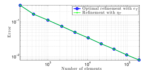
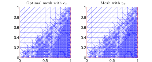
Refer to caption
Figure 2: Adaptive computation of Example 6, where the error is measured in the combined norm.
Refer to caption
Figure 3: Adaptive mesh after the fourth refinement in Example 6. There are 4823 elements in the optimal mesh, and 4878 elements in the mesh calculated with the help of ηTsubscript𝜂𝑇\eta_{T}.
Refer to caption
Figure 4: One of the most fine parts in the final adaptive mesh in Example 6.
Table 6: Adaptive computation of Example 6. The number of elements in the optimal meshes and the meshes generated by the help of ηTsubscript𝜂𝑇\eta_{T}.
Ref. optimal with ηTsubscript𝜂𝑇\eta_{T} difference difference %percent\%
- 200 200 0 0
1 434 434 0 0
2 998 1002 4 0.40
3 2240 2252 12 0.53
4 4823 4878 55 1.14
5 10378 10446 68 0.65
6 22116 22337 221 0.99
7 46388 46768 380 0.81
8 96859 97832 973 1.00
9 198704 200970 2266 1.14
Example 7.

We take the 2D-eddy-current problem of Section 4.3 in the L𝐿L-shaped domain Ω:=(0,1)2([1/2,1]×[0,1/2])assignΩsuperscript012121012\Omega:=(0,1)^{2}\setminus\big{(}[\nicefrac{{1}}{{2}},1]\times[0,\nicefrac{{1}}{{2}}]\big{)} with ϵ=iditalic-ϵid\epsilon=\operatorname{id}, μ=1000𝜇1000\mu=1000 and J=[1,0]𝐽superscript10topJ=[1,0]^{\top}. We set zero Dirichlet boundary conditions on the whole boundary, i.e., Γ𝙳=ΓsubscriptΓ𝙳Γ\Gamma_{\mathtt{D}}=\Gamma and Γ𝙽=subscriptΓ𝙽\Gamma_{\mathtt{N}}=\emptyset. The exact solution of this problem is unknown. However, since the majorant gives indeed the exact error in the combined norm, we will use this information in this example. Therefore, all the error values in Figure 5 and Table 7 are actually the values of the majorant. We compare uniform refinement and adaptive refinement using ηTsubscript𝜂𝑇\eta_{T} with

ηT2=ec(E𝚑,H𝚑)T=|JE𝚑H𝚑|𝖫2(T)2+|H𝚑μ1rotE𝚑|𝖫2(T),μ2,superscriptsubscript𝜂𝑇2subscriptecsubscriptsubscript𝐸𝚑subscript𝐻𝚑𝑇superscriptsubscript𝐽subscript𝐸𝚑superscriptbottomsubscript𝐻𝚑superscript𝖫2𝑇2superscriptsubscriptsubscript𝐻𝚑superscript𝜇1rotsubscript𝐸𝚑superscript𝖫2𝑇𝜇2\eta_{T}^{2}=\mathcal{M}_{\mathrm{ec}}(E_{\mathtt{h}},H_{\mathtt{h}})_{T}=|J-E_{\mathtt{h}}-\nabla^{\bot}H_{\mathtt{h}}|_{\operatorname{\sf L}^{2}(T)}^{2}+|H_{\mathtt{h}}-\mu^{-1}\operatorname{rot}E_{\mathtt{h}}|_{\operatorname{\sf L}^{2}(T),\mu}^{2},

refining 30%percent3030\% of elements on each refinement iteration as before. We solve the primal and dual problems with linear Nédélec elements and linear Courant elements, respectively. The resulting linear systems are solved directly. We see from Figure 5 that the adaptive procedure is beneficial in this example. We have also depicted the approximation in Figure 6 and the mesh in Figure 7 after the fifth refinement. It can be concluded that in addition to providing the exact error, the majorant also provides a good error indicator without any additional computational expenditures.
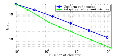
Refer to caption
Figure 5: Adaptive computation of Example 7.
Table 7: Example 7 (2D-eddy-current) Adaptively refined meshes.
N𝚎𝚕𝚎𝚖subscript𝑁𝚎𝚕𝚎𝚖N_{\mathtt{elem}} ec(E𝚑,H𝚑)1/2subscriptecsuperscriptsubscript𝐸𝚑subscript𝐻𝚑12\mathcal{M}_{\mathrm{ec}}(E_{\mathtt{h}},H_{\mathtt{h}})^{\!\nicefrac{{1}}{{2}}} ec(E𝚑,H𝚑)1/2/|J|𝖫2subscriptecsuperscriptsubscript𝐸𝚑subscript𝐻𝚑12subscript𝐽superscript𝖫2\mathcal{M}_{\mathrm{ec}}(E_{\mathtt{h}},H_{\mathtt{h}})^{\!\nicefrac{{1}}{{2}}}/|J|_{\operatorname{\sf L}^{2}}
96 0.2534 0.2926
230 0.1534 0.1771
541 0.0842 0.0973
1204 0.0467 0.0539
2623 0.0309 0.0357
6082 0.0203 0.0234
13514 0.0135 0.0155
29530 0.0093 0.0107
63363 0.0062 0.0072
134205 0.0043 0.0050
Refer to captionE𝚑,1subscript𝐸𝚑1E_{\mathtt{h},1}E𝚑,2subscript𝐸𝚑2E_{\mathtt{h},2}H𝚑subscript𝐻𝚑H_{\mathtt{h}}
Figure 6: The two components of the approximate primal variable E𝚑subscript𝐸𝚑E_{\mathtt{h}} and the dual variable H𝚑subscript𝐻𝚑H_{\mathtt{h}} of Example 7 after the third adaptive refinement.
Refer to caption
Figure 7: Adaptive mesh after the fifth adaptive refinement in Example 7.
Example 8.

We take the 2D-eddy-current problem of Section 4.3 in Ω:=(0,1)2assignΩsuperscript012\Omega:=(0,1)^{2}. In order to define discontinuous data, we define with ξ(x):=ln(2+x2)assign𝜉𝑥2subscript𝑥2\xi(x):=\ln(2+x_{2}) and

Ω1subscriptΩ1\displaystyle\Omega_{1} :=((0,1)×(0.4,0.6))((0.3,0.5)×(0,1)),assignabsent010.40.60.30.501\displaystyle:=\big{(}(0,1)\times(0.4,0.6)\big{)}\cup\big{(}(0.3,0.5)\times(0,1)\big{)}, ϵ|Ω1evaluated-atitalic-ϵsubscriptΩ1\displaystyle\epsilon|_{\Omega_{1}} :=id,assignabsentid\displaystyle:=\operatorname{id}, ϵ|ΩΩ¯1evaluated-atitalic-ϵΩsubscript¯Ω1\displaystyle\epsilon|_{\Omega\setminus\overline{\Omega}_{1}} :=100id,assignabsent100id\displaystyle:=100\cdot\operatorname{id},
μ|Ω1evaluated-at𝜇subscriptΩ1\displaystyle\mu|_{\Omega_{1}} :=1000,assignabsent1000\displaystyle:=1000, μ|ΩΩ¯1evaluated-at𝜇Ωsubscript¯Ω1\displaystyle\mu|_{\Omega\setminus\overline{\Omega}_{1}} :=1,assignabsent1\displaystyle:=1,
Ω2subscriptΩ2\displaystyle\Omega_{2} :=(0,1)×(0.35,0.65),assignabsent010.350.65\displaystyle:=(0,1)\times(0.35,0.65), J|Ω2evaluated-at𝐽subscriptΩ2\displaystyle J|_{\Omega_{2}} :=ξ[10],assignabsent𝜉matrix10\displaystyle:=\xi\begin{bmatrix}1\\ 0\end{bmatrix}, J|ΩΩ¯2evaluated-at𝐽Ωsubscript¯Ω2\displaystyle J|_{\Omega\setminus\overline{\Omega}_{2}} :=ξ[01].assignabsent𝜉matrix01\displaystyle:=-\xi\begin{bmatrix}0\\ 1\end{bmatrix}.

We set zero Dirichlet boundary conditions on the right side of the rectanglular boundary and zero Neumann boundary condition on the remaining part, i.e., Γ𝙳={xΩx1=1}subscriptΓ𝙳conditional-set𝑥Ωsubscript𝑥11\Gamma_{\mathtt{D}}=\{x\in\Omega\,\mid\,x_{1}=1\}. As in Example 7, the exact solution of this problem is unknown, so the error values in Figure 8 and Table 8 are the values of the majorant. We compare uniform refinement and adaptive refinement using ηTsubscript𝜂𝑇\eta_{T} with

ηT2=ec(E𝚑,H𝚑)T=|JϵE𝚑H𝚑|𝖫2(T),ϵ12+|H𝚑μ1rotE𝚑|𝖫2(T),μ2,superscriptsubscript𝜂𝑇2subscriptecsubscriptsubscript𝐸𝚑subscript𝐻𝚑𝑇superscriptsubscript𝐽italic-ϵsubscript𝐸𝚑superscriptbottomsubscript𝐻𝚑superscript𝖫2𝑇superscriptitalic-ϵ12superscriptsubscriptsubscript𝐻𝚑superscript𝜇1rotsubscript𝐸𝚑superscript𝖫2𝑇𝜇2\eta_{T}^{2}=\mathcal{M}_{\mathrm{ec}}(E_{\mathtt{h}},H_{\mathtt{h}})_{T}=|J-\epsilon E_{\mathtt{h}}-\nabla^{\bot}H_{\mathtt{h}}|_{\operatorname{\sf L}^{2}(T),\epsilon^{-1}}^{2}+|H_{\mathtt{h}}-\mu^{-1}\operatorname{rot}E_{\mathtt{h}}|_{\operatorname{\sf L}^{2}(T),\mu}^{2},

refining 30%percent3030\% of elements on each refinement iteration as before. We solve the primal and dual problems with linear Nédélec elements and linear Courant elements, respectively. The resulting linear systems are solved directly. Again, we see from Figure 8 that the adaptive procedure is beneficial in this example. We have also depicted the approximation in Figure 9 and the mesh in Figure 10 after the third refinement.
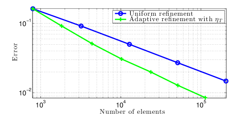
Refer to caption
Figure 8: Adaptive computation of Example 8.
Table 8: Example 8 (2D-eddy-current) Adaptively refined meshes.
N𝚎𝚕𝚎𝚖subscript𝑁𝚎𝚕𝚎𝚖N_{\mathtt{elem}} ec(E𝚑,H𝚑)1/2subscriptecsuperscriptsubscript𝐸𝚑subscript𝐻𝚑12\mathcal{M}_{\mathrm{ec}}(E_{\mathtt{h}},H_{\mathtt{h}})^{\!\nicefrac{{1}}{{2}}} ec(E𝚑,H𝚑)1/2/|J|𝖫2,ϵ1subscriptecsuperscriptsubscript𝐸𝚑subscript𝐻𝚑12subscript𝐽superscript𝖫2superscriptitalic-ϵ1\mathcal{M}_{\mathrm{ec}}(E_{\mathtt{h}},H_{\mathtt{h}})^{\!\nicefrac{{1}}{{2}}}/|J|_{\operatorname{\sf L}^{2},\epsilon^{-1}}
800 0.1632 0.2941
1827 0.0921 0.1659
4367 0.0513 0.0924
10214 0.0307 0.0554
23657 0.0199 0.0359
51429 0.0128 0.0231
113073 0.0085 0.0153
Refer to captionE𝚑,1subscript𝐸𝚑1E_{\mathtt{h},1}E𝚑,2subscript𝐸𝚑2E_{\mathtt{h},2}H𝚑subscript𝐻𝚑H_{\mathtt{h}}
Figure 9: The two components of the approximate primal variable E𝚑subscript𝐸𝚑E_{\mathtt{h}} and the dual variable H𝚑subscript𝐻𝚑H_{\mathtt{h}} of Example 8 after the third adaptive refinement.
Refer to caption
Figure 10: Adaptive mesh after the third adaptive refinement in Example 8.

To conclude, in all the tests performed, nonzero values of δ𝛿\delta were of magnitude 1018superscript101810^{-18}-1015superscript101510^{-15}. This is within the limit of machine precision, so numerically these numbers are considered zero. In addition to verifying the equality, we also performed three simple examples to show that the majorant can be used to perform refinement of element meshes without any additional computational expenditures.

Acknowledgements  We are deeply indebted to Sergey Repin for so many interesting and encouraging discussions. We thank him gratefully not only for being an academic colleague and teacher but also a good friend.

The first author also thanks Jan Valdman for showing how to program vectorized FEM solvers. The first author is funded by the Finnish foundations KAUTE Foundation and Väisälä Foundation of the Finnish Academy of Science and Letters.

This contribution has been worked out mainly while the first author was visiting the Fakultät für Mathematik of the Universität Duisburg-Essen during 2013.

References

  • [1] I. Anjam, O. Mali, A. Muzalevskiy, P. Neittaanmäki, and S. Repin. A posteriori error estimates for a Maxwell type problem. Russian J. Numer. Anal. Math. Modelling, 24(5):395–408, 2009.
  • [2] F. Brezzi and M. Fortin. Mixed and hybrid finite element methods. Springer, New York, 1991.
  • [3] V. Gol’dshtein, I. Mitrea, and M. Mitrea. Hodge decompositions with mixed boundary conditions and applications to partial differential equations on Lipschitz manifolds. J. Math. Sci. (N.Y.), 172(3):347–400, 2011.
  • [4] T. Jakab, I. Mitrea, and M. Mitrea. On the regularity of differential forms satisfying mixed boundary conditions in a class of Lipschitz domains. Indiana Univ. Math. J., 58(5):2043–2071, 2009.
  • [5] F. Jochmann. A compactness result for vector fields with divergence and curl in Lq(Ω)superscript𝐿𝑞Ω{L}^{q}({\Omega}) involving mixed boundary conditions. Appl. Anal., 66:189–203, 1997.
  • [6] P. Kuhn. Die Maxwellgleichung mit wechselnden Randbedingungen. Dissertation, Universität Essen, Fachbereich Mathematik, http://arxiv.org/abs/1108.2028, Shaker, 1999.
  • [7] O. Mali, A. Muzalevskiy, and D. Pauly. Conforming and non-conforming functional a posteriori error estimates for elliptic boundary value problems in exterior domains: Theory and numerical tests. Russian J. Numer. Anal. Math. Modelling, 28(6):577–596, 2013.
  • [8] O. Mali, P. Neittaanmäki, and S. Repin. Accuracy verification methods, theory and algorithms. Springer, 2014.
  • [9] P. Neittaanmäki and S. Repin. Reliable methods for computer simulation, error control and a posteriori estimates. Elsevier, New York, 2004.
  • [10] D. Pauly and S. Repin. Functional a posteriori error estimates for elliptic problems in exterior domains. J. Math. Sci. (N.Y.), 162(3):393–406, 2009.
  • [11] D. Pauly and S. Repin. Two-sided a posteriori error bounds for electro-magneto static problems. J. Math. Sci. (N.Y.), 166(1):53–62, 2010.
  • [12] D. Pauly, S. Repin, and Rossi T. Estimates for deviations from exact solutions of Maxwell’s initial boundary value problem. Ann. Acad. Sci. Fenn. Math., 36(2):661–676, 2011.
  • [13] T. Rahman and J. Valdman. Fast MATLAB assembly of FEM matrices in 2D and 3D: nodal elements. Appl. Math. Comput., 219(13):7151–7158, 2013.
  • [14] S. Repin. A posteriori estimates for partial differential equations. Walter de Gruyter (Radon Series Comp. Appl. Math.), Berlin, 2008.
  • [15] S. Repin. Estimates of deviations from exact solutions of initial boundary value problems for the wave equation. J. Math. Sci. (N. Y.), 159(2):229–240, 2009.
  • [16] S. Repin, S. Sauter, and A. Smolianski. Two-sided a posteriori error estimates for mixed formulations of elliptic problems. SIAM J. Numer. Anal., 45(3):928–945, 2007.