The reaction $\pi N\to\pi\pi N$ in chiral effective field theory
with explicit $\Delta(1232)$ degrees of freedom

Abstract

The reaction $\pi N\to\pi\pi N$ is studied at tree level up to next-to-leading order in the framework of manifestly covariant baryon chiral perturbation theory with explicit $\Delta(1232)$ degrees of freedom. Using total cross section data to determine the relevant low-energy constants, predictions are made for various differential as well as total cross sections at higher energies. A detailed comparison of results based on the heavy-baryon and relativistic formulations of chiral perturbation theory with and without explicit $\Delta$ degrees of freedom is given.

I Introduction

Chiral perturbation theory ($\chi$PT) is nowadays a standard tool to analyze low-energy hadronic reactions in harmony with the symmetries of QCD. It was originally formulated by Weinberg Weinberg:1978kz and, a few years later, extended and applied by Gasser and Leutwyler to study the low-energy dynamics of the Goldstone bosons at the one-loop level both in the SU(2) Gasser:1983yg and SU(3) Gasser:1984gg sectors. Starting with the pioneering work by Gasser et al. Gasser:1987rb , $\chi$PT has also been extensively used in the baryon sector, see Refs. Bernard:1995dp ; Bernard:2006gx ; Bernard:2007zu for review articles and references therein. In the framework of $\chi$PT, low-energy hadronic observables are calculated within the chiral expansion, where the expansion parameter $Q$ is defined as the ratio of the soft scales corresponding to external momenta, denoted generically by $q$, or the pion mass $M_{\pi}$, and the chiral symmetry breaking scale $\Lambda_{\chi}\sim 1$ GeV. While in the Goldstone boson sector the hard scale $\Lambda_{\chi}$ only enters the amplitude through values of the low-energy constants (LECs) so that pion loop integrals calculated using dimensional regularization (DR) automatically fulfill the chiral power counting, a special treatment of the nucleon mass $m_{N}\sim\Lambda_{\chi}$ is required in the baryon sector. The standard way to maintain the power counting in the nucleon sector is the use of the heavy-baryon (HB) version of the effective Lagrangian Jenkins:1990jv ; Bernard:1992qa . In the heavy-baryon formulation of chiral perturbation theory (HB$\chi$PT), the nucleon mass does not appear in the propagators and enters only in form of $1/m_{N}$-corrections to the vertices which leads to the same suppression of DR loop integrals as in the Goldstone boson sector. It is, however, known that the HB expansion has, for certain observables such as some of the nucleon electroweak and scalar form factors Bernard:1996cc ; Becher:1999he , a very limited range of convergence. It is then advantageous to use a manifestly Lorentz-invariant effective Lagrangian rather than its HB version. Power counting can still be maintained using the method of Becher and Leutwyler Becher:1999he to extract the soft (i.e. infrared singular) parts of the loop integrals leading to the so-called infrared regularized $\chi$PT. Alternatively, the proper chiral scaling of the loop integrals can be restored in the covariant framework by imposing the appropriate renormalization conditions as proposed in Refs. Gegelia:1999gf ; Fuchs:2003qc within the so-called extended on-mass-shell scheme (EOMS). We refer the reader to Ref. Bernard:2007zu for a detailed discussion and comparison of the various $\chi$PT formulations and their applications in the single-baryon sector, see also Ref. Epelbaum:2012ua for a recent application of these ideas in the two-nucleon sector.

Another popular idea to extend the range of applicability of $\chi$PT in the nucleon sector is based on the explicit treatment of the $\Delta$(1232), the close-by resonance with the excitation energy of $\Delta\equiv m_{\Delta}-m_{N}=293\mbox{ MeV}$. All effects of the $\Delta$ in the standard approach are encoded in LECs of pion-nucleon interactions beyond leading order. The small excitation energy of the $\Delta$ and its strong coupling to the $\pi N$ system lead, however, to unnaturally large values of certain LECs which can, potentially, spoil the convergence of the chiral expansion. One can, therefore, argue that the explicit inclusion of the $\Delta$ in $\chi$PT by treating the delta-nucleon mass splitting as a soft scale will allow to resum a certain class of important contributions and improve the convergence as compared to the $\Delta$-less theory Jenkins:1991es ; Hemmert:1997ye . The improved convergence of HB$\chi$PT-$\Delta$ compared to the standard HB$\chi$PT has indeed been confirmed for $\pi N$ scattering Fettes:2000bb , proton Compton scattering, see Lensky:2012ag and references therein, nuclear forces, see e.g. Kaiser:1998wa ; Krebs:2007rh ; Epelbaum:2007sq , and other processes, see Ref. Bernard:2007zu for a review. It should, however, be emphasized that the explicit inclusion of the $\Delta$ makes calculations in the covariant framework considerably more involved and also leads to the appearance of additional LECs.

In the present work we analyze in detail single pion production off nucleons from threshold up to the delta resonance region using various formulations of $\chi$PT. The reaction $\pi N\to\pi\pi N$ has already attracted considerable interest on the experimental and theoretical sides which, historically, goes back to the possibility of using this process for the extraction of the $\pi\pi$ scattering lengths (see Refs. Beringer:1992ic ; Bernard:1994wf ; Bernard:1995gx in the context of $\chi$PT and a more general discussion in Ref. Olsson:1995iy with references to earlier work). Single pion production off nucleons is also of special interest from the point of view of chiral perturbation theory. First of all, it involves three pions in the initial and final states so that one may expect for the scattering amplitude to be strongly constrained by the chiral symmetry of QCD. It therefore provides an excellent testing ground for $\chi$PT. On the other hand, the relatively high energies involved in this pion production reaction and the proximity of resonances with a strong coupling to the $\pi\pi N$ final state make the pursuit of a theoretical description of this reaction rather challenging. One expects for this process to be particularly well suited for studying the role of the $\Delta$ isobar, relativistic effects and unitarity and thus for testing various available formulations of $\chi$PT. Indeed, in Ref. Jensen:1997em a relativistic tree level calculation including the $\Delta$ and the Roper resonance with leading order pion-baryon vertices (i.e. dimension one couplings only) was performed and the appearing parameters were determined from other sources. The resulting total and differential cross section data were generally well described, encouraging further studies in baryon chiral perturbation theory. Last but not least, it is worth mentioning that the reaction $\pi N\to\pi\pi N$ provides complementary information to pion-nucleon scattering in the sense that it is sensitive to certain LECs which cannot be extracted from the $\pi N$ system. The most prominent example is the LEC $d_{16}$ which governs the quark mass dependence of the nucleon axial vector coupling constant. As a matter of fact, the lack of knowledge of its precise value represents one of the main sources of theoretical uncertainty in chiral extrapolations of nuclear observables Epelbaum:2002gb ; Epelbaum:2002gk ; Beane:2002vs ; Beane:2002xf ; Berengut:2013nh ; Epelbaum:2012iu ; Epelbaum:2013wla .

All these arguments provide a strong motivation to take a fresh look at the reaction $\pi N\to\pi\pi N$ in the framework of $\chi$PT. In Refs. Bernard:1995gx and Fettes:1999wp , it was analyzed within HB$\chi$PT at tree- and leading one-loop levels, respectively. A tree-level calculation based on the relativistic pion-nucleon Lagrangian is reported in Ref. Bernard:1997tq . The role of unitarity corrections in a heavy baryon calculation was in particular stressed in Ref. Mobed:2005av . While these studies already showed that the predictions of chiral perturbation theory are in a satisfactory agreement with experimental data, we expect to be able to improve on them in the delta region by explicitly taking into account the delta degrees of freedom systematically, extending the earlier work of Ref. Jensen:1997em . To the best of our knowledge, no calculations of this reaction using $\chi$PT with explicit $\Delta$’s beyond the leading order pion-baryon couplings has been performed. In this paper we fill this gap and study single pion production off nucleons in the framework of relativistic baryon $\chi$PT with explicit $\Delta$ degrees of freedom at complete tree level with the inclusion of the terms from the dimension-two effective Lagrangian.

Our paper is organized as follows. In section II we discuss the relevant terms in the effective pion-nucleon-delta Lagrangian. The decomposition of the transition matrix elements into the corresponding invariant amplitudes is considered in section III while the relevant observables are defined in section V. Section IV specifies all tree-level contributions to the amplitude up to next-to-leading order. The details of the calculation and the fitting procedure can be found in section VI, while predictions for observables not used in the fitting procedure are collected in section VII. Finally, the main results of our study are summarized in section VIII. The appendix contains explicit expressions for the kinematical variables and weight functions we are using.

II Effective Lagrangian

We employ the so-called small scale expansion (SSE) or $\varepsilon$-expansion throughout this work with the expansion parameter being defined as Hemmert:1997ye

$$\varepsilon\in\left\{\frac{q}{\Lambda_{\chi}},\frac{M_{\pi}}{\Lambda_{\chi}},\frac{\Delta}{\Lambda_{\chi}}\right\}\,,$$ (1)

i.e. the delta-nucleon mass splitting is treated on the same footing as the pion mass, see however Ref. Pascalutsa:2002pi for an alternative power counting scheme. We now discuss the terms in the effective Lagrangian relevant for our calculation.

The relativistic effective Lagrangian needed to describe pion-nucleon dynamics at tree level consists of the following pieces (see Ref. Fettes:2000gb for a full list of terms)

$$\mathcal{L}_{\mathrm{eff}}=\mathcal{L}_{\pi\pi}^{(2)}+\mathcal{L}_{\pi N}^{(1)}+\mathcal{L}_{\pi N}^{(2)}+\mathcal{L}_{\pi\Delta}^{(1)}+\mathcal{L}_{\pi\Delta}^{(2)}+\mathcal{L}_{\pi N\Delta}^{(1)}+\mathcal{L}_{\pi N\Delta}^{(2)}\;\text{,}$$ (2)

where the superscripts refer to the chiral dimension. The first term in Eq. (2) describes the meson interaction

$$\mathcal{L}_{\pi\pi}^{(2)} =\frac{F_{\pi}^{2}}{4}\braket{\partial_{\mu}U^{\dagger}\partial^{\mu}U}+\frac{F_{\pi}^{2}B}{2}\braket{\mathcal{M}U^{\dagger}+U\mathcal{M}}\;\text{,}$$ (3)

where the pions are collected in the SU(2) matrix-valued field $U(x)=u(x)^{2}$ given by

$$U=1+\mathrm{i}\frac{\bm{\tau}\cdot\bm{\pi}}{F_{\pi}}-\frac{\bm{\pi}^{2}}{2F_{\pi}^{2}}-\mathrm{i}\alpha\frac{\bm{\pi}^{2}\bm{\tau}\cdot\bm{\pi}}{F_{\pi}^{3}}+\frac{(8\alpha-1)}{8F_{\pi}^{4}}\bm{\pi}^{4}+\ldots\,,$$ (4)

where $\alpha$ is a constant representing the freedom in the definition of the pion field. Further, $F_{\pi}$ is the pion decay constant, $\mathcal{M}={\rm diag}(m_{u},\,m_{d})$ is the quark mass matrix and $B$ is a low-energy constant.

The next two terms in Eq. (2) give the leading and subleading pion-nucleon Lagrangians

$$\begin{aligned} \mathcal{L}_{\pi N}^{(1)}&=\mathrm{bar}{\Psi}\left[\mathrm{i}\not{D}-m_{N}+\frac{g_{A}}{2}\not{u}\gamma_{5}\right]\Psi\;\text{,}\\ \mathcal{L}_{\pi N}^{(2)}&=\mathrm{bar}{\Psi}\left[c_{1}\Braket{\chi_{+}}+c_{2}\left(-\frac{1}{8m_{N}^{2}}\braket{u_{\mu}u_{\nu}}\{D^{\mu},D^{\nu}\}+\mathrm{h.c.}\right)+\frac{c_{3}}{2}\Braket{u\cdot u}\right.\\ &\qquad\left.-\frac{c_{4}}{8}[\gamma^{\mu},\gamma^{\nu}][u_{\mu},u_{\nu}]+c_{5}\Big{(}\chi_{+}-\frac{\braket{\chi_{+}}}{2}\Big{)}\right]\Psi\;\text{,}\end{aligned}$$ (5)

where $m_{N}$ and $g_{A}$ denote the nucleon mass and axial vector coupling, $c_{i}$’s refer to further LECs and the proton and neutron are given in the isodoublet representation

$$\Psi=\begin{pmatrix}p\\ n\end{pmatrix}\;\text{.}$$ (6)

The covariant derivative in Eq. (5) in the absence of external sources is defined via:

$$D_{\mu}=\partial_{\mu}+\Gamma_{\mu}\ \qquad\mathrm{with}\qquad\Gamma_{\mu}=\frac{1}{2}(u^{\dagger}\partial_{\mu}u+u\,\partial_{\mu}u^{\dagger})\;\text{.}$$ (7)

In addition, the abbreviation

$$\chi_{+}=u^{\dagger}\chi u^{\dagger}+u\chi^{\dagger}u\qquad\mathrm{with}\qquad\chi=2B_{0}\mathcal{M}$$ (8)

and the chiral vielbein

$$u_{\mu}=\mathrm{i}(u^{\dagger}\partial_{\mu}u-u\,\partial_{\mu}u^{\dagger})$$ (9)

are used.

The inclusion of the $\Delta(1232)$ as an explicit degree of freedom adds the four last terms to the effective Lagrangian in Eq. (2). The delta isobar is described by a Rarita-Schwinger isospurion $\Psi_{\mu}^{i}\;\text{,}$ a spin-$3/2$ field, which is constructed via coupling of a spin-$1$ to a spin-$1/2$ field, treated as an isodoublet with an additional isovector index $i\in\{1,2,3\}$. The pion-delta Lagrangian up to second order reads Hemmert:1997ye ; Fettes:2000bb

$$\begin{aligned} \mathcal{L}_{\pi\Delta}^{(1)}&=-\mathrm{bar}{\Psi}_{i}^{\mu}\Big{[}(\mathrm{i}\not{D}^{ij}-m_{\Delta}\delta^{ij})g_{\mu\nu}-\mathrm{i}(\gamma_{\mu}D_{\nu}^{ij}+\gamma_{\nu}D_{\nu}^{ij})+\mathrm{i}\gamma_{\mu}\not{D}^{ij}\gamma_{\nu}+m_{\Delta}\delta^{ij}\gamma_{\mu}\gamma_{\nu}\\ &\qquad+\frac{g_{1}}{2}g_{\mu\nu}\not{u}^{ij}\gamma_{5}+\frac{g_{2}}{2}(\gamma_{\mu}u_{\nu}^{ij}+u_{\mu}^{ij}\gamma_{\nu})\gamma_{5}+\frac{g_{3}}{2}\gamma_{\mu}\not{u}^{ij}\gamma_{5}\gamma_{\nu}\Big{]}\Psi^{\nu}_{j}\;\text{,}\\ \mathcal{L}_{\pi\Delta}^{(2)}&=\frac{c_{1}^{\Delta}}{2}\mathrm{bar}{\Psi}_{\mu}^{i}\Theta^{\mu\alpha}(z)\gamma_{\alpha\beta}\delta^{ij}\braket{\chi_{+}}\Theta^{\beta\nu}(z)\Psi_{\nu}^{j}+\mathrm{h.c.}+\ldots\,,\end{aligned}$$ (10)

where terms with two and more pion fields in $\mathcal{L}_{\pi\Delta}^{(2)}$ are not shown since they do not contribute to the reaction $\pi N\to\pi\pi N$ at order $\varepsilon^{2}$. Here, the quantity $\Theta^{\mu\alpha}(z)$ is defined via $\Theta^{\mu\alpha}(z)=g^{\mu\alpha}+z\gamma^{\mu}\gamma^{\alpha}$ and $z$, $g_{2}$ and $g_{3}$ denote the so-called off-shell parameters. Notice that the dependence of the amplitude on such off-shell parameters can be absorbed into a redefinition of the corresponding LECs, see Refs. Tang:1996sq ; Pascalutsa:2000kd ; Krebs:2009bf for more details. It is, therefore, convenient to choose

$$z=g_{2}=g_{3}=0,$$ (11)

which specifies our conventions for the calculations in the manifestly covariant framework. Here and in what follows, we show explicitly the dependence on some of the off-shell parameters in order to maintain consistency between the covariant and HB calculations as will be explained below. The covariant derivative in Eq. (10) is given by

$$D^{ij}_{\mu}=\partial_{\mu}\delta^{ij}+\Gamma_{\mu}^{ij}\qquad\mathrm{with}\qquad\Gamma_{\mu}^{ij}=\Gamma_{\mu}\delta^{ij}-\mathrm{i}\epsilon^{ijk}\braket{\tau^{k}\Gamma_{\mu}}\;\text{.}$$ (12)

Finally, the pion-nucleon-delta Lagrangian reads Hemmert:1997ye ; Fettes:2000bb

$$\mathcal{L}_{\pi N\Delta}^{(1)} =h_{A}\left[\mathrm{bar}{\Psi}_{\mu}^{i}\Theta^{\mu\alpha}(z)w_{\alpha}^{i}\Psi_{N}+\mathrm{bar}{\Psi}w^{i}_{\alpha}\Theta^{\alpha\mu}(z)\Psi_{\mu}^{i}\right]\;\text{,}$$ (13)

$$\mathcal{L}_{\pi N\Delta}^{(2)} =\mathrm{bar}{\Psi}_{\mu}^{i}\Theta^{\mu\alpha}(z)\left[\mathrm{i}b_{3}w_{\alpha\beta}^{i}\gamma^{\beta}+\frac{b_{4}}{2}w_{\alpha}^{i}w_{\beta}^{j}\gamma^{\beta}\gamma_{5}\tau^{j}+\frac{b_{5}}{2}w_{\alpha}^{j}w_{\beta}^{i}\gamma^{\beta}\gamma_{5}\tau^{j}+\frac{b_{6}}{m_{N}}\mathrm{i}w_{\alpha\beta}^{i}\mathrm{i}D^{\beta}\right]\Psi+\mathrm{h.c.},$$

where $h_{A}$ is the $\pi N\Delta$ axial coupling, $b_{i}$ are further LECs and

$$w_{\alpha}^{i} =\frac{1}{2}\mathrm{Tr}\left[\tau^{i}u_{\alpha}\right]\qquad\mathrm{and}\qquad w_{\alpha\beta}^{i} =\frac{1}{2}\mathrm{Tr}\left[\tau^{i}\left[D_{\alpha},u_{\beta}\right]\right]\;\text{.}$$ (14)

It should be emphasized that the free spin-3/2 Lagrangian is non-unique and usually written in terms of an unphysical “gauge” parameter $A$, whose entire dependence of the observables can be absorbed into redefinition of the delta field. We have not shown explicitly the dependence on the parameter $A$ in the effective Lagrangian by making the choice $A=-1$. This particular choice is convenient in the covariant approach since it leads to the simplest form of the free Lagrangian and thus also of the free delta propagator

$$\mathcal{G}^{\mu\nu}_{\Delta}(p)=-\frac{\not{p}+m_{\Delta}}{p^{2}-m_{\Delta}^{2}}\left(g^{\mu\nu}-\frac{1}{3}\gamma^{\mu}\gamma^{\nu}+\frac{1}{3}\frac{p^{\mu}\gamma^{\nu}-p^{\nu}\gamma^{\mu}}{m_{\Delta}}-\frac{2}{3}\frac{p^{\mu}p^{\nu}}{m_{\Delta}^{2}}\right)\;\text{.}$$ (15)

Since we are particularly interested here in the role of relativistic effects, we will also carry out the calculations within HB$\chi$PT. In this approach, the nucleon four-momentum $p_{\mu}$ is separated into a large piece close to the on-shell kinematics and a soft residual contribution $k_{\mu}$ via

$$p_{\mu}=m_{N}\,v_{\mu}+k_{\mu}$$ (16)

with $v_{\mu}$ being the four-velocity of the nucleon with the properties $v^{2}=1$ and $v^{0}\geq 1$. The nucleon field $\Psi$ is decomposed into eigenstates of $\not{v}$ with eigenvalues $+1$ and $-1$, the so-called ”light” and ”heavy” fields, respectively,

$$N_{v} =e^{\mathrm{i}m_{N}v\cdot x}P_{v}^{+}\Psi\;\text{,}$$ (17)

$$h_{v} =e^{\mathrm{i}m_{N}v\cdot x}P_{v}^{-}\Psi$$

with the projection operators $P_{v}^{\pm}=\frac{1}{2}(1\pm\not{v})$. $N_{v}$ and $h_{v}$ correspond to the upper- and lower-components of a Dirac spinor and thus positive and negative energy solutions, respectively. The effects of the $h_{v}$-components at low energies can be interpreted as contact terms so that the resulting Lagrangian involves only $N_{v}$ and its derivatives. Analogously, the delta resonance is included by defining a ”light” spin-$3/2$ and isospin-$3/2$ field

$$T^{\mu}_{i} =e^{\mathrm{i}m_{N}v\cdot x}P^{+}_{v}\xi^{3/2}_{ij}\left(P^{3/2}_{33}\right)^{\mu\nu}\Psi_{\nu}^{j}$$ (18)

with the spin and isospin projection operators $P^{3/2}_{33}$ and $\xi^{3/2}_{ij}$, respectively. The other “heavy” component is integrated out of the action. For more details on the heavy-baryon expansion in the pion-nucleon-delta sector the reader is referred to Refs. Hemmert:1997ye ; Fettes:2000bb . For the calculation at order $\epsilon^{2}$, the required heavy-baryon effective Lagrangian involves the following pieces

$$\mathcal{\hat{L}}_{\mathrm{eff}} =\mathcal{L}_{\pi\pi}^{(2)}+\mathcal{\hat{L}}_{\pi N}^{(1)}+\mathcal{\hat{L}}_{\pi N}^{(2)}+\mathcal{\hat{L}}_{\pi\Delta}^{(1)}+\mathcal{\hat{L}}_{\pi\Delta}^{(2)}+\mathcal{\hat{L}}_{\pi N\Delta}^{(1)}+\mathcal{\hat{L}}_{\pi N\Delta}^{(2)}.$$ (19)

The explicit form of the nucleon terms can be found in Fettes:2000gb while the delta terms are given in Ref. Hemmert:1997ye . We emphasize, however, that the authors of Ref. Hemmert:1997ye , whose results for the HB effective Lagrangian are adopted in our work, made a choice for the gauge parameter $A=0$ without specifying the values of the off-shell parameters. In order to be consistent with the convention used in the covariant calculations, see Eq. (11), one has to choose in the HB framework

$$\hat{z}=-\frac{1}{2}\;\text{,}\qquad\hat{g}_{2}=-g_{1}\;\text{,}\qquad\hat{g}_{3}=-g_{1}\,,$$ (20)

see Ref. Krebs:2013 for more details.

III Invariant Amplitudes

In this section we discuss the decomposition of the $T$-matrix for the reaction $\pi N\to\pi\pi N$ in terms of the corresponding invariant amplitudes, following Ref. Bernard:1997tq . Throughout this work, the kinematical variables are defined as follows:

$$\pi^{a}(q_{1})\,N(p=m_{N}v+k)\;\to\;\pi^{b}(q_{2})\,\pi^{c}(q_{3})\,N^{\prime}(p^{\prime}=m_{N}v+k^{\prime})\;\text{,}$$ (21)

where $N$ denotes a nucleon and $\pi^{a}$ a pion with the isospin quantum number $a$.

III.1 Relativistic chiral perturbation theory

In the relativistic case, the $T$-matrix can be expressed in terms of four invariant amplitudes $F_{i}$ ($i\in\{1,2,3,4\}$) which depend on the five Mandelstam variables

$$s=(p+q_{1})^{2}\;\text{,}\quad s_{1}=(q_{2}+p^{\prime})^{2}\;\text{,}\quad s_{2}=(q_{3}+p^{\prime})^{2}\;\text{,}\quad t_{1}=(q_{2}-q_{1})^{2}\;\text{,}\quad t_{2}=(q_{3}-q_{1})^{2}\;\text{.}$$ (22)

The spin structure of the $T$-matrix can be parametrized in the following way

$$T_{ss^{\prime}}^{abc}=\mathrm{i}\mathrm{bar}{u}^{(s^{\prime})}\gamma_{5}\left(F_{1}^{abc}+(\not{q}_{2}+\not{q}_{3})F_{2}^{abc}+(\not{q}_{2}-\not{q}_{3})F_{3}^{abc}+(\not{q}_{2}\not{q}_{3}-\not{q}_{3}\not{q}_{2})F_{4}^{abc}\right)u^{(s)},$$ (23)

where the superscripts on the spinors $\mathrm{bar}u,u$ refer to the spin. The isospin decomposition of the invariant amplitudes reads

$$F_{i}^{abc}=\chi_{N^{\prime}}^{\dagger}\left(\tau^{a}\delta^{bc}B_{i}^{1}+\tau^{b}\delta^{ac}B_{i}^{2}+\tau^{c}\delta^{ab}B_{i}^{3}+\mathrm{i}\epsilon^{abc}B_{i}^{4}\right)\chi_{N}.$$ (24)

Here, the $B_{i}$’s have the following symmetry under exchange of the two outgoing particles

$$B_{i}^{2}(s,s_{1},s_{2},t_{1},t_{2})=\epsilon_{i}B_{i}^{3}(s,s_{2},s_{1},t_{2},t_{1})\;\text{,}\qquad\epsilon_{1,2}=1\;\text{,}\qquad\epsilon_{3,4}=-1\;\text{.}$$ (25)

In the five physically accessible channels, the amplitudes contributing to each channel reduce to

$$\begin{aligned} &\mathrm{I.}&\pi^{-}p&\to\pi^{0}\pi^{0}n:&F_{i}&=\sqrt{2}B_{i}^{1}\\ &\mathrm{II.}&\pi^{-}p&\to\pi^{+}\pi^{-}n:&F_{i}&=\sqrt{2}(B_{i}^{1}+B_{i}^{2})\\ &\mathrm{III.}&\pi^{+}p&\to\pi^{+}\pi^{+}n:&F_{i}&=\sqrt{2}(B_{i}^{2}+B_{i}^{3})\\ &\mathrm{IV.}&\pi^{+}p&\to\pi^{+}\pi^{0}p:&F_{i}&=B_{i}^{3}+B_{i}^{4}\\ &\mathrm{V.}&\pi^{-}p&\to\pi^{0}\pi^{-}p:&F_{i}&=B_{i}^{2}+B_{i}^{4}\;\text{.}\end{aligned}$$ (26)

The unpolarized invariant matrix element squared in the relativistic formalism has the form

$$|\mathcal{M}|^{2}=\frac{1}{2}\sum_{s,s^{\prime}}T^{\dagger}_{ss^{\prime}}T_{ss^{\prime}}=\sum_{i,j=1}^{4}\frac{y_{ij}}{4m_{N}^{2}}F_{i}^{*}F_{j},$$ (27)

with the weight functions $y_{ij}=y_{ji}$ given by the trace over the respective Dirac structures (see Appendix A).

III.2 Heavy-baryon chiral perturbation theory

In the heavy-baryon framework, the spin structure of an amplitude is given by a combination of the non-commuting Pauli-Lubanski spin vectors $S_{\mu}$. In the case of $\pi N\to\pi\pi N$, the transition matrix can be written in terms of four invariant amplitudes $A$, $B$, $C$ and $D$ which depend on the five momenta $k$, $k^{\prime}$, $q_{1}$, $q_{2}$ and $q_{3}$ and are defined via Fettes:1999wp

$$T_{ss^{\prime}}^{abc}=\mathrm{bar}{u}_{v}^{(s^{\prime})}\left(S\cdot q_{1}\,A^{abc}+S\cdot q_{2}\,B^{abc}+S\cdot q_{3}\,C^{abc}+\mathrm{i}\epsilon_{\mu\nu\alpha\beta}\,q_{1}^{\mu}q_{2}^{\nu}q_{3}^{\alpha}v^{\beta}\,D^{abc}\right)u_{v}^{(s)}.$$ (28)

Here, the heavy-baryon spinor $u_{v}^{(s)}$ is given in the Pauli spinor representation

$$u_{v}^{(s)}(p)=P_{v}^{+}u^{(s)}(p)=\mathcal{N}\begin{pmatrix}\chi_{s}\\ 0\end{pmatrix}\;\text{.}$$ (29)

The normalization factor

$$\mathcal{N}=\sqrt{\frac{p^{0}+m_{N}}{2m_{N}}}$$ (30)

ensures the proper matching to the relativistic theory and has to be taken into account in the $1/m_{N}$ expansion,

$$\mathcal{N}\mathcal{N}^{\prime}=1+\mathcal{O}\left(\frac{1}{m_{N}^{2}}\right)\;\text{.}$$ (31)

Thus, for a tree level calculation, the normalization factors can be set equal to $1$. The isospin decomposition is the same as in the relativistic case, namely

$$X^{abc}=\chi_{N^{\prime}}^{\dagger}\left(\tau^{a}\delta^{bc}X_{1}+\tau^{b}\delta^{ac}X_{2}+\tau^{c}\delta^{ab}X_{3}+\mathrm{i}\epsilon^{abc}X_{4}\right)\chi_{N}\;\text{,}\quad X\in\{A,B,C,D\}$$ (32)

and thus the reduction in the five physically accessible channels is the same

$$\mathrm{I.} \pi^{-}p \to\pi^{0}\pi^{0}n: X =\sqrt{2}X_{1}$$ (33)

$$\mathrm{II.} \pi^{-}p \to\pi^{+}\pi^{-}n: X =\sqrt{2}(X_{1}+X_{2})$$

$$\mathrm{III.} \pi^{+}p \to\pi^{+}\pi^{+}n: X =\sqrt{2}(X_{2}+X_{3})$$

$$\mathrm{IV.} \pi^{+}p \to\pi^{+}\pi^{0}p: X =X_{3}+X_{4}$$

$$\mathrm{V.} \pi^{-}p \to\pi^{0}\pi^{-}p: X =X_{2}+X_{4}\;\text{.}$$

The unpolarized invariant matrix element squared in the heavy-baryon formalism reads

$$|\mathcal{M}|^{2} =\frac{1}{2}\sum_{s,s^{\prime}}T^{\dagger}_{ss^{\prime}}T_{ss^{\prime}}$$ (34)

$$=\frac{1}{4}\Big{[}|A|^{2}\bm{q}_{1}^{2}+|B|^{2}\bm{q}_{2}^{2}+|C|^{2}\bm{q}_{3}^{2}+(A^{*}B+AB^{*})\bm{q}_{1}\cdot\bm{q}_{2}+(A^{*}C+AC^{*})\bm{q}_{1}\cdot\bm{q}_{3}$$

$$+(B^{*}C+BC^{*})\bm{q}_{2}\cdot\bm{q}_{3}+4|D|^{2}\bm{q}_{1}^{2}\bm{q}_{2}^{2}\bm{q}_{3}^{2}(1-x_{1}^{2})(1-x_{2}^{2})\Big{(}1-\frac{(z-x_{1}x_{2})^{2}}{(1-x_{1}^{2})(1-x_{2}^{2})}\Big{)}\Big{]}\;\text{,}$$

where $x_{1}$, $x_{2}$ and $z$ are the cosines of the angles between $\bm{q}_{1}$ and $\bm{q}_{2}$, $\bm{q}_{1}$ and $\bm{q}_{3}$, and $\bm{q}_{2}$ and $\bm{q}_{3}$, respectively.

IV Tree-level contributions to the scattering amplitude

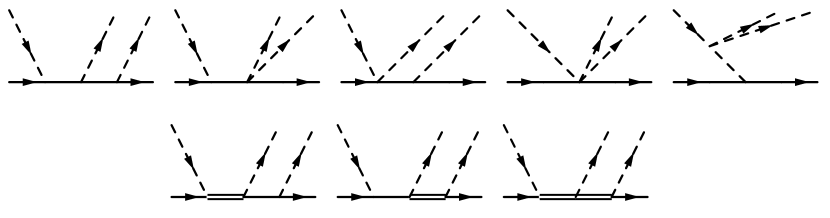
Figure 1: LO graphs for the reaction $\pi N\to\pi\pi N$. Nucleons and pions are denoted by solid and dashed lines, respectively. Delta is denoted by a double solid line. Crossed diagrams are not shown.

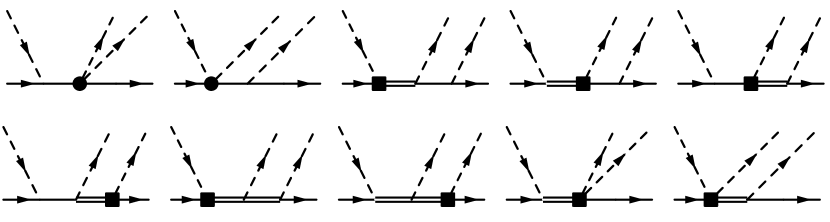
Figure 2: NLO graphs for the reaction $\pi N\to\pi\pi N$. The filled blob (filled square) denotes an insertion of the $c_{i}$- ($b_{i}$-) vertices. Crossed diagrams are not shown.

The leading-order (LO) and next-to-leading order (NLO) diagrams emerging at orders $\varepsilon^{1}$ and $\varepsilon^{2}$ in the SSE in the relativistic framework are shown in Fig. 1 and Fig. 2, respectively. The LO diagrams are constructed solely from the lowest-order vertices and thus depend only on the well-known LECs $F_{\pi}$, $g_{A}$ and the pion-nucleon-delta axial constant $h_{A}$. Subleading diagrams involve a single insertion of the LECs $c_{i}$ from $\mathcal{L}_{\pi N}^{(2)}$, which are known from pion-nucleon scattering or $b_{i}$ from $\mathcal{L}_{\pi N\Delta}^{(2)}$. We do not show diagrams involving an insertion of the LEC $c_{1}^{\Delta}$ whose contributions are taken into account by using the physical values of the mass of the delta isobar.

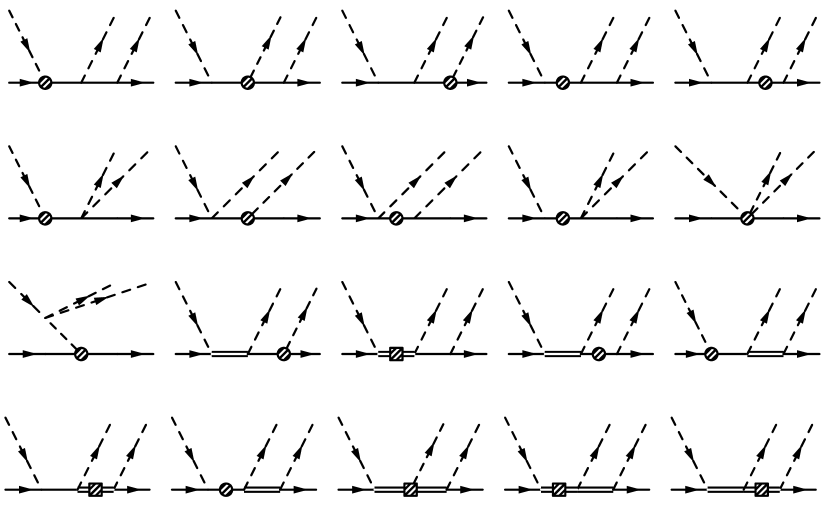
Figure 3: Additional NLO graphs contributing to the reaction $\pi N\to\pi\pi N$ in the heavy-baryon framework. The shaded blob/square denotes a pure $1/m_{N}$ insertion. Crossed diagrams are not shown.

When performing the calculation within the heavy-baryon framework, one needs to take into account additional diagrams involving $1/m_{N}$-vertices shown in Fig. 3. Notice that these vertices are fixed by the Poincaré invariance and do not involve any additional parameters.

We further emphasize that given the fact that the delta isobar is an unstable particle, it is not appropriate to use the free delta propagator given in Eqs. (15) in the resonance region corresponding to $p^{2}\sim m_{\Delta}^{2}$. In particular, a dressing of the delta becomes necessary, resumming all one-delta-irreducible diagrams which obviously become large in the kinematical region with $p^{2}-m_{\Delta}^{2}=\mathcal{O}(M_{\pi}^{2})$, see Ref. Pascalutsa:2002pi for details. Here we will take this effect into account using the following simple expressions for the $\Delta$ propagator where in particular the imaginary part of the derivative of the self-energy has been neglected, see Ref. Pascalutsa:2002pi . In the relativistic framework it reads

$$\mathcal{G}^{\mu\nu}_{\Delta}(p)=-\frac{\not{p}+m_{\Delta}}{p^{2}-m_{\Delta}^{2}+\mathrm{i}m_{\Delta}\Gamma}\left(g^{\mu\nu}-\frac{1}{3}\gamma^{\mu}\gamma^{\nu}+\frac{1}{3}\frac{p^{\mu}\gamma^{\nu}-p^{\nu}\gamma^{\mu}}{m_{\Delta}}-\frac{2}{3}\frac{p^{\mu}p^{\nu}}{m_{\Delta}^{2}}\right)\;\text{,}$$ (35)

with $\Gamma$ being the decay width of the $\Delta(1232)$ resonance, while the expression in the heavy-baryon framework has a simpler form

$$\mathcal{\hat{G}}_{\Delta}^{\mu\nu}(p)=\frac{-1}{v\cdot k-\Delta+\frac{\mathrm{i}}{2}\Gamma}\left(P^{3/2}_{33}\right)^{\mu\nu}\xi^{ij}_{3/2}\;\text{.}$$ (36)

At the level of accuracy of our calculations this should be completely sufficient. In fact, in Ref. Jensen:1997em the energy dependence of the width was incorporated. A more refined and consistent treatment of the delta propagator will be done in a future work.

While “dressing” of the delta is, strictly speaking, only required in the resonance region, we will use the expressions in Eqs. (35) and (36) for the Delta propagator in all diagrams and for all kinematical regions. Given that $\Gamma\sim\mathcal{O}(M_{\pi}^{3})$, such a procedure affects contributions to the amplitude at orders $\epsilon^{3}$ which are beyond the scope of the present work.

For the nucleonic contributions to the scattering amplitude, the results within the covariant and heavy-baryon frameworks we obtain agree with the ones published in Refs. Bernard:1995gx and Fettes:1999wp . The expressions for the delta contributions to the amplitude are too involved to be given here but can be made available as a Mathematica notebook upon request.

V Observables

To match the conventions adopted by the experimentalists, one needs to calculate the differential cross sections with respect to different kinematical variables. In particular, there are differential cross sections with respect to the outgoing pion energies and solid angles. Thus, it is advantageous to express the integration variables in spherical coordinates and pion energies. There is a second set of differential cross sections, which are with respect to the kinematics of the final dipion system. These can be derived from the first set.

The experimentalists’ convention suggests to choose the coordinate frame such that $\bm{q}_{1}$ defines the $z$-direction and $\bm{q}_{2}$ lies in the $xz$-plane so that, by construction, the azimuthal angle of $\pi^{b}$ is zero, see Fig. 4(a). It is advantageous to introduce an auxiliary angle $\phi$, see Fig. 4(b), which is related to the azimuthal angles $x_{i}=\cos\theta_{i}$ via

$$x_{2}=x_{1}z+\sqrt{(1-x_{1}^{2})(1-z^{2})}\cos{\phi}\;\text{.}$$ (37)

The formulae for the total and the double- and triple-differential cross sections of the first set thus read

$$\begin{aligned} \sigma&=\frac{4m_{N}^{2}\mathcal{S}}{(4\pi)^{4}\sqrt{s}|\bm{q}_{1}|}\int_{\omega_{2}^{-}}^{\omega_{2}^{+}}{\mathrm{d}\omega_{2}\int_{\omega_{3}^{-}}^{\omega_{3}^{+}}{\mathrm{d}\omega_{3}\int_{-1}^{1}{\mathrm{d}x_{1}\int_{0}^{\pi}{\mathrm{d}\phi\;|\mathcal{M}|^{2}}}}}\;\text{,}\\ \frac{\mathrm{d}^{2}\sigma}{\mathrm{d}\omega_{2}\mathrm{d}\Omega_{2}}&=\frac{8m^{2}_{N}\mathcal{S}}{(4\pi)^{5}\sqrt{s}|\bm{q}_{1}|}\int_{\omega_{3}^{-}}^{\omega_{3}^{+}}{\mathrm{d}\omega_{3}\int_{0}^{\pi}{\mathrm{d}\phi\;|\mathcal{M}|^{2}}}\;\text{,}\\ \frac{\mathrm{d}^{3}\sigma}{\mathrm{d}\omega_{2}\mathrm{d}\Omega_{2}\mathrm{d}\Omega_{3}}&=\frac{4m_{N}^{2}\mathcal{S}|\bm{q}_{2}||\bm{q}_{3}|}{(4\pi)^{5}\sqrt{s}|\bm{q}_{1}|\tilde{p}_{0}}|\mathcal{M}|^{2}\;\text{,}\end{aligned}$$ (38)

where the integration limits are given by

$$\omega_{3}^{\pm}=\frac{1}{2(s-2\sqrt{s}\,\omega_{2}+M_{\pi}^{2})}\bigg{[}(\sqrt{s}-\omega_{2})(s-2\sqrt{s}\,\omega_{2}-m_{N}^{2}+2M_{\pi}^{2})$$ (39)

$$\pm|\bm{q}_{2}|\sqrt{(s-2\sqrt{s}\,\omega_{2}-m_{N}^{2})^{2}-4m_{N}^{2}M_{\pi}^{2}}\bigg{]}$$

and

$$\omega_{2}^{-}=M_{\pi}\quad\;\text{,}\quad\omega_{2}^{+}=\frac{(\sqrt{s}-M_{\pi})^{2}-m_{N}^{2}+M_{\pi}^{2}}{2(\sqrt{s}-M_{\pi})}\;\text{.}$$ (40)

$\mathcal{S}$ is a Bose symmetry factor: $\mathcal{S}=1/2$ for identical outgoing pions and $\mathcal{S}=1$ otherwise. The kinematical variables in the center-of-mass (CMS) system are defined according to

$$\begin{aligned} s&=(m_{N}+M_{\pi})^{2}+2mT_{\pi}\;\text{,}&\omega_{1}&=\frac{s+M_{\pi}^{2}-m_{N}^{2}}{2\sqrt{s}}\;\text{,}\\ s_{1}&=s-2\sqrt{s}\,\omega_{3}+M_{\pi}^{2}\;\text{,}&s_{2}&=s-2\sqrt{s}\,\omega_{2}+M_{\pi}^{2}\;\text{,}\\ t_{1}&=2(M_{\pi}^{2}-\omega_{1}\omega_{2}+\bm{q}_{1}\cdot\bm{q}_{2})\;\text{,}&t_{2}&=2(M_{\pi}^{2}-\omega_{1}\omega_{3}+\bm{q}_{1}\cdot\bm{q}_{3})\;\text{,}\\ |\bm{q}_{2}||\bm{q}_{3}|z&=\omega_{2}\omega_{3}-\sqrt{s}(\omega_{2}+\omega_{3})+M_{\pi}^{2}+\frac{1}{2}(s-m_{N}^{2})\;\text{,}\end{aligned}$$ (41)

where $T_{\pi}$ is the kinetic energy of the incoming pion in the laboratory frame. Furthermore,

$$\tilde{p}_{0}=\frac{\omega_{3}\left(\frac{1}{2}(s-m_{N}^{2})-\sqrt{s}\,\omega_{2}\right)+M_{\pi}^{2}(\omega_{2}+\omega_{3}-\sqrt{s})}{\omega_{3}^{2}-M_{\pi}^{2}}\;\text{.}$$ (42)

Using the double- and triple-differential cross sections in Eq. (38), one defines the angular correlation function $W$ as follows

$$W=4\pi\left(\frac{\mathrm{d}^{3}\sigma}{\mathrm{d}\omega_{2}\mathrm{d}\Omega_{2}\mathrm{d}\Omega_{3}}\middle/\frac{\mathrm{d}^{2}\sigma}{\mathrm{d}\omega_{2}\mathrm{d}\Omega_{2}}\right)\;\text{.}$$ (43)

The second set of differential cross sections is with respect to the final dipion system with $q_{23}=q_{2}+q_{3}$, see Fig. 4(c). Again, it is advantageous to define an auxiliary angle $\phi^{\prime}$, see Fig. 4(d), which is related to $x_{1}$ via

$$x_{1}=\cos\beta\cos\alpha+\sqrt{(1-\cos^{2}\alpha)(1-\cos^{2}\beta)}\cos\phi^{\prime}\;\text{.}$$ (44)

Denoting the final dipion mass by $M_{\pi\pi}^{2}$, the scattering angle of the two outgoing pions in the CMS of the final dipion by $\theta$ and with $t=(q_{1}-q_{2}-q_{3})^{2}$ the differential cross sections read

$$\frac{\mathrm{d}\sigma}{\mathrm{d}M_{\pi\pi}^{2}} =\frac{m_{N}^{2}\mathcal{S}}{(4\pi)^{4}s|\bm{q}_{23}||\bm{q}_{1}|^{2}}\int{\mathrm{d}t\int{\mathrm{d}\omega_{2}\int_{0}^{\pi}{\mathrm{d}\phi^{\prime}\;|\mathcal{M}|^{2}}}}\;\text{,}$$

$$\frac{\mathrm{d}\sigma}{\mathrm{d}t} =\frac{m_{N}^{2}\mathcal{S}}{(4\pi)^{4}s|\bm{q}_{1}|^{2}}\int{\frac{\mathrm{d}M_{\pi\pi}^{2}}{|\bm{q}_{23}|}\int{\mathrm{d}\omega_{2}\int_{0}^{\pi}{\mathrm{d}\phi^{\prime}\;|\mathcal{M}|^{2}}}}\;\text{,}$$ (45)

$$\frac{\mathrm{d}\sigma}{\mathrm{d}M_{\pi\pi}^{2}\mathrm{d}t} =\frac{m_{N}^{2}\mathcal{S}}{(4\pi)^{4}s|\bm{q}_{23}||\bm{q}_{1}|^{2}}\int{\mathrm{d}\omega_{2}\int_{0}^{\pi}{\mathrm{d}\phi^{\prime}\;|\mathcal{M}|^{2}}}\;\text{,}$$

$$\frac{\mathrm{d}\sigma}{\mathrm{d}\cos\theta} =\frac{2m_{N}^{2}\mathcal{S}}{(4\pi)^{4}s|\bm{q}_{1}|^{2}}\int{\mathrm{d}M_{\pi\pi}^{2}\int{\mathrm{d}\cos\alpha\int{\mathrm{d}\omega_{2}\;\frac{|\mathcal{M}|^{2}|\bm{q}_{1}^{\prime}||\bm{q}_{2}^{\prime}|}{|\bm{q}_{2}|\sin\phi^{\prime}\sqrt{(1-\cos^{2}\alpha)(1-\cos^{2}\beta)}}}}}\;\text{.}$$

The integration boundaries for $t$ are given by

$$t^{\pm}=M_{\pi}^{2}+M_{\pi\pi}^{2}-2\omega_{1}\omega_{23}\pm 2|\bm{q}_{1}||\bm{q}_{23}|\qquad\mathrm{with}\qquad\omega_{23}=\omega_{2}+\omega_{3}=\frac{M_{\pi\pi}^{2}+s-m_{N}^{2}}{2\sqrt{s}}\;\text{.}$$ (46)

The integration boundaries for $\omega_{2}$ are restricted to the overlap of the interval $[\omega_{2}^{-},\omega_{2}^{+}]$ from Eq. (40) and the interval $[\tilde{\omega}_{2}^{-},\tilde{\omega}_{2}^{+}]$ with

$$\tilde{\omega}_{2}^{\pm}=\frac{\omega_{23}}{2}\pm\sqrt{\frac{(\omega^{2}_{23}-M_{\pi\pi}^{2})(M_{\pi\pi}^{2}-4M_{\pi}^{2})}{4M_{\pi\pi}^{2}}}\;\text{.}$$ (47)

The integration boundaries for $M_{\pi\pi}^{2}$ are

$${M_{\pi\pi}^{2}}^{\pm}=\frac{1}{m_{N}^{2}}\left(\frac{t}{2}(s+m_{N}^{2}-M_{\pi}^{2})+m_{N}^{2}M_{\pi}^{2}\pm|\bm{q}_{1}|\sqrt{-s\,t(4m_{N}^{2}-t)}\right)$$ (48)

and also $M_{\pi\pi}^{2}\in(4M_{\pi}^{2},(\sqrt{s}-m_{N})^{2})$. Finally, the integration for the differential cross section with respect to the scattering angle is restricted by the condition $\sin\phi^{\prime}<1$. Furthermore, the magnitudes of the pion momenta in the dipion CMS are

$$|\bm{q}_{1}^{\prime}|^{2}=\frac{M_{\pi\pi}^{4}-2M_{\pi\pi}^{2}(t+M_{\pi}^{2})+(t-M_{\pi}^{2})^{2}}{4M_{\pi\pi}^{2}}\;\text{,}\qquad|\bm{q}_{2}^{\prime}|^{2}=\frac{M_{\pi\pi}^{2}-4M_{\pi}^{2}}{4}\;\text{.}$$ (49)

VI Fitting Procedure

The scattering amplitude for the reaction $\pi N\to\pi\pi N$ depends on several LECs as explained in section IV. Throughout this work, we use the following values for the various LECs and masses entering the leading order effective Lagrangian: $M_{\pi}=139.57$ MeV, $F_{\pi}=92.4$ MeV, $m_{N}=938.27$ MeV, $g_{A}=1.26$, $\Delta=294$ MeV, $\Gamma=118$ MeV. For the $\pi N\Delta$ axial coupling constant $h_{A}$, we adopt the same value as used in Ref. Krebs:2013 , namely $h_{A}=1.34$, corresponding to the large-$N_{c}$ prediction. Notice that this value is close to the one determined from the width of the delta resonance (in the covariant framework). At next-to-leading order we encounter contributions proportional to the LECs $c_{i}$ from $\mathcal{L}_{\pi N}^{(2)}$. Since we intend to investigate, among others, the role played by the $\Delta$ isobar by comparing the results obtained within the deltaless and deltafull formulations of chiral EFT, we adopt here the values of the $c_{i}$’s determined from the fits to pion-nucleon scattering of Refs. Krebs:2012yv ; Krebs:2013 and collected in Table 1.

	$c_{1}$	$c_{2}$	$c_{3}$	$c_{4}$
KH	-0.95	1.90	-1.78	1.50
GW	-1.41	1.84	-2.55	1.87

(a) deltafull $\chi$PT

	$c_{1}$	$c_{2}$	$c_{3}$	$c_{4}$
KH	-0.75	3.49	-4.77	3.34
GW	-1.13	3.69	-5.51	3.71

(b) deltaless $\chi$PT

Table 1: LECs $c_{i}$ from the pion-nucleon sector for two different fits in a deltafull and deltaless theory. All values are given in GeV^-1.

These fits have been performed to the partial wave analyses of the group at the George Washington University Arndt:2006bf (GW) and the Karlsruhe-Helsinki analysis Koch:1985bn (KH) at the subleading one-loop order of HB$\chi$PT with and without explicit $\Delta$ and using the same values of various parameters as specified above. The values for the deltaless approach are consistent with the theoretically cleaner determination from inside the Mandelstam triangle Buettiker:1999ap . Thus, given that the values of the LECs $c_{i}$ are fixed, there are no free parameter in the deltaless approach at order $q^{2}$.

Further LECs contribute to the amplitude in the deltafull approach at order $\varepsilon^{2}$. In particular, in addition to the $c_{i}$’s from $\mathcal{L}_{\pi N}^{(2)}$, there are also contribution involving the LECs $b_{3}$, $b_{4}$, $b_{5}$, $b_{6}$ from $\mathcal{L}_{\pi N\Delta}^{(2)}$ and $g_{1}$ from $\mathcal{L}_{\pi\Delta}^{(1)}$ whose determination will be discussed below. Notice that there is a large-$N_{c}$ prediction for the leading-order pion-delta coupling constant $g_{1}$, namely

$$g_{1}=\frac{9}{5}g_{A}=2.27\;\text{,}$$ (50)

which will be used in some fits as will be described below.

Isospin breaking is accounted for in a minimal way by shifting $T_{\pi}$ from the isospin symmetric threshold to the physical threshold of each channel Bernard:1997tq . In the lab frame, the incoming pion kinetic energy at threshold is

$$T_{\pi}^{\mathrm{thr}}=\frac{(M_{\pi^{b}}+M_{\pi^{c}}+m^{\prime}_{N})^{2}-(m_{N}+M_{\pi^{a}})^{2}}{2m_{N}}\;\text{,}$$ (51)

whereas the isospin symmetric case ($m^{\prime}_{N}=m_{N}$, $M_{\pi^{a}}=M_{\pi^{b}}=M_{\pi^{c}}=M_{\pi}$) yields

$$T_{\pi}^{\mathrm{thr,iso}}=M_{\pi}\left(1+\frac{3M_{\pi}}{2m_{N}}\right)=$170.71\text{\,}\mathrm{MeV}$\;\text{.}$$ (52)

The resulting shifts $\delta T_{\pi}=T_{\pi}^{\mathrm{thr}}-T_{\pi}^{\mathrm{thr,iso}}$ for each channel are thus

$$\begin{aligned} &\mathrm{I.}&\pi^{-}p&\to\pi^{0}\pi^{0}n:&\delta T_{\pi}&=$-10.21\text{\,}\mathrm{MeV}$&\\ &\mathrm{II.}&\pi^{-}p&\to\pi^{+}\pi^{-}n:&\delta T_{\pi}&=$+1.68\text{\,}\mathrm{MeV}$\\ &\mathrm{III.}&\pi^{+}p&\to\pi^{+}\pi^{+}n:&\delta T_{\pi}&=$+1.68\text{\,}\mathrm{MeV}$\\ &\mathrm{IV.}&\pi^{+}p&\to\pi^{+}\pi^{0}p:&\delta T_{\pi}&=$-5.95\text{\,}\mathrm{MeV}$\\ &\mathrm{V.}&\pi^{-}p&\to\pi^{0}\pi^{-}p:&\delta T_{\pi}&=$-5.95\text{\,}\mathrm{MeV}$\;\text{.}\end{aligned}$$ (53)

All fits described below are performed globally to the experimental data in all five channels simultaneously. For the fitting procedure, only the total cross section data were used, which are taken from the compilation Vereshagin:1995mm and from Kermani:1998gp and Lange:1998ti . The $\chi^{2}$ is given by the square of the difference between our calculated values of the total cross section and the experimental central values divided by the squared errors on the latter. Typically a very good fit corresponds to a $\chi^{2}$ per degree of freedom, $\chi^{2}/\mathrm{dof}$, close to one.

VI.1 Heavy-baryon chiral perturbation theory

Given the expected validity range of HB$\chi$PT, only data with $T_{\pi}<$250\text{\,}\mathrm{MeV}$$ were used in the fits. The choice of this still rather large energy is motivated by the fact that in some channels there is essentially no data in the very near threshold region.

In the static limit, the LECs $b_{3}$ and $b_{6}$ are redundant because they can be fully absorbed into shifts of other LECs Long:2010kt

$$h_{A} \to h_{A}-\Delta\,(b_{3}+b_{6})\;\text{,}$$ (54)

$$c_{2} \to c_{2}+\frac{8}{9}h_{A}\,(b_{3}+b_{6})\;\text{,}$$

$$c_{3} \to c_{3}-\frac{8}{9}h_{A}\,(b_{3}+b_{6})\;\text{,}$$

$$c_{4} \to c_{4}+\frac{4}{9}h_{A}\,(b_{3}+b_{6})\;\text{,}$$

$$b_{4} \to b_{4}+\left(\frac{13}{9}g_{1}-g_{A}\right)(b_{3}+b_{6})\;\text{,}$$

$$b_{5} \to b_{5}-\frac{4}{3}g_{1}\,(b_{3}+b_{6})\;\text{,}$$

which is equivalent to setting $b_{3}=-b_{6}$ in the amplitudes as done in Ref. Krebs:2013 . Thus, the only free parameters one is left with at NLO are $g_{1}$, $b_{4}$ and $b_{5}$.

VI.2 Relativistic chiral perturbation theory

In this case, we have carried out the fits using the same energy interval as in the HB approach, $T_{\pi}<$250\text{\,}\mathrm{MeV}$$, as well as a larger energy range of $T_{\pi}<$400\text{\,}\mathrm{MeV}$$. Notice that contrary to the HB formulation, the LECs $b_{3}$ and $b_{6}$ are no more redundant at order $\varepsilon^{2}$ and have to be determined from the data, so that one is left with a total of five unknown parameters. Furthermore, given that we employ here the values of the LECs $c_{i}$ of Ref.  Krebs:2013 as input in our analysis and in order to ensure a meaningful comparison with the HB$\chi$PT results, we have to account for the shifts induced in the LECs $h_{A}$, $c_{2,3,4}$ and $b_{4,5}$ by the nonvanishing linear combination $b_{3}+b_{6}$ as specified in Eq. (54).

VI.3 Results

At NLO several fits were performed, both with a free and fixed value of $g_{1}$. The results with the $c_{i}$’s taken from the upper row of Table 1(a) (KH) are summarized in Table 2.

Fit with KH $c_{i}$	$g_{1}$			$b_{4}+b_{5}$			$b_{4}-b_{5}$			$b_{3}+b_{6}$			$b_{3}-b_{6}$			$\chi^{2}/\mathrm{dof}$
HB: $T_{\pi}<$250\text{\,}\mathrm{MeV}$$	$1.36$	$\pm$	$0.73$	$16.61$	$\pm$	$0.66$	$-1.75$	$\pm$	$9.78$	——			——			9.42
	$2.27^{*}$			$16.00$	$\pm$	$0.37$	$-7.99$	$\pm$	$5.71$	——			——			9.63
Rel: $T_{\pi}<$250\text{\,}\mathrm{MeV}$$	$1.68$	$\pm$	$1.38$	$5.05$	$\pm$	$0.39$	$-12.08$	$\pm$	$15.59$	$0.08$	$\pm$	$1.39$	$-1.02$	$\pm$	$8.40$	3.36
	$2.27^{*}$			$4.97$	$\pm$	$0.29$	$-17.71$	$\pm$	$12.22$	$0.39$	$\pm$	$0.86$	$1.60$	$\pm$	$7.62$	3.40
Rel: $T_{\pi}<$400\text{\,}\mathrm{MeV}$$	$1.41$	$\pm$	$0.22$	$4.35$	$\pm$	$0.08$	$1.62$	$\pm$	$1.87$	$-1.07$	$\pm$	$0.18$	$3.14$	$\pm$	$1.61$	4.26
	$2.27^{*}$			$4.51$	$\pm$	$0.12$	$1.17$	$\pm$	$1.61$	$-1.17$	$\pm$	$0.12$	$7.36$	$\pm$	$2.03$	4.66

Table 2: LECs determined from global fits to the total cross section data at NLO using the KH set of LECs $c_{i}$ from Table 1(a) as input. The star indicates that the corresponding value is kept fixed. The values of LECs $b_{i}$ are given in units of GeV^-1.

In all cases, we find that the LECs $b_{4}$ and $b_{5}$ are strongly anticorrelated. This is visualized in Fig. 5 for the heavy-baryon approach and in the left panel of Fig. 6 for the relativistic calculation. As a result, while the value of the linear combination $b_{4}+b_{5}$ can be reliably extracted in each fit, there is a very large uncertainty of about $100\%$ for the linear combination $b_{4}-b_{5}$. Further, the LECs $b_{3}$ and $b_{6}$ also appear to be strongly anticorrelated in the relativistic approach as shown in the right panel of Fig. 6.

The significance of relativistic effects in the reaction $\pi N\to\pi\pi N$ is clearly seen in the strong reduction of $\chi^{2}/$dof from $\sim 9.5$ in the HB approach to $\sim 3.4$ in relativistic $\chi$PT. In addition, the unnaturally large value of the linear combination $b_{4}+b_{5}$ , $b_{4}+b_{5}\sim 16$ GeV^-1, in HB$\chi$PT indicates that the energies up to $T_{\pi}=250$ MeV employed in the fit are probably beyond the applicability range of the order-$\epsilon^{2}$ HB approximation. In contrast, the fits carried out within the relativistic $\chi$PT framework lead to reasonably natural values for $b_{4}+b_{5}$.

In order to test the stability of our results and to get further insights into the applicability range of relativistic $\chi$PT, we have extended the energy range used in the fits up to $T_{\pi}=400$ MeV, see the last row in Table 2. Remarkably, including the higher-energy data only increased the value of $\chi^{2}/$dof by about $30\%$. As expected, including higher energies in the fit stabilizes the results for the LECs which manifests itself in the significantly reduced error bars. It is comforting to see that the values of all LECs extracted from the unconstrained fits up to $T_{\pi}=250$ MeV and $T_{\pi}=400$ MeV agree with each other within the error bars. One also observes that the anticorrelations between the LECs $b_{4}$ and $b_{5}$ as well as $b_{3}$ and $b_{6}$ are much less pronounced in the higher-energy fit. The situation is similar in the constrained fits, although the deviations between the extracted LECs tend to be somewhat larger.

We further observe that there is a fairly minor sensitivity to the LEC $g_{1}$. In particular, fixing $g_{1}$ to its large-$N_{C}$ value appears to only mildly affect the $\chi^{2}/$dof and also has little impact on the extracted values of other LECs. This manifests itself in rather large error bars for $g_{1}$ when performing fits up to $T_{\pi}=250$ MeV. The extracted values in the HB approach, $g_{1}=1.36\pm 0.73$, and relativistic $\chi$PT, $g_{1}=1.68\pm 1.38$, agree well with each other as well as with the large-$N_{c}$ value of $g_{1}=2.27$. The higher-energy fit within the relativistic framework yields a similar result but with reduced error bars, $g_{1}=1.41\pm 0.22$, which is somewhat smaller than the large-$N_{c}$ prediction. It should, however, be emphasized that it is not completely consistent to fit $g_{1}$ while, at the same time, using the values for the LECs $c_{1}$ as input, which have been extracted from $\pi N$ scattering in Ref. Krebs:2013 using $g_{1}$ fixed to its large-$N_{c}$ value. This could be improved in the future by carrying out a simultaneous analysis of the $\pi N\to\pi N$ and $\pi N\to\pi\pi N$ reactions.

Last but not least, we have also carried out fits using the GW set of the $c_{i}$’s from Table 1 which lead to slightly different values for the fitted parameters without affecting any of the conclusions. The LECs resulting from the constrained fits up to $T_{\pi}=250$ MeV using the KH and GW sets of LECs $c_{i}$ as input are listed in Table 3.

Fit	$c_{i}$	$g_{1}$	$b_{4}+b_{5}$			$b_{4}-b_{5}$			$b_{3}+b_{6}$			$b_{3}-b_{6}$			$\chi^{2}/\mathrm{dof}$
HB: $T_{\pi}<$250\text{\,}\mathrm{MeV}$$	KH	$2.27^{*}$	$16.00$	$\pm$	$0.37$	$-7.99$	$\pm$	$5.72$	——			——			9.63
	GW	$2.27^{*}$	$15.99$	$\pm$	$0.37$	$-8.42$	$\pm$	$5.77$	——			——			9.65
Rel: $T_{\pi}<$250\text{\,}\mathrm{MeV}$$	KH	$2.27^{*}$	$4.97$	$\pm$	$0.29$	$-17.71$	$\pm$	$12.22$	$0.39$	$\pm$	$0.86$	$1.60$	$\pm$	$7.62$	3.40
	GW	$2.27^{*}$	$4.34$	$\pm$	$0.29$	$-18.24$	$\pm$	$10.77$	$0.70$	$\pm$	$0.76$	$1.41$	$\pm$	$6.38$	3.47

Table 3: LECs determined from global fits to the total cross section data at NLO using the KH and GW sets of LECs $c_{i}$ from Table 1 as input. The star indicates that the corresponding value is kept fixed. The values of LECs $b_{i}$ are given in unuts of GeV^-1.

VII Predictions

We are now in the position to make predictions for various observables. Here and in what follows, we will use the values of the LECs collected in Table 3. This will allow us to make a meaningful comparison between the predictions in the HB and relativistic $\chi$PT. We also use both the KH and GW sets of the LECs $c_{i}$ from Table 1 in order to estimate the uncertainty associated with the pion-nucleon system which provides input for our calculations. Thus, all predictions at NLO ($Q^{2}$ or $\epsilon^{2}$) are visualized by bands whose width corresponds to the variation of the LECs $c_{i}$ between the KH and GW values. Further, while we have analyzed all available low-energy observables in this reaction, we only show in the following selected representative examples.

The predictions for the total cross sections with incoming pion energies up to $400\text{\,}\mathrm{MeV}$ are presented in Fig. 7, both in the deltafull and deltaless theories. The deltaless calculations were performed with the $c_{i}$’s taken from Table 1(b). As can be seen, the relativistic approach describes the data at higher energies much better than the heavy-baryon one, which is fully in line with the observations made in the previous section. The predictions within HB$\chi$PT at NLO appear to significantly underestimate the data in almost every channel, whereas the deltafull HB predictions overshoot the cross sections for $T_{\pi}>$300\text{\,}\mathrm{MeV}$$. The inclusion of the delta in the relativistic case is mainly noticeable in the upper two channels, whereas the description of the other three channels is similar.

The heavy-baryon approach also fails to describe various differential cross sections at NLO, most noticeable the double-differential cross section with respect to the solid angle $\Omega_{2}$ and the pion kinetic energy $T_{2}=\omega_{2}-M_{\pi}$ in the channel $\pi^{-}p\to\pi^{+}\pi^{-}n$. The data for this observable are reported in Ref. Manley:1984zs and the comparison between the predictions of relativistic and heavy-baryon $\chi$PT are presented in Fig. 8. While the inclusion of the delta in the HB formulation at order $\epsilon^{2}$ shifts the theoretical results towards the data, these shifts are too small and unable to bring the theory in agreement with the data. We emphasize, however, that the data are well described by the next-to-next-to-leading order ($Q^{3}$) deltaless HB calculation of Ref. Fettes:1999wp . The relativistic deltafull approach is able to describe the data properly already at NLO. Moreover, even the deltaless covariant formulation yields a reasonably good description of the data at this order. The description of the data is somewhat better in $\chi$PT with explicit delta except for the cross section at $\sqrt{s}=1262$ MeV and the largest value of the kinetic energy of $\pi^{+}$, $T_{2}=31.4$ MeV.

Given the failure of the NLO HB approach for the double-differential cross sections, we will leave out the HB predictions in what follows and focus entirely on the results based on the relativistic framework. First, we consider the angular correlation function $W$ defined in Eq. (43) in the channel $\pi^{-}p\to\pi^{+}\pi^{-}n$. Fig. 9 (Fig. 10) show our NLO predictions in the deltaless and deltafull relativistic approaches in comparison with experimental data taken from Ref. Muller:1993pb for fixed $\theta_{1}$ and $\theta_{2}$ ($\theta_{1}$ and $\phi_{2}$). One observes that the deltafull results tend to have a stronger curvature which, in most cases, is in a better qualitative agreement with the shape of the experimental data. Generally, the data are reasonably well described in both approaches (given that the calculations are carried out at NLO in the low-energy expansion). The largest deviations between the $\epsilon^{2}$ results and the data emerge at lowest values of $\theta_{2}$ and $\theta_{1}=39.0\ldots 41.5^{\circ}$, see Fig. 9. In fact, the predictions of the deltaless framework appear to be closer to the data in these cases (although the shape of the data is better described in the deltafull theory). Given that these cases correspond to the largest differences between the $Q^{2}$ and $\epsilon^{2}$ results, and their magnitude is comparable with the deviation from the data, it is conceivable that higher-order corrections might be significant in these kinematical conditions.

We next turn to the single-differential cross sections with respect to $M_{\pi\pi}^{2}$ and $t$, see Eq. (V). Our predictions for $d\sigma/dM_{\pi\pi}^{2}$ and $d\sigma/dt$ are shown in comparison with the experimental data from Ref. Kermani:1998gp in the left and right panels of Fig. 11, respectively. In each case we compare the two channels, namely $\pi^{-}p\to\pi^{+}\pi^{-}n$ and $\pi^{+}p\to\pi^{+}\pi^{+}n$. We recall that the total cross section is very accurately predicted at order $\epsilon^{2}$ in the $\pi^{+}\pi^{-}$ channels, see Fig. 7. It is comforting to see that both single-differential cross sections are also well described in the deltafull approach. On the other hand, deltaless results at order $Q^{2}$ strongly underpredict the experimental data which is in line with the observed underprediction of the total cross section. This is the most pronounced example of the importance of the explicit inclusion of the delta isobar we found in our analysis. In the $\pi^{+}\pi^{+}$-channel, the single-differential cross sections are found to be poorly described at both $Q^{2}$ and $\epsilon^{2}$ orders. In particular, even the shape of the cross section $d\sigma/dM_{\pi\pi}^{2}$ is not correctly reproduced. The situation is slightly better for the cross section $d\sigma/dt$. The observed large deviations from the data should not come as a surprise given that the predicted total cross section significantly overestimates the experimental data both in the deltaless and deltafull formulations. We also looked at the double differential cross section $d^{2}\sigma/(dtdM_{\pi\pi})$ in the same two channels and found large deviations between the theory and the data, see Fig. 12. The large discrepancies between the theory and experimental data in the $\pi^{+}\pi^{-}$-channel, where the single-differential and total cross sections are well reproduced, appear to be somewhat surprising.

Finally, our results for the single-differential cross sections with respect to $\cos\theta$ at two lowest energies in the $\pi^{-}p\to\pi^{+}\pi^{-}n$ and $\pi^{+}p\to\pi^{+}\pi^{+}n$ channels are visualized in Fig. 13. Our predictions have the same magnitude as the experimental data, but show a different shape. As might be expected from the results for the total cross section, the deviations are most pronounced in the $\pi^{+}\pi^{+}$-channel. Notice further that the effect of the explicit treatment of the delta isobar is fairly minor for these particular observables.

It is instructive to compare our results with the earlier calculations within the HB Fettes:1999wp and relativistic Bernard:1997tq frameworks. For the total cross sections, our HB results at LO and NLO are very close to the corresponding ones of Ref. Fettes:1999wp and feature similar underprediction of the data for the $\pi^{-}p$ case. The $Q^{3}$ results of that work show a significant improvement, which we now interpret as resulting mainly from taking into account $1/m_{N}$ corrections. Also for the double differential cross sections $d^{2}\sigma/d\Omega_{2}dT_{2}$, our predictions at $\sqrt{s}=1242$ MeV at LO and NLO and $\sqrt{s}=1242$ MeV at LO are close to the ones of Ref. Fettes:1999wp . Our NLO results at the higher energy appear, however, to be significantly closer to the data than the ones of that work which probably can be traced back to the different choice of $c_{i}$’s. While not explicitly shown, we observe that our HB results for other observables are similar to the ones of Fettes:1999wp . Finally, the order-$Q^{2}$ relativistic $\chi$PT calculation of Ref. Bernard:1997tq also provides a very useful benchmark for our analysis. We have verified that our results agree with the ones for all observables shown in that work. Finally, we compare with the results of Ref. Jensen:1997em . Their leading order calculation with explicit deltas and the Roper describes the total cross section data somewhat better than our LO deltafull approach, however, it is of similar quality to our NLO deltafull calculation. It is conceivable that this difference is mostly due to the explicit inclusion of the Roper resonance in Ref. Jensen:1997em . Note, however, that there is no power counting underlying this calculation as it only uses the leading dimension one derivative pion-baryon couplings.

VIII Summary and outlook

In this paper we have analyzed single pion production off nucleons at tree level up to NLO using the heavy-baryon and manifestly covariant formulations of $\chi$PT with and without inclusion of explicit delta isobar degrees of freedom. The main results of our study can be summarized as follows:

• We worked out the leading and subleading contributions of the delta isobar to the invariant amplitudes in the reaction $\pi N\to\pi\pi N$ using both the HB and manifestly covariant formulations of $\chi$PT.

• In order to determine the low-energy constants $b_{i}$ entering the subleading pion-nucleon-delta Lagrangian, several global fits to the available low-energy data for the total cross sections in the five channels $\pi^{-}p\to\pi^{0}\pi^{0}n$, $\pi^{-}p\to\pi^{+}\pi^{-}n$, $\pi^{+}p\to\pi^{+}\pi^{+}n$, $\pi^{+}p\to\pi^{+}\pi^{0}p$ and $\pi^{-}p\to\pi^{0}\pi^{-}p$ have been performed. For the LECs $c_{i}$, which parametrize subleading pion-nucleon interactions, we adopted the values extracted from pion-nucleon scattering. Using the large-$N_{c}$ predictions for the LECs $h_{A}$ and $g_{1}$ entering the LO Lagrangians $\mathcal{L}_{\pi N\Delta}^{(1)}$ and $\mathcal{L}_{\pi N\Delta}^{(1)}$ and restricting the energy in the fit by $T_{\pi}=250$ MeV, the extracted values for the linear combinations $b_{4}+b_{5}$ and $b_{3}+b_{6}$ are found to be of a natural size when using the covariant approach. We observe strong anticorrelations between the LECs $b_{4}$ and $b_{5}$ as well as $b_{3}$ and $b_{6}$ which prevent a reliable determination of the linear combinations $b_{4}-b_{5}$ and $b_{3}-b_{6}$. The anticorrelations are found to be much less pronounced if the energy range in the fit is increased up to $T_{\pi}=400$ MeV. The resulting values of all LECs $b_{i}$ are then found to be of a reasonably natural size. This is in contrast with the fits carried out in the HB approach, where an unnaturally large value for $b_{4}+b_{5}$ is found. Notice that in this formulation the amplitude does not depend on the LECs $b_{3,6}$, and the LECs $b_{4,5}$ are also found to be strongly anticorrelated.

• We explored the sensitivity of the total cross section to the LO $\pi\Delta\Delta$ coupling $g_{1}$, which is difficult to access in other processes such as e.g. pion-nucleon scattering, by performing unconstrained fits to the total cross section data. The resulting values $g_{1}=1.36\pm 0.73$ and $g_{1}=1.68\pm 1.38$ in the HB and relativistic formulations, respectively, are (in the HB approach only barely) consistent with the the large-$N_{c}$ prediction for this LEC, namely $g_{1}=2.27$. Extending the fit to $400$ MeV within the relativistic formulation leads to a somewhat smaller value of $g_{1}=1.41\pm 0.22$.

• We found that the covariant framework allows for a clearly superior description of the experimental data at NLO as compared to the HB formulation at the same order. Further, as expected, the explicit treatment of the delta isobar leads to a better description of the data compared to the standard deltaless formulation, most notably of the $\pi^{-}p\to\pi^{0}\pi^{0}n$ and $\pi^{-}p\to\pi^{+}\pi^{-}n$ total cross sections at higher energy as well as of the single-differential cross sections with respect to $M_{\pi\pi}$ and $t$ in the $\pi^{-}p\to\pi^{+}\pi^{-}n$ channel. Still, certain single- and double-differential cross sections could not be properly described at this order in the chiral expansion. Finally, we found that there is fairly minor dependence of the extracted LECs and predictions for various observables on the variation in the LECs $c_{i}$ used as input in our calculation.

In the future, this work has to be extended in several directions. First of all, one has to go to next-higher order in the chiral expansion and include pion loop contributions within the covariant framework. This will not only allow one to test the convergence of the chiral expansion, but also possibly constrain the LEC $d_{16}$ which governs the quark mass dependence of the nucleon axial vector coupling constant. In addition, it would be very interesting to carry out a simultaneous analysis of the reactions $\pi N\to\pi N$ and $\pi N\to\pi\pi N$. We expect that such a study will result in a more precise determination of the LECs $c_{i}$ as compared to elastic pion-nucleon scattering. These LECs govern, in particular, the longest-range three-nucleon force and thus play a prominent role in ongoing studies of few- and many-nucleon systems. It is also conceivable that such a combined analysis will allow for a better determination of the LO pion-delta coupling constant $g_{1}$. As a further step, the explicit inclusion of the Roper resonance might also be considered. Work along these lines is in progress.

Appendix A Kinematics and weight functions

The weight functions $y_{ij}$ appearing in Eq. (27) are defined as follows

$$y_{11} =-m_{N}^{2}+M_{\pi}^{2}-s+s_{1}+s_{2}-t_{1}-t_{2}\;\text{,}$$ (55)

$$y_{12} =-m_{N}\left(2m_{N}^{2}+2s-2s_{1}-2s_{2}+t_{1}+t_{2}\right)\;\text{,}$$

$$y_{13} =m_{N}(-t_{1}+t_{2})\;\text{,}$$

$$y_{14} =s(s_{1}-s_{2})+s_{2}(s_{2}-t_{1})+M_{\pi}^{2}(t_{1}-t_{2})+m_{N}^{2}(s_{1}-s_{2}+t_{1}-t_{2})+s_{1}(-s_{1}+t_{2})\;\text{,}$$

$$y_{22} =-3m_{N}^{4}+2M_{\pi}^{4}-M_{\pi}^{2}(3s+s_{1}+s_{2})+s(s+t_{1}+t_{2})$$

$$\qquad-m_{N}^{2}\left(3M_{\pi}^{2}+6s-4s_{1}-4s_{2}+t_{1}+t_{2}\right)\;\text{,}$$

$$y_{23} =ss_{1}-ss_{2}+s_{1}t_{1}-s_{2}t_{2}+m_{N}^{2}(-s_{1}+s_{2}-t_{1}+t_{2})+M_{\pi}^{2}(-2s_{1}+2s_{2}-t_{1}+t_{2})\;\text{,}$$

$$y_{24} =m_{N}\left(m_{N}^{2}+2M_{\pi}^{2}+s-s_{1}-s_{2}\right)(2s_{1}-2s_{2}+t_{1}-t_{2})\;\text{,}$$

$$y_{33} =3m_{N}^{4}-2M_{\pi}^{4}-(s-2s_{1})(s-2s_{2}+t_{1})-(s-2s_{2})t_{2}$$

$$\qquad-m_{N}^{2}\left(5M_{\pi}^{2}-2s+2s_{1}+2s_{2}+t_{1}+t_{2}\right)+M_{\pi}^{2}(3s-3s_{1}-3s_{2}+2(t_{1}+t_{2}))\;\text{,}$$

$$y_{34} =-m_{N}\left(m_{N}^{2}-2M_{\pi}^{2}+s-s_{1}-s_{2}\right)\left(2m_{N}^{2}+4M_{\pi}^{2}-2s-t_{1}-t_{2}\right)\;\text{,}$$

$$y_{44} =\left(m_{N}^{2}+s-s_{1}-s_{2}\right)\left((s_{1}-s_{2})(-s_{1}+s_{2}-t_{1}+t_{2})+\left(-m_{N}^{2}+s\right)\left(-m_{N}^{2}+s+t_{1}+t_{2}\right)\right)$$

$$\qquad+M_{\pi}^{2}\left(-5s^{2}+4M_{\pi}^{2}\left(-M_{\pi}^{2}+2s\right)-s_{1}^{2}+6s_{1}s_{2}-s_{2}^{2}+2(s_{1}-s_{2})(-t_{1}+t_{2})\right.$$

$$\qquad\left.+m_{N}^{2}\left(3m_{N}^{2}-8M_{\pi}^{2}+6(s-s_{1}-s_{2})+2(t_{1}+t_{2})\right)+2s(s_{1}+s_{2}-t_{1}-t_{2})\right),$$

where $y_{ij}=y_{ji}$ and the products of the four vectors are expressed in terms of the Mandelstam variables via

$$2p\cdot q_{1} =s-m_{N}^{2}-M_{\pi}^{2}\;\text{,} 2p\cdot q_{2} =s-s_{2}+t_{1}-M_{\pi}^{2}\;\text{,}$$ (56)

$$2p\cdot q_{3} =s-s_{1}+t_{2}-M_{\pi}^{2}\;\text{,} 2p\cdot p^{\prime} =s_{1}+s_{2}-s-t_{1}-t_{2}+m_{N}^{2}+M_{\pi}^{2}\;\text{,}$$

$$2q_{1}\cdot q_{2} =2M_{\pi}^{2}-t_{1}\;\text{,} 2q_{1}\cdot q_{3} =2M_{\pi}^{2}-t_{2}\;\text{,}$$

$$2q_{1}\cdot p^{\prime} =s+t_{1}+t_{2}-m_{N}^{2}-3M_{\pi}^{2}\;\text{,} 2q_{2}\cdot q_{3} =s-s_{1}-s_{2}+m_{N}^{2}\;\text{,}$$

$$2q_{2}\cdot p^{\prime} =s_{1}-m_{N}^{2}-M_{\pi}^{2}\;\text{,} 2q_{3}\cdot p^{\prime} =s_{2}-m_{N}^{2}-M_{\pi}^{2}\;\text{.}$$

 

Figures

(a) angles $\theta_{1}$, $\theta_{2}$ and $\phi_{2}$

(b) angle $\phi$

(c) angles $\alpha$ and $\beta$

(d) angle $\phi^{\prime}$

Figure 4: Kinematics and the definitions of angles

Figure 5: Fit in HB$\chi$PT: Anticorrelation between $b_{4}$ and $b_{5}$ ($g_{1}=2.27$).

(a) $b_{3}=0.99$ GeV^-1, $b_{6}=-0.61$ GeV^-1

(b) $b_{4}=-6.37$ GeV^-1, $b_{5}=11.34$ GeV^-1

Figure 6: Fit in $\chi$PT: Anticorrelation between $b_{4}$ and $b_{5}$ and between $b_{3}$ and $b_{6}$ ($g_{1}=2.27$).

Figure 7: Predictions for the total cross section up to $T_{\pi}\simeq$400\text{\,}\mathrm{MeV}$$. The columns from left to right correspond to the deltafull covariant $\chi$PT, deltaless covariant $\chi$PT, deltafull HB$\chi$PT and deltaless HB$\chi$PT predictions, respectively. The dashed and solid lines refer to LO (i.e. order $Q^{1}$ or $\epsilon^{1}$) and NLO (i.e. up to order $Q^{2}$ or $\varepsilon^{2}$) results. The energies used in the fit at NLO are below the vertical dotted line. The bands at NLO correspond to using the KH and GW sets of LECs $c_{i}$.

Figure 8: NLO $\chi$PT predictions for the double-differential cross sections for $\pi^{-}p\to\pi^{+}\pi^{-}n$ with respect to the kinetic energy and the solid angle of the outgoing $\pi^{+}$, see Eq. (38). The upper and lower panels correspond to the relativistic and heavy-baryon approach, respectively. The light and dark-shaded bands (the latter nearly shrink to lines) refer to the deltaless and deltafull calculations, respectively. The bands correspond to using the KH and GW sets of LECs $c_{i}$.

Figure 9: NLO relativistic $\chi$PT predictions for the angular correlation functions in the $\pi^{-}p\to\pi^{+}\pi^{-}n$ channel at fixed $\theta_{1}$ and $\theta_{2}$ for $\sqrt{s}=$1301\text{\,}\mathrm{MeV}$$, see Eq. (43). The light and dark-shaded bands refer to the deltaless and deltafull calculations, respectively. The bands correspond to using the KH and GW sets of LECs $c_{i}$.

Figure 10: Comparison of NLO relativistic deltafull and deltaless $\chi$PT predictions for the angular correlation functions in the $\pi^{-}p\to\pi^{+}\pi^{-}n$ channel at fixed $\theta_{1}$ and $\phi_{2}$ for $\sqrt{s}=$1301\text{\,}\mathrm{MeV}$$, see Eq. (43). For remaining notation see Fig. 9.

Figure 11: Comparison of NLO relativistic deltafull and deltaless $\chi$PT predictions for the single-differential cross sections with respect to $M_{\pi\pi}^{2}$ and $t$, respectively, between the two channels $\pi^{-}p\to\pi^{+}\pi^{-}n$ (left) and $\pi^{+}p\to\pi^{+}\pi^{+}n$ (right), see Eq. (V). For remaining notation see Fig. 9.

Figure 12: Comparison of NLO relativistic deltafull and deltaless $\chi$PT predictions for the double-differential cross sections with respect to $M_{\pi\pi}^{2}$ and $t$ between the two channels $\pi^{-}p\to\pi^{+}\pi^{-}n$ (left) and $\pi^{+}p\to\pi^{+}\pi^{+}n$ (right) for two different incoming pion energies, see Eq. (V). For remaining notation see Fig. 9.

Figure 13: Comparison of NLO relativistic deltafull and deltaless $\chi$PT predictions for the single-differential cross sections with respect to $\cos\theta$ between the two channels $\pi^{-}p\to\pi^{+}\pi^{-}n$ (left) and $\pi^{+}p\to\pi^{+}\pi^{+}n$ (right) for two different incoming pion energies, see Eq. (V). For remaining notation see Fig. 9.

References

• (1) S. Weinberg, Physica A 96, 327 (1979).
• (2) J. Gasser and H. Leutwyler, Annals Phys.  158, 142 (1984).
• (3) J. Gasser and H. Leutwyler, Nucl. Phys. B 250, 465 (1985).
• (4) J. Gasser, M. E. Sainio and A. Svarc, Nucl. Phys. B 307, 779 (1988).
• (5) V. Bernard, N. Kaiser and U.-G. Meißner, Int. J. Mod. Phys. E 4, 193 (1995) [hep-ph/9501384].
• (6) V. Bernard and U.-G. Meißner, Ann. Rev. Nucl. Part. Sci.  57, 33 (2007) [hep-ph/0611231].
• (7) V. Bernard, Prog. Part. Nucl. Phys.  60, 82 (2008) [arXiv:0706.0312 [hep-ph]].
• (8) E. E. Jenkins and A. V. Manohar, Phys. Lett. B 255, 558 (1991).
• (9) V. Bernard, N. Kaiser, J. Kambor and U.-G. Meißner, Nucl. Phys. B 388, 315 (1992).
• (10) V. Bernard, N. Kaiser and U.-G. Meißner, Nucl. Phys. A 611, 429 (1996) [hep-ph/9607428].
• (11) T. Becher and H. Leutwyler, Eur. Phys. J. C 9, 643 (1999) [hep-ph/9901384].
• (12) J. Gegelia and G. Japaridze, Phys. Rev. D 60, 114038 (1999) [hep-ph/9908377].
• (13) T. Fuchs, J. Gegelia, G. Japaridze and S. Scherer, Phys. Rev. D 68, 056005 (2003) [hep-ph/0302117].
• (14) E. Epelbaum and J. Gegelia, Phys. Lett. B 716, 338 (2012) [arXiv:1207.2420 [nucl-th]].
• (15) E. E. Jenkins and A. V. Manohar, Phys. Lett. B 259, 353 (1991).
• (16) T. R. Hemmert, B. R. Holstein and J. Kambor, J. Phys. G 24, 1831 (1998) [hep-ph/9712496].
• (17) N. Fettes and U.-G. Meißner, Nucl. Phys. A 679, 629 (2001) [hep-ph/0006299].
• (18) V. Lensky, J. A. McGovern, D. R. Phillips and V. Pascalutsa, Phys. Rev. C 86, 048201 (2012) [arXiv:1208.4559 [nucl-th]].
• (19) N. Kaiser, S. Gerstendorfer and W. Weise, Nucl. Phys. A 637, 395 (1998) [nucl-th/9802071].
• (20) H. Krebs, E. Epelbaum and U.-G. Meißner, Eur. Phys. J. A 32, 127 (2007) [nucl-th/0703087].
• (21) E. Epelbaum, H. Krebs and U.-G. Meißner, Nucl. Phys. A 806, 65 (2008) [arXiv:0712.1969 [nucl-th]].
• (22) J. Beringer, PiN Newslett.  7, 33 (1992).
• (23) V. Bernard, N. Kaiser and U.-G. Meißner, Phys. Lett. B 332, 415 (1994) [Erratum-ibid. B 338, 520 (1994)] [hep-ph/9404236].
• (24) V. Bernard, N. Kaiser and U.-G. Meißner, Nucl. Phys. B 457, 147 (1995) [hep-ph/9507418].
• (25) M. G. Olsson, U.-G. Meißner, N. Kaiser and V. Bernard, PiN Newslett.  10, 201 (1995) [hep-ph/9503237].
• (26) T. S. Jensen and A. F. Miranda, Phys. Rev. C 55, 1039 (1997).
• (27) E. Epelbaum, U.-G. Meißner and W. Glöckle, Nucl. Phys. A 714, 535 (2003) [nucl-th/0207089].
• (28) E. Epelbaum, U.-G. Meißner and W. Glöckle, nucl-th/0208040.
• (29) S. R. Beane and M. J. Savage, Nucl. Phys. A 713, 148 (2003) [hep-ph/0206113].
• (30) S. R. Beane and M. J. Savage, Nucl. Phys. A 717, 91 (2003) [nucl-th/0208021].
• (31) J. C. Berengut, E. Epelbaum, V. V. Flambaum, C. Hanhart, U.-G. Meißner, J. Nebreda and J. R. Pelaez, Phys. Rev. D 87, 085018 (2013) [arXiv:1301.1738 [nucl-th]].
• (32) E. Epelbaum, H. Krebs, T. A. Lähde, D. Lee and U. -G. Meißner, Phys. Rev. Lett.  110, no. 11, 112502 (2013) [arXiv:1212.4181 [nucl-th]].
• (33) E. Epelbaum, H. Krebs, T. A. Lähde, D. Lee and U.-G. Meißner, Eur. Phys. J. A 49, 82 (2013) [arXiv:1303.4856 [nucl-th]].
• (34) N. Fettes, V. Bernard and U.-G. Meißner, Nucl. Phys. A 669, 269 (2000) [hep-ph/9907276].
• (35) V. Bernard, N. Kaiser and U.-G. Meißner, Nucl. Phys. A 619, 261 (1997) [hep-ph/9703218].
• (36) N. Mobed, J. Zhang and D. Singh, Phys. Rev. C 72, 045204 (2005).
• (37) V. Pascalutsa and D. R. Phillips, Phys. Rev. C 67, 055202 (2003) [nucl-th/0212024].
• (38) N. Fettes, U.-G. Meißner, M. Mojžiš and S. Steininger, Annals Phys.  283, 273 (2000) [Erratum-ibid.  288, 249 (2001)] [hep-ph/0001308].
• (39) H. -B. Tang and P. J. Ellis, Phys. Lett. B 387, 9 (1996) [hep-ph/9606432].
• (40) V. Pascalutsa, Phys. Lett. B 503, 85 (2001) [hep-ph/0008026].
• (41) H. Krebs, E. Epelbaum and U.-G. Meißner, Phys. Lett. B 683, 222 (2010) [arXiv:0905.2744 [hep-th]].
• (42) H. Krebs, A. Gasparyan and E. Epelbaum, Chiral three-nucleon force in effective field theory with explicit $\Delta$(1232) degrees of freedom I: Longest-range contributions at N3LO, to appear.
• (43) H. Krebs, A. Gasparyan and E. Epelbaum, Phys. Rev. C 85, 054006 (2012) [arXiv:1203.0067 [nucl-th]].
• (44) R. A. Arndt, W. J. Briscoe, I. I. Strakovsky and R. L. Workman, Phys. Rev. C 74, 045205 (2006) [nucl-th/0605082].
• (45) R. Koch, Nucl. Phys. A 448, 707 (1986).
• (46) P. Buettiker and U.-G. Meißner, Nucl. Phys. A 668, 97 (2000) [hep-ph/9908247].
• (47) V. V. Vereshagin, S. G. Sherman, A. N. Manashov, U. Bohnert, M. Dillig, W. Eyrich, O. Jakel and M. Moosburger, Nucl. Phys. A 592, 413 (1995) [hep-ph/9504361].
• (48) M. Kermani et al. [CHAOS Collaboration], Phys. Rev. C 58, 3419 (1998).
• (49) J. B. Lange, F. Duncan, A. Ambardar, A. Feltham, G. Hofman, R. R. Johnson, G. Jones and M. Pavan et al., Phys. Rev. Lett.  80, 1597 (1998).
• (50) B. Long and V. Lensky, Phys. Rev. C 83, 045206 (2011) [arXiv:1010.2738 [hep-ph]].
• (51) S. Prakhov et al. [Crystal Ball Collaboration], Phys. Rev. C 69, 045202 (2004).
• (52) D. M. Manley, Phys. Rev. D 30, 536 (1984).
• (53) R. Müller, R. Baran, U. Bohnert, P. Helbig, G. Herrmann, A. Hofmann, O. Jaekel and H. Kruger et al., Phys. Rev. C 48, 981 (1993).