Repulsive Vector Interaction in Three Flavor Magnetized Quark and Stellar Matter

Abstract

The effect of the vector interaction on three flavor magnetized matter is studied within the SU(3) Nambu–Jona-Lasiono quark model. We have considered cold matter under a static external magnetic field within two different models for the vector interaction in order to investigate how the form of the vector interaction and the intensity of the magnetic field affect the equation of state as well as the strangeness content. It was shown that the flavor independent vector interaction predicts a smaller strangeness content and, therefore, harder equations of state. On the other hand, the flavor dependent vector interaction favors larger strangeness content the larger the vector coupling. We have confirmed that at low densities the magnetic field and the vector interaction have opposite competing effects: the first one softens the equation of state while the second hardens it. Quark stars and hybrid stars subject to an external magnetic field were also studied. Larger star masses are obtained for the flavor independent vector interaction. Hybrid stars may bare a core containing deconfined quarks if neither the vector interaction nor the magnetic field are too strong. Also, the presence of strong magnetic fields seems to disfavor the existence of a quark core in hybrid stars.

I Introduction

Early investigations performed with the Walecka model for nuclear matter walecka show that the inclusion of a vector-isoscalar channel is an essential ingredient for an accurate description of nuclear matter. Later, such a channel has been considered to extend the standard Nambu–Jona-Lasinio model (NJL), which originally included only a scalar and a pseudoscalar type of channels, in order to obtain a saturating chiral theory for nuclear matter described only by fermions volker . As discussed in Ref. ruggieri2009 the introduction of the vector interaction, and thus of the vector excitations, is also important in determining the properties of strongly interacting matter at intermediate densities where vector mesons mediate the interactions and their exchange might be responsible for kaon condensation at high density. Recently, the presence of a vector interaction in the NJL model was crucial to reproduce the measured relative elliptic flow differences between nucleons and anti-nucleons as well as between kaons and antikaons at energies carried out in the Beam-Energy Scan program of the Relativistic Heavy Ion Collider ko .

Regarding the QCD phase diagram at finite quark density it has been established that the net effect of a repulsive vector contribution is to weaken the first order transition fuku08 . Indeed, it has been observed that the first order transition region shrinks, forcing the critical end point (CEP) to appear at smaller temperatures, while the first order transition occurs at higher chemical potential values when the vector interaction increases.

Since the finite density region of the QCD phase diagram is not yet accessible to lattice simulations one usually employs model approximations to study the associated phase transitions as well as to evaluate the equation of state (EOS) to be used in stellar modeling. One of the most popular models adopted in these investigations is the NJL which, as already referred, can be easily extend to accommodate a vector channel while keeping the original symmetries. At present, despite its importance, the vector term coupling $G_{V}$ cannot be determined from experiments and lattice QCD simulations, although there have been some attempts to determine its value. For instance, in Ref. klimt a vector coupling constant of the order of magnitude of the scalar–pseudoscalar coupling was obtained by fitting the nucleon axial charge or masses of vector mesons and in hanauske , the pion mass and the pion decay constant were recalculated as a function of the vector interaction and shown to vary by about 10% when for $0<x<1$, where $x=G_{V}/G_{S}$, $G_{S}$ being the scalar coupling. Eventually, the combination of neutron star observations and the energy scan of the phase-transition signals at FAIR/NICA may provide us some hints on the precise numerical value. Meanwhile, $G_{V}$ has been taken as a free parameter in most works. Finally, note that this channel interaction can be generated by higher order (exchange type of contributions) which are present in approximations which go beyond the large-$N_{c}$ limit like the the nonperturbative Optimized Perturbation Theory (OPT) prcopt .

The fact that a strong enough vector term may turn the first order phase transition, which is expected at the low temperature part of the QCD phase diagram, into a smooth cross over (for the realistic case of quarks with finite current masses) may also have astrophysical implications affecting the structure of the compact stellar objects. In Ref. hanauske a variable vector coupling was used in the discussion of the possible properties of quark stars and the authors have shown that depending on the value of the vector coupling the star could either be self-bound and present a finite density at the surface or bear a very small density at the surface, behaving as a standard (hadronic) neutron star. The maximum stellar mass obtained, $M=1.6\,M_{\odot}$, corresponds to the largest vector coupling considered, $x=1$, i.e., $G_{V}=G_{S}$. After these seminal works, a repulsive vector term was also used in many other investigations involving hybrid stars and possible phase transitions to a quark phase pagliara . Recently, the importance of the vector interaction in describing massive stars has also been extensively discussed bonanno ; lenzi2012 ; logoteta ; shao2013 ; sasaki2013 ; masuda2013 .

Another timely important problem concerns the investigation of the effects produced by a magnetic field $B$ on the QCD phase diagram and also on the EOS used to model neutron stars. The motivation stems from the fact that strong magnetic fields may be produced in non central heavy ion collisions kharzeev09 ; tuchin , as well as being present in magnetars magnetars .

Regarding stellar matter the low temperature part of the QCD phase diagram, where a first order (chiral) phase transition is expected to occur scavenius ; prcopt , constitutes the relevant region to be investigated. The question of how this region is affected by magnetic fields has been addressed in Refs. prd and pedro2013 in the framework of the three flavor NJL and PNJL models respectively. One of the main results of Ref. prd shows that in this regime the symmetry broken phase tends to shrink with increasing values of $B$. At these low temperatures, the chemical potential value associated with the first order transition decreases with increasing magnetic fields, effect known as the inverse magnetic catalysis phenomenon (IMC). This result has been previously observed with the two flavor NJL, in the chiral limit inagaki , as well as with a holographic one-flavor model andreas and more recently with the planar Gross-Neveu model novo . A model-independent physical explanation for IMC is given in Ref. andreas while a recent review with new analytical results for the NJL can be found in Ref. imc . Another interesting result obtained in Ref. prd concerns the size of the first order segment of the transition line which expands with increasing $B$ in such a way that the critical point becomes located at higher temperature and smaller chemical potential values. Note that, depending on the adopted parametrization, this region can display a rather complex pattern with multiple weak first order transitions taking place norberto .

Concerning the low temperature portion of the phase diagram one notices that so far most applications have considered effective models with scalar and pseudoscalar channels only. However, as already pointed out, the presence of a vector interaction can be an important ingredient to reproduce some experimental results or compact star observations, and so, should also be taken into account in the computation of the EOS for magnetized quark matter. A step towards this type of investigation has been recently taken in Ref. robson where two flavor magnetized quark matter in the presence of a repulsive vector coupling, described by the NJL model, has been considered. The results show that the vector interaction counterbalances the effects produced by a strong magnetic field. For instance, in the absence of the vector interaction, high magnetic fields ($eB\geq 0.2\,{\rm GeV}^{2}$) increase the first order transition region. On the other hand a decrease of this region is observed for a strong vector interaction and vanishing magnetic fields. Also, at low temperatures and $G_{V}=0$, the coexistence chemical potential decreases with an increase of the magnetic field (IMC) prd , however, the inclusion of a the vector interaction results in the opposite effect. The presence of a magnetic field together with a repulsive vector interaction gives rise to a peculiar transition pattern since $B$ favors the appearance of multiple solutions to the gap equation whereas the vector interaction turns some metastable solutions into stable ones allowing for a cascade of transitions to occur robson . The most important effects take place at intermediate and low temperatures affecting the location of the critical end point as well as the region of first order chiral transitions.

More realistic physical applications require that one considers more sophisticated versions of the simple two flavor model considered in Ref. robson . Strangeness is a necessary ingredient when describing the structure of compact stellar objects or the QCD phase diagram. Therefore, the purpose of the present work is to study magnetized strange quark matter in the presence of a repulsive vector interaction. We are also interested in understanding the properties of strongly interacting matter described by two different vector interactions klimt ; hanauske and fuku08 and two commonly used parametrizations of the NJL model hatsuda ; reh . In the following we refer to the extended version of the NJL model that incorporates a vector interaction as NJLv model. We first evaluate the similarities and differences at zero temperature of pure quark matter obtained with the two models by investigating the behavior of the constituent quark masses and the related EOS for two different physical situations, namely matter with the same quark chemical potentials and the same quark densities. Once the underlying physics is understood, we move to stellar matter conditions. Having in mind two recently $2M_{\odot}$ pulsars measured PSR J1614-2230 Demorest10 , $1.97\pm 0.04\,M_{\odot}$, and PSR J0348+0432 j0348 , $2.01\pm 0.04\,M_{\odot}$, we discuss which form of the vector interaction results in higher compact star masses. We devote special attention to the zero temperature part of the phase diagram which is currently not accessible to lattice simulations and which constitutes the important region as far as the physics of compact stars is concerned. We do not consider the color superconducting phase in the interior of hybrid stars, which would make the equation of state softer. Our conclusions on the maximum star masses should, therefore, be regarded as upper limits.

II General formalism

In order to consider quark matter under the influence of strong magnetic fields and in the presence of a repulsive vector interaction we introduce the following Lagrangian density, where the quark sector is described by the SU(3) version of the NJL model:

$${\cal L}={\bar{\psi}}\left[\gamma_{\mu}\left(i\partial^{\mu}-qA^{\mu}\right)-{\hat{m}}_{f}\right]\psi~{}+~{}{\cal L}_{sym}~{}$$

$$+~{}{\cal L}_{det}~{}+{\cal L}_{vec}-\frac{1}{4}F_{\mu\nu}F^{\mu\nu},$$ (1)

where ${\cal L}_{sym}$ and ${\cal L}_{det}$ are given by:

$${\cal L}_{sym}~{}=~{}G_{S}\sum_{a=0}^{8}\left[({\bar{\psi}}\lambda_{a}\psi)^{2}+({\bar{\psi}}i\gamma_{5}\lambda_{a}\psi)^{2}\right]~{},$$ (2)

$${\cal L}_{det}~{}=~{}-K\left\{{\rm det}\left[{\bar{\psi}}(1+\gamma_{5})\psi\right]+{\rm det}\left[{\bar{\psi}}(1-\gamma_{5})\psi\right]\right\}~{},$$ (3)

where $\psi=(u,d,s)^{T}$ represents a quark field with three flavors, ${\hat{m}}_{f}={\rm diag}(m_{u},m_{d},m_{s})$ is the corresponding (current) mass matrix while $q$ represents the quark electric charge, $\lambda_{0}=\sqrt{2/3}I$ where $I$ is the unit matrix in the three flavor space, and $0<\lambda_{a}\leq 8$ denote the Gell-Mann matrices. We consider $m_{u}=m_{d}\neq m_{s}$. The ${\cal L}_{det}$ term is the t’Hooft interaction which represents a determinant in flavor space which, for three flavor, gives a six-point interaction buballa and ${\cal L}_{sym}$, which is symmetric under global $U(N_{f})_{L}\times U(N_{f})_{R}$ transformations and corresponds to a 4-point interaction in flavor space. The parameters of the model, $\Lambda$, the coupling constants $G_{S}$ and $K$ and the current quark masses $m_{u}^{0}$ and $m_{s}^{0}$ are determined by fitting $f_{\pi}$, $m_{\pi}$ , $m_{K}$ and $m_{\eta^{\prime}}$ to their empirical values. Two parametrization sets are used in the present work and the constant values are given in Table 1.

Parameter set	$\Lambda$	$G_{S}\Lambda^{2}$	$K\Lambda^{5}$	$m_{u,d}$	$m_{s}$
	MeV			MeV	MeV
HK hatsuda	631.4	1.835	9.29	5.5	135.7
RKH reh	602.3	1.835	12.36	5.5	140.7

Table 1: Parameter sets for the NJL SU(3) model.

We employ a mean field approach and the effective quark masses can be obtained self consistently from

$$M_{i}=m_{i}-4G_{S}\phi_{i}+2K\phi_{j}\phi_{k},$$ (4)

with $(i,j,k)$ being any permutation of $(u,d,s)$.

As for the vector interaction, the Lagrangian density that denotes the $U(3)_{V}\otimes U(3)_{A}$ invariant interaction is ruggieri2009 ; bonanno ; lenzi2012 ; odilon2012 ; lee2013 :

$${\cal L}_{vec}=-G_{V}\sum_{a=0}^{8}\left[({\bar{\psi}}\gamma^{\mu}\lambda_{a}\psi)^{2}+({\bar{\psi}}\gamma^{\mu}\gamma_{5}\lambda_{a}\psi)^{2}\right].$$ (5)

For the SU(2) version of the NJL model, at non-zero quark densities, the flavor singlet condensate term of the vector interaction, (${\bar{\psi}}\gamma^{0}\lambda_{0}\psi$), develops a non-zero expectation value while all other components of the vector and axial vector interactions have vanishing mean fields. Hence, a reduced NJLv Lagrangian density can be written as fukushima2008 ; weise2012 ; shao2013 ; sasaki2013 ; masuda2013 :

$${\cal L}_{vec}=-G_{V}({\bar{\psi}}\gamma^{\mu}\psi)^{2}.$$ (6)

In the SU(3) NJLv model, the above Lagrangian densities are not identical in a mean field approach and we discuss both cases next. We refer to the Lagrangian density given in Eq. (5) as model 1 (P1) and to the Lagrangian density given in Eq. (6) as model 2 (P2).

As usual, $A_{\mu}$ and $F_{\mu\nu}=\partial_{\mu}A_{\nu}-\partial_{\nu}A_{\mu}$ are used to account for the external magnetic field. We are interested in a static and constant magnetic field in the $z$ direction and hence, we choose $A_{\mu}=\delta_{\mu 2}x_{1}B$.

We need to evaluate the thermodynamical potential for the three flavor quark sector, $\Omega_{f}$, which as usual can be written as $\Omega=-P={\cal E}-T{\cal S}-\sum{\mu}\rho$ where $P$ represents the pressure, ${\cal E}$ the energy density, $T$ the temperature, ${\cal S}$ the entropy density, and ${\mu}$ the chemical potential. To determine the EOS for the SU(3) NJL at finite density and in the presence of a magnetic field we need to know the scalar condensates, $\phi_{i}$, the quark number densities, $\rho_{i}$, as well as the contribution from the gas of quasi-particles, $\theta_{i}$. In the presence of a magnetic field all these quantities have been evaluated with great detail in prc1 ; prc2 , from where the mathematical expressions with vacuum, medium and magnetic field contributions can be obtained.

If model 1 is considered, the pressure reads:

$$P=\theta_{u}+\theta_{d}+\theta_{s}-2G_{S}(\phi_{u}^{2}+\phi_{d}^{2}+\phi_{s}^{2})+$$

$$2G_{V}(\rho_{u}^{2}+\rho_{d}^{2}+\rho_{s}^{2})+4K\phi_{u}\phi_{d}\phi_{s}\,\,,$$ (7)

and the effective chemical potential, for each flavor, is given by

$${\tilde{\mu}}_{i}=\mu_{i}-4G_{V}\rho_{i}.\quad i=u,d,s$$ (8)

We also refer to P1 as the flavor dependent model, for the reasons that will become obvious from the analysis of our results.

If, on the other hand, model 2 is considered, the pressure becomes:

$$P=\theta_{u}+\theta_{d}+\theta_{s}-2G_{S}(\phi_{u}^{2}+\phi_{d}^{2}+\phi_{s}^{2})+$$

$$G_{V}\rho^{2}+4K\phi_{u}\phi_{d}\phi_{s}\,\,,$$ (9)

where

$$\rho=\rho_{u}+\rho_{d}+\rho_{s},\quad\rho_{B}=\rho/3,$$ (10)

and in this case the effective chemical potential, for each flavor, is given by

$${\tilde{\mu}}_{i}=\mu_{i}-2G_{V}\rho.$$ (11)

We next refer to P2 as the flavor independent (or flavor blind) model. In both cases note that, as pointed out in Ref. buballa , ${\tilde{\mu}}_{i}$ is a strictly rising function of $\mu_{i}$.

If stellar matter is to be considered, $\beta$-equilibrium and charge neutrality have to be imposed and a leptonic sector is then included. The Lagrangian density reads:

$$\mathcal{L}_{l}=\bar{\psi}_{l}\left[\gamma_{\mu}\left(i\partial^{\mu}-q_{l}A^{\mu}\right)-m_{l}\right]\psi_{l}\,\,,$$ (12)

where $l=e,\mu$ and the leptonic contributions to the pressure, density and entropy density are also given in prc1 ; prc2 .

III Results and discussions

We next analyze two different physical situations: pure quark matter, of interest in the studies of the QCD phase diagram, and stellar matter applied to investigate possible quark and hybrid stars.

III.1 Pure quark matter

In the present section we discuss two distinct physical situations: quark matter defined by equal chemical potentials for three flavors $u,\,d,\,s$ and for equal quark densities. We discuss the effect of the vector interaction on the EOS and strangeness fraction. In particular, we take $G_{V}=xG_{S}$, where $x$ is a free parameter which we vary such that $0<x<1$, as proposed in hanauske . We present results for both possible forms of the vector interaction discussed in the previous section, which are designated by P1 and P2, respectively, the flavor dependent/independent form. We also compare two popular parametrizations of the SU(3) NJL model designated by HK hatsuda and RKH reh .

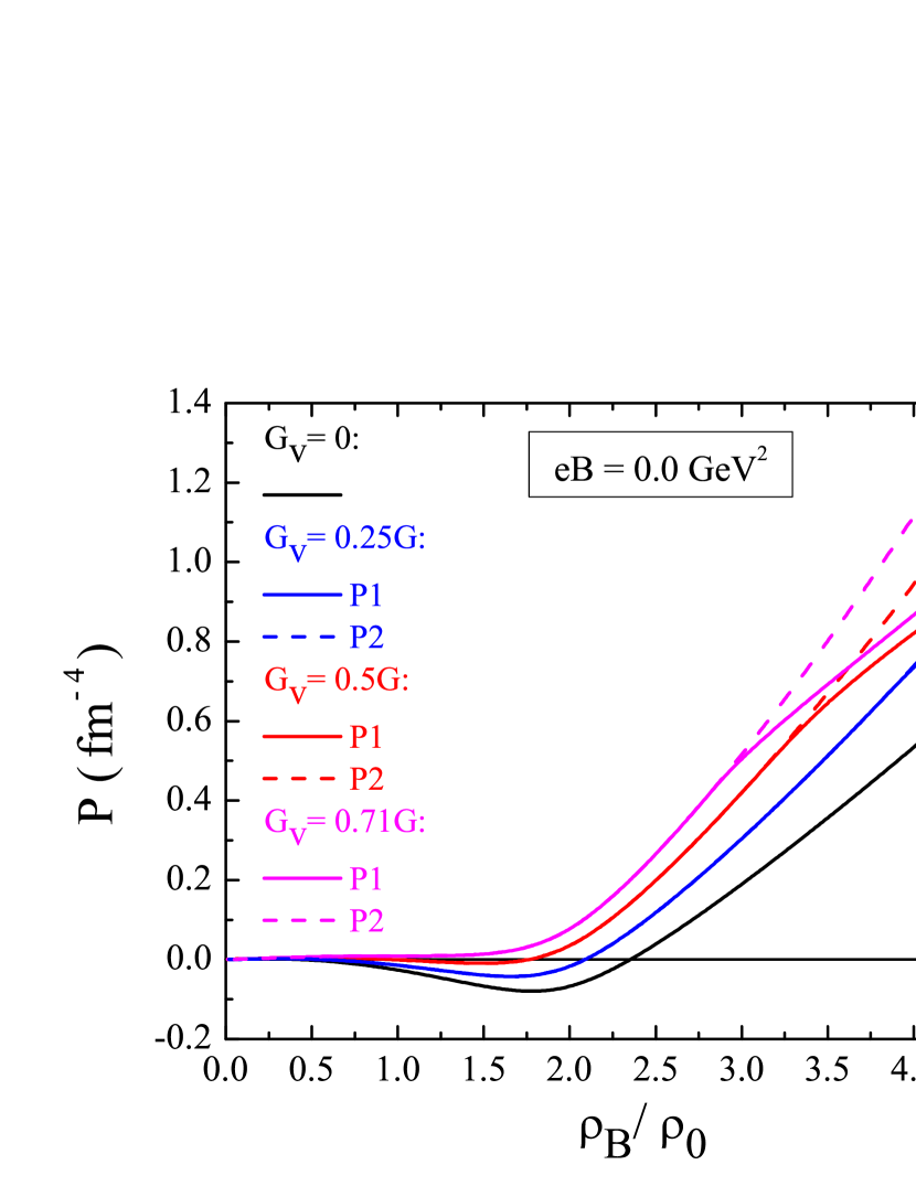
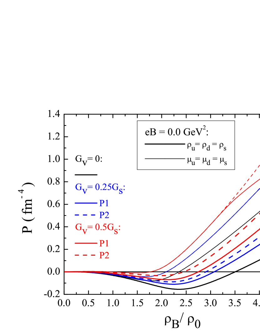
Figure 1: The pressure versus baryonic density for model 1 (P1) and 2 (P2) for different values of $x$ and parametrization RKH, under the conditions a) $\mu_{u}=\mu_{d}=\mu_{s}$, b) $\rho_{u}=\rho_{d}=\rho_{s}$ (thick lines) and $\mu_{u}=\mu_{d}=\mu_{s}$ (thin lines).

The effect on the EOS of the different forms for the vector interaction is seen in Fig. 1a), where the parametrization RKH is used with different strengths of the vector interaction, for both P1 and P2 under the equal chemical potentials constraint. Several conclusions are in order: a) the models coincide until $\sim 3-4\rho_{0}$, where $\rho_{0}=0.17$ fm^-3 is the nuclear matter saturation density, depending on the magnitude of $x$. The larger $x$ the earlier the two models differ. This is due to the onset of the strangeness that occurs at smaller densities with form P1 as is shown latter; b) once the strangeness sets on the EOS becomes softer, therefore, for large enough densities P1 is softer than P2; c) the pressure is negative for some values of $G_{V}$, including $G_{V}=0$, a feature observed and discussed in hanauske , with consequences on possible coexisting phases and associated phase transition; d) for a large enough $G_{V}$ the first order phase transition observed for densities below 2$\rho_{0}$ disappears, and the pressure increases monotonically with the baryonic density. For the parametrization RKH this occurs for $x=0.71$ and is represented by the pink curves in the figure.

In Fig. 1b), we compare two different scenarios, $\mu_{u}=\mu_{d}=\mu_{s}$ and $\rho_{u}=\rho_{d}=\rho_{s}$ represented, respectively, by the thin and thick lines. The equal flavor densities, corresponding to matter generally designated by strange quark matter, is softer, gives rise to a larger density discontinuity at the first order phase transition. In this scenario the EOS for models P1 and P2 differ for all baryonic densities because the vector interaction form given in Eq. (6) results in different contributions in each case. This scenario may be approximately realized at the center of a quark star.

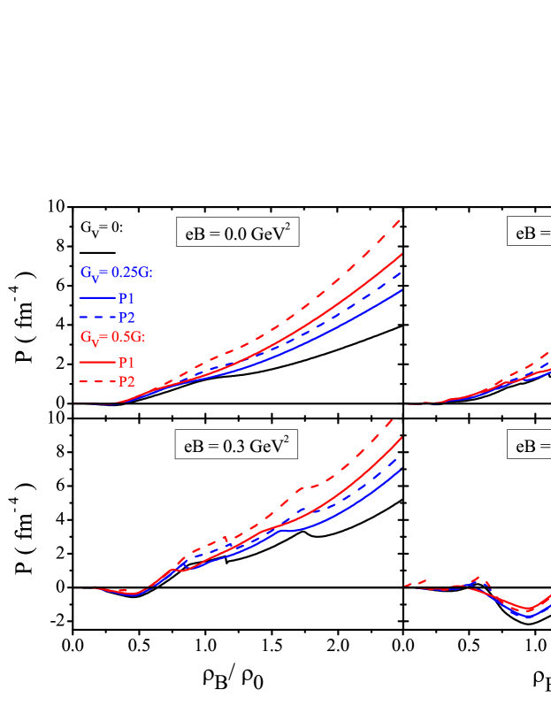
Figure 2: Pressure versus baryonic density for equal chemical potentials and models P1 and P2 for different values of x, and several intensities of the magnetic field: $eB=0$, $eB=0.1$ GeV², $eB=0.3$ GeV² and $eB=0.6$ GeV².

The effect of the magnetic field on the EOS is seen comparing the four graphs of Fig. 2. We first discuss the scenario $\mu_{u}=\mu_{d}=\mu_{s}$. We have chosen three values of $eB$, 0.1, 0.3 and 0.6 GeV² corresponding to $5m_{\pi}^{2}$, $15m_{\pi}^{2}$ and $30m_{\pi}^{2}$. The van-Alphen oscillations due to the filling of the Landau levels are already seen for $eB=0.1$ GeV². The EOS becomes harder at large densities, and the larger $eB$ the harder the EOS, although locally, when the filling of a new Landau level begins, the EOS becomes softer. This increased softness is immediately overtaken by an extra hardness. The larger $B$ the larger the amplitude of the fluctuations and the smaller the number of them, because less Landau levels are involved. The softening occurring when a new Landau level starts being occupied has a strong effect at the smaller densities giving rise to a pressure that is negative within a larger range of densities. For $eB=0.3$ GeV², a magnetic field that could occur at LHC experiments, negative pressures occur beyond $\rho_{B}=0.5$ fm^-3 and this range increases until $\sim 1-1.5$fm^-3 for $eB=0.6$ GeV². The vector interaction P2 gives always the hardest EOS due to the smaller strangeness content.

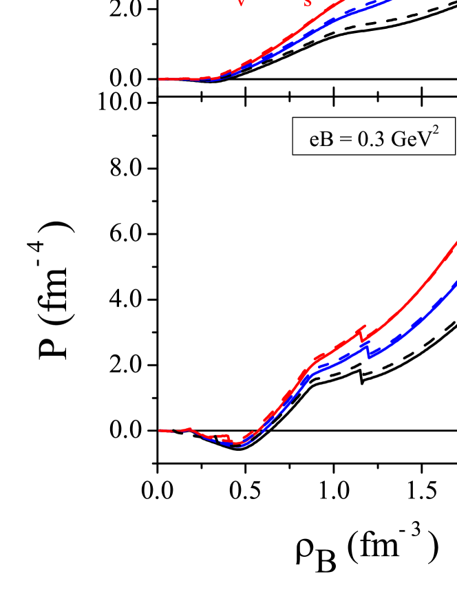
Figure 3: Pressure versus baryonic density for model 2 (P2) for different values of $x$. Two parametrizations of the NJL are compared HK and RKH with magnetic field intensities: a) $eB=0$; b) $eB=0.3$ GeV².

In Fig. 3 the EOS obtained with interaction P2 and the two different parametrizations of the NJL model are compared for $eB$=0 and 0.3 GeV². For $G_{V}=0$ the EOS obtained with the HK parametrization does not cross the RKH EOS. This is no longer valid for a finite $G_{V}$. The RKH EOS becomes stiffer and the two EOS cross within the range of densities shown in the figure. This feature is still present for a finite magnetic field (see Fig. 3b).

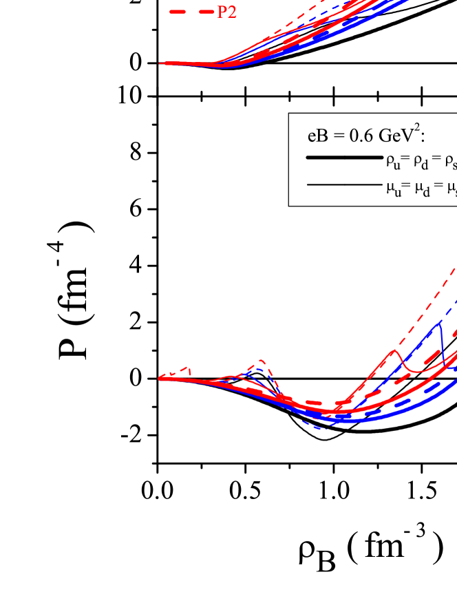
Figure 4: Pressure versus baryonic density for models P1 and P2 for equal quark densities, different values of $x$ for: a) $eB=0$; b) $eB=0.6$ GeV².

Now we move to the scenario of equal flavor densities. The EOS are plotted in Fig. 4 for $eB=0$ and $0.6$ GeV². As already referred before, this scenario is softer than the equal chemical potentials one for the range of densities shown. However, at sufficiently large densities both scenarios converge. In fact, above chiral symmetry restoration it is expected that equal chemical potentials correspond to equal densities. The effect of a strong magnetic field is very different in both scenarios: while the equal chemical potentials EOS presents very strong oscillations, these are not seen for the scenario of equal densities. In the equal chemical potentials the $s$-quark density remains zero until a quite high baryonic density, and, therefore, for a given density below the strangeness onset the $u$ and $d$-quark densities are much larger than in the equal quark densities. Larger $u$ and $d$ quark densities give rise to the restoration of chiral symmetry at lower baryonic densities. Since the effect of the magnetic field is stronger the smaller the masses, this explains the differences in the bottom graphs of Fig. 4 between the two scenarios.

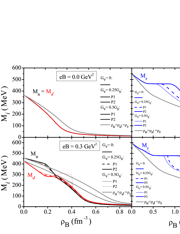
Figure 5: The quark constituent masses as a function of the baryonic density for models P1 and P2, different values of $x$ for $eB=0$ (top figures) and $eB=0.3$ GeV² (bottom figures).

The difference between the chiral symmetry restoration in the two scenarios presented above is clearly seen in Fig. 5, where the constituent masses of the $u$, $d$, and $s$ quarks are plotted for different strengths of the vector interaction and the two models P1 and P2. We first comment on the $eB=0$ results and the two vector interactions, top panels of Fig. 5. The chiral restoration of $u$ and $d$ quarks does not depend on the interaction. However, a difference is observed between the equal chemical potentials and equal densities scenarios.

In the scenario of equal densities (gray lines), one can see that the chiral symmetry restoration of the $u$ and $d$ quarks occurs at larger densities than in the situation with equal chemical potentials (red lines) because the $u$ and $d$ quark densities are larger in the last situation. For the $s$ quark, the opposite occurs. Including the vector interaction does not affect the quark masses in model P2, but it does affect the $s$ quark mass in model P1. In this case the larger $G_{V}$ the faster the chiral restoration of the $s$-quark mass, due to the larger $s$-quark density. At finite $B$ similar conclusions are drawn, but also new aspects arise. First of all the constituent masses of $u$ and $d$ quarks do not coincide anymore due to the charge difference. Since the $u$ quark has a larger charge, $M_{u}>M_{d}$ in the scenario of equal densities. In the scenario of equal chemical potentials there is a competition between the effect of the charge and the effect of density. For the larger magnetic field considered discontinuities are obtained. These correspond to first order phase transitions associated to the filling of the Landau levels.

The above results on the constituent quark masses confirm that the large oscillations of the EOS seen in Fig. 4b) for the equal chemical potentials is in fact due to the small masses of the $u$ and $d$ quarks.

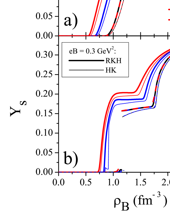
Figure 6: The strangeness fraction as a function of the baryonic density for models P1 and P2 and different values of $G_{V}$, and a) $B=0$; b) $eB=0.3$ GeV².

It is interesting to compare the strangeness content of matter under the conditions discussed until this point. We next analyze once more the situation of equal chemical potentials. In Fig. 6 the strange quark fraction for P1 and P2 models, three values of $G_{V}$, and $eB=0$ and 0.3 GeV² are displayed. We also report results for the parametrizations RKH (thick) and HK (thin). One aspect that is immediately observed is that the P2 model presents the least amount of strange quarks, and its content does not depend on $G_{V}$, both for zero and a finite magnetic field. However, the P1 model does affect the strange quark content and the larger $G_{V}$ the earlier is the onset of the $s$-quark, and the larger its content. One should notice that the definition of the effective chemical potentials in equations (8) and (11) is directly reflected on the strangeness content. The magnetic field does not erase this feature. Nevertheless, the filling of new Landau levels decreases the rate of the increase of the $s$-quark content as observed in Fig. 6b). Parametrizations RKH and HK behave in a similar way with RKH predicting an onset of $s$-quarks at smaller densities, and a larger amount of strangeness for a given baryonic density.

III.2 Stellar matter: quark stars

We next move to the study of stellar matter, i.e., matter where $\beta$-equilibrium and charge neutrality are enforced. In this case, leptons are introduced in the system, so that equations

$$\mu_{s}=\mu_{d}=\mu_{u}+\mu_{e},\qquad\mu_{e}=\mu_{\mu}.$$ (13)

and

$$\rho_{e}+\rho_{\mu}=\frac{1}{3}(2\rho_{u}-\rho_{d}-\rho_{s}).$$ (14)

are satisfied.

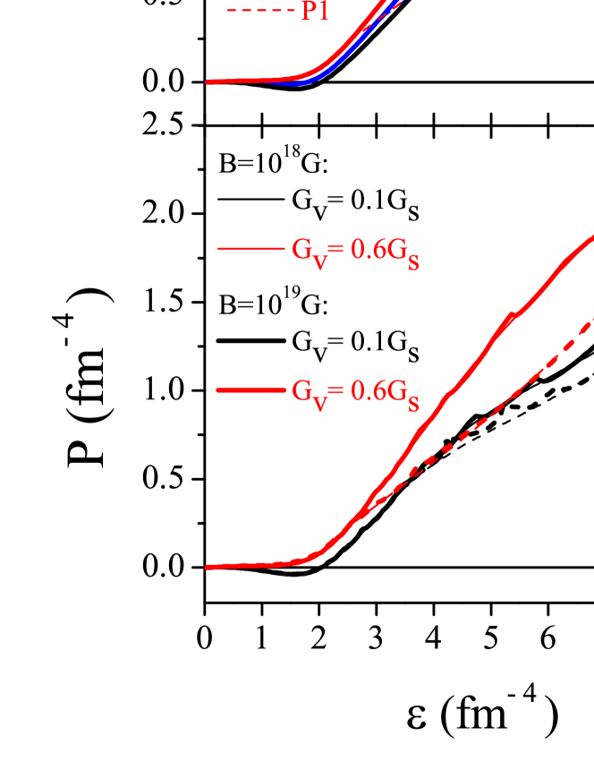
Figure 7: The pressure versus energy density (EOS) for model P1 (thin lines) and P2 (thick lines) for different values of $G_{V}$ and a) $B=0$; b) $B=10^{18}$ and $10^{19}$ G. Both figures were obtained for the parametrization RKH.

Since, to date, there is no information available on the star interior magnetic field, we assume that the magnetic field is baryon density-dependent as suggested in chakra97 . In the following we consider a magnetic field that increases with density according to

$$B=B_{surf}+B_{0}(1-\exp[-\beta{(\rho/\rho_{0})}^{\gamma}]),\quad\beta=0.02,\,\gamma=3,$$ (15)

$B_{surf}=10^{15}$ G is the magnetic field at the surface of the star. As our aim in this section is to compare results with astrophysical observations, the use of magnetic fields in Gauss units is more adequate. We have considered that $eB=1$ GeV² corresponds to $B=1.685\times 10^{20}$ G. In the following we start by investigating the effects of the vector interaction in stellar matter applied do quark stars and subsequently we choose the best possible model and parameter set to build hybrid stars and look at their macroscopic properties.

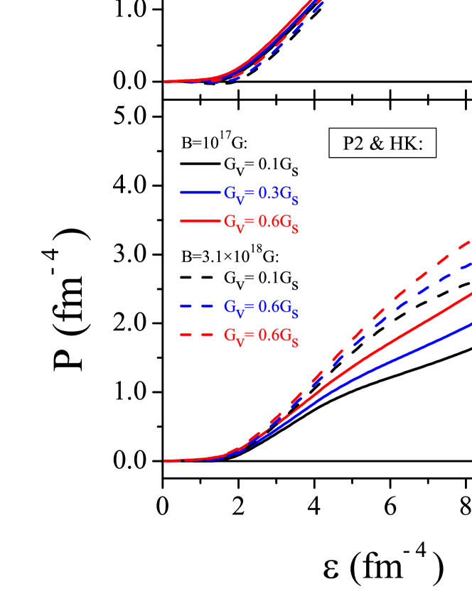
Figure 8: EOS for model 2 (P2) for different values of $G_{V}$, and a) $B=3.1\times B=10^{18}$ G obtained with parametrizations HK and RKH and b) two intensities of the magnetic field: $B=10^{17}$ G and $B=3.1\times 10^{18}$ G for parameter set HK.

Once again, we start from the non-magnetized case and check the differences arising from both models with the RKH parameter set and different values of $G_{V}$ in Fig. 7. The same conclusions reached from the pure quark matter case can be drawn here, mainly that P2 gives rise to a harder EOS and that at very low energy densities, the pressure becomes slightly negative. This difference can be easily understood if one looks at Eqs. (7) and (9), from where it is seen that the contribution from the vector term to the pressure is larger in model P2 because in this case it is flavor blind. The effect of the magnetic field on the quark matter is stronger for the large densities when the magnetic field is more intense due to the density dependence we have considered, see Eq. (15), and much larger when we consider $B_{0}=10^{19}$ G. The fluctuations arising due to the filling of new Landau levels seem larger and more frequent for the smaller vector coupling on an energy density versus pressure curve. This arises because for a stronger vector term a larger energy density is obtained for the same density, and therefore, the fluctuations are spread over a larger energy density range.

We then reobtain the EOS for the cases where $B=10^{17}$ and $3.1\times 10^{18}$ G. These values were chosen as the limiting ones because below $B=10^{17}$ G, all EOS coincide with the non-magnetized case and $3.1\times 10^{18}$ G is the maximum value that allows us to avoid anisotropic pressures veronica . This is also the maximum intensity supported by a star bound by the gravitational interaction before the star becomes unstable lai91 . However, as we are using a density dependent magnetic field, this value may be never reached in the star core.

In Fig.8a), we compare both parametrizations for a fixed magnetic field equal to $3.1\times 10^{18}$ G and different values of $G_{V}$. We can observe that HK yields harder EOS than RKH. The van Alphen oscillations are noticeable for this field intensity. The feature of HK and RKH EOS crossing with the increase of the vector interaction, observed when pure quark matter is analyzed, occurs at energy densities larger than the ones shown in the figure. In Fig. 8b), we fix the HK parametrization and plot the EOS for the two intensities of the magnetic field mentioned above. It is interesting to observe that at large densities an EOS obtained with a smaller magnetic field becomes harder for certain values of $G_{V}$ than an EOS obtained with a much stronger magnetic field and a smaller value of $G_{V}$.

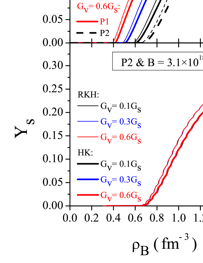
Figure 9: Strangeness fraction as a function of the baryonic density for $B=0$, parameter sets HK and RKH a) for models 1 (P1) and 2 (P2) and different values of $x$ and b) model 2 (P2) for different values of $x$ with $B=3.1\times 10^{18}$ G.

			HK			RKH
			$x=0.1$	$x=0.3$	$x=0.6$	$x=0.1$	$x=0.3$	$x=0.6$
$B=0$ G	P1	$M_{max}$ ($M_{0}$)	1.49	1.58	1.69	1.27	1.35	1.46
		R (km)	9.13	10.89	11.98	8.01	8.17	9.41
		$\varepsilon_{c}$ ($\mathrm{fm}^{-4}$)	7.23	6.96	6.52	9.42	9.61	9.84
	P2	$M_{max}$ ($M_{0}$)	1.56	1.72	1.91	1.35	1.54	1.74
		R (km)	9.15	10.61	11.47	8.22	8.60	9.91
		$\varepsilon_{c}$ ($\mathrm{fm}^{-4}$)	7.35	7.37	6.92	8.71	8.58	8.09
$B=10^{17}$ G		$M_{max}$ ($M_{0}$)	1.56	1.72	1.91	1.35	1.54	1.74
P2		R (km)	9.16	10.16	10.95	8.21	8.58	9.60
		$\varepsilon_{c}$ ($\mathrm{fm}^{-4}$)	7.41	7.36	6.98	8.80	8.94	8.11
$B=3.1\times 10^{18}$ G		$M_{max}$ ($M_{0}$)	1.96	2.03	2.12	1.81	1.88	1.98
P2		R (km)	9.98	10.43	11.05	9.03	9.21	9.90
		$\varepsilon_{c}$ ($\mathrm{fm}^{-4}$)	7.41	7.22	6.78	8.74	8.21	7.80

Table 2: Stellar macroscopic properties obtained from EOS of non-magnetized matter for models P1 and P2 and for magnetized matter with model P2 and two values of magnetic field intensities. $M_{max}$ is the maximum mass, R is the star radius and $\varepsilon$ the star central energy density.

We proceed to the analysis of the strangeness content for non-magnetized matter, whose curves are depicted in Fig. 9a). As in the case of pure quark matter, the amount of strange quarks remains unchanged with any variation of $G_{V}$ with model P2 while it increases with the increase of $G_{V}$ if model P1 is used. RKH presents higher strangeness content than HK with consequences in the maximum stellar masses, as we show next. For the sake of completeness, we show the strangeness fraction for $B=3.1\times 10^{18}$ G and the two parameter sets discussed in the present work in Fig. 9b) for the strangeness blind vector interaction P2. As already expected from the softness of the EOS, we see that HK introduces a smaller strangeness content in the system and if we compare the values obtained with different values of the magnetic field ranging from $B=10^{17}$ G to $B=3.1\times 10^{18}$ G, we can see that the amount of strange quarks remains practically unaltered for both parameter sets.

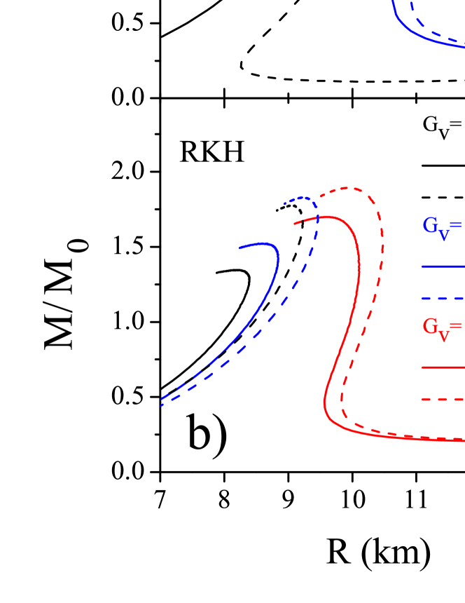
Figure 10: Mass radius curves obtained with model 2 (P2) for different values of $G_{V}$, two intensities of the magnetic field ($B=10^{17}$ G and $B=3.1\times 10^{18}$ G) and parametrizations a) HK and b) RKH.

Finally, we use the EOS discussed above as input to the Tolman-Oppenheimer-Volkoff equations tov and show our results in Fig. 10 and Table 2. A general trend is that HK, being harder with less strange quarks, produces higher maximum masses. A not so common feature is that for some combination of $G_{V}$ values and magnetic field intensities, the quark stars behave as hadronic stars in the sense that the densities attained at low pressure are indeed very small. This is seen in Fig. 10 in all cases where the low mass stars have very large radii. This feature has already been observed in Ref.hanauske for non-magnetized stars and it is related to the existence/non existence of negative pressures at very low densities for small/large values of the vector interaction coupling.

We see that the maximum masses obtained with zero and low magnetic field intensities ($B=10^{17}$ G) are always coincident, but the radii are slightly different due to the small differences in the central energy densities. Within RKH the most massive neutron stars have less $\sim 0.2\,M_{\odot}$ than if the HK parametrization is used. HK can reach quite high maximum mass values, of the order of 2 $M_{\odot}$, for either large values of the vector interaction even with low or zero magnetic fields or for high magnetic fields and any value of the vector interaction. Concerning the radii, some comments are in order: in Hebeler , the radii of the canonical $1.4\,M_{\odot}$ neutron star was estimated to lie in the range 9.7-13.9 Km. More recently, there was a prediction that they should lie in the range $R=9.1^{+1,3}_{-1.5}$ Km guillot and another one stating that the range should be $10-13.1$ Km Lattimer2013 . From Fig. 10, one can see that there is a window of values for $G_{V}$ and $B$ which result in radii accepted by any of the above mentioned analyzes.

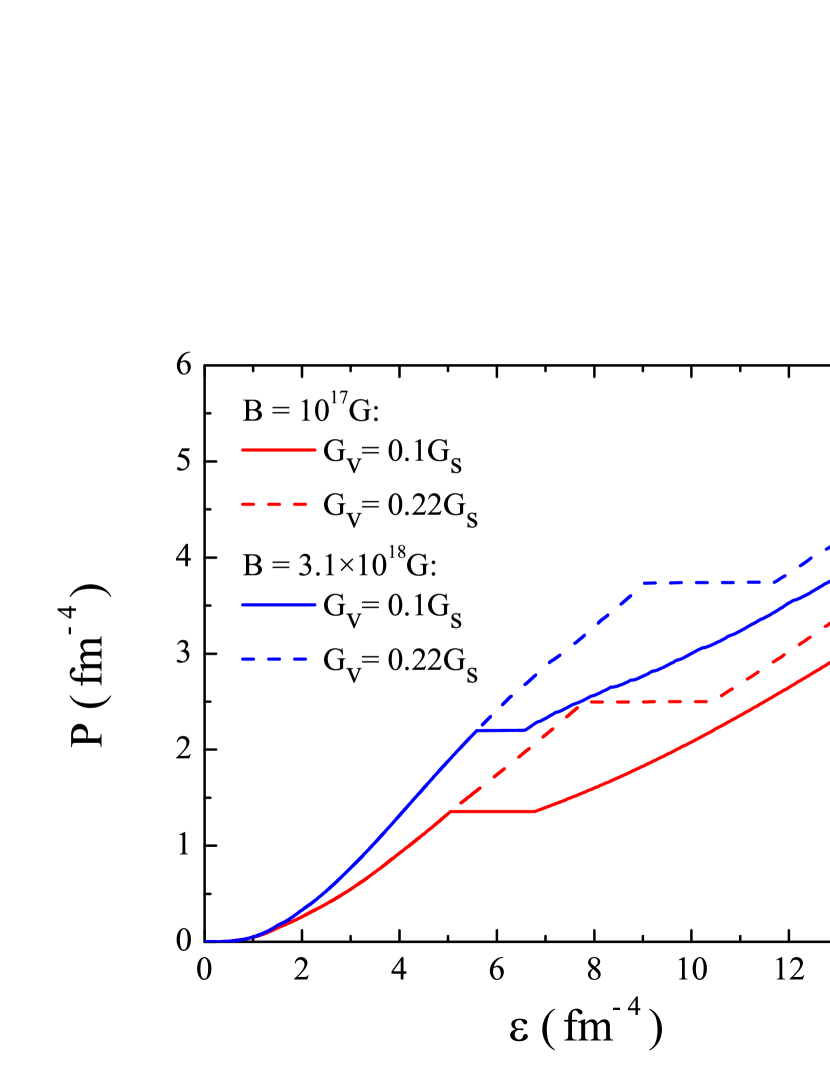
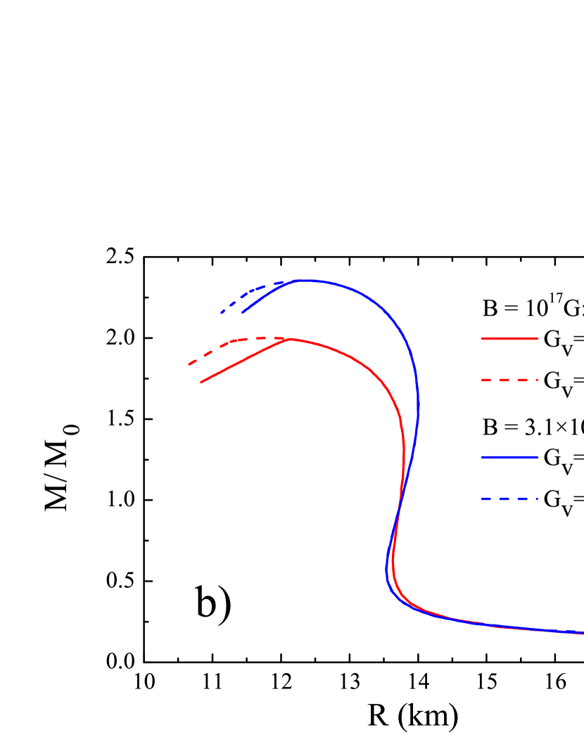
Figure 11: Hybrid star - a) EOS and b) Mass radius curves obtained with model 2 (P2) for different values of $G_{V}$, two intensities of the magnetic field ( $B=10^{17}$ G and $B=3.1\times 10^{18}$ G) and parametrization HK.

III.3 Stellar matter: hybrid stars

To make our analysis of the vector interaction as broad as possible, we dedicate this subsection to revisit the case of hybrid stars under the influence of strong magnetic fields. We study the structure of hybrid stars based on the Maxwell condition (without a mixed phase), where the hadron phase is described by the GM1 GM1 parametrization of the non-linear Walecka model Serot and the quark phase by the NJL model with the inclusion of the vector interaction as discussed in the previous subsection. As stated in the Introduction, hybrid stars have already been extensively discussed for the non-magnetized case pagliara ; bonanno ; lenzi2012 ; logoteta ; shao2013 ; sasaki2013 ; masuda2013 . For the possible existence of magnetars that can be described by hybrid stars, the reader can refer to panda and hybrid and we refrain from writing the mathematical expressions here.

HK		$M_{max}$	$M_{b}$	R	$\varepsilon_{c}$	$\varepsilon$ (onset)	$\rho_{c}$	$\rho$ (onset)	$\mu_{B}(\varepsilon_{c})$	$\mu_{B}$ (onset)
		($M_{0}$)	($M_{0}$)	(km)	($\mathrm{fm}^{-4}$)	($\mathrm{fm}^{-4}$)			(MeV)	(MeV)
$B=10^{17}$ G	$x=0$	1.91	2.18	12.78	4.57	3.47	0.78	0.62	1360	1330
P2	$x=0.10$	1.99	2.30	12.14	6.27	5.05	-	0.84	-	1503
	$x=0.22$	2.00	2.31	11.82	5.93	7.79	0.95	1.18	1580	1726
$B=3.1\times 10^{18}$ G	$x=0$	2.27	2.60	12.82	4.69	3.30	0.70	0.54	1324	1261
P2	$x=0.10$	2.35	2.70	12.34	5.29	5.59	0.74	0.78	1427	1453
	$x=0.22$	2.35	2.70	12.35	5.27	9.03	0.74	1.18	1426	1730
RKH		$M_{max}$	$M_{b}$	R	$\varepsilon_{c}$	$\varepsilon$ (onset)	$\rho_{c}$	$\rho$ (onset)	$\mu_{B}(\varepsilon_{c})$	$\mu_{B}$ (onset)
		($M_{0}$)	($M_{0}$)	(km)	($\mathrm{fm}^{-4}$)	($\mathrm{fm}^{-4}$)			(MeV)	(MeV)
$B=10^{17}$ G	$x=0$	1.97	2.26	12.48	4.29	4.28	-	0.74	-	1422
P2	$x=0.10$	2.00	2.31	11.91	7.51	5.67	-	0.92	-	1557
	$x=0.19$	2.00	2.31	11.83	5.91	7.83	0.95	1.18	1579	1728
$B=3.1\times 10^{18}$ G	$x=0$	2.33	2.69	12.79	4.69	4.19	-	0.63	-	1335
P2	$x=0.10$	2.35	2.70	12.34	5.30	6.52	0.74	0.88	1428	1531
	$x=0.19$	2.35	2.70	12.34	5.30	9.05	0.74	1.18	1428	1731

Table 3: Stellar macroscopic properties obtained from EOS of magnetized hybrid stars built with GM1 and SU(3) NJL with HK and RKH parametrizations. $M_{max}$ is the maximum gravitational mass, $M_{b}$ is the maximum baryonic mass, $R$ is the star radius, $\varepsilon_{c}$ is the star central energy density, $\mu_{B}(\varepsilon_{c})$ is the chemical potential for neutron at $\varepsilon_{c}$ and $\mu_{B}$(onset) is the baryonic chemical potential at the onset of the quark phase.

In face of the results we have obtained for quark stars, we next choose to construct hybrid stars with the P2 model and both HK and RKH parameter sets because this vector interaction term yields the hardest quark matter EOS. For the hadronic phase, we use the GM1 parametrization GM1 and hyperon meson coupling constants equal to fractions of those of the nucleons, so that $g_{iH}=X_{iH}g_{iN}$, where the values of $X_{iH}$ are chosen as $X_{\sigma H}=0.700$ and $X_{\omega H}=X_{\rho H}=0.783$ glen . This is the same choice as in hybrid for the case of hybrid stars with the quark phase described by the NJL model (without the vector interaction). The EOS obtained with a Maxwell construction for magnetic fields equal to $B=10^{17}$ G and $B=3.1\times 10^{18}$ G are shown in Fig.11a) for two values of $x$, being $x=0.22$ the maximum possible value for which a hybrid star can be built with parameter set HK. For values larger than 0.22, the quark matter EOS becomes too hard and in a pressure versus baryonic chemical potential, the hadronic and quark EOS no longer cross each other. For an EOS built with GM1 and RKH, the curves are very similar, but the maximum possible value of $x$ for the crossing of the hadronic and the quark EOS is 0.19.

Taking into account that NJL does not describe the confinement feature of QCD, we cannot, in fact, fix the low-density normalization of the pressure. In order to account for this uncertainty the authors of pagliara ; lenzi2012 ; bonanno ; logoteta have included an extra bag pressure that allows the density at which the transition to deconfinement occurs vary. Including this term in such a way that the deconfinement transition occurs at lower densities than the ones obtained in the present study would have allowed us to choose a larger $G_{V}$ and therefore, a larger maximum mass would be possible. In the present study we renormalize the pressure in such a way that it is zero for zero baryonic density and do not discuss the effect of including an extra bag pressure.

In Fig. 11b) the mass radius curves obtained for the HK parametrization from the solution of the TOV equations are displayed. These macroscopic results are also shown in Table 3. In this table we present results for both the HK and RKH parametrizations, three values of the vector couplings, $x=0,\,0.1,$ and the maximum possible value of $x$ for each parameter set, and two values of the magnetic field intensity $B=10^{17}$ and $3.1\times 10^{18}$ G. Some of the entrances for the central baryonic density are not indicated because they lie on an intermediate value between the density of the hadronic phase at the quark phase onset and the corresponding density of the quark phase. The only maximum mass configuration that really has a quark core is obtained for $B=10^{17}$ G and $G_{V}=0$ within the HK parametrization, giving rise to a 1.91 $M_{\odot}$ star. It is worth pointing out that the largest maximum masses are now obtained, in general, with the parameter set RKH and not HK, the case of quark stars. This is due to the fact that the quark phase sets in at smaller densities for the HK parametrization making the EOS softer. This result had already been obtained in hybrid ; paoli .

One can see that the maximum stellar masses depend very little on the vector interaction strength. For the larger magnetic field considered, the onset of quark matter occurs at a larger density than the central density of the maximum mass hadronic star configuration, for both parametrizations. The same occurs for $B=10^{17}$ G and $G_{V}=0.22$ ($G_{V}=0.19$) for the HK (RKH) parameter set. In these cases the properties of the quark phase do not affect the star properties. On the order hand, from Fig. 11b) for $B=10^{17}$ G and $G_{V}=0.1$, it seems that as soon as the quark phase sets in the star becomes unstable. Nevertheless, if we compare the baryonic density at the centre of the star with the baryonic density at the onset of quarks, we conclude that this maximum mass star could, in principle, contain a quark core. Had we performed a Gibbs construction, the star core would be in a mixed phase. All other stars are ordinary hadronic stars.

As an overall conclusion, it may be stated that a star that is subject to a strong magnetic field attains a smaller baryonic density in its centre, and, therefore, the quark phase is not favored. This same conclusion was obtained in panda where the quark phase was described within the MIT bag model. Moreover, since the inclusion of a vector interaction makes the quark EOS harder, it is also natural to expect that a quark EOS with a large $G_{V}$ difficults the occurrence of a quark core. The weak point of the standard NJL model is the fact that it does not include confinement, and, therefore, the normalization considered for the pressure is not well defined.

Stars with very high masses are predicted and maximum masses of observed compact stars may set an upper limit for the largest possible magnetic field at the centre of the star, ∼$2\times 10^{18}$ G for 2$M_{\odot}$ stars.

Of course, had we chosen the P1 model to build the hybrid star, the $x$ value that would allow for a Maxwell construction would certainly be larger than 0.19 or 0.22, depending on the choice of parameters, but the stellar maximum mass would probably be smaller than 2 $M_{\odot}$. It is worth remembering that all results presented here depend also on the choice of the coupling constants and meson-hyperon parameters for the hadron phase.

IV Final remarks

In the present work we have studied quark matter in the presence of a strong magnetic field. We had as our main objective understanding the interplay between the effects of an external magnetic field effect and the presence of vector interaction in the quark density Lagrangian. Quark matter was described within the SU(3) NJL model, and we have considered two forms of the vector interaction, a flavor dependent and a flavor independent ones, both frequently used in the literature.

Two scenarios of homogeneous quark matter were considered: equal flavor chemical potential and equal flavor density. In the first scenario the role of the vector interaction is an important ingredient, affecting the fraction of each kind of quarks. For the flavor dependent vector interaction the $s$ quark fraction increases with the vector interaction. Within the flavor independent vector interaction the strangeness sets in at a quite high baryonic density independently of the vector coupling. As the presence of $s$ quarks softens the EOS, the hardest EOS were obtained with the flavor independent vector interaction. The larger the vector coupling the harder the EOS. At low densities the magnetic field has an effect contrary to the vector interaction and softens the EOS due to appearance of Landau levels with a large degeneracy. In fact, if the vector interaction is strong enough the low density first order transition disappears and a crossover occurs. The magnetic field, however, increases the range of densities for which matter is unstable. On the other hand, at large densities, both the vector interaction and the magnetic field act in the same direction, in particular, they make the EOS harder.

Stellar matter and compact star properties in the presence of a static magnetic field that increases with the baryonic density, have also been studied. For quark stars we have shown that the larger the vector coupling the larger the maximum star mass, independently of the form of the vector interaction. Moreover, it was shown that the flavor independent vector interaction predicts larger mass stars, which can be 0.1- 0.3 $M_{\odot}$ larger depending on the magnitude of the vector interaction. The presence of a static magnetic field increases the maximum mass, and masses above $\sim 2M_{\odot}$ are obtained for a magnetic field that is $\sim 3\times 10^{18}$ G in the centre of the star.

We have shown that within the present quark model hybrid stars with a quark content in its centre are only possible if neither the vector coupling nor the magnetic fields are too strong. Strong magnetic fields disfavor the formation of a quark phase. This fact, however, may have interesting consequences as already discussed in panda , giving rise to a phase transition when the magnetic field decays. This kind of phase transitions are expected to release a large amount of energy, possibly in the form of a $\gamma$-ray burst.

V Acknowledgements

This work was partially supported by CNPq (Brazil), CAPES (Brazil) and FAPESC (Brazil) under project 2716/2012,TR 2012000344, by COMPETE/FEDER and FCT (Portugal) under Grant No. PTDC/FIS/113292/2009 and by NEW COMPSTAR, a COST initiative.

References

- (1) B.D.Serot and J.D. Walecka, Advances in Nuclear Physics, Vol. 16, eds. J.W. Negele and E. Vogt (Plenum, New York, 1986).
- (2) V. Koch, T.S. Biro, J. Kunz and U. Mosel, Phys. Lett. B 185, 1 (1987).
- (3) H. Abuki, R. Gatto and M. Ruggieri, Phys. Rev. D 80, 074019 (2009)
- (4) J. Xu, T. Song, C.M. Ko and F. Li, Phys. Rev. Lett. 112, 012301 (2014).
- (5) K. Fukushima, Phys. Rev. D 78, 114019 (2008).
- (6) S. Klimt, M. Lutz, and W. Weise, Phys. Lett. B 249, 386 (1990).
- (7) M. Hanauske, L. M. Satarov, I. N. Mishustin, H. Stöcker, and W. Greiner, Phys. Rev. D 64, 043005 (2001).
- (8) J.-L. Kneur, M.B. Pinto and R.O. Ramos, Phys. Rev. C 81, 065205 (2010).
- (9) G. Pagliara and J. Schaffner-Bielich, Phys. Rev. D 77, 063004 (2008).
- (10) L. Bonanno and A. Sedrakian, Astronomy & Astrophysics 539, A16 (2012).
- (11) C. Lenzi and G. Lugones, Astrophys. J. 759, 57 (2012).
- (12) D. Logoteta, C. Providência and I. Vidaña, Phys. Rev. C 88, 055802 (2013).
- (13) G.Y. Shao, M. Colonna, M. Di Toro, Y.X. Liu and B. Liu, Phys. Rev. D 87, 096012 (2013).
- (14) T. Sasaki, N. Yasutake, M. Kohno, H. Kouno and M. Yahiro, arXiv: 1307.0681[hep-ph].
- (15) K. Masuda, T. Hatsuda and T. Takatsuda, Prog. Ther. Exp. Phys. 2013, 073D01 (2013).
- (16) K. Fukushima, D. E. Kharzeev and H. J. Warringa, Phys. Rev. D 78, 074033 (2008); D. E. Kharzeev, L.D. McLerran and H. J. Warringa, Nucl. Phys. A 803, 227 (2008); D. E. Kharzeev and H. J. Warringa, Phys. Rev. D 80, 0304028 (2009); D. E. Kharzeev, Nucl. Phys. A 830, 543c (2009).
- (17) K. Tuchin, Adv. High Energy Phys. 2013, 490495 (2013).
- (18) R. Duncan and C. Thompson, Astrophys. J. Lett. 392, L9 (1992); C. Kouveliotou et al., Nature 393, 235 (1998).
- (19) O. Scavenius, Á. Mócsy, I.N. Mishustin and D.H. Rischke, Phys. Rev. C 64, 045202 (2001).
- (20) S.S. Avancini, D.P. Menezes, M.B. Pinto and C. Providência, Phys. Rev. D 85, 091901 (2012).
- (21) P. Costa, M. Ferreira, H. Hansen, D.P. Menezes and C. Providência, Phys. Rev. D (2014), in press; arXiv:1307.7894[hep-ph].
- (22) T. Inagaki, D. Kimura and T. Murata, Prog. of Theo. Phys. 111, 371 (2004).
- (23) F. Preis, A. Rebhan and A. Schmitt, JHEP 1103, 033 (2011).
- (24) R.O. Ramos and P.H.A. Manso, Phys. Rev. D 87, 125014 (2013); J.-L. Kneur, M.B. Pinto and R.O. Ramos, Phys. Rev. D 88, 045005 (2013).
- (25) F. Preis, A. Rebhan and A. Schmitt, Lect. Notes Phys. 871, 51 (2013).
- (26) D. Ebert, K.G. Klimenko, M.A. Vdovichenko and A. S. Vshivtsev, Phys. Rev. D 61, 025005 (2000); P.G. Allen and N. N. Scoccola, Phys. Rev. D 88, 094005 (2013); A. G. Grunfeld, D. P. Menezes, M.B. Pinto and N.N. Scoccola, arXiv:1402.4731 [hep-ph].
- (27) R.Z. Denke and M.B. Pinto, Phys. Rev. D 88, 056008 (2013).
- (28) T. Hatsuda and T. Kunihiro, Phys. Rep. 247, 221 (1994).
- (29) P. Rehberg, S. P. Klevansky and J. Hüfner, Phys. Rev. C 53, 410 (1996).
- (30) P. B. Demorest, T. Pennucci, S. M. Ransom, H. S. E. Roberts, J. W. T. Hessel, Nature 467, 1081 (2010).
- (31) Antoniadis, J.; Freire, P. C. C.; Wex, N.; Tauris,T. M.; Lynch, R. S.; Van Kerkwijk, M. H.; Kramer, M.; Bassa, C. et al., Science 340, 1233232 (2013).
- (32) M. Buballa, Phys. Rept. 407, 205 (2005).
- (33) O. Lourenço, M. Dutra, T. Frederico, A. Delfino and M. Malheiro, Phys. Rev. D 85, 097504 (2012).
- (34) T-G Lee, Y. Tsue, J. Providência, C. Providência and M. Yamamura, Prog. Ther. Exp. Phys. 2013, 013D02 (2013).
- (35) K. Fukushima, Phys. Rev. D 77, 114028 (2008).
- (36) N.M. Bratovic, T. Hatsuda and W. Weise, Phys. Lett. B 719, 131 (2013).
- (37) D.P. Menezes, M. Benghi Pinto, S.S. Avancini, A. Pérez Martinez and C. Providência, Phys. Rev. C 79, 035807 (2009).
- (38) S.S. Avancini, D.P. Menezes, M.B. Pinto and C. Providência, Phys. Rev. C 80, 065805 (2009).
- (39) D. Bandyopadhyay, S. Chakrabarty and S. Pal, Phys. Rev. Lett. 79, 2176 (1997).
- (40) V. Dexheimer, D.P. Menezes and M. Strickland, J. Phys G: Nucl. Part. Phys. 41, 015203 (2014).
- (41) D. Lai and S. Shapiro, Astrophys. J. 383, 745 (1991).
- (42) R.C. Tolman, Phys. Rev. 55, 364 (1939); J.R. Oppenheimer and G.M. Volkoff, Phys. Rev. 55, 374 (1939).
- (43) K. Hebeler, J. M. Lattimer, C. J. Pethick and A. Schwenk, Phys. Rev. Lett. 105, 161102 (2010).
- (44) S. Guillot, M. Servillat, N. A. Webb and R. E. Rutledge, ApJ 772, 7 (2013).
- (45) J. M. Lattimer and A. W. Steiner, arXiv:1305.3242 [astro-ph.HE].
- (46) M. K. Glendenning and S.A. Moszkowski, Phys. Rev. Lett. 67, 2414 (1991).
- (47) B. D. Serot, J. D. Walecka, Adv. Nucl. Phys. 16, 1 (1986).
- (48) A. Rabhi, H. Pais, P. K. Panda and C. Providência, J. Phys. G: Nucl. Part. Phys. 36, 115204 (2009).
- (49) R. Casali, L.B. Castro and D.P. Menezes, Phys. Rev. C 89, 015805 (2014).
- (50) N. K. Glendenning, Compact Stars, Springer, New York (2000).
- (51) M.G. Paoli and D.P. Menezes, Europ. Phys. J. A 46, 413 (2010).