Holographic thermalization patterns

Abstract:

We investigate the behaviour of various correlators in $\mathcal{N}=4$ super Yang Mills theory, taking finite coupling corrections into account. In the thermal limit we investigate the flow of the quasinormal modes as a function of the ’t Hooft coupling. Then by using a specific model of holographic thermalization we investigate the deviation of the spectral densities from their thermal limit in an out-of-equilibrium situation. The main focus lies on the thermalization pattern with which the various plasma constituents of different energies approach their final thermal distribution as the coupling constant decreases from the infinite coupling limit. All results point towards the weakening of the usual top down thermalization pattern.

1 Introduction

Understanding the processes behind the complicated field dynamics in a relativistic heavy ion collision presents a complicated challenge to QCD theorists. Experiments at RHIC and the LHC, together with the early onset of hydrodynamical behaviour, indicate that the produced state of matter behaves as a strongly coupled ideal fluid with very low shear viscosity over entropy ratio. The strongly coupled nature of the quark gluon plasma (QGP) has led the gauge/gravity duality to become one of the standard tools to investigate its properties [1, 2]. The duality has proven particularly useful in investigating time dependent out-of-equilibrium phenomena and the approach to thermal equilibrium by mapping the strongly coupled field dynamics to black hole formation in asymptotically anti-deSitter (AdS) space time in one higher dimension. This has led to the insight that the early applicability of hydrodynamics, sometimes called hydroization or hydrodynamization, does not mean that the system is isotropic, let alone thermal.

Another important question in a thermalizing system concerns the thermalization pattern with which the plasma constituents of different energies approach their final thermal distribution. On the weakly coupled side classical calculations have shown that the thermalization process is of the bottom-up type, i.e. low energetic modes reach their thermal distribution first, with inelastic scattering processes being the driving mechanism behind it [3]. In the early stages of the collision many soft gluons are emitted which form a thermal bath rather quickly, which then draws energy from the hard modes. Recently this picture got supported by numerical simulations [4]. In [5] an alternative proposal was made: the thermalization process is driven by instabilities which isotropize the momentum distributions more rapidly than scattering processes. On the contrary, holographic calculations in the infinite coupling limit always point towards top-down thermalization where the high energetic modes reach thermal equilibrium first, indicating a probable transition at intermediate coupling.

In this proceedings we are going to investigate the thermalization patterns in $\mathcal{N}=4$ super-Yang Mills (SYM) plasma and its dependence on the coupling constant. This is done through the determination of the off-equilibrium retarded Greens functions whose evolution gives direct information about how plasma constituents of different energies approach their thermal distribution. On the one hand we will investigate the plasma constituents themselves by looking at energy momentum tensor correlators [6]. On the other hand we will also use photons as probes for the thermalization process, which provide an observational window into the thermalization process, because once emitted they stream through the plasma almost unaltered [8, 7, 9, 10].

2 The setup

2.1 the collapsing shell model

We work within one of the simplest models of holographic thermalization, using the radial collapse of a spherical shell of matter and the subsequent formation of a black hole [11]. Due to Birkhoff’s theorem, outside the shell the metric is given by a black hole solution, whereas inside it is given by its zero temperature counterpart

$$ds^{2}=\frac{r_{h}^{2}}{L^{2}u}\left[f(u)dt^{2}+dx^{2}+dy^{2}+dz^{2}\right]+\frac{L^{2}}{4u^{2}f(u)}du^{2}\;,$$ (1)

where

$$f(u)\,=\,\left\{\begin{array}[]{lr}f_{+}(u)=1-u^{2}\,,&\mathrm{for}\;u>u_{s}\\ f_{-}(u)=1\,,&\mathrm{for}\;u<u_{s}\end{array}\right.\;,$$ (2)

and $u\equiv r_{h}^{2}/r^{2}$ is a dimensionless coordinate where the boundary is located at $u=0$ and the horizon at $u=1$. From now on the index ’–’ denotes the inside and ’+’ the outside space-time of the shell and we set the curvature radius of the $AdS$ space to $L=1$.

The shell can be described by the action for a membrane

$$S_{m}=-p\int d^{4}\sigma\sqrt{-\det g_{ij}}\;,$$ (3)

where $g_{ij}$ is the induced metric on the brane and $p$ is the only parameter that characterizes the membrane. Due to the discontinuity of the time coordinate, fields living in the above background have to be matched across the shell using the Israel matching conditions given by

$$[K_{ij}]=\frac{\kappa_{5}^{2}p}{3}g_{ij}\;,$$ (4)

where $[K_{ij}]=K^{+}_{ij}-K^{-}_{ij}$ is the extrinsic curvature and $\kappa_{5}$ denotes the gravitational constant. From the above equation the trajectory of the shell is determined. We however are not going to treat the full dynamical process but work in the quasi static approximation, where the motion of the shell is slow compared to the other scales of interest and take snapshots at different positions of the shell . In the quasi static approximation the matching conditions for the different fields $\phi_{i}$ we are considering simplify considerably and can be written in the uniform way [13]

$$\phi_{i}^{-}|_{u_{s}}=\sqrt{f_{s}}\phi_{i}^{+}|_{u_{s}},\qquad\partial_{u}\phi_{i}^{-}+\frac{\kappa_{5}^{2}p}{3u}\phi_{i}^{-}|_{u_{s}}=f_{s}\partial_{u}\phi_{i}^{+}|_{u_{s}}\;.$$ (5)

In what follows we set $\kappa_{5}^{2}p=1$, which was set to zero in previous studies for photons [8, 7, 9, 10].

2.2 Finite coupling corrections

In order to go beyond the usual $\lambda=\infty$ limit the type IIB supergravity action has to be supplemented by the first order string corrections of order $\alpha^{\prime 3}$ in the inverse string tension [14]

$$S_{\mathrm{IIB}}=\frac{1}{2\kappa_{10}}\int d^{10}x\sqrt{-g}\left[R_{10}-\frac{1}{2}(\partial\varphi)^{2}-\frac{1}{4.5!}(F_{5})^{2}\,+\gamma\;e^{\frac{-3}{2}}\varphi\Big{(}C+\mathcal{T}\Big{)}^{4}\right]\;.$$ (6)

$R_{10}$ denotes the Ricci scalar, $\gamma\equiv\frac{1}{8}\zeta(3)\lambda^{-\frac{3}{2}}$, $\varphi$ the dilaton field and $F_{5}$ the five-form field strength, while $C$ stands for the Weyl tensor and the tensor ${\mathcal{T}}$ is given by

$$\mathcal{T}_{abcdef}=i\nabla_{a}F^{+}_{bcdef}+\frac{1}{16}\left(F^{+}_{abcmn}F_{def}^{+\;\;mn}-3F^{+}_{abfmn}F_{dec}^{+\;\;mn}\right)\,.$$ (7)

The index triplets $\{a,b,c\}$ and $\{d,e,f\}$ are understood to be first antisymmetrized with respect to all permutations, and the two triplets then symmetrized with respect to the interchange $abc\leftrightarrow def$. One should also note that our notation for the various contractions in equ. (6) is only schematic, and e.g. the $C^{4}$ term in fact denotes the combination

$$C_{hmnk}C_{pmnq}C_{h}^{\;rsp}C^{q}_{\;rsk}+\frac{1}{2}C^{hkmn}C_{pqmn}C_{h}^{\;rsp}C^{q}_{\;rsk}\,.$$ (8)

For further details of this construction, see e.g. [15] and references therein.

From the above action the $\gamma$-corrected metric is obtained from which one can then obtain the $\gamma$-corrected equations of motion (EoM) for a transverse U(1) vector field $E$ and metric perturbations of the form $g_{\mu\nu}\rightarrow g_{\mu\nu}+h_{\mu\nu}$.

Following [16] the metric perturbations can be combined into three gauge invariant fields $Z_{i}$ representing the three symmetry channels, namely the spin 0 (sound channel), spin 1 (shear channel) and the spin 2 (scalar channel). The EoMs are solved using standard AdS/CFT techniques. However, due to the presence of the shell the outside solution is a linear combination of the ingoing and outgoing modes, ($\phi_{a}={E,Z_{i}}$),

$$\phi_{a}^{+}=c_{+}\phi_{a,in}+c_{-}\phi_{a,out}.$$ (9)

where the coefficients $c_{\pm}$ are solved from the matching conditions (5). The spectral densities of the electric field and the gauge invariants are obtained from

$$\chi_{E}(\omega,q,u_{s},\gamma)=\frac{N_{c}^{2}T^{2}}{2}\mathrm{Im}\left[\frac{E^{\prime}_{+}(u)}{E_{+}(u)}\right],\qquad\chi_{Z_{i}}(\omega,q,u_{s},\gamma)=\frac{N_{c}^{2}T^{4}}{2}\mathrm{Im}\left[\frac{Z^{\prime\prime}_{i,+}(u)}{Z_{i,+}(u)}\right]\Bigg{|}_{u=0}$$ (10)

which need to be expanded to linear order in $\gamma$. For the thermalization processes it is useful to study the relative deviation of the spectral densities from their thermal limit (denoted by ’th’ below)

$$R_{a}(\omega,q,u_{s}\gamma)=\frac{\chi_{a}(\omega,q,u_{s}\gamma)-\chi_{\mathrm{a,th}}(\omega,q,\gamma)}{\chi_{a,\mathrm{th}}(\omega,q,\gamma)}\,.$$ (11)

3 Results

Having outlined the main steps of our computation, we will now present the results, which are divided into two parts. We start from the thermal limit and inspect the effect of infinitesimal perturbations on the system by solving the quasinormal mode (QNM) spectrum and by analyzing the flow of the poles as functions of $\lambda$. Then we use the collapsing shell model to study the behaviour of various spectral densities and their approach to thermal equilibrium taking the leading order string corrections into account. In the case of photons we also study the virtuality dependence.

3.1 Quasi normal modes

Quasinormal modes characterize the response of the system to infinitesimal external perturbations and are the strong coupling equivalent to the quasiparticle picture of the weakly coupled field theory. They are solutions to linearized fluctuations of some bulk field obeying incoming boundary conditions at the horizon and Dirichlet boundary conditions at the boundary. They appear as poles of the corresponding retarded Green’s function and have the generic form

$$\omega_{n}(q)=M_{n}(q)-i\Gamma_{n}(q),$$ (12)

where $q$ is the three momentum of the mode, $M_{n}$ and $\Gamma_{n}$ correspond to the mass and the decay rate of the excitation, respectively.

        

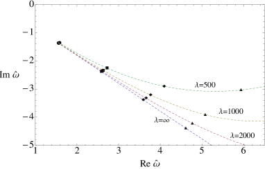
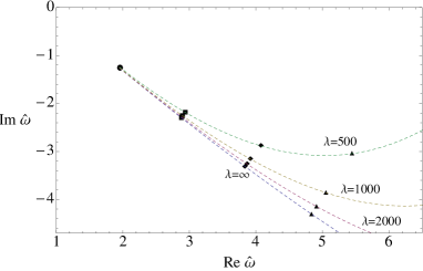
Figure 1: The flow of the QNM in the scalar channel for $q=0$ (left) and $q=2\pi T$ (right) as a function of $\lambda$. The dashed lines are drawn to illustrate the bending of the tower of QNM towards the real axis as the coupling constant decreases.

In fig. 1 we show the flow of the tower of QNM obtained from the photon and scalar channel correlator. In both cases a clear trend is visible. As the coupling constant is decreased from the infinite coupling limit the imaginary part of $\omega_{n}$ increases rapidly. Also note that higher energetic modes show a stronger dependence on the coupling constant, with a larger shift towards the real axis. From equ.(12) one deduces that finite coupling corrections extend the lifetimes of the excitations. It should be noted though that the strong coupling expansion can only be trusted when the deviation from the infinite coupling limit is small, which clearly is not the case for all displayed poles.

3.2 Thermalization of the spectral density

In order to study the thermalization pattern of the different plasma constituents it is most instructive to look at the relative deviation of the spectral density from its thermal limit given in (11). Starting with the infinite coupling limit we display in fig. 3 how the relative deviation of the scalar channel behaves for different positions of the shell. As the shell moves towards the horizon the amplitude of $R$ decreases while the frequency increases, showing that the system thermalizes. From this figure one can also see that high energetic modes are closer to equilibrium than the low energetic ones, showing the usual top-down thermalization pattern. The same conclusion holds for all other modes as well, and in the case of photons an analytic calculation [10] reveals that $R\sim 1/\omega$.

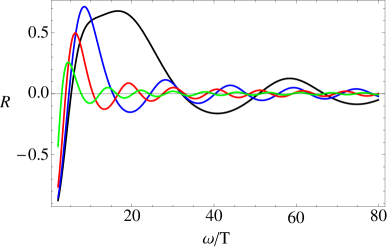
Figure 2: R in the scalar channel using $q=0$ and $\lambda=\infty$ for $u_{s}=0.1,\;0,4,\;0.7,\;0.9$ (from large to small amplitudes).

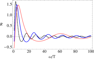
Figure 3: R for photons for different virtualities $c=1,\;0.8,\;0$ (from large to small amplitudes) for $u_{s}=0.6$.

As a next step we look at the virtuality dependence of $R$ in the $\lambda=\infty$ case by letting the virtuality $v=(\omega^{2}-q^{2})/\omega^{2}$ be a free parameter. We parameterize $q=c\omega$ and plot in fig. 3 the relative deviation, $R$, for $c=0$, 0.8 and 1. The most important effect of the virtuality is that the larger the virtuality of the photon is, the smaller is the amplitude of the oscillations. This implies that on shell photons are last to thermalize while maximal virtual photons, i.e. dileptons at rest, thermalize first.

        

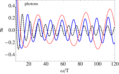
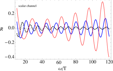
Figure 4: Left: The relative deviation $R$ photons for $\lambda=100$ and $u_{s}=0.8$ and different values of $c=1,\;0.8,\;0$ (from large to small amplitudes). Right: The same values as before in the scalar channel but for $c=8/9,\;6/9,\;0$ (from large to small amplitudes). The rise of R at some critical value points towards a weakening of the usual top down thermalization pattern.

We are now ready to move on and study finite coupling effects on the the relative deviation of the spectral density, shown in fig. 4 for photons and the scalar channel for three different values of $c$ at a fixed position of the shell and $\lambda=100$. For small frequencies the usual top down pattern persists, which however changes for larger values of $\omega/T$. For $c=0$, the relative deviation approaches a constant. As $c$ is increased $R$ starts to rise again at some critical value. First of all this shows that finite coupling corrections have a larger impact on the high energetic modes, in accordance with the QNM analysis. Second, at large frequencies the relative deviation strongly depends on the value of $c$ (in the case of photons on the virtuality). The larger the value of $c$ the bigger is the deviation from the thermal limit. We interpret this as a weakening of the usual top-down thermalization pattern moving towards bottom-up at smaller coupling.

4 Conclusions

In the paper at hand we studied holographic thermalization patterns of $\mathcal{N}=4$ SYM theory and their dependence on the coupling constant. First, we investigated the flow of the tower of QNM as a function of the ’t Hooft coupling. As the coupling decreases from the infinite coupling limit the imaginary part of the quasinormal modes increases, extending the lifetime of the excitation. Higher energetic modes show a stronger dependence on the finite coupling corrections. This analysis is particularly useful since it is independent of the thermalization model being used.

Second, we analyzed the relative deviation of spectral densities from their thermal limit using the collapse of a thin shell of matter and the subsequent formation of a black hole working within the quasi static approximation. At infinite coupling the usual top-down pattern is observed. In the case of photons there is a strong dependence on the virtuality. On shell photons are last to thermalize, whereas dileptons at rest thermalize first.

Going away from the infinite coupling limit changes the top-down pattern. At a critical value of the frequency the relative deviation starts rising again, being further away from its equilibrium value compared to smaller frequencies. All observed behaviours point towards that the usual top-down thermalization pattern at infinite coupling moves towards bottom-up as the coupling constant decreases. The effect of finite coupling corrections on thermalizing geometric probes can be found in [17].

References

- [1] O. DeWolfe, S. S. Gubser, C. Rosen and D. Teaney, arXiv:1304.7794.
- [2] J. Casalderrey-Solana, H. Liu, D. Mateos, K. Rajagopal and U. Wiedemann, arXiv:1101.0618.
- [3] R. Baier, A. H. Mueller, D. Schiff and D. T. Son, Phys. Lett. B 502 (2001) 51
- [4] J. Berges, K. Boguslavski, S. Schlichting and R. Venugopalan, arXiv:1303.5650.
- [5] A. Kurkela and G. D. Moore, JHEP 1112 (2011) 044
- [6] S. A. Stricker, arXiv:1307.2736.
- [7] R. Baier, S. A. Stricker, O. Taanila and A. Vuorinen, JHEP 1207 (2012) 094
- [8] R. Baier, S. A. Stricker, O. Taanila and A. Vuorinen, Phys. Rev. D 86 (2012) 081901
- [9] D. Steineder, S. A. Stricker and A. Vuorinen, Phys. Rev. Lett. 110 (2013) 101601
- [10] D. Steineder, S. A. Stricker and A. Vuorinen, JHEP 1307 (2013) 014
- [11] U. H. Danielsson, E. Keski-Vakkuri and M. Kruczenski, Nucl. Phys. B 563 (1999) 279
- [12] S. Lin and H. -U. Yee, Phys. Rev. D 88 (2013) 025030
- [13] S. Lin and E. Shuryak, Phys. Rev. D 78 (2008) 125018
- [14] M. F. Paulos, JHEP 0810 (2008) 047
- [15] B. Hassanain and M. Schvellinger, JHEP 1212 (2012) 095
- [16] P. K. Kovtun and A. O. Starinets, Phys. Rev. D 72 (2005) 086009
- [17] W. H. Baron and M. Schvellinger, JHEP 1308 (2013) 035