Optimal interval clustering: Application to Bregman clustering and statistical mixture learning

Abstract

We present a generic dynamic programming method to compute the optimal clustering of $n$ scalar elements into $k$ pairwise disjoint intervals. This case includes 1D Euclidean $k$-means, $k$-medoids, $k$-medians, $k$-centers, etc. We extend the method to incorporate cluster size constraints and show how to choose the appropriate $k$ by model selection. Finally, we illustrate and refine the method on two case studies: Bregman clustering and statistical mixture learning maximizing the complete likelihood.

Key words: Clustering, dynamic programming, $k$-means, Bregman divergences, statistical mixtures, exponential families.

1 Introduction

Clustering is a fundamental and key primitive to discover structural groups of homogeneous data, called clusters, in data sets. The most famous clustering technique is the celebrated $k$-means [1] that seeks to minimize the sum of intra-cluster variances by prescribing beforehand the number of clusters, $k$. On one hand, solving the $k$-means problem is NP-hard [7] when the dimension $d>1$ and $k>1$ and various heuristics locally optimizing the $k$-means objective function like Lloyd’s batched $k$-means [1] have been proposed. When $d>1$ and $k>1$, NP-hardness also holds for other clustering problems like $k$-medoids, $k$-medians and $k$-centers [10]. On the other hand, it is well-known that those center-based clustering problems are fully characterized when $k=1$: For example, the centroid [1] is the solution of the $1$-mean, the Fermat-Weber point [10] the solution of the geometric $1$-median, the circumcenter [10] the solution of the $1$-center, etc. Surprisingly, it is less known that $k$-means can be solved exactly in 1D by using dynamic programming [2, 15] (DP).

In this letter, we first revisit and extend the seminal dynamic programming (DP) paradigm [2] for optimally clustering $n$ 1D elements into $k$ pairwise disjoint intervals, the clusters. We term clustering with this property: The 1D contiguous or interval clustering problem. We further show how to incorporate constraints on the minimum and the maximum cluster sizes, and perform model selection (i.e., choosing the appropriate $k$) from the DP table. The generic DP solver requires either $O(n^{2}kT_{1}(n))$ time using $O(nk)$ memory or $O(n^{2}T_{1}(n))$ time using $O(n^{2})$ memory, where $T_{1}(n)$ is the time requires for solving the corresponding $1$-cluster problem. Second, we consider two applications that refine the generic DP method: In the first application, we report a $O(n^{2}k)$-time optimal Bregman $k$-means relying on 1D Summed Area Tables [6] (SATs) and also consider the Bregman $\ell_{r}$-clustering problems [9]. In the second application, we consider learning statistical mixture models from independently and identically (iid.) univariate observations by maximizing the complete likelihood: Using the one-to-one mapping between Bregman divergences and exponential families [1], we transform this problem into a series of equivalent 1D Bregman $k$-means clustering that can be solved optimally by DP for statistical mixtures of singly-parametric exponential families (like zero-centered Gaussians, Rayleigh or Poisson families). In the general case, we require that the density graphs intersect pairwise in at most a single point like the Cauchy or Laplacian location families (not belonging to the exponential families) to guarantee optimality.

2 1D contiguous clustering: Interval clustering

Let $\mathbb{X}$ be a one-dimensional space totally ordered with respect to $<$ (usually, $\mathbb{X}=\mathbb{R}$), and $\mathcal{X}=\{x_{1},...,x_{n}\}\subset\mathbb{X}$ a set of $n$ distinct elements. A clustering of $\mathcal{X}$ into $k\in\mathbb{N}$ clusters partitions $\mathcal{X}$ into pairwise disjoint subsets $\mathcal{C}_{1}\subset\mathcal{X},...,\mathcal{C}_{k}\subset\mathcal{X}$ so that $\mathcal{X}=\biguplus_{i=1}^{k}\mathcal{C}_{i}$. Let us preliminary sort $\mathcal{X}$ in $O(n\log n)$ time, so that we assume $x_{1}<...<x_{n}$ in the remainder.

The output of a 1D contiguous clustering is a collection of $k$ intervals $I_{i}=[x_{l_{i}},x_{r_{i}}]$ (such that $\mathcal{C}_{i}=I_{i}\cap\mathcal{X}$) that can be encoded using $k-1$ delimiters $l_{i}$ ($i\in\{2,...,k\}$) since $r_{i}=l_{i+1}-1$ ($i<k$ and $r_{k}=n$) and $l_{1}=1$:

$$\underbrace{[x_{1}...x_{l_{2}-1}]}_{\mathcal{C}_{1}}\ \underbrace{[x_{l_{2}}...x_{l_{3}-1}]}_{\mathcal{C}_{2}}...\underbrace{[x_{l_{k}}...x_{n}]}_{\mathcal{C}_{k}}$$ (1)

To define an optimal clustering among the potential ${{n-1}\choose{k-1}}$ contiguous partitions, we ask to minimize a clustering objective function or energy function:

$$\min_{l_{1}=1<l_{2}<...<l_{k}}e_{k}(\mathcal{X})=\bigoplus_{i=1}^{k}e_{1}(\mathcal{C}_{i}),$$ (2)

where $e_{1}$ denotes the intra-cluster cost and $\oplus$ is a commutative and associative operator for calculating the inter-cluster cost. This framework includes the $k$-means and the $k$-medians ($\bigoplus=\sum$), and the $k$-center [10] ($\bigoplus=\max$) criteria (and their discrete counterparts: $k$-medoids, etc.) among others.

2.1 Solving 1D contiguous clustering using DP

Figure 1: The optimal 1D contiguous clustering is found by dynamic programming by observing that an optimal clustering with $k$ clusters is necessarily found from an optimal clustering with $(k-1)$ clusters (see text and Eq. 3).

Recall that after sorting, we have $x_{1}<...<x_{n}$. Let $\mathcal{X}_{j,i}=\{x_{j},...,x_{i}\}$ ($j\leq i$) and $\mathcal{X}_{i}=\mathcal{X}_{1,i}=\{x_{1},...,x_{i}\}$. We define a $n\times k$ cost matrix $E=[e_{i,j}]$ that stores at entry $(i,m)$ the optimal clustering cost $e_{i,m}=e_{m}(\mathcal{X}_{i})$, where $e_{m}$ is defined using Eq. 2. Similarly, we define a matrix $S=[s_{i,j}]$ of dimension $n\times k$ that stores at position $(i,m)$ the index $j$ of the leftmost point in the $m$-th cluster in ${\mathcal{X}}_{i}$. Therefore the global clustering solution shall be found at entry $(n,k)$ with cost $e_{n,k}=e_{k}(\mathcal{X})$.

To define the optimality equation of dynamic programming, we observe that the optimal solution for a 1D contiguous clustering with $m$ clusters can be defined from the solution of an optimal clustering with $(m-1)$ clusters: Indeed, consider the last cluster interval with left position index $l_{m}$, say $l_{m}=j$, as depicted in Figure 1. Then the clustering of the $(m-1)$ first clusters should be an optimal clustering too: namely, the optimal 1D contiguous clustering with $(m-1)$ clusters on subset $\mathcal{X}_{j-1}$. It follows the following recurrence equation:

$$e_{i,m}=\min_{m\leq j\leq i}\left\{e_{j-1,m-1}\oplus e_{1}(\mathcal{X}_{j,i})\right\},$$ (3)

with $e_{i,1}=e_{1}(\mathcal{X}_{i})$ (note that $e_{m,m}=\bigoplus_{l=1}^{m}e_{1}(\{x_{l}\})$ for $1\leq m\leq k$). We store the argmin of Eq. 3 in matrix $S$ at position $(i,m)$ (entry $s_{i,m}$). We compute the energy matrix $E$ from left to right columns, and from bottom to top lines. This yields a $O(n^{2}kT_{1}(n))$-time DP algorithm using $O(n\times k)$ memory, where $T_{1}(n)$ denotes the time required for computing $e_{1}(\mathcal{X})$: Indeed, each of the $n\times k$ entries of $E$ requires $O(nT_{1}(n))$ time to evaluate Eq. 3.

To recover the optimal clustering, we backtrack the solution in $O(k)$ time from the $S$ matrix storing the left indexes of the last cluster of the best solutions: That is, the left index $l_{k}$ of the $k$-th cluster is stored at $s_{n,k}$: $l_{k}=s_{n,k}$. The cardinality of $\mathcal{C}_{k}$ is $n_{k}=|\mathcal{C}_{k}|=n-l_{k}+1$. Then we iteratively retrieve the previous left interval indexes at entries $l_{j-1}=s_{l_{j}-1,j-1}$ for $j=k-1,...,j=1$ with $n_{j}=|\mathcal{C}_{j}|=r_{j}-l_{j}+1=l_{j+1}-l_{j}$ since $r_{j}=l_{j+1}-1$. Note that $l_{j}-1=n-\sum_{l=j}^{k}n_{l}$ denotes the remaining number of elements to cluster using $(j-1)$ clusters (thus we also have $l_{j}-1=\sum_{l=1}^{j-1}n_{l}$).

Note that when the clustering does not satisfy the 1D contiguous partition property, DP yields anyway a solution that may not be optimal. Furthermore, we may consider adding a weight $w_{i}>0$ to each element $x_{i}\in\mathcal{X}$ (and thus assume the $x_{i}$’s are all distinct).

2.2 Time versus memory optimization

By precomputing all the potential intra-cluster costs $e_{1}(\mathcal{X}_{j,i})$ in $O(n^{2}T_{1}(n))$ time using an auxiliary matrix $E_{1}$ of size $n\times n$, we evaluate Eq. 3 as $e_{i,m}=\min_{m\leq j\leq i}\{e_{j-1,m-1}\oplus E_{1}[j,i]\}$, i.e. in $O(i-m)=O(n)$ time. Matrix $E_{1}$ plays the role of a Look Up Table (LUT), and the time complexity for the DP solver reduces to $O(n^{2}k)$ once the LUT matrix $E_{1}$ has been computed.

Lemma 1

The generic 1D contiguous clustering can be solved optimally using dynamic programming in time $O(n^{2}kT_{1}(n))$ using $O(n\times k)$ memory, or in time $O(n^{2}T_{1}(n))$ time using $O(n^{2})$ memory.

Note that $T_{1}=\Omega(n)$ (in fact, usually, $T_{1}(n)=\Theta(n)$). In Section 3, we will further improve the running time to $O(n^{2}k)$ using $O(nk)$ memory when considering Bregman $k$-means.

2.3 Adding cluster size constraints

Let us add constraints on the sizes of clusters. Let $n_{i}^{-}$ and $n_{i}^{+}$ denote lower and upper bound constraints on the size of the $i$-th cluster $n_{i}=|\mathcal{C}_{i}|$, with $\sum_{l=1}^{k}=n_{i}^{-}\leq n$ and $\sum_{l=1}^{k}=n_{i}^{+}\geq n$. When no constraints are required, we simply add the dummy constraints $n_{i}^{-}=1$ and $n_{i}^{+}=n-k+1$ (all clusters non-empty). In Eq. 3, $j$ range from $m$ to $i$. The $m$-th cluster size $n_{m}=|\mathcal{C}_{m}|=i-j+1$ has to satisfy $n_{m}^{-}\leq n_{m}\leq n_{m}^{+}$. That is, $j\leq i+1-n_{m}^{-}$ and $j\geq i+1-n_{m}^{+}$. Clearly, $j$ has also to be greater than $1+\sum_{l=1}^{m-1}n_{l}^{-}$ (an optimal solution for the constrained optimal $(m-1)$-clustering). It follows, that the optimality equation writes as:

$$e_{i,m}=\mathop{\min_{\max\{1+\sum_{l=1}^{m-1}n_{l}^{-},i+1-n_{m}^{+}\}\leq j}}_{j\leq i+1-n_{m}^{-}}\left\{e_{j-1,m-1}\oplus e_{1}(\mathcal{X}_{j,i})\right\},$$ (4)

For example, a balanced clustering may be obtained by setting $n_{i}^{-}={\lfloor\frac{n}{\lambda k}\rfloor}$ and $n_{i}^{+}={\lceil\frac{\lambda n}{k}\rceil}$ for some $\lambda\in\mathbb{N}$.

2.4 Choosing the appropriate $k$: Model selection

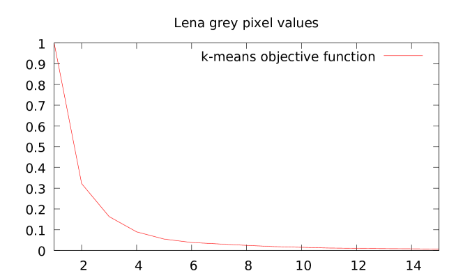
Figure 2: Plot of function $m(k)=e_{k}(\mathcal{X})/e_{1}(\mathcal{X})$ for the optimal $k$-means for $k\in[1,15]$.

The task of clustering data set $\mathcal{X}$ asks also to find the appropriate number of clusters [14]: $k$. Clearly, the more clusters we allow and the less costly the objective function $e_{k}(\mathcal{X})$ is, but the more complex the clustering model to encode. Observe that function $m(k)=\frac{e_{k}(\mathcal{X})}{e_{1}(\mathcal{X})}$ is monotonically decreasing with $k$ and reaches a minimum when $k=n$ (e.g., $0$ for the Euclidean $k$-means) as depicted in Figure 2 (see 4 for an explanation of the data-set). Thus we have to perform some kind of model selection [14] by choosing the best model among all potential models (with number of clusters ranging from $1$ to $n$). The canonical regularized objective clustering cost [14] is $e_{k}^{\prime}(\mathcal{X})=e_{k}(\mathcal{X})+f(k)$ where $f(k)$ is the cost function of choosing a model with $k$ clusters. We can compute the best model minimizing $e_{k}^{\prime}(\mathcal{X})$ by computing for the DP table entries for the last matrix row of $E$ (indexed by $n$, with columns $k$ ranging from $1$ to $n$) the regularized cost. To compute the last row, we iteratively solve DP for $k=n,n-1,...,1$ and avoid redundant computations by checking whether entry $E[i,j]$ has already been computed or not. We then choose $k=\mathrm{argmin}_{g\in\{1,...,k\}}e_{g}^{\prime}(\mathcal{X})$ by scanning the last row with column ranging from $k=1$ to $k=n$.

2.5 A Voronoi condition for optimal center-based clustering

Center-based clustering methods like $k$-means, $k$-medians or $k$-centers store for each cluster $\mathcal{C}_{j}$ a prototype $p_{j}$, the cluster center. For discrete center-based clustering, the prototypes $p_{j}$’s are required to belong to the respective $\mathcal{C}_{j}$’s. The $\ell_{r}$ center-based clustering objective function asks to minimize:

$$\sum_{i=1}^{n}w_{i}\min_{j=1}^{k}d^{r}(x_{i},p_{j})=\sum_{j=1}^{k}\sum_{x_{l}\in\mathcal{C}_{j}}w_{l}d^{r}(x_{l},p_{j}),$$ (5)

where $d(\cdot,\cdot)$ is a dissimilarity measure function (not necessarily a distance). We do not take the $\frac{1}{r}$ power of the sum since it changes the value of $e_{1}$ but not the argmin (prototype). Note that in 1D, $\ell_{s}$-norm distance is always $d_{s}(p,q)=|p-q|$, independent of $s\geq 1$. Thus the intra-cluster cost $e_{1}(\mathcal{C}_{j})$ of a $\ell_{r}$ center-based clustering has to solve the following minimization problem: $e_{1}(\mathcal{C}_{j})=\min_{p_{j}}\sum_{x_{l}\in\mathcal{C}_{j}}w_{l}d^{r}(x_{l},p_{j})$ and retrieve the $j$-th cluster prototype by $p_{j}=\mathrm{argmin}_{p_{j}}\sum_{x_{l}\in\mathcal{C}_{j}}w_{l}d^{r}(x_{l},p_{j})$.

In order for DP to return the optimal clustering, we need to assume that we have the 1D contiguous clustering property. For Euclidean $k$-means, this was proved in [8]. In general, consider the Voronoi cell of prototype $p_{j}$ of $\mathcal{C}_{j}$:

$$V(p_{j})=\{x\in\mathbb{X}\ :\ d^{r}(x,p_{j})\leq d^{r}(x,p_{l})\ \forall l\in\{1,...,k\}\}.$$ (6)

Since $x^{r}$ is a monotonically increasing function on $\mathbb{R}^{+}$, it is equivalent to $V^{\prime}(p_{j})=\{x\in\mathbb{X}\ :\ d(x:p_{j})<d(x:p_{l})\}$. A sufficient condition is to prove that for all potential choices of the $k$ cluster prototypes $\mathcal{P}=\{p_{1},...,p_{k}\}$ the induced 1D dissimilarity Voronoi diagram is made of connected Voronoi cells. A $2$-clustering displays the Voronoi bisector. We now consider two case studies to illustrate and refine the DP method.

3 Optimal 1D Bregman clustering

The $\ell_{r}$-norm Bregman center [9] is defined for $d(p,q)=B_{F}(p:q)$, where $B_{F}(p:q)$ is a univariate Bregman divergence [1]:

$$B_{F}(p:q)=F(p)-F(q)+(p-q)F^{\prime}(q),$$ (7)

induced by a strictly convex and differentiable function $F$. When $F(x)=x^{2}$, we recover the squared Euclidean distance. Bregman divergences are not metric [3], since they violate the triangular inequality and are asymmetric except when $F(x)=\lambda x^{2}$ for $\lambda>0$.

For Bregman $k$-means, the Bregman information [1] of a cluster generalizes the notion of cluster variance. It is the intra-cluster sum of Bregman divergences (Bregman $k$-means, for $r=1$):

$$e_{1}(\mathcal{C}_{j})=\min_{p_{j}}\sum_{x_{l}\in\mathcal{C}_{j}}w_{l}B_{F}(x_{l}:p_{j}).$$ (8)

The cluster prototype [1] is $p_{j}=\frac{1}{\sum_{x_{l}\in\mathcal{C}_{j}}w_{l}}\sum_{x_{l}\in\mathcal{C}_{j}}w_{l}x_{l}$ and the Bregman information is [13]: $e_{1}(\mathcal{C}_{j})=\left(\sum_{x_{l}\in\mathcal{C}_{j}}w_{l}\right)(p_{j}F^{\prime}(p_{j})-F(p_{j}))+\left(\sum_{x_{l}\in\mathcal{C}_{j}}w_{l}F(x_{l})\right)-F^{\prime}(p_{j})\left(\sum_{x\in\mathcal{C}_{j}}w_{l}x\right)$. Observe that the Bregman information relies on three sums $\sum_{x_{l}\in\mathcal{C}_{j}}w_{l}$, $\sum_{x\in\mathcal{C}_{j}}w_{l}x$ and $\sum_{x_{l}\in\mathcal{C}_{j}}w_{l}F(x_{l})$ that can be preprocessed using Summed Area Tables [6] (SATs) since $\mathcal{C}_{j}$ is a contiguous cluster. That is, by computing all the cumulative sums $S_{1}(j)=\sum_{l=1}^{j}w_{l}$, $S_{2}(j)=\sum_{l=1}^{j}w_{l}x_{l}$, and $S_{3}(j)=\sum_{l=1}^{j}w_{l}F(x_{l})$ in $O(n)$ time at preprocessing stage, we can evaluate the Bregman information $e_{1}(\mathcal{X}_{j,i})$ in constant time $O(1)$. For example, $\sum_{l=j}^{i}w_{l}F(x_{l})=S_{3}(i)-S_{3}(j-1)$ with the convention that $S_{3}(0)=0$.

The Voronoi cells of prototypes are defined by $V^{\prime}(p_{j})=\{x\in\mathbb{X}\ :\ B_{F}(x:p_{j})<B_{F}(x:p_{l})\}$. Since Bregman Voronoi diagrams have connected cells [3], it follows that the 1D hard $\ell_{r}$ Bregman clustering satisfies the contiguous interval property, and therefore DP yields the optimal solution. A similar argument directly hold for the Bregman $k$-center that is also the limit case of $\ell_{r}$ Bregman clustering when $p\rightarrow\infty$.

Lemma 2

The 1D $\ell_{r}$ Bregman clustering and Bregman $k$-center can be solved exactly using dynamic programming in $O(n^{2}kT_{1}(n))$ time using $O(n\times k)$ memory, where $T_{1}(n)$ denotes the time to solve the case $k=1$ for $n$ elements. The optimal Bregman $k$-means can be solved in $O(n^{2}k)$ time.

4 Mixture learning by hard clustering

Statistical mixtures are semi-parametric probability models often met in practice. Consider a finite statistical mixture $M$ with $k\in\mathbb{N}$ components. The probability measure $m$ of $M$ with respect to a dominating measure $\nu$ (usually the Lebesgue or counting measure) can be written as:

$$m(x;\Omega)=\sum_{i=1}^{k}\alpha_{i}p(x;\Theta_{i}),x\in\mathbb{X},$$ (9)

with $\alpha=(\alpha_{1},...,\alpha_{k})\in\Delta_{k-1}$ a normalized positive weight vector belonging to the $(k-1)$-dimensional probability simplex, $\Theta=(\Theta_{1},...,\Theta_{k})$, $\Omega=(\alpha,\Theta)$ and $\mathbb{X}$ the support of the distribution. Let $D=\dim(\Theta_{i})\in\mathbb{N}$ denote the number of scalar parameters indexing the probability family $\mathcal{F}=\{p(x;\Theta){\ :\ }\Theta\in\mathbf{\Theta}\}$, called the order. Mixture $m$ is defined by a vector $\Omega\in\mathbf{\Omega}\subseteq\mathbb{R}^{g}$ with $g=k(D+1)-1$, and $\mathbf{\Theta}$ is called the parameter space. Mixtures are inferred from data usually using the Expectation-Maximization algorithm [1]. Since EM locally maximizes the incomplete likelihood [1] and is often trapped into a local maximum, we need some proper mixture parameter initialization or several guided restarts to hopefully reach the optimal solution. On the other hand, maximizing the complete log-likelihood $l_{c}$ for a iid. observation data-set $\mathcal{X}$ amounts to maximize [11]:

$$l_{c}(\mathcal{X};L,\Omega)=\sum_{i=1}^{n}\log(\alpha_{l_{i}}p(x_{i};\theta_{l_{i}})),$$ (10)

where $L=\{l_{i}\}_{i}$ denotes the hidden labels of the $x_{i}$’s. Thus maximizing the complete likelihood is equivalent to minimizing the following objective function:

$$\max l_{c}\equiv\min_{\theta_{1},...,\theta_{k}}\sum_{i=1}^{n}\min_{j=1}^{k}(-\log p(x_{i};\theta_{j})-\log\alpha_{j}).$$ (11)

This is a hard clustering problem for the dissimilarity function $d(x,(\alpha,\theta))=-\log p(x;\theta)-\log\alpha$ (given fixed $\alpha$). As proved in [11], the cluster weights $\alpha_{j}$’s are then updated as the cluster proportion of observations, and the algorithm reiterates by solving Eq. 11. Initially, we choose $\alpha=\frac{1}{k}(1,...,1)$.

Let the additively-weighted minus log-likelihood Voronoi cell be defined by $V(p_{j})=\{x\in\mathbb{X}{\ :\ }-\log p(x;\theta_{j})-\log\alpha_{j}\leq-\log p(x;\theta_{l})-\log\alpha_{l}\}$. In order for DP to return the optimal solution, we need to assert the contiguity property. Using the one-to-one mapping between exponential families [4, 12] and Bregman divergences [1], it turns out that the optimization problem of Eq. 11 yields an equivalent additively-weighted Bregman $k$-means problem (and additively-weighted Bregman Voronoi cells are connected [3]). Thus when the order of the exponential family is $D=1$, we have the contiguity property and DP returns the optimal solution. This works also for curved exponential families with one free parameter like the family of Gaussian distributions $\mathcal{F}=\{N(\mu,\mu^{2})\ :\ \mu\in\mathbb{R}\}$. In general, the contiguity property holds when density graphs in $\mathcal{F}$ are pairwise intersecting at exactly one point of the support $\mathbb{X}$. For example, some (unimodal) location families with density $\mathcal{F}=\{f(x;\mu)=\frac{1}{\sigma}f_{0}(\frac{x-\mu}{\sigma}),\mu\in\mathbb{R}\}$ for a prescribed value of $\sigma>0$ and a standard density $f_{0}(x)$ (e.g., isotropic gaussian densities $N(\mu_{1},\sigma)$ and $N(\mu_{2},\sigma)$ intersect at $x=\frac{\mu_{1}+\mu_{2}}{2}$). This includes location Cauchy distributions and location Laplacian distributions (both not belonging to the exponential families [4]) among others. Note that $1$-order exponential families may have pairwise densities intersecting in more than one point (like the family $\mathcal{F}=\{N(0,\sigma),\sigma\in\mathbb{R}^{+}\}$) but after reparameterization by their sufficient statistic [4] $y_{i}=t(x_{i})$, data-set $\mathcal{Y}=\{y_{i}\}_{i}$ satisfies the contiguous property.

Consider fitting a Gaussian Mixture Model (GMM) on the intensity histogram of the renown lena color image. For each pixel, we compute its grey value and add a small perturbation noise to ensure that we get distinct $x_{i}$’s (alternatively, without adding noise, we set the weight $w_{i}$ of $x_{i}$ as the proportion of pixels having grey value $x_{i}$). We then compute the optimal Euclidean 1D $k$-means for $k=10$ (it corresponds to fitting a 1D GMM $\mathrm{gmm}_{1}$ with Gaussian components having identical standard deviation), and calculate the 1D GMM $\mathrm{gmm}_{2}$ allowing different standard deviations. In that case, we do not have the contiguous clustering property (densities pairwise intersect in two points) and DP may not yield the optimal clustering (give prescribed weights). However, in this case, we experimentally obtained a better GMM. The results are illustrated in Figure 3. For model selection in mixtures, to choose the optimal $k$, we use the Akaike Information Criterion [5] (AIC): $\mathrm{AIC}(x_{1},...,x_{n})=-2l(x_{1},...,x_{n})+2k+\frac{2k(k+1)}{n-k-1}$. Other criteria like the Bayesian Information Criterion (BIC), Minimum Description Length (MDL), etc can also be used.

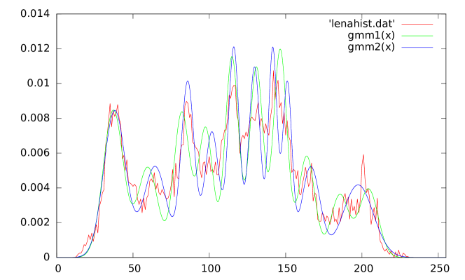
Figure 3: 1D GMMs with $k=10$ components maximizing the complete data likelihood of the intensity histogram of lena image: $\mathrm{gmm}_{1}$ retrieved from an optimal Euclidean $k$-means, and $\mathrm{gmm}_{2}$ allowing different standard deviations. The average complete data log-likelihood of $\mathrm{gmm}_{1}$ is $-3.075$ and that of $\mathrm{gmm}_{2}$ is $-3.039$ (better than the one for $\mathrm{gmm}_{1}$).

5 Conclusion

We first described a clustering algorithm based on dynamic programming (whose seminal idea was briefly outlined in Bellman’s $2$-page paper [2] in 1973) that computes the generic optimal 1D contiguous clustering either in $O(n^{2}kT_{1}(n))$-time using $O(nk)$ memory, or in $O(n^{2}T_{1}(n))$ time using $O(n^{2})$ memory, where $T_{1}(n)$ denotes the time required for solving the case $k=1$ on $n$ scalar elements. We then extended the method to incorporate cluster size constraints and show how to perform model selection from the DP table. This algorithm solves optimally and generically 1D $k$-means, $k$-median and $k$-center among others. Second, we reported two tailored center-based clustering applications of the optimal 1D contiguous clustering: (1) Bregman $k$-means and $k$-centers clustering, and (2) learning statistical mixtures maximizing the complete likelihood provided that (a) their densities belong to a $1$-order exponential family or (b) their density graphs pairwise intersect in one point. For Bregman $k$-means, we showed how to use Summed Area Tables (SATs) to further speed the DP solver in $O(n^{2}k)$-time using $O(nk)$ memory.

References

- [1] Arindam Banerjee, Srujana Merugu, Inderjit S. Dhillon, and Joydeep Ghosh. Clustering with Bregman divergences. Journal of Machine Learning Research, 6:1705–1749, 2005.
- [2] Richard Bellman. A note on cluster analysis and dynamic programming. Mathematical Biosciences, 18(3-4):311 – 312, 1973.
- [3] Jean-Daniel Boissonnat, Frank Nielsen, and Richard Nock. Bregman Voronoi diagrams. Discrete Computational Geometry, 44(2):281–307, September 2010.
- [4] Lawrence D. Brown. Fundamentals of statistical exponential families: with applications in statistical decision theory. Institute of Mathematical Statistics, Hayworth, CA, USA, 1986.
- [5] J. Cavanaugh. Unifying the derivations for the Akaike and corrected Akaike information criteria. Statistics & Probability Letters, 33(2):201–208, April 1997.
- [6] Franklin C. Crow. Summed-area tables for texture mapping. In Proceedings of the 11th Annual Conference on Computer Graphics and Interactive Techniques, SIGGRAPH ’84, pages 207–212, New York, NY, USA, 1984. ACM.
- [7] Sanjoy Dasgupta. The hardness of -means clustering. Technical Report CS2008-0916.
- [8] Walter D Fisher. On grouping for maximum homogeneity. Journal of the American Statistical Association, 53(284):789–798, 1958.
- [9] Meizhu Liu, Baba C. Vemuri, Shun ichi Amari, and Frank Nielsen. Shape retrieval using hierarchical total Bregman soft clustering. IEEE Trans. Pattern Anal. Mach. Intell., 34(12):2407–2419, 2012.
- [10] Nimrod Megiddo and Kenneth J Supowit. On the complexity of some common geometric location problems. SIAM journal on computing, 13(1):182–196, 1984.
- [11] Frank Nielsen. -mle: A fast algorithm for learning statistical mixture models. CoRR, abs/1203.5181, 2012.
- [12] Frank Nielsen and Vincent Garcia. Statistical exponential families: A digest with flash cards, 2009. arXiv.org:0911.4863.
- [13] Frank Nielsen and Richard Nock. Sided and symmetrized Bregman centroids. IEEE Transactions on Information Theory, 55(6):2882–2904, 2009.
- [14] Dan Pelleg and Andrew Moore. -means: Extending -means with efficient estimation of the number of clusters. In Proc. 17th International Conf. on Machine Learning, pages 727–734. Morgan Kaufmann, San Francisco, CA, 2000.
- [15] Haizhou Wang and Mingzhou Song. Ckmeans.1d.dp: Optimal -means clustering in one dimension by dynamic programming. R Journal, 3(2), 2011.