Optimization of mesh hierarchies in Multilevel Monte Carlo samplers

Abstract

We perform a general optimization of the parameters in the Multilevel Monte Carlo (MLMC) discretization hierarchy based on uniform discretization methods with general approximation orders and computational costs. We optimize hierarchies with geometric and non-geometric sequences of mesh sizes and show that geometric hierarchies, when optimized, are nearly optimal and have the same asymptotic computational complexity as non-geometric optimal hierarchies. We discuss how enforcing constraints on parameters of MLMC hierarchies affects the optimality of these hierarchies. These constraints include an upper and a lower bound on the mesh size or enforcing that the number of samples and the number of discretization elements are integers. We also discuss the optimal tolerance splitting between the bias and the statistical error contributions and its asymptotic behavior. To provide numerical grounds for our theoretical results, we apply these optimized hierarchies together with the Continuation MLMC Algorithm haji_CMLMC . The first example considers a three-dimensional elliptic partial differential equation with random inputs. Its space discretization is based on continuous piecewise trilinear finite elements and the corresponding linear system is solved by either a direct or an iterative solver. The second example considers a one-dimensional Itô stochastic differential equation discretized by a Milstein scheme.

1 Introduction

The history of Multilevel Monte Carlo methods can be traced back to Heinrich et al. heinrich98 ; hs99 , where it was introduced in the context of parametric integration. Kebaier kebaier05 then used similar ideas for a two-level Monte Carlo (MC) method to approximate weak solutions to stochastic differential equations (SDEs) in mathematical finance. The basic idea of the two-level MC method is to reduce the number of samples on the fine mesh by using a control variate that is obtained by approximating the solution on a coarser mesh. In giles08 , Giles extended this idea to more than two levels and dubbed his extension the Multilevel Monte Carlo (MLMC) method. Giles introduced a hierarchy of discretizations with geometrically decreasing mesh sizes. His work also included an optimization of the number of samples on each level that reduced the computational complexity to ${\mathcal{O}\left(\mathrm{TOL}^{-2}(\log{\mathrm{TOL}})^{2}\right)}$ when applied to SDEs with Euler-Maruyama discretization, compared to ${\mathcal{O}\left(\mathrm{TOL}^{-3}\right)}$ of the standard Euler-Maruyama MC method. In giles08_m , Giles further reduced the computational complexity of approximating weak solutions of a one-dimensional SDE to ${\mathcal{O}\left(\mathrm{TOL}^{-2}\right)}$ by using the Milstein scheme instead of the Euler-Maruyama scheme to discretize the SDE. MLMC has also been extended and applied in many contexts, including equations with jump diffusions xg12 , partial differential equations (PDEs) with stochastic coefficients bsz11 ; cst13 ; cgst11 ; tsgu13 and stochastic partial differential equations (SPDEs) bls13 ; gr12 , to compute scalar quantities of interest that are functionals of the solutions. In (tsgu13, , Theorem 2.3), an optimal convergence rate is derived for general rates of strong and weak convergence and the computational complexity associated with generating a single sample of the quantity of interest. It is shown that if the strong convergence is sufficiently fast, the computational complexity can be of the optimal rate, ${\mathcal{O}\left(\mathrm{TOL}^{-2}\right)}$.

Several points can be investigated in this standard MLMC setting. For instance, the standard MLMC uses uniform mesh sizes on each level and across the levels the mesh sizes follow a geometric sequence in which the ratio between mesh sizes of subsequent levels is a constant, ${\beta}$, henceforth referred to as level separation. However, it is not clear if this is an optimal choice. Moreover, in the literature, the derivation of the optimal number of samples on each level assumed an equal, fixed splitting of accuracy between statistical and bias error contributions. In haji_CMLMC , the authors used a more efficient splitting that improved the running time of MLMC by a constant factor, but no analysis of the splitting parameter was provided. In this work, we show that, in certain cases, the optimal level separation is not a constant and depends on several parameters, including the level index, $\ell$. Moreover, when restricted to geometric, but not nested, hierarchies, we optimize for the constant level separation parameter, ${\beta}$, by using some heuristics and show that using this optimized value the computational complexity of the geometric hierarchies is close to the computational complexity of the optimized non-geometric hierarchies. We also show that the computational complexity of both hierarchies are the same in the limit as $\mathrm{TOL}\to 0$. In addition, we analyze the optimal splitting parameter, $\theta$, and note its asymptotic behavior as $\mathrm{TOL}\to 0$. Several issues arise in a practical implementation of MLMC. One of these issues is that the hierarchies generated by optimality theorems are usually not applicable due to constraints on either mesh sizes (for instance due to CFL stability limitations) or the number of samples; the constraint on the latter being an integer, for example. We analyze these issues and note their effect on the optimality of the MLMC hierarchies. Other issues include the stopping criteria Bayer2012 and the estimation of variances in the case of a small number of samples, a feature that is inherent to MLMC and is always present in the deepest levels of the MLMC hierarchies. To this end, we here apply these optimized hierarchies together with the Continuation MLMC algorithm (CMLMC) haji_CMLMC and show the effectiveness of the resulting algorithm in several examples. The use of a posteriori error estimates and related adaptive algorithms, as introduced first in hsst12 , is beyond the scope of this work, which focuses instead on optimizing a priori defined parametric families to create the discretization hierarchies.

This work is organized as follows. Section 2.1 recalls the MLMC sampling framework and states the hierarchy optimization problem. Several approximation steps lead to an analytically treatable problem. Section 2.2 presents the solution for the case of unconstrained optimal mesh sizes, including the number of samples per level and the splitting accuracy parameter; these optimal mesh sizes do not form geometric sequences in general. Then, Section 2.3 presents the optimal hierarchies if they are restricted to geometric sequences of mesh sizes. Finally, Section 3 illustrates the theoretical results with numerical examples, which include three-dimensional PDEs with random inputs and Itô SDEs, and Section 4 draws conclusions and proposes future extensions of this work. To avoid cluttering the presentation, the technical derivations of the formulas included in this work are outlined in the appendix.

2 Optimal MLMC hierarchies

Here we state the problem of optimizing the mesh hierarchies in MLMC and present the mesh hierarchies resulting from a theoretical optimization, first allowing very general sequences of mesh sizes and then for comparison restricting ourselves to geometric sequences.

In Section 2.1 we introduce the MLMC hierarchy, the parameters that we consider free to optimize in the hierarchy, and the models of the computational work and of the weak and strong errors that define the general, discrete and non-convex, optimization problem. Simplifying assumptions then lead to an analytically treatable continuous optimization problem in Sections 2.2–2.3.

2.1 Problem setting

Let $g(u)$ denote a scalar quantity of interest, which is a function of the solution $u$ of an underlying stochastic model. Our goal is to approximate the expected value, ${\mathrm{E}\mspace{-2.0mu}\left[g(u)\right]}$, to a given accuracy $\mathrm{TOL}$ with a high probability of success. We assume that individual outcomes of the underlying solution, $u$, and the evaluation of $g(u)$ are approximated by a discretization-based numerical scheme characterized by a mesh size, $h$. The following examples are adapted from haji_CMLMC with some modification:

Example 1

Let $(\Omega,\mathcal{F},\mathbb{P})$ be a complete probability space and $\mathcal{D}$ be a open, bounded and convex polygonal domain in $\mathbb{R}^{d}$. Find $u:\mathcal{D}\times\Omega\to\mathbb{R}$ that solves $\mathbb{P}$-almost surely (a.s.) the following equation:

$$-\nabla\cdot\left(a\nabla u\right) =f, \text{ in }\mathcal{D},$$

$$u =0, \text{ on }\partial\mathcal{D},$$

where the value of the diffusion coefficient and the forcing are represented by random fields, yielding a random solution. We wish to compute ${\mathrm{E}\mspace{-2.0mu}\left[g(u)\right]}$ for some deterministic functional $g$ which is globally Lipschitz satisfying $|g(u)-g(v)|\leq G\|u-v\|_{H^{1}(\mathcal{D})}$ for some constant $G>0$ and all $u,v\in H^{1}(\mathcal{D})$. Following tsgu13 , we also make the following assumptions

• $a_{\min}=\min_{\mathbf{x}\in\mathcal{D}}a(\mathbf{x})>0$ a.s. and $1/a_{\min}\in L^{p}_{\mathbb{P}}(\Omega)$, for all $p\in(0,\infty)$.

• $a\in L^{p}_{\mathbb{P}}(\Omega,C^{1}(\overline{\mathcal{D}}))$, for all $p\in(0,\infty)$.

• $f\in L^{p^{*}}_{\mathbb{P}}(\Omega,L^{2}(\mathcal{D}))$ for some $p^{*}>2$.

Here, $L^{p}_{\mathbb{P}}(\Omega,\mathcal{B})$ is the Bochner space of $p$-th integrable $\mathcal{B}$-valued random fields, where the $p$-th integrability is with respect to the probability measure $\mathbb{P}$. On the other hand, $C^{1}(\overline{\mathcal{D}})$ is the space of continuously differentiable functions with the usual norm cst13 . Note that with these assumptions and since $\mathcal{D}$ is bounded, one can show that $\max_{\mathbf{x}\in\mathcal{D}}a(\mathbf{x})<\infty$ a.s. A standard approach to approximate the solution of the previous problem is to use finite elements on regular triangulations. In such a setting, the parameter $h>0$ refers to either the maximum element diameter or another characteristic length and the corresponding approximate solution is denoted by $u_{h}$. For piecewise linear or piecewise $d$-multilinear continuous finite element approximations, and with the previous assumptions, it can be shown (tsgu13, , Corollary 3.1) that asymptotically as $h\to 0$:

• $\left|{\mathrm{E}\mspace{-2.0mu}\left[g(u)-g(u_{h})\right]}\right|={\mathcal{O}\left(h^{2}\right)}$.

• ${\mathrm{Var}\mspace{-2.0mu}\left[g(u)-g(u_{h})\right]}={\mathcal{O}\left(h^{4}\right)}$.

Example 2

Here we study the weak approximation of Itô stochastic differential equations (SDEs). Let $(\Omega,\mathcal{F},\mathbb{P})$ again denote a complete probability space and let

$$du(t)=a(t,u(t))dt+b(t,u(t))dB(t),\qquad 0<t<T,$$ (2)

where $u(t)$ is a stochastic process in $\mathbb{R}^{d}$, with randomness generated by a $k$-dimensional Wiener process with independent components, $B(t)$, cf. KS ; Ok , and $a(t,u)\in\mathbb{R}^{d}$ and $b(t,u)\in\mathbb{R}^{d\times k}$ are the drift and diffusion fluxes, respectively. For any given sufficiently well-behaved function, $g:\mathbb{R}^{d}\rightarrow\mathbb{R}$, our goal is to approximate the expected value, ${\mathrm{E}\mspace{-2.0mu}\left[g(u(T))\right]}$. A typical application is to compute option prices in mathematical finance, cf. JouCviMus_Book ; Glasserman , and other related models based on stochastic dynamics.

When one uses a standard Milstein scheme based on uniform time steps of size $h$ to approximate (2), the following rates of approximation hold: $E[g(u(T))-g(u_{h}(T))]={\mathcal{O}\left(h\right)}$ and $E[(g(u(T))-g(u_{h}(T)))^{2}]={\mathcal{O}\left(h^{2}\right)}$. For suitable assumptions on the functions $a$, $b$, and $g$, we refer to milstein2004stochastic .

To avoid cluttering the notation, we omit the reference to the underlying solution from now on, simply denoting the quantity of interest as $g$. Following the standard MLMC approach, we introduce a hierarchy of $L+1$ meshes defined by decreasing mesh sizes $\{h_{\ell}\}_{\ell=0}^{L}$ and we denote the resulting approximation of $g$ using mesh size $h_{\ell}$ by $g_{\ell}$, or by $g_{\ell}(z)$ when we want to stress the dependence on an outcome on some underlying random variable $z$. Then, the expected value of the finest approximation, $g_{L}$, can be expressed as

$${\mathrm{E}\mspace{-2.0mu}\left[g_{L}\right]} ={\mathrm{E}\mspace{-2.0mu}\left[g_{0}\right]}+\sum_{\ell=1}^{L}{\mathrm{E}\mspace{-2.0mu}\left[g_{\ell}-g_{\ell-1}\right]},$$

and the MLMC estimator is obtained by approximating the expected values in the telescoping sum by sample averages as

$$\mathcal{A} =\frac{1}{M_{0}}\sum_{m=1}^{M_{0}}g_{0}(z_{0,m})+\sum_{\ell=1}^{L}\frac{1}{M_{\ell}}\sum_{m=1}^{M_{\ell}}\left(g_{\ell}(z_{\ell,m})-g_{\ell-1}(z_{\ell,m})\right),$$ (3)

where, for every $\ell$, $\{z_{\ell,m}\}_{m=1}^{M_{\ell}}$ denotes independent identically distributed (i.i.d.) random variables representing the underlying, mesh-independent, stochastic model. In addition, the random variables in the union of all these sets are independent. We note that, given the model for $g_{\ell}$, the MLMC estimator is defined by the triplet $\mathbf{H}=\left(L,\{h_{\ell}\}_{\ell=0}^{L},\{M_{\ell}\}_{\ell=0}^{L}\right)$, which we also refer to as the MLMC hierarchy. Depending on the numerical discretization method, possible mesh sizes will be restricted to a discrete set of positive real numbers, which we denote by $\mathfrak{H}$. For instance, for uniform meshes in the domain $(0,1)^{d}$, the number of subdivisions in each dimension has to be an positive integer, resulting in the constraint $h^{-1}\in\mathbb{N}_{+}$. We do not, however, introduce any other restriction on the mesh sizes but allow the MLMC hierarchy to use any decreasing sequence of attainable mesh sizes. Moreover, the number of samples on any level is a positive integer, $M_{\ell}\in\mathbb{N}_{+}$, while $L$ is a non-negative integer, $L\in\mathbb{N}$.

If $W_{\ell}$ is the average cost associated with generating one sample of the difference, $g_{\ell}-g_{\ell-1}$, or simply $g_{0}$ if $\ell=0$, then the cost of the estimator (3) is

$$W(\mathbf{H}) =\sum_{\ell=0}^{L}M_{\ell}W_{\ell}.$$ (4)

We assume that the work required to generate one sample of mesh size $h$ is proportional to $h^{-d\gamma}$, where $d$ is the dimension of the computational domain and $\gamma>0$ represents the complexity of generating one sample with respect to the number of degrees of freedom. Thus, we model the average cost on level $\ell$ as

$$W_{\ell} =h_{\ell}^{-d\gamma},$$ (5)

and consequently use the representation

$$W(\mathbf{H}) =\sum_{\ell=0}^{L}\frac{M_{\ell}}{h_{\ell}^{d\gamma}}$$ (6)

for the total work to evaluate the MLMC estimator (3). This can be motivated in two ways. Namely, we are simply neglecting the work to generate the coarser variable in each realization pair $(g_{\ell},g_{\ell-1})$ or, we are bounding the work to generate the pair by a constant factor, which is clearly less than or equal to twice the work to generate the finest variable in each realization pair.

For example, if each sample evaluation is the approximation of an Itô stochastic differential equation by a time stepping scheme, then $d=\gamma=1$. If, instead, the underlying differential equation is an elliptic partial differential equation with a stochastic coefficient field, then a numerical method based on an ideal multigrid solver will still have $\gamma=1$ up to a logarithmic factor, while a naive implementation of Gaussian elimination based on full matrices leads to $\gamma=3$.

We want to find a hierarchy, $\mathbf{H}$, which, with a prescribed failure probability, $0<\alpha\ll 1$, satisfies

$${\mathbb{P}\mspace{-2.0mu}\left[\left|{\mathrm{E}\mspace{-2.0mu}\left[g\right]}-\mathcal{A}\right|>\mathrm{TOL}\right]}\leq\alpha,$$

while minimizing the work, $W(\mathbf{H})$. Here, we aim to meet this accuracy requirement by controlling the bias and statistical error separately as

$$\left|{\mathrm{E}\mspace{-2.0mu}\left[g-\mathcal{A}\right]}\right|\leq(1-\theta)\mathrm{TOL}\quad {\mathbb{P}\mspace{-2.0mu}\left[\left|{\mathrm{E}\mspace{-2.0mu}\left[\mathcal{A}\right]}-\mathcal{A}\right|>\theta\,\mathrm{TOL}\right]}\leq\alpha.$$ and (7)

This splitting of the error introduces a new parameter, $0<\theta<1$, which we are free to choose. We will later see that the choice of $\theta$ that minimizes the work is not obvious, and does not reduce to any simple rule of thumb. Motivated by the Lindeberg-Feller Central Limit Theorem in the limit $\mathrm{TOL}\to 0$; see (haji_CMLMC, , Lemma A.2), the probabilistic constraint in (7) can be replaced by a constraint on the variance of the estimator as follows:

$${\mathrm{Var}\mspace{-2.0mu}\left[\mathcal{A}\right]} \leq\left(\frac{\theta\mathrm{TOL}}{C_{\alpha}}\right)^{2},$$ (8)

where $C_{\alpha}$ satisfies $\Phi(C_{\alpha})=1-\frac{\alpha}{2}$; here, $\Phi$ is the standard normal cumulative distribution function.

By construction of the estimator, ${\mathrm{E}\mspace{-2.0mu}\left[\mathcal{A}\right]}={\mathrm{E}\mspace{-2.0mu}\left[g_{L}\right]}$ and using the notation

$$V_{\ell}=\begin{cases}{\mathrm{Var}\mspace{-2.0mu}\left[g_{0}\right]}&\ell=0,\\ {\mathrm{Var}\mspace{-2.0mu}\left[g_{\ell}-g_{\ell-1}\right]}&\ell>0,\end{cases}$$

and by independence we have ${\mathrm{Var}\mspace{-2.0mu}\left[\mathcal{A}\right]}=\sum_{\ell=0}^{L}V_{\ell}M_{\ell}^{-1}$. The requirements (7) and (8) therefore become

$$\left|{\mathrm{E}\mspace{-2.0mu}\left[g-g_{L}\right]}\right| \leq(1-\theta)\mathrm{TOL},$$ (9a)

$$\sum_{\ell=0}^{L}V_{\ell}M_{\ell}^{-1} \leq\left(\frac{\theta\mathrm{TOL}}{C_{\alpha}}\right)^{2}.$$ (9b)

We now assume that the numerical approximation of $g_{\ell}$ leads to weak convergence of order $q_{1}$ and strong convergence of order $q_{2}\leq 2q_{1}$ as $h\to 0$, and we further assume that the variance on the coarsest level is approximately independent of its corresponding mesh size. Note that the condition that is usually assumed for MLMC is $\min(q_{2},d\gamma)\leq 2q_{1}$, c.f. (tsgu13, , Theorem 2.3), to ensure that the cost of MLMC is not dominated by the cost of a single sample on each level. We assume instead the slightly more restrictive condition $q_{2}\leq 2q_{1}$, since it does not depend on the dimensionality of the problem, $d$. Using these assumptions and neglecting all higher order terms in $h_{\ell}$, we postulate for some constants, $0<Q_{W},Q_{S}<\infty$ the following models for the bias and variances:

$$\left|{\mathrm{E}\mspace{-2.0mu}\left[g-g_{L}\right]}\right| =Q_{W}h_{L}^{q_{1}},$$

$$V_{\ell} =Q_{S}h_{\ell-1}^{q_{2}},\quad\text{ for }\ell>0.$$ (10)

These models are reasonable for many cases (such as those listed in Section 3) and hold asymptotically as $\ell\to\infty$. We limit ourselves to these cases, while acknowledging that there are others, such as those in moraes2014multilevel ; tesei2014multi , that do not follow the model (10). We observe that the problem of finding $\mathbf{H}=(L,\{h_{\ell}\}_{\ell=0}^{L},\{M_{\ell}\}_{\ell=0}^{L})\in\mathbb{N}\times\mathfrak{H}^{L+1}\times\mathbb{N}_{+}^{L+1}$ minimizing $W(\mathbf{H})$ in (6) while satisfying the constraints (9) is a difficult discrete optimization problem. Hence, we make a further simplification by temporarily removing the constraints on $h_{\ell}$ and $M_{\ell}$ to let $\mathbf{H}\in\mathbb{N}\times\mathbb{R}_{+}^{L+1}\times\mathbb{R}_{+}^{L+1}$. The simplified variance model (10) is valid for example for nested geometric sequences of mesh sizes, but in our more general setting in this paper it can instead be seen as a penalty on closely spaced meshes, where it overestimates the resulting variance.

The simplified models for the bias and the variance of the MLMC estimator are then

$$\left|{\mathrm{E}\mspace{-2.0mu}\left[g-\mathcal{A}\right]}\right| =Q_{W}h_{L}^{q_{1}},$$ (11a)

$${\mathrm{Var}\mspace{-2.0mu}\left[\mathcal{A}\right]} =\frac{{V_{0}}}{M_{0}}+Q_{S}\sum_{\ell=1}^{L}\frac{h_{\ell-1}^{q_{2}}}{M_{\ell}},$$ (11b)

with problem- and method-specific positive constants, $Q_{W}$, $Q_{S}$, and $V_{0}$. We note that neglecting the higher-order terms in $h_{\ell}$ is usually justified in the model of the bias, which only depends on the finest mesh. On the other hand, it may be that the contribution of the higher-order terms on coarse meshes makes the model (11b) inaccurate, causing the hierarchies derived in this work to be suboptimal. Dealing with such non-asymptotic behavior is beyond the scope of this work and we leave it for future work.

2.2 General mesh size sequences

Here, we present the optimal hierarchy, $\mathbf{H}$, using the continuous, convex, model of the previous subsection, which solves:

Problem 1

Find $\mathbf{H}=(L,\{h_{\ell}\}_{\ell=0}^{L},\{M_{\ell}\}_{\ell=0}^{L})\in\mathbb{N}\times\mathbb{R}_{+}^{L+1}\times\mathbb{R}_{+}^{L+1}$ such that

$$W(\mathbf{H}) =\sum_{\ell=0}^{L}\frac{M_{\ell}}{h_{\ell}^{d\gamma}},$$ (12a)

is minimized while satisfying the constraints

$$Q_{W}h_{L}^{q_{1}} \leq(1-\theta)\mathrm{TOL},$$ (12b)

$$\frac{{V_{0}}}{M_{0}}+Q_{S}\sum_{\ell=1}^{L}\frac{h_{\ell-1}^{q_{2}}}{M_{\ell}} \leq\left(\frac{\theta\mathrm{TOL}}{C_{\alpha}}\right)^{2},$$ (12c)

for some $\theta\in(0,1)$.

Note that, even though the parameter $\theta$ is not part of the hierarchy $\mathbf{H}$ defining the MLMC estimator, determining $\theta$ is still an important part of the optimization. Initially, we treat the parameters $\theta$ and $L$ as given and optimize first with respect to $\{M_{\ell}\}_{\ell=0}^{L}$ and then $\{h_{\ell}\}_{\ell=0}^{L}$. From a Lagrangian formulation of the problem of minimizing the general work model (4) under the constraint (9b), it is straightforward to obtain the optimal number of samples,

$$M_{\ell} =\left(\frac{C_{\alpha}}{\theta\mathrm{TOL}}\right)^{2}\sqrt{\frac{V_{\ell}}{W_{\ell}}}\sum_{k=0}^{L}\sqrt{W_{k}V_{k}},$$ (13)

in terms of general work estimates, $\{W_{\ell}\}_{\ell=0}^{L}$, and variance estimates, $\{V_{\ell}\}_{\ell=0}^{L}$; see Section A.1 for more details on this and the following steps. The finest mesh size is determined by the bias constraint (12b), for any given choice of $\theta$. The optimality conditions then lead to a linear difference equation, which can easily be solved for the remaining mesh sizes. In the idealized situation, where the coarsest mesh size is treated as an unconstrained variable in the optimization, we can analytically minimize the computational complexity with respect to $\theta$ to obtain the optimal hierarchy for any fixed $L$. Introducing the two model- and method-dependent parameters,

$$\eta=\frac{q_{1}}{d\gamma} \chi=\frac{q_{2}}{d\gamma},$$ and (14)

we can summarize the result derived in Sections A.1.1 and A.1.2 in the following theorems for the two cases: $\chi=1$ and $\chi\neq 1$.

Theorem 2.1 (On the optimal hierarchies when $\chi=1$)

For any fixed $L\in\mathbb{N}$, with $\chi=1$, the optimal sequences $\{h_{\ell}\}_{\ell=0}^{L}$ and $\{M_{\ell}\}_{\ell=0}^{L}$ in Problem 1 are given by

$$h_{\ell} ={\beta}^{L-\ell}\left(\frac{(1-\theta)\mathrm{TOL}}{Q_{W}}\right)^{\frac{1}{q_{1}}}, l=0,1,2,\ldots,L$$ for , (15a)

$$M_{\ell} ={\beta}^{-q_{2}\ell}{V_{0}}(L+1)\left(\frac{C_{\alpha}}{\theta\mathrm{TOL}}\right)^{2}, l=0,1,2,\ldots,L$$ for , (15b)

where the level separation $${\beta}\in(1,\infty) \ell$$ is independent of ,

$${\beta} =\left\{\left(\frac{Q_{W}}{(1-\theta)\mathrm{TOL}}\right)^{\frac{1}{q_{1}}}\left(\frac{{V_{0}}}{Q_{S}}\right)^{\frac{1}{q_{2}}}\right\}^{\frac{1}{L+1}},$$ (15c)

and the optimal choice of the splitting parameter

$$\theta(1,\eta,L) =\left(1+\frac{1}{2\eta}\frac{1}{L+1}\right)^{-1}.$$ (15d)

Lemma 1

For the case $\chi=1$ and the optimal hierarchies in Theorem 2.1, the optimal number of levels, $L$, satisfies

$$1<\frac{2\eta(L+1)}{\log\left(\mathrm{TOL}^{-1}Q_{W}V_{0}^{\eta}Q_{S}^{-\eta}\right)}\leq\frac{1}{\exp(1)-1}\left(\exp(1)+\frac{1}{\log{\left(\mathrm{TOL}^{-1}Q_{W}V_{0}^{\eta}Q_{S}^{-\eta}\right)}}\right),$$ (16)

for any $\mathrm{TOL}<Q_{W}V_{0}^{\eta}Q_{S}^{-\eta}$, and asymptotically

$$\lim_{\mathrm{TOL}\to 0}\frac{L+1}{\log{\mathrm{TOL}^{-1}}}=\frac{1}{2\eta}.$$ (17)

Corollary 1

For the case $\chi=1$ and the optimal hierarchies in Theorem 2.1 and using $L$ in (17), the total work (6) satisfies

$$\frac{W(\mathbf{H})}{\mathrm{TOL}^{-2}(\log{\mathrm{TOL}})^{2}}\to C_{\alpha}^{2}\exp(2)Q_{S}\left(\frac{1}{2\eta}\right)^{2},\quad\text{ as }\mathrm{TOL}\searrow 0.$$ (18)

Theorem 2.2 (On the optimal hierarchies when $\chi\neq 1$)

For any fixed $L\in\mathbb{N}$, with $\chi\neq 1$, the optimal sequences, $\{h_{\ell}\}_{\ell=0}^{L}$ and $\{M_{\ell}\}_{\ell=0}^{L}$, in Problem 1 are given by

$$\begin{split}h_{\ell}(\theta,L)=&\left(\frac{(1-\theta)\,\mathrm{TOL}}{Q_{W}}\right)^{\frac{1}{q_{1}}\frac{1-\chi^{\ell+1}}{1-\chi^{L+1}}}\left(\frac{{V_{0}}}{Q_{S}}\right)^{\frac{1}{d\gamma}\frac{\chi^{\ell}-\chi^{L}}{1-\chi^{L+1}}}\quad\quad\quad\quad\quad\quad\,\,\\ &\cdot\chi^{-\frac{1}{d\gamma}\frac{2}{1-\chi}\left(\frac{\chi^{L+1}-\chi^{\ell+1}}{1-\chi^{L+1}}+\frac{L\left(1-\chi^{\ell+1}\right)-\ell\left(1-\chi^{L+1}\right)}{1-\chi^{L+1}}\right)},\end{split}$$ (19a)

$$\begin{split}M_{\ell}(\theta,L)=&\left(\frac{C_{\alpha}}{\theta\mathrm{TOL}}\right)^{2}\left((1-\theta)\,\mathrm{TOL}\right)^{\frac{\chi}{\eta}\frac{1-\chi^{\ell}}{1-\chi^{L+1}}}{V_{0}}^{\frac{\chi^{\ell}-\chi^{L+1}}{1-\chi^{L+1}}}\quad\quad\quad\quad\\ &\cdot\left(\frac{Q_{S}^{1/\chi}}{Q_{W}^{1/\eta}}\right)^{\frac{\chi(1-\chi^{\ell})}{1-\chi^{L+1}}}\frac{1-\chi^{L+1}}{\chi^{L}(1-\chi)}\chi^{\left\{-\frac{2\chi}{1-\chi}\frac{1-\chi^{\ell}}{1-\chi^{L+1}}(L+1)+\frac{1+\chi}{1-\chi}\ell\right\}},\end{split}$$ (19b)

where the optimal choice of the splitting parameter is

$$\theta(\chi,\eta,L)=\left(1+\frac{1}{2\eta}\frac{1-\chi}{1-\chi^{L+1}}\right)^{-1}.$$ (19c)

Lemma 2

For the case $\chi\neq 1$ and the optimal hierarchies in Theorem 2.2, the optimal number of levels, $L$, satisfies

$$\frac{1}{c_{2}}\left(1+\frac{c_{1}+\log{\left(1+2\eta\right)}}{\log{\left(\mathrm{TOL}^{-1}\right)}}\right)\!<\!\frac{L+1}{\log{\left(\mathrm{TOL}^{-1}\right)}} \!<\!\begin{cases}\frac{1}{c_{2}}\left(1+\frac{c_{1}+\log{\left(1+\frac{2\eta}{1-\chi}\right)}}{\log{\left(\mathrm{TOL}^{-1}\right)}}\right),&\!\!\!\!\!\!\chi\in(0,1),\\ \frac{\chi}{c_{2}}\left(1+\frac{c_{1}+\log{\left(\frac{2\eta}{\chi-1}\right)}}{\log{\left(\mathrm{TOL}^{-1}\right)}}\right),&\!\!\!\!\!\!\chi\in(1,\infty),\end{cases}$$ (20)

where

$$c_{1}=\log{\left(\frac{{V_{0}}^{\eta/\chi}}{Q_{S}^{\eta/\chi}}Q_{W}\right)}\qquad\text{and}\qquad c_{2}=\log{(\chi)}\frac{2\eta}{\chi-1}>0,$$ (21)

and asymptotically

$$\frac{1}{2\eta}\frac{\chi-1}{\log{\chi}}\leq\liminf_{\mathrm{TOL}\to 0}\frac{L+1}{\log{\left(\mathrm{TOL}^{-1}\right)}} \leq\limsup_{\mathrm{TOL}\to 0}\frac{L+1}{\log{\left(\mathrm{TOL}^{-1}\right)}}\leq\frac{\max{\{1,\chi\}}}{2\eta}\frac{\chi-1}{\log{\chi}}.$$ (22)

Corollary 2

For the case $\chi\neq 1$ and the optimal hierarchies in Theorem 2.2 and using the upper bound on $L$ in (20), the total work (6) satisfies

$$\frac{W(\mathbf{H})}{\mathrm{TOL}^{-2\left(1+\frac{1-\chi}{2\eta}\right)}} \to C_{1}, \mathrm{TOL}\searrow 0 \chi\in(0,1)$$ as for , and (23a)

$$\frac{W(\mathbf{H})}{\mathrm{TOL}^{-2}} \to C_{2}, \mathrm{TOL}\searrow 0 \chi>1$$ as for , (23b)

with known constants of proportionality,

$$C_{1} =C_{\alpha}^{2}\,Q_{S}Q_{W}^{\left\{\frac{1-\chi}{\eta}\right\}}\chi^{\left\{-\frac{2\chi}{1-\chi}\right\}}\left(\frac{1}{2\eta}\right)^{2}\left(1+\frac{2\eta}{1-\chi}\right)^{2\left(1+\frac{1-\chi}{2\eta}\right)},$$ (24a)

$$C_{2} =C_{\alpha}^{2}\,{V_{0}}^{\left\{\frac{\chi-1}{\chi}\right\}}Q_{S}^{\left\{\frac{1}{\chi}\right\}}\chi^{2\left\{\frac{\chi}{\chi-1}\right\}}\left(\chi-1\right)^{-2}.$$ (24b)

Note that the parameter $\theta$ controlling the split between the statistical and discretization errors depends non-trivially on the problem parameters. The above theorem shows that the choice of $\theta=1/2$, used for example in the initial works by Giles giles08 ; giles08_m and by some of the authors of the present work in hsst13 ; hsst12 for adaptive MLMC, is increasingly suboptimal as the number of levels increases. To further understand the splitting parameter, $\theta$, we consider the asymptotic behavior as $L(\mathrm{TOL})\to\infty$ and see that

$$\theta(\chi,\eta,L) \to 1, L\to\infty \chi\geq 1$$ as , if , (25a)

$$\theta(\chi,\eta,L) \to\frac{1}{1+\frac{1-\chi}{2\eta}}, L\to\infty \chi<1$$ as , if . (25b)

The qualitative observations here are: 1) if the strong convergence is sufficiently fast, that is $\chi\geq 1$, almost all the tolerance is allocated to the statistical error (forcing the discretization to be fine), and 2) for slower strong convergence, $\chi<1$, the tolerance can be shifted either towards the statistical error or towards the bias according to

$$\lim_{L\to\infty}\theta(\chi,\eta,L) >\frac{1}{2}\text{ (stat. error larger) }, \chi<1<\chi+2\eta$$ if ,

$$\lim_{L\to\infty}\theta(\chi,\eta,L) <\frac{1}{2}\text{ (stat. error smaller) }, \chi+2\eta<1$$ if .

Finally, we note that the value of the optimal splitting parameter, $\theta$, in (15d) for $L=0$ is consistent with the single level adaptive Monte Carlo analysis in Moon_05_II .

Since the above theorems give the optimal $\{h_{\ell}\}_{\ell=0}^{L}$ and $\{M_{\ell}\}_{\ell=0}^{L}$ for any given $L\in\mathbb{N}$, it is easy to find the optimal $L$ by doing an extensive search over a finite range of integer values. In typical cases, for computationally feasible tolerances, $L$ is a small non-negative integer, $0\leq L\leq 10$; we can also use the obtained bounds on the optimal value of $L$ to delimit the range of possible integer values. Moreover, using the optimal sequences $\{h_{\ell}\}_{\ell=0}^{L}$ and $\{M_{\ell}\}_{\ell=0}^{L}$ for any given $L$, we have observed that the total computational complexity is usually rather insensitive to the value of $L$ near the optimum.

We observe that the rates in the asymptotic complexity in Corollaries 1 and 2 are the same ones obtained with more restrictive assumptions on the sequences of mesh sizes; see for instance (cgst11, , Theorem 1) and Section 2.3. With the optimal number of levels, the optimized hierarchies minimize the multiplicative constants in the complexity without improving the rate. In Corollary 2, the blow up of the constants $C_{1}$ and $C_{2}$ as $\chi\to 1$ corresponds to the need for including the $\log(\mathrm{TOL}^{-1})^{2}$ factor that appears in the complexity of MLMC when $\chi=1$ as Corollary 1 shows.

The ratio between two successive mesh sizes in Theorem 2.2 has the following complicated, non-constant expression:

$$\frac{h_{\ell+1}}{h_{\ell}}=\left(\frac{{V_{0}}}{Q_{S}}\right)^{-\frac{(\chi-1)\chi^{\ell}}{d\gamma(\chi^{L+1}-1)}}\chi^{\frac{2}{d\gamma}\left(\frac{1}{1-\chi}+\frac{(L+1)\chi^{\ell+1}}{\chi^{L+1}-1}\right)}\left(\frac{(1-\theta)\mathrm{TOL}}{Q_{W}}\right)^{\frac{(\chi-1)\chi^{\ell+1}}{q_{1}(\chi^{L+1}-1)}}.$$ (26)

Remark 1 (On relation to geometric hierarchies)

Clearly, when $\chi\neq 1$, the optimal mesh sequences are not geometric in general. On the other hand, according to Theorem 2.1, the optimal mesh sequences are indeed geometric when $\chi=1$. We further note that an asymptotic analysis when $\mathrm{TOL}\to 0$, using optimal $\theta$ and $L$, shows that for $L$ sufficiently large, the ratios (26) are approximately the constant $\chi^{\frac{2}{d\gamma(\chi-1)}}$ over most of the range of $\ell$-values. In case $\chi<1$, this holds for $\ell\gg 0$, and in case $\chi>1$, for $\ell\ll L$. In both cases, these are the levels where most of the computational work would be spent using geometrically spaced meshes. This suggests that a geometric hierarchy with this level separation constant can be nearly optimal. We show that this is the case in Section 2.3.

Remark 2 (On non-uniform meshes)

The optimization and the resulting optimal hierarchies do not depend on the assumption that the discretizations were uniform. Indeed, $h_{\ell}$ can also be interpreted as a more general mesh parameter that defines a mesh size, $\Delta x_{\ell}$, of the underlying discretization as

$$\Delta x_{\ell}=r(h_{\ell},x),$$

for some mesh grading function $r(h_{\ell},x)$, allowing for example, for local a priori refinement of meshes close to known singularities in the computational domain. As long as approximate models (6) and (11) can be provided in terms of the mesh parameter, the expressions for the optimal hierarchies in Theorems 2.1 and 2.2 can still be applied. As mentioned previously, the construction of MLMC hierarchies based on the use of a posteriori error estimates and related adaptive algorithms, as introduced first in hsst12 , is out of the scope of the present work.

Remark 3 (On a lower bound on possible mesh sizes)

Since equations (15a)–(15c) and (19a)–(19b) are expressed in terms of general $\theta$ and $L$, they remain valid when an additional constraint is imposed on the smallest possible mesh sizes. If for example the available computer memory dictates a lower limit on the practical mesh sizes, $h_{\ell}\geq h_{\mathrm{min}}$, then the optimal splitting for given $L$ is

$$\theta(\chi,\eta,L)=\begin{cases}\min\left\{1-\frac{Q_{W}h_{\mathrm{min}}^{q_{1}}}{\mathrm{TOL}},\left(1+\frac{1}{2\eta}\frac{1-\chi}{1-\chi^{L+1}}\right)^{-1}\right\},&\text{if }\chi\neq 1,\\ \min\left\{1-\frac{Q_{W}h_{\mathrm{min}}^{q_{1}}}{\mathrm{TOL}},\left(1+\frac{1}{2\eta(L+1)}\right)^{-1}\right\},&\text{if }\chi=1,\end{cases}$$ (27)

where tolerances $\mathrm{TOL}\leq Q_{W}h_{\mathrm{min}}^{q_{1}}$ are out of reach of the computation. Such an extra constraint can in turn cause the optimal number of levels to be smaller than the lower bound in (20) or  (16), but it can still easily be found by an extensive search over a small integer set; the asymptotic bounds (17) and (22) are obviously not relevant then.

Remark 4 (On an upper bound on possible mesh sizes)

If the coarsest meshes in (19a) or (15a) are unfeasibly large for the given method of discretization, for instance due to CFL stability constraints, or the asymptotic models that we assumed are only valid for small enough $h_{0}$, then we should treat the largest mesh size, $h_{0}$, as fixed. We briefly analyze this case at the end of Section A.1.2 for the case $\chi\neq 1$. There, we can still express all remaining mesh sizes in terms of $h_{0}$ and $h_{L}$ by (52), and use (13) for the optimal number of samples on the resulting sequence of mesh sizes. However, we no longer have an explicit expression for the optimal splitting parameter, but only bounds from below and above in (65). Since $L$ varies over a finite integer range, we can easily obtain the optimal $\theta$ and $L$ in a two-stage numerical optimization.

Remark 5

The optimized $h_{\ell}$ in (15a) and (19a) do not necessarily belong to $\mathfrak{H}$ and might be unusable in an actual computation. We instead use the closest element in $\mathfrak{H}$ to each $h_{\ell}$. For example, for uniform meshes in the domain $(0,1)^{d}$ where $h_{\ell}^{-1}$ is the number of elements along every dimension, we can simply round $h_{\ell}^{-1}$ up to the nearest integer. Similarly, $M_{\ell}$ in (15b) and (19b) or equivalently (13) is not necessarily an integer and we round these expression up to the nearest integer to get an integer number of samples that can be used in actual computations; see also Remark 7.

2.3 Geometric mesh size sequences

In the optimal hierarchies of Problem 1 presented above, the mesh sizes do not form a geometric sequence except for the case $\chi=1$. In this section, we optimize MLMC hierarchies with the more restrictive assumption that the mesh sizes do form a geometric sequence; that is, $h_{\ell}=h_{0}{\beta}^{-\ell}$ for some positive value ${\beta}>1$ and a given $h_{0}$. The work and variance models in this case become

$$V_{\ell} =\begin{cases}V_{0}&\ell=0,\\ Q_{S}h_{0}^{q_{2}}{\beta}^{q_{2}}{\beta}^{-q_{2}\ell}&\ell>0,\end{cases}$$ (28a)

$$W_{\ell} =h_{0}^{-d\gamma}{\beta}^{d\gamma\ell}.$$ (28b)

We do not force ${\beta}$ to be a positive integer corresponding to successive refinements of existing meshes but instead propose the following value of ${\beta}\in(1,\infty)$:

$${\beta} =\begin{cases}\chi^{\frac{2}{d\gamma(\chi-1)}},&\text{if }\chi\in\mathbb{R}_{+}\setminus\{1\},\\ \exp\left(\frac{2}{q_{2}}\right),&\text{if }\chi=1,\end{cases}$$ (29)

We get this value using the asymptotic analysis in Remark 1 or a heuristic optimization that treats $L$ as a real parameter (cf. Section A.2). The following corollary shows the asymptotic computational complexity of these geometric hierarchies.

Corollary 3

Consider geometric hierarchies, $h_{\ell}=h_{0}{\beta}^{-\ell}$, for a given $h_{0}$, and the optimal number of samples $M_{\ell}$ in (13) and the work and variance models (28). Moreover, assume that we choose ${\beta}$ in (29) and choose the number of levels, $L$, to be the lower bound of (66). In other words, choose

$$L =\left\lceil\frac{\log{(h_{0})}-\frac{1}{q_{1}}\log{\left(\frac{(1-\theta)\mathrm{TOL}}{Q_{W}}\right)}}{\log({\beta})}\right\rceil.$$ (30)

We distinguish between two cases:

• If $\chi=1$, the optimal $\theta$ goes to $1$ as $L\to\infty,$ and the total work satisfies (18).

• Otherwise, if $\chi\neq 1$, the optimal $\theta$ satisfies (25) and the total work satisfies (23) with $C_{1}$ as defined in (24a) and

  $$C_{2} =C_{\alpha}^{2}h_{0}^{d\gamma(\chi-1)}\left(\sqrt{V_{0}}h_{0}^{\frac{-q_{2}}{2}}+\sqrt{Q_{S}}\frac{\chi^{\frac{\chi}{\chi-1}}}{\chi-1}\right)^{2}.$$ (31)

  Moreover, if we choose

  $$h_{0}=\left(\frac{V_{0}}{Q_{S}}\right)^{\frac{1}{q_{2}}}\chi^{\frac{2}{d\gamma(1-\chi)}},$$ (32)

  then $C_{2}$ simplifies to (24b). Notice that (32) is the limit of $h_{0}$ in Theorem 2.2 when $\mathrm{TOL}\to 0$.

Remark 6

Corollary 3 shows that, asymptotically as $\mathrm{TOL}\to 0$, the work and optimal splitting of the geometric hierarchies with optimal ${\beta}$ (29) is exactly the same as the work and optimal splitting of the optimized hierarchies as stated in Corollaries 1 and 2.

Remark 7

Just as a hierarchy $\mathbf{H}_{1}\in\mathbb{N}\times\mathbb{R}_{+}^{L+1}\times\mathbb{R}_{+}^{L+1}$ solving Problem 1 must be adjusted to satisfy the practical constraints of the discretization, $\mathbf{H}_{1}\approx\mathbf{H}\in\mathbb{N}\times\mathfrak{H}^{L+1}\times\mathbb{N}_{+}^{L+1}$, so must a hierarchy that is geometric with a general ${\beta}$. Hence, the restriction to general geometric sequences of mesh sizes, without the true constraint $\{h_{0}{\beta}^{-\ell}\}_{\ell=0}^{L}\in\mathfrak{H}^{L+1}$, offers no practical improvement over the more general optimization in Section 2.2; we merely include the comparison here to point out that one can often find geometric hierarchies that are close to optimal hierarchies. Figure 1 shows the effect of applying these domain constraints to the number of elements and number of samples on the optimality of the hierarchies. This figure compares the work (6) of five hierarchies:

1. The “real-valued” optimized hierarchy with $h_{\ell}$ defined by (19a) and $M_{\ell}$ defined by (13),

2. The “integer-valued” hierarchy obtained by ceiling $M_{\ell}$ in (13) and $h_{\ell}^{-1}$ in (19a) to obtain an integer number of samples and an integer number of elements, respectively,

3. The real-valued geometric hierarchy with ${\beta}$ as defined by (29), $h_{0}=0.5$ and $M_{\ell}$ again as defined by (13),

4. The integer-valued geometric hierarchy obtained by using the ceiling of both $M_{\ell}$ in (13) and the previous $h_{\ell}^{-1}$.

5. Finally, a hierarchy obtained by performing a limited brute-force integer optimization in the neighboring integer space around the optimized $h_{\ell}^{-1}$ and $M_{\ell}$ in this work.

In all cases, we use the parameters of Ex.1 in Table 1. Similar plots can be produced with different values. On the other hand, the number of levels, $L$, was numerically optimized and chosen according to Figure 2. These plots show that simply taking the ceiling of the number of samples and number of elements produces a hierarchy that is nearly optimal. Notice also in Figure 2 that the optimal $L$ of the optimized real-valued hierarchies is well within the developed bounds (20), up to an integer rounding. However, the bounds no longer hold when considering integer-valued hierarchies.

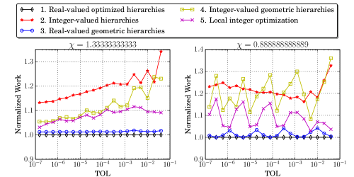
Figure 1: Ex.1: Work, according to (6), of different hierarchies normalized by the work estimate of the “real-valued” optimized hierarchy. Taking the ceiling of $h_{\ell}^{-1}$ and $M_{\ell}$ seems to produce near-optimal hierarchies. To generate these hierarchies we used the parameters of Ex.1 in Table 1 (See Remark 7).

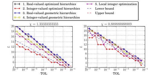
Figure 2: Ex.1: Optimal $L$ of different hierarchies. Here the bounds are from (20). To generate these hierarchies we used the parameters of Ex.1 in Table 1 (See Remark 7).

Remark 8 (When optimal hierarchies become geometric)

Recall that for $\chi\neq 1$, given $L$, $h_{0}$, and $h_{L}$ the optimal intermediate mesh sizes satisfy (52) which corresponds to the ratios

$$\frac{h_{\ell}}{h_{\ell+1}} =\left(\frac{h_{0}}{h_{L}}\right)^{\chi^{\ell}\frac{1-\chi}{1-\chi^{L}}}\chi^{\frac{2}{d\gamma}\left(\frac{L\chi^{\ell}}{1-\chi^{L}}-\frac{1}{1-\chi}\right)}$$ (33)

between successive levels. Keep the optimal choices of $h_{0}(\theta,L)$ and $h_{L}(\theta,L)$ in (2.19a), let ${\beta}$ satisfy (29) and pick $\theta$ to solve the equation

$$h_{L}(\theta,L) =h_{0}(\theta,L){\beta}^{-L}$$ (34)

given $L$. This means choosing the error splitting parameter

$$\theta=1-Q_{W}\mathrm{TOL}^{-1}{\beta}^{-q_{1}(L+1)}\left(\frac{V_{0}}{Q_{S}}\right)^{\frac{\eta}{x}}$$

for any $L\in\mathbb{N}$ sufficiently large to make the bias smaller than the total error tolerance, that is $\theta>0$. Now, by (34) the ratios (33) reduces to $h_{\ell}/h_{\ell+1}=\beta$. In other words, given $\mathrm{TOL}$, to any sufficiently large $L$ there corresponds at least one (suboptimal) $\theta$ such that the corresponding optimized hierarchy is geometric.

3 Numerical results

In this section, we first introduce the two test problems: a geometric Brownian motion SDE for which $\chi>1$ and a random PDE for which $\chi<1$ or $\chi>1$, depending on the linear solver used to solve the corresponding linear system. We then describe several implementation details and finally conclude by presenting the actual numerical results. We do not show results for the case $\chi=1$ since we proved that geometric hierarchies are optimal in this case and similar results can be found in the standard work of Giles giles08 .

3.1 Overview of examples

We consider two numerical examples for which we can compute a reference solution.

3.1.1 Ex.1

This problem is based on Example 1 in Section 2.1 with some particular choices that satisfy the assumptions therein. First, we choose ${\mathcal{D}=(0,1)^{3}}$ and assume that the forcing is

$$f(\mathbf{x})=f_{0}+\widehat{f}\sum_{i=0}^{K}\sum_{j=0}^{K}\sum_{k=0}^{K}\Phi_{ijk}(\mathbf{x})Z_{ijk},$$

where

$$\Phi_{ijk}(\mathbf{x})=\sqrt{\lambda_{i}\lambda_{j}\lambda_{k}}\phi_{i}(x_{1})\phi_{j}(x_{2})\phi_{k}(x_{3}),$$

and

$$\phi_{i}(x) =\begin{cases}\cos\left(\frac{5\Lambda i}{2}\pi x\right),&i\text{ is even},\\ \sin\left(\frac{5\Lambda(i+1)}{2}\pi x\right),&i\text{ is odd},\end{cases}$$

$$\lambda_{i} =\left(2\pi\right)^{\frac{7}{6}}\Lambda^{\frac{11}{6}}\begin{cases}\frac{1}{2},&i=0,\\ \exp\left(-2\left(\pi\frac{i}{2}\Lambda\right)^{2}\right),&i\text{ is even},\\ \exp\left(-2\left(\pi\frac{i+1}{2}\Lambda\right)^{2}\right),&i\text{ is odd},\end{cases}$$

for given parameters $\Lambda$, positive, and $K$, positive integer, and $\mathbf{Z}=\{Z_{ijk}\}$, a set of $(K+1)^{3}$ i.i.d. standard normal random variables. Moreover, we choose the diffusion coefficient to be a function of two random variables as follows:

$$a(\mathbf{x}) =a_{0}+\exp\Big{(}4Y_{1}\Phi_{121}(\mathbf{x})+40Y_{2}\Phi_{877}(\mathbf{x})\Big{)}.$$ (35)

Here, $\mathbf{Y}=\{Y_{1},Y_{2}\}$ is a set of i.i.d. standard normal random variables, also independent of $\mathbf{Z}$. Finally, we choose the quantity of interest, $g$, as a localized average around a point $\mathbf{x}_{0}$,

$$g=\left(2\pi\sigma^{2}\right)^{\frac{-3}{2}}\int_{\mathcal{D}}\exp\left(-\frac{\|\mathbf{x}-\mathbf{x}_{0}\|^{2}_{2}}{2\sigma^{2}}\right)u(\mathbf{x})d\mathbf{x},$$

and select the parameters $a_{0}=0.01,f_{0}=50,\widehat{f}=10,\Lambda=\frac{0.2}{\sqrt{2}},K=10,\sigma^{2}=0.02622863$ and ${\mathbf{x}_{0}=\left[0.5026695,0.26042876,0.62141498\right]}$. Since the diffusion coefficient, $a$, is independent of the forcing, $f$, a reference solution can be calculated to sufficient accuracy by scaling and taking expectation of the weak form with respect to $\mathbf{Z}$ to obtain a formula with constant forcing for the conditional expectation with respect to $\mathbf{Y}$. We then use stochastic collocation, bnt2010 , with a sufficiently accurate quadrature to produce the reference value, ${\mathrm{E}\mspace{-2.0mu}\left[g\right]}$. Using this method, the reference value $1.6026$ is computed with an error estimate of $10^{-4}$.

3.1.2 Ex.2

The second example is a one-dimensional geometric Brownian motion based on Example 2 where we make the following choices:

$$T =1,$$

$$a(t,u) =0.05u,$$

$$b(t,u) =0.2u,$$

$$g(u) =10\max(u(1)-1,0).$$

The exact solution can be computed using a change of variables and Itô’s formula. For the selected parameters, the solution is $1.04505835721856$.

3.2 Implementation and runs

To test the different hierarchies presented in this work we extend the CMLMC algorithm haji_CMLMC to optimal hierarchies and implement it in the C programming language. The CMLMC algorithm solves problems with tolerances larger than the requested $\mathrm{TOL}$ to cheaply get increasingly accurate estimates of the constants $Q_{W}$ and $Q_{S}$ and the variances $V_{\ell}$ for all $\ell=0,1\ldots L$. This is achieved in a Bayesian setting to incorporate the generated samples with the models (11).

We stress that with these numerical results we aim to illustrate what happens when the hierarchies of Section 2 are used in a practically viable algorithm which approximates several relevant parameters during the computations. This means that we do not directly observe the optimal hierarchies as derived in the continuous optimization.

Unless $\theta$ is specified explicitly, our CMLMC algorithm uses a computational splitting parameter, $\theta$, calculated based on the expected bias as

$$\theta=1-\frac{Q_{W}h_{L}^{q_{1}}}{\mathrm{TOL}},$$ (36)

to relax the statistical error constraint. If $h_{L}$ satisfies (15a) or (19a), this is the same as the optimal splitting parameter defined by (15c) or (19c), respectively.

For implementing the solver for the PDEs in test problem Ex.1, we use PetIGA Collier2013 . While the primary intent of this framework is to provide high-performance B-spline-based finite element discretizations, it is also useful in applications where the domain is topologically square and subject to uniform refinements. As its name suggests, PetIGA is designed to tightly couple to PETSc petsc-efficient . The framework can be thought of as an extension of the PETSc library, which provides methods for assembling matrices and vectors that result from integral equations. We use uniform meshes with a standard trilinear basis to discretize the weak form of the model problem, integrating it with eight quadrature points. We also generate results for two linear solvers for which PETSc provides an interface. The first solver is an Iterative GMRES solver that solves a linear system in almost linear time with respect to the number of degrees of freedom for the mesh sizes of interest; in other words, in this case $\gamma=1$ and $\chi>1$. The second solver is the Direct solver MUMPS Amestoy2001 . For the mesh sizes of interest, the running time of MUMPS varies from quadratic to linear in the total number of degrees of freedom. The best fit turns out to be $\gamma=1.5$ in this case, which gives $\chi<1$. From Corollary 2 (or Corollary 3), the complexity for all the examples is expected to be ${{\mathcal{O}\left(\mathrm{TOL}^{-s}\right)}}$, where $s$ depends on $q_{1},q_{2},$ and $d\gamma$. These and other problem parameters are summarized in Table 1 for the different examples. Also included in this table is the optimal level separation constant ${\beta}$, which we used when computing with geometric hierarchies. Obviously, as mentioned in Remark 5, the “real-valued” hierarchies we derived cannot always be used in practice and we follow the strategies outlined in that remark to produce “integer-valued” hierarchies that can be used.

	Ex.1	Ex.1	Ex.2
$d$	3		1
$q_{1}$	2		1
$q_{2}$	4		2
Estimated $V_{0}$	0.0565		1.7805
Estimated $Q_{W}$	1.3653		0.0307
Estimated $Q_{S}$	0.1519		0.2630
Solver	GMRES	MUMPS	Milstein
$\gamma$	1	1.5	1
$\chi$	4/3	8/9	2
$\eta$	2/3	4/9	1
$s$	2	2.25	2
Optimal ${\beta}$	1.7778	1.6018	4
Work to seconds constant	$10^{-4}$	$3\times 10^{-6}$	$9\times 10^{-8}$

Table 1: Summary of problem parameters.

We run each setting $100$ times and show in plots in the next section the medians with vertical bars spanning from the $5\%$ percentile to the $95\%$ percentile. Finally, all results were generated on the same machine with $52$ gigabytes of memory to ensure that no overhead is introduced due to hard disk access during swapping that could occur when solving the three-dimensional PDEs with a fine mesh. We use the parameters listed in Table 2 for the CMLMC algorithm haji_CMLMC .

Parameter	Purpose	Value for Ex.1	Value for Ex.2
$\kappa_{0}$ and $\kappa_{1}$	Confidence parameter for the weak and strong error models	$0.1$ for both	$0.1$ for both
$\mathrm{TOL}_{\max}$	The maximum tolerance with which to start the algorithm.	0.5	0.1
$r_{1}$ and $r_{2}$	Controls computational burden to calibrate the problem parameters.	$2$ and $1.1$, respectively	$2$ and $1.1$, respectively
Initial hierarchy	The initial hierarchy to start the CMLMC algorithm.	$L=2$ and $h_{\ell}^{-1}=\{4,6,8\}$ and $M_{\ell}=10$ for all $\ell$.	$L=2$ and $h_{\ell}^{-1}=\{1,2,4\}$ and $M_{\ell}=10$ for all $\ell$.
$L_{\text{inc}}$	Maximum number of values to consider when optimizing for L.	2	2
$\mathfrak{L}$	Maximum number of levels used to compute estimates of $Q_{W}$ and $Q_{S}$.	3	5
$C_{\alpha}$	Parameter related to the confidence in the statistical constraint	2	2

Table 2: Summary of parameter values used in the CMLMC algorithm in our numerical tests. This table is reproduced from haji_CMLMC where more information is available.

3.3 Results

We start by presenting the results of Ex.1. We show in Figure 3 the total running time of the CMLMC algorithm and its last iteration when using optimal hierarchies, after taking the ceiling of the optimal number of elements $h_{\ell}^{-1}$ in (19a) and the optimal number of samples $M_{\ell}$ in (13). Using the parameters in 1, we also show in this figure the expected running time when using the optimal, unconstrained hierarchy defined by (19) and the expected asymptotic work according to Corollary (2). This figure shows good agreement between the expected theoretical results and the actual final running time. Figure 4 shows that the true error that was computed using the reference solution when using optimal hierarchies is less than the required tolerance with the required confidence of $95\%$, in accordance with the chosen value of $C_{\alpha}=2$ and (haji_CMLMC, , Lemma A.2). Figure 5 compares the computational complexity of optimal hierarchies to geometric hierarchies for different values of $\theta$. This figure shows numerical confirmation that optimal hierarchies do not give significant improvement over geometric hierarchies, especially for optimal values of $\theta$. In other words, the improvement of the running time is mainly due the better choice of $\theta$ as discussed in haji_CMLMC . Figure 7 shows the optimal splitting, $\theta$, as defined by (19c). Compare this figure to Figure 6, which shows the used number of levels, $L$, for different tolerances, and notice the dependence of $\theta$ on the number of levels, $L$. On the other hand, Figure 8 shows the computational splitting used in the CMLMC algorithm. Notice that $\theta$ follows a similar pattern in both Figure 7 and Figure 8. The continuous change in the latter is due to differences in the estimation of $Q_{W}$ for different runs of the algorithm. For comparison, Figure 9 shows that the computational splitting parameter produced when using geometric hierarchies is different from the computational splitting parameter produced when using optimal hierarchies. However, as $\mathrm{TOL}\to 0$, they both seem to be not too far from the limit in (25). Finally, even though (haji_CMLMC, , Lemma A.2) assumes a geometric sequence, Figure 10 shows that the lemma still holds for non-geometric hierarchies; i.e., that the cumulative density function (CDF) of the true error when suitably normalized is well approximated by a standard normal CDF.

Next, we focus on Ex.2 where $\chi=2$ using the Milstein scheme. Since we showed previously that geometric hierarchies are near-optimal, we only present the results when using geometric hierarchies in this case. The optimal geometric constant, ${\beta}$, is $4$ in this case according to (29). Figure 11 shows that the actual running time of the CMLMC algorithm has the expected rate $\mathrm{TOL}^{-2}$, again as predicted in Corollary 3, or indeed for these nested geometric hierarchies already in giles08_m . Figure 12 shows that the true errors for different tolerances are less than the required tolerance with the required confidence of $95\%$.

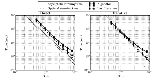
Figure 3: Ex.1: The running time of the CMLMC algorithm and its last iteration when using optimal hierarchies. Using the parameters in 1, we also show in this figure the expected running time when using the optimal, unconstrained hierarchy defined by (19) and the expected asymptotic work according to Corollary (2).

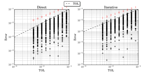
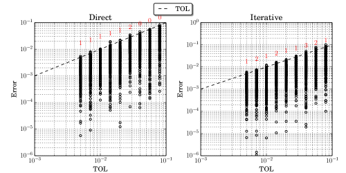
Figure 4: Ex.1: The true errors calculated using optimal hierarchies in the top plot, and using geometric hierarchies in the bottom one. Each point shows the true error of an independent run of MLMC. The numbers on top of the $\mathrm{TOL}$ line are the percentage of algorithm runs that produced a larger error than the required tolerance. Notice that the choice $C_{\alpha}=2$ gives a confidence of a $95\%$ in the error bound, as predicted in (haji_CMLMC, , Lemma A.2).

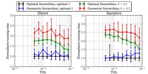
Figure 5: Ex.1: Actual running time of the CMLMC algorithm when using optimal and geometric hierarchies with different tolerance splitting, normalized by the average running time of the algorithm when using optimal hierarchies. Compare this figure to Figure 1, where the latter is based on the theoretical results. Observe that most of the gain in computational complexity is due to the choice (36) of $\theta$ and that using optimal hierarchies does not significantly improve the running time over geometric hierarchies.

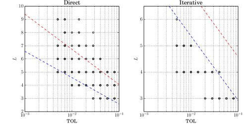
Figure 6: Ex.1: The used number of levels, $L$, for different tolerances in the last iteration of the CMLMC algorithm when using optimal hierarchies and ceiling $h_{\ell}^{-1}$ and $M_{\ell}$. Here, different circles correspond to independent runs of CMLMC. Compare this figure to the Figure 2, where the latter is based on the theoretical results. The bounds are taken from (20). The $L$ values used by the CMLMC algorithm fall outside the predicted bounds because the bounds are valid for the real-valued optimal hierarchies only. On the other hand, CMLMC is constrained to the discrete sets of feasible hierarchies and further limits the increments of $L$ across iterations.

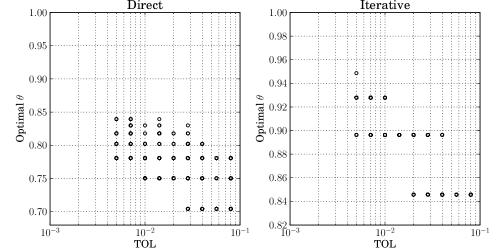
Figure 7: Ex.1: The error splitting parameter, $\theta$, as defined by (19c). Recall that $\theta$ depends on $L$ and notice the correspondence to $L$ values in Figure 6

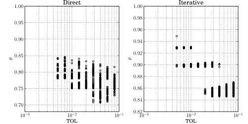
Figure 8: Ex.1: The computational splitting parameter, $\theta$, as defined in (36) for the CMLMC algorithm for optimal hierarchies. Though these $\theta$ values correspond to the value in Figure 7, the differences are due to enforcing constraints on $h_{L}$.

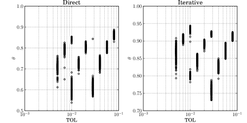
Figure 9: Ex.1: The computational splitting parameter, $\theta$, in the CMLMC algorithm for optimal geometric hierarchies.

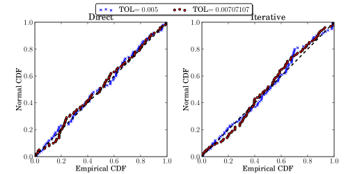
Figure 10: Ex.1: A QQ-plot indicating that, even when using non-geometric hierarchies, the distribution of the normalized statistical error is well approximated by the standard normal density. The work (haji_CMLMC, , Lemma A.2) proved such results for geometric hierarchies.

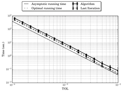
Figure 11: Ex.2: The running time of the CMLMC algorithm. The reference dashed line is ${\mathcal{O}\left(\mathrm{TOL}^{-2}\right)}$ as predicted in (tsgu13, , Theorem 2.3).

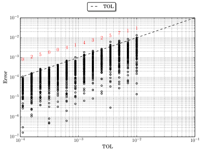
Figure 12: Ex.2: The true errors calculated using geometric hierarchies with ${\beta}=4$. The numbers on top of the $\mathrm{TOL}$ line are the percentage of algorithm runs that produced a larger error than the required tolerance. Remember that $C_{\alpha}=2$ gives a confidence of a $95\%$ in the error bound, as predicted in (haji_CMLMC, , Lemma A.2).

4 Conclusions

MLMC sampling methods are becoming increasingly popular due to their robustness and simplicity. In this work, in Theorems 2.1 and 2.2 and Corollary 3, we have developed optimal non-geometric and geometric hierarchies for MLMC by assuming certain asymptotic models on the weak and strong convergence and the average computational cost per sample. While it is important to optimize the geometric level separation parameter, $\beta$, and the tolerance splitting parameter, $\theta$, to obtain significant computational savings, we have shown, in Remark 6, that with these optimized parameters, geometric hierarchies are nearly optimal and that, asymptotically, their computational complexity is the same as the non-geometric optimal hierarchies. Moreover, we have analyzed the asymptotic behavior of the optimal tolerance splitting parameter, $\theta$, between the bias and the statistical error contribution. We have also discussed how enforcing constraints on parameters of MLMC hierarchies affects the optimality of these hierarchies. These constraints include an upper and lower bound on the mesh size or enforcing that the number of samples and the number of discretization elements are integers. Our numerical results show remarkable agreement between our theory of optimal hierarchies and their asymptotic behavior and the performance of the CMLMC algorithm.

In future work, it is possible to improve the efficiency of the MLMC method by including certain non-asymptotic terms in the models for the weak and strong convergence or the computational complexity. Moreover, since the asymptotic dependence of the computational complexity on the different problem constants is clearly shown in Corollaries 1 and 2, one can devise methods to combine with MLMC to reduce the total computational complexity by affecting these constants, for example by reducing the variance, $V_{0}$, for the case where $\chi>1$.

Appendix A Derivations and proofs

A.1 Optimal hierarchies given $h_{0}$, $\theta$, and $L$

Here we solve Problem 1 of Section 2.2 for the optimal hierarchy for any fixed value of $L$. We initially treat the parameter $\theta$ as given, postponing its optimization until later, and proceed in two steps to find the optimal $\{M_{\ell}\}_{\ell=0}^{L}$ and $\{h_{\ell}\}_{\ell=0}^{L}$. Assuming general work estimates $\{W_{\ell}\}_{\ell=0}^{L}$ in (4) and general variance estimates of $\{V_{\ell}\}_{\ell=0}^{L}$, we assume equality in (9b) and introduce the Lagrange multiplier $\lambda$ to obtain the Lagrangian

$$\mathcal{L}\left(\{M_{\ell}\}_{\ell=0}^{L},\lambda\right) =\sum_{\ell=0}^{L}M_{\ell}W_{\ell}+\lambda\left\{\sum_{\ell=0}^{L}\frac{V_{\ell}}{M_{\ell}}-\left(\theta\frac{\mathrm{TOL}}{C_{\alpha}}\right)^{2}\right\}.$$

The requirement that the variation of the Lagrangian with respect to $M_{\ell}$ is zero, gives $M_{\ell}=\sqrt{\lambda\frac{V_{\ell}}{W_{\ell}}}.$ Solving for $\lambda$ in the variance constraint (9b) and substituting back leads to (13). Substituting this optimal $M_{\ell}$ in the total work (4) yields

$$W(\mathbf{H}) =\left(\frac{C_{\alpha}}{\theta\mathrm{TOL}}\right)^{2}\left(\sum_{\ell=0}^{L}\sqrt{W_{\ell}V_{\ell}}\right)^{2}.$$ (37)

We proceed to find the optimal $\{h_{\ell}\}_{\ell=0}^{L}$ under the particular models (12). The total work (37) is minimized when

$$\sum_{\ell=0}^{L}\sqrt{W_{\ell}V_{\ell}} =\sqrt{\frac{{V_{0}}}{h_{0}^{d\gamma}}}+\sqrt{Q_{S}}\sum_{\ell=1}^{L}\sqrt{\frac{h_{\ell-1}^{q_{2}}}{h_{\ell}^{d\gamma}}},$$ (38)

is minimized. Here the finest mesh, $h_{L}$, is given by the bias constraint (12b) as

$$h_{L} =\left(\frac{(1-\theta)\,\mathrm{TOL}}{Q_{W}}\right)^{\frac{1}{q_{1}}},$$ (39)

independently of the multilevel construction. Now, treat the coarsest mesh, $h_{0}$, as given and find the optimal $h_{1},\ldots,h_{L-1}$ that minimize

$$\frac{1}{\sqrt{Q_{S}}}\sum_{\ell=1}^{L}\sqrt{W_{\ell}V_{\ell}} =\sum_{\ell=1}^{L}\sqrt{\frac{h_{\ell-1}^{q_{2}}}{h_{\ell}^{d\gamma}}}.$$ (40)

The requirement that the derivative of this sum with respect to $h_{\ell}$ equals zero, for $\ell=1,\ldots,L-1$, leads to the optimality condition

$$q_{2}h_{\ell}^{\left(\frac{q_{2}+d\gamma}{2}\right)} =d\gamma h_{\ell-1}^{\left(\frac{q_{2}}{2}\right)}h_{\ell+1}^{\left(\frac{d\gamma}{2}\right)},$$

which after taking the logarithm and using $\chi$ defined in (14), leads to

$$-\log{\left(h_{\ell+1}\right)}+\left(1+\chi\right)\log{\left(h_{\ell}\right)}-\chi\log{\left(h_{\ell-1}\right)} =-\frac{2}{d\gamma}\log{\left(\chi\right)}.$$ (41)

This is a second order linear difference whose solution depends on $\chi$.

A.1.1 For $\chi=1$

This section provides proofs of Theorem 2.1, Lemma 1, and Corollary 1. The solution of the difference equation (41) for the case $\chi=1$ is the geometric sequence

$$h_{\ell} =h_{0}{\beta}^{-\ell}, {\beta}=\left(\frac{h_{0}}{h_{L}}\right)^{1/L}$$ with . (42)

In other words, all $h_{\ell}$ are defined in terms of $h_{0}$ and $h_{L}$, where the latter is determined by $\theta$ through (39) and we solve for the former by setting the derivative of (38) with respect to $h_{0}$ equal to zero. This optimality condition becomes (for $q_{2}=d\gamma$)

$$h_{1}=\left(\frac{Q_{S}}{V_{0}}\right)^{\frac{1}{q_{2}}}h_{0}^{2}.$$

Combining this expression with (42) for $\ell=1$ and solving for $h_{0}$ yields

$$h_{0}=h_{L}^{\frac{1}{L+1}}\left(\frac{V_{0}}{Q_{S}}\right)^{\frac{L}{q_{2}(L+1)}}.$$ (43)

Substituting this expression and (39) in the expression for ${\beta}$ in (42) we obtain (15c). Moreover, substituting (15c) and (42) and (10) and (5) in (13) yields (15b). Next, we substitute (15b) and (15a) in (6) to obtain the optimal work for $q_{2}=d\gamma$

$$W=\left(\frac{C_{\alpha}}{\theta\mathrm{TOL}}\right)^{2}\left(\sqrt{V_{0}}h_{0}^{\frac{-q_{2}}{2}}+\sqrt{Q_{S}}{\beta}^{\frac{q_{2}}{2}}L\right)^{2}.$$ (44)

Using (42) and (43), we obtain

$$W=\left(\frac{C_{\alpha}}{\theta\mathrm{TOL}}\right)^{2}h_{L}^{\frac{-q_{2}}{L+1}}V_{0}^{\frac{1}{L+1}}Q_{S}^{\frac{L}{L+1}}\left(1+L\right)^{2}.$$ (45)

Substituting for $h_{L}$ from (39)

$$W=\left(\frac{C_{\alpha}}{\theta\mathrm{TOL}}\right)^{2}\left(\frac{Q_{W}}{(1-\theta)\,\mathrm{TOL}}\right)^{\frac{1}{\eta(L+1)}}V_{0}^{\frac{1}{L+1}}Q_{S}^{\frac{L}{L+1}}\left(1+L\right)^{2}.$$ (46)

Optimizing for $\theta$ yields (15d). Substituting back gives the work as a function of $L$

$$W(L)=C_{\alpha}^{2}\mathrm{TOL}^{-2(1+\mathfrak{e}(L))}Q_{W}^{2\mathfrak{e}(L)}V_{0}^{2\eta\mathfrak{e}(L)}Q_{S}^{-2\eta\mathfrak{e}(L)}Q_{S}\left(\frac{1}{2\eta}\right)^{2}\left(1+\frac{1}{\mathfrak{e}(L)}\right)^{2(1+\mathfrak{e}(L))},$$ (47)

where $\mathfrak{e}(L)=\frac{1}{2\eta(L+1)}$. Treating $L$ as a continuous variable and differentiating with respect to $L$ yields

$$W^{\prime}(L)=2W(L)\mathfrak{e}^{\prime}(L)\left(C-y+\log(1+y)\right),$$ (48)

where ${y=2\eta(L+1)}>0$ and ${C=\log\left(\mathrm{TOL}^{-1}Q_{W}V_{0}^{\eta}Q_{S}^{-\eta}\right)}$. Setting (48) to zero gives the equation

$$y-\log(1+y)=C.$$ (49)

It follows that $\lim_{C\to\infty}\frac{y}{C}=1$ which leads to (17) for the value of $L$ and (18) for the work. Since $y>0$, equation (49) implies

$$1<yC^{-1}$$ (50)

for any $C>0$. Furthermore, for any $y>0$, it holds

$$\left(\frac{\exp(1)-1}{\exp(1)}\right)(1+y)-C\leq 1+y-\log(1+y)-C,$$

which together with (49) gives

$$yC^{-1}\leq\frac{\exp(1)}{\exp(1)-1}+\frac{1}{(\exp(1)-1)C},$$ (51)

for any $C>0$. Inequalities (50) and (51) are (16).

A.1.2 For $\chi\neq 1$

This section provides proofs of Theorem 2.2, Lemma 2, and Corollary 2. The solution of the difference equation (41) for the case $\chi\neq 1$ is

$$h_{\ell} =h_{0}^{\left(\frac{\chi^{\ell}-\chi^{L}}{1-\chi^{L}}\right)}h_{L}^{\left(\frac{1-\chi^{\ell}}{1-\chi^{L}}\right)}\chi^{-\frac{2}{d\gamma}\left(\frac{L(1-\chi^{\ell})-\ell(1-\chi^{L})}{(1-\chi)(1-\chi^{L})}\right)}.$$ (52)

We now distinguish between two different cases for $h_{0}$: either we are free to choose the optimal $h_{0}\in\mathbb{R}_{+}$, or we have an upper bound on the coarsest mesh $h_{0}$. The first, idealized, situation will allow us to obtain explicit expressions for the optimal splitting parameter $\theta$ and the asymptotic work, and we start by considering this case. We return to the other case at the end of this section.

Unconstrained optimization of $h_{0}$

We take $h_{1},\ldots,h_{L}$ given by (52) and (39) and set the derivative of (38) with respect to $h_{0}$ equal to zero. This optimality condition becomes (after some straightforward simplifications)

$$-\frac{d\gamma}{2}\frac{\sqrt{{V_{0}}}}{h_{0}^{1+d\gamma/2}}+\frac{q_{2}}{2}\sqrt{Q_{S}}\frac{h_{0}^{q_{2}/2-1}}{h_{1}^{d\gamma/2}} =0,$$

which, since all parameters are positive, is equivalent to

$$h_{1} =\left(\frac{\chi^{2}Q_{S}}{{V_{0}}}\right)^{\frac{1}{d\gamma}}h_{0}^{1+\chi}.$$

Combining this expression for $h_{1}$ with the one in (52) and solving for $h_{0}$ gives

$$h_{0} =h_{L}^{\frac{1-\chi}{1-\chi^{L+1}}}\left(\frac{{V_{0}}}{Q_{S}}\right)^{\frac{1}{d\gamma}\frac{1-\chi^{L}}{1-\chi^{L+1}}}\chi^{-\frac{2}{d\gamma}\frac{1}{1-\chi}\left(L\frac{1-\chi}{1-\chi^{L+1}}-\chi\frac{1-\chi^{L}}{1-\chi^{L+1}}\right)},$$

which after substituting back into (52) and using (39) yields (19a). Finally substituting these optimal mesh sizes into (13) yields (19b).

Optimal splitting parameter $\theta$

Now the sequences $\{h_{\ell}\}_{\ell=0}^{L}$ and $\{M_{\ell}\}_{\ell=0}^{L}$ are determined in terms of the still not optimized $L$ and $\theta$ as well as measurable model parameters. The work per level in (6) becomes

$$\frac{M_{\ell}}{h_{\ell}^{d\gamma}} =\left(\frac{C_{\alpha}}{\theta\mathrm{TOL}}\right)^{2}\left(\frac{Q_{W}}{(1-\theta)\,\mathrm{TOL}}\right)^{\frac{1}{\eta}\frac{1-\chi}{1-\chi^{L+1}}}V_{0}\left(\frac{Q_{S}}{V_{0}}\right)^{\left\{\frac{1-\chi^{L}}{1-\chi^{L+1}}\right\}}$$

$$\quad\cdot\frac{1-\chi^{L+1}}{1-\chi}\chi^{\left\{-\frac{2\chi}{1-\chi}\frac{1-\chi^{L}}{1-\chi^{L+1}}+L\frac{1+\chi^{L+1}}{1-\chi^{L+1}}\right\}}\chi^{-\ell}.$$

Since the only $\ell$-dependent factor in the right hand side is the last one, $\chi^{-\ell}$, and using $\sum_{\ell=0}^{L}\chi^{-\ell}=\chi^{-L}(1-\chi^{L+1})/(1-\chi)$, the total work in (6) becomes

$$W{(L,\theta,\mathrm{TOL})} =w_{1}\left(L,\mathrm{TOL}\right)\,w_{2}(L)\,f\left(L,\theta\right)\left(\frac{1-\chi^{L+1}}{1-\chi}\right)^{2},$$ (53)

with

$$w_{1}\left(L,\mathrm{TOL}\right) =\mathrm{TOL}^{-\left(2+\frac{1}{\eta}\frac{1-\chi}{1-\chi^{L+1}}\right)},$$ (54a)

$$w_{2}(L) =C_{\alpha}^{2}\,V_{0}\left(\frac{Q_{S}}{V_{0}}\right)^{\left\{\frac{1-\chi^{L}}{1-\chi^{L+1}}\right\}}Q_{W}^{\left\{\frac{1}{\eta}\frac{1-\chi}{1-\chi^{L+1}}\right\}}$$ (54b)

$$\quad\cdot\chi^{\left\{-\frac{2\chi}{1-\chi}\frac{1-\chi^{L}}{1-\chi^{L+1}}+2L\frac{\chi^{L+1}}{1-\chi^{L+1}}\right\}},$$

$$f\left(L,\theta\right) =\frac{1}{\theta^{2}\left(1-\theta\right)^{\frac{1}{\eta}\frac{1-\chi}{1-\chi^{L+1}}}}.$$ (54c)

Thus given the value of $L$ the dependence on the splitting parameter $\theta$ is straightforward, and the minimal work for a given $L$ is obtained with the minimizer of (54c), namely (19c). With this optimal splitting parameter $\theta$ in (53) the total work as a function of the yet to be determined parameter $L$ and the tolerance is

$$W{\left(L,\mathrm{TOL}\right)} =w_{1}(L,\mathrm{TOL})\,w_{2}(L)\,w_{3}(L),$$ (55)

with

$$w_{3}(L) =\left(\frac{1}{2\eta}\right)^{2}\left(1+2\eta\frac{1-\chi^{L+1}}{1-\chi}\right)^{2\left(1+\frac{1}{2\eta}\frac{1-\chi}{1-\chi^{L+1}}\right)}.$$ (56)

Optimal number of levels

The optimal integer $L$ seems impossible to find analytically. In practical computations we instead perform an extensive search over a small range of integer values. In the analysis below we treat $L$ as a real parameter to obtain the bounds (20) that delimit the range of integer values that must be tested, and allow a complexity analysis as $\mathrm{TOL}\to 0$ without an exactly determined $L$.

Treating $L$ as a real parameter, we differentiate the work (55) with respect to $L$ to obtain

$$\frac{\partial W}{\partial L} =\frac{\partial w_{1}}{\partial L}\,w_{2}\,w_{3}+w_{1}\,\frac{\partial w_{2}}{\partial L}\,w_{3}+w_{1}\,w_{2}\,\frac{\partial w_{3}}{\partial L},$$

where, introducing the shorthand

$$\xi(L) =2\eta\frac{1-\chi^{L+1}}{1-\chi} \text{for }L\in[0,\infty),$$ (57)

and using the constants $c_{1}$ and $c_{2}$ in (21) we write

$$\frac{\partial w_{1}}{\partial L} =w_{1}(L,\mathrm{TOL})\,\frac{\log{(\chi)}\,\chi^{L+1}}{1-\chi^{L+1}}\frac{2}{\xi(L)}\log{\left(\mathrm{TOL}^{-1}\right)},$$ (58a)

$$\frac{\partial w_{2}}{\partial L} =w_{2}(L)\,\frac{\log{(\chi)}\,\chi^{L+1}}{1-\chi^{L+1}}\frac{2}{\xi(L)}\left(c_{1}+-c_{2}(L+1)+\xi(L)\right),$$ (58b)

$$\frac{\partial w_{3}}{\partial L} =w_{3}(L)\,\frac{\log{(\chi)}\,\chi^{L+1}}{1-\chi^{L+1}}\frac{2}{\xi(L)}\big{(}\log{\left(1+\xi(L)\right)}-\xi(L)\big{)},$$ (58c)

so that

$$\frac{\partial W}{\partial L}(L,\mathrm{TOL}) =u(L,\mathrm{TOL})v(L,\mathrm{TOL}),$$ (59)

with

$$u(L,\mathrm{TOL}) =W{(L,\mathrm{TOL})}\,\frac{\log{(\chi)}\,\chi^{L+1}}{1-\chi^{L+1}}\frac{2}{\xi(L)},$$

$$v(L,\mathrm{TOL}) =\log{\left(\mathrm{TOL}^{-1}\right)}+c_{1}+-c_{2}(L+1)+\log{\left(1+\xi(L)\right)}.$$

Clearly $u(L,\mathrm{TOL})<0$ for all $\chi\in\mathbb{R}_{+}\setminus\{1\}$ so the sign of $\partial W/\partial L$ is the opposite of the sign of $v(L,\mathrm{TOL})$. For a fixed $\chi\in\mathbb{R}_{+}\setminus\{1\}$ we have

$$v(L,\mathrm{TOL})>0 \Leftrightarrow L+1<\frac{1}{c_{2}}\left(\log{\left(\mathrm{TOL}^{-1}\right)}+c_{1}+\log{\left(1+\xi(L)\right)}\right),$$

and, since $\xi(L)\geq\xi(0)=2\eta$,

$$L+1<\frac{1}{c_{2}}\left(\log{\left(\mathrm{TOL}^{-1}\right)}+c_{1}+\log{\left(1+2\eta\right)}\right) \Rightarrow v(L,\mathrm{TOL})>0\Leftrightarrow\frac{\partial W}{\partial L}<0.$$ (60)

For the opposite inequality,

$$v(L,\mathrm{TOL})<0 \Leftrightarrow L+1>\frac{1}{c_{2}}\left(\log{\left(\mathrm{TOL}^{-1}\right)}+c_{1}+\log{\left(1+\xi(L)\right)}\right),$$

we distinguish between the cases $0<\chi<1$ and $1<\chi$. When $0<\chi<1$ we have the upper bound $\xi(L)<\frac{2\eta}{1-\chi}$ and consequently

$$L+1>\frac{1}{c_{2}}\left(\log{\left(\mathrm{TOL}^{-1}\right)}+c_{1}+\log{\left(1+\frac{2\eta}{1-\chi}\right)}\right) \Rightarrow\frac{\partial W}{\partial L}>0, \chi\in(0,1).$$ (61)

In contrast $\xi(L)$ is unbounded when $1<\chi$ but, since the definitions of $\chi$ and $\eta$ and the relation between strong and weak convergence orders implies that $2\eta\geq\chi$, we have

$$\log{\left(1+\xi(L)\right)} <\log{\left(\frac{2\eta}{\chi-1}\right)}+(L+1)\log{\chi},$$

and

$$c_{2} \geq\frac{\chi}{\chi-1}\log{\chi},$$

which gives the bound

$$\frac{1}{c_{2}}\log{\left(1+\xi(L)\right)} <\frac{\chi-1}{\chi}(L+1)+\frac{1}{c_{2}}\log{\left(\frac{2\eta}{\chi-1}\right)}.$$

Hence

$$L+1-\frac{1}{c_{2}}\log{\left(1+\xi(L)\right)} >\frac{L+1}{\chi}-\frac{1}{c_{2}}\log{\left(\frac{2\eta}{\chi-1}\right)},$$

and it follows that

$$L+1>\frac{\chi}{c_{2}}\left(\log{\left(\mathrm{TOL}^{-1}\right)}+c_{1}+\log{\left(\frac{2\eta}{\chi-1}\right)}\right) \Rightarrow\frac{\partial W}{\partial L}>0, \chi\in(1,\infty).$$ (62)

Combining (60) with (61) and (62), we obtain the bounds (20).

Optimal hierarchies with an upper bound on $h_{0}$

Practical computations will impose an upper limit on the mesh sizes, $h_{0}\leq h_{\mathrm{max}}$. If the mesh sizes (19a) violate such a bound, we must modify our analysis slightly. We now consider $h_{0}$ given as one of the coarsest mesh sizes that can be realized in the given discretization, and analyze the case $L\geq 1$. Using the optimal mesh sizes (52) yields

$$\sqrt{\frac{h_{\ell-1}^{q_{2}}}{h_{\ell}^{d\gamma}}} =h_{0}^{\frac{d\gamma}{2}\chi^{L}\frac{1-\chi}{1-\chi^{L}}}h_{L}^{-\frac{d\gamma}{2}\frac{1-\chi}{1-\chi^{L}}}\chi^{\left(\frac{L}{1-\chi^{L}}-\frac{\chi}{1-\chi}-\ell\right)},$$

where the only $\ell$-dependent factor in the right hand side is the last one, $\chi^{-\ell}$, so that the sum in (40) is

$$\sum_{\ell=1}^{L}\sqrt{\frac{h_{\ell-1}^{q_{2}}}{h_{\ell}^{d\gamma}}} =\left(\frac{h_{0}^{\left(\chi^{L}\right)}}{h_{L}}\right)^{\frac{d\gamma}{2}\frac{1-\chi}{1-\chi^{L}}}\chi^{\left(\frac{L\chi^{L}}{1-\chi^{L}}-\frac{\chi}{1-\chi}\right)}\frac{1-\chi^{L}}{1-\chi}.$$

In this sum only $h_{L}$ depends on $\theta$ through (39). Keeping $L$ fixed we wish to minimize the total work, which by (37)–(38) is

$$W(\mathbf{H}) =\left(\frac{C_{\alpha}}{\theta\mathrm{TOL}}\right)^{2}\left(\sqrt{\frac{{V_{0}}}{h_{0}^{d\gamma}}}+\sqrt{Q_{S}}\left(\frac{h_{0}^{\left(\chi^{L}\right)}}{h_{L}}\right)^{\frac{d\gamma}{2}\frac{1-\chi}{1-\chi^{L}}}\chi^{\left(\frac{L\chi^{L}}{1-\chi^{L}}-\frac{\chi}{1-\chi}\right)}\frac{1-\chi^{L}}{1-\chi}\right)^{2},$$

with respect to $\theta$. Letting

$$\Delta =\frac{1}{2\eta}\frac{1-\chi}{1-\chi^{L}},$$

and

$$C =\sqrt{\frac{Q_{S}}{{V_{0}}}}h_{0}^{\frac{d\gamma}{2}\frac{1-\chi^{L+1}}{1-\chi^{L}}}\chi^{\left(\frac{L\chi^{L}}{1-\chi^{L}}-\frac{\chi}{1-\chi}\right)}\frac{1-\chi^{L}}{1-\chi}\left(\frac{Q_{W}}{\mathrm{TOL}}\right)^{\Delta},$$

we obtain

$$W(\mathbf{H}) \propto\tilde{f}\left(\theta,L,h_{0}\right)=\frac{1}{\theta^{2}}\left(1+\frac{C}{\left(1-\theta\right)^{\Delta}}\right)^{2},$$

with the optimality condition

$$\frac{\partial\tilde{f}}{\partial\theta} =\frac{2}{\theta^{2}}\left(1+\frac{C}{\left(1-\theta\right)^{\Delta}}\right)\left(\frac{C\Delta}{\left(1-\theta\right)^{\Delta+1}}-\frac{1}{\theta}\left(1+\frac{C}{\left(1-\theta\right)^{\Delta}}\right)\right)=0,$$

where

$$\frac{2}{\theta^{2}}\left(1+\frac{C}{\left(1-\theta\right)^{\Delta}}\right) >0.$$

In this case when $h_{0}$ is constrained we no longer have an explicit expression for the optimal $\theta$. However, using

$$\frac{C\Delta}{\left(1-\theta\right)^{\Delta+1}}-\frac{1}{\theta}\left(1+\frac{C}{\left(1-\theta\right)^{\Delta}}\right) <\frac{C}{\left(1-\theta\right)^{\Delta}}\left(\frac{\Delta}{1-\theta}-\frac{1}{\theta}\right),$$

and that

$$\frac{\Delta}{1-\theta}-\frac{1}{\theta}=0 \Leftrightarrow\theta=\frac{1}{1+\Delta},$$

we conclude that the optimal $\theta$ satisfies

$$\frac{1}{1+\Delta} \leq\theta.$$ (63)

Similarly, from the inequality

$$\frac{C\Delta}{\left(1-\theta\right)^{\Delta+1}}-\frac{1}{\theta}\left(1+\frac{C}{\left(1-\theta\right)^{\Delta}}\right) >\frac{1}{\left(1-\theta\right)^{\Delta}}\left(\frac{C\Delta}{1-\theta}-\frac{1+C}{\theta}\right),$$

and the relation

$$\frac{C\Delta}{1-\theta}-\frac{1+C}{\theta}=0 \Leftrightarrow\theta=\frac{1+C}{1+C+\Delta},$$

we obtain an upper bound for $\theta$, namely

$$\theta \leq\frac{1+C}{1+C+C\Delta}.$$ (64)

Finally, combining (63) and (64) we have the following bounds for the optimal $\theta$:

$$\left(1+\frac{1}{2\eta}\frac{1-\chi}{1-\chi^{L}}\right)^{-1}\leq\theta\leq\left(1+\frac{1}{2\eta}\frac{1-\chi}{1-\chi^{L}}\frac{C}{1+C}\right)^{-1},$$ (65)

where the upper bound has a non-trivial dependence on $\mathrm{TOL}$ and $L$ through $C$.

A.2 Heuristic optimization of geometric hierarchies

This section motivates the results in Section 2.3 and Corollary 3 where we optimized geometric hierarchies defined by $h_{\ell}=h_{0}{\beta}^{-\ell}$ for given $h_{0}$ and ${\beta}>1$. In this case, the work and variance models are in (28) and $L$ is must satisfy the bias constraint

$$L \geq\frac{\log{(h_{0})}-\frac{1}{q_{1}}\log{\left(\frac{(1-\theta)\mathrm{TOL}}{Q_{W}}\right)}}{\log({\beta})}.$$ (66)

We distinguish between two cases:

• $\chi=1$: Or equivalently $q_{2}=d\gamma$. In this case, the total work defined in (37) simplifies to

$$W=\left(\frac{C_{\alpha}}{\theta\mathrm{TOL}}\right)^{2}\left(\sqrt{V_{0}}h_{0}^{\frac{-q_{2}}{2}}+L\sqrt{Q_{S}}\beta^{\frac{q_{2}}{2}}\right)^{2},$$ (67)

We make the simplification of treating $L$ as a real parameter and substitute the lower bound of (66) in (67) and optimize with respect to ${\beta}$ to get ${\beta}=\exp\left(\frac{2}{q_{2}}\right)$. Substituting this choice and (30), the total work satisfies

$$\frac{W}{\mathrm{TOL}^{-2}\left(\log{\mathrm{TOL}}\right)^{2}}\to\theta^{-2}C_{\alpha}^{2}Q_{S}\exp(2)\left(\frac{1}{2\eta}\right)^{2},\qquad\text{as }\mathrm{TOL}\to 0.$$

Optimizing for $\theta$ suggests that $\theta\to 1$ as $\mathrm{TOL}\to 0$ and (18) follows.

• $\chi\neq 1$: In this case, the total work defined in (37) simplifies to

$$W=\left(\frac{C_{\alpha}}{\theta\mathrm{TOL}}\right)^{2}h_{0}^{d\gamma(\chi-1)}\left(\sqrt{V_{0}}h_{0}^{\frac{-q_{2}}{2}}+\sqrt{Q_{S}}\frac{\left(1-{\beta}^{\frac{L(d\gamma-q_{2})}{2}}\right)}{{\beta}^{-\frac{d\gamma}{2}}-{\beta}^{-\frac{q_{2}}{2}}}\right)^{2},$$ (68)

for a given $L,h_{0}$ and $\theta$. Again, we make the simplification of treating $L$ as a real parameter and substitute the lower bound (66) to obtain

$${\beta}^{\frac{L(d\gamma-q_{2})}{2}}=\left(\frac{(1-\theta)\mathrm{TOL}}{Q_{W}}\right)^{\frac{\chi-1}{2\eta}}h_{0}^{\frac{d\gamma(1-\chi)}{2}},$$

for any ${\beta}$. Substituting back in (68) and optimizing with respect to ${\beta}$ to minimize the work gives (29). Substituting this optimal ${\beta}$ in (68) yields

$$W=\left(\frac{C_{\alpha}}{\theta\mathrm{TOL}}\right)^{2}h_{0}^{d\gamma(\chi-1)}\left(\sqrt{V_{0}}h_{0}^{\frac{-q_{2}}{2}}+\sqrt{Q_{S}}\frac{\chi^{\frac{\chi}{\chi-1}}}{\chi-1}\left(1-\chi^{-L}\right)\right)^{2}.$$ (69)

Asymptotically, using (30) as $\mathrm{TOL}\to 0$ yields (23) with the following constants

$$C_{1} =(1-\theta)^{\frac{\chi-1}{\eta}}\theta^{-2}C_{\alpha}^{2}Q_{W}^{\frac{1-\chi}{\eta}}Q_{S}\left(\frac{\chi^{\frac{\chi}{\chi-1}}}{\chi-1}\right)^{2},$$ (70a)

$$C_{2} =\theta^{-2}C_{\alpha}^{2}h_{0}^{d\gamma(\chi-1)}\left(\sqrt{V_{0}}h_{0}^{\frac{-q_{2}}{2}}+\sqrt{Q_{S}}\frac{\chi^{\frac{\chi}{\chi-1}}}{\chi-1}\right)^{2}.$$ (70b)

Optimizing these constants with respect to $\theta$ yields (25) and substituting this and (32) back yields (24a) and (31) for $C_{1}$ and $C_{2}$, respectively. This, as Remark 6 mentions, shows that the asymptotic computational complexities of optimal non-geometric and geometric hierarchies are the same.

References

- (1) Amestoy, P.R., Duff, I.S., L’Excellent, J.Y., Koster, J.: A fully asynchronous multifrontal solver using distributed dynamic scheduling. SIAM J. Matrix Anal. Appl. 23, 15–41 (2001). DOI 10.1137/S0895479899358194. URL http://portal.acm.org/citation.cfm?id=587708.587825
- (2) Babuška, I., Nobile, F., Tempone, R.: A stochastic collocation method for elliptic partial differential equations with random input data. SIAM review 52(2), 317–355 (2010)
- (3) Balay, S., Brown, J., Buschelman, K., Gropp, W.D., Kaushik, D., Knepley, M.G., McInnes, L.C., Smith, B.F., Zhang, H.: PETSc Web page (2013). URL http://www.mcs.anl.gov/petsc
- (4) Balay, S., Gropp, W.D., McInnes, L.C., Smith, B.F.: Efficient management of parallelism in object oriented numerical software libraries. In: Arge, E., Bruaset, A.M., Langtangen, H.P. (eds.) Modern Software Tools in Scientific Computing, pp. 163–202. Birkhäuser Press (1997)
- (5) Barth, A., Lang, A., Schwab, C.: Multilevel Monte Carlo method for parabolic stochastic partial differential equations. BIT Numerical Mathematics 53(1), 3–27 (2013)
- (6) Barth, A., Schwab, C., Zollinger, N.: Multi-level Monte Carlo finite element method for elliptic PDEs with stochastic coefficients. Numerische Mathematik 119(1), 123–161 (2011)
- (7) Bayer, C., Hoel, H., von Schwerin, E., Tempone, R.: On nonasymptotic optimal stopping criteria in monte carlo simulations. SIAM Journal on Scientific Computing 36(2), A869–A885 (2014). DOI 10.1137/130911433. URL http://dx.doi.org/10.1137/130911433
- (8) Charrier, J., Scheichl, R., Teckentrup, A.: Finite element error analysis of elliptic PDEs with random coefficients and its application to multilevel Monte Carlo methods. SIAM Journal on Numerical Analysis 51(1), 322–352 (2013)
- (9) Cliffe, K., Giles, M., Scheichl, R., Teckentrup, A.: Multilevel Monte Carlo methods and applications to elliptic PDEs with random coefficients. Computing and Visualization in Science 14(1), 3–15 (2011)
- (10) Collier, N., Dalcin, L., Calo, V.: PetIGA: High-performance isogeometric analysis. arxiv (1305.4452) (2013). URL http://arxiv.org/abs/1305.4452
- (11) Collier, N., Haji-Ali, A.L., Nobile, F., von Schwerin, E., Tempone, R.: A continuation multilevel monte carlo algorithm. BIT Numerical Mathematics pp. 1–34 (2014). DOI 10.1007/s10543-014-0511-3. URL http://dx.doi.org/10.1007/s10543-014-0511-3
- (12) Giles, M.: Improved multilevel Monte Carlo convergence using the Milstein scheme. In: Monte Carlo and quasi-Monte Carlo methods 2006, pp. 343–358. Springer (2008)
- (13) Giles, M.: Multilevel Monte Carlo path simulation. Operations Research 56(3), 607–617 (2008)
- (14) Giles, M., Reisinger, C.: Stochastic finite differences and multilevel Monte Carlo for a class of SPDEs in finance. SIAM Journal of Financial Mathematics 3(1), 572–592 (2012)
- (15) Glasserman, P.: Monte Carlo methods in financial engineering, Applications of Mathematics (New York), vol. 53. Springer-Verlag, New York (2004). Stochastic Modelling and Applied Probability
- (16) Heinrich, S.: Monte Carlo complexity of global solution of integral equations. Journal of Complexity 14(2), 151–175 (1998)
- (17) Heinrich, S., Sindambiwe, E.: Monte Carlo complexity of parametric integration. Journal of Complexity 15(3), 317–341 (1999)
- (18) Hoel, H., von Schwerin, E., Szepessy, A., Tempone, R.: Adaptive multilevel Monte Carlo simulation. In: Engquist, B., Runborg, O., Tsai, Y.H. (eds.) Numerical Analysis of Multiscale Computations, no. 82 in Lecture Notes in Computational Science and Engineering, pp. 217–234. Springer (2012)
- (19) Hoel, H., von Schwerin, E., Szepessy, A., Tempone, R.: Implementation and analysis of an adaptive multilevel Monte Carlo algorithm. Monte Carlo Methods and Applications 20(1), 1–41 (2014)
- (20) Jouini, E., Cvitanić, J., Musiela, M. (eds.): Option pricing, interest rates and risk management. Handbooks in Mathematical Finance. Cambridge University Press, Cambridge (2001)
- (21) Karatzas, I., Shreve, S.E.: Brownian motion and stochastic calculus, Graduate Texts in Mathematics, vol. 113. Second edn. Springer-Verlag, New York (1991)
- (22) Kebaier, A.: Statistical Romberg extrapolation: a new variance reduction method and applications to options pricing. Annals of Applied Probability 14(4), 2681–2705 (2005)
- (23) Milstein, G.N., Tretyakov, M.V.: Stochastic numerics for mathematical physics. Springer (2004)
- (24) Moon, K.S., Szepessy, A., Tempone, R., Zouraris, G.E.: Convergence rates for adaptive weak approximation of stochastic differential equations. Stoch. Anal. Appl. 23(3), 511–558 (2005)
- (25) Moraes, A., Tempone, R., Vilanova, P.: Multilevel hybrid chernoff tau-leap. Accepted for publication in BIT Numerical Mathematics (2015)
- (26) Øksendal, B.: Stochastic differential equations. Universitext, fifth edn. Springer-Verlag, Berlin (1998)
- (27) Teckentrup, A., Scheichl, R., Giles, M., Ullmann, E.: Further analysis of multilevel Monte Carlo methods for elliptic PDEs with random coefficients. Numerische Mathematik 125(3), 569–600 (2013)
- (28) Tesei, F., Nobile, F.: A multi level monte carlo method with control variate for elliptic pdes with log-normal coefficients. Tech. rep. (2014)
- (29) Xia, Y., Giles, M.: Multilevel path simulation for jump-diffusion SDEs. In: Plaskota, L., Woźniakowski, H. (eds.) Monte Carlo and Quasi-Monte Carlo Methods 2010, pp. 695–708. Springer (2012)