An inverse problem for the refractive surfaces with parallel lighting

Abstract.

In this article we examine the regularity of two types of weak solutions to a Monge-Ampère type equation which emerges in a problem of finding surfaces that refract parallel light rays emitted from source domain and striking a given target after refraction. Historically, ellipsoids and hyperboloids of revolution were the first surfaces to be considered in this context. The mathematical formulation commences with deriving the energy conservation equation for sufficiently smooth surfaces, regarded as graphs of functions to be sought, and then studying the existence and regularity of two classes of suitable weak solutions constructed from envelopes of hyperboloids or ellipsoids of revolution. Our main result in this article states that under suitable conditions on source and target domains and respective intensities these weak solutions are locally smooth.

1. Introduction

Let $\mathcal{U}\subset\mathbb{R}^{n}$ be a bounded domain with smooth boundary and $u:\mathcal{U}\to\mathbb{R}$ a smooth function. By $\Gamma_{u}$ we denote the graph of $u$. Let $\gamma$ denote the unit normal of $\Gamma_{u}$. We think of $\Gamma_{u}$ as a surface that dissevers two distinct media.

From each $x\in\mathcal{U}$ we issue a ray $\ell_{x}$ parallel to $e_{n+1}-$the unit direction of the $x_{n+1}$ axis in $\mathbb{R}^{n+1}$. Then $\ell_{x}$ strikes $\Gamma_{u}$, the surface separating the two media I and II, refracts into the second media II and strikes the receiver surface $\Sigma$, see Figure 1. Let $Y$ be the unit direction of the refracted ray.

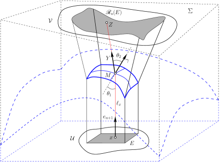
Figure 1. The blue doted lines confine the boundary of media $\rm I$.

If $\gamma$ is the unit normal at $M=(x,u(x))\in\mathbb{R}^{n+1}$ where $\ell_{x}$ strikes $\Gamma_{u}$ then from the refraction law we have

(1.1) $$\frac{\sin\theta_{1}}{\sin\theta_{2}}=\frac{n_{2}}{n_{1}},$$

where $n_{1},n_{2}$ are the refractive indices of the media I and II respectively, dissevered by the interface $\Gamma_{u}$, $\theta_{1}$ and $\theta_{2}$ are the angles between $\ell_{x}$ and $\gamma$, and between $Y$ and $\gamma$, respectively, see Figure 1.

Suppose that the intensity of light on $\mathcal{U}$ is $f\geq 0$ and let $\mathcal{V}$ be the set of points where the refracted rays strike the receiver $\Sigma$. Denote by $g\geq 0$ the gain intensity on $\mathcal{V}$. For each $\mathcal{U}^{\prime}\subset\mathcal{U}$ let $\mathcal{V}^{\prime}$ be the set of points where the rays, issued from $\mathcal{U}^{\prime}$ and refracted off $\Gamma_{u}$, strike $\Sigma$. Thus $u$ generates the refractor mapping

$$Z_{u}:\mathcal{U}\longrightarrow\mathcal{V}$$

and the illuminated domain on $\Sigma$, corresponding to $\mathcal{U}^{\prime}\subset\mathcal{U}$, is $\mathcal{V}^{\prime}=Z_{u}(\mathcal{U}^{\prime})$. If $\Gamma_{u}$ is a perfect refractor, then one would have the energy balance equation (in local form)

(1.2) $$\int\limits_{\mathcal{U}^{\prime}}f=\int\limits_{\mathcal{V}^{\prime}=Z_{u}(\mathcal{U}^{\prime})}g.$$

The main problem that we are concerned with is formulated below:

Problem

Assume that we are given a smooth surface $\Sigma$ in $\mathbb{R}^{n+1}$, a pair of bounded smooth domains $\mathcal{U}\subset\Pi=\{X\in\mathbb{R}^{n+1}:X^{n+1}=0\}$ and $\mathcal{V}\subset\Sigma$ and a pair of nonnegative, integrable functions $f:\mathcal{U}\to\mathbb{R}$ and $g:\mathcal{V}\to\mathbb{R}$ such that the energy balance condition holds

(1.3) $$\int_{\mathcal{U}}f=\int_{\mathcal{V}}gd\mathcal{H}^{n}.$$

Find a function $u:\mathcal{U}\to\mathbb{R}$ such that the following two conditions are fulfilled

(1.6) $$\left\{\begin{array}[]{lll}\int\limits_{\mathcal{U}^{\prime}}f=\int\limits_{Z_{u}(\mathcal{U}^{\prime})}g,\ \mbox{\it for\ any\ measurable}\ \mathcal{U}^{\prime}\subset\mathcal{U}\\ Z_{u}(\mathcal{U})=\mathcal{V}.\end{array}\right.$$

Problems of this kind appear in geometric optics [14] page 315. In the 17th century Descartes posed a similar problem with target set $\mathcal{V}$ being a single point, say $\mathcal{V}=\{Z_{0}\}$. It was observed that the ellipsoids and hyperboloids of revolution with focal axis parallel to $e_{n+1}$ will solve this problem if $Z_{0}$ is one of the foci. The case of general target $\mathcal{V}$ can be treated via approximation argument, namely by constructing a solution from ellipsoids or hyperboloids for finite set $\mathcal{V}=\{Z_{1},\dots,Z_{m}\}$ and then letting $m\rightarrow\infty$. Moreover, the eccentricity of these surfaces is fixed and determined by the refractive indices $n_{1}$ and $n_{2}$. To see this we take advantage of some well-known facts from geometric optics and record them here for further reference, see [19]. Let $H(x)=Z^{n+1}-a\varepsilon-\frac{a}{b}\sqrt{b^{2}+|x-x_{0}|^{2}}$ be the lower sheet of a hyperboloid of revolution with focal axis passing through the point $x_{0}\in\mathcal{U}$ and parallel to $e_{n+1}$, see Section 8. Similarly, we define the lower half of an ellipsoid of revolution $E(x)=Z^{n+1}-a\varepsilon-\frac{a}{b}\sqrt{b^{2}-|x-x_{0}|^{2}}$. If $n_{1}$ and $n_{2}$ are the refractive indices of media I and II respectively then

(1.9) $$\varepsilon=\frac{n_{1}}{n_{2}}=\frac{\sin\theta_{2}}{\sin\theta_{1}}=\left\{\begin{array}[]{lll}\frac{\sqrt{a^{2}-b^{2}}}{a}<1\ \ \textrm{for ellipsoids},\\ \frac{\sqrt{a^{2}+b^{2}}}{a}>1\ \ \textrm{for hyperboloids}.\end{array}\right.$$

Here $\varepsilon$ is the eccentricity, see [19]. Since $\varepsilon$ is fixed we can drop the dependence of $E$ and $H$ from $b=a\sqrt{|\varepsilon^{2}-1|}$ and take

(1.10) $$E(x,a,Z)=Z^{n+1}-a\varepsilon-a\sqrt{1-\frac{(x-z)^{2}}{a^{2}(1-\varepsilon^{2})}}, \quad\rm{if}\ \varepsilon<1,$$

(1.11) $$H(x,a,Z)=Z^{n+1}-a\varepsilon-a\sqrt{1+\frac{(x-z)^{2}}{a^{2}(\varepsilon^{2}-1)}}, \quad\rm{if}\ \varepsilon>1.$$

We also define the constant

(1.12) $$\kappa=\frac{\varepsilon^{2}-1}{\varepsilon^{2}}$$

which will prove to be useful, in a number of computation to follow.

2. Main theorems

Let $\Sigma$ be the receiver surface defined implicitly

(2.1) $$\Sigma=\{Z\in\mathbb{R}^{n+1}:\psi(Z)=0\}$$

where $\psi:\mathbb{R}^{n+1}\to\mathbb{R}$ is a smooth function. If $u\in C^{2}(\mathcal{U})$ then the first condition in (1.6), after using change of variables, results a Monge-Ampère type equation for $u$, whereas the second one plays the role of boundary condition for $u$. More precisely we have the following

Theorem A.

Let $u\in C^{2}(\mathcal{U})$ be a solution to (1.6). Then

• $Y=\varepsilon\left(\frac{\kappa Du}{1+q},1-\frac{\kappa}{1+q}\right)$ is the unit direction of refracted ray,

• $u$ solves the equation

  (2.2) $$\left|\text{det}\left[\frac{q+1}{t\varepsilon\kappa}\left\{{\rm{Id}}-\kappa\varepsilon^{2}Du\otimes Du\right\}+D^{2}u\right]\right|=\left|-\varepsilon q\left[\frac{q+1}{t\varepsilon\kappa}\right]^{n}\frac{\nabla\psi\cdot Y}{|\nabla\psi|}\frac{f}{g}\right|,$$

where

(2.3) $$q(x)=\sqrt{1-\kappa(1+|Du|^{2})},\quad\kappa=\frac{\varepsilon^{2}-1}{\varepsilon^{2}}$$

and $t$ is the stretch function defined in (4.11) via an implicit relation $\psi(x+e_{n+1}u(x)+Yt)=0$.

If the receiver $\Sigma$ is a plane then taking $\psi(Z)=Z\cdot\xi+\xi_{1}$ we find that $t=-[Y\cdot\xi_{0}]^{-1}(x+u(x)e_{n+1}+\xi_{1})$. In particular for the horizontal plane $X^{n+1}=m$, with some constant $m>0$, one has

$$t=\frac{m-u}{Y^{n+1}}=(m-u)\frac{q+1}{\varepsilon(1-\kappa+q)}.$$

Quadric $\Sigma$ is another example of receiver for which $t$ can be computed explicitly. In general $t$ is a function of $x,u(x)$ and $Du(x)$ which may not have simple explicit form. However, in terms of applications the case of planar receiver is of particular interest, since the flat screens are easy to construct. The method of the stretch function was introduced in [12, 13] to treat the near-field reflection problem. The equation for a near-field refraction problem with point source is derived in [6], [10].

Next, we need to introduce the notion of weak solution of (2.2). It will allow us to develop the existence theory along the lines of the classical Monge-Ampère equation. To this end, we say that $u:\mathcal{U}\to\mathbb{R}$ is upper (resp. lower) admissible with respect to $\mathcal{V}$ if for any $x\in\mathcal{U}$ there is a hyperboloid $H(\cdot,a,Z)$ (resp. ellipsoid $E(\cdot,a,Z)$) with focus $Z\in\mathcal{V}$ such that $H(\cdot,a,Z)$ (resp. $E(\cdot,a,Z)$) touches $u$ from above (resp. below) at $x$. Such $H(\cdot,a,Z)$ (resp. $E(\cdot,a,Z)$) is called supporting hyperboloid (resp. ellipsoid) of $u$ at $x$. To fix the ideas we consider the class of upper admissible function and denote it by $\overline{\mathbb{W}}_{\rm H}(\mathcal{U},\mathcal{V})$. The class of lower admissible functions is denoted by $\underline{\mathbb{W}}_{\rm E}(\mathcal{U},\mathcal{V})$. For each $u\in\overline{\mathbb{W}}_{\rm H}(\mathcal{U},\mathcal{V})$ we define the mapping $\mathscr{S}_{u}:\mathcal{V}\to\mathcal{U}$ by

$$\mathscr{S}_{u}(Z)=\{x\in\mathcal{U}:\exists a>0\ \mbox{such \ that}\ H(\cdot,a,Z)\ \mbox{is\ a \ supporting \ hyperboloid\ of}\ u\ \mbox{at}\ x\},$$

and take

$$\beta_{u,f}(E)=\int_{\mathscr{S}_{u}(E)}f(x)dx,\quad E\subset\mathcal{V}.$$

Furthermore, we also consider the mapping $\mathscr{R}_{u}:\mathcal{U}\to\mathcal{V}$ defined by

$$\mathscr{R}_{u}(x)=\{Z\in\mathcal{V}:\mbox{there \ is\ a \ supporting \ hyperboloid}\ H(\cdot,a,Z)\ \mbox{ of}\ u\ \mbox{at}\ x\}$$

and associate the following set function

$$\alpha_{u,g}(E)=\int_{\mathscr{R}_{u}(E)}gd\mathcal{H}^{n},\quad E\subset\mathcal{V}.$$

Notice that for smooth $u$, the mapping $\mathscr{S}_{u}$ is the inverse of $\mathscr{R}_{u}$.

With the aid of these set functions $\alpha_{u,g}$ and $\beta_{u,f}$ we can introduce two notions of weak solution to (1.6), called $A$ and $B$ type weak solutions, respectively. It is not hard to see that $\beta_{u,f}$ is in fact $\sigma$-additive measure, while for $\alpha_{u,g}$ it is less obvious. Towards proving this the major obstruction is to show that $\mathscr{R}_{u}$ is one-to-one modulo a set of vanishing $\mathcal{H}^{n}$ measure on $\Sigma$. This is circumvented by introducing the Legendre-like transformation $v(z)$ of an admissible function $u(x)$ in Section 11 defined as an upper envelope of some function of $\text{dist}(Z,X)$ for $Z\in\mathcal{V}$ and $X\in\mathcal{U}$. In order to infer that $v(z)$ is semi-concave (which in turn will lead to $\sigma$-additivity of $\alpha_{u,g}$) we assume that (2.5) is fulfilled. That done, one can show that an $A$-type weak solution exists in the sense of Definition 11.2. Note that once we found the Legendre-like transformation then our problem can be treated as a prescribed Jacobian type equation discussed in [24]. However one still has to check all conditions formulated there in order to trigger the theory. Furthermore, the construction of locally smooth solution for (1.6) is very complicated and require a careful analysis of Dirichlet’s problem. This issues are addressed in Lemma 10.2 and Section 13.

If, for a moment, we take the existence of $A$-type weak solution for granted, the question about its regularity is even more complex. To set stage for the weak solutions we assume that $\Sigma=\{Z\in\mathbb{R}^{n+1}:\psi(Z)=0\}$ and $\psi:\mathbb{R}^{n+1}\to\mathbb{R}$ being a smooth function. Clearly, some conditions must be imposed on $\psi$ to guarantee, among other things, that the right hand side of the equation (2.2) is well defined, at least for smooth solutions.

To this end we enlist the following conditions to be used in the construction of weak solutions and proving their smoothness.

(2.4) $$\nabla\psi(Z)\cdot(X-Z)>0\quad\forall X\in(\mathcal{U}\times[0,m_{0}]),\forall Z\in\Sigma\ {\rm and\ for\ some\ large\ constant}\ m_{0}>0,$$

(2.5) $$\text{dist}(\mathcal{U},\mathcal{V})>0,$$

(2.6) $$\mathcal{V}\ {\rm is}\ R-{\rm convex\ with\ respect\ to}\ \mathcal{U},\ {\rm see\ Definition}\ \ref{def-R-conv},$$

(2.7) $$f,g>0,$$

(2.8) $$\frac{1}{t}\left[\frac{t\varepsilon\kappa}{q+1}\right]^{2}{\rm II}+\frac{\kappa}{q}\frac{\psi_{n+1}}{|\nabla\psi|}\left({\rm{Id}}+\kappa\frac{p\otimes p}{q^{2}}\right)<0,\quad{\rm if}\ \kappa>0,$$

where $\rm II$ is the second fundamental form of $\Sigma$ and $p=Du(x)$. The subdomain of $\mathcal{U}\times[0,\infty)$ where (2.4)-(2.8) are simultaneously satisfied is called the regularity domain $\mathcal{D}$.

It is worthwhile to explain the meaning of these conditions: the first one (2.4) means that the reflected rays do not strike $\Sigma$ tangentially, otherwise $\Sigma$ would not detect the gain intensity at the tangential points, i.e. at the points where $\nabla\psi(Z)\cdot(X-Z)=0$. On the technical level, however, it allows to apply the inverse function theorem to recover the stretch function $t=t(x,u,Du)$. It is worth pointing out that (2.4) holds for a large class of surfaces $\Sigma$. To see this it is enough to notice that there is a positive constant $c(\varepsilon)$, depending only on $\varepsilon$ such that $Y^{n+1}\in[c(\varepsilon),1]$. In other words the unit directions $Y$ of refracted rays remain within the cone $c(\varepsilon)\leq Y^{n+1}\leq 1$. Indeed,if $u$ is differentiable at $x$ then $Y^{n+1}(x)=\varepsilon[1+(\sqrt{\cos^{2}\theta_{1}-\kappa}-\cos\theta_{1})\gamma^{n+1}]$ from refraction law, see (4.5) and Figure 1. Here $\kappa=1-\varepsilon^{-2}$. If $u$ is not differentiable at $x$, we interpret $\gamma$ as one of the normals of supporting planes of admissible $u$ at $x\in\mathcal{U}$ since $u$ is concave (resp. convex) if $u$ is upper (resp. lower) admissible, see Section 8. Thus if $p\in\partial u(x)$, where $\partial u$ is the subdifferential of $u$ at $x$, then $\gamma=\left(\frac{p}{\sqrt{1+|p|^{2}}},\frac{1}{\sqrt{1+|p|^{2}}}\right)$ and $\cos\theta_{1}=\frac{1}{\sqrt{1+|p|^{2}}}$. Consequently if $u$ is lower admissible then $Y^{n+1}\geq\varepsilon$ if $\kappa<0$, i.e. $\varepsilon<1$ and hence $c(\varepsilon)=\varepsilon<1$. On the other hand if $\kappa>0$ then for any $u\in\mathbb{H}(\mathcal{U},\mathcal{V})$ we have

(2.9) $$\sup_{\mathcal{U}}|Du|<\frac{1}{\sqrt{\varepsilon^{2}-1}}\quad{\rm if}\ \kappa=\frac{\varepsilon^{2}-1}{\varepsilon^{2}}>0.$$

This simply follows from the fact that supporting hyperboloids control the magnitude of the gradient of $u$, see Lemma 8.1. But in its turn $|DH|$, for any hyperboloid $H$ given by (1.11), satisfies the estimate (2.9). Because $\gamma^{n+1}=\cos\theta_{1}=\frac{1}{\sqrt{1+|p|^{2}}}$ (see Figure 1 and the derivation of (4.8)) and $|p|<\frac{1}{\sqrt{\varepsilon^{2}-1}}$ we infer that

$$(\sqrt{\cos^{2}\theta_{1}-\kappa}-\cos\theta_{1})\gamma^{n+1}=\frac{-\kappa}{\sqrt{\cos^{2}\theta_{1}-\kappa}+\cos\theta_{1}}\gamma^{n+1}>-\kappa$$

and consequently $Y^{n+1}>\varepsilon(1-\kappa)=\varepsilon^{-1}<1$. Thus for $\varepsilon>1$ we can take $c(\varepsilon)=\varepsilon^{-1}$. From here we see that (2.4) holds for any horizontal receiver $Z^{n+1}=m$, for large $m>0$. More generally if $\Sigma$ is concave in $Z^{n+1}$ direction and the normal mapping of $\Sigma$ is strictly inside of the cone $c(\varepsilon)<Y^{n+1}$ on the unit sphere then (2.4) holds true. This leads to the following cone condition for the unit directions of refracted rays

(2.10) $$0<c(\varepsilon)\leq Y^{n+1}\leq 1.$$

The second condition (2.5) assures that the Legendre-like transformation $v(z)$ for an admissible function $u$ is well defined as an envelope of $C^{1}$ smooth functions, in particular $v(z)$ is semi-concave and hence differentiable almost everywhere, see Section 11. This yields that $\alpha_{u,g}$ is a Radon measure.

The next two conditions (2.6) and (2.7) assure that $B$-type solution is also of $A$-type and therefore one gets the existence of $A$-type weak solutions in some indirect way using the methods of [4], [26]. That done, we can approximate $\mathcal{V}$ by R-convex domains and show the existence of $A$-type weak solutions without assuming (2.6), see Theorem C4.

Last condition (2.8), which is crucial for regularity of weak solutions, deserves special attention because it is the most sophisticated one. In fact the next theorem is entirely devoted to the verification of (2.8).

Theorem B.

Let $u$ be a $C^{2}(\mathcal{U})$ solution of (2.2) and II be the second fundamental form of $\Sigma=\{Z\in\mathbb{R}^{n+1}:Z^{n+1}=\varphi(z)\}$. Let $\kappa>0,{\rm II}<0$ then there is a constant $\lambda>0$ such that if $\text{dist}(\mathcal{U},\mathcal{V})>\lambda$ then (2.8). Furthermore, for $\kappa<0,{\rm II}>0$ there is a constant $\hat{\lambda}>0$ such that if $\text{dist}(\mathcal{U},\mathcal{V})>\hat{\lambda}$ then the opposite inequality in (2.8) holds for all $x\in\mathcal{U}$.

If $\Sigma$ is a graph, say $Z^{n+1}=\varphi(z)$ then (2.8) can be rewritten as

$$\frac{1}{t}\left[\frac{t\varepsilon\kappa}{q+1}\right]^{2}D^{2}\varphi+\frac{\kappa}{q}\left({\rm{Id}}+\kappa\frac{p\otimes p}{q^{2}}\right)<0,\quad{\rm if}\ \kappa>0.$$

In lieu of (2.10) this assumption on $\Sigma$ is not restrictive. In addition, Theorem B suggests that it is convenient to think of $\Sigma$ as an unbounded convex (resp. concave) surface without boundary if $\kappa<0$ (resp. $\kappa>0$) by extending $\varphi$ to $\mathbb{R}^{n}$ as a convex function $\widetilde{\varphi}$ such that $\varphi(z)\to\pm\infty$ as $|z|\to\infty$. We will take advantage of such extension of $\varphi$ (and hence $\Sigma$) in Section 8.4 and Lemma 10.2, see also Remark 7.1.

Now we are ready to formulate our main existence result.

Theorem C.

• If $f,g\geq 0$ and (1.3) and (2.4) hold then there is a $B$-type weak solution provided that the condition below

  (2.11) $$Z^{n+1}\geq\left[\frac{2}{\varepsilon-1}+\frac{1}{\sqrt{\varepsilon^{2}-1}}\right]\rho(z)$$

  is satisfied. Here $\rho(z)=\inf\{R>0:\mathcal{U}\subset B_{R}(z)\}$ is the maximal visibility radius from $z\overset{def}{=}\widehat{Z}\in\widehat{\mathcal{V}}$,

• if (2.4) and (2.5) hold then $\alpha_{u,g}$ is countably additive,

• if (2.4)-(2.6), (2.11) hold and $f\geq 0$ while $g>0$ then $B$-type weak solution is also of $A$ type,

• if we remove the $R-$convexity assumption but require the positivity of densities (2.7) and (2.4)-(2.5), (2.11) then again any $B$-type weak solution is also of $A$-type.

The proof of Theorem C1 is by polyhedral approximation and utilising the confocal expansion of hyperboloids as described in Section 8.4. In this regard the condition (2.11) in Theorem C1 says that one can construct a $B$-type weak solution if there is sufficient span between $\Pi$ and $\Sigma$. The existence of $B$-type weak solutions, constructed from an envelope of ellipsoids of revolution can be found in [7].

Our last result concerns with the smoothness of $A$-type weak solutions. We use the well-known method of comparing the mollified weak solution with that of Dirichlet’s problem to the slightly modified equation in a small ball $B$. To this end one first has to obtain $C^{2,\alpha},\alpha\in(0,1]$ estimates in $\overline{B}$ for the solutions of mollified equations and after that making sure that uniform $C^{2}$ estimates hold in, say, $\frac{1}{2}B$. Then passing to limit and using the comparison principle the result will follow. The construction of weak solutions to Dirichlet’s problem is based on Perron’s method and follows the approach developed by Xu-Jia Wang in [27] where a far field reflector design problem is studied. Our research is inspired by [27] and subsequent developments in [12], [13] [11]. For more recent results on this problem see [15]. The global $C^{2}$ estimates for the solution of Dirichlet’s problem for the regularised equation follow from [9] whereas the local uniform estimates in $\frac{1}{2}B$ are established in [18], see also [16] for the global regularity of near field reflector problem with point source of a light. Thus we have the following theorem

Theorem D.

Let $f,g$ be $C^{2}$ smooth functions such that $\lambda\leq f,g\leq\Lambda$ for some constants $\Lambda>\lambda>0$ and the conditions (2.4)- (2.8) are satisfied. Then $A$-type weak solutions of (1.6) are locally $C^{2}$ regular in $\mathcal{U}$.

The conditions (2.4)- (2.8) cannot be relaxed as one may easily construct counterexamples to regularity in the spirit of those in [12], [13]. For instance let us examine (2.6) (see also Remark 12.3), if we take a two point target $\mathcal{V}=\{Z_{1}\}\cup\{Z_{2}\}$ and consider $H(x)=\min[H(x,a_{1},Z_{1}),H(x,a_{2},Z_{2})]$ such that these hyperboloids $H(\cdot,a_{i},Z_{i}),i=1,2$ have non empty intersection over $\mathcal{U}$. Then approximating $\mathcal{V}$ by smooth R-convex sets $\mathcal{V}_{t}$ we obtain a sequence of admissible functions $H_{t}$, solving the refractor problem with target $\mathcal{V}_{t}$, and converging to $H$ as $t\to 0$. But if $t$ is sufficiently close to 0 then $H_{t}$ cannot remain $C^{1}$ smooth because otherwise the limit $H$ would also be $C^{1}$ which is impossible., see [12] for more discussion on such constructions. We would also like to point out a recent paper of Gutiérred and Tournier [8] where the authors study the local $C^{1,\alpha}$ regularity of reflector/refractor problems without using the explicit form of the equation. There one can find a detailed account of the case when the supporting functions are ellipsoids of revolution. Our work contributes in this direction only by deriving the explicit equation for general receiver $\Sigma$ and establishing a simple form of the corresponding regularity condition (involving the second fundamental form of $\Sigma$) for the existence of $C^{2}$ smooth solutions, see Section 7.3. In this paper, however, we mainly focus on the case when the supporting functions are the hyperboloids of revolution.

The rest of the paper is organized as follows: in the next section we derive the main formulae. Then we prove Theorem A in Section 4. The main result there is Proposition 5.1 from which the proof of Theorem A easily follows. Section 5 contains some preliminary discussion on the condition (2.8) and after that in Section 6 we give the proof of Theorem B. The admissible functions are introduced in Section 7 where we also exhibit some interesting properties of hyperboloids of revolution, notably the dual admissibility and confocal expansion. Employing the polyhedral approximation technique and weak convergence of measures $\beta_{u,f}$ we prove Theorem C1 in Section 8. The first direct application of (2.8) is given in Lemma 10.1, which is G. Loeper’s geometric interpretation of the A3 condition from [18]. A direct consequence of this is Lemma 10.2 stating that a suitable dilation of an admissible function by a paraboloid of revolution can be approximated via smooth subsolutions of (2.2). This is a crucial ingredient in the proof of Theorem D. Next we introduce the Legendre-like transformation of an admissible $u$ and conclude Theorem C2. The proofs of Theorem C3-4 follow from a comparison of $A$ and $B$ type weak solutions by extending the results of Luis Caffarelli [4] and John Urbas [26] for the classical Monge-Ampère equation to (2.2). This is done in Section 11. The last two sections are devoted to the study of the higher regularity of $A$-type weak solutions. We follow the classical approach developed by A. Pogorelov for the classical Monge-Ampère equation, see [20], [21]. Therefore, we first prove the solvability of weak Dirichlet’s problem when the boundary data is given as the trace of an $A$-type weak subsolution. That done, the uniqueness follows from comparison principle stated in Proposition 13.1. Finally in Section 13 we give the proof of our main regularity result, Theorem D.

3. Notations

$C,C_{0},C_{n},\cdots$	generic constants,
$\Pi$	$\Pi=\mathbb{R}^{n}\times\{0\}$,
$\overline{\Omega}$	closure of a set $\Omega$,
$\partial\Omega$	boundary of a set $\Omega$,
$\widehat{\Omega}$	the projection of $\Omega\subset\mathbb{R}^{n+1}$ on $\Pi$,
$\widehat{X}$	$(x_{1},x_{2},\dots,x_{n},0)$ projection of $X=(x_{1},x_{2},\dots,x_{n},x_{n+1}),$
$\varepsilon$	eccentricity,
$\kappa$	$\kappa=\frac{\varepsilon^{2}-1}{\varepsilon^{2}}$,
$\mathcal{H}^{n}$	$n$-dimensional Hausdorff measure on $\Sigma$,
$\partial_{i}$	partial derivate with respect to $x_{i}$ variable,
$Du$	the gradient of a function $u$,
$\rho(z)$	$\inf\{R>0:\mathcal{U}\subset B_{z}(R)\}$ is the maximal visibility radius from $z\overset{def}{=}\widehat{Z}\in\widehat{\mathcal{V}}$,
$q$	see (2.3),
$\mathbb{H}(\mathcal{U},\Sigma)$	the class of hyperboloids of revolution with focal axis parallel to $Z^{n+1}$ and upper focus on $\Sigma$,
$\mathbb{H}^{+}_{a_{0}}(\mathcal{U},\mathcal{V})$	hyperboloids from $\mathbb{H}(\mathcal{U},\mathcal{V})$ which are nonnegative in $\mathcal{U}$ and $a>a_{0}$ for some fixed $a_{0}$,
$\overline{\mathbb{W}}_{\rm H},\underline{\mathbb{W}}_{\rm E}$	upper and lower admissible functions, see Lemma 8.1,
$\overline{\mathbb{W}}_{\rm H}^{0}(\mathcal{U},\mathcal{V})$	polyhedral admissible functions.

4. Main formulae

In this section we derive the Monge-Ampère type equation (2.2) manifesting the energy balance condition (1.2) in the refractor problem (1.6), see Introduction.

4.1. Computing $Y$

We first compute the unit direction of the refracted ray. Denote by $\gamma$ the unit normal to the graph of $u$, that is

(4.1) $$\gamma=\frac{(-D_{1}u,\dots,-D_{n}u,1)}{\sqrt{1+|Du|^{2}}}.$$

Since $\ell_{x},Y$ and $\gamma$ lie in the same hyperplane we have

(4.2) $$Y=\mathpzc Ae_{n+1}+\mathpzc B\gamma,$$

for some coefficients $\mathpzc A$ and $\mathpzc B$. Computing the scalar products $Y\cdot\gamma$ and $Y\cdot e_{n+1}$ we obtain the following equations (cf. (1.1))

$$\left\{\begin{array}[]{ll}\cos\theta_{2}=\mathpzc A\cos\theta_{1}+\mathpzc B,\\ \cos{(\theta_{1}-\theta_{2})}=\mathpzc A+\mathpzc B\cos\theta_{1}.\end{array}\right.$$

Multiplying the first equation by $\cos\theta_{1}$ and subtracting from the second one we conclude

$$\mathpzc A=\frac{\sin\theta_{2}}{\sin\theta_{1}},\hskip 56.9055pt\mathpzc B=\cos\theta_{2}-\mathpzc A\cos\theta_{1}.$$

Recalling our notations

(4.4) $$\kappa=\frac{\varepsilon^{2}-1}{\varepsilon^{2}},\qquad\varepsilon=\frac{n_{1}}{n_{2}},$$

we see that $\mathpzc A=\varepsilon$. Furthermore

$$n_{2}^{2}-n_{2}^{2}\cos^{2}\theta_{2}=n_{2}^{2}\sin^{2}\theta_{2}=n_{1}^{2}\sin^{2}\theta_{1}=n_{1}^{2}-n_{1}^{2}\cos^{2}\theta_{1}.$$

Dividing both sides of this identity by $n_{2}^{2}$ we obtain

$$\cos^{2}\theta_{2}=\varepsilon^{2}\cos^{2}\theta_{1}-(\varepsilon^{2}-1)=\varepsilon^{2}(\cos^{2}\theta_{1}-\kappa).$$

Therefore from $\mathpzc A=\varepsilon$ we conclude that $\mathpzc B=\varepsilon(\sqrt{\cos^{2}\theta_{1}-\kappa}-\cos\theta_{1})$. Returning to (4.2) we infer that the unit direction of the refracted ray is

(4.5) $$Y=\varepsilon\left(e_{n+1}+(\sqrt{\cos^{2}\theta_{1}-\kappa}-\cos\theta_{1})\gamma\right).$$

Notice that (4.1) implies

$$\cos\theta_{1}=\gamma\cdot e_{n+1}=\frac{1}{\sqrt{1+|Du|^{2}}}.$$

Consequently, denoting $Y=(Y^{1},Y^{2},\dots,Y^{n},Y^{n+1})$ and $y\in\mathbb{R}^{n}$, the projection of $Y$ onto $\Pi=\{X\in\mathbb{R}^{n+1}:X^{n+1}=0\}$, (i.e. $y=(Y^{1},Y^{2},\dots,Y^{n},0)$) we get

$$y = -\varepsilon\frac{Du}{\sqrt{1+|Du|^{2}}}\left(\sqrt{\cos^{2}\theta_{1}-\kappa}-\cos\theta_{1}\right)$$

$$= \frac{\varepsilon\kappa Du}{\sqrt{1+|Du|^{2}}}\frac{1}{\sqrt{\cos^{2}\theta_{1}-\kappa}+\cos\theta_{1}}$$

$$= \varepsilon\kappa\frac{Du}{\sqrt{1-\kappa(1+|Du|^{2})}+1}.$$

From this computation it follows that

(4.7) $$Y^{n+1}=\varepsilon\left(1-\frac{\kappa}{1+\sqrt{1-\kappa(1+|Du|^{2})}}\right).$$

Combining (4.1) and (4.7) we obtain

(4.8) $$Y=\varepsilon\left(\frac{\kappa Du}{1+\sqrt{1-\kappa(1+|Du|^{2})}},1-\frac{\kappa}{1+\sqrt{1-\kappa(1+|Du|^{2})}}\right).$$

If we use the notation $q(x)=\sqrt{1-\kappa(1+|Du|^{2})}$ (see (2.3)) then (4.8) takes the form

(4.9) $$Y=\varepsilon\left(\frac{\kappa Du}{1+q},1-\frac{\kappa}{1+q}\right).$$

Notice that by (4.8) $Y^{n+1}>0$ for all values of $\kappa$.

4.2. Stretch function

Assume that $\psi$ is a smooth function $\psi:\mathbb{R}^{n+1}\to\mathbb{R}$, and the receiver $\Sigma$ is given as the zero set of $\psi$

(4.10) $$\Sigma=\{Z\in\mathbb{R}^{n+1}:\psi(Z)=0\}.$$

Let us represent the mapping $Z:\mathcal{U}\to\Sigma$ in the following form

(4.11) $$Z=x+e_{n+1}u(x)+Yt,$$

where $t=t(x,u(x),Du(x))$ is determined from the equation $\psi(Z)=0$ and is called the stretch function. It is worthwhile to point out that the stretch function $t$ can be explicitly computed for a wide class of elementary surfaces. For instance, if $\Sigma$ is the horizontal plane $Z^{n+1}=m>0$ then from simple geometric considerations one finds that

$$t=\frac{m-u}{Y^{n+1}}$$

where $Y^{n+1}$ is given by (4.7).

In lemma to follow we denote by $z$ the projection of $Z$ onto $\Pi$, that is $z=x+ty$.

Lemma 4.1.

Let $dS_{\mathcal{U}}$ and $dS_{\mathcal{V}}$ be the area elements on $\mathcal{U}$ and $Z(\mathcal{U})=\mathcal{V}\subset\Sigma$ respectively and $z$ being the projection of $Z$ onto $\Pi=\{Z\in\mathbb{R}^{n+1}:Z^{n+1}=0\}.$ Then we have

$$J = \frac{dS_{\mathcal{V}}}{dS_{\mathcal{U}}}=\left|\begin{array}[]{cccc}Z_{1}^{1},&\cdots,&Z^{1}_{n},&\nu^{1}\\ \vdots&\ddots&\vdots&\vdots\\ Z^{n}_{1},&\cdots,&Z_{n}^{n},&\nu^{n}\\ Z^{n+1}_{1},&\cdots,&Z^{n+1}_{n},&\nu^{n+1}\\ \end{array}\right|$$

$$= -\frac{|\nabla\psi|}{\psi_{n+1}}\text{det}Dz,$$

where $\nu$ is the unit normal of $\Sigma$.

Proof. The first equality in (4.1) follows from the change of variables formula. Differentiating the equality $\psi(Z)=0$ by $x_{i}$ we have that

$$\partial_{i}Z^{n+1}=-\frac{1}{\partial_{n+1}\psi}\sum\limits_{k=1}^{n}\partial_{i}z^{k}\partial_{z_{k}}\psi.$$

Using this identity we multiply $j$-th row of matrix in (4.1) by $\partial_{z_{j}}\psi$ and subtract it from the $(n+1)$st row in order to get

$$\text{det}\left|\begin{array}[]{cccc}Z_{1}^{1},&\cdots,&Z_{n}^{1},&\nu_{1}\\ \vdots&\ddots&\vdots&\vdots\\ Z^{n}_{1},&\cdots,&Z^{n}_{n},&\nu_{n}\\ Z^{n+1}_{1},&\cdots,&Z^{n+1}_{n},&\nu_{n+1}\\ \end{array}\right| = -\frac{1}{\psi_{n+1}}\text{det}\left|\begin{array}[]{cccc}Z_{1}^{1},&\cdots,&Z_{n}^{1},&\nu_{1}\\ \vdots&\ddots&\vdots&\vdots\\ Z^{n}_{1},&\cdots,&Z^{n}_{n},&\nu_{n}\\ \sum\limits_{k=1}^{n}\partial_{1}z^{k}\partial_{z_{k}}\psi,&\cdots,&\sum\limits_{k=1}^{n}\partial_{n}z^{k}\partial_{z_{k}}\psi,&-\psi_{n+1}\nu_{n+1}\\ \end{array}\right|$$

$$= -\frac{1}{\psi_{n+1}}\text{det}\left|\begin{array}[]{cccc}Z_{1}^{1},&\cdots,&Z_{n}^{1},&\nu_{1}\\ \vdots&\ddots&\vdots&\vdots\\ Z^{n}_{1},&\cdots,&Z^{n}_{n},&\nu_{n}\\ 0,&\cdots,&0,&-\sum\limits_{k=1}^{n+1}\psi_{k}\nu_{k}\\ \end{array}\right|.$$

Finally noting that $\nu=\frac{\nabla\psi}{|\nabla\psi|}$ the desired identity follows.∎

Lemma 4.2.

Let $C\in\mathbb{R}$ and $\xi,\eta\in\mathbb{R}^{n}$. Consider the matrix $\mu={\rm{Id}}+C\xi\otimes\eta=\delta_{ij}+C\xi^{i}\eta^{j}$ where ${\rm{Id}}=\delta_{ij}$ is the identity matrix. Then the inverse matrix of $\mu$ is

$$\text{det}\mu = 1+C\xi\cdot\eta,$$

$$\mu^{-1} = {\rm{Id}}-\frac{C\xi\otimes\eta}{1+C(\xi\cdot\eta)}.$$

Here and henceforth ${\rm{Id}}$ is the identity matrix.

Proof.  Without loss of generality we assume that $\xi=e_{1}$ then $\text{det}\mu=1+C\eta^{1}$. As for the second identity, it is a partucal case of Sherman-Morrison formula. ∎

Finally, we derive a formula for the first order derivatives of the stretch function $t$. Let us differentiate the equation $\psi(Z)=0$ with respect to $x_{j}$ to get

$$\sum_{k=1}^{n}\psi_{k}(\delta_{kj}+t_{j}y^{k}+ty^{k}_{j})+\psi_{n+1}(u_{j}+t_{j}Y^{n+1}+tY^{n+1}_{j})=0.$$

From here we find

(4.18) $$t_{j}=-\frac{1}{\nabla\psi\cdot Y}[\psi_{j}+\psi_{n+1}u_{j}+t(\nabla\psi\cdot Y_{j})].$$

5. Proof of Theorem A

In this section we prove Theorem A. We begin with a computation for the matrix $Dz$, where $z$ is the projection of $Z$ on to $\Pi$.

Proposition 5.1.

Let $u\in C^{2}(\mathcal{U})$ and $Z$ be the corresponding refractor map, then with the same notations as in Lemma 4.1 we have

(5.1) $$Dz = \mu_{1}\mu_{2}\left[{\rm{Id}}-\kappa\varepsilon^{2}Du\otimes Du+\frac{t\kappa\varepsilon}{1+h}D^{2}u\right],$$

where

(5.2) $$\mu_{1}={\rm{Id}}-\frac{y\otimes(\widehat{\nabla}\psi-y\frac{\psi_{n+1}}{Y^{n+1}})}{\nabla\psi\cdot Y},\qquad\mu_{2}={\rm{Id}}+\kappa\frac{Du\otimes Du}{q(q+1)},$$

$q=\sqrt{1-\kappa(1+|Du|^{2})}$ and

(5.3) $$\widehat{\nabla}\psi=(\psi_{1},\dots,\psi_{n},0).$$

In order to prove Proposition 5.1 we will need the following

Lemma 5.1.

Let $z(x),x\in\mathcal{U}$ be the projection of the mapping $Z(x)$ onto $\Pi=\{X\in\mathbb{R}^{n+1}:X^{n+1}=0\}$. Then

(5.4) $$Dz=\mu_{1}\left({\rm{Id}}-y\otimes[y+DuY^{n+1}]+tDy\right)$$

where $\mu_{1}$ is defined by (5.2).

Proof. Introduce the matrix

(5.5) $$\mu_{0}=\delta_{ij}-y^{i}\frac{\psi_{j}+u_{j}\psi_{n+1}}{\nabla\psi\cdot Y}.$$

Using (4.18) and recalling $z=x+ty$ we compute

$$z^{i}_{j} = \delta_{ij}+t_{j}y^{i}+ty^{i}_{j}$$

$$= \delta_{ij}+ty^{i}_{j}-y^{i}\frac{1}{\nabla\psi\cdot Y}[\psi_{j}+\psi_{n+1}u_{j}+t(\nabla\psi\cdot Y_{j})]$$

$$= \underbrace{\delta_{ij}-y^{i}\frac{[\psi_{j}+u_{j}\psi_{n+1}]}{\nabla\psi\cdot Y}}_{\mu_{0}}+t\left[y^{i}_{j}-\frac{y^{i}(\nabla\psi\cdot Y_{j})}{\nabla\psi\cdot Y}\right]$$

$$= \mu_{0}+t\left[y^{i}_{j}-\frac{y^{i}(\nabla\psi\cdot Y_{j})}{\nabla\psi\cdot Y}\right].$$

In order to deal with the remaining matrix we recall that $(Y^{n+1})^{2}=1-|y|^{2}$ and hence $Y^{n+1}_{j}=-\frac{yy_{j}}{Y^{n+1}}$. Consequently, setting $\widehat{\nabla}\psi=(\psi_{1},\dots,\psi_{n},0)$ (see (5.3)) we infer

$$y^{i}_{j}-\frac{y^{i}(\nabla\psi\cdot Y_{j})}{\nabla\psi\cdot Y} = y^{i}_{j}-\frac{y^{i}}{\nabla\psi\cdot Y}\left(\widehat{\nabla}\psi\cdot y_{j}-\psi_{n+1}\frac{y\cdot y_{j}}{Y^{n+1}}\right)$$

$$= y^{i}_{j}-\frac{y^{i}}{\nabla\psi\cdot Y}\left[\left(\widehat{\nabla}\psi-\frac{\psi_{n+1}}{Y^{n+1}}y\right)y_{j}\right].$$

Combining (5) and (5) we obtain the following formula for $Dz$, written in intrinsic form

$$Dz = \mu_{0}+t\left[{\rm{Id}}-\frac{y\otimes\left(\widehat{\nabla}\psi-\frac{\psi_{n+1}}{Y^{n+1}}y\right)}{\nabla\psi\cdot Y}\right]Dy$$

$$= \mu_{0}+t\mu_{1}Dy$$

$$= \mu_{1}(\mu_{1}^{-1}\mu_{0}+tDy)$$

where the second equality follows from the definition of matrix $\mu_{1}$, see (5.2).

Next, we compute $\mu_{1}^{-1}$. From Lemma 4.2 and the identity $[Y^{n+1}]^{2}=1-|y|^{2}$ we get

$$\mu_{1}^{-1} = {\rm{Id}}+y\otimes\frac{\widehat{\nabla}\psi-\frac{\psi_{n+1}}{Y^{n+1}}y}{\nabla\psi\cdot Y-\left(\widehat{\nabla}\psi\cdot y-|y|^{2}\frac{\psi_{n+1}}{Y^{n+1}}\right)}$$

$$= {\rm{Id}}+\frac{Y^{n+1}}{\psi_{n+1}}y\otimes\left[\widehat{\nabla}\psi-\frac{\psi_{n+1}}{Y^{n+1}}y\right],$$

where the last equality follows from the observation

$$\nabla\psi\cdot Y-\left(\widehat{\nabla}\psi\cdot y-|y|^{2}\frac{\psi_{n+1}}{Y^{n+1}}\right) = \psi_{n+1}Y^{n+1}+(1-(Y^{n+1})^{2})\frac{\psi_{n+1}}{Y^{n+1}}$$

$$= \frac{\psi_{n+1}}{Y^{n+1}}.$$

It is convenient to rewrite this identity in the following form

(5.11) $$\left[\widehat{\nabla}\psi\cdot y-|y|^{2}\frac{\psi_{n+1}}{Y^{n+1}}\right]\frac{Y^{n+1}}{\psi_{n+1}}\frac{1}{\nabla\psi\cdot Y}=\frac{Y^{n+1}}{\psi_{n+1}}-\frac{1}{\nabla\psi\cdot Y}.$$

Consequently, we obtain

$$\mu_{1}^{-1}\mu_{0} = \left({\rm{Id}}+\frac{Y^{n+1}}{\psi_{n+1}}y\otimes\left[\widehat{\nabla}\psi-\frac{\psi_{n+1}}{Y^{n+1}}y\right]\right)\left({\rm{Id}}-y\otimes\frac{\widehat{\nabla}\psi+Du\psi_{n+1}}{\nabla\psi\cdot Y}\right)$$

$$= {\rm{Id}}-y\otimes\frac{\widehat{\nabla}\psi+Du\psi_{n+1}}{\nabla\psi\cdot Y}+\frac{Y^{n+1}}{\psi_{n+1}}y\otimes\left[\widehat{\nabla}\psi-\frac{\psi_{n+1}}{Y^{n+1}}y\right]-$$

$$-\left[\widehat{\nabla}\psi\cdot y-|y|^{2}\frac{\psi_{n+1}}{Y^{n+1}}\right]\frac{Y^{n+1}}{\psi_{n+1}}\frac{1}{\nabla\psi\cdot Y}\left\{y\otimes{\widehat{\nabla}\psi+Du\psi_{n+1}}\right\}.$$

Applying (5.11) to the last term in this computation we get

$$\mu_{1}^{-1}\mu_{0} = {\rm{Id}}-y\otimes\frac{\widehat{\nabla}\psi+Du\psi_{n+1}}{\nabla\psi\cdot Y}+\frac{Y^{n+1}}{\psi_{n+1}}y\otimes\left[\widehat{\nabla}\psi-\frac{\psi_{n+1}}{Y^{n+1}}y\right]-$$

$$-\left[\frac{Y^{n+1}}{\psi_{n+1}}-\frac{1}{\nabla\psi\cdot Y}\right]\left\{y\otimes{\widehat{\nabla}\psi+Du\psi_{n+1}}\right\}$$

$$= {\rm{Id}}+\frac{Y^{n+1}}{\psi_{n+1}}y\otimes\left[\widehat{\nabla}\psi-\frac{\psi_{n+1}}{Y^{n+1}}y\right]-$$

$$-\frac{Y^{n+1}}{\psi_{n+1}}\left\{y\otimes{\widehat{\nabla}\psi+Du\psi_{n+1}}\right\}$$

$$= {\rm{Id}}-y\otimes[y+Du\psi_{n+1}].$$

Plugging in the computed form of $\mu_{1}^{-1}\mu_{0}$ into (5) the result follows. ∎

5.1. Proof of Proposition 5.1

To finish the proof of Proposition 5.1, it remains to express $Dz$ through the Hessian $D^{2}u$. We have from (4.9)

(5.12) $$y = \varepsilon\kappa\frac{Du}{q+1},$$

(5.13) $$Y^{n+1} = \varepsilon\left(1-\frac{\kappa}{q+1}\right),$$

where $q=\sqrt{1-\kappa(1+|Du|^{2})}$, see (2.3). From the definition of $q$ we have $Dq=-\kappa DuD^{2}u/q$, thus

$$Dy = \varepsilon\kappa\left[{\rm{Id}}+\kappa\frac{Du\otimes Du}{q(q+1)}\right]\frac{D^{2}u}{q+1}$$

$$= \varepsilon\kappa\mu_{2}\frac{D^{2}u}{q+1},$$

where $\mu_{2}$ is the matrix in (5.2). Now Lemma 5.1 yields

$$Dz = \mu_{1}\left({\rm{Id}}-y\otimes[y+DuY^{n+1}]+t\varepsilon\kappa\mu_{2}\frac{D^{2}u}{q+1}\right)$$

$$= \mu_{1}\mu_{2}\left(\mu_{2}^{-1}\left\{{\rm{Id}}-y\otimes[y+DuY^{n+1}]\right\}+t\varepsilon\kappa\frac{D^{2}u}{q+1}\right)$$

$$= \mu_{1}\mu_{2}\left(\mu_{2}^{-1}\mathcal{M}+t\varepsilon\kappa\frac{D^{2}u}{q+1}\right)$$

where $\mathcal{M}={\rm{Id}}-y\otimes[y+DuY^{n+1}]$.

Using (5.12) we can further simplify the matrix $\mathcal{M}={\rm{Id}}-y\otimes[y+DuY^{n+1}]$ to get

$$\mathcal{M} = {\rm{Id}}-y\otimes(y+DuY^{n+1})$$

$$= {\rm{Id}}-\frac{\varepsilon^{2}\kappa^{2}}{(1+q)^{2}}Du\otimes Du-\frac{\varepsilon^{2}\kappa(1-\frac{\kappa}{1+q})}{1+q}Du\otimes Du$$

$$= {\rm{Id}}-\frac{\varepsilon^{2}\kappa}{1+q}Du\otimes Du.$$

By Lemma 4.2 we have for the inverse of $\mu_{2}$ (see (5.2))

$$\mu_{2}^{-1} = {\rm{Id}}-\frac{\kappa}{q^{2}+q+\kappa|Du|^{2}}Du\otimes Du$$

$$= {\rm{Id}}-\frac{\kappa}{1-\kappa+q}Du\otimes Du,$$

where the last equality follows from the definition of $q$, see (2.3). It remains to compute $\mu_{2}^{-1}\cal M$. From (5.1) and (5.1) we obtain

$$\mu_{2}^{-1}\mathcal{M} = \left[{\rm{Id}}-\frac{\kappa}{1-\kappa+q}Du\otimes Du\right]\left[{\rm{Id}}-\frac{\varepsilon^{2}\kappa}{1+q}Du\otimes Du\right]$$

$$= {\rm{Id}}+\left[I+II+III\right]Du\otimes Du$$

where

$$I = -\frac{\kappa}{1-\kappa+q},$$

$$II = -\frac{\varepsilon^{2}\kappa}{1+q},$$

$$III = \frac{\varepsilon^{2}\kappa^{2}|Du|^{2}}{(1+q)(1-\kappa+q)}.$$

It follows from (2.3) that $-\kappa|Du|^{2}=q^{2}-1+\kappa$, therefore

$$III=\frac{\varepsilon^{2}\kappa(-q^{2}+1-\kappa)}{(1+q)(1-\kappa+q)}.$$

Adding this to $II$ we have

$$II+III = \frac{\varepsilon^{2}\kappa}{1+q}\left[-1+\frac{-q^{2}+1-\kappa}{1-\kappa+q}\right]$$

$$= -\frac{q\varepsilon^{2}\kappa}{1-\kappa+q}.$$

Finally we compute the total sum

$$I+II+III = -\frac{\kappa}{1-\kappa+q}-\frac{q\varepsilon^{2}\kappa}{1-\kappa+q}$$

$$= -\frac{\kappa}{1-\kappa+q}\left[q\varepsilon^{2}+1\right]$$

$$= -\frac{\kappa}{1-\kappa+q}\left[\frac{q}{1-k}+1\right]$$

$$= -\frac{\kappa}{1-\kappa}$$

$$= -\kappa\varepsilon^{2},$$

where the last line follows from the definition of $\kappa$, see (4.4).

Returning to (5.1) and utilising these computations we get

$$Dz = \mu_{1}\mu_{2}\left[\mu_{2}^{-1}\mathcal{M}+t\varepsilon\kappa\frac{D^{2}u}{q+1}\right]$$

$$= \mu_{1}\mu_{2}\left[{\rm{Id}}-\kappa\varepsilon^{2}Du\otimes Du+t\varepsilon\kappa\frac{D^{2}u}{q+1}\right].$$

This finishes the proof of Proposition 5.1. ∎

5.2. Proof of Theorem A

Now we are ready to finish the proof of Theorem A. Let $u\in C^{2}(\mathcal{U})$ be a solution to the refractor problem (1.6) then from Proposition 5.1 we obtain

(5.17) $$\text{det}Dz=\text{det}\mu_{1}\text{det}\mu_{2}\left[\frac{t\varepsilon\kappa}{q+1}\right]^{n}\text{det}\left[\frac{q+1}{t\varepsilon\kappa}\left\{{\rm{Id}}-\kappa\varepsilon^{2}Du\otimes Du\right\}+D^{2}u\right].$$

By Lemma 4.2 and (2.3) we have

$$\text{det}\mu_{2}=1+\frac{\kappa|Du|^{2}}{q(q+1)}=\frac{1-\kappa+q}{q(q+1)}.$$

Similarly, we get

$$\text{det}\mu_{1}=\frac{\psi_{n+1}}{Y^{n+1}}\frac{1}{\nabla\psi\cdot Y}.$$

These in conjunction with (4.1) gives

$$\text{det}\left[\frac{q+1}{t\varepsilon\kappa}\left\{{\rm{Id}}-\kappa\varepsilon^{2}Du\otimes Du\right\}+D^{2}u\right] = \left[\frac{q+1}{t\varepsilon\kappa}\right]^{n}\frac{\text{det}Dz}{\text{det}\mu_{1}\text{det}\mu_{2}}$$

$$= -\frac{f}{g}\frac{\psi_{n+1}}{|\nabla\psi|}\left[\frac{q+1}{t\varepsilon\kappa}\right]^{n}\frac{1}{\text{det}\mu_{1}\text{det}\mu_{2}}$$

$$= -(\nabla\psi\cdot Y)\frac{Y^{n+1}}{|\nabla\psi|}\frac{q(q+1)}{1-\kappa+q}\left[\frac{q+1}{t\varepsilon\kappa}\right]^{n}\frac{f}{g}.$$

Finally, recalling (4.9) and substituting the value of $Y^{n+1}$ we see that

$$\text{det}\left[\frac{q+1}{t\varepsilon\kappa}\left\{{\rm{Id}}-\kappa\varepsilon^{2}Du\otimes Du\right\}+D^{2}u\right] = -(\nabla\psi\cdot Y)\frac{Y^{n+1}}{|\nabla\psi|}\frac{q(q+1)}{1-\kappa+q}\left[\frac{q+1}{t\varepsilon\kappa}\right]^{n}\frac{f}{g}$$

$$= -\varepsilon q\left[\frac{q+1}{t\varepsilon\kappa}\right]^{n}\frac{\nabla\psi\cdot Y}{|\nabla\psi|}\frac{f}{g}$$

and the proof of Theorem A is now complete. ∎

6. Existence of smooth solutions

In this section we will have a provisional discussion on the existence of smooth solutions to (2.2). Our main objective is to apply the available regularity theory for the Monge-Ampère type equations, stemming from seminal paper [18], in order to establish the regularity of weak solutions of the refractor problem.

We first rewrite the equation (5.2) in a more concise form. Let us introduce the following matrix

(6.1) $$G^{ij}=\frac{1}{t}(q+1)[\delta_{ij}-\kappa\varepsilon^{2}u_{i}u_{j}].$$

Here $q=\sqrt{1-\kappa(1+|Du|^{2})}$, see (2.3) and $t$ is the stretch function determined from implicit equation $\psi(x+e_{n+1}u+tY)=0$ as in Theorem A. Then the equation (5.2) transforms into

(6.2) $$\text{det}\left[-\frac{G}{\varepsilon\kappa}-D^{2}u\right] = |h(x,u,Du)|,\quad{\rm if}\ \kappa>0,\varepsilon>1\quad u\in C^{2}(\mathcal{U})\ {\rm and}\ -\frac{G}{\varepsilon\kappa}-D^{2}u\geq 0,\$$

(6.3) $$\text{det}\left[D^{2}u+\frac{G}{\varepsilon\kappa}\right] = |h(x,u,Du)|,\quad{\rm if}\ \kappa<0,\varepsilon<1\quad u\in C^{2}(\mathcal{U})\ {\rm and}\ \frac{G}{\varepsilon\kappa}+D^{2}u\geq 0$$

with

(6.4) $$h(x,u,Du)=-\varepsilon q\left[\frac{q+1}{t\varepsilon\kappa}\right]^{n}\frac{\nabla\psi\cdot Y}{|\nabla\psi|}\frac{f}{g}.$$

The existence of $C^{2}$ smooth solutions of (6.2) or (6.3) depend on the properties of the matrix $G$. Namely, it is shown in [18] that if we regard $G$ as a function of variable $p=Du$ then the condition

(6.5) $$-D^{2}_{p_{k}p_{l}}G^{ij}\xi_{i}\xi_{j}\eta_{k}\eta_{l}\ \begin{array}[]{lll}\leq-c_{0}|\xi|^{2}|\eta|^{2}&\textrm{if}\ \kappa>0\\ \geq c_{0}|\xi|^{2}|\eta|^{2}&\textrm{if}\ \kappa<0\end{array}\qquad\forall\xi,\eta\in\mathbb{R}^{n},\xi\perp\eta,$$

with $c_{0}$ being a positive constant, is sufficient to obtain a priori $C^{1,1}$ bounds for the smooth solutions.

It is noteworthy to point out that the condition (6.5) and the $C^{2}$ estimates were derived in [18] for the Monge-Ampère type equations with variational structure emerging in optimal transport theory. The method used there is based on comparing the weak solution with the smooth one in a small ball. To employ this method successfully in the outset of refractor problem we need to establish a comparison principle, suitable mollification of the weak solution and a priori estimated for the smooth solutions of Dirichlet’s problem in small balls.

The method outlined above gives the $C^{2}$ estimates for non-variational case as well, see [12, 13]. Therefore the local regularity result for the solutions to (6.2)-(6.3) with smooth $w$ will follow once the matrix $G$ verifies the condition (6.5). That done, the regularity of weak solutions reduces to the verification of the inequality (6.5) with some positive constant $c_{0}$.

The conditions imposed on the matrix in (6.2)-(6.3) involving the Hessian implies that the Monge-Ampère equation is degenerate elliptic. The weak formulation of degenerate ellipticity will be discussed in Section 11. Postponing the precise definition of weak solutions until then we would like to point out how the ellipticity of equation follows if we consider those $C^{2}$ solutions of (6.2) (resp. (6.3)) for which at every point $x\in\mathcal{U}$ there is a hyperboloid (resp. ellipsoid) of revolution $H(\cdot,a,Z)$ touching $u$ from above (reps. below) at $x$. Indeed, for $H(x)=\ell_{0}-\frac{a}{b}\sqrt{b^{2}+|x-x_{0}|^{2}}$ the matrix $\cal W_{H}=-\frac{G}{\varepsilon\kappa}+D^{2}H$ is identically zero. To see this we consider the case of planar receiver $\Sigma$ given as $X^{n+1}=m$ with $m>0$. Without loss of generality we take $x_{0}=0$. Then $H(0)=\ell_{0}-a$. On the other hand it follows from the definition of eccentricity $\varepsilon=\frac{\sqrt{a^{2}+b^{2}}}{a}$ that $\ell_{0}=m-a\varepsilon$, see Section 8. Next, a simple geometric reasoning yields the following explicit formula for the stretch function

(6.6) $$t=\frac{m-H}{Y^{n+1}}=\frac{c+\frac{a}{b}\sqrt{b^{2}+|x|^{2}}}{\varepsilon(1-\frac{\kappa}{q+1})}.$$

We have $DH=-\frac{a}{b}\frac{x}{\sqrt{b^{2}+|x|^{2}}}$. Consequently

(6.7) $$D^{2}H=-\frac{a}{b\sqrt{b^{2}+|x|^{2}}}\left({\rm{Id}}-\frac{x\otimes x}{b^{2}+|x|^{2}}\right).$$

Moreover, recalling (4.4) we obtain $\kappa=1-\frac{1}{\varepsilon^{2}}=\frac{b^{2}}{c^{2}}$ where $c=\sqrt{a^{2}+b^{2}}$. This gives

(6.8) $$q(x)=\frac{1}{\varepsilon}\frac{b}{\sqrt{b^{2}+|x|^{2}}},$$

in lieu of (2.3).

Thus combining these formulae for $t$ and $q$ we get from (6.1), (6.6) and (6.7)

$$\cal W_{H} = -\frac{G}{\varepsilon\kappa}-D^{2}H$$

$$= -\frac{q+1}{\kappa\varepsilon t}\left\{[\delta_{ij}-\kappa\varepsilon^{2}H_{i}H_{j}]+\frac{\kappa\varepsilon tD^{2}_{ij}H}{q+1}\right\}$$

$$= -\frac{q+1}{\kappa\varepsilon t}\left\{{\rm{Id}}-\bigg{[}\kappa\varepsilon^{2}\underbrace{\frac{a^{2}}{b^{2}}\bigg{]}\frac{x\otimes x}{b^{2}+|x|^{2}}}_{DH\otimes DH}+\frac{\kappa\varepsilon t}{q+1}\underbrace{\left[-\frac{a}{b\sqrt{b^{2}+|x|^{2}}}\left({\rm{Id}}-\frac{x\otimes x}{b^{2}+|x|^{2}}\right)\right]}_{D^{2}H}\right\}.$$

From the definition of $\kappa$ (1.12) it follows that $\kappa\varepsilon^{2}\frac{a^{2}}{b^{2}}=\frac{b^{2}}{c^{2}}\varepsilon^{2}\frac{a^{2}}{b^{2}}=1$ implying

$$\cal W_{H}=-\frac{q+1}{\kappa\varepsilon t}\left({\rm{Id}}-\frac{x\otimes x}{b^{2}+|x|^{2}}\right)\left\{1-\frac{\kappa\varepsilon t}{q+1}\left[\frac{a}{b\sqrt{b^{2}+|x|^{2}}}\right]\right\}.$$

Therefore, recalling (6.6) and (6.8) we easily compute

$$t = \frac{c+\frac{a}{b}\sqrt{b^{2}+|x|^{2}}}{\varepsilon(1-\frac{\kappa}{h+1})}=(q+1)\frac{c+\frac{a}{b}\sqrt{b^{2}+|x|^{2}}}{\varepsilon(q+1-\kappa)}$$

$$= (q+1)\frac{c+\frac{a}{b}\sqrt{b^{2}+|x|^{2}}}{\varepsilon(q+\frac{1}{\varepsilon^{2}})}$$

$$= \varepsilon(q+1)\frac{c+\frac{a}{b}\sqrt{b^{2}+|x|^{2}}}{\varepsilon^{2}q+1}$$

$$= \varepsilon(q+1)\sqrt{b^{2}+|x|^{2}}\frac{c+\frac{a}{b}\sqrt{b^{2}+|x|^{2}}}{\varepsilon b+\sqrt{b^{2}+|x|^{2}}}.$$

Returning to $\cal W_{H}$ and utilizing (6) we obtain

$$1-\frac{\kappa\varepsilon t}{q+1}\left[\frac{a}{b\sqrt{b^{2}+|x|^{2}}}\right] = 1-{\kappa}\varepsilon^{2}\frac{c+\frac{a}{b}\sqrt{b^{2}+|x|^{2}}}{\sqrt{b^{2}+|x|^{2}}+b\varepsilon}$$

$$= 1-\varepsilon\kappa\frac{c}{a}\frac{a^{2}}{b^{2}}$$

$$= 1-\varepsilon^{2}\kappa\frac{a^{2}}{b^{2}}$$

$$= 0.$$

A similar computation for the matrix $\displaystyle\mathcal{W}_{E}=\frac{G}{t\varepsilon|\kappa|}+D^{2}E$ can be carried out for the ellipsoids of revolution $E$ (i.e. for $\varepsilon<1,\kappa<0$).

Since $-D^{2}u\geq-D^{2}H_{x_{0}}$ at $x_{0}$ and $\mathcal{W}_{H}=-\frac{G}{\varepsilon\kappa}-D^{2}H_{x_{0}}\equiv 0$ it follows that the equation $\text{det}\left[-\frac{G}{\varepsilon\kappa}-D^{2}u\right]=h$ is degenerate elliptic.

Notice that for $\varepsilon<1$ the weak solution has a supporting ellipsoid of revolution $E_{x_{0}}$ at each point $x_{0}\in\overline{\mathcal{U}}$ touching $\Gamma_{u}$ from below. In particular we see that if $u\in C^{2}$ then $Du=DE_{x_{0}},-D^{2}u\leq-D^{2}E_{x_{0}}$ at $x_{0}$. Thus $\displaystyle\frac{G}{\varepsilon\kappa}+D^{2}u\geq 0$ and we infer that (6.2) is degenerate elliptic. Analogously, using the hyperboloids as supporting functions, one can check that (6.3) is also degenerate elliptic.

7. Proof of Theorem B: Verifying the A3 condition

In this section we explicitly compute the second derivatives in $p$ variable of the matrix $G^{ij}(x,u,p)$ introduced in (6.1) where $p$ is the dummy variable for $Du$. We will find a concise representation of the form $D_{p_{k}p_{l}}G^{ij}\xi^{i}\xi^{j}\eta^{k}\eta^{l}$ for $\xi,\eta\in\mathbb{R}^{n},\xi\perp\eta$ and relate it with the second fundamental form of the receiver $\Sigma=\{Z\in\mathbb{R}^{n+1}\ :\ \psi(Z)=0\}$ where $\psi:\mathbb{R}^{n+1}\to\mathbb{R}$ is a smooth function such that (2.4) holds. Recall that the existence of smooth solutions depends on the sign of the form $D_{p_{k}p_{l}}G^{ij}\xi^{i}\xi^{j}\eta^{k}\eta^{l}$, see (6.5) and the discussion in the previous section.

7.1. Computing the derivatives of stretch function $t$

Recall that by (4.11) $Z(x)=x+e_{n+1}u(x)+tY$. Differentiating $\psi(Z(x))=0$ with respect to $p_{k}$ we get

(7.1) $$\frac{t_{p_{k}}}{t}=-\frac{\sum_{m}\psi_{m}Y^{m}_{p_{k}}}{\sum_{m}\psi_{m}Y^{m}},\quad k=1,\dots n.$$

After differentiating again by $p_{l}$ we get

$$\frac{t_{p_{k}p_{l}}}{t}-\frac{t_{p_{k}}t_{p_{l}}}{t^{2}} = -\Bigg{[}\frac{\sum_{ms}\psi_{ms}({}Y^{s}_{p_{l}}t+{}Y^{s}t_{p_{l}}){}Y^{m}_{p_{k}}+\sum\psi_{m}{{}Y^{m}_{p_{k}p_{l}}}}{(\nabla\psi\cdot{}Y)}$$

$$-\frac{\sum_{m}\psi_{m}{}Y^{m}_{p_{k}}}{(\nabla\psi\cdot{}Y)^{2}}\left(\sum_{m,s}\psi_{ms}({}Y^{s}_{p_{l}}t+{}Y^{s}t_{p_{l}}){}Y^{m}+\sum_{m}\psi_{m}{}Y^{m}_{p_{l}}\right)\Bigg{]}$$

$$= -\frac{1}{(\nabla\psi\cdot{}Y)}\bigg{[}\left(\nabla^{2}\psi{}Y_{p_{k}}{}Y_{p_{l}}-\frac{\nabla\psi{}Y_{p_{k}}}{(\nabla\psi\cdot{}Y)}\nabla^{2}\psi{}Y{}Y_{p_{l}}\right)t$$

$$+\left(\nabla^{2}\psi{}Y_{p_{k}}{}Y-\frac{\nabla\psi{}Y_{p_{k}}}{(\nabla\psi\cdot{}Y)}\nabla^{2}\psi{}Y{}Y\right)t_{p_{l}}$$

$$+\nabla\psi{}Y_{p_{k}p_{l}}-\frac{\nabla\psi{}Y_{p_{k}}}{(\nabla\psi\cdot{}Y)}\nabla\psi{}Y_{p_{l}}\bigg{]}=$$

$$= -\frac{1}{(\nabla\psi\cdot{}Y)}\bigg{[}\left(\nabla^{2}\psi{}Y_{p_{k}}{}Y_{p_{l}}-\frac{\nabla\psi{}Y_{p_{k}}}{(\nabla\psi\cdot{}Y)}\nabla^{2}\psi{}Y{}Y_{p_{l}}\right)t$$

$$+\left(\nabla^{2}\psi{}Y_{p_{k}}{}Y-\frac{\nabla\psi{}Y_{p_{k}}}{(\nabla\psi\cdot{}Y)}\nabla^{2}\psi{}Y{}Y\right)t_{p_{l}}+\nabla\psi{}Y_{p_{k}p_{l}}\bigg{]}$$

$$+\frac{t_{p_{k}}t_{p_{l}}}{t^{2}}.$$

Rearranging the terms we infer

$$D^{2}_{p_{k}p_{l}}\left(\frac{1}{t}\right)=-\frac{t_{p_{k}p_{l}}}{t^{2}}+\frac{2t_{p_{k}}t_{p_{l}}}{t^{3}} = \frac{1}{t(\nabla\psi\cdot{}Y)}\bigg{[}\left(\nabla^{2}\psi{}Y_{p_{k}}{}Y_{p_{l}}-\frac{\nabla\psi{}Y_{p_{k}}}{(\nabla\psi\cdot{}Y)}\nabla^{2}\psi{}Y{}Y_{p_{l}}\right)t$$

$$+\left(\nabla^{2}\psi{}Y_{p_{k}}{}Y-\frac{\nabla\psi{}Y_{p_{k}}}{\nabla\psi{}\cdot Y}\nabla^{2}\psi{}Y{}Y\right)t_{p_{l}}+\nabla\psi{}Y_{p_{k}p_{l}}\bigg{]}$$

$$= \frac{1}{t(\nabla\psi\cdot{}Y)}\bigg{[}\frac{1}{t}\nabla^{2}\psi Z_{p_{k}}Z_{p_{l}}+\nabla\psi{}Y_{p_{k}p_{l}}\bigg{]}$$

where the last line follows from (7.1). Thus the second derivatives of $\frac{1}{t}$ can be computed from (7.1), while for the first order derivatives we have the formula (7.1).

Next, we want to compute the derivatives of $M_{ij}=(q+1)[\delta_{ij}-\kappa\varepsilon^{2}p_{i}p_{j}]$ with respect to $p$. We have

$$D_{p_{k}}M_{ij}=q_{p_{k}}(\delta_{ij}-\kappa\varepsilon^{2}p_{i}p_{j})-(q+1)\kappa\varepsilon^{2}[\delta_{kj}p_{i}+\delta_{ki}p_{j}].$$

The condition $\xi\perp\eta$ implies that the contribution of the terms involving $\delta_{kj}$ and $\delta_{ki}$ is zero. Thus we infer

$$D_{p_{k}p_{l}}^{2}M_{ij}\xi^{i}\xi^{j}\eta^{k}\eta^{l}=q_{p_{k}p_{l}}\eta^{k}\eta^{l}\left[|\xi|^{2}-\kappa\varepsilon^{2}(p\cdot\xi)^{2}\right].$$

Recall that by definition $G=\frac{M}{t}$ hence from the product rule we have

$$D^{2}_{p_{k}p_{l}}G^{ij}\xi^{i}\xi^{j}\eta^{k}\eta^{l} = D_{p_{k}p_{l}}^{2}\left(\frac{1}{t}\right)\eta^{k}\eta^{l}(q+1)\left[|\xi|^{2}-\kappa\varepsilon^{2}(p\cdot\xi)^{2}\right]$$

$$+2\left(D_{p}\frac{1}{t}\cdot\eta\right)(D_{p}q\cdot\eta)\left[|\xi|^{2}-\kappa\varepsilon^{2}(p\cdot\xi)^{2}\right]$$

$$+\frac{1}{t}(D^{2}_{p_{k}p_{l}}q)\eta^{k}\eta^{l}\left[|\xi|^{2}-\kappa\varepsilon^{2}(p\cdot\xi)^{2}\right]$$

$$= S_{kl}\eta^{k}\eta^{l}\left[|\xi|^{2}-\kappa\varepsilon^{2}(p\cdot\xi)^{2}\right],$$

where

(7.5) $$S_{kl}=(q+1)D_{p_{k}p_{l}}^{2}\left(\frac{1}{t}\right)+D_{p_{k}}\left(\frac{1}{t}\right)D_{p_{l}}q+D_{p_{l}}\left(\frac{1}{t}\right)D_{p_{k}}q+\frac{D^{2}_{p_{k}p_{l}}q}{t}.$$

It follows from (4.9) that

(7.6) $$Y_{p_{k}p_{l}}(q+1)+Y_{p_{k}}q_{p_{l}}+Y_{p_{l}}q_{p_{k}}+Yq_{p_{k}p_{l}}=e_{n+1}\varepsilon q_{p_{k}p_{l}}.$$

which after taking the inner product with $\nabla\psi$ and dividing the by $\nabla\psi\cdot Y$ yields

$$\frac{(q+1)\psi_{n+1}q_{p_{k}p_{l}}}{\nabla\psi\cdot Y} = \frac{(q+1)\nabla\psi\cdot Y_{p_{k}p_{l}}}{\nabla\psi\cdot Y}+\frac{q_{p_{k}}\nabla\psi\cdot Y_{p_{l}}}{\nabla\psi\cdot Y}+\frac{q_{p_{l}}\nabla\psi\cdot Y_{p_{k}}}{\nabla\psi\cdot Y}+q_{p_{k}p_{l}}=$$

$$= \frac{(q+1)\nabla\psi\cdot Y_{p_{k}p_{l}}}{\nabla\psi\cdot Y}+\frac{q_{p_{k}}\nabla\psi\cdot Y_{p_{l}}}{\nabla\psi\cdot Y}+\frac{q_{p_{l}}\nabla\psi\cdot Y_{p_{k}}}{\nabla\psi\cdot Y}+q_{p_{k}p_{l}}$$

$$= \frac{(q+1)\nabla\psi\cdot Y_{p_{k}p_{l}}}{\nabla\psi\cdot Y}+tq_{p_{k}}D_{p_{l}}\left(\frac{1}{t}\right)+tq_{p_{l}}D_{p_{k}}\left(\frac{1}{t}\right)+q_{p_{k}p_{l}}$$

$$= \frac{(q+1)\nabla\psi\cdot Y_{p_{k}p_{l}}}{\nabla\psi\cdot Y}+t\left(S_{kl}-(q+1)D_{p_{k}p_{l}}^{2}\left(\frac{1}{t}\right)\right).$$

Consequently, with the aid of (7.1) we find that

$$S_{kl} = \frac{q+1}{t(\nabla\psi\cdot Y)}\left({\psi_{n+1}q_{p_{k}p_{l}}}-{\nabla\psi\cdot Y_{p_{k}p_{l}}}\right)+(q+1)D_{p_{k}p_{l}}^{2}\left(\frac{1}{t}\right)$$

$$= \frac{q+1}{t(\nabla\psi\cdot Y)}\left({\psi_{n+1}q_{p_{k}p_{l}}}-{\nabla\psi\cdot Y_{p_{k}p_{l}}}\right)+\frac{q+1}{t(\nabla\psi\cdot{}Y)}\bigg{[}\frac{1}{t}\nabla^{2}\psi Z_{p_{k}}Z_{p_{l}}+\nabla\psi{}Y_{p_{k}p_{l}}\bigg{]}$$

$$= \frac{q+1}{t(\nabla\psi\cdot Y)}\left[\frac{1}{t}\nabla^{2}\psi Z_{p_{k}}Z_{p_{l}}+{\psi_{n+1}q_{p_{k}p_{l}}}\right].$$

It remains to recall that by (2.3)

(7.8) $$q_{p_{k}p_{l}}=-\frac{\kappa}{q}\left[\delta_{kl}+\kappa\frac{p_{k}p_{l}}{q^{2}}\right]$$

and we conclude

(7.9) $$D^{2}_{p_{k}p_{l}}G^{ij}\xi^{i}\xi^{j}\eta^{k}\eta^{l}=\frac{q+1}{t(\nabla\psi\cdot Y)}\left[\frac{1}{t}\nabla^{2}\psi Z_{p_{k}}Z_{p_{l}}+{\psi_{n+1}q_{p_{k}p_{l}}}\right]\eta^{k}\eta^{l}\left[|\xi|^{2}-\kappa\varepsilon^{2}(p\cdot\xi)^{2}\right].$$

It is worth noting that $|\xi|^{2}-\kappa\varepsilon^{2}(p\cdot\xi)^{2}$ is always positive. This is obvious if $\kappa<0$. As for $\kappa>0$ then we note that $|\xi|^{2}-\kappa\varepsilon^{2}(p\cdot\xi)^{2}=|\xi|^{2}\left(1-\kappa\varepsilon^{2}\left(p\cdot\frac{\xi}{|\xi|}\right)^{2}\right)>0$ in view of the estimate $|p|<\frac{1}{\sqrt{\varepsilon^{2}-1}}$, see Lemma 8.1. Furthermore, from (2.4) it follows that $D^{2}_{p_{k}p_{l}}G^{ij}$ and $\widehat{S}_{kl}$ defined by

(7.10) $$\widehat{S}_{kl}=\frac{1}{t}\nabla^{2}\psi Z_{p_{k}}Z_{p_{l}}+{\psi_{n+1}q_{p_{k}p_{l}}}\$$

have the same signs. Thus it is enough to explore the form $\widehat{S}_{kl}$ instead.

7.2. Refining condition (6.5)

Let $Z_{0}$ be a fixed point on $\Sigma$. Introduce a new coordinate system $\hat{x}_{1},\dots,\hat{x}_{n},\hat{x}_{n+1}$ near $Z_{0}$, with $\hat{x}_{n+1}$ having direction $Y$. Since (2.4) and (2.5) implies $\nabla\psi\neq 0$, without loss of generality we assume that near $Z_{0}$, in $\hat{x}_{1},\dots,\hat{x}_{n},\hat{x}_{n+1}$ coordinate system $\Sigma$ has a representation $\hat{x}_{n+1}=\varphi(\hat{x}_{1},\dots,\hat{x}_{n}).$ Recall that the second fundamental form of $\Sigma$ is

(7.11) $$\mbox{II}=\frac{\partial^{2}_{\hat{x}_{i},\hat{x}_{j}}\varphi}{\sqrt{1+|D\varphi|^{2}}},\qquad i,j=1,\dots,n$$

if we choose the normal of $\Sigma$ at $Z_{0}$ to be $\frac{(-D_{\hat{x}_{1}}\varphi,\dots,-D_{\hat{x}_{n}}\varphi,1)}{\sqrt{1+|D\varphi|^{2}}},D\varphi=(D_{\hat{x}_{1}}\varphi,\dots,D_{\hat{x}_{n}}\varphi,0)$.

Denote $\widetilde{\psi}(Z)=Z^{n+1}-\varphi(z)$ and assume that near $Z_{0}$, $\Sigma$ is given by the equation $\widetilde{\psi}=0$. It follows that

(7.16) $$\nabla^{2}\widetilde{\psi}=-\left|\begin{array}[]{cccc}\varphi_{11}&\cdots&\varphi_{1n}&0\\ \vdots&\ddots&\vdots&\vdots\\ \varphi_{n1}&\cdots&\varphi_{nn}&0\\ 0&\cdots&0&0\\ \end{array}\right|.$$

Therefore for $Z=x+ue_{n+1}+tY$ we have $\nabla^{2}\widetilde{\psi}Y=0$ and hence

$$\nabla^{2}\widetilde{\psi}Z_{p_{k}}Z_{p_{l}} = \nabla^{2}\widetilde{\psi}(tY_{p_{k}}+t_{p_{k}}Y)(tY_{p_{l}}+t_{p_{l}}Y)$$

$$= t^{2}\nabla^{2}\widetilde{\psi}Y_{p_{k}}Y_{p_{l}}$$

$$= -t^{2}\nabla^{2}\varphi Y_{p_{k}}Y_{p_{l}}.$$

By (5.12) $Y(q+1)=(\varepsilon\kappa p,\varepsilon q+\varepsilon-\kappa)$ where $y(q+1)=\varepsilon\kappa p$. Differentiating this equality with respect to $p_{k}$ we infer

(7.18) $$Y_{p_{k}}(q+1)+Yq_{p_{k}}=\varepsilon(\kappa\hat{e}_{k}+q_{p_{k}}\hat{e}_{n+1})$$

hence

(7.19) $$Y_{p_{k}}=\frac{1}{q+1}\left[-Yq_{p_{k}}+\varepsilon(\kappa\hat{e}_{k}+q_{p_{k}}\hat{e}_{n+1})\right].$$

On the other hand (7.16) and $\hat{e}_{n+1}=Y$ yield

$$\nabla^{2}\widetilde{\psi}Y_{p_{k}} = \frac{1}{q+1}\nabla^{2}\widetilde{\psi}\left[-Yq_{p_{k}}+\varepsilon(\kappa\hat{e}_{k}+q_{p_{k}}\hat{e}_{n+1})\right]$$

$$= \frac{\varepsilon}{q+1}\nabla^{2}\widetilde{\psi}(\kappa\hat{e}_{k}+q_{p_{k}}\hat{e}_{n+1})$$

$$= \frac{\varepsilon\kappa}{q+1}\nabla^{2}\widetilde{\psi}\hat{e}_{k}.$$

Since $\nabla^{2}\widetilde{\psi}$ is symmetric we infer

(7.21) $$\nabla^{2}\widetilde{\psi}Y_{p_{k}}Y_{p_{l}} = \frac{\varepsilon^{2}\kappa^{2}}{(q+1)^{2}}\nabla^{2}\widetilde{\psi}\hat{e}_{k}\hat{e}_{l}.$$

Plugging (7.21) into (7.2) we finally obtain

$$\nabla^{2}\widetilde{\psi}Z_{p_{k}}Z_{p_{l}} = -t^{2}\frac{\varepsilon^{2}\kappa^{2}}{(q+1)^{2}}\nabla^{2}\varphi\hat{e}_{k}\hat{e}_{l}.$$

$$= -t^{2}\frac{\varepsilon^{2}\kappa^{2}}{(q+1)^{2}}\sqrt{1+|D\varphi|^{2}}\hbox{II}$$

where II is the second fundamental form of $\Sigma$ at $Z_{0}$, see (7.11). This in conjunction with (7.8) yields

(7.23) $$\widehat{S}_{kl}=-\left[\frac{1}{t}\left(\frac{t\varepsilon\kappa}{q+1}\right)^{2}\sqrt{1+|D\varphi|^{2}}{\rm II}+\frac{\kappa}{q}({\rm{Id}}+\kappa\frac{p\otimes p}{q^{2}})\right].$$

Summarizing

(7.24)

$$D^{2}_{p_{k}p_{l}}G^{ij}\xi^{i}\xi^{j}\eta^{k}\eta^{l}=-\frac{q+1}{t(\nabla\psi\cdot Y)}\left[\frac{1}{t}\left(\frac{t\varepsilon\kappa}{q+1}\right)^{2}\sqrt{1+|D\varphi|^{2}}{\rm II}+\frac{\kappa}{q}({\rm{Id}}+\kappa\frac{p\otimes p}{q^{2}})\right]\eta^{k}\eta^{l}\left[|\xi|^{2}-\kappa\varepsilon^{2}(p\cdot\xi)^{2}\right].$$

7.3. Examples of receivers

Let us consider the case of horizontal receiver $Z^{n+1}=m>0$ for some positive number $m$. Then ${\rm II}=0$ implying that

$$D^{2}_{p_{k}p_{l}}G^{ij}\xi^{i}\xi^{j}\eta^{k}\eta^{l}=-\frac{q+1}{t(\nabla\psi\cdot Y)}\frac{\kappa}{q}\left({\rm{Id}}+\kappa\frac{p\otimes p}{q^{2}}\right)\eta^{k}\eta^{l}\left[|\xi|^{2}-\kappa\varepsilon^{2}(p\cdot\xi)^{2}\right].$$

If $\kappa>0$ then in view of (8.5) we have $|\xi|^{2}-\kappa\varepsilon^{2}(p\cdot\xi)^{2}>0$ and clearly $D^{2}_{p_{k}p_{l}}G^{ij}\xi^{i}\xi^{j}\eta^{k}\eta^{l}<0$. Hence (6.5) is not satisfied for this case.

As for $\kappa<0$ we compute

(7.25) $$-\frac{\kappa}{q}(|\eta|^{2}+\kappa\frac{(p\cdot\eta)^{2}}{q^{2}})=\frac{|\kappa||\eta|^{2}}{q}(1-\frac{|\kappa|(p\cdot\eta)^{2}}{q^{2}|\eta|^{2}})\geq\frac{|\kappa||\eta|^{2}}{q}(1-\frac{|\kappa|p|^{2}}{q^{2}})=\frac{|\kappa|(1+|\kappa|)}{q^{3}}|\eta|^{2}\geq c_{0}|\eta|^{2}$$

where $c_{0}>0$ depends only on $\sup|p|$ and $\varepsilon$. Consequently, $D^{2}_{p_{k}p_{l}}G^{ij}\xi^{i}\xi^{j}\eta^{k}\eta^{l}>0$ and (6.5) is not true for horizontal receivers $Z^{n+1}=m>0$.

Next we construct examples of $\psi$ satisfying (6.5).

Case 1: $\varepsilon>1,\kappa>0$.

As we have seen above $|\xi|^{2}-\kappa\varepsilon^{2}(p\cdot\xi)^{2}>0$. Therefore in order to get $D^{2}_{p_{k}p_{l}}G^{ij}\xi^{i}\xi^{j}\eta^{k}\eta^{l}>0$ we must assume that ${\rm II}<-\delta{\rm{Id}}$ for some constant $\delta>0$. It is enough to show that

$$J:=\frac{1}{t}\left(\frac{t\varepsilon\kappa}{q+1}\right)^{2}\sqrt{1+|D\varphi|^{2}}{\rm II}+\frac{\kappa}{q}({\rm{Id}}+\kappa\frac{p\otimes p}{q^{2}})<0.$$

We have

(7.26) $$\frac{\kappa}{q}(|\eta|^{2}+\kappa\frac{(p\cdot\eta)^{2}}{q^{2}})\leq|\eta|^{2}\frac{\kappa}{q}(1+\kappa\frac{|p|^{2}}{q^{2}})=|\eta|^{2}\frac{\kappa}{q^{3}}(1-\kappa).$$

Therefore using the fact that $q<1$ for $\kappa>0$ we get

$$J \leq -\delta t\left(\frac{\varepsilon\kappa}{q+1}\right)^{2}{\rm{Id}}+\frac{\kappa}{q^{3}}(1-\kappa){\rm{Id}}$$

$$= -\kappa{\rm{Id}}\left(t\delta\frac{\varepsilon^{2}\kappa}{(1+q)^{2}}-\frac{1}{\varepsilon^{2}}\right)$$

$$\leq -\kappa{\rm{Id}}\left(t\delta\frac{\varepsilon^{2}\kappa}{4}-\frac{1}{\varepsilon^{2}}\right)$$

$$<0$$

if $t>\frac{4}{\delta\varepsilon^{4}\kappa}$. Thus if $\Sigma$ is strictly concave and is sufficiently far from $\mathcal{U}$ then (6.5) is satisfied for $\varepsilon>1,\kappa>0$.

Case 2: $\varepsilon<1,\kappa<0$.

Again, we obviously have $|\xi|^{2}-\kappa\varepsilon^{2}(p\cdot\xi)^{2}>0$. Therefore we demand $J>0$. For this we suppose that $\rm{II}>\delta{\rm{Id}}$ for some $\delta>0$. Then by (7.25)

$$J \geq \delta t\left(\frac{\varepsilon\kappa}{q+1}\right)^{2}{\rm{Id}}-\frac{|\kappa|}{q}{\rm{Id}}=$$

$$= |\kappa|{\rm{Id}}\left(\delta t\frac{\varepsilon^{2}|\kappa|}{(1+q)^{2}}-\frac{1}{q}\right)\quad(\text{recall that}\ q=\sqrt{1+|\kappa|(1+|p|^{2})}>1)$$

$$= |\kappa|{\rm{Id}}\left(\delta t\frac{\varepsilon^{2}|\kappa|}{(1+q)^{2}}-1\right)$$

$$\geq |\kappa|{\rm{Id}}\left(\delta t\frac{\varepsilon^{2}|\kappa|}{(1+\sqrt{1+|\kappa|(1+\mu^{2})})^{2}}-1\right)$$

$$>0$$

if $t>\frac{(1+\sqrt{1+|\kappa|(1+\mu^{2})})^{2}}{\delta|\kappa|\varepsilon^{2}}$ and $|p|\leq\mu$, where $\mu$ depends on the Lipschitz constant of the solution, see (8.5). Thus if $\Sigma$ is strictly convex and is sufficiently far from $\mathcal{U}$ then (6.5) is satisfied for $\varepsilon<1,\kappa<0$.

Remark 7.1.

We summarize the following conclusions based on the discussion in this section:

• The computation above shows that (6.5) is true if $\kappa>0,{\rm II}>0$ or if $\kappa<0,{\rm II}<0$ and $\text{dist}(\mathcal{U},\mathcal{V})$ is large enough.

• If $k>0$ and $\Sigma$ is a graph of strictly concave function $Z^{n+1}=\varphi(z)$ then (2.4) holds. Hence the refracted rays intersect $\Sigma$ at a unique point.

• We can extend $\Sigma$ to entire space such that the resultd surface is still concave if say $\kappa>0$, hence without loss of generality we can assume that $\Sigma$ is entire concave surface and so is $\Sigma+Me_{n+1}$, for $M\gg 1$. We will take advantage of this in Lemmas 8.3 and 10.2

8. Admissible functions

The refractive properties of ellipses and hyperbolas have been known since ancient times [19]. Furthermore, hyperboloids and ellipsoids of revolution share the same properties. This section is devoted to the class of functions obtained as envelopes of halves of ellipsoids and hyperboloids of revolution.

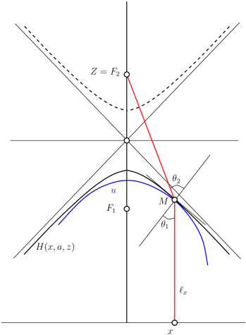
(a) Upper admissible

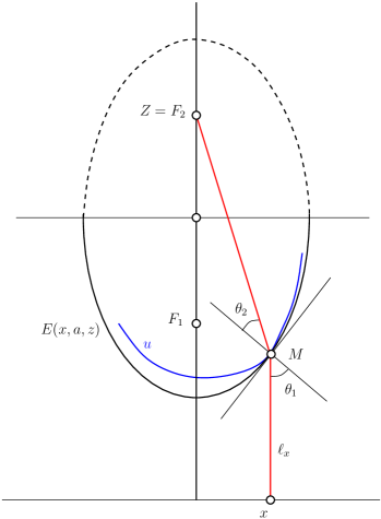
(b) Lower admissible

Figure 2. Supporting surfaces

8.1. Ellipsoids

Throughout this paper by ellipsoid we mean the lower half of an ellipsoid of revolution with focal axis parallel to $e_{n+1}$. Such surface can be regarded as the graph of

(8.1) $$E(x,a,Z)=Z^{n+1}-a\varepsilon-a\sqrt{1-\frac{(x-z)^{2}}{a^{2}(1-\varepsilon^{2})}}$$

where $a$ is the larger semiaxis, $\varepsilon$- the eccentricity, and $Z$ the higher focus, see Figure 2. Moreover we have that

(8.2) $$DE=\frac{1}{a(1-\varepsilon^{2})}\frac{x-z}{\sqrt{1-\frac{(x-z)^{2}}{a^{2}(1-\varepsilon^{2})}}}.$$

Notice that at the points $x$ where $|x-z|=a\sqrt{1-\varepsilon^{2}}$ the gradient $|DE|$ is unbounded.

8.2. Hyperboloids

It is convenient to introduce the lower sheet of hyperboloids of revolution

(8.3) $$H(x,a,Z)=Z^{n+1}-a\varepsilon-a\sqrt{1+\frac{(x-z)^{2}}{a^{2}(\varepsilon^{2}-1)}}$$

where $a$ is the larger semiaxis, $\varepsilon$ the eccentricity, and $Z$ the upper focus, see Figure 2. Differentiating $H$ we obtain

(8.4) $$DH=-\frac{1}{(\varepsilon^{2}-1)}\frac{x-z}{\sqrt{a^{2}+\frac{(x-z)^{2}}{\varepsilon^{2}-1}}}.$$

8.3. Supporting hyperboloids

Definition 8.1.

A function $u:\mathcal{U}\to\mathbb{R}$ is said to be upper (resp. lower) admissible if for any $x_{0}\in\mathcal{U}$ there is $Z\in\mathcal{V}$ and $a>0$ such that $H(x_{0},a,Z)=u(x_{0})$ (resp. $E(x_{0},a,Z)=u(x_{0})$) and $H(x,a,Z)\geq u(x),x\in\mathcal{U}$ (resp. $E(x,a,Z)=u(x)$). $H$ (resp. $E$) is called a supporting function of $u$ at $x_{0}$. The class of all upper admissible functions is denoted by $\overline{\mathbb{W}}_{\rm H}(\mathcal{U},\mathcal{V})$ (resp. $\underline{\mathbb{W}}_{\rm E}(\mathcal{U},\mathcal{V})$).

In what follows we focus on upper admissible functions, the lower admissible functions can be studied in similar fashion. If the generalisation is not straightforward then we will outline the proof.

Formula (8.4) yields uniform Lipschitz estimates for $\overline{\mathbb{W}}_{\rm H}(\mathcal{U},\mathcal{V})$.

Lemma 8.1.

Let $\mathbb{H}^{+}_{a_{0}}(\mathcal{U},\mathcal{V})$ be the set of all hyperboloids $H(x,a,Z)\geq 0,x\in\mathcal{U}$ for some $Z\in\mathcal{V}$ such that $a>a_{0}$ for some fixed $a_{0}\geq 0$. Then

(8.5) $$\sup\limits_{\mathbb{H}^{+}_{a_{0}}(\mathcal{U},\mathcal{V})}\|DH\|_{\infty}\leq\frac{1}{\sqrt{\varepsilon^{2}-1}}\frac{d_{0}}{\sqrt{a_{0}^{2}(\varepsilon^{2}-1)+d_{0}^{2}}}\quad(if\ a_{0}>0)$$

where $d_{0}=\sup_{x\in\mathcal{U},z\in\widehat{\mathcal{V}}}|x-z|.$ Furthermore,

$$\|Du\|_{L^{\infty}(\mathcal{U}^{\prime})}<\frac{1}{\sqrt{\varepsilon^{2}-1}},\quad\forall\mathcal{U}^{\prime}\subset\subset\mathcal{U},u\in{\overline{\mathbb{W}}_{\rm H}(\mathcal{U},\mathcal{V})}.$$

Proof. From (8.4) we have for $x\not=z$

$$|DH| = \frac{1}{(\varepsilon^{2}-1)}\frac{|x-z|}{\sqrt{a^{2}+\frac{|x-z|^{2}}{\varepsilon^{2}-1}}}$$

$$= \frac{1}{\sqrt{\varepsilon^{2}-1}}\frac{|x-z|}{\sqrt{a^{2}(\varepsilon^{2}-1)+|x-z|^{2}}}=\frac{1}{\sqrt{\varepsilon^{2}-1}}\frac{1}{\sqrt{\frac{a^{2}(\varepsilon^{2}-1)}{|x-z|^{2}}+1}}$$

$$\leq \frac{1}{\sqrt{\varepsilon^{2}-1}}\frac{1}{\sqrt{\frac{a^{2}(\varepsilon^{2}-1)}{\sup_{x\in\mathcal{U},z\in\widehat{\mathcal{V}}}|x-z|^{2}}+1}}.$$

If $a\geq a_{0}>0$ then the first inequality immediately follows.

In order to prove the second inequality let us suppose that for some fixed subdomain $\mathcal{U}^{\prime}\subset\subset\mathcal{U}$ there are $p_{k}\in\partial u(x_{k})$ such that $x_{k}\in\mathcal{U}^{\prime}$, $p_{k}\to p_{0},x_{k}\to x_{0}$ and $|p_{0}|=\frac{1}{\sqrt{\varepsilon^{2}-1}}$. Here $\partial u(x)$ is the subdifferential of $u$ at $x$. It is clear that $p_{0}\in\partial u(x_{0})$ and hence there is a supporting hyperplane for $u$ at $x_{0}$ with slope $p_{0}$. If $u$ is strictly concave at $x_{0}\in U$ then near $x_{0}$ one can find $\bar{x}_{0}$ such that there is $\bar{p}_{0}\in\partial u(\bar{x}_{0})$ with $|\bar{p}_{0}|>\frac{1}{\sqrt{\varepsilon^{2}-1}}$ which is in contradiction with the first inequality. Thus suppose that there is a straight segment in the graph of $u$ passing through $(x_{0},u(x_{0}))$. But this is impossible because $u$ is admissible and therefore $\Gamma_{u}$ cannot contain straight segments. ∎

Lemma 8.2.

Let $\{u_{k}\}$ be a sequence of upper admissible function such that $u_{k}\to u_{0}$ uniformly in $\mathcal{U}$. If $x_{k}\in\mathcal{U}$, $x_{k}\to x_{0}$ and $H_{k}$ are supporting functions of $u_{k}$ at $x_{k}$ then $u_{0}$ has an upper supporting function $H_{0}$ at $x_{0}$ and $H_{k}\to H_{0}$ uniformly in $\mathcal{U}$.

Proof. One way to check the claim is to use some well known fact from convex analysis. Consider the convex sets $G_{k}=\{X\in\mathbb{R}^{n+1}:x\in\mathcal{U},0<u_{k}(x)<X^{n+1}\}$ and $\mathscr{H}_{k}=\{X\in\mathbb{R}^{n+1}:x\in\mathcal{U},0<H_{k}(x)<X^{n+1}\}$ where $x=\widehat{X}$. Then $\mathscr{H}_{k}\subset G_{k}$ and $(x_{k},u_{k}(x_{k}))\in\partial\mathscr{H}_{k}\cap\partial G_{k}$. Thus, from uniform convergence $u_{k}\to u_{0}$ we infer that the limit set $G_{0}=\{X\in\mathbb{R}^{n+1}:x\in\mathcal{U},0<u_{0}(x)<X^{n+1}\}$ is a subset of $\mathscr{H}_{0}=\{X\in\mathbb{R}^{n+1}:x\in\mathcal{U},0<H_{0}(x)<X^{n+1}\}$, see [1] Chapter 5.2. Furthermore, from $x_{k}\to x_{0}\in\overline{\mathcal{U}}$ it follows that there is $X_{0}\in\partial G_{0}\cap\partial\mathscr{H}_{0}$ such that $\widehat{X}_{0}=x_{0}$. Therefore we conclude that $H_{0}$ is a supporting hyperboloid of $u_{0}$ at $x_{0}$. ∎

8.4. Continuous expansion of hyperboloids

If $u\in\overline{\mathbb{W}}_{\rm H}(\mathcal{U},\Sigma)$ then it turns out that $u$ is also admissible with respect with $\widetilde{\Sigma}$, the receiver moved vertically upwards in $e_{n+1}$ direction. In other words, the same admissible $u$ will be $R-$convex with respect to a family of surfaces obtained from $\Sigma$ by translation is $e_{n+1}$ direction. We will need this observation in order to construct smooth solutions of our problem in small balls, see Section 14.

Lemma 8.3.

Let $\widetilde{\Sigma}=\Sigma+Me_{n+1}$ for some $M>0$.

• For any fixed $x_{0}$ and $H_{1}(x)=H(x,a_{1},Z_{1})\in\mathbb{H}(\mathcal{U},\Sigma)$ there is $H_{2}(x)=H(x,a_{2},Z_{2})$ with $Z_{2}\in\widetilde{\Sigma}$ and touching $H_{1}$ from above at $x_{0}$.

• In particular if $u\in\overline{\mathbb{W}}_{\rm H}(\mathcal{U},\Sigma)$ then also $u\in\overline{\mathbb{W}}_{\rm H}(\mathcal{U},\widetilde{\Sigma})$.

Proof. (i) Let $\xi_{1}=H_{1}(x_{0})$ and $X_{0}=(x_{0},\xi_{1})$. For $s>1$ we consider $Z_{2}=X_{0}+s(Z_{1}-X_{0})$. By construction $X_{0},Z_{1}$ and $Z_{2}$ lie on the same line. To determine $a_{2}$ we utilize two geometric properties of hyperbola, namely that the difference of distances of $X_{0}$ from $Z_{2}$ and the lower focus $Z_{2}^{\prime}$ is $2a_{2}$ and $|X_{0}Z_{2}^{\prime}|=\varepsilon|X_{0}D|$ where $|X_{0}D|$ is the distance of $X_{0}$ from the lower directrix $X^{n+1}=Z^{n+1}-a_{2}\varepsilon-a_{2}/\varepsilon$. Therefore if $P$ is on the graph of $H_{2}$ we get that $|PZ_{2}|=2a_{2}+|PZ_{2}^{\prime}|=-a_{2}(\varepsilon^{2}-1)+s\varepsilon(Z_{1}^{n+1}-\xi_{1})$. Taking $P=X_{0}$ in this equation $|PZ_{2}|=\varepsilon|Z_{1}-X_{0}|$ one finds that

(8.7) $$a_{2}=\frac{1}{\varepsilon^{2}-1}[s\varepsilon(Z_{1}^{n+1}-\xi_{1})-|s(Z_{1}-X_{0})|].$$

As for (ii), we choose $s_{0}>1$ so that $X_{0}+s(Z_{1}-X_{0})\in\widetilde{\Sigma}$. Consequently from (i) it follows that $Z_{2}=X_{0}+s_{0}(Z_{1}-X_{0})$ is the focus of supporting hyperboloid $H(\cdot,a_{2},Z_{2})$ at $x_{0}$ where $a_{2}$ is given by (8.7). Therefore $u\in\overline{\mathbb{W}}_{\rm H}(\mathcal{U},\widetilde{\Sigma})$. ∎

9. $B$-type weak solutions: Proof of Theorem C1

In this section we introduce our first notion of weak solution for the refractor problem (1.6). For any upper admissible function $u\in\overline{\mathbb{W}}_{\rm H}(\mathcal{U},\mathcal{V})$ we define the mapping $\mathscr{S}_{u}:\mathcal{V}\to\mathcal{U}$ as follows

$$\mathscr{S}_{u}(Z) = \{x\in\mathcal{U}:\ \exists\ \text{a supporting hyperboloid of $u$ at $x$ with focus at $Z\in\mathcal{V}$}\}.$$

For any Borel set $\omega\subset\mathcal{V}$ we put

(9.1) $$\mathscr{S}_{u}(\omega)=\bigcup_{Z\in\omega}\mathscr{S}_{u}(Z).$$

We will write $\mathscr{S}(E)$ instead of $\mathscr{S}_{u}(E)$ if there is no confusion.

Proposition 9.1.

For $u\in\overline{\mathbb{W}}_{\rm H}(\mathcal{U},\mathcal{V})$ the corresponding mapping $\mathscr{S}$ enjoys the following properties:

• $\mathscr{S}:\mathcal{V}\longrightarrow\Pi$ maps the closed sets to closed sets.

• The mapping $\mathscr{S}$ is one-to-one modulo a set of vanishing measure, i.e.

  $$\big{|}\big{\{}x\in\Pi:x\in\mathscr{S}(Z_{1})\cap\mathscr{S}(Z_{2})\ \textrm{for}\ Z_{1}\not=Z_{2},\ \ Z_{i}\in\mathcal{V},i=1,2\big{\}}\big{|}=0.$$

• The family $\mathscr{F}=\{E\subset\mathcal{V}\ \textrm{such that}\ \mathscr{S}(E)\ \textrm{is measurable}\}$ is $\sigma-$algebra.

Proof. The first claim a) follows directly from Lemma 8.2.

In order to prove b) we set $A=\big{\{}x\in\Pi:x\in\mathscr{S}(Z_{1})\cap\mathscr{S}(Z_{2})\ \textrm{for}\ Z_{1}\not=Z_{2},\ \ Z_{i}\in\mathcal{V},i=1,2\big{\}}$. If $x\in A$ then $u$ cannot be differentiable at $x$ thanks to (2.4). Notice that if $\Sigma$ is a strictly concave graph over the plane $\{x_{n+1}=0\}$ then (2.4) is satisfied, see Remark 7.1. By Aleksandrov’s theorem the concave function $u$ is twice differentiable a.e. Hence $|A|=0$.

As for c) we must check that the following three conditions hold, see e.g. [2]

• $\mathcal{V}\in\mathscr{F}$,

• if $A\in\mathscr{F}$ then $\mathcal{V}\setminus A\in\mathscr{F}$,

• if $A_{i}\in\mathscr{F}$ then $\bigcup_{i=1}^{\infty}A_{i}\in\mathscr{F}$.

We first prove 1). If $A_{i}\in\mathcal{V}$ is any sequence of subsets of $\mathcal{V}$ then clearly $\mathscr{S}(\cup_{i=1}^{\infty}A_{i})=\cup_{i=1}^{\infty}\mathscr{S}(A_{i})$. Writing $\mathcal{V}=\cup_{i=1}^{\infty}E_{i}$, where $E_{i}\subset\mathcal{V}$ are closed subsets we conclude that $\mathscr{S}(\mathcal{V})=\mathscr{S}(\cup_{i=1}^{\infty}E_{i})=\cup_{i=1}^{\infty}\mathscr{S}(E_{i})$. From a) it follows that $\mathscr{S}(E_{i})$ is closed for any $i$, and hence measurable, implying that $\mathscr{S}(\mathcal{V})$ is measurable.

2) Let $A\in\mathscr{F}$. We use the following elementary identity

(9.2) $$\mathscr{S}(\mathcal{V}\setminus A)=[\mathscr{S}(\mathcal{V})\setminus\mathscr{S}(A)]\bigcup[\mathscr{S}(\mathcal{V}\setminus A)\cap\mathscr{S}(A)].$$

From b) it follows that $|\mathscr{S}(\mathcal{V}\setminus A)\cap\mathscr{S}(A)|=0$. Therefore $|\mathscr{S}(\mathcal{V}\setminus A)|=|\mathscr{S}(\mathcal{V})\setminus\mathscr{S}(A)|$ and 2) is proven.

It remains to check 3). Without loss of generality we assume that $A_{i}$’s are disjoint, see [2]. Thus, letting $A_{i}\in\mathscr{F},A_{i}\cap A_{j}=\emptyset,i\not=j$ we get

$$\sum_{i=1}^{\infty}|\mathscr{S}(A_{i})| \geq |\mathscr{S}(\cup_{i=1}^{\infty}A_{i})|\geq$$

$$\geq \sum_{i=1}^{\infty}|\mathscr{S}(A_{i})|-\sum_{ij=1}^{\infty}|\mathscr{S}(A_{i})\cap\mathscr{S}(A_{j})|\geq$$

$$\geq \sum_{i=1}^{\infty}|\mathscr{S}(A_{i})|.$$

∎

For a given function $u\in\mathbb{W}_{H}(\mathcal{U},\mathcal{V})$ we consider the set function

(9.3) $$\beta_{u}(\omega)=\int_{\mathscr{S}(\omega)}f$$

where $\omega\subset\mathcal{V}$ is a Borel subset. Since $\mathscr{F}$ contains the closed sets (see part a) above) we infer that $\beta_{u,f}$ is a Borel measure. Moreover, from the proof of Proposition 9.1 b) it follows that $\beta_{u,f}$ is countably additive.

Definition 9.1.

A function $u$ (or its graph $\Gamma_{u}$) is said to be a $B$-type weak solution to (1.6) if $u\in\overline{\mathbb{W}}_{\rm H}(\mathcal{U},\mathcal{V})$ and the following two identities holds

(9.6) $$\left\{\begin{array}[]{ccc}\displaystyle\beta_{u,f}(\omega)=\int_{\omega}gd\mathcal{H}^{n},\ \hbox{for\ any\ Borel\ set}\ \omega\subset\mathcal{V}\qquad\hbox{and}\\ \mathscr{S}_{u}(\mathcal{V})=\mathcal{U}.\end{array}\right.$$

9.1. Existence of weak solutions of $B$-type

The measure $\beta$, defined in (9.3) is weakly continuous. We have

Lemma 9.1.

Let $u_{k}$ be a sequence of $B$-type weak solutions in the sense of Definition 9.3 and $\beta_{k}$ is the associated measure, defined by (9.3). If $u_{k}\rightarrow u$ uniformly on compact subsets of ${\mathcal{U}}$ then $u$ is $R-$concave and $\beta_{k}$ weakly converges to $\beta_{u,f}$.

Proof. Once the $\sigma$ additivity is established then the proof of lemma is standard, see for the classical case [22] pp 14-18,[5] and [6], [11] for refractor and reflector problems respectively. The proof for supporting ellipsoids is carried out also [7]. That $u$ is admissible follows from Lemma 8.2. Recall that the weak convergence is equivalent to the following two inequalities (see [2] Theorem 4.5.1)

• $\limsup\limits_{k\rightarrow\infty}\beta_{k}(E)\leq\beta(E)$ for any compact $E\subset\mathcal{V},$

• $\liminf\limits_{k\rightarrow\infty}\beta_{k}(J)\geq\beta(J)$ for any open $J\subset\mathcal{V}$.

Take a closed set $E$ and let $E^{*}_{\delta}$ be an $\delta-$neighbourhood of the closed set $E^{*}=\mathscr{S}(E)$, see Lemma 9.1 a). We claim that for any $\delta>0$ there is $i_{0}\in\mathbb{N}$ such that $\mathscr{S}_{i}(E)\subset E^{*}_{\delta}$ whenever $i>i_{0}$, where $\mathscr{S}_{i}$ is the mapping corresponding to $u_{i}$. If this fails then there is $\delta>0$ and a sequence of points $x_{i}\in\mathscr{S}_{i}(E)$ such that $x_{i}\in\complement E_{\delta}^{*}$. By definition there is $Z_{i}\in E$ such that $x_{i}\in\mathscr{S}_{i}(Z_{i})$. Suppose that $x_{i}\rightarrow x_{0}$, for some $x_{0}$, and $Z_{i}\rightarrow Z_{0}\in E$ at least for a subsequence. Thus, $x_{0}\in\complement E^{*}_{\delta},x_{0}\in\mathscr{S}(Z_{0})$ and $Z_{0}\in E$ which is a contradiction.

To prove the second inequality we let $J\subset\mathcal{V}$ be an open subset and denote $J^{*}=\mathscr{S}(H)$. By Lemma 9.1 c) $J^{*}$ is measurable, hence for any small $\delta>0$ there is a closed set $J^{*}_{\delta}$ such that $J^{*}_{\delta}\subset J^{*}$ and $|J^{*}|-\delta\leq|J^{*}_{\delta}|\leq|J^{*}|$. This is possible because by Proposition 9.1 b) $\mathscr{S}$ is one-to-one modulo a set of measure zero. Let $N_{\delta}$ be an open set, $|N_{\delta}|<\delta$ containing the points where the inverse of $\mathscr{S}$ is not defined. We claim that there is $k_{0}$ such that

(9.7) $$J^{*}_{\delta}\setminus N_{\delta}\subset J^{*}_{k}\overset{def}{=}\mathscr{S}_{k}(J),\quad{\rm for\ any}\ k\geq k_{0}.$$

Here $\mathscr{S}_{k}$ is the mapping generated by $u_{k}$. Proof of (9.7) is by contradiction. If (9.7) fails then there is $x_{k}\in J^{*}_{\delta}\setminus N_{\delta}$ and $x_{k}\not\in J^{*}_{k}$. We can assume that $x_{k}\rightarrow x_{0}$. Since $J^{*}_{\delta}\setminus N_{\delta}$ is closed it follows that $x_{0}\in J^{*}_{\delta}\setminus N_{\delta}$. By definition of $N_{\delta}$ the inverse of $\mathscr{S}$ is one-to-one on $J^{*}_{\delta}\setminus N_{\delta}$. Thus there is a unique $Z_{0}\in H$ such that $x_{0}=\mathscr{S}(Z_{0})$. Furthermore, there is an open neighborhood of $Z_{0}$ contained in $J$ because $J$ is open. If $H(x,\sigma_{k},Z_{k})$ is a supporting hyperboloid of $u_{k}$ at $x_{k}$ it follows from Lemma 8.2 that $x_{k}\in\mathscr{S}_{k}(Z_{k}),Z_{k}\rightarrow Z_{0}$. Thus for large $k$, $\{Z_{k}\}$ is in some neighborhood of $Z_{0}\in J$ implying that $x_{k}\in J^{*}_{k}$ which contradicts our supposition.∎

Proposition 9.2.

Let $f:\mathcal{U}\to\mathbb{R}$ and $g:\mathcal{V}\to\mathbb{R}$ be two nonnegative integrable functions. If $\mathcal{U}\subset\Pi$ and $\mathcal{V}\subset\Sigma$ are bounded domains such that the energy balance condition (1.3) and (2.11) hold then there exists a $B-$type weak solution to the problem (1.6).

Notice that we do not exclude the case $\mathcal{U}\cap\widehat{\mathcal{V}}\not=\emptyset.$

Proof. The proof of Proposition 9.2 is by approximation argument, see [7], [11], [27]. Let $g_{N}=\sum_{i=1}^{N}C_{i}\delta_{Z_{i}}$ with $C_{i}\geq 0$ such that $\sum_{i=1}^{N}C_{i}=\int_{\mathcal{U}}f(x)dx,Z_{i}\in\Sigma$ and $\delta_{Z_{i}}$ are atomic measures supported at $Z_{i}$. For each $g_{N}$ we construct a $B-$type solution $u_{N}$. Then sending $N\to\infty$ and using the compactness argument together with weak convergence of $g_{N}$ to $g$, Lemma 9.1, one will arrive at desired result.

First, for each $Z\in\Sigma$ we define

(9.8) $$\bar{a}(Z)=\frac{\varepsilon Z^{n+1}-\sqrt{(Z^{n+1})^{2}+\rho^{2}}}{\varepsilon^{2}-1}$$

where

(9.9) $$\rho(z)=\inf\{R>0:\mathcal{U}\subset B_{R}(z)\}.$$

Clearly $\bar{a}(Z)$ is the maximal value of larger semiaxis of hyperboloid $H$ such that $\Gamma_{H}$ is visible from $\mathcal{U}$ in the $e_{n+1}$ direction. In other words $H(x,\bar{a}(Z),Z)$ is the lowest possible hyperboloid with focus $Z\in\Sigma$ such that $H(x,\bar{a}(Z),Z)\geq 0$. Thus for $a\in(0,\bar{a}(Z)]$ we have $H(\cdot,a,Z)\in\mathbb{H}^{+}_{0}(\mathcal{U},\mathcal{V})$. To check (9.8) we fix $Z$ and pick $x_{0}$ such that $\rho(z)=|x_{0}-z|$. Since the ratio of distances of $x_{0}$ from lower focus $Z^{\prime}$ and the plane $\Pi_{d}=\{X\in\mathbb{R}^{n+1}:X^{n+1}=Z^{n+1}-\bar{a}\varepsilon-\bar{a}/\varepsilon\}$ is $\varepsilon$, it follows that $|x_{0}Z^{\prime}|=\varepsilon(Z^{n+1}-\bar{a}\varepsilon-\bar{a}/\varepsilon)$. On the other hand $|x_{0}Z|-|x_{0}Z^{\prime}|=2\bar{a}$. Consequently, we find that $\sqrt{(Z^{n+1})^{2}+\rho^{2}(z)}=2\bar{a}+\varepsilon(Z^{n+1}-\bar{a}\varepsilon-\bar{a}/\varepsilon)$ which gives (9.8).

Next we define the maximal level $L_{0}=\sup\limits_{\mathcal{U}\times\mathcal{V}}H(x,\bar{a}(Z),Z)$. Since

$$\max_{x\in\mathcal{U}}H(x,\bar{a}(Z),Z) = Z^{n+1}-\varepsilon\bar{a}(Z)-\bar{a}(Z)=\frac{\sqrt{(Z^{n+1})^{2}+\rho^{2}(z)}-Z^{n+1}}{\varepsilon-1}$$

$$= \frac{\rho^{2}(z)}{(\varepsilon-1)(\sqrt{(Z^{n+1})^{2}+\rho^{2}(z)}+Z^{n+1})}$$

it follows that

(9.10) $$L_{0}=\sup_{\mathcal{V}}\frac{\rho^{2}(z)}{(\varepsilon-1)(\sqrt{(Z^{n+1})^{2}+\rho^{2}(z)}+Z^{n+1})}\leq\frac{1}{\varepsilon-1}\sup_{\mathcal{V}}\frac{\rho^{2}(z)}{2Z^{n+1}}.$$

Next, we bound $H(\cdot,a,Z)$ by below for $a>0$ close to zero. By definition (8.3) we have that for this case $H(x,a,Z)\sim Z^{n+1}-\frac{\rho(z)}{\sqrt{\varepsilon^{2}-1}}$. We demand $Z^{n+1}-\frac{\rho(z)}{\sqrt{\varepsilon^{2}-1}}\geq 2L_{0}$ or equivalently in lieu of (9.10)

$$Z^{n+1}\geq\rho(z)\left[\frac{1}{\sqrt{\varepsilon^{2}-1}}+\frac{2\rho(z)}{(\varepsilon-1)(\sqrt{(Z^{n+1})^{2}+\rho^{2}(z)}+Z^{n+1})}\right].$$

But clearly $\frac{2\rho(z)}{(\varepsilon-1)(\sqrt{(Z^{n+1})^{2}+\rho^{2}(z)}+Z^{n+1})}\leq 2/{(\varepsilon-1)}$. Therefore it is enough to assume that $Z^{n+1}\geq[\frac{2}{\varepsilon-1}+\frac{1}{\sqrt{\varepsilon^{2}-1}}]\rho(z)$ which is exactly (2.11). It follows that if $\Sigma$ satisfies (2.11) then $\widetilde{\Sigma}=\Sigma+Me_{n+1},M\gg 1$ also does.

Let ${\bf a}=(a_{1},\dots,a_{N}),a_{i}\in(0,\bar{a}(Z_{i})],i=1,\dots,N$ and set

$$H({\bf a},x)=\min\big{[}H(x,a_{1},Z_{1}),\dots,H(x,a_{N},Z_{N})\big{]}.$$

We also let $\cal E_{i}({\bf a})=\{x\in\mathcal{U}:H({\bf a},x)=H(x,a_{i},Z_{i})\}$ be the $i$-th visibility sets and

$$\cal A^{N}=\left\{{\bf a}\in\prod\limits_{i=1}^{N}(0,\bar{a}_{i}(Z_{i})]:\int_{\cal E_{i}({\bf a})}f\leq C_{i},\int_{\cal E_{N}({\bf a})}f\geq C_{N},\quad i=1,\dots,N-1\right\}.$$

From (2.11) it follows that $\cal A^{N}$ is not empty for taking $a_{i},1\leq i\leq N-1$ close to zero and $a_{N}=\bar{a}_{N}(Z_{N})$ one readily gets that such ${\bf a}$ is in $\cal A^{N}.$

The visibility sets $\cal E_{i}({\bf a})$ enjoy the following property: if for some $a_{k}<\bar{a}(Z_{k})$ we set ${\bf a}^{k}_{\delta}=(a_{1},\dots,a_{k}+\delta,\dots,a_{N})$ and ${\bf a}=(a_{1},\dots,a_{N})$ for $\delta>0$ small, then

(9.11) $$\cal E_{k}({\bf a})\subset\cal E_{k}({\bf a}_{\delta}^{k})\quad{\rm while}\quad\cal E_{i}({\bf a}_{\delta}^{k})\subset\cal E_{i}({\bf a}),i\not=k.$$

This can be seen for $N=2$ by simple geometric considerations, and general case is by induction.

Let $\mathfrak{a}=\sup\limits_{{\bf a}\in\cal A^{N}}\sum\limits_{i=1}^{N}a_{i}$ and $\hat{\bf a}\in\cal A^{N}$ be such that the supremum is realised, i.e. $\mathfrak{a}=\sum\limits_{i=1}^{N}\hat{a}_{i}$. We claim that $H(\hat{\bf a},x)$ solves the refractor problem with measure $g_{N}$. If not, then there is $i_{0}$, say $i_{0}=1$, such that $\int_{\cal E_{1}(\hat{\bf a})}f<C_{1}$. Then in view of the energy balance condition this implies $\int_{\cal E_{N}(\hat{\bf a})}f>C_{N}$. For $\delta>0$ small $F_{N}(\delta)=\int_{\cal E_{N}(\hat{\bf a}^{1}_{\delta})}f(x)dx\geq C_{N}$ because $F_{k}(\delta)$ is continuous function of $\delta$. Furthermore, using (9.11) it follows that ${\bf a}^{1}_{\delta}\in\cal A^{N}$ which is a contradiction. Now the proof of Theorem C1 follows from the above polyhedral approximation $H({\bf\hat{a}},x)$ as $N\to\infty$ and the weak convergence of measures $\beta_{H,f}$, Lemma 9.1. ∎

10. An approximation lemma

10.1. Refraction cone

Recall that for smooth refractors the unit direction of the refracted ray is

$$Y=\varepsilon\left(e_{n+1}+\gamma\left[\sqrt{(\gamma\cdot e_{n+1})^{2}-\kappa}-\gamma\cdot e_{n+1}\right]\right),$$

see (4.5). This formula may be generalized for non smooth refractors as follows: let $\gamma_{1},\gamma_{2}$ be the normals of two supporting planes of $u$ at $x$. Then for any two constants $c_{1},c_{2}$ the unit vector $\gamma_{c_{1}c_{2}}=\frac{c_{1}\gamma_{1}+c_{2}\gamma_{2}}{|c_{1}\gamma_{1}+c_{2}\gamma_{2}|}$ generates a mapping to the unit sphere $\mathbb{S}^{n+1}$ given by

$$\gamma_{c_{1}c_{2}}\mapsto\varepsilon\left(e_{n+1}+\gamma_{c_{1}c_{2}}\left[\sqrt{(\gamma_{c_{1}c_{2}}\cdot e_{n+1})^{2}-\kappa}-\gamma_{c_{1}c_{2}}\cdot e_{n+1}\right]\right).$$

Definition 10.1.

For $\gamma_{1},\gamma_{2}\in\mathbb{S}^{n+1}$ the refractor cone at $\xi\in\mathbb{R}^{n+1}$ is defined as

$$C_{\xi,\gamma_{1},\gamma_{2}}=\left\{Z\in\mathbb{R}^{n+1}:\frac{Z-\xi}{|Z-\xi|}=\varepsilon\left(e_{n+1}+\gamma_{c_{1}c_{2}}\left[\sqrt{(\gamma_{c_{1}c_{2}}\cdot e_{n+1})^{2}-\kappa}-\gamma_{c_{1}c_{2}}\cdot e_{n+1}\right]\right)\right\}.$$

One can easily verify that $C_{\xi,\gamma_{1},\gamma_{2}}$ is a convex cone. Indeed, for any $\gamma_{0}\perp\hbox{Span}\{\gamma_{1},\gamma_{2}\}$ we have that $\frac{Z-\xi}{|Z-\xi|}\cdot\gamma_{0}=\varepsilon(e_{n+1}\cdot\gamma_{0})$. Thus $C_{\xi,\gamma_{1},\gamma_{2}}$ is a cone.

In view of Lemma 8.1 $\|Du\|_{L^{\infty}(\mathcal{U})}\leq\frac{1}{\sqrt{\varepsilon^{2}-1}}$ for any admissible $u\in\overline{\mathbb{W}}_{\rm H}(\mathcal{U},\mathcal{V})$, and $\sqrt{(\gamma\cdot e_{n+1})^{2}-\kappa}$ is well defined thanks to this gradient estimate.

10.2. Contact set

In this subsection we study the contact set of two hyperboloids

$$\Lambda=\{x\in\mathbb{R}^{n}\ :\ H(x,a_{1},Z_{1})=H(x,a_{2},Z_{2})\}$$

where $Z_{i}\in\Sigma,a_{i}>0,i=1.2$. We show that $\Lambda$ is a conic section. To check this we simplify the equation

$$Z_{1}^{n+1}-Z_{2}^{n+1}-\varepsilon(a_{1}-a_{2})-\sqrt{a_{1}^{2}+\frac{|x-z_{1}|^{2}}{\varepsilon^{2}-1}}=-\sqrt{a_{2}^{2}+\frac{|x-z_{2}|^{2}}{\varepsilon^{2}-1}}$$

by squaring both sides of it. Then denoting $C=Z_{1}^{n+1}-Z_{2}^{n+1}-\varepsilon(a_{1}-a_{2})$ we infer

$$C^{2}-2C\sqrt{a_{1}^{2}+\frac{|x-z_{1}|^{2}}{\varepsilon^{2}-1}}+a_{1}^{2}+\frac{|x-z_{1}|^{2}}{\varepsilon^{2}-1}=a_{2}^{2}+\frac{|x-z_{2}|^{2}}{\varepsilon^{2}-1}.$$

Recognizing the terms and denoting $D=\frac{1}{2}\left[\frac{|z_{1}|^{2}-|z_{2}|^{2}}{\varepsilon^{2}-1}+C^{2}+a_{1}^{2}-a_{2}^{2}\right]$ we get

$$D+\frac{x\cdot(z_{2}-z_{1})}{\varepsilon^{2}-1}=C\sqrt{a_{1}^{2}+\frac{|x-z_{1}|^{2}}{\varepsilon^{2}-1}}.$$

By choosing a suitable coordinate system we can assume that $z_{2}-z_{1}$ is collinear to the unit direction of $x_{1}$ axis. Thus

$$D+\frac{x_{1}|z_{2}-z_{1}|}{\varepsilon^{2}-1}=C\sqrt{a_{1}^{2}+\frac{|x-z_{1}|^{2}}{\varepsilon^{2}-1}}.$$

Finally squaring both sides of the last identity and assuming that $E:=\frac{|z_{1}-z_{2}|^{2}}{\varepsilon^{2}-1}-C^{2}\not=0$ we infer

$$C^{2}\frac{|x^{\prime}-z^{\prime}_{1}|^{2}}{\varepsilon^{2}-1} = D^{2}-C^{2}a_{1}^{2}+\frac{1}{\varepsilon^{2}-1}\left(2Dx_{1}|z_{1}-z_{2}|+\frac{x_{1}^{2}|z_{1}-z_{2}|^{2}}{\varepsilon^{2}-1}-C^{2}\left[x_{1}^{2}-2x_{1}z_{1}^{1}+(z_{1}^{1})^{2}\right]\right)$$

$$= D^{2}-C^{2}a_{1}^{2}+\frac{E}{\varepsilon^{2}-1}\left(x_{1}^{2}+2x_{1}\frac{D|z_{1}-z_{2}|+C^{2}z_{1}^{1}}{E}-\frac{C^{2}(z_{1}^{1})^{2}}{E}\right)$$

$$= D^{2}-C^{2}a_{1}^{2}+\frac{E}{\varepsilon^{2}-1}\left(\left[x_{1}+\frac{D|z_{1}-z_{2}|+C^{2}z_{1}^{1}}{E}\right]^{2}-\left[\frac{D|z_{1}-z_{2}|+C^{2}z_{1}^{1}}{E}\right]^{2}-\frac{C^{2}(z_{1}^{1})^{2}}{E}\right)$$

$$= F+\frac{E}{\varepsilon^{2}-1}\left[x_{1}+\frac{D|z_{1}-z_{2}|+C^{2}z_{1}^{1}}{E}\right]^{2}$$

where

(10.1) $$E=\frac{|z_{1}-z_{2}|^{2}}{\varepsilon^{2}-1}-C^{2},\quad F=D^{2}-C^{2}a_{1}^{2}-\frac{E}{\varepsilon^{2}-1}\left(\left[\frac{D|z_{1}-z_{2}|+C^{2}z_{1}^{1}}{E}\right]^{2}+\frac{C^{2}(z_{1}^{1})^{2}}{E}\right).$$

Note that if $E=0$ then $\Lambda$ is a paraboloid. Otherwise

$$\Lambda\ \text{is}\left\{\begin{array}[]{lll}\text{the sheet of hyperboloid}\ \frac{|x^{\prime}-z_{1}^{\prime}|^{2}}{a^{2}}=F+\frac{|x_{1}-{x_{1}^{0}}|^{2}}{b^{2}}\ \text{passing through}\ x^{0},&\text{if}\ E>0,\\ \text{the ellipsoid}\ \frac{|x^{\prime}-z_{1}^{\prime}|^{2}}{A^{2}}+\frac{|x_{1}-{x_{1}^{0}}|^{2}}{B^{2}}=F\quad\text{with}\quad\frac{A^{2}}{B^{2}}=\frac{C^{2}-|z_{1}-z_{2}|^{2}}{C^{2}},&\text{if}\ E<0.\end{array}\right.$$

We see that the rotational axis of $\Lambda$ for both cases $E<0$ and $E>0$ is parallel to the direction of $z_{2}-z_{1}$. Moreover, if $\Lambda$ is an ellipsoid then this direction corresponds to the larger semiaxis. This observation will be used in the proof of Lemma 10.1 below.

10.3. R-convexity of $\mathcal{V}$

Definition 10.2.

We say that $\mathcal{V}\subset\Sigma$ is $R-$convex with respect to a point $\xi\in[0,\infty)\times\mathcal{U}$ if for any two unit vectors $\gamma_{1},\gamma_{2}$ the intersection $C_{\xi,\gamma_{1},\gamma_{2}}\cap\mathcal{V}$ is connected. If $\mathcal{V}$ is $R-$convex with respect to any $\xi\in[0,\infty)\times\mathcal{U}$ then we simply say that $\mathcal{V}$ is $R-$convex.

In particular a geodesic ball on the convex surface $\Sigma$ is an example of $R-$convex $\mathcal{V}$.

10.4. Local supporting function is also global

In the Definition 8.1 of admissibility the supporting hyperboloid $H$ is staying above $u$ in whole $\mathcal{U}$. Consequently, one may wonder if the locally admissible functions (i.e. $H$ stays above $u$ only in a vicinity of the contact point) are still in $\overline{\mathbb{W}}_{\rm H}(\mathcal{U},\mathcal{V})$. This issue was addressed by G. Loeper in [17] for the optimal transfer problems. We have

Lemma 10.1.

Under the condition (2.8) a local supporting hyperboloid is also global.

Proof. The proof is very similar to that of in [17], [25]. Let $H_{i}(x)=H(x,a_{i},Z_{i}),i=1,2$ be two global supporting hyperboloids of $u$ at $x_{0}$ such that the contact set $\Lambda\not=\{x_{0}\}$. Thus $u$ is not differentiable at $x_{0}$. To fix the ideas take $x_{0}=0$. If $\gamma_{i}$ is the normal of the graph of $H_{i},i=1,2$ at $x_{0}$ then for any $\theta\in(0,1)$ there is $Z_{\theta}\in\Sigma\cap\mathcal{C}_{0,\gamma_{1},\gamma_{2}}$ and $a_{\theta}>0$ such that $H(x)=H(x,a_{\theta},Z_{\theta})$ is a local supporting hyperboloid of $u$ at $0$ and

(10.2) $$DH_{\theta}(0)=\theta DH_{1}(0)+(1-\theta)DH_{2}(0).$$

Observe that the correspondence $\theta\mapsto Z_{\theta}$ is one-to-one thanks to the assumption (2.4), see Remark 7.1. By choosing a suitable coordinate system we can assume that $DH_{1}(0)-DH_{2}(0)=(0,\dots,0,\alpha)$ for some $\alpha>0$. Then we have that for all $0<\theta<1$

$$\min[H_{1}(x),H_{2}(x)] \leq \theta H_{1}(x)+(1-\theta)H_{2}(x)$$

$$= u(0)+\left[DH_{2}(0)+\alpha\theta\right]x_{n}+\frac{1}{2}\left[\theta D^{2}H_{1}(0)+(1-\theta)D^{2}H_{2}(0)\right]{x\otimes x}+o(|x|^{2})$$

where the last line follows from Taylor’s expansion.

Using the notations of Section 6 we have that

$$D^{2}H_{\theta}(0)=-\frac{G(x_{0},u(0),p_{1}+\theta(p_{2}-p_{1}))}{\varepsilon\kappa}$$

where we set $p_{i}=DH_{i}(0),i=1,2$ and used (10.2). For all unit vectors $\tau$ perpendicular to $x_{n}$ axis we have

$$\frac{d^{2}}{d\theta^{2}}D^{2}_{\tau\tau}H_{\theta}(0) = -\frac{d^{2}}{d\theta^{2}}\frac{G^{ij}(0,u(0),p_{1}+\theta(p_{2}-p_{1}))\tau_{i}\tau_{j}}{\varepsilon\kappa}$$

$$= -\alpha^{2}\frac{\partial^{2}}{\partial p_{n}^{2}}\frac{G^{jj}(0,u(0),p_{1}+\theta(p_{2}-p_{1}))\tau_{i}\tau_{j}}{\varepsilon\kappa}$$

$$\leq -\alpha^{2}c_{0}$$

where the last line follows from (2.8) with $c_{0}>0$, see also (6.5) and Section 7.3.

Therefore

(10.5) $$D^{2}_{\tau\tau}H_{\theta}(0)\geq\theta D^{2}_{\tau\tau}H_{1}(0)+(1-\theta)D^{2}_{\tau\tau}H_{2}(0)+\widehat{c_{0}}\theta(1-\theta)|p_{1}-p_{2}|^{2}$$

where $\widehat{c_{0}}$ depends on $c_{0}$.

Observe that at $0$ we have

(10.6) $$\theta p_{1}+(1-\theta)p_{2}=\frac{1}{\varepsilon^{2}-1}\frac{z_{\theta}}{\sqrt{a_{\theta}^{2}+\frac{|z_{\theta}|^{2}}{\varepsilon^{2}-1}}},\quad\varphi(z_{\theta})-u(0)-\varepsilon a_{\theta}=\sqrt{a_{\theta}^{2}+\frac{|z_{\theta}|^{2}}{\varepsilon^{2}-1}}$$

where we assume that $\Sigma$ is the graph of a function $\varphi$ such that $\psi(Z)=Z^{n+1}-\varphi(z)$ satisfies (2.8). From these $n+1$ equations we see that $z_{\theta}$ and $a_{\theta}$ are smooth functions of $\theta p_{1}+(1-\theta)p_{2}$. This yields the following crude estimate for the remaining second order derivatives

(10.7) $$\left|\theta D_{jn}^{2}H_{1}(0)+(1-\theta)D_{jn}^{2}H_{2}(0)-D^{2}_{jn}H(0)\right|\leq C\theta(1-\theta)|p_{1}-p_{2}|^{2},\quad j=1,\dots,n$$

where $C$ depends of $C^{2}$ form of $\varphi$. Consequently, after plugging (10.5) and (10.7) into (10.4) and recalling that $|p_{1}-p_{2}|=\alpha$ we conclude

$$\min[H_{1}(x),H_{2}(x)] \leq u(0)+\left[p_{2}+\alpha\theta\right]x_{n}+\frac{1}{2}\left[\theta D^{2}H_{1}(0)+(1-\theta)D^{2}H_{2}(0)\right]{x\otimes x}+o(|x|^{2})$$

$$= u(0)+\left[p_{2}+\alpha\theta\right]x_{n}+\frac{1}{2}D^{2}H_{\theta}(0){x\otimes x}-\widehat{c_{0}}\theta(1-\theta)\alpha^{2}\sum_{j=1}^{n-1}x_{j}^{2}+C\theta(1-\theta)\alpha^{2}|x_{n}||x|+o(|x|^{2})$$

$$= u(0)+\left[p_{2}+\alpha\theta\right]x_{n}+\frac{1}{2}D^{2}H_{\theta}(0){x\otimes x}-$$

$$-\widehat{c_{0}}\theta(1-\theta)\alpha^{2}|x|^{2}+\theta(1-\theta)\alpha^{2}(C|x_{n}||x|+\widehat{c_{0}}x_{n}^{2})+o(|x|^{2})$$

$$= u(0)+\left[p_{2}+\alpha\theta\right]x_{n}+\frac{1}{2}D^{2}H_{\theta}(0){x\otimes x}-$$

$$-\frac{\widehat{c_{0}}}{2}\theta(1-\theta)\alpha^{2}|x|^{2}+\theta(1-\theta)\alpha^{2}\left(\frac{2C^{2}}{\widehat{c_{0}}}+\widehat{c_{0}}\right)x_{n}^{2}+o(|x|^{2})$$

where the last line follows from Hölder’s inequality. Now fixing $\theta_{0}$ as in (10.2) and using the estimate $|D^{2}H_{\theta}(0)-D^{2}H_{\theta_{0}}(0)|\leq C|\theta-\theta_{0}|$ (with $C$ depending on $\varphi$) we obtain

$$\min[H_{1}(x),H_{2}(x)] \leq u(0)+\left[p_{2}+\alpha\theta_{0}\right]x_{n}+\frac{1}{2}D^{2}H_{\theta_{0}}(0){x\otimes x}+$$

$$+\alpha\left[\theta-\theta_{0}\right]x_{n}+\frac{1}{2}D^{2}H_{\theta}(0){x\otimes x}-\frac{1}{2}D^{2}H_{\theta_{0}}(0){x\otimes x}$$

$$-\frac{\widehat{c_{0}}}{2}\theta(1-\theta)\alpha^{2}|x|^{2}+\theta(1-\theta)\alpha^{2}\left(\frac{2C^{2}}{\widehat{c_{0}}}+\widehat{c_{0}}\right)x_{n}^{2}+o(|x|^{2})$$

$$\leq H_{\theta_{0}}(x)+\alpha\left[\theta-\theta_{0}\right]x_{n}+C|\theta_{0}-\theta||x|^{2}-$$

$$-\frac{\widehat{c_{0}}}{2}\theta(1-\theta)\alpha^{2}|x|^{2}+\alpha^{2}\left(\frac{2C^{2}}{\widehat{c_{0}}}+\widehat{c_{0}}\right)x_{n}^{2}+o(|x|^{2}).$$

Choosing $\theta=\theta_{0}-x_{n}\alpha\left(\frac{2C^{2}}{\widehat{c_{0}}}+\widehat{c_{0}}\right)$ such that $|x_{n}|<\delta$ with sufficiently small $\delta$ we finally obtain

$$\min[H_{1}(x),H_{2}(x)] \leq H_{\theta_{0}}(x)+C|\theta_{0}-\theta||x|^{2}-\frac{\widehat{c_{0}}}{2}\theta(1-\theta)\alpha^{2}|x|^{2}+o(|x|^{2})=$$

$$= H_{\theta_{0}}(x)-\frac{\widehat{c_{0}}}{2}\theta(1-\theta)\alpha^{2}|x|^{2}+o(|x|^{2})$$

$$\leq H_{\theta_{0}}(x),\quad\forall x\in B_{\delta}.$$

This, in particular, implies that $H_{\theta_{0}}$ is a local supporting hyperboloid near $x=0$.

It remains to check that $H_{\theta_{0}}$ is also a global supporting hyperboloid. The set $\Lambda_{1,2}=\{x\in\mathbb{R}^{n}\ :\ H_{1}(x)=H_{2}(x)\}$ passes through $0$ and splits $\mathcal{U}$ into two parts $\mathcal{U}^{+}$ and $\mathcal{U}^{-}$ (recall that $\Lambda_{12}$ is a conic section, see Section 10.2). It follows from (10.4) that the contact sets $\Lambda_{i,\theta_{0}}=\{x\in\mathbb{R}^{n}\ :\ H_{i}(x)=H_{\theta_{0}}(x)\},i=1,2$ are tangent to $\Lambda_{12}$ from one side in some vicinity of $0$, say in $\mathcal{U}^{+}$. If there is $\bar{x}_{0}\not=0$ such that, say, $\bar{x}_{0}\in\Lambda_{1,2}\cap\Lambda_{1,\theta_{0}}$ then $H_{1}(\bar{x}_{0})=H_{2}(\bar{x}_{0})=H_{\theta_{0}}(\bar{x}_{0})$ and $DH_{\theta_{0}}(\bar{x}_{0})=\bar{\theta}_{0}DH_{1}(\bar{x}_{0})+(1-\bar{\theta}_{0})DH_{2}(\bar{x}_{0})$ with possibly different $\bar{\theta}_{0}$. Observe that by construction the ray emitted from $\bar{x}_{0}$ in the direction of $e_{n+1}$ after refraction from $H_{1},H_{2}$ and $H_{\theta_{0}}$ hits the point $Z_{1},Z_{2}$ and $Z_{\theta_{0}}$, respectively. Then repeating the argument above with $0$ replaced by $\bar{x}_{0}$ and $\theta_{0}$ by $\bar{\theta}_{0}$ (but keeping $H_{\theta_{0}}$ fixed), we can see that (10.4) is satisfied in $B_{\delta}(\bar{x}_{0})$ implying that $\Lambda_{1,\theta_{0}}$ is tangent with $\Lambda_{1,2}$ at $\bar{x}_{0}$ and lies in $\mathcal{U}^{+}$. Thus $H_{\theta_{0}}$ is a global supporting hyperboloid. ∎

As an application of Lemma 10.1 we have the following approximation result.

Lemma 10.2.

If $u\in\overline{\mathbb{W}}_{\rm H}(B_{r},\Sigma)$ then

• $u_{\varepsilon}(x)+K(r^{2}-|x|^{2})\in\overline{\mathbb{W}}_{\rm H}(B_{r},\widetilde{\Sigma})$ where $u_{\varepsilon}$ is the standard mollification of $u$, $K>0$ and $\widetilde{\Sigma}=\Sigma+Me_{n+1}$ for some large constant $M>0$,

• $u_{\varepsilon}(x)+K(r^{2}-|x|^{2})$ is a classical subsolution of (6.2).

Proof. (i) It is well known that $u_{\varepsilon}$ is concave and $\|Du_{\varepsilon}\|_{L^{\infty}(B_{r})}\leq\|Du\|_{L^{\infty}(B_{r})}<\frac{1}{\sqrt{\varepsilon^{2}-1}}$. Therefore if $K$ is fixed then we can choose $r$ so small that

(10.9) $$\|D\bar{u}_{\varepsilon}\|_{L^{\infty}(B_{r})}\leq\|Du\|_{L^{\infty}(B_{r})}+2Kr<\frac{1}{\sqrt{\varepsilon^{2}-1}}.$$

Moreover $K(r^{2}-|x|^{2})$ is concave, hence $\bar{u}_{\varepsilon}=u_{\varepsilon}(x)+K(r^{2}-|x|^{2})$ is concave as well. Notice that $D^{2}\bar{u}_{\varepsilon}=D^{2}u_{\varepsilon}-2K{\rm{Id}}\leq-2K{\rm{Id}}<0$ implying that $\bar{u}_{\varepsilon}$ is strictly concave. In order to bound the curvature of $\Gamma_{\bar{u}_{\varepsilon}}$ from below we recall that for fixed $Z$, $H(\cdot,a,Z)$ becomes flatter as $a\to\infty$ because

$$D^{2}H=-\frac{1}{(\varepsilon^{2}-1)\sqrt{a^{2}+\frac{|x-z|^{2}}{\varepsilon^{2}-1}}}\left[{\rm{Id}}-\frac{(x-z)\otimes(x-z)}{(\varepsilon^{2}-1)a^{2}+|x-z|^{2}}\right].$$

In particular, for large $K$ and $a$ we will have $-D^{2}\bar{u}_{\varepsilon}\geq 2K{\rm{Id}}\geq-D^{2}H$. Consequently, for each $x\in\mathcal{U}$ there is $Z$ and $a>0$ such that $H(\cdot,a,Z)$ touches $\bar{u}_{\varepsilon}$ from above at $x$, in some neighbourhood of $x$. Furthermore, from Lemma 8.3 on confocal expansion we can choose $a,\widetilde{Z}$ so that $\widetilde{Z}\in\widetilde{\Sigma}=\Sigma+Me_{n+1},M\gg 1.$ Finally applying Lemma 10.1 we infer that $H(\cdot,a,\widetilde{Z})$ is a global supporting hyperboloid of $u$ at $x$ and thus $\bar{u}_{\varepsilon}\in\overline{\mathbb{W}}_{\rm H}(\mathcal{U},\widetilde{\Sigma})$.

(ii) By direct computation we have

$$\cal M = -D^{2}\bar{u}_{\varepsilon}-\frac{G(x,\bar{u}_{\varepsilon},D\bar{u}_{\varepsilon})}{\varepsilon\kappa}=-D^{2}u_{\varepsilon}+2K{\rm{Id}}-\frac{G(x,\bar{u}_{\varepsilon},D\bar{u}_{\varepsilon})}{\varepsilon\kappa}\geq$$

$$\geq 2K{\rm{Id}}-\frac{G(x,\bar{u}_{\varepsilon},D\bar{u}_{\varepsilon})}{\varepsilon\kappa}.$$

By definition, (6.1) we have

$$\frac{G(x,\bar{u}_{\varepsilon},D\bar{u}_{\varepsilon})}{\varepsilon\kappa}=\frac{[q+1]({\rm{Id}}-\varepsilon^{2}\kappa D\bar{u}_{\varepsilon}\otimes D\bar{u}_{\varepsilon})}{\varepsilon\kappa t(x,\bar{u}_{\varepsilon},D\bar{u}_{\varepsilon})}\leq\frac{C}{t(x,\bar{u}_{\varepsilon},D\bar{u}_{\varepsilon})}$$

with some tame constant $C>0$ depending only on $\varepsilon$. Recall that by (2.10) $t=\frac{(M+[Z^{n+1}-\bar{u}_{\varepsilon}])}{Y^{n+1}}\sim\frac{M}{c(\varepsilon)},Z\in\Sigma$. Therefore choosing $M$ large enough, one sees that $\cal M\geq\left[2K-\frac{Cc(\varepsilon)}{M}\right]{\rm{Id}}\geq K{\rm{Id}}$ if $K>\frac{Cc(\varepsilon)}{M}$. Fixing $K\geq\max\left[\frac{Cc(\varepsilon)}{M},\sup|h|^{\frac{1}{n}}\right]$, where $h$ is defined by (6.4) and choosing $r$ small enough such that (10.9) holds we finally arrive at $\text{det}\left[-D^{2}\bar{u}_{\varepsilon}-\frac{G(x,\bar{u}_{\varepsilon},D\bar{u}_{\varepsilon})}{\varepsilon\kappa}\right]\geq|h|$ and the proof is complete. ∎

11. $A$-type weak solutions and the Legendre-like transform

In this section we are concerned with the second notion of weak solution to (1.6). For $u\in\overline{\mathbb{W}}_{\rm H}(\mathcal{U},\mathcal{V})$ let us consider the mapping $\mathscr{R}_{u}:\mathcal{U}\to\Sigma$ defined as

$$\mathscr{R}_{u}(x)=\{Z\in\Sigma:\mbox{there \ is\ a \ supporting \ hyperboloid}\ H(\cdot,a,Z)\ \mbox{ of}\ u\ \mbox{at}\ x\}.$$

Let $E\subset\mathcal{U}$ be a Borel set and put

$$\mathscr{R}_{u}(E)=\bigcup_{x\in E}\mathscr{R}_{u}(x).$$

Our primary goal is to prove that $\mathscr{R}_{u}(E)$ is measurable with respect to the restriction of $\mathcal{H}^{n}$ on $\Sigma$ for any Borel set $E\subset\mathcal{U}$. That done, we can proceed as in [11] and establish that the set function $\alpha_{u,g}$ is $\sigma$-additive measure.

To take advantage of the geometric intuition coming from supporting hyperboloids of $u\in\overline{\mathbb{W}}_{\rm H}(\mathcal{U},\mathcal{V})$ it is convenient to define the Legendre-like transformation of $u$. We use the construction of smallest focal parameter introduced by Xu-Jia Wang in [27] (equation (1.15)). Let $u\in\overline{\mathbb{W}}_{\rm H}(\mathcal{U},\Sigma)$ and $Z\in\Sigma$ be a fixed point. Then the smallest semi-axis among all hyperboloids $H(\cdot,a,Z)$ that stay above $u$ is

$$a_{0}=\sup_{a\in I(Z)}a,\quad I(Z)=\{a>0:H(x,a,Z)\geq u(x)\ \mbox{in }\ \mathcal{U}\}.$$

Suppose that $H(\cdot,a_{0},Z)$ touches $u$ at $x_{0}\in\mathcal{U}$ then

$$u(x_{0})=\psi(z)-a_{0}\varepsilon-\sqrt{a^{2}_{0}+\frac{(x_{0}-z)^{2}}{\varepsilon^{2}-1}}.$$

From here we can easily find that

(11.1) $$a_{0}=\frac{1}{\varepsilon^{2}-1}\left\{\varepsilon[u(x_{0})-\psi(z)]-\sqrt{[u(x_{0})-\psi(z)]^{2}+(x_{0}-z)^{2}}\right\}.$$

Alternatively, one can use the property that the distance of a point $P$ on hyperboloid from lower focus $Z^{\prime}$ is $\varepsilon$ times the distance of $P$ from the hyperplane $\Pi_{d}=\{X\in\mathbb{R}^{n+1}:X^{n+1}=Z^{n+1}-a\varepsilon-\frac{a}{\varepsilon}\}$ (which in one dimensional case is the directrix). Since by definition of hyperboloid $|PZ|-|PZ^{\prime}|=2a$ and $|PZ^{\prime}|=\varepsilon\text{dist}(P,\Pi_{d})$ we infer $|PZ|=2a+\varepsilon([\psi(z)-u(x_{0})]-a\varepsilon-\frac{a}{\varepsilon})=-a(\varepsilon^{2}-1)+\varepsilon([\psi(z)-u(x_{0})]$ and (11.1) follows.

11.1. $A$-type weak solutions

Definition 11.1.

Let $u\in\overline{\mathbb{W}}_{\rm H}(\mathcal{U},\Sigma)$ then

(11.2) $$v(z)=\inf_{x\in\mathcal{U}}\left\{\varepsilon[\psi(z)-u(x)]-\sqrt{[u(x)-\psi(z)]^{2}+(x-z)^{2}}\right\}$$

is called the Legendre-like transformation of $u$.

If $\text{dist}(\mathcal{U},\mathcal{V})>0$ and $\psi\in C^{2}$ then the function $\mathscr{L}_{x}(z)=\varepsilon[\psi(z)-u(x)]-\sqrt{[u(x)-\psi(z)]^{2}+(x-z)^{2}}$ is $C^{2}$-smooth for any fixed $x\in\mathcal{U}$. Since $v$ is the upper envelope of $C^{2}$ smooth functions $\mathscr{L}_{x},x\in\mathcal{U}$ ($x$ being the parameter) then $v(z)$ is semi-convex. Next lemma gives an important characterization of $v(z)$.

Lemma 11.1.

Let $v$ be the Legendre-like transformation of $u\in\overline{\mathbb{W}}_{\rm H}(\mathcal{U},\Sigma)$. Then

• $v(z)=\varepsilon[\psi(z)-u(x_{0})]-\delta_{u}(x_{0},z)$ if $Z=(z,\psi(z))\in\mathscr{R}_{u}(x_{0})$ where $\delta_{u}(x,z)=\sqrt{[u(x)-\psi(z)]^{2}+(x-z)^{2}}$,

• $v(z)$ is semi-concave.

Proof. By definition $v(z)$ is locally bounded, non-negative, lower semi-continuous function. Let $\delta_{u}(x,z)$ denote the distance between the points of graph $\Gamma_{u}$ and $\Sigma$. To check (i) we first observe that by definition of $v(z)$, see (11.2), we have $v(z)\leq\varepsilon[\psi(z)-u(x_{0})]-\delta_{u}(x_{0},z)$. If $v(z)<\varepsilon[\psi(z)-u(x_{0})]-\delta_{u}(x_{0},z)$ it follows from (11.1) and the discussion above that $H(\cdot,a_{0},Z)$ is a supporting hyperboloid of $u$ at $x_{0}$, where $a_{0}=(\varepsilon^{2}-1)^{-1}(\varepsilon[\psi(z)-u(x_{0})]-\delta_{u}(x_{0},z))$ because $Z\in\mathscr{R}_{u}(x_{0})\subset\Sigma$. On the other hand, there is a sequence $\{x_{k}\}$ in $\mathcal{U}$ such that $x_{k}\to\bar{x}_{0}\in\overline{\mathcal{U}}$ and $\lim\limits_{x_{k}\to\bar{x}_{0}}\left(\varepsilon[\psi(z)-u(x_{k})]-\delta_{u}(x_{k},z)\right)=v(z)$. Setting $\bar{a}_{0}=(\varepsilon^{2}-1)^{-1}v(z)$ we conclude that $H(\cdot,\bar{a}_{0},Z)$ is touching $\Gamma_{u}$ at $\bar{x}_{0}$. By construction $\bar{a}_{0}<a_{0}$ and it follows from confocal expansion of hyperboloids 8.4 that $H(\cdot,\bar{a}_{0},Z)>H(\cdot,a_{0},Z)$ in $\mathcal{U}$. But this inequality is in contradiction with the fact that $H(\cdot,a_{0},Z)$ is a supporting hyperboloid of $u$ at $x_{0}$ and $H(\cdot,\bar{a}_{0},Z)$ touches $\Gamma_{u}$ at $\bar{x}_{0}$ whilst staying above $\Gamma_{u}$.

To prove (ii) we let $\mathscr{L}_{x_{0}}(y)=\varepsilon[\psi(z)-u(x_{0})]-\delta_{u}(x_{0},y)$. Then

$$v(y)=\inf\limits_{x\in\mathcal{U}}\big{\{}\varepsilon[\psi(z)-u(x)]-\delta_{u}(x,y)\big{\}}\leq\varepsilon[\psi(z)-u(x_{0})]-\delta_{u}(x_{0},y)$$

which implies that $v(y)\leq\mathscr{L}_{x_{0}}(y)$ and $v(z)=\mathscr{L}_{x_{0}}(z)$, where $Z\in\mathscr{R}_{u}(x_{0})$. We can regard $\mathscr{L}_{x_{0}}(y)$ as an upper supporting function of $v$ at $z$. Differentiating $\mathscr{L}_{x_{0}}$ twice in $z$ variable we see that $|D^{2}\mathscr{L}_{x_{0}}(z)|\leq\frac{C}{(\text{dist}(\mathcal{U},\mathcal{V}))^{3}}$ for some tame constant $C>0$, consequently $v(z)-C|z|^{2}$ is concave for large $C>0$. ∎

The main result of this section is contained in the following

Lemma 11.2.

Let $\cal S=\{Z\in\mathcal{V}:\mbox{such \ that}\ Z\in\mathscr{R}_{u}(x_{1})\cap\mathscr{R}_{u}(x_{2}),x_{1}\neq x_{2}\}$. Then $\cal S$ has vanishing surface measure on $\Sigma$.

Proof. Let us show that if $Z\in\cal S$ then the Legendre-like transformation of $u$ is not differentiable at $Z$. This will suffice to conclude the proof because by definition $v$ is semiconcave and hence by Aleksandrov’s theorem twice differentiable almost everywhere. Let $v$ be the Legendre-like transformation of $u$, then by Lemma 11.1 for any $Z\in\mathscr{R}_{u}(x_{0})$ at which $v(z)$ is differentiable there holds

(11.3) $$Dv(z)=\varepsilon D\psi(z)-(y(x)+D\psi(z)y^{n+1}(x)).$$

Indeed, $Dv(z)=\varepsilon D\psi(z)-{\delta_{u}(x,z)}^{-1}\left[(z-x)+D\psi(z)(\psi(z)-u(x))\right]$. From the definition of stretch function $t$ it follows that $(z-x,\psi(z)-u(x))=Y\delta_{u}(x,z)$ where $Y=(y,y^{n+1})$ is the unit direction of the refracted ray and (11.3) follows. Consequently, if $x_{1}\neq x_{2}$ such that $\mathscr{R}_{u}(x_{1})\cap\mathscr{R}_{u}(x_{2})\ni Z$ then we must have

$$Dv(z)=-\frac{z-x_{i}+D\psi(z)(\psi(z)-x_{i})}{\delta_{u}(x_{i},z)}+\varepsilon D\psi(z),\quad i=1,2.$$

Equating the right hand sides for $i=1$ and $i=2$ we obtain

$$\frac{z-x_{1}+D\psi(z)(\psi(z)-x_{1})}{\delta_{u}(x_{1},z)}=\frac{z-x_{2}+D\psi(z)(\psi(z)-x_{2})}{\delta_{u}(x_{2},z)}$$

With the aid of this observation and (11.3) we can rewrite the last line as follows

$$y_{1}+D\psi(z)y^{n+1}_{1}=y_{2}+D\psi(z)y_{2}^{n+1}\ {\rm in}\ \mathbb{R}^{n}\quad\Rightarrow\quad Y_{1}+(D\psi(z),-1)y_{1}^{n+1}=Y_{2}+(D\psi(z),-1)y_{2}^{n+1},\ {\rm in}\ \mathbb{R}^{n+1}.$$

The last identity implies that $Y_{1}-Y_{2}$ is collinear to the normal of $\Sigma$ at $Z$. Consequently, from the assumption (2.4) (see also (2.10)) we obtain that this is possible if and only if $Y_{1}=Y_{2}$. Next, from $Y_{1}=Y_{2}$ we have $y_{1}=y_{2}$ and consequently we conclude that

(11.4) $$\frac{z-x_{1}}{\delta_{u}(x_{1},z)}=\frac{z-x_{2}}{\delta_{u}(x_{2},z)}.$$

Taking the reciprocal of both sides in the last identity and recalling the definition of the distance $\delta_{u}(x,z)$ one gets

$$\frac{u(x_{1})-\psi(z)}{|x_{1}-z|} = \frac{u(x_{2})-\psi(z)}{|x_{2}-z|}$$

yielding

$$u(x_{1}) = \psi(z)+\frac{|z-x_{1}|}{|z-x_{2}|}(u(x_{2})-\psi(z))$$

$$= \psi(z)+\frac{\delta_{u}(x_{1},z)}{\delta_{u}(x_{2},z)}(u(x_{2})-\psi(z)).$$

On the other hand $Y^{n+1}_{1}=Y^{n+1}_{2}$ gives $u(x_{1})-u(x_{2})=\delta_{u}(x_{2},z)-\delta_{u}(x_{1},z)$ and hence combining this with the last equation yields

$$\psi(z)\left[1-\frac{\delta_{u}(x_{1},z)}{\delta_{u}(x_{2},z)}\right]-u(x_{2})\left[1-\frac{\delta_{u}(x_{1},z)}{\delta_{u}(x_{2},z)}\right]=\delta_{u}(x_{1},z)-\delta_{u}(x_{2},z).$$

If $\delta_{u}(x_{2},z)\not=\delta_{u}(x_{1},z)$ then the last equality implies $u(x_{2})-\psi(z)=\sqrt{(u(x_{2})-\psi(z))^{2}+(z-x_{2})^{2}}$. Hence $x_{2}=z$ and by (11.4) $x_{1}=x_{2}$, which is contradiction. Thus we must have $\delta_{u}(x_{2},z)=\delta_{u}(x_{1},z)$ and in view of (11.4) this implies that $x_{1}=x_{2}$, again contradicting our supposition. Therefore we infer that $v(z)$ cannot be differentiable at $z$. By Rademacher’s theorem $v(z)$ is differentiable a.e. in $z$. Thus $\cal S$ has vanishing surface measure. ∎

Corollary 11.1.

For any $u\in\overline{\mathbb{W}}_{\rm H}(\mathcal{U},\mathcal{V})$ and any Borel subset $E\subset\mathcal{U}$ the set function

(11.5) $$\alpha_{u,g}(E)=\int_{\mathscr{R}_{u}(E)}gd\mathcal{H}^{n}$$

is a Radon measure.

Proof. In order to show that $\alpha_{u,g}$ is Radon measure it suffices to check that $\widetilde{\mathscr{F}}=\{E\subset\mathcal{U}:\mathscr{R}_{u}(E)\ \mbox{is measurable}\}$ is a $\sigma-$algebra. This can be done exactly in the same way as in the proof of Proposition 9.1 c). It remains to recall that by Lemma 8.2, $\widetilde{\mathscr{F}}$ contains the closed sets. ∎

Definition 11.2.

A function $u\in\overline{\mathbb{W}}_{\rm H}({\mathcal{U},\mathcal{V}})$ is said to be $A$-type weak solution of (1.6) if $\int_{E}f(x)dx=\alpha_{u,g}(E)$ or any Borel set $E\subset\mathcal{U}$ and

(11.6) $$\overline{\mathcal{V}}\subset\overline{\mathscr{R}_{u}(\mathcal{U})},\qquad|\{x\in\mathcal{U}:\mathscr{R}_{u}(x)\not\subset\mathcal{V}\}|=0$$

This definition is natural, stating that the target domain $\mathcal{V}$ is covered by the refracted rays and the endpoints of those rays that after refraction do not strike $\mathcal{V}$ constitute a null set on $\mathcal{U}$. We shall establish the existence of $A$-type weak solution in the next section.

In closing this section we state the weak convergence result for the $\alpha$-measures, see Corollary 11.1.

Lemma 11.3.

Let $u_{k}$ be a sequence of $A$-type weak solutions and $\alpha_{k}$ is the corresponding measure, defined by (11.5). If $u_{k}\rightarrow u$ uniformly on compact subsets of ${\mathcal{U}}$ then $u$ is $R-$concave and $\alpha_{k}$ weakly converges to $\alpha_{u,g}$.

The proof is very similar to that of Lemma 9.1 (modulo minor adjustments) and hence omitted.

Remark 11.1.

The Legendre like transformation (11.2) can be used to reformulate (1.6) as a nonlinear optimization problem, following the method set out in [15].

12. Comparing $A$ and $B$ type weak solutions: Proof of Theorem C3-4

In this section we prove the equivalence of $A$ and $B$ type weak solutions under some conditions. These results are known for in $\mathbb{R}^{n}$ for the sub-differential [4], [26]. Let $\varphi:\mathbb{R}^{N}\to\mathbb{R}^{n}$ be a Borel mapping and $\mu(\mathbb{R}^{N})=\nu(\mathbb{R}^{n})<\infty$ with $\mu,\nu$ being two Radon measure on $\mathbb{R}^{N}$ and $\mathbb{R}^{n}$, respectively. Then $\varphi$ induces a (push-forward) measure on $\mathbb{R}^{n}$ defined by $\varphi_{\#}\mu(E)=\mu(\varphi^{-1}(E))$ for Borel subsets $E\subset\mathbb{R}^{n}$. We say that a Borel mapping $\varphi$ measure preserving if

(12.1) $$\varphi_{\#}\mu(E)=\nu(E)\qquad\mbox{for any Borel set}\ E\subset\mathbb{R}^{n}.$$

By the change of variables formula (12.1) can be rewritten in the following equivalent form

(12.2) $$\int h(\varphi(x))d\mu=\int h(y)d\nu,\qquad\forall h\in C(\mathbb{R}^{n}),$$

see [3].

Remark 12.1.

If $u\in\mathbb{W}^{+}(\mathcal{U},\Sigma)$ is the $B$-type solution of (1.6), the existence of which is established in Section 9, then taking $\varphi(Z)=\mathscr{S}_{u}(Z),N=n+1$, $d\mu=gd\mathcal{H}^{n}$, and $\nu$ being the Lebesgue measure one immediately observes that $\mathscr{S}_{u}$ is measure preserving in the sense of (12.1) or (12.2).

Lemma 12.1.

If $\mathscr{R}_{u}(x)\subset\mathcal{V}$ for a.e. $x\in\mathcal{U}$ then $\mathscr{R}_{u}(E)\subset\mbox{\rm Hull}(\mathcal{V})$, where $\mbox{\rm Hull}(\mathcal{V})$ is the R-convex hull of $\mathcal{V}$ defined as the smallest R-convex subset of $\Sigma$ containing $\mathcal{V}$.

Proof. We only have to consider the points where $u$ is non-differentiable. Let $u$ be non-differentiable at $x_{0}\in\mathcal{U}$ and suppose that $\gamma_{1},\gamma_{2}$ are the normals of two supporting planes of $u$ at $x_{0}$. The ray with endpoint $x_{0}$ after reflection will lie in the reflector cone $\cal C_{\xi_{0},\gamma_{1},\gamma_{2}}$, with $\xi_{0}=(x_{0},u(x_{0}))$ and the reflected ray will strike $\mbox{Hull}(\mathcal{V})$, because $\cal C_{\xi_{0},\gamma_{1},\gamma_{2}}\cap\mbox{Hull}(\mathcal{V})$ is connected. Considering all normals of supporting planes at $x_{0}$ we obtain the desired result. ∎

Proposition 12.1.

Let $\Sigma$ be $R-$convex with respect to $Q_{m}=\mathcal{U}\times(0,m),m>0$ and the densities $f,g$ are positive. Then $B$-type weak solution is also of $A$-type.

Proof. We split the proof into three parts.

1) First we show that for any compact $K_{1}\subset\mathcal{U}$ there holds $\int_{K_{2}}gd\mathcal{H}^{n}\geq\int_{K_{1}}f(x)dx$ with $K_{2}=\mathscr{R}_{u}(K_{1})$. In other words the $B$-type solution is $A$-type subsolution. It is worthwhile to point out that for the proof of this inequality we don’t need $\mathcal{V}$ to be $R-$convex. Take $\eta\in C(\Sigma)$ such that $\eta\equiv 1$ on $K_{2}\subset\Sigma$ and $0\leq\eta\leq 1$. From (12.2) we see that

$$\int_{\mathcal{V}}\eta gd\mathcal{H}^{n}=\int_{\mathcal{U}}\eta(\mathscr{R}_{u}(x))f(x)dx\geq\int_{K_{1}}f(x)dx.$$

Letting $\eta$ to decrease to the characteristic function of $K_{2}$, $h\downarrow\chi_{K_{2}}$ we infer

(12.3) $$\int_{K_{2}}gd\mathcal{H}^{n}\geq\int_{K_{1}}f(x)dx.$$

Notice by Corollary 11.1 the measure $\alpha_{u,g}$ is Borel regular, therefore in the last inequality $K_{1}$ can be replaced by any Borel subset of $\mathcal{U}$. As a result we conclude from (12.3) that

(12.4) $$\mbox{if}\ \mathcal{H}^{n}(\mathscr{R}_{u}(E))=0\ \mbox{then}\ |E|=0.$$

2) Next, we prove the converse estimate of (12.3). Here we will utilize the $R-$convexity of $\mathcal{V}$. Take any compact $K_{1}\in\mathcal{U}$ and apply Lemma 11.2 to conclude $\mathcal{H}^{n}\big{(}\mathscr{R}_{u}(K_{1})\cap\mathscr{R}_{u}(\mathcal{U}\setminus K_{1})\big{)}=0$. Let us show that

(12.5) $$|\mathscr{R}_{u}^{-1}(\mathscr{R}_{u}(K_{1}))\setminus K_{1}|=0$$

where $\mathscr{R}_{u}^{-1}(\mathscr{R}_{u}(K_{1}))$ is the pre-image of $\mathscr{R}_{u}(K_{1})$. Denote $E=\mathscr{R}_{u}^{-1}(\mathscr{R}_{u}(K_{1}))$ and $G=K_{1}$. If $\mathcal{H}^{n}(E\setminus G)=0$ then in view of (12.4) we obtain (12.5). Indeed, form the identity (9.2) it follows that

$$|\mathscr{R}_{u}(E\setminus G)| = \left|[\mathscr{R}_{u}(E)\setminus\mathscr{R}_{u}(G)]\bigcup[\mathscr{R}_{u}(E\setminus G)\cap\mathscr{R}_{u}(G)]\right|$$

$$= |\mathscr{R}_{u}(E\setminus G)\cap\mathscr{R}_{u}(G)|$$

$$= 0$$

where to get the last line we used the definitions of $E$ and $G$ in order to obtain $\mathscr{R}_{u}(E)\setminus\mathscr{R}_{u}(G)=\mathscr{R}_{u}(K_{1})\setminus\mathscr{R}_{u}(K_{1})=\emptyset$ and Lemma 11.2. Thus (12.4) implies $0=|E\setminus G|=|\mathscr{R}_{u}^{-1}(\mathscr{R}_{u}(K_{1}))\setminus K_{1}|$.

Let $h\in C(\Sigma)$ such that $0\leq h\leq 1$ and $h\geq\chi_{\mathscr{R}_{u}(K_{1})}$. Since $\mathcal{V}$ is $R-$convex it follows that $\mathscr{R}_{u}(K_{1})\subset\hbox{Hull}\mathcal{V}$, see Lemma 12.1. If $u$ is a $B$-type weak solution then (12.2) holds, see Remark 12.1. Therefore

$$\int_{\mathcal{U}}\eta(\mathscr{R}_{u}(x))f(x)dx = \int_{\mathcal{V}}\eta gd\mathcal{H}^{n}$$

$$= \int_{\textrm{Hull}(\mathcal{V})}\eta gd\mathcal{H}^{n}$$

$$\geq \int_{\mathscr{R}_{u}(K_{1})}gd\mathcal{H}^{n}.$$

Letting $\eta\rightarrow 0$ on compact subsets of $\mathcal{V}\setminus\mathscr{R}_{u}(K_{1})$, it follows that $\eta(\mathscr{R}_{u}(x))$ uniformly converges to zero one the compact subsets of $\mathcal{U}\setminus\mathscr{R}_{u}^{-1}(\mathscr{R}_{u}(K_{1}))$. Consequently

$$\int_{\mathscr{R}_{u}(K_{1})}gd\mathcal{H}^{n}\leq\int_{\mathcal{U}}\eta(\mathscr{R}_{u}(x))f(x)dx\longrightarrow\int_{\mathscr{R}^{-1}(\mathscr{R}_{u}(K_{1}))}f(x)dx=\int_{K_{1}}f(x)dx$$

where the last line follows from (12.5). This implies that $u$ is a supersolution.

3) It remains to check that $u$ verifies the boundary condition (11.6). Suppose that there is $Z_{0}\in\overline{\mathcal{V}}$ such that $Z_{0}\not\in\overline{\mathscr{R}_{u}(\mathcal{U})}$. Since $u$ is of $B$-type, it follows that $\mathscr{S}_{u}(\mathcal{V})=\mathcal{U}$ implying $x_{0}\in\mathscr{S}_{u}(Z_{0})$ in other words, there is a supporting hyperboloid $H(x,a_{0},Z_{0})$ at $x_{0}$. Thus $Z_{0}\in\mathscr{R}_{u}(x_{0})$which yields $\overline{\mathcal{V}}\subset\overline{\mathscr{R}_{u}(\mathcal{U})}$. From energy balance condition we have

$$\int_{\overline{\mathscr{R}_{u}(\mathcal{U})}}gd\mathcal{H}^{n}=\int_{\mathcal{U}}f(x)dx=\int_{\mathcal{V}}gd\mathcal{H}^{n}\quad\Rightarrow\quad\int_{\overline{\mathscr{R}_{u}(\mathcal{U})}\setminus\mathcal{V}}g=0.$$

This yields $|\{x\in\mathcal{U}:\mathscr{R}_{u}(x)\not\subset\mathcal{V}\}|=0$ for $f,g>0$. ∎

Remark 12.2.

We always have $\overline{\mathcal{V}}\subset\mathscr{R}_{u}(\mathcal{U})$, however if in addition $\Sigma$ is $R-$convex then it follows that $\mathscr{R}_{u}(\mathcal{U})\subset\mathcal{V}$. Thus we get the equality $\overline{\mathscr{R}_{u}(\mathcal{U})}=\overline{\mathcal{V}}$ for R-convex $\mathcal{V}$.

12.1. Existence of $A$-type weak solutions: Proof of Theorem C4

Suppose that $\mathcal{V}\subset\Sigma$ and let $\mbox{\rm Hull}(\mathcal{V})$ be the $R-$convex hull of $\mathcal{V}$. For small $\delta,\delta^{\prime}>0$ we consider

(12.7) $$g_{\delta}(Z)=\left\{\begin{array}[]{lll}g(Z)-\delta&\mbox{if}\ Z\in\mathcal{V}\\ \delta^{\prime}&\mbox{if}\ Z\in\mbox{Hull}(\mathcal{V})\setminus\mathcal{V}\end{array}\right.$$

where we choose $\delta,\delta^{\prime}$ so that $g_{\delta}$ satisfies the energy balance condition (1.3). By Proposition 9.2 for each $g_{\delta}$ there is a $B$-type weak solution which according to Proposition 12.1 is also of $A$-type. Moreover, from Remark 12.2 we infer

(12.8) $$\overline{\mathscr{R}_{u_{\delta}}(\mathcal{U})}=\overline{\mathcal{V}}.$$

Sending $\delta\rightarrow 0$ we obtain from Lemma 11.3 that $u_{\delta}\rightarrow u$ and $u$ is an $A$-type solution, i.e. (11.5) is satisfied, and

(12.9) $$\overline{\mathcal{V}}\subset\overline{\mathscr{R}_{u}(\mathcal{U})}.$$

Since $u$ is second order differentiable a.e. in $\mathcal{U}$ it follows that $\mathscr{R}_{u}$ is defined for a.e. $x\in\mathcal{U}$. Finally we want to show that $|S|=0$ where $S=\{x\in\mathcal{U}:\exists Z\in\mathscr{R}_{u}(x)\ \mbox{such\ that}\ Z\in\mathscr{R}_{u}(\mathcal{U})\setminus\mathcal{V}\}$. Indeed, from energy balance condition (1.3) we have

$$\int_{S}f(x)dx = \int_{\mathcal{U}}f(x)dx-\int_{\mathcal{U}\setminus S}f(x)dx=$$

$$= \int_{\mathcal{U}}f(x)dx-\int_{\mathcal{V}}gd\mathcal{H}^{n}=0.$$

Since $f>0$ we conclude that $|S|=0$ and hence (11.6) holds and $u$ is a weak $A$-type weak solution of (1.6). ∎

Remark 12.3.

As the proof of Proposition 12.1 exhibited if $\mathcal{V}$ is $R-$convex then $S=\emptyset$. If $S\not=\emptyset$ then $u$ is only Lipschitz continuous. Therefore if $\mathcal{V}$ is not R-convex then $u$ may not be $C^{1}$ smooth, see Introduction. It is worthwhile to point out that even if $S=\emptyset$ then $u$ may not be $C^{1}$, and hence further assumptions must be imposed to assure the smoothness of $u$.

13. Dirichlet’s problem

This section concerns the Dirichlet problem for $A$-type weak solutions. We formally rewrite the equation (6.2) below

(13.1) $$\cal F[u](x)=\frac{f(x)}{g\circ\mathscr{R}_{u}(x)},\qquad x\in\mathcal{U},$$

where for $u\in C^{2}(\mathcal{U})$, $\cal F[u](x)$ is the determinant of the Jacobian matrix of $\mathscr{R}_{u}$. For non-smooth solutions we give the following definition.

Definition 13.1.

A function $u\in\overline{\mathbb{W}}_{\rm H}(\mathcal{U},\Sigma)$ is said to be a weak A-subsolution of (13.1) if for any Borel set $E$

(13.2) $$\int_{\mathscr{R}_{u}(E)}gd\mathcal{H}^{n}\geq\int_{E}f(x)dx.$$

If $\alpha_{u,g}(E)=\int_{E}f(x)dx$ then we say that $u$ is a weak A-solution. The class of all generalized A-subsolutions is denoted by ${\cal{AS}}^{+}(\mathcal{U})$.

For smooth and bounded $D\subset\Sigma$ and smooth function $\varphi:\overline{D}\to\mathbb{R}$ let us consdier the Dirichlet problem

(13.5) $$\left\{\begin{array}[]{lll}\displaystyle\cal F[u](x)=\frac{f(x)}{g\circ\mathscr{R}_{u}(x)}&\qquad x\in D,\\ u=\varphi&\qquad x\in\partial D.\end{array}\right.$$

Our main objective here is to prove the existence and uniqueness of $A$-type weak solution to (13.5) for a smooth boundary data. In fact, for our purposes it suffices to consider the case where $D$ is a ball of small radius. At this point we first we establish the following comparison principle.

Proposition 13.1.

Let $u_{i}$ be weak solutions of (13.1) in $\mathcal{U}$ with $f=f_{i},i=1,2$, where $\Omega\subset\Pi$ is a smooth, bounded domain and conditions in Theorem C hold. Suppose that $\mathscr{R}_{u_{1}}(\Omega)\subset\overline{\Sigma}$, $f_{1}<f_{2}$ in $\Omega$ and $u_{1}\leq u_{2}$ on $\partial\Omega$. If $\Gamma_{1}$, the graph of $u_{1}$, lies in the region $\cal D$ then we have $u_{1}\leq u_{2}$ in $\Omega$.

Proof. Suppose that $\Omega_{1}=\{x\in\Omega:u_{1}(x)>u_{2}(x)\}$ is not empty. Let $x_{0}\in\Omega_{1}$ and $H(x,a_{0},Z_{0}),Z_{0}\in\Sigma$ is a supporting hyperboloid of $u_{2}$ at $x_{0}$, i.e. $Z_{0}\in\mathscr{R}_{u_{2}}(x)$. Let us show that there is $\bar{x}$ such that $Z_{0}\in\mathscr{R}_{u_{1}}(\bar{x})$. Observe that by (2.11) the hyperboloids $H(x,a_{0}+s,Z_{0})$ stay above $\mathcal{U}$ for all $s<0$ such that $\bar{a}_{0}>a_{0}+s$, see (9.8) for the definition of $\bar{a}_{0}$. Notice that if $a_{0}+s>0$ is very small then the corresponding hyperboloid $H(x,a_{0}+s,Z_{0})$ is very close to the asymptotic cone of the hyperboloid, with vertex very close to the fixed focus $Z_{0}$.

Consequently, from the confocal expansion of hyperboloids (see subsection 8.4) we infer that there is $s_{0}<0$ such that $H(x,a_{0}+s,Z_{0})$ is a supporting hyperboloid of $u_{1}$ at an interior point $x_{1}\in\Omega_{1}$. Thus $H(x,a_{0}+s_{0},Z_{0})$ is a local supporting hyperboloid of $u_{1}$. Since $\Gamma_{u_{1}}$ is in the regularity domain $\cal D$, where (2.4)-(2.8) are fulfilled, we can apply Lemma 10.1 to conclude that $H(x,a_{0}+s,Z_{0})$ is also a global supporting hyperboloid of $u_{1}$. Hence $Z_{0}\in\mathscr{R}_{u_{1}}(x_{1})$. Therefore

$$\mathscr{R}_{u_{2}}(\Omega_{1})\subset\mathscr{R}_{u_{1}}(\Omega_{1})$$

implying

$$\int_{\Omega_{1}}f_{1}dx<\int_{\Omega_{1}}f_{2}dx=\int_{\mathscr{R}_{u_{2}}(\Omega_{1})}gd\mathcal{H}^{n}\leq\int_{\mathscr{R}_{u_{1}}(\Omega_{1})}gd\mathcal{H}^{n}=\int_{\Omega_{1}}f_{1}dx$$

which gives a contradiction. Thus $\Omega_{1}=\emptyset.$ ∎

13.1. Discrete Dirichlet problem

To outline our next two steps, we note that for the classical Monge-Ampère equation the standard way of proving the existence of globally smooth solutions to Dirichlet’s problem with, say, $\varphi\in C^{4}(\overline{D})$ is to employ the continuity method combined with standard mollification argument, see [20]. Moreover, in this argument $\varphi$ must be a subsolution. In order to tailor a similar proof for (13.5) we will mollify our weak $A$-solution, add $K(r^{2}-|x-x_{0}|^{2}),K\gg 1$ and consider its restriction to $B_{r}(x_{0})\subset\mathcal{U}$, a ball with sufficiently small radius. Such function turns out to be classical subsolution for some large $K$ and small $r>0$. Consequently, from continuity method one can obtain existence of a smooth solution to Dirichlet’s problem in $B_{r}(x_{0})$. Finally employing the known $C^{2}$ a priori estimates and comparison principle, Proposition 13.1, the proof of Theorem D will follow, see Section 14 for more details. Our approach most closely follows that proposed by Xu-Jia Wang [27].

Let $\{b_{i}\}\subset\partial D$ be a sequence of points on the boundary of $D$ and $\{a_{i}\}\subset D$. Let $A_{N}=\{a_{1},\dots,a_{N}\}$ and $B_{N}=\{b_{1},\dots,b_{N}\}\subset\partial D$, for each fixed $N\in\mathbb{N}$. Furthermore, let $\nu_{k}(x)$ be atomic measures supported at $a_{k},1\leq k\leq N$ and let

(13.6) $$\mathcal{F}[v](x)=\nu_{k}(x)\frac{f(x)}{g\circ\mathscr{R}_{v}(x)}.$$

Proposition 13.2.

Let $\underline{u}\in\overline{\mathbb{W}}_{\rm H}^{0}(D,\Sigma)$ be a polyhedral subsolution of (13.6), i.e. $\mathcal{F}[\underline{u}](x)\geq\nu_{k}(x)\frac{f(x)}{g\circ\mathscr{R}_{\underline{u}}(x)}$ at $a_{k}\in A_{N}$. Then there is a unique $A$-type weak solution to (13.6) verifying the boundary condition $u=\underline{u}$ on $B_{N}$.

Proof. We want to construct a sequence of subsolutions $\{u_{m}\}_{m=0}^{\infty}$ converging to the solution of discrete problem. Set $u_{0}=\underline{u}$ and define $u_{1}$ such that $u_{1}\leq u_{0}$ in $A_{N}$, $u_{1}(b_{i})=u_{0}(b_{i}),b_{i}\in B_{N}$ and $\alpha_{u_{1},g}(a_{i})\leq\alpha_{u_{0},g}(a_{i})$ for $a_{i}\in A_{N}$. It is convenient to introduce the class of hyperboloids

$$\Phi_{0,\delta}(a_{1})=\left\{P\in\mathbb{H}^{+}_{0}(D,\Sigma):\begin{array}[]{lll}H(a_{i})\geq u_{0}(a_{i}),i\not=1,\\ H(a_{1})\geq u_{0}(a_{1})-\delta,\\ H(b_{j})\geq u_{0}(b_{j}),1\leq j\leq N\end{array}\right\}$$

for $\delta>0$ and let

$$T^{\delta}_{1}u_{0}=\inf_{H\in\Phi_{0,\delta}(a_{1})}H.$$

Let $\delta_{1}>0$ be the largest $\delta$ for which $T^{\delta_{1}}_{1}u_{0}$ is a subsolution to (13.6) on $A_{N}$. Consequently, by setting $u_{0,1}=T^{\delta_{1}}_{1}$ we can proceed by induction and define the $k$-th class

$$\Phi_{0,\delta}(a_{k})=\left\{H\in\mathbb{H}^{+}_{0}(D,\Sigma):\begin{array}[]{lll}H(a_{i})\geq u_{0,k-1}(a_{i}),i\not=k,\\ H(a_{k})\geq u_{0,,k-1}(a_{k})-\delta,\\ H(b_{j})\geq u_{0,,k-1}(b_{j}),1\leq j\leq N\end{array}\right\}$$

and take $T^{\delta}_{k}u_{0}=\inf\limits_{H\in\Phi_{0,\delta}(a_{k})}H$. Therefore, one can successively construct the functions $u_{0,k}=T^{\delta_{k}}_{k}u_{0,k-1}$ where $\delta_{k}>0$ is the largest number for which $T^{\delta}_{k}u_{0,k-1}$ is a subsolution to (13.6) in $A_{N}$. Taking the second subsolution in the approximating sequence to be $u_{2}(x)\overset{def}{=}T^{\delta_{N}}_{N}u_{0,N-1}$ we get, by construction, that $\alpha_{u_{0},g}(a_{i})\leq\alpha_{u_{1},g}(a_{i})$, since we have the inclusions $\Phi_{l,\delta}(a_{k})\subset\Phi_{l+1,\delta}(a_{k})$ at $a_{k}$ as we proceed. Therefore we have a sequence of solutions $u_{m}$ to the Dirichlet problem in $A_{N}$ such that

$$\alpha_{u_{m},g}(a_{i})\leq\alpha_{u_{m-1},g}(a_{i}),$$

$$u_{m}(a_{i})\leq u_{m-1}(a_{i}),$$

$$u_{m}(b_{i})=u_{m-1}(b_{i}).$$

The first two inequalities are obvious. As for the boundary condition we note that $u_{0}(b_{i})\leq u_{1}(b_{i})$ by construction. If $u_{0}(b_{i})<u_{1}(b_{i})$ then by taking $\min[H_{i}(x),u_{1}(x)]$, where $H_{i}(x)\in\mathbb{H}^{+}_{0}(D,\Sigma)$ is a supporting hyperboloid of $u_{0}$ at $b_{i}$ we see that $\min[H_{i}(x),u_{1}(x)]$ belongs to the corresponding $\Phi$ class. Thus $u_{0}(b_{i})=u_{1}(b_{i})$.

From Lemma 8.2 we conclude that $u\in\overline{\mathbb{W}}_{\rm H}(D,\Sigma)$ and in view of Lemma 11.3 $\alpha_{u_{m},g}\rightharpoonup\alpha_{u,g}$ weakly. Thus $u=\lim\limits_{m\rightarrow\infty}u_{m}$ is a solution to the discrete problem in $A_{N}$ with $u(b_{i})=\underline{u}(b_{i}),b_{i}\in B_{N}$. ∎

13.2. General case

Perron’s method, used in the proof of above proposition, can be strengthened in order to establish the solvability of the general Dirichlet problem. To do so we take $\{a_{i}\}_{i=1}^{\infty}\subset D$ and $\{b_{i}\}_{i=1}^{\infty}\subset\partial D$ to be dense subsets and $A_{N}=\{a_{1},\dots,a_{N}\}\subset D,B_{N}=\{b_{1},\dots,b_{N}\}\subset\partial D$.

Proposition 13.3.

Let $\underline{u}\in\mathcal{AS}^{+}(D,\Sigma)$. Then there exists a unique weak solution $u$ to the Dirichlet problem

(13.11) $$\left\{\begin{array}[]{lll}\displaystyle\mathcal{F}[u]=\frac{f(x)}{g\circ\mathscr{R}_{u}(x)}&\mbox{in}\ D,\\ \displaystyle u(x)=\underline{u}(x)&\mbox{on}\ \partial D.\end{array}\right.$$

Proof. For $\delta>0$ we denote $D_{\delta}=\{x\in D:\mbox{dist}(x,\partial D)>\delta\}$ and take $\eta(x)$ to be a smooth function such that $0\leq\eta(x)\leq 1$, $\eta\equiv 1$ in $D_{2\delta}$ and $\eta\equiv 0$ in $D\setminus D_{\delta}$. Consider the equation

(13.12) $$\mathcal{F}[v](x)=\nu_{k}(x)J(v(x))\eta_{\delta}(x)\frac{f(x)-\delta}{g\circ\mathscr{R}_{v}(x)}$$

where $\nu_{k}(x)$ is a positive measure supported at $a_{k}\in A_{N}$ and

(13.13) $$J(t)=\left\{\begin{array}[]{lll}1&\quad\mbox{if}\quad\ 0\leq t\leq\sup\limits_{D}\underline{u},\\ \frac{2\sup\limits_{D}\underline{u}-t}{\sup\limits_{D}\underline{u}}&\quad\mbox{if}\quad\ \sup\limits_{D}\underline{u}\leq t\leq 2\sup\limits_{D}\underline{u},\\ 0&\quad\mbox{if}\quad\ t>2\sup\limits_{D}\underline{u}.\end{array}\right.$$

Consider the class

(13.14) $$\mathbb{W}^{+}_{N,\underline{u}}=\left\{v\in\overline{\mathbb{W}}_{\rm H}^{0}(D,\Sigma):\mathcal{F}[v]\geq\nu_{k}J(v)\eta_{\delta}\frac{f-\delta}{g\circ\mathscr{R}_{u}}\ \mbox{and}\ v\geq\underline{u}\ \mbox{on}\ B_{N}\right\}.$$

Clearly $\mathbb{W}^{+}_{N,\underline{u}}$ is not empty since $H(\cdot,a,Z)$ is in this class if $a>0$ is sufficiently small. We claim that if $v_{N,\delta}=\inf\limits_{\mathbb{W}^{+}_{N,\underline{u}}}v$ then $v_{N,\delta}$ solves (13.1) in the sense of Definition 13.1 and $v_{N,\delta}(b_{i})=\underline{u}(b_{i}),b_{i}\in B_{N}$.

It is easy to see that $\alpha_{v_{N,\delta},g}(a_{k})=v_{k}(a_{k})J(v_{N,\delta})\eta_{\delta}(a_{k})\left(f(a_{k})-\delta\right)$. Indeed, if $v_{N,\delta}$ is a strict subsolution at $a_{i}$, i.e. for some $a_{i}$ we have $\alpha_{v_{N,\delta},g}(a_{i})>v_{k}(a_{i})J(v_{N,\delta})\eta_{\delta}(a_{i})(f(a_{i})-\delta)$, then we can push $\Gamma_{v_{N,\delta}}$ downward by some $\delta>0$, decreasing the $\alpha$ measure at $a_{i}$, which, however, will be in contradiction with the definition of $v_{N,\delta}$. Thus $v_{N,\delta}$ is a solution of the equation (13.12).

Next, we check the boundary condition. Choose $H_{i}\in\mathbb{H}^{+}_{0}(\mathcal{U},\Sigma)$ such that $H_{i}>v_{\delta}$ in $\mathcal{U}_{\delta}$ and passes through $(b_{i},\underline{u}(b_{i}))$. Such $H_{i}$ exists because by construction $v_{N,\delta}(a_{i})\leq\underline{u}(a_{i})$ and $\delta>0$.

For $\widetilde{H}_{i}=\min[H_{i},v_{N,\delta}]$, by construction, we see that $\mathcal{F}[\widetilde{H}_{i}]\geq\nu_{k}J(\widetilde{H}_{i})\eta_{\delta}\frac{f-\delta}{g\circ\mathscr{R}_{\widetilde{H}_{i}}}$ at $a_{i}$. Thus $\widetilde{H}_{i}\in\mathbb{W}^{+}_{N,\underline{u}}$. Hence

$$v_{N,\delta}(b_{i})=\inf_{H\in\mathbb{W}^{+}_{N,\underline{u}}}H(b_{i})\leq\widetilde{H}_{i}(b_{i})=\underline{u}(b_{i}).$$

Now the desired solution can be obtained via a standard compactness argument that utilizes the estimates of Lemma 8.1 and Lemma 11.3. More precisely, for fixed $\delta>0$ we send $N\rightarrow\infty$ and obtain a function $v_{\delta}$ that solves the equation $\mathcal{F}[v_{\delta}]=J(v_{\delta})\eta_{\delta}\frac{f-\delta}{g\circ\mathscr{R}_{v_{\delta}}}$. To show that $v_{\delta}=\underline{u}$ on $\partial D$ we take $x_{0}\in\partial D$ and again use the comparison with $\min[H_{0},v_{\delta}]$ for a suitable $H_{0}\in\mathbb{H}^{+}_{0}(\mathcal{U},\Sigma)$ such that $H_{0}(x_{0})=\underline{u}(x_{0})$. Thus, from Proposition 13.1 we conclude that $v_{\delta}\leq\underline{u}$ in $D$. Finally sending $\delta\downarrow 0$ and employing the estimate of Lemmas 8.1 and 11.3 we arrive at desired result.∎

14. Proof of Theorem D

To fix the ideas we assume that $x_{0}=0\in\mathcal{U}$ and $B_{r}=B_{r}(0)\subset\mathcal{U}$. Let $u^{\pm}_{s,\delta}$ be the solutions to

(14.1) $$\left\{\begin{array}[]{ccc}\cal F[u^{\pm}_{s,\delta}]=\frac{f\pm\delta}{hg\circ Z_{u^{\pm}_{s,\delta}}}&{\rm in}\ B_{r}\\ u^{\pm}_{s,\delta}=\widetilde{u}_{s}&{\rm on}\ \partial B_{r}\end{array}\right.$$

where $\widetilde{u}_{s}=u_{s}+K(r^{2}-|x|^{2})$, $K>0$ and $u_{s}$ is a mollification of the weak solution $u$. By Lemma 10.2 $\widetilde{u}_{s}$ is a subsolution (for appropriate choice of constants $K$ and $r$) and hence by Proposition 13.3 the weak solution to Dirichlet’s problem exists. Note that for the Dirichlet problem we have to consider the modified receiver $\widetilde{\Sigma}$ to guarantee that $\widetilde{u}_{s}$ is admissible, see Lemma 10.2. In order to show the existence of smooth solutions we apply the continuity method: Let $\underline{w}\in\cal{AS}^{+}(B_{r},\widetilde{\Sigma})\cap C^{\infty}(B_{r})$ and for $t\in[0,1]$ consider the solutions to the Dirichlet problem

(14.2) $$\left\{\begin{array}[]{lll}\cal F[w^{t}]=t\frac{f}{hg\circ Z_{w}}+(1-t)\cal F[\underline{w}]&\mbox{in }\ B_{r},\\ w^{t}=\underline{w}&\mbox{on}\ \partial B_{r},\end{array}\right.$$

where $h$ is given by (6.4). Using the implicit function theorem, see [23] Theorem 5.1, we find that the set of $t$’s for which (14.2) is solvable is open.

Once $C^{1,1}$ global a priori estimates were established in $\overline{B_{r}}$ then one can deduce that the set of such $t$’s is also closed. Recall that if $\partial\Omega\in C^{3},u\in C^{4}(\Omega)\cap C^{3}(\overline{\Omega})$ and $\underline{u}\in C^{4}$ then from global $C^{1,1}$ estimates and the elliptic regularity theory we obtain that $w\in C^{2,\alpha}(\overline{\Omega})$. Therefore the existence of smooth solutions $u_{s,\delta}^{\pm}$ will follow once we establish the global $C^{1,1}$ estimate for $w$. The latter follows from [9] and Theorem B.

Summarizing, we have that $u^{\pm}_{s,\delta}$ remain locally uniformly smooth in $B_{r}$. Letting $s\to 0$ and applying the comparison principle (see Proposition 13.1) we have that $u_{0,\delta}^{-}\leq u\leq u^{+}_{0,\delta}$ and $u_{0,\delta}^{\pm}=u$ on $\partial B_{r}$. It follows from the a priori estimates in [9] and [18] that $u^{\pm}_{0,\delta}$ are locally uniformly $C^{2}$ in $B_{r}$ for any small $\delta>0$. After sending $\delta\to 0$ we will conclude the proof of Theorem D.

References

- [1] A.D. Aleksandrov, Die innere Geometrie der konvexen Flächen, Berlin, Akademie-Verlag, 1955
- [2] R.B. Ash, Measure, Integration and Functional Analysis, Academic Press, New York, 1972
- [3] Y. Brenier, Polar factorization and monotone rearrangement of vector-valued functions. Comm. Pure Appl. Math. 44 (1991), no. 4, 375–417.
- [4] L.A. Caffarelli, The Regularity of Mappings with a Convex Potential, Jour. Amer. Math. Soc. Vol. 5, No. 1, (1992), 99–104
- [5] C. Gutiérrez, The Monge–Ampère Equation, Birkhäuser, 2001
- [6] C. Gutiérrez, Q. Huang, The near field refractor, Annales de L’Institut Henri Poincaré (C) Analyse Non Linéaire, vol. 31 (4), pp. 655–684, 2014.
- [7] C. Gutiérrez, F. Tournier, The parallel refractor, From Fourier analysis and number theory to radon transforms and geometry, In Memory of Leon Ehrenpreis, H.M. Farkas, R.C. Gunning, M.I. Knopp, B.A. Taylor (Editors), 325–334, Dev. Math., 28, Springer, New York, 2013
- [8] C. Gutiérrez, F. Tournier, Regularity for the near field parallel refractor and reflector problems, Calc. Var. and PDEs to appear
- [9] F. Jiang, N.S. Trudinger, X.-P. Yang, On the Dirichlet problem for Monge-Ampère type equations, Calc. Var. and PDEs 49 (2014), no. 3-4, 1223–1236
- [10] A.L. Karakhanyan, On the regularity of weak solutions to refractor problem, Arm. J. of Math. 2, Issue 1, (2009), 28–37,
- [11] A.L. Karakhanyan, Existence and regularity of the reflector surfaces in , Arch. Ration. Mech. Anal. 213 (2014), no. 3, 833– 885
- [12] A.L. Karakhanyan, X.-J. Wang, On the reflector shape design, Journal of Diff. Geometry, 84 (2010), no. 3, 561–610
- [13] A.L. Karakhanyan, X.-J. Wang, The reflector design problem, Proceedings of Inter. Congress of Chinese Mathematicians, vol 2, 1-4, 1–24, 2007
- [14] M. Kline, Mathematical Thought from Ancient to Modern Times, Volume 1, Oxford University Press, 1972
- [15] J. Liu, Light reflection is nonlinear optimization, Calc. Var. Partial Differential Equations 46 (2013), no. 3-4, 861–878.
- [16] J. Liu, N.S. Trudinger, Global Regularity of the Reflector Problem, preprint
- [17] G. Loeper, On the regularity of solutions of optimal transportation problems, Acta Mathematica, June 2009, Volume 202, Issue 2, pp 241–283
- [18] X.N. Ma, N. Trudinger, X.-J. Wang, regularity of potential functions of the optimap transportation problem, Arch. Rat. Mech. Anal. 177 (2005), 151–183
- [19] D. Mountford, Refraction properties of Conics. Math. Gazette, 68, 444, (1984), 134-137
- [20] A.V. Pogorelov, Monge-Ampère equations of elliptic type, Noordhoff 1964
- [21] A.V. Pogorelov, The Minkowski multidimensional problem, John Wiley & Sons Inc 1978
- [22] A.V. Pogorelov, Multidimensional Monge-Ampère equation , Nauka, Moscow, 1988 (in Russian).
- [23] N.S. Trudinger, Lectures on nonlinear elliptic equations of second order, in: Lectures in Mathematical Sciences, The University of Tokyo, 1995
- [24] N.S. Trudinger, On the local theory of prescribed Jacobian equations. Discrete Contin. Dyn. Syst. 34 (2014), no. 4, 1663–1681
- [25] N.S. Trudinger, X.-J. Wang, On Strict Convexity and Continuous Differentiability of Potential Functions in Optimal Transportation, Arch. Rational Mech. Anal. 192 (2009) 403–418
- [26] J. Urbas, Mass transfer problems, Lecture Notes, Univ. of Bonn, 1998
- [27] X.-J. Wang, On the design of a reflector antenna, Inverse Problems, 12, 1996 351–375