Statistical mechanics for non-reciprocal forces

Abstract

A basic statistical mechanics analysis of many-body systems with non-reciprocal pair interactions is presented. Different non-reciprocity classes in two- and three-dimensional binary systems (relevant to real experimental situations) are investigated, where the action-reaction symmetry is broken for the interaction between different species. The asymmetry is characterized by a non-reciprocity parameter $\Delta$, which is the ratio of the non-reciprocal to reciprocal pair forces. It is shown that for the “constant” non-reciprocity (when $\Delta$ is independent of the interparticle distance $r$) one can construct a pseudo-Hamiltonian and such systems, being intrinsically non-equilibrium, can nevertheless be described in terms of equilibrium statistical mechanics and exhibit detailed balance with distinct temperatures for the different species. For a general case (when $\Delta$ is a function of $r$) the temperatures grow with time, approaching a universal power-law scaling, while their ratio is determined by an effective constant non-reciprocity which is uniquely defined for a given interaction.

One of the fundamental postulates of classical mechanics is Newton’s third law actio=reactio, which states that the pair interactions between particles are reciprocal. Newton’s third law holds both for the fundamental microscopic forces, but also for equilibrium effective forces on classical particles, obtained by integrating out microscopic degrees of freedom Israelachvili ; Dijkstra00 ; Bolhuis01 ; Praprotnik08 ; Mognetti09 . However, the action-reaction symmetry for particles can be broken when their interaction is mediated by some non-equilibrium environment: This occurs, for instance, when the environment moves with respect to the particles, or when a system of particles includes different species and their interaction with the environment is out of equilibrium (of course, Newton’s third law holds for the complete “particles plus environment” system). Examples of non-reciprocal interactions on the mesoscopic length-scale include forces induced by non-equilibrium fluctuations Hayashi06 ; Buenzli08 , optical Dholakia10 and diffusiophoretic Sabass10 ; Soto14 forces, effective interactions between colloidal particles under solvent or depletant flow Dzubiella03 ; Khair07 ; Mejia11 ; Sriram12 , shadow Tsytovich97 ; Khrapak01 ; Chaudhuri11 and wake-mediated Melzer99 ; Morfill09 ; Couedel10 interactions between microparticles in a flowing plasma, etc. A very different case of non-reciprocal interactions are “social forces” Helbing95 ; Helbing00 governing, e.g., pedestrian dynamics.

Non-reciprocal forces are in principle non-Hamiltonian, so the standard Boltzmann description of classical equilibrium statistical mechanics breaks down. Hence, it is a priori unclear whether concepts like temperature and thermodynamic phases can be used to describe them. To the best of our knowledge, the classical statistical mechanics of systems with non-reciprocal interactions – despite their fundamental importance – has been unexplored so far.

In this Letter we present the statistical foundations of systems with non-reciprocal interparticle interactions. We consider a binary system of particles, where the action-reaction symmetry is broken for the pair interaction between different species. The asymmetry is characterized by the non-reciprocity parameter $\Delta$, which is the ratio of the non-reciprocal to reciprocal forces. We show that for the “constant” non-reciprocity, when $\Delta$ is independent of the interparticle distance $r$, one can construct a (pseudo) Hamiltonian with renormalized masses and interactions. Hence, being intrinsically non-equilibrium, such systems can nevertheless be described in terms of equilibrium statistical mechanics and exhibit detailed balance with distinct temperatures for different species (the temperature ratio is determined by $\Delta$). For a general case, when $\Delta$ is a function for $r$, the system is no longer conservative – it follows a universal asymptotic behavior with the temperatures growing with time as $\propto t^{2/3}$. The temperature ratio in this case is determined by an effective constant non-reciprocity which is uniquely defined for a given interaction. In the presence of frictional dissipation the temperatures reach a steady state, while their ratio remains practically unchanged.

Let us consider a binary mixture of particles of the sort $A$ and $B$. The spatial dependence of the pair interaction is described by the function $\varphi(r)$. The interaction is reciprocal for the $AA$ and $BB$ pairs, while between the species $A$ and $B$ the action-reaction symmetry is broken. The measure of the asymmetry is the non-reciprocity parameter $\Delta(\geq 0)$ which we first assume to be independent of the interparticle distance (“constant”). We present the force ${\bf F}_{ij}$ exerted by the particle $i$ on the particle $j$ as follows:

$${\bf F}_{ij}=-\frac{\partial\varphi(r_{ij})}{\partial{\bf r}_{j}}\times\left\{\begin{array}[]{cl}1-\Delta&\text{ for $ij\in AB$};\\ 1+\Delta&\text{ for $ij\in BA$};\\ 1&\text{ for $ij\in AA$ or $BB$},\end{array}\right.$$ (1)

where $r_{ij}=|{\bf r}_{i}-{\bf r}_{j}|$ and each particle can be of the sort $A$ or $B$; note that $\varphi(r)$ may be different for different pairs note0 . By writing the Newtonian equations of motion of individual particles interacting via the force (1), we notice that the interaction symmetry is restored if the particle masses and interactions are renormalized as follows:

$$\tilde{m}_{i} = m_{i}\times\left\{\begin{array}[]{rl}(1+\Delta)^{-1}&\text{ for $i\in A$};\\ (1-\Delta)^{-1}&\text{ for $i\in B$},\end{array}\right.$$ (4)

$$\tilde{\varphi}(r_{ij}) = \varphi(r_{ij})\times\left\{\begin{array}[]{cl}(1+\Delta)^{-1}&\text{ for $ij\in AA$};\\ (1-\Delta)^{-1}&\text{ for $ij\in BB$};\\ 1&\text{ for $ij\in AB$ or $BA$}.\end{array}\right.$$ (8)

Hence, a binary system of $N$ particles with non-reciprocal interactions of the form of Eq. (1) is described by a pseudo-Hamiltonian with the masses (4) and interactions (8). In particular, this implies the pseudo-momentum and energy conservation,

$$\sum\limits_{i}^{N}\tilde{m}_{i}{\bf v}_{i} = {\rm const},$$

$$\sum\limits_{i}^{N}\frac{1}{2}\tilde{m}_{i}v_{i}^{2}+\sum\limits_{i<j}^{N}\tilde{\varphi}(r_{ij}) = {\rm const},$$

and allows us to employ the methods of equilibriums statistical mechanics to describe such systems. For instance, from equipartition, $\frac{1}{2}\tilde{m}_{A}\langle v_{A}^{2}\rangle=\frac{1}{2}\tilde{m}_{B}\langle v_{B}^{2}\rangle\equiv\frac{1}{2}Dk_{\rm B}\tilde{T}$ (where $\tilde{T}$ is the pseudo-temperature and $D$ is the dimensionality), it immediately follows that in detailed balance $T_{A}=(1+\Delta)\tilde{T}$ and $T_{B}=(1-\Delta)\tilde{T}$, i.e.,

$$\frac{T_{A}}{T_{B}}=\frac{1+\Delta}{1-\Delta}.$$ (9)

We conclude that a mixture of particles with non-reciprocal interactions can be in a remarkable state of equilibrium, where the species have different temperatures $T_{A}$ and $T_{B}$. Such equilibrium is only possible for $\Delta<1$, otherwise the forces ${\bf F}_{AB}$ and ${\bf F}_{BA}$ are pointed in the same direction [see Eq. (1)] and the system cannot be stable.

Now we shall study a general case, when the interaction between the species $A$ and $B$ is determined by the force whose reciprocal, ${\bf F}_{\rm r}(r)$, and non-reciprocal, ${\bf F}_{\rm n}(r)$, parts are arbitrary functions of the interparticle distance $r$. Both forces can be presented as ${\bf F}_{\rm r,n}(r)=({\bf r}/r)F_{\rm r,n}(r)$, where $F_{\rm r,n}=-d\varphi_{\rm r,n}/dr$. It is instructive to write the equations of motion for a pair of interacting particles $A$ and $B$ in terms of the relative coordinate ${\bf r}={\bf r}_{A}-{\bf r}_{B}$ and the center-of-mass coordinate ${\bf R}=(m_{A}{\bf r}_{A}+m_{B}{\bf r}_{B})/M$,

$$M\ddot{\bf R} = 2{\bf F}_{\rm n}(r),$$ (10)

$$\mu\ddot{\bf r} = {\bf F}_{\rm r}(r)+\frac{m_{B}-m_{A}}{m_{A}+m_{B}}{\bf F}_{\rm n}(r),$$ (11)

where $\mu=m_{A}m_{B}/(m_{A}+m_{B})$ and $M=m_{A}+m_{B}$ are the reduced and total masses, respectively. We define the relative velocity, ${\bf v}=\dot{\bf r}$, the center-of-mass velocity, ${\bf V}=\dot{\bf R}$, and their values after a collision, ${\bf v}^{\prime}={\bf v}+\delta{\bf v}$ and ${\bf V}^{\prime}={\bf V}+\delta{\bf V}$. From Eq. (11) we conclude that the relative motion is conservative, i.e., the absolute value of the relative velocity remains unchanged after a collision, $|{\bf v}+\delta{\bf v}|=|{\bf v}|$. Equation (10) governs the variation of the center-of-mass velocity, $\delta{\bf V}$, which is determined by the relative motion via ${\bf F}_{\rm n}(r)$. By employing the relation ${\bf v}_{A,B}={\bf V}\pm(\mu/m_{A,B}){\bf v}$, we obtain the variation of the kinetic energy $E_{A,B}$ after a collision:

$$\delta E_{A,B}=m_{A,B}\left[{\bf V}\cdot\delta{\bf V}+\frac{1}{2}(\delta{\bf V})^{2}\right]\hskip 56.9055pt$$

$$\pm\mu\left({\bf V}\cdot\delta{\bf v}+{\bf v}\cdot\delta{\bf V}+\delta{\bf V}\cdot\delta{\bf v}\right).$$ (12)

Let us introduce the angle $\theta$ between ${\bf V}$ and ${\bf v}$, and the scattering angle $\chi$ between ${\bf v}^{\prime}$ and ${\bf v}$. Since the relative motion is conservative, from Eq. (10) we conclude that $\delta{\bf V}$ is parallel to $\delta{\bf v}$. Hence, $\delta{\bf V}\cdot\delta{\bf v}=\delta V\delta v$, and for two-dimensional (2D) systems we have ${\bf V}\cdot\delta{\bf V}=V\delta V\sin(\theta-\frac{1}{2}\chi)$, ${\bf V}\cdot\delta{\bf v}=V\delta v\sin(\theta-\frac{1}{2}\chi)$, and ${\bf v}\cdot\delta{\bf V}=-v\delta V\sin\frac{1}{2}\chi$ note1 ; LandauMechanics ; LandauKinetics .

In order to calculate the magnitudes of the velocity variations and the scattering angle, we consider the small-angle scattering, $\chi\ll 1$ LandauMechanics : Such approximation significantly simplifies the general analysis and is valid for sufficiently high temperatures (provided the pair interaction is not of the hard-sphere-like type). Using Eqs. (10) and (11), for a given impact parameter $\rho$ we get $\delta V(\rho)=(4/Mv)f_{\rm n}(\rho)$ and $\chi(\rho)=\delta v/v=(2/\mu v^{2})[f_{\rm r}(\rho)+\frac{m_{B}-m_{A}}{m_{A}+m_{B}}f_{\rm n}(\rho)]$, expressed via the scattering functions ($\alpha=$r,n):

$$f_{\alpha}(\rho)=\rho\int_{\rho}^{\infty}dr\frac{F_{\alpha}(r)}{\sqrt{r^{2}-\rho^{2}}}.$$

The equations describing evolution of the mean kinetic energy of the species $A$ and $B$ can be obtained by multiplying $\delta E_{A,B}$ with the collision frequency between the species and averaging it over the velocity distributions LandauKinetics . The collision cross section is represented by the integral over the impact parameter LandauMechanics , $\int d\rho$ for 2D systems or $\int d\rho\>2\pi\rho$ for 3D systems. To obtain a closed-form solution, we shall assume that the elastic momentum/energy exchange in collisions provides efficient Maxwellization of the distribution functions (which can be verified by molecular dynamics simulations, see below). Then, one can perform the velocity averaging over the Maxwellian distributions with the temperatures $T_{A,B}$ (note that after the integration over $\theta$ all terms in Eq. (12) yield contributions $\sim\chi^{2}$). After some algebra we derive the following equations for 2D systems:

$$\dot{T}_{A,B}=\pm\frac{1\pm\Delta_{\rm eff}}{1+\epsilon}\frac{\sqrt{2\pi}n_{B,A}I_{\rm rr}}{m_{A}m_{B}\left(\frac{T_{A}}{m_{A}}+\frac{T_{B}}{m_{B}}\right)^{3/2}}\left[(1+\Delta_{\rm eff})T_{B}-(1-\Delta_{\rm eff})T_{A}+\frac{\epsilon}{1\pm\Delta_{\rm eff}}(T_{B}-T_{A})\right],$$ (13)

where $n_{\alpha}$ is the areal number density (for simplicity, below we assume $n_{A}=n_{B}=n$). The equations depend on the effective non-reciprocity $\Delta_{\rm eff}$ and the interaction disparity $\epsilon$,

$$\begin{array}[]{l}\Delta_{\rm eff}=I_{\rm nn}/I_{\rm rn},\\[5.69046pt] \epsilon=I_{\rm rr}I_{\rm nn}/I_{\rm rn}^{2}-1,\end{array}$$ (14)

expressed via the integrals $I_{\alpha\beta}=\int_{0}^{\infty}d\rho\>f_{\alpha}f_{\beta}$ (naturally, it is assumed that the integrals converge). We point out that $\Delta_{\rm eff}$ and $\epsilon$ are numbers uniquely defined for given functions $\varphi_{\rm r,n}(r)$; from the Cauchy inequality it follows that $\epsilon\geq 0$.

Note that for 3D systems the r.h.s. of Eq. (13) should be multiplied by the additional factor 8/3, and the integrals become $I_{\alpha\beta}=\int_{0}^{\infty}d\rho\>\rho f_{\alpha}f_{\beta}$. For a reciprocal Coulomb interaction, $I_{\rm rr}$ is proportional to the so-called Coulomb logarithm (see e.g., LandauKinetics ; Spitzer ) and $\Delta_{\rm eff}=0$. In this case Eq. (13) is reduced to the classical equation for the temperature relaxation in a plasma LandauKinetics .

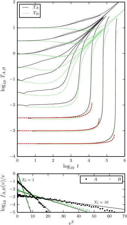
Figure 1: Growth of the mean kinetic energy in a 2D binary system of particles interacting via the non-reciprocal Hertzian forces (see text for details). The upper panel displays the time dependence of the temperatures $T_{A}$ and $T_{B}$. The solid lines show the development obtained from the simulations for the areal fraction $\phi=\pi r_{0}^{2}n=0.3$ and different initial temperatures $T_{0}$. All curves approach the universal asymptotes $\propto t^{2/3}$ described by Eqs. (15) and (16). The doted lines represent the solution of Eq. (13) for $T_{0}\gtrsim 1$. The early development at $T_{0}\ll 1$ is fitted by the explosive solution, Eq. (18), shown by the dashed lines. The temperatures are normalized by $\varphi_{0}$, time is in units of $\sqrt{mr_{0}^{2}/\varphi_{0}}$. The lower panel illustrates the velocity distributions $f_{A,B}(v)$ at $t\simeq 700$ for $T_{0}=1$ and 10.

For the “constant” non-reciprocity, $F_{\rm n}(r)/F_{\rm r}(r)=\Delta$, we get $\Delta_{\rm eff}=\Delta$ and $\epsilon=0$. In this case Eq. (13) yields the equilibrium $\dot{T}_{A,B}=0$ for the temperature ratio given by Eq. (9). Otherwise we have $\epsilon>0$ and the temperatures grow with time, approaching the asymptotic solution,

$$t\to\infty:\quad T_{A}(t)=\tau T_{B}(t)=ct^{2/3},$$ (15)

where $c\propto(nI_{\rm rr})^{2/3}$ and

$$\tau=\sqrt{\frac{(1+\Delta_{\rm eff})^{2}+\epsilon}{(1-\Delta_{\rm eff})^{2}+\epsilon}}.$$ (16)

Thus, the asymptotic temperature ratio is a constant which tends to the equilibrium value [Eq. (9)] for $\epsilon\to 0$.

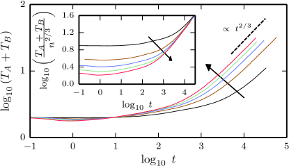
Figure 2: Time dependence of the total kinetic energy, $T_{A}+T_{B}$, obtained from the simulations. The development for $T_{0}=1$ and different $\phi$ (0.1, 0.3, 0.5, 0.7, 0.9, increasing along the arrow) is shown. The inset demonstrates the $\propto n^{2/3}$ density scaling of the asymptotic temperature growth. The temperature and time units are the same as in Fig. 1.

To verify the analytical results, we carried out a molecular dynamics simulation of a 2D binary, equimolar mixture of soft spheres. We implemented the velocity Verlet algorithm Swope82 with an adaptive time step. The simulation box with periodic boundary conditions contained $2\times 20,000$ particles with equal masses. We used a model Hertzian potential note2 ; Pamies09 ; Berthier10 whose reciprocal and non-reciprocal parts are given by $\varphi_{\rm r}(r)=\frac{1}{2}\varphi_{0}(\max\{0,1-r/r_{0}\})^{2}$ and $\varphi_{\rm n}(r)=\frac{1}{3}\varphi_{0}(\max\{0,1-r/r_{0}\})^{3}$, respectively, where $\varphi_{0}$ is the interaction energy scale and $r_{0}$ is the interaction range. At $t=0$ the particles were arranged into two interpenetrating square lattices with the initial temperature $T_{A}=T_{B}=T_{0}$ (therefore, at early simulation time a certain fraction of $T_{0}$ was converted into the interaction energy).

The numerical results are illustrated in Fig. 1, where we plot the dependencies $T_{A,B}(t)$ for different $T_{0}$. For the Hertzian interactions, from Eq. (14) we obtain $\Delta_{\rm eff}=0.57$ and $\epsilon=0.082$, and Eq. (16) yields the asymptotic temperature ratio $\tau=3.1$. One can see that for all $T_{0}$ the numerical curves approach the expected universal asymptotes described by Eqs. (15) and (16). Note that the early development at sufficiently low temperatures exhibits a remarkably sharp dependence on $T_{0}$ – we observe the formation of a plateau which broadens dramatically with decreasing $T_{0}$. On the other hand, for $T_{0}\gtrsim 1$ the numerical results are very well reproduced by the solution of Eq. (13), as expected. A small ($<10\%$) deviation observed in this case is due to the fact that weak collisions are no longer providing efficient Maxwellization of the velocity distribution for the “hotter” species $A$ (see the lower panel of Fig. 1).

In Fig. 2 we show how the temperature evolution depends on the density $n$. Here, the total kinetic energy $T_{A}(t)+T_{B}(t)$ calculated for different values of the areal fraction $\phi=\pi r_{0}^{2}n$ is plotted. In contrast to the sharp dependence on $T_{0}$ seen in Fig. 1, the increase of $n$ is accompanied by an approximately proportional shortening of the plateau note3 . The inset demonstrates the predicted $\propto n^{2/3}$ scaling for the asymptotic temperature growth.

In order to explain the observed behavior at low temperatures, we point out that the approximation of small-angle scattering is not applicable in this regime and, hence, Eq. (13) is no longer valid. Strong correlations make the analysis rather complicated in this case, but one can implement a simple phenomenological model to understand the essential features. We postulate that at sufficiently low temperatures the energy growth caused by non-reciprocal interactions can be balanced by nonlinearity, forming a “dynamical potential well” where the system can reside for a long time. Qualitatively, one can then expect the development around the initial temperature to be governed by the activation processes, and introduce the effective “Arrhenius rate” characterizing these processes. Assuming the dimensionless temperature $T$ (normalized by the effective depth of the well) to be small, we employ the following model equation:

$$\dot{T}=C\exp(T^{-\gamma}),$$ (17)

where $C$ is a constant (possible power-law factors can be neglected for $T\ll 1$) and $\gamma$ is an exponent determined by the particular form the potential well. Substituting $T^{-\gamma}\simeq T_{0}^{-\gamma}-\gamma T_{0}^{-\gamma-1}(T-T_{0})$ in Eq. (17) yields the explosive solution,

$$T(t)=T_{0}-\frac{T_{0}^{\gamma+1}}{\gamma}\ln\left[1-\frac{C\gamma}{T_{0}^{\gamma+1}}\exp(-T_{0}^{-\gamma})t\right],$$ (18)

with the explosion time $t_{\rm ex}=(T_{0}^{\gamma+1}/C\gamma)\exp(T_{0}^{-\gamma})$. In Fig. 1 we show that the explosive solution provides quite a reasonable fit to the numerical results at low temperatures for $C=4\times 10^{-5}$ and $\gamma=0.305$.

Let us briefly discuss the effect of dissipation due to friction against the surrounding medium. To take this into account, one has to add the dissipation term $-2\nu_{A,B}(T_{A,B}-T_{\rm b})$ to the r.h.s. of Eq. (13), where $\nu_{\alpha}$ is the respective damping rate in the friction force $-m_{\alpha}\nu_{\alpha}{\bf v}_{\alpha}$ and $T_{\rm b}$ is the background temperature (determined by the interaction of individual particles with the medium) Morfill09 ; vanKampen . In this case the temperatures $T_{A,B}$ always reach a steady state, since the growth term in Eq. (13) decreases with temperature. The resulting steady-state temperature ratio, $\tau_{\nu}$, can be easily derived from Eq. (13), assuming that the steady-state temperatures are much larger than $T_{\rm b}$. For similar particles, this requires the condition $\nu\ll nI_{\rm rr}/\sqrt{mT_{\rm b}^{3}}$ to be satisfied note4 . Then we obtain the following equation for $\tau_{\nu}$:

$$\tilde{\nu}[(1-\Delta_{\rm eff})^{2}+\epsilon]\tau_{\nu}^{2}-(\tilde{\nu}-1)(1-\Delta_{\rm eff}^{2}+\epsilon)\tau_{\nu}=(1+\Delta_{\rm eff})^{2}+\epsilon,$$

where $\tilde{\nu}=\nu_{A}/\nu_{B}$. For $\tilde{\nu}=1$ we get $\tau_{\nu}=\tau$, i.e., the steady-state temperature ratio is not affected by friction. Generally, $\tau_{\nu}$ exhibits a very weak dependence on $\tilde{\nu}$: e.g., for the Hertzian interactions the deviation between $\tau_{\nu}$ and $\tau$ is within $\simeq 1\%$ in the range $0.8\leq\tilde{\nu}\leq 1.3$ (expected for experiments with binary complex plasmas Morfill09 ; Comm ).

Note that at low temperatures the system can be dynamically “arrested” due to friction and never reach the asymptotic stage described by Eqs. (15) and (16). A simple analysis of Eq. (17) with the dissipation term shows that the arrest occurs when $\nu t_{\rm ex}\gtrsim 1$.

In conclusion, the presented results provide a basic classification of many-body systems with non-reciprocal interactions. We investigated different non-reciprocity classes in 2D and 3D systems which are relevant to a plethora of real situations: For instance, the shadow interactions Tsytovich97 ; Chaudhuri11 in binary complex plasmas have a constant non-reciprocity and can dominate the kinetics of 3D systems, while the wake-mediated interactions Morfill09 ; Couedel10 governing the action-reaction symmetry breaking in bilayer complex plasmas are generally characterized by a variable non-reciprocity. We expect that our predictions can be verified in complex plasma experiments, e.g., by measuring the kinetic temperatures in 2D binary mixtures or in 3D clouds under microgravity conditions. Furthermore, the analysis of dynamical correlations in the strong-damping regime should help to understand the effect of non-reciprocal effective interactions operating in colloidal suspensions.

The authors acknowledge support from the European Research Council under the European Union’s Seventh Framework Programme, Grant Agreement No. 267499.

References

- (1) J. N. Israelachvili, Intermolecular and Surface Forces (Elsevier, Amsterdam, 1992).
- (2) M. Dijkstra, R. van Roij, and R. Evans, J. Chem. Phys. 113, 4799 (2000).
- (3) P. G. Bolhuis, A. A. Louis, J. P. Hansen, and E. J. Meijer, J. Chem. Phys. 114, 4296 (2001).
- (4) M. Praprotnik, L. Delle Site, and K. Kremer, Annu. Rev. Phys. Chem. 59, 545 (2008).
- (5) B. M. Mognetti, P. Virnau, L. Yelash, W. Paul, K. Binder, M. Muller, and L. G. MacDowell, J. Chem. Phys. 130, 044101 (2009).
- (6) K. Hayashi and S. Sasa, J. Phys. Cond. Matter 18, 2825 (2006).
- (7) P. R. Buenzli and R. Soto, Phys. Rev. E 78, 020102 (2008).
- (8) K. Dholakia and P. Zemanek, Rev. Mod. Phys. 82, 1767 (2010).
- (9) B. Sabass and U. Seifert, Phys. Rev. Lett. 105, 218103 (2010).
- (10) R. Soto and R. Golestanian, Phys. Rev. Lett. 112, 068301 (2014).
- (11) J. Dzubiella, H. Löwen, and C. N. Likos, Phys. Rev. Lett. 91, 248301 (2003).
- (12) A. S. Khair and J. F. Brady, Proc. R. Soc. A 463, 223 (2007).
- (13) C. Mejia-Monasterio and G. Oshanin, Soft Matter 7, 993 (2011).
- (14) I. Sriram and E. M. Furst, Soft Matter 8, 3335 (2012).
- (15) V. N. Tsytovich, Phys. Usp. 40, 53 (1997).
- (16) S. A. Khrapak, A. V. Ivlev, and G. E. Morfill, Phys. Rev. E 64, 046403 (2001).
- (17) M. Chaudhuri, A. V. Ivlev, S. A. Khrapak, H. M. Thomas, and G. E. Morfill, Soft Matter 7, 1229 (2011).
- (18) A. Melzer, V. A. Schweigert, and A. Piel, Phys. Rev. Lett. 83, 3194 (1999).
- (19) G. E. Morfill and A. V. Ivlev, Rev. Mod. Phys. 81, 1353 (2009).
- (20) L. Couëdel, V. Nosenko, A. V. Ivlev, S. K. Zhdanov, H. M. Thomas, and G. E. Morfill, Phys. Rev. Lett. 104, 195001 (2010).
- (21) D. Helbing and P. Molnar, Phys. Rev. E 51, 4282 (1995).
- (22) D. Helbing, I. Farkas, and T. Vicsek, Nature 407, 487 (2000).
- (23) For the and pairs is the same, to distinguish the effect of non-reciprocity.
- (24) For 3D systems the corresponding expressions are easily derived using the cosine rule of spherical trigonometry.
- (25) L. D. Landau and E. M. Lifshitz, Mechanics (Pergamon, Oxford, 1976).
- (26) E. M. Lifshitz and L. P. Pitaevskii, Physical Kinetics (Pergamon, Oxford, 1981).
- (27) L. Spitzer, Physics of Fully Ionized Gases (Dover, New York, 2006).
- (28) W. C. Swope, H. C. Andersen, P. H. Berens, and K. R. Wilson, J. Chem. Phys. 76, 637 (1982).
- (29) We chose the Hertzian forces for the illustration, in order to ensure precise numerical calculations at low and high temperatures.
- (30) J. C. Pamies, A. Cacciuto, and D. Frenkel, J. Chem. Phys. 131, 044514 (2009).
- (31) L. Berthier, A. J. Moreno, and G. Szamel, Phys. Rev. E 82, 060501 (2010).
- (32) A small dip in the early development (Fig. 2) is due to partial conversion of the initial kinetic energy into the interaction energy.
- (33) N. G. van Kampen, Stochastic Processes in Physics and Chemistry (Elsevier, Amsterdam, 1981).
- (34) This strong inequality always holds for typical experiments with 2D complex plasmas, where the interparticle interaction can be approximated by the Yukawa potential, , so that .
- (35) C. Du, private communication (2013).