Satellite abundances around bright isolated galaxies II: radial distribution and environmental effects

Abstract

We use the SDSS/DR8 galaxy sample to study the radial distribution of satellite galaxies around isolated primaries, comparing to semi-analytic models of galaxy formation based on the Millennium and Millennium-II simulations. SDSS satellites behave differently around high- and low-mass primaries: those orbiting objects with $M_{*}>10^{11}M_{\odot}$ are mostly red and are less concentrated towards their host than the inferred dark matter halo, an effect that is very pronounced for the few blue satellites. On the other hand, less massive primaries have steeper satellite profiles that agree quite well with the expected dark matter distribution and are dominated by blue satellites, even in the inner regions where strong environmental effects are expected. In fact, such effects appear to be strong only for primaries with $M_{*}>10^{11}M_{\odot}$. This behaviour is not reproduced by current semi-analytic simulations, where satellite profiles always parallel those of the dark matter and satellite populations are predominantly red for primaries of all masses. The disagreement with SDSS suggests that environmental effects are too efficient in the models. Modifying the treatment of environmental and star formation processes can substantially increase the fraction of blue satellites, but their radial distribution remains significantly shallower than observed. It seems that most satellites of low-mass primaries can continue to form stars even after orbiting within their joint halo for 5 Gyr or more.

1 Introduction

Satellite galaxies can contribute substantially to our understanding of galaxy formation. In the current structure formation paradigm, galaxies form by the cooling and condensation of gas at the centres of an evolving population of dark matter halos that are an order of magnitude larger in both mass and linear size than the visible galaxies (White & Rees, 1978). Comparable contributions to the growth of such halos come from smooth accretion of diffuse matter and from mergers with other halos spread over a very wide range in mass (Wang et al., 2011). The more massive accreting halos will normally have their own central galaxies, and after infall these become “satellites” of the galaxy at the centre of the dominant halo, orbiting it within their own “subhalos”. Later, the satellites may merge with the central galaxy and so contribute to its growth.

High-resolution cosmological simulations predict not only the masses, positions and velocities of dark matter halos but also those of the subhalos they contain (e.g. Moore et al., 1999; Gao et al., 2004; Springel et al., 2008; Gao et al., 2008, 2011). Linking such data over time then allows construction of the assembly history of every system in the simulated volume. In combination with a model for galaxy formation, such halo/subhalo merger trees can be used to predict the development of the full galaxy population in the region considered. This can be compared directly with properties of observed populations such as abundances, scaling relations, clustering and evolution (e.g. Springel et al., 2001; Bower et al., 2006; Croton et al., 2006; Guo et al., 2011). A particular strength of such “semi-analytic” population simulations is that they enable evaluation of the relative sensitivity of these observables to cosmological and to galaxy formation parameters (e.g. Wang et al., 2008; Guo et al., 2013). Satellite galaxies play an important role in such work because they are particularly sensitive to environmental effects and to the assembly history of halos.

In Wang & White (2012, PaperI hereafter) we used the Sloan Digital Sky Survey (SDSS) to study the luminosity, mass and colour distributions of satellite galaxies as a function of the properties of their host. A comparison of our observational results to semi-analytic galaxy formation simulations within the concordance $\Lambda$CDM cosmology showed good overall agreement for satellite abundances, inspiring some confidence in the realism of the particular galaxy formation model used (from Guo et al., 2011), but large discrepancies for satellite colour distributions confirmed earlier demonstrations that such models substantially overestimate the environmental suppression of star formation (e.g. Font et al., 2008; Weinmann et al., 2009). In this paper we extend our earlier work through a detailed analysis of the radial distribution of satellites around their hosts. This enables further exploration both of the successes and of the failures of the galaxy formation model.

The observational study of satellite number density profiles benefited enormously from the advent of wide-angle spectroscopic surveys such as the Two Degree Field Galaxy Redshift Survey (2dFGRS, Colless et al., 2001) and the SDSS (York et al., 2000). The availability of redshift measurements for almost all objects above some apparent magnitude limit allows the full three-dimensional distribution of objects to be studied (although in “redshift space” rather than true position space) greatly facilitating the identification of host/satellite systems. Several studies concluded that the mean radial satellite distribution in such spectroscopic samples can be fit (in projection) by a power-law $\Sigma_{\rm sat}\propto r^{-\alpha}$, although the range of indices quoted is quite broad $\alpha\sim 0.9$ to $1.7$ (Sales & Lambas, 2005; van den Bosch et al., 2005; Chen et al., 2006; Chen, 2008). There is some indication that this index correlates with the properties of the primaries and/or satellites under consideration, but results are also rather noisy because of the relatively bright lower limit on the luminosity of the satellites which is enforced by the spectroscopic apparent magnitude limit.

In addition to being restricted to relatively bright objects, spectroscopic satellite samples are also subject to selection effects such as redshift incompleteness due to fibre-fibre collisions and survey geometry constraints which particularly affect their coverage of close pairs. In this context, photometric samples offer an interesting alternative, since they are complete at all separations and to apparent magnitude limits which are typically $3-4$ magnitudes fainter than the corresponding spectroscopic surveys. For example, the SDSS/DR8 data are effectively complete to $r$-band magnitudes $m_{r}=17.7$ and $m_{r}=21$ for the spectroscopic and photometric catalogues, respectively (Aihara et al., 2011).

Inspired by this, several groups have recently analyzed primary/satellite samples, where the primary galaxies are selected from spectroscopic surveys, ensuring their distances and environments are well characterized, but their satellite populations are identified in deeper photometric data and so must be corrected statistically for the inevitable foreground and background contamination (e.g. Lares et al., 2011; Guo et al., 2012; Nierenberg et al., 2011, 2012; Jiang et al., 2012; Tal et al., 2012). This approach is reminiscent of the pioneering work in this field, where satellites were identified on photographic plates around relatively bright primary samples (Holmberg, 1969; Lorrimer et al., 1994). The projected satellite profiles measured in these hybrid studies are also consistent with power-laws $\Sigma_{\rm sat}\propto r^{-0.9,-1.2}$, and again correlations are seen between the slope of the profiles and the colour/mass/type of the primaries and satellites.

Despite this superficial agreement, there are large discrepancies between recently published studies of satellite radial distributions. Some authors find satellite profiles to be steeper than the NFW profile (Navarro et al., 1996, 1997) predicted for the dark matter (Watson et al., 2012; Tal et al., 2012; Guo et al., 2014); others consider them as good tracers of the dark matter (Nierenberg et al., 2012); yet others find them to be less concentrated than the dark halos they inhabit (Budzynski et al., 2012; Wojtak & Mamon, 2013). The trends found with intrinsic properties of satellites/primaries also disagree between studies. For instance, whereas Watson et al. and Tal et al. find that bright satellites have steeper profiles, Guo et al. and Budzynski et al. conclude that faint companions are more strongly concentrated. Nierenberg et al. find no variation in profile slope with satellite mass.

Some of this disagreement can plausibly be traced to differing sample definitions. For example, Tal et al. (2012) studied satellite profiles around Luminous Red Galaxies (LRGs) at $0.28<z<0.4$, whereas both Watson et al. (2012) and Guo et al. (2012) used SDSS Main Sample galaxies at lower redshifts. The redshift range probed by Nierenberg et al. (2012) is $0.1<z<0.8$, based on data from the deeper COSMOS survey, but their samples are relatively small so trends may be masked by counting noise. Furthermore, Tal et al. (2012) and Watson et al. (2012) studied satellite radial profiles down to very small separations ($r_{p}\sim 30$kpc) and their inference of a steeper than NFW distribution depends on these scales. Careful photometric corrections are needed in such work, because satellite magnitudes are systematically biased by their proximity to a much brighter central galaxy. Deblending and background estimation effects can be substantial in this situation and are quite uncertain (e.g. Mandelbaum et al., 2006). Not all authors apply such corrections (e.g. Guo et al., 2012) and in consequence their results at the smallest separations may be compromised.

Variations in the radial distribution of satellites as a function of primary or satellite properties provide important clues to the processes driving galaxy evolution, in particular, to the influence of environmental effects. Tidal disruption and ram-pressure stripping are believed to be the main agents of structural change in satellites once they have fallen into their host halos. Extended reservoirs of gas may be removed, causing the satellites to run out of fuel for star formation, or gas and stars may be removed directly from the visible regions of the galaxies. As a result, satellites are predicted to be less active and redder than otherwise similar galaxies in the field.

There is clear observational evidence for effects of this kind. Studies of galaxy correlations show enhanced clustering of red objects at fixed stellar mass (see e.g. Li et al., 2006; Zehavi et al., 2011) and there is a consensus among authors that the fraction of red and passive satellite galaxies is larger than for central galaxies of similar mass (see e.g. van den Bosch et al., 2008; Yang et al., 2009; Weinmann et al., 2009). There are also, however, clear indications that this increased red fraction among satellites is a function of the stellar or halo mass of the primary, suggesting that environmental effects are weak or even negligible for satellites orbiting low-mass primaries (e.g. Weinmann et al., 2006; Prescott et al., 2011; Wetzel et al., 2012).

Theoretical predictions based on semi-analytical models successfully reproduce several of these trends, but typically overproduce the fraction of red satellites (e.g. Coil et al., 2008). Recent improvements in the modelling of gas removal and tidal stripping have improved the situation (Font et al., 2008; Guo et al., 2011), but a significant problem still persists (Weinmann et al., 2011). The radial distributions of red and blue satellites and their relation to the properties of the primary galaxy give additional information about environmental influences on satellites, complementing the information provided by the relative abundances of the two populations.

Despite difficulties in matching the observed colour distribution, simulations have proven useful for interpreting the observed properties of satellite galaxies. Kravtsov et al. (2004) and Gao et al. (2004) used N-body simulations to argue that the observed radial distribution of luminous satellites is more easily understood if these objects populate the most massive subhalos at the time of infall, rather than the most massive today. The distribution of luminous satellites in both hydrodynamical and semi-analytic simulations suggests that they may be reasonable tracers of the underlying dark matter distribution of their host halo (e.g. Gao et al., 2004; Nagai & Kravtsov, 2005; Sales et al., 2007). Numerical simulations also show that the time of infall of satellites onto their host is correlated with their current distance from halo centre (e.g. Gao et al., 2004), a relation that becomes tighter if we consider satellite orbital binding energy (Rocha et al., 2012). Thus the radial distribution of satellites encodes information about the assembly of dark matter halos that is not otherwise observationally accessible.

In this paper we study the radial distribution of satellites in a hybrid primary/satellite sample selected from the spectroscopic + photometric SDSS/DR7 and DR8 catalogues. We go beyond previous work by comparing our results with a mock-galaxy catalogue generated from the Millennium and Millennium-II simulations (Springel et al., 2005; Boylan-Kolchin et al., 2009) using the semi-analytical model of Guo et al. (2011). The mock sample allows an improved assessment of the projection and sample selection effects, facilitating the physical interpretation of the observed profiles. At the same time, we are able to test the galaxy formation model by contrasting its predictions with observables it was not tuned to reproduce. This paper follows naturally from the analysis presented in Paper I which focused on the abundance and mass spectrum of satellites around isolated primaries.

This paper is organized as follows: our data sources and the selection criteria we apply to observed and simulated catalogues are described in Sec. 2. We report the trends found in the radial distribution of satellites according to primary/satellite colours and masses in Sec. 3.2 and 3.3, while we discuss the implications for environmental modulation of star formation in Sec. 4. We summarize and discuss our main conclusions in Sec. 5. Throughout this paper we adopt the cosmology of the original Millennium simulations ($H_{0}=73~{}\mathrm{km~{}s^{-1}}~{}\mathrm{Mpc}^{-1}$, $\Omega_{\rm m}=0.25$, $\Omega_{\Lambda}=0.75$, $n=1$). A discussion of the effect of cosmology on the satellite properties presented in this paper is included in Sec. 4.

Table 1: Average halo virial radius $r_{\rm vir}$ (following G11), scale radius $r_{s}$ (following Zhao et al. 2009), inner radius $r_{\mathrm{inner}}$ and the $(g-r)$ colour cut separating blue from red satellites for the five primary stellar mass bins considered in our study. The final row gives the number of red and blue SDSS primaries in each of these bins.

$\log M_{*}/M_{\odot}$	11.4-11.7	11.1-11.4	10.8-11.1	10.5-10.8	10.2-10.5
$r_{\rm vir}$ [kpc]	725	430	270	210	170
$r_{s}$ [kpc]	156.6	74.4	39.3	27.1	21.0
$r_{\mathrm{inner}}$ [kpc]	50	50	30	20	10
$(g-r)_{\rm SDSS}$	0.840	0.830	0.820	0.811	0.801
$(g-r)_{\rm mock}$	0.627	0.618	0.609	0.600	0.591
$N_{\mathrm{SDSS}}$ [red, blue]	1651, 35	6170, 731	8518, 4142	5453, 5953	1625,3764

2 Data Selection

In this paper we use the same primary and satellite samples as in Paper I. In the following, we briefly introduce the underlying observational and simulation catalogues and the selection criteria which define our samples, referring the reader to Paper I for further details.

2.1 Identification of primary and satellite galaxies

We select isolated primary galaxies from the spectroscopic catalogue of the New York University Value Added Galaxy Catalogue (NYU-VAGC) , which is built by Blanton et al. (2005) based on the Seventh Data Release of the Sloan Digital Sky Survey (SDSS/DR7; Abazajian et al., 2009). Every galaxy with apparent (Petrosian) $r$-band magnitude brighter than $r=16.6$ is a primary candidate. To ensure isolation, it must fulfill two further conditions: it must $i)$ be at least one magnitude brighter than any companion within a projected radius of $r_{p}=0.5~{}{\rm Mpc}$ and a line-of-sight velocity difference $|\Delta{z}|<1000$ km/s, and $ii)$ be the brightest object within $r_{p}<1~{}{\rm Mpc}$ and $|\Delta{z}|<1000$ km/s. This returns 66,285 isolated primaries.

The SDSS spectroscopic sample is incomplete due to fibre-fibre collision. For our selection criteria we expect $\sim$91.5% completeness on average, varying with position on the sky and worse in dense regions such as the centres of galaxy groups or clusters. To ensure that none of our primaries is falsely identified as isolated due to incompleteness in the spectroscopic survey, we look for further companions using the photometric SDSS catalogue. In practice, we will reject a primary candidate if it has a photometric companion satisfying the position and magnitude cuts of i) and ii) which is absent from the spectroscopic catalogue but whose probability to have a redshift equal or less than the primary is larger than $10\%$. For this last step we use the photometric redshift distributions from Cunha et al. (2009). This reduces our sample of isolated primaries to 41,883 candidates. Lastly, we also consider survey boundaries to ensure that most of the companions of our primaries fall within the SDSS footprint. We use the spherical polygons provided on the NYU-VAGC website to quantify the survey boundaries and masked areas around bright stars. We remove from the above primary sample all candidates for which more than 20% of a surrounding disk with $r_{p}<1\rm Mpc$ lies outside the SDSS footprint. About 1.5% galaxies are removed through this procedure, leading to our final primary sample with 41271 isolated systems.

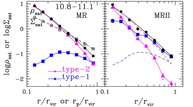
Figure 1: The radial distribution of satellites with $\log M_{*}/M_{\odot}>9.0$ in semi-analytic catalogues based on the Millennium (left) and Millennium-II (right) simulations. Only isolated primaries in the stellar mass range $10.8<\log M_{*}/M_{\odot}<11.1$ are considered. Error bars are obtained from the scatter among 100 bootstrap re-sampled realizations of primaries, and are smaller than the marker size in most cases. Solid black dots show the average 3D radial profile of satellites as a function of $r/r_{\rm vir}$. The distribution is well reproduced in both panels by an NFW profile with arbitrary normalization and the mean concentration of the host dark matter halos (the black solid curve which is identical in the two panels). In each panel, the total profile is split into contributions from satellite galaxies that still retain a dark matter subhalo (blue solid squares) and from “orphan” galaxies that are followed by the simulation even though their associated subhalo has been tidally disrupted (magenta solid triangles). Orphans dominate the satellite population in the Millennium but are important only in the inner regions of Millennium-II halos, reflecting its 125 times better mass resolution. The data from the left panel are repeated as dashed blue and magenta curves in the right panel. It is remarkable that the total satellite populations agree well between the two simulations despite the very different contribution of orphans in the two cases. Note also that orphans sill dominate in the inner regions even at MS-II resolution. Black empty circles in the left panel show the 2D radial distribution of satellites as a function of the projected distance $r_{p}/r_{\rm 200}$. This also follows well the projected NFW profile expected for the host dark matter halos (black dashed line).

Satellites are identified in the SDSS/DR8 photometric catalogue (Aihara et al., 2011) and are corrected statistically for background contamination (see Paper I for details). We proceed as follows. For each isolated primary we compute, as a function of projected distance $r_{p}$, the number of objects with apparent magnitude $r$ and colour $(g$-$r)$ in SDSS/DR8. For completeness, we only consider objects brighter than $r=21$ (model magnitudes). For each bin in distance $r_{p}$, we subtract the average number of galaxies in the $(r,g$-$r)$ bin expected in this area of the sky, as estimated from the survey as a whole. The excess counts with respect to an homogeneous galaxy background are assumed to be satellites physically associated with the primary galaxy. Rest-frame colours and stellar masses can then be computed for these satellites by assigning them the redshift of the primary. Finally, results for different primaries can be averaged after making completeness, volume and edge corrections as set out in Paper I.

To aid the physical interpretation of these data, we use mock galaxy catalogues generated from the Millennium and Millennium-II simulations (Springel et al., 2005; Boylan-Kolchin et al., 2009). The formation of galaxies is simulated using the semi-analytic model of Guo et al. (2011) (hereafter G11). This is tuned to reproduce SDSS estimates of the mass and luminosity functions of low-redshift galaxies and also fits the measured autocorrelations of SDSS galaxies at high stellar mass. Autocorrelations of lower mass galaxies are significantly overestimated on small scales ($r_{p}<1.0~{}{\rm Mpc}$) but the abundances of satellites around primaries of the mass considered in this paper are in quite good agreement with direct measurements from SDSS (see Paper I). We create simulated galaxy catalogues by projecting the simulation “boxes” in three orthogonal directions, i.e. parallel to their $x$, $y$ and $z$ axes. In each projection we assign every galaxy a redshift based on its “line-of-sight” distance and peculiar velocity. We can then apply similar isolation criteria as in SDSS to identify a set of simulated primaries.

In addition, we analyze a sample of primary and satellite galaxies derived from a “light-cone” mock catalogue which mimics incompleteness due to fibre collisions as well the survey geometry of SDSS/DR7 (Henriques et al., 2012). This allows us to apply exactly the same selection criteria as described above for the SDSS sample and to compare with the simple projections used for our main analysis (which provide better counting statistics). Results of this comparison are shown in an Appendix.

Figure 2: Projected number density profiles for satellites brighter than $r$-band apparent magnitude $r=21$ and for primaries in different stellar mass bins (the quoted numbers indicate the interval in $\log M_{*}/M_{\odot}$). The profiles correspond to the satellite number counts per primary and per unit surface area that we indicate in the y-axis with units $N^{-1}$ and $D=r_{p}/r_{\mathrm{vir}}$, respectively. Dashed lines indicate the expected distribution of dark matter around the hosts, computed by projecting the average NFW profile with mass following the $M_{*}-M_{\rm vir}$ relation from G11 and concentration from Zhao et al. (2009). The shape of the distribution of SDSS satellites (left column) varies with primary stellar mass: for satellites of low-mass centrals ($\log M_{*}/M_{\odot}<11.1$) the profile agrees well with the expected dark matter distribution. In contrast, satellites of the most massive primaries have a noticeably shallower distribution than predicted for the dark matter. Error bars are almost invisible and correspond to the scatter among 100 bootstrap re-samplings of each primary sample. For comparison, the right column shows results of a similar analysis performed on our simulation catalogue. Satellites are here counted down to an $r$-band absolute magnitude corresponding to $r=21$ at the median redshift of the SDSS primaries in the corresponding left-hand panel. Note the excellent agreement in the absolute numbers of satellites in SDSS and in the simulation. The dependence of the shape of the satellite profiles on primary stellar mass is not, however, present in the simulation where satellites trace the underlying dark matter distribution regardless of primary stellar mass.

Figure 3: Projected number density profiles for satellites in SDSS split according to satellite stellar mass: $\log M_{*}/M_{\odot}=[10.2,11.2],[9.2,10.2]$ and $[8.2,9.2]$ from left to right. Samples divided by satellite stellar mass require the use of volume-limited samples, unlike Fig. 2. For a given primary mass bin, we find no strong dependence of satellite profiles with satellite stellar mass. Simulated satellites show a similar behaviour in the mock catalogue but are not shown here.

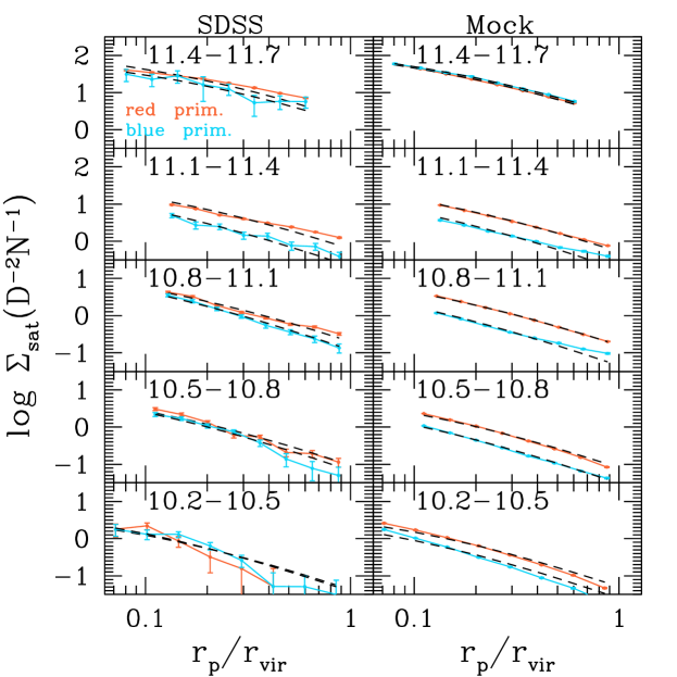
Figure 4: As Fig. 2 but split according to primary colour; results for red primaries are shown in orange and for blue primaries in light-blue. As before, left and right columns show results from the SDSS and from the simulations, respectively. Black dashed curves are predicted NFW profiles for the host dark matter halos, re-normalized to fit the data. The overall shape of the satellite distribution does not depend on primary colour, except for the two most massive primary bins for SDSS, where the red primaries show slightly flatter profiles than the blue. Red primaries have a larger abundance of satellites at all radii, an effect that is more pronounced in the mock catalogue than in the SDSS.

2.2 Satellite number density profiles

The background subtraction method explained above provides a measure of the cumulative number of satellites in fine grids of projected distance in the range $r_{p}=[0,0.5]\rm Mpc$. We group this data according to primary mass and colour (Sec. 3.2) and to satellite mass and colour (Sec. 3.3) in order to study the average projected number density profile of satellites, $\Sigma_{\rm sat}$, defined as the mean number of satellites in some chosen magnitude range per primary and per unit area as a function of projected distance from the primary. Uncertainties are estimated from bootstrap re-samplings of each primary sample. Following Paper I, we divide our primaries into 5 disjoint stellar mass bins: $\log M_{*}/M_{\odot}=[10.2-10.5]$, $[10.5-10.8]$, $[10.8-11.1]$, $[11.1,11.4]$ and $[11.4-11.7]$.

For every primary stellar mass bins, we consider 8 equal-size logarithmic radial bins that extend up to the average virial radius, $r_{\rm vir}$, of the subsample (see Table 1). We estimate virial quantities using the relation between mean halo mass and primary stellar mass for all the isolated primaries in our semi-analytic catalogue. In SDSS the luminosity of the primary galaxy affects the detectability of faint satellites at small projected radii. We thus exclude the very central regions and measure $\Sigma_{\rm sat}$ in the radial range $r_{\rm in}<r_{p}<r_{\rm vir}$, where $r_{\rm in}$ depends on primary stellar mass as given in Table LABEL:tbl:primaries. The average virial radius for the most massive primary stellar mass bins is 725 kpc and is thus larger than 500 kpc, the projected radius within which we require that our primary galaxies be at least one magnitudes brighter than any neighbour. This induces a feature in the satellite profile at this radius, so below we present profiles for this largest primary stellar mass bin only over the range $50~{}{\rm kpc}<r_{p}<500~{}{\rm kpc}$.

When considering the whole satellite population, we include as many satellites as we can by going down to the flux limit, $r=21$. This limit corresponds to different (intrinsic) satellite luminosities and masses according to the redshift of the primary and the colour of the satellite. Although by working with a flux-limited sample we are including satellites of different masses for primaries at different redshifts, this does not appreciably affect the global shape of the satellite distribution we measure, because, as we show in Sec. 3.1 and 3.3, there is only a very weak dependence of $\Sigma_{\rm sat}$ on satellite stellar mass for primaries in the mass range we consider.

When our analysis requires us to split satellites according to their stellar mass and colour, we proceed as follows. Since satellites are selected from the photometric catalogue, we assume they have the same redshift as their primary galaxy, allowing us to convert observed apparent magnitudes and colours into rest-frame quantities. With these, we estimate the stellar mass of the apparent companions according to:

$$(M/L)_{r}=-1.0819^{0.1}(g-r)^{2}+4.1183^{0.1}(g-r)-0.7837.$$ (1)

which is obtained through a fit to a flux-limited ($r<17.6$) galaxy sample from the NYU-VAGC. Stellar masses in the sample were estimated by fitting stellar population synthesis models to the K-corrected galaxy colours assuming a Chabrier (2003) initial mass function as in Blanton & Roweis (2007).

Notice that in contrast to the case when we take all satellites down to the magnitude limit, when computing satellite number density profiles as a function of satellite mass we need to account properly for completeness limitations. In these cases we proceed as in Paper I: a primary is allowed to contribute counts to a given bin in satellite mass only if the K-corrected absolute luminosity corresponding to $r=21$ for a galaxy at the redshift of the primary and lying on the red envelope of the intrinsic colour distribution is fainter than the lower luminosity limit of the bin.

Finally we note that our primary selection criteria result in a sample of galaxies which are usually but not always the central galaxies of their dark matter halos. In our simulated catalogue, the fraction of primaries which are not the central object of their friends-of-friends (FoF) dark matter halo is 0.1006, 0.1021, 0.0733, 0.0410 and 0.0156 for our five primary stellar mass bins (from most massive to least massive). This fraction increases strongly with primary stellar mass because of the concomitant increase in halo size (see Table 1). Note that the great majority (80 to 90 percent) of these non-central primaries actually lie outside the virial radius of the FoF halo of which they are formally a satellite.

3 Results

Throughout this paper we will make extensive use of comparisons between results for the SDSS and for our simulated galaxy populations. Before starting systematic presentation and interpretation of the observed satellite profiles, we therefore use our two large simulations to demonstrate that the relevant quantities are numerically converged and that the observed, projected radial profile of satellites is related as expected to the mean three-dimensional distribution around the primary galaxies. For brevity, we focus on primaries with stellar mass in the range, $10.8<\log M_{*}/M_{\odot}<11.1$ and satellites more massive than $\log M_{*}/M_{\odot}>9$ , but we emphasize that we have checked explicitly that similar results are found for other choices of primary and satellite mass, as well as for samples split by primary or satellite colour.

Fig. 1 shows the 3D and 2D satellite number density profiles in the Millennium and Millennium-II simulations. In both panels, solid black dots show the three-dimensional number density of satellites as a function of distance $r$ from their primary, normalized to the average $r_{\rm vir}=270$ kpc for primaries of this stellar mass (see Table LABEL:tbl:primaries). These measurements agree essentially perfectly given the counting statistics (there are 125 times fewer primaries in the MS-II) and are very well represented by an NFW profile (black solid line) with concentration parameter $c=6.87$, the value expected for halos of virial mass $M_{\rm vir}=10^{12.5}\rm M_{\odot}$ (Zhao et al., 2009), which is the mean halo mass for simulated primaries in this stellar mass bin.

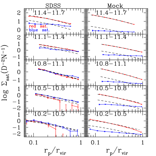
Figure 5: Satellite number density profiles split according to satellite colour. Red and blue curves refer to red and blue satellites, respectively. Primaries are grouped by their stellar mass as before (rows). In the observed sample (left), the radial profile of red and blue satellites varies with primary stellar mass. For massive primaries, blue satellites have significantly shallower profiles than the red population and also than predicted for the dark matter (black dashed curves). However, for primaries with $\log M_{*}/M_{\odot}<11.1$, red and blue satellites have comparably steep profiles, which are similar to that expected for the dark matter. Blue satellites dominate in number at all radii for these lower mass primaries. The semi-analytic catalogue (right column) fails to reproduce many of these trends: blue satellites in the model always have a very shallow radial profile and are sub-dominant for all primary stellar masses. Environmental effects are apparently too strong in the semi-analytic model, particularly in low-mass halos. Red satellite profiles are similar to the dark matter predictions at all masses both in SDSS and in the simulations.

In the simulations there are two different kinds of satellites which combine to give these number density profiles, those which have an associated dark matter subhalo (type-1, blue solid squares in Fig. 1) and those whose dark matter subhalo has fallen below the resolution limit of the simulation (type-2, magenta solid triangles). The positions and velocities of the the latter “orphan” galaxies are set to the current values for the particles which were the most bound at the centre of their subhalos at the last time these were identified in the simulation. Orphan galaxies are removed from the galaxy catalogues when one of two conditions is fulfilled: either the time since disruption of the subhalo exceeds the time estimated for dynamical friction to cause a merger with the primary, or the estimated tidal forces from the host exceed the binding energy of the satellite so that it is disrupted (see G11 for further details.)

In the Millennium Simulation (the left panel of Fig. 1), satellites with a dark matter subhalo are comparable in number to the orphans only near the virial radius. Throughout the inner halo, satellite numbers are entirely dominated by orphans. In the Millennium-II, however, (the right panel) orphans are much less numerous and dominate the population only at the smallest radii ($r<0.2r_{\rm vir}$). To facilitate a direct comparison, we repeat the type-1 and type-2 data from the left panel as dashed blue and magenta lines in the right panel. The increase in mass resolution in the MS-II increases the number of satellites with resolved subhalos by factors between 3 and 30 in the inner halo and reduces the number of orphans to compensate. Despite this, the total number of satellites agrees very well and their profile is very similar to that of the dark matter. Note that even at the high resolution of MS-II it is important to include the orphans to get a reliable and numerically converged estimate of the number density profile. Similar conclusions were drawn by G11 and by Guo & White (2014) from the study of small scale correlations and by Moster et al. (2010) from their abundance matching work.

Fig. 1 also explores projection effects in the model. Black empty dots in the left panel show the average profile obtained when systems are projected along their $x$, $y$ and $z$ axes. In practice, we count all apparent companions around our primaries and correct statistically for unassociated objects that happen to be projected near them, based on the mean surface number density of galaxies times the area of each annular bin. This projected number density profile, $\Sigma_{\rm sat}$, is also shown as a function of projected distance $r_{p}$ normalized to $r_{\rm vir}$, and again is very well represented by an NFW fit to the (projected) dark matter distribution (dashed black line). Thus, the simulations suggest that satellite profiles should closely parallel the mean dark matter distributions around isolated galaxies, a result that could be checked directly using galaxy-galaxy lensing.

In what follows we will study projected number density profiles of satellites around isolated SDSS galaxies, comparing directly with simulation results. We have checked that numerical convergence between the two simulations is as good as in Fig. 1 for all the other plots we show, and hence, unless otherwise stated, we show only results based on the Millennium Simulation, since these have better counting statistics.

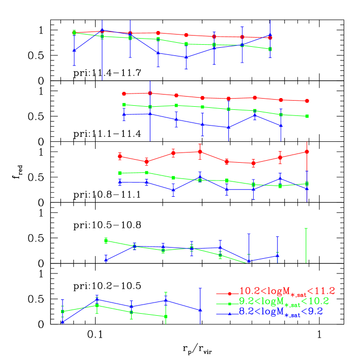
Figure 6: The fraction of red satellites, $f_{\rm red}$, as a function of projected distance from isolated SDSS primary galaxies. Each panel corresponds to primaries in a different range of $\log M_{*}/M_{\odot}$, as indicated. Results for satellites in three different stellar mass ranges are shown as curves of different colour. Red satellites are more common around high-mass primaries and also at smaller distances, although the trends with radius are rather weak. Error bars correspond to 100 bootstrap re-samplings of the primary samples.

3.1 Satellite number density profiles: dependence on primary stellar mass

The thick black lines in the left column of Fig. 2 show the mean projected number density of satellites around isolated SDSS primaries, $\Sigma_{\rm sat}$, as a function of projected separation ($r_{p}$), normalized by mean inferred virial radius ($D=r_{p}/r_{\mathrm{vir}}$). Each row corresponds to primaries in a different stellar mass range, as indicated by the listed values of $\log M_{*}/M_{\odot}$. Satellite number density profiles $\Sigma_{\rm sat}$ are computed by summing the satellite counts (after background correction) in each radial bin, and then dividing by the number of contributing primaries per mass bin (see Table LABEL:tbl:primaries). The error bars correspond to the dispersion among 100 bootstrap re-samplings of each primary sample. We maximize the statistics by including all satellites down to the apparent magnitude limit $m_{r}=21$ of the SDSS photometric catalogue. Because of the large number of satellites included (including background galaxies, there are about $\sim 7,000,000$ photometric companions projected within 500 kpc of these primaries), the error bars are almost invisible in most cases.

We find that the shape of satellite profiles around our isolated SDSS primaries depends significantly on primary stellar mass, with a shallower radial distribution around high-mass primaries than around primaries with $\log M_{*}/M_{\odot}<11.1$. This is most clearly seen by comparing with the expected mean dark matter profiles, which we indicate as dashed lines in each plot. These are computed by using the stellar mass of each primary to estimate its halo mass according to the mean $M_{*}$-$M_{200}$ relation in the semi-analytic catalogue of G11. We then compute the average halo mass in each bin and use the concentration-mass relation of Zhao et al. (2009) to get the mean projected NFW profile expected for the dark matter. Finally, we re-adjust the normalization to obtain a good fit to the amplitude of the simulation results in the right panel of each row (the dashed curves are identical in each pair of panels). We have explicitly checked that stacking the DM particles directly around the simulated galaxy sample gives almost identical results.

Massive primaries with $\log M_{*}/M_{\odot}>11.1$ show a satellite profile that is inconsistent with the predicted dark matter profile. In contrast, the satellite distribution agrees well with the predicted dark matter distribution around lower mass primaries. In the lowest mass bin (the bottom left panel) the satellite profile declines more steeply than the predicted dark matter profile at large radii. However, our tests indicate that at these radii the satellite counts around low-mass primaries become sensitive to background subtraction and are artificially steepened because our isolation criteria cause a slight suppression of the number of background galaxies around our primaries compared to randomly selected points on the sky. We show in the Appendix that the measured satellite profiles in a light-cone mock catalogue decline more steeply in the lowest mass bin than those measured directly from the projected simulation box. Such uncertainties in background subtraction do not affect our profile measurements at smaller radii or around more massive galaxies, because of the higher mean densities expected there.

The right column of Fig. 2 compares our SDSS results with analogous results for satellites surrounding isolated primaries in our mock catalogue based on the G11 simulation. For these plots, simulated satellites are counted down to an $r$-band absolute magnitude corresponding to $r=21$ at the median redshift of the SDSS primaries in the corresponding left panel. As noted above, the dashed curve in each panel is an NFW profile representing the mean halo mass distribution of the simulation primaries with its normalization adjusted to fit the satellite counts, and is identical to the curve overplotted on the SDSS data in the corresponding left panel. The excellent agreement in normalization in each pair of panels thus repeats the result of Paper I, that the G11 simulation does a good job in reproducing the observed abundance of satellites as a function of primary mass. However, in the simulation, satellites follow the dark matter distribution for primaries of all stellar masses. This is inconsistent with the shallower slope found for massive SDSS primaries.

This disagreement is puzzling in view of the good match between model and SDSS found by G11 for the small scale autocorrelations of massive galaxies, and the significantly poorer agreement in shape found for the autocorrelations of lower mass galaxies (see Fig. 20 in G11). Apparently, although massive primaries have the right spatial distribution in the mock catalogue, their satellites are somewhat too concentrated to small radii in comparison to SDSS. We show in the Appendix that more relaxed isolation criteria result in flatter satellite profiles in the outer regions (since satellites associated to other nearby primaries are now allowed to contribute), but the change is only significant for low/intermediate mass primaries. The overall shallower profile of satellites around massive primaries in SDSS seems robust to changes in isolation criteria and its physical explanation remains unclear. More efficient tidal disruption associated to massive primaries could provide a viable explanation for the inner shallow slopes. More definitive conclusions will require a better treatment of this process in the models, together, perhaps, with studies of the intergalactic light (e.g. Conroy et al., 2007; Contini et al., 2014; Presotto et al., 2014) systems.

We conclude that SDSS satellite galaxies are, in the mean, distributed in the same way as the dark matter around isolated galaxies like the Milky Way or M31, but are somewhat less centrally concentrated around more massive systems. The latter feature is not well reproduced in the model, where satellites follow the dark matter profile for primaries in all mass bins.

We investigate this further in Fig. 3 by splitting our SDSS satellites according to their stellar mass. As explained in Sec. 2.2, the completeness corrections needed to build unbiased, satellite-mass-limited subsamples reduce the primary sample by $\sim 50\%$ overall. As a result, the uncertainties in Fig. 3 are larger than in the previous figure, especially for the less massive satellites where the volume surveyed is considerably smaller. Fig. 3 shows that the shallower profiles around massive primaries are quite pronounced for massive satellites (left and middle columns) but are not significantly detected for the lowest mass satellites (right column) where the data are much noisier. Nevertheless, variations of satellite profile with satellite mass are weak or undetected for all primary masses.

3.2 Satellite number density profiles: dependence on primary colour

We explore the dependence of satellite radial profile on primary colour in Fig. 4. We split primaries according to their $(g-r)$ colour at a value that varies weakly with primary stellar mass (see Table LABEL:tbl:primaries). These cuts are the same as used in Paper I (see Fig. 2 there) and reflect the position of the trough between the red and blue peaks in the colour distribution of isolated primaries in each $M_{*}$ bin. Because the colour distributions of observed and simulated primaries differ slightly, we list separately in Table LABEL:tbl:primaries the colour cuts used in the SDSS and the mock galaxy samples, $(g-r)_{\rm SDSS}$ and $(g-r)_{\rm mock}$, respectively.

When comparing satellite abundances, it is important to account for the different redshift distributions of red and blue primaries. Red primaries are located at systematically lower redshift, resulting in an offset in the intrinsic luminosities of satellites between the two primary populations if satellites are counted to a fixed apparent magnitude limit (e.g. $r=21$ as above, see Sec. 2). To make the comparison unbiased, we count satellites down to $r=21$ around blue primaries, but only down to $r=$20.76, 20.75, 20.61, 20.66 and 20.44 around red primaries in the most massive to least massive stellar mass bins quoted in table LABEL:tbl:primaries. We compute these limits from the difference in distance modulus between the median redshifts of red and blue primaries (0.24, 0.25, 0.39, 0.34 and 0.56) which was then subtracted from $r=21$.

We show in the left column of Fig. 4 the average satellite number density profiles for red and blue SDSS primaries (solid orange and light-blue curves, respectively). The normalizations of the curves in Fig. 4 depend on primary colour in all stellar mass bins. Red primaries have systematically more satellites at every radius, particularly for the most massive bins ($\log M_{*}/M_{\odot}>10.8$). This is consistent with the results in Paper I, where we reported a larger total number of satellites around red than around blue primaries at fixed stellar mass. Fig. 4 shows that these “excess” companions are distributed more or less evenly across the full radial range. An excess of satellites around red primaries at fixed luminosity had previously been reported in a number of other studies (Sales et al., 2007; Guo et al., 2012; Wang et al., 2012).

Black dashed curves in Fig. 4 show the predicted dark matter profiles, obtained as in Fig. 2 and Fig. 3. Since the halo mass differs between red and blue primaries of similar stellar mass, we estimate dark matter profiles for red and blue primaries separately using the $M_{*}$-$M_{200}$ relations for red and blue primaries in our semi-analytic catalogue. These have been re-normalized to fit the amplitude of the measured satellite profiles. For primaries more massive than $\log M_{*}/M_{\odot}=11.1$, satellites around red primaries have significantly shallower profiles than predicted for the dark matter. The profiles around blue primaries are noisier and steeper, but still show some tendency to be shallower than predicted for the dark matter.

In the right column of Fig. 4 we show predictions from our simulated catalogue for comparison with the observed profiles. Overall, the qualitative agreement between models and data, is quite good although the difference in the normalization between red and blue primaries is more pronounced in the models than in the SDSS for primaries less massive than $\log M_{*}/M_{\odot}=11.1$. Note that the shapes of the dark matter profiles in the left column of Fig. 4 are based on those of the the simulated primaries in the right column, and so may be biased by this difference in colour dependence.

There appears to be an excess of companions at large radii around blue primaries with $10.8<\log M_{*}/M_{\odot}<11.4$, especially in the right column of Fig. 4. We have checked and found that this is mostly due to the small fraction of our primary sample which, despite passing all our isolation criteria, are nevertheless actually satellite galaxies in massive groups or clusters. The excess counts reflect a contribution from fainter galaxies within these groups/clusters. A similar bump in the SDSS data may have been weakened due to the over-subtraction of background counts at large distances (see the Appendix for more details): it still can be seen around primaries with $11.1<\log M_{*}/M_{\odot}<11.4$. The excess count is substantially weakened if we additionally require all our simulated primaries to be the central galaxies of their FoF halos. We have checked and find that this bump in the satellite distribution parallels a similar excess at large radii in the mean profiles for the dark matter stacked around these hosts, in good agreement with our previous conclusion that simulated satellites trace the underlying dark matter in considerable detail (see also the Appendix).

3.3 Satellite number density profiles: dependence on satellite colour

Table 2: $(g-r)$ colour cuts for the three satellite stellar mass bins considered in our study.

	10.2-11.2	9.2-10.2	8.2-9.2
$(g-r)_{\rm SDSS}$	0.796	0.731	0.666
$(g-r)_{\rm mock}$	0.606	0.526	0.446

We explore the radial distribution of satellites according to their colour in Fig. 5. The left column shows results for the SDSS sample. We consider all primaries in a given $M_{*}$ bin, splitting the satellites into red and blue subsamples (solid red and blue curves, respectively). For this, we use a colour boundary that depends on satellite stellar mass and corresponds to the trough between the blue and red peaks of the satellite colour distributions. Table LABEL:tbl:satellites lists the satellite stellar mass bins and colour cuts used in our study.

The left column of Fig. 5 shows that the dependence of number density profile on satellite colour is complex. For massive primaries ($\log M_{*}/M_{\odot}>11.1$), red satellites have steeper profiles than blue ones, and only the former are an approximate tracer of the expected dark matter distribution (black dashed line). Blue satellites have a shallow profile and are sub-dominant at almost all radii. This behaviour changes, however, for lower primary mass. For $\log M_{*}/M_{\odot}<11.1$, the red and blue satellite populations have similar profiles and both are similar to the expected halo dark matter distribution. At these primary masses, the dominant satellite population is blue.

These results suggest that environmental effects are a strong function of primary stellar mass in our SDSS sample, or equivalently, of host halo mass. Satellites orbiting massive primaries tend to be red, particularly if they are close to the primary. As a result, there is a deficiency of blue objects relative to red in the inner regions. On the other hand, for primaries with $M_{*}<10^{11}M_{\odot}$, environmental effects are sufficiently weak that satellites can continue to form stars even if they are close to their primaries. The blue population thus maintains the steep profile characteristic of the dark matter and dominates by number at all radii.

This result can be seen more clearly in Fig. 6, which shows the fraction of red satellites as a function of radius in each of our primary stellar mass bins. Because galaxy colours depend intrinsically on stellar mass, we show $f_{\rm red}$ separately for satellites in three different stellar mass ranges: $\log M_{*}/M_{\odot}=[8.2-9.2],[9.2,10.2]$ and $[10.2-11.2]$ in blue, green and red, respectively. In agreement with Fig. 5, $f_{\rm red}$ is larger than 0.5 only for the most massive primary bins; most satellites remain blue for primaries with $\log M_{*}/M_{\odot}<10.8$. Notice that although $f_{\rm red}$ decreases with radius, the dependence is weak, indicating that environmental effects on satellite colour depend relatively little on distance to the primary.

We compare these SDSS results with profiles from our simulation catalogue in the right column of Fig. 5. Despite the relatively good agreement seen in previous figures, the models do very poorly at reproducing profiles split by satellite colour. This is primarily because, as already noted in Paper I, the fraction of satellites around low-mass primaries which are blue is substantially too low, the discrepancy reaching an order of magnitude at the lowest masses. The profiles for the few blue satellites which remain in the simulation are much shallower than the dark matter profiles, regardless of primary stellar mass. Clearly, satellite colours – and presumably related properties such as specific star formation rates, morphologies, gas fractions – are poorly reproduced by the model, indicating that it is substantially overestimating the effects of environment on these properties of satellites. A similar conclusion was reached by Guo et al. (2013) for a different simulation of similar type to the one we analyze here.

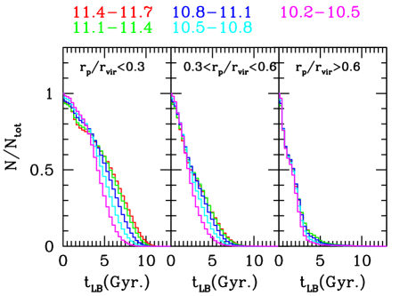
Figure 7: Cumulative distribution of (look-back) infall times $t_{LB}$ for satellites with $\log M_{\ast}/M_{\odot}>9$ in the semi-analytic galaxy catalogue. Colored curves distinguish our five primary stellar mass bins as labeled. We show three different ranges of projected radius: $r_{p}<0.3r_{\rm vir}$ (left), $0.3<r_{p}/r_{\rm vir}<0.6$ (middle) and $r_{p}>0.6r_{\rm vir}$ (right). Satellites in the inner regions typically fell in earlier than those in the outskirts by $\sim 2-3$ Gyr. This is consistent with the inside-out assembly of the halo and its satellite population, which is thus detected also in projection. About half of the satellites close to primaries with $M_{*}^{\rm pri}<11.1$ fell in more than 5 Gyr ago. Since Fig. 5 shows that the satellite population around low-mass SDSS primaries is dominated by blue objects, this suggests that the timescale for quenching star formation in satellites is at least $\sim 5$ Gyrs for such primaries.

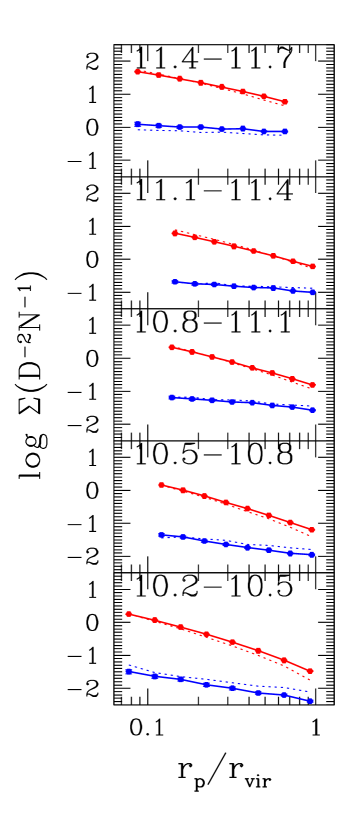
Figure 8: The effects of background cosmology on satellite profiles. Dotted/solid lines show the same physical model but for two different sets of cosmological parameters, WMAP-1 (G11) and WMAP-7 (G13), respectively. The impact of cosmology is apparently quite small.

3.4 Satellite number density profiles: comparison with previous work

A number of recent studies have examined the distribution of satellites in hybrid samples from spectroscopic + photometric catalogues using methods similar to our own (Lares et al., 2011; Guo et al., 2012; Nierenberg et al., 2011, 2012; Tal et al., 2012; Jiang et al., 2012; Guo et al., 2014). Most of them agree with us in finding the abundance of satellites to depend strongly on primary stellar mass (see also PaperI). However, in several cases the detailed trends we find with primary and satellite properties do not all agree with those published previously. For instance, the very weak dependence of the shape of satellite profiles on primary colour and satellite mass agrees well with Nierenberg et al.(2012), Wang et al. (2011) and Jiang et al. (2012) but is contrary to some of those in Tal et al. (2012), Watson et al. (2012) and Guo et al. (2014) who find bright satellites to be more radially concentrated. Our results are also in partial disagreement with Guo et al. (2012), who found the radial distribution of bright satellites to be less radially concentrated.

Some of these discrepancies can be explained by differences in sample definition. Our selection of isolated primaries discards all galaxy systems where the difference of $r$-band magnitude between the central object and the satellites is smaller than 1. This makes the comparison of our results with those found in groups and clusters more difficult to interpret. However, comparisons with Guo et al. (2012) are more interesting since their analysis uses similar selection criteria to our own and is also applied to objects in the SDSS/DR7 and DR8 catalogues.

The approaches to quantifying satellite radial distributions differ between our work and Guo et al. (2012): we use abundance matching arguments to infer the expected mean distribution of dark matter around our primary samples, and we compare this with the mean number density profiles we find for satellites, whereas Guo et al. fit NFW profiles directly to their estimated satellite distributions without reference to expectations for the host dark matter halos. The shapes of the number density profiles they measure for satellites of different luminosity agree for $r_{p}>0.12r_{\mathrm{vir}}$, but differ at smaller radii (see their Figure 6). The variations in the inner profiles are thus not totally unexpected, given the different choices and cuts applied to each sample. Here, we assume a fixed projected radius cut for all primaries in a given mass bin (see Table LABEL:tbl:primaries) whereas Guo et al. (2012) deal with the inner regions by excluding annuli that are within 1.5 times the Petrosian radius of the primary galaxy. This is typically a smaller radius than the cut we impose. For example, the luminosity range of primaries in Guo et al. (2012) corresponds roughly to the second most massive primary stellar mass bin in our analysis, for which we use $r_{\rm in}=50~{}{\rm kpc}\approx 0.12r_{\mathrm{vir}}$ (see Table LABEL:tbl:primaries), while the mean inner cut of Guo et al. (2012) is $r_{\rm in}=$23kpc and differs from galaxy to galaxy. On scales smaller than $0.1r_{\mathrm{vir}}$ systematics caused by proximity to the primary image are argued to be important by both Tal et al. (2012) and Watson et al. (2012), whereas no photometric corrections are made by Guo et al. (2012), which perhaps accounts for the different conclusions about inner profiles in these three studies. We chose such a more conservative inner radius cut because we have tested that satellite profiles at these radii are sensitive to photometric systematics (see the Appendix of paper I for more details). We exclude these radii from our analysis specifically to avoid the need to correct for such effects.

4 Treatment of environmental effects in semi-analytical catalogues

The serious discrepancy between satellite colours in the SDSS and in our semi-analytic catalogue clearly reflects an overestimation of environmental effects in the simulation. Once a simulated galaxy becomes a satellite, i.e. crosses the virial radius of a larger system, its external and internal gas reservoirs are reduced through tidal and ram-pressure stripping, with no further replenishment through cosmological infall. The reduction in fuel for star formation then causes satellites to form fewer stars and to redden compared to similar objects in the field. Studies by Guo et al. (2011) of colour-dependent autocorrelation functions in their model already revealed excess clustering of red galaxies on scales below $\sim 1$ Mpc. Our analysis of satellite properties allows a cleaner interpretation, tracing back the origin of the problem to an incorrect treatment of star formation for objects that orbit within a larger host halo. This problem with the G11 model was already clearly identified in the study of satellite colours in galaxy groups and clusters by Weinmann et al. (2010). These authors showed that although discrepancies were clearly smaller in G11 than in the earlier model studied by Weinmann et al. (2010), environmental effects were still too strong in lower mass systems.

We use the distribution of time since infall for simulated satellites to gain intuition on the appropriate timescale for suppression of star formation once a galaxy becomes a satellite. Fig. 7 shows the cumulative distribution of time since infall for satellites more massive than $\log M_{\ast}/M_{\odot}=9$. Time since infall $t_{\rm LB}$ is here defined as the time since the satellite last crossed the virial radius of its host halo. We group the satellites in our mock sample into three bins of projected radius normalized to the virial radius: from left to right these are $r_{p}<0.3r_{\rm vir}$, $0.3<r_{p}/r_{\rm vir}<0.6$ and $r_{p}>0.6r_{\rm vir}$. This allows us to see the dependence of infall time on distance to the host (Gao et al., 2004), or equivalently on binding energy (Rocha et al., 2012). Different colours indicate results for primaries in the five stellar mass bins defined above. Note that we only consider “true” satellites, defined as objects with 3D positions within the virial radius of each host halo, when we make this plot, although we bin as a function of projected radius to enable more direct comparison with observed systems.

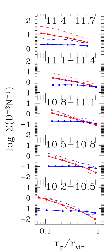
Figure 9: Prediction from an updated semi-analytic model (from Henriques et al. (2014, in prep.)) which, relative to the G11 model, has delayed reincorporation of gas ejected by supernovae, a lower star formation threshold, and no ram-pressure stripping in galaxy groups. The fraction of blue satellites (thick solid lines) is increased significantly, but the profiles remain flatter than those observed in SDSS (the thin dashed curves).

As expected, satellites in the inner regions typically have a longer time since infall than those at large radii, consistent with inside-out growth of the satellite population. Interestingly, we find that the time since infall is also typically longer in more massive halos. This is surprising, because dark matter concentrations and formation redshifts are typically lower for more massive halos. The trend we see is in part due to the fact that our isolated primaries are usually the central galaxies of fossil groups (galaxy groups with a large magnitude difference between the first and second brightest galaxies) and these assemble earlier than typical groups of their mass. The second brightest companions in our mock catalogue are typically 1.9, 2.4, 2.8, 2.8 and 2.5 magnitudes fainter in r-band than their primaries in the most- to least- massive stellar mass bin, respectively.

Fig. 7 shows that around isolated galaxies similar in mass to the Milky Way (the blue curves), half of all satellites that today have $r_{p}<0.3r_{\rm vir}$ first fell within the virial radius of the primary more than 5 Gyr ago, whereas for satellites with $r_{p}>0.6r_{\rm vir}$ the median time since infall is $\sim 2~{}{\rm Gyr}$. Fig. 5 and 6 show that most observed satellites of primaries with $\log M_{*}/M_{\odot}<11.1$ are blue, even at small radii, so the timescale for shutting-off star formation apparently needs to be at least 5 Gyr in such systems. For comparison, in the G11 model analyzed here, the mean time since infall for blue satellites of primaries with $\log M_{*}/M_{\odot}=11.1$ is only $\sim 0.9~{}{\rm Gyr}$.

If satellites in the G11 model redden too quickly compared to observation, could overly early collapse and halo assembly (due to an overly large $\sigma_{8}$ value) be responsible? We show in Fig. 8 the effect of cosmology on satellite profiles split by colour. Thick solid lines correspond to the Guo et al. (2013) model (G13), which is the same as G11 except that it corrects the cosmological parameters to be consistent with WMAP7. The differences from the original G11 model (the thin dotted lines) are small, indicating that the assumed background cosmology has little effect on the properties of satellites and thus cannot explain the discrepancy between the semi-analytic model and the SDSS data.

We take a closer look at the impact of different physical assumptions on the predicted profiles of red and blue satellites by analyzing predictions from an updated model specifically targeted at improving the treatment of satellite and low-mass galaxies. This model (Henriques et al. 2014, in prep) is based on G13 and adopts most of its physical prescriptions. An important modification is an increase in the timescale for reincorporation of material ejected to large radius by supernova explosions, particularly in low-mass systems and early times. This follows Henriques et al. (2013) and extends star formation to later times in low-mass galaxies. It has a large impact on the properties of central galaxies but the strong environmental effects in G11/G13 prevent it from substantially increasing the number of blue satellites.

To address this problem the updated model also reduces the threshold for star formation and removes the effects of ram-pressure stripping in galaxy groups. (Tidal stripping is assumed to act in groups of all masses, whereas ram-pressure effects are eliminated for group masses $M_{\rm{vir}}<10^{14}\hbox{$\rm\,M_{\odot}$}$.) These changes cause satellites in low-mass groups to retain their extended gas reservoirs for longer, and to convert more of their cold gas into stars. Together these modifications ensure that the bulk of low-mass satellites remains blue at later times. This model also updates the cosmological parameters to be consistent with PLANCK results, and modifies the scaling of the AGN radio-mode feedback to improve the properties of high-mass galaxies. These last two changes have negligible impact on the properties analyzed here.

Fig. 9 shows the distribution of red and blue satellites in the updated model (thick solid lines). Observations from SDSS are indicated by thin dashed lines. The new recipes produce a significant increase in the number of blue satellites around primaries of all masses. As a result, the normalization of the predicted blue population gets closer to observations. However, the profile shape for this blue population is only similar to that observed for the two most massive primary bins. Profiles are still significantly shallower than observed for low-mass primaries.

These results, together with an extensive series of tests in which we have arbitrarily suppressed individual environmental effects (not shown here for brevity) seem to indicate that straightforward modification of standard environmental effects cannot lead to a satellite population which remains predominantly blue at small separations. A possible solution might involve the enhancement of star formation in satellites near halo centre, perhaps as a result of tidal effects induced by the primary. There is some direct observational evidence that star formation can indeed be triggered by close tidal interactions (e.g., Lambas et al., 2003; Li et al., 2008; Ellison et al., 2008), and starbursts which may be tidally induced have been detected in the nuclei of S0 galaxies in the Fornax and Virgo clusters by Johnston et al. (2012, 2013), showing that star formation can take place in the bulge of these galaxies even as their disks redden with time. Furthermore, Ebeling et al. (2014) used high-resolution HST images to uncover evidence of shock-induced star formation in cluster galaxies undergoing ram-pressure stripping. Such environmental enhancement of star formation may counteract quenching processes to keep the fraction of star-forming satellites high even at small distances from lower mass primaries.

5 Conclusion and Discussion

We study the mean number density profiles of satellites around isolated primary galaxies selected from the spectroscopic catalogue of SDSS/DR7. We select satellites from the full photometric catalogue of SDSS/DR8, correcting statistically for contamination by unrelated foreground and background galaxies. Our sample contains about 41,000 isolated primaries with $\sim 7,000,000$ photometric companions (including background) projected within 500 kpc. We explore the dependence of these profiles on the stellar mass and colour of both primaries and satellites. Our results can be summarized as follows:

• The radial distribution of satellites depends on primary stellar mass. Satellites around massive primaries $\rm\log M_{*}/M_{\odot}>11.1$ have slightly shallower profiles than are predicted for the dark matter in their host halos, whereas for less massive primaries $10.2<\log M_{*}/M_{\odot}<11.1$ satellites follow quite closely the predicted dark matter profiles.

• We find the shape of satellite number density profiles to depend at most weakly on satellite stellar mass.

• Red primaries have more satellites than blue primaries of the same stellar mass, at least for $\log M_{*}/M_{\odot}>10.8$.

• Observed satellite number density profiles depend on satellite colour and behave differently for high- and low-mass primaries. For primaries with $\log M_{*}/M_{\odot}<11.1$, the blue and red populations have profiles of similar shape, consistent in both cases with that predicted for the dark matter distribution. Blue satellites dominate at all radii. Around more massive primaries ($\log M_{*}/M_{\odot}>11.1$) the blue population has a shallower profile and is subdominant at all radii.

We compare these observational results with satellite samples selected from the galaxy population simulation of Guo et al. (2011). The number density profiles of the whole satellite population always parallel the dark matter profile of the host halo, regardless of primary mass; this disagrees with the SDSS result for massive primaries. This may reflect the need for more efficient tidal disruption of satellites in the model. Satellite colours remain the most important challenge to these theoretical models, however. In the model the fraction of blue satellites is too small, particularly around low-mass primaries, and the few remaining blue satellites have an almost flat radial profile, in clear disagreement with the observations.

Given that observed satellites of low-mass primaries are predominantly blue at all projected radii, the distributions of time since infall that we find for simulated satellites imply that real satellites can remain actively star-forming as much as 5 Gyr after they have fallen into their current host halo, even when their orbit takes them into its inner regions. This seems qualitatively consistent with earlier work reporting that the decline of star formation in satellites occurs over extended periods of time (e.g. Wang et al., 2007; Weinmann et al., 2009; Wetzel et al., 2013; Trinh et al., 2013; Wheeler et al., 2014). The significantly shorter timescales implied by our model ($\sim 0.9$ Gyr) are responsible for its overabundance of red satellites. This indicates that the environmental suppression of star formation is overestimated by the model, particularly around low-mass primaries, and perhaps that the environmental stimulation of star formation needs to be included.

Indeed, from a series of experiments with differing treatments of environmental processes, we find that although the combined effect of suppressing ram-pressure stripping in low-mass halos ($M_{\mathrm{vir}}<10^{14}M_{\odot}$) and decreasing the density threshold for star formation can bring the overall blue fraction into agreement with SDSS, the shape of the blue satellite profile remains much flatter than observed. The fact that SDSS satellites are still predominantly blue even a few tens of kpc from low-mass primaries, suggests that processes which enhance star formation during close encounters need to be introduced into the models. Progress in this area will require a better understanding of tidally or shock-induced star formation, as well as observational studies which resolve the structure of star-forming regions in typical satellite galaxies.

Appendix A Projection effects in a light-cone and the local environment of isolated galaxies

Throughout our paper we have compared rectilinear projections of snapshots of the Millennium and Millennium-II simulations with observations from SDSS. Although most projection effects are taken care of in a realistic way in these mock galaxy samples (redshifts are computed using the line-of-sight distance within the box together with peculiar velocities) there are several factors affecting the SDSS data that are not properly represented. Among these, effects due to the fixed flux limit of a real survey and the K-corrections needed to obtain rest-frame magnitudes, fiber-fiber collision effects which make it difficult to obtain redshifts for close galaxy pairs, and the effects of the survey geometry stand out as possible sources of concern for our analysis. To address these issues, we have paralleled the analysis presented in the main body of our paper with studies of satellite profiles obtained from a light-cone galaxy catalogue taken from Henriques et al. (2012) . This light-cone is generated from the same Millennium-based galaxy population simulation as our other model catalogues, but properly includes evolutionary and band-pass shifting effects, as well as the flux limits of the survey, a simplified model for the effects of fiber-fiber collision, and the geometry of the SDSS mask. The selection for primaries and satellites can be applied to this light-cone catalogue in exactly the same way as to the observed SDSS sample.

Overall, we find good agreement between our original mock catalogue and that generated from the light-cone. We illustrate this by showing the projected number density profiles of satellites split according to primary colour from the light-cone sample in Fig. 10. Panels indicate different primary stellar mass bins, with the $\log M_{*}/M_{\odot}$ ranges quoted at the top left of each box. As before, orange and light-blue curves correspond to satellites of red and blue primaries, respectively (colour cuts for each primary stellar mass bin are as quoted in Table 1). This figure should be compared with the right column of Fig. 4. To guide the eye the black dashed lines in Fig. 10 are exactly those in the right column of Fig. 4. Agreement between the two samples is generally good, but for low-mass primaries, particularly blue ones, satellite profiles tend to fall off more rapidly at large radii than for the dark matter (black dashed lines). This effect is only marginally detected but appears to reflect a bias in the light-cone catalogue, since satellite profiles in 3D (Fig. 1) and projected directly from the box (right column Fig. 4) do not show such a steepening.

The probable source of this effect is an over-estimation of the background subtraction in our light-cone samples (both observational and simulated). The isolation criteria for primaries used in this paper and also in Paper I is quite strict, and as a result objects that fulfill it are significantly biased towards low density environments. Since our satellite profiles are estimated by subtracting the average projected number counts from the full catalogue, we over-correct for background at about the $\sim 1\%$ level. Although this is not a large effect in the satellite population as a whole, it becomes noticeable when the signal is weak, i.e. at large distances from low-mass primaries.

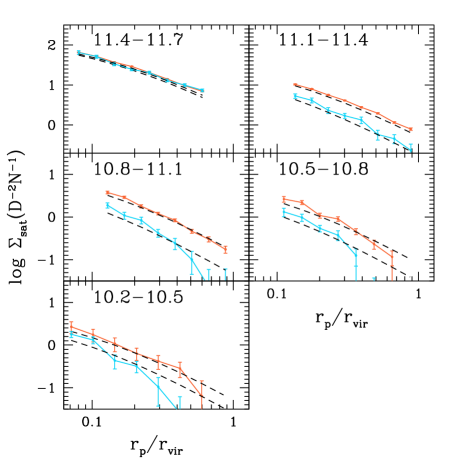
Figure 10: Same as Fig. 4 but for a simulated light-cone that mimics observational effects in the SDSS (see Henriques et al. 2012). The black dashed curves reproduce those in the right column of Fig. 4. There is a good agreement between the results from the light-cone and from the mock catalogue generated by rectilinear projection of a simulation snapshot. The steep decline of satellite profiles at large radii around blue low-mass primaries appears to reflect a bias in the environment of our primaries (see the text for more details).

We explore the local environment of isolated galaxies further in Fig.11, where we have selected primary galaxies from SDSS with more relaxed isolation criteria, increasing the primary sample by $\sim 40\%$ (primaries are still required to be the brightest galaxy within 1 Mpc and the line-of-sight velocity criterion is unchanged, but the stricter isolation criterion within 500 kpc is eliminated, see Planck Collaboration et al. (2013)). Thin dashed curves in Fig. 11 reproduce those in the left column of Fig. 4. The more relaxed isolation criteria translate into significantly shallower satellite profiles at large radii than those we obtained in Sec. 3.2 (the slope differences are significant only for $r>0.5r_{\rm vir}$). We have checked that this excess is due to the inclusion of a larger fraction of primaries that are not central galaxies of their FoF halo, with the consequences for the satellite profiles discussed in Sec. 3.2. Interestingly, the mean dark matter profiles in the simulation for this new primary sample show a similar excess at large radius, further evidence for our claim that satellites do indeed trace the underlying dark matter distribution very well, at least in the simulation. We also notice slightly higher normalizations for the inner satellite profiles in this new sample compared to Fig. 4. Primaries with relatively bright companions have more faint satellites than those which do not, an effect that we traced back to their having slightly more massive halos.

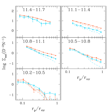
Figure 11: Satellite profiles for red and blue primary galaxies selected from SDSS with less strict isolation criteria (see the text for details). Thick orange and light-blue curves correspond to satellites of red and blue primaries. The thin dashed orange and light-blue curves reproduce those in the left column of Fig. 4. The outer profiles of low-mass primaries become shallower with less strict isolation.

References

- Abazajian et al. (2009) Abazajian K. N., Adelman-McCarthy J. K., Agüeros M. A., Allam S. S., Allende Prieto C., An D., Anderson K. S. J., Anderson S. F., Annis J., Bahcall N. A., et al. 2009, ApJS, 182, 543
- Aihara et al. (2011) Aihara H., et al., 2011, ApJS, 193, 29
- Blanton & Roweis (2007) Blanton M. R., Roweis S., 2007, AJ, 133, 734
- Blanton et al. (2005) Blanton M. R., Schlegel D. J., Strauss M. A., Brinkmann J., Finkbeiner D., Fukugita M., Gunn J. E., Hogg D. W., Ivezić Ž., Knapp G. R., Lupton R. H., Munn J. A., Schneider D. P., Tegmark M., Zehavi I., 2005, AJ, 129, 2562
- Bower et al. (2006) Bower R. G., Benson A. J., Malbon R., Helly J. C., Frenk C. S., Baugh C. M., Cole S., Lacey C. G., 2006, MNRAS, 370, 645
- Boylan-Kolchin et al. (2009) Boylan-Kolchin M., Springel V., White S. D. M., Jenkins A., Lemson G., 2009, MNRAS, 398, 1150
- Budzynski et al. (2012) Budzynski J. M., Koposov S. E., McCarthy I. G., McGee S. L., Belokurov V., 2012, MNRAS, 423, 104
- Chabrier (2003) Chabrier G., 2003, ApJL, 586, L133
- Chen (2008) Chen J., 2008, A&A, 484, 347
- Chen et al. (2006) Chen J., Kravtsov A. V., Prada F., Sheldon E. S., Klypin A. A., Blanton M. R., Brinkmann J., Thakar A. R., 2006, ApJ, 647, 86
- Coil et al. (2008) Coil A. L., Newman J. A., Croton D., Cooper M. C., Davis M., Faber S. M., Gerke B. F., Koo D. C., Padmanabhan N., Wechsler R. H., Weiner B. J., 2008, ApJ, 672, 153
- Colless et al. (2001) Colless M., Dalton G., Maddox S., Sutherland W., Norberg P., Cole S., Bland-Hawthorn J., Bridges 2001, MNRAS, 328, 1039
- Conroy et al. (2007) Conroy C., Wechsler R. H., Kravtsov A. V., 2007, ApJ, 668, 826
- Contini et al. (2014) Contini E., De Lucia G., Villalobos Á., Borgani S., 2014, MNRAS, 437, 3787
- Croton et al. (2006) Croton D. J., Springel V., White S. D. M., De Lucia G., Frenk C. S., Gao L., Jenkins A., Kauffmann G., Navarro J. F., Yoshida N., 2006, MNRAS, 365, 11
- Cunha et al. (2009) Cunha C. E., Lima M., Oyaizu H., Frieman J., Lin H., 2009, MNRAS, 396, 2379
- Ebeling et al. (2014) Ebeling H., Stephenson L. N., Edge A. C., 2014, ApJL, 781, L40
- Ellison et al. (2008) Ellison S. L., Patton D. R., Simard L., McConnachie A. W., 2008, AJ, 135, 1877
- Font et al. (2008) Font A. S., Bower R. G., McCarthy I. G., Benson A. J., Frenk C. S., Helly J. C., Lacey C. G., Baugh C. M., Cole S., 2008, MNRAS, 389, 1619
- Gao et al. (2004) Gao L., De Lucia G., White S. D. M., Jenkins A., 2004, MNRAS, 352, L1
- Gao et al. (2011) Gao L., Frenk C. S., Boylan-Kolchin M., Jenkins A., Springel V., White S. D. M., 2011, MNRAS, 410, 2309
- Gao et al. (2008) Gao L., Navarro J. F., Cole S., Frenk C. S., White S. D. M., Springel V., Jenkins A., Neto A. F., 2008, MNRAS, 387, 536
- Gao et al. (2004) Gao L., White S. D. M., Jenkins A., Stoehr F., Springel V., 2004, MNRAS, 355, 819
- Guo et al. (2014) Guo H., Zheng Z., Zehavi I., Xu H., Eisenstein D. J., Weinberg D. H., Bahcall N. A., Berlind A. A., Comparat J., McBride C. K., Ross A. J., Schneider D. P., Skibba R. A., Swanson M. E. C., Tinker J. L., Tojeiro R., Wake D. A., 2014, ArXiv e-prints
- Guo et al. (2012) Guo Q., Cole S., Eke V., Frenk C., 2012, MNRAS, 427, 428
- Guo et al. (2013) Guo Q., Cole S., Eke V., Frenk C., Helly J., 2013, ArXiv e-prints
- Guo & White (2014) Guo Q., White S., 2014, MNRAS, 437, 3228
- Guo et al. (2013) Guo Q., White S., Angulo R. E., Henriques B., Lemson G., Boylan-Kolchin M., Thomas P., Short C., 2013, MNRAS, 428, 1351
- Guo et al. (2011) Guo Q., White S., Boylan-Kolchin M., De Lucia G., Kauffmann G., Lemson G., Li C., Springel V., Weinmann S., 2011, MNRAS, 413, 101
- Henriques et al. (2012) Henriques B. M. B., White S. D. M., Lemson G., Thomas P. A., Guo Q., Marleau G.-D., Overzier R. A., 2012, MNRAS, 421, 2904
- Henriques et al. (2013) Henriques B. M. B., White S. D. M., Thomas P. A., Angulo R. E., Guo Q., Lemson G., Springel V., 2013, MNRAS, 431, 3373
- Holmberg (1969) Holmberg E., 1969, Arkiv for Astronomi, 5, 305
- Jiang et al. (2012) Jiang C. Y., Jing Y. P., Li C., 2012, ApJ, 760, 16
- Johnston et al. (2012) Johnston E. J., Aragón-Salamanca A., Merrifield M. R., Bedregal A. G., 2012, MNRAS, 422, 2590
- Johnston et al. (2013) Johnston E. J., Aragon-Salamanca A., Merrifield M. R., Bedregal A. G., 2013, ArXiv e-prints
- Kravtsov et al. (2004) Kravtsov A. V., Gnedin O. Y., Klypin A. A., 2004, ApJ, 609, 482
- Lambas et al. (2003) Lambas D. G., Tissera P. B., Alonso M. S., Coldwell G., 2003, MNRAS, 346, 1189
- Lares et al. (2011) Lares M., Lambas D. G., Domínguez M. J., 2011, AJ, 142, 13
- Li et al. (2008) Li C., Kauffmann G., Heckman T. M., Jing Y. P., White S. D. M., 2008, MNRAS, 385, 1903
- Li et al. (2006) Li C., Kauffmann G., Jing Y. P., White S. D. M., Börner G., Cheng F. Z., 2006, MNRAS, 368, 21
- Lorrimer et al. (1994) Lorrimer S. J., Frenk C. S., Smith R. M., White S. D. M., Zaritsky D., 1994, MNRAS, 269, 696
- Mandelbaum et al. (2006) Mandelbaum R., Hirata C. M., Broderick T., Seljak U., Brinkmann J., 2006, MNRAS, 370, 1008
- Moore et al. (1999) Moore B., Ghigna S., Governato F., Lake G., Quinn T., Stadel J., Tozzi P., 1999, ApJL, 524, L19
- Moster et al. (2010) Moster B. P., Somerville R. S., Maulbetsch C., van den Bosch F. C., Macciò A. V., Naab T., Oser L., 2010, ApJ, 710, 903
- Nagai & Kravtsov (2005) Nagai D., Kravtsov A. V., 2005, ApJ, 618, 557
- Navarro et al. (1996) Navarro J. F., Frenk C. S., White S. D. M., 1996, ApJ, 462, 563
- Navarro et al. (1997) Navarro J. F., Frenk C. S., White S. D. M., 1997, ApJ, 490, 493
- Nierenberg et al. (2011) Nierenberg A. M., Auger M. W., Treu T., Marshall P. J., Fassnacht C. D., 2011, ApJ, 731, 44
- Nierenberg et al. (2012) Nierenberg A. M., Auger M. W., Treu T., Marshall P. J., Fassnacht C. D., Busha M. T., 2012, ApJ, 752, 99
- Planck Collaboration et al. (2013) Planck Collaboration Ade P. A. R., Aghanim N., Arnaud M., Ashdown M., Atrio-Barandela F., Aumont J., Baccigalupi C., Balbi A., Banday A. J., et al. 2013, AA, 557, A52
- Prescott et al. (2011) Prescott M., et al., 2011, MNRAS, 417, 1374
- Presotto et al. (2014) Presotto V., Girardi M., Nonino M., Mercurio A., Grillo C., Rosati P., Biviano A., Annunziatella M., 2014, ArXiv e-prints
- Rocha et al. (2012) Rocha M., Peter A. H. G., Bullock J., 2012, MNRAS, 425, 231
- Sales & Lambas (2005) Sales L., Lambas D. G., 2005, MNRAS, 356, 1045
- Sales et al. (2007) Sales L. V., Navarro J. F., Lambas D. G., White S. D. M., Croton D. J., 2007, MNRAS, 382, 1901
- Springel et al. (2008) Springel V., Wang J., Vogelsberger M., Ludlow A., Jenkins A., Helmi A., Navarro J. F., Frenk C. S., White S. D. M., 2008, MNRAS, 391, 1685
- Springel et al. (2005) Springel V., White S. D. M., Jenkins A., Frenk C. S., Yoshida N., Gao L., Navarro J., Thacker R., Croton D., Helly J., Peacock J. A., Cole S., Thomas P., Couchman H., Evrard A., Colberg J., Pearce F., 2005, Nature, 435, 629
- Springel et al. (2001) Springel V., White S. D. M., Tormen G., Kauffmann G., 2001, MNRAS, 328, 726
- Tal et al. (2012) Tal T., Wake D. A., van Dokkum P. G., 2012, ApJL, 751, L5
- Trinh et al. (2013) Trinh C. Q., Barton E. J., Bullock J. S., Cooper M. C., Zentner A. R., Wechsler R. H., 2013, MNRAS, 436, 635
- van den Bosch et al. (2008) van den Bosch F. C., Aquino D., Yang X., Mo H. J., Pasquali A., McIntosh D. H., Weinmann S. M., Kang X., 2008, MNRAS, 387, 79
- van den Bosch et al. (2005) van den Bosch F. C., Yang X., Mo H. J., Norberg P., 2005, MNRAS, 356, 1233
- Wang et al. (2008) Wang J., De Lucia G., Kitzbichler M. G., White S. D. M., 2008, MNRAS, 384, 1301
- Wang et al. (2012) Wang J., Frenk C. S., Navarro J. F., Gao L., Sawala T., 2012, MNRAS, p. 3369
- Wang et al. (2007) Wang L., Li C., Kauffmann G., De Lucia G., 2007, MNRAS, 377, 1419
- Wang et al. (2011) Wang W., Jing Y. P., Li C., Okumura T., Han J., 2011, ApJ, 734, 88
- Wang & White (2012) Wang W., White S. D. M., 2012, MNRAS, 424, 2574
- Watson et al. (2012) Watson D. F., Berlind A. A., McBride C. K., Hogg D. W., Jiang T., 2012, ApJ, 749, 83
- Weinmann et al. (2009) Weinmann S. M., Kauffmann G., van den Bosch F. C., Pasquali A., McIntosh D. H., Mo H., Yang X., Guo Y., 2009, MNRAS, 394, 1213
- Weinmann et al. (2010) Weinmann S. M., Kauffmann G., von der Linden A., De Lucia G., 2010, MNRAS, 406, 2249
- Weinmann et al. (2011) Weinmann S. M., Lisker T., Guo Q., Meyer H. T., Janz J., 2011, MNRAS, 416, 1197
- Weinmann et al. (2006) Weinmann S. M., van den Bosch F. C., Yang X., Mo H. J., 2006, MNRAS, 366, 2
- Wetzel et al. (2012) Wetzel A. R., Tinker J. L., Conroy C., 2012, MNRAS, 424, 232
- Wetzel et al. (2013) Wetzel A. R., Tinker J. L., Conroy C., van den Bosch F. C., 2013, MNRAS, 432, 336
- Wheeler et al. (2014) Wheeler C., Phillips J. I., Cooper M. C., Boylan-Kolchin M., Bullock J. S., 2014, ArXiv e-prints
- White & Rees (1978) White S. D. M., Rees M. J., 1978, MNRAS, 183, 341
- Wojtak & Mamon (2013) Wojtak R., Mamon G. A., 2013, MNRAS, 428, 2407
- Yang et al. (2009) Yang X., Mo H. J., van den Bosch F. C., 2009, ApJ, 693, 830
- York et al. (2000) York D. G., et al., 2000, AJ, 120, 1579
- Zehavi et al. (2011) Zehavi I., Zheng Z., Weinberg D. H., Blanton M. R., Bahcall N. A., Berlind A. A., Brinkmann J., Frieman J. A., Gunn J. E., Lupton R. H., Nichol R. C., Percival W. J., Schneider D. P., Skibba R. A., Strauss M. A., Tegmark M., York D. G., 2011, ApJ, 736, 59
- Zhao et al. (2009) Zhao D. H., Jing Y. P., Mo H. J., Börner G., 2009, ApJ, 707, 354