Rise of pairwise thermal entanglement for an alternating Ising and Heisenberg spin chain in an arbitrarily oriented magnetic field

Abstract

Typically two particles (spins) could be maximally entangled at zero temperature, and for a certain temperature the phenomenon of entanglement vanishes at the threshold temperature. For the Heisenberg coupled model or even the Ising model with a transverse magnetic field, one can observe some rise of entanglement even for a disentangled region at zero temperature. So we can understand this emergence of entanglement at finite temperature as being due to the mixing of some maximally entangled states with some other untangled states. Here, we present a simple one-dimensional Ising model with alternating Ising and Heisenberg spins in an arbitrarily oriented magnetic field, which can be mapped onto the classical Ising model with a magnetic field. This model does not show any evidence of entanglement at zero temperature, but surprisingly at finite temperature rise a pairwise thermal entanglement between two untangled spins at zero temperature, when an arbitrarily oriented magnetic field is applied. This effect is a purely magnetic field ,and the temperature dependence, as soon as the temperature increases, causes a small increase in concurrence achieving its maximum at around 0.1. Even for long-range entanglement, a weak concurrence still survives. There are also some real materials that could serve as candidates that would exhibit this effect, such as Dy(NO₃)(DMSO)₂Cu(opba)(DMSO)₂hagiwara-strecka .

Condensed matter researchers have long investigated the correlation function between parts of composite systems, thus it is relevant to study the quantum part of these correlations, which is called entanglement. Quantum entanglement is one of the most fascinating features of quantum theory due to its nonlocal property. Therefore, quantum entanglement has been the subject of many research in recent years as a potential resource for information processing and quantum computing.

Quantum entanglement , with its applications to quantum phase transitions of strongly correlated spin systems and its experimental implementation in optical lattices, was considered, in particular, for one-dimensional systems. Diverging entanglement length without quantum phase transition was found in localizable entanglement (LE) for VBSs, since the correlation length remains finitevestraete . This is a rather remarkable result regarding the entanglement properties of VBS quantum spin ground states. A theory for localizable entanglement was developed based on matrix product states coming from DMRG method and applied to VBS statespopp . In reference garcia , an experimental implementation was proposed for VBSs of spin-1 Heisenberg Hamiltonians and ladders, and a method was proposed to directly measure quantum observables that are not accessible in standard materials in condensed matter.

Recently, special attention has been focused on synthesizing Ising-Heisenberg chains, which are well represented as spin systems composed of Ising (classical) and Heisenberg (quantum) spinsvalverde08 ; ohanyan09 ; antonosyan09 ; canova09 ; rojas-ohanyan ; ana-roj ; strecka-jasc05 ; vanden10 ; sahoo12 . Ising-Heisenberg chains plays an important role in providing evidence for several novel and unexpected quantum states valverde08 ; ohanyan09 ; antonosyan09 ; canova09 ; rojas-ohanyan , such as thermal entanglement, fractional magnetization plateaus in the low-temperature magnetization process antonosyan09 ; canova09 ; rojas-ohanyan , and so on. Thus, real materials with experimental realizations of Ising-Heisenberg chains can be represented by the aforementioned theoretical findings, such as the magnetic behavior of a tetramer Ising-Heisenberg bond-alternating chain as a polymeric model Cu(3-Clpy)₂(N₃)₂ strecka-jasc05 . Another magnetic polymer is the dysprosium material [{(CuL)₂Dy}{Mo(CN)₈}] which can be represented experimentally through an Ising-Heisenberg chain as a [DyCuMoCu] infinite chainvanden10 ; bellucci , and the single chain magnet [{(H₂O)Fe(L)}{Nb(CN)₈}{Fe(L)}] sahoo12 was well described within the framework of the Ising-Heisenberg chains.

Here, we consider the alternating Ising and Heisenberg spin chain under arbitrarily oriented magnetic field, which nicely describes the 3d-4f bimetallic polymeric compound Dy(NO₃)(DMSO)₂Cu(opba)(DMSO)₂hagiwara-strecka , which provides an interesting experimental realization of the ferrimagnetic chain composed of two different but regularly alternating spin-1/2 magnetic ions Dy³⁺ and Cu²⁺ that are reasonably approximated by the notion of Ising and Heisenberg spins, respectively.

1. The alternating Ising and Heisenberg spin chain in an arbitrarily oriented magnetic field.

Let us consider the following Hamiltonian under an arbitrarily oriented magnetic field,

$$\mathcal{H}=-\sum_{i=1}^{N}\left((J\sigma_{i}^{z}+\frac{h_{1}}{2})(s_{i}+s_{i+1})+\boldsymbol{h}.\boldsymbol{\sigma}_{i}\right),$$ (1)

where $\boldsymbol{h}.\boldsymbol{\sigma}_{i}=h_{z}\sigma_{i}^{z}+h_{x}\sigma_{i}^{x}+h_{y}\sigma_{i}^{y}$, with $h_{x}=g_{x}h\sin(\phi)\cos(\theta)$, $h_{y}=g_{y}h\sin(\phi)\sin(\theta)$, $h_{z}=g_{z}h\cos(\phi)$ and $h_{1}=g_{1,z}h\cos(\phi)$, assuming $\theta\in[0,2\pi]$ and $\phi\in[0,\pi]$, and $\sigma^{\alpha}$ is the Pauli matrix for the Heisenberg spin, while $s$ corresponds to the Ising spin ($s=\pm 1)$. The exchange coupling parameter between $s$ and $\sigma^{z}$ spins is given by $J$.

Writing in matrix form, the Hamiltonian for the unit cell becomes

$$\mathcal{H}_{i,i+1}(\mu)=\left(\begin{array}[]{cc}-(J\mu+h_{z})-\frac{h_{1}\mu}{2}&-h_{x}+\hat{\imath}h_{y}\\ -h_{x}-\hat{\imath}h_{y}&(J\mu+h_{z})-\frac{h_{1}\mu}{2}\end{array}\right),$$ (2)

with $\mu=s_{i}+s_{i+1}$.

To use the decoration transformationstrecka pla ; JPA-11 , we need to diagonalize the Hamiltonian (2), whose eigenvalues are given by

$$\mathcal{E}_{i,i+1}(\mu)=-\frac{h_{1}}{2}\mu\pm A(\mu),$$ (3)

where $A(\mu)=\sqrt{(J\mu+h_{z})^{2}+h_{x}^{2}+h_{y}^{2}}$.

This model can be solved exactly through a decoration transformationstrecka pla ; JPA-11 and transfer matrix approachbaxter-book .

To compute all thermodynamic quantities, we need to calculate the Boltzmann factor given by

$$w(\mu) =\text{tr}_{\sigma}\left({\rm e}^{-\beta\mathcal{H}_{i,i+1}(\mu)}\right)=2{\rm e}^{\beta\mu\frac{h_{1}}{2}}\cosh(-\beta A(\mu)).$$ (4)

Once the Boltzmann factor is known, the transfer matrix can be expressed as follow

$$\boldsymbol{W}=\left(\begin{array}[]{cc}w(2)&w(0)\\ w(0)&w(-2)\end{array}\right).$$ (5)

Furthermore, the eigenvalues of the transfer matrix can be expressed by

$$\lambda_{\pm}=\frac{w(2)+w(-2)}{2}\pm\frac{B}{2},$$ (6)

with $B=\sqrt{(w(2)-w(-2))^{2}+4w(0)^{2}}$.

The corresponding non singular matrix that diagonalize the transfer matrix $\boldsymbol{T}$, becomes

$$\boldsymbol{V}=\left(\begin{array}[]{cc}b_{+}&b_{-}\\ 1&1\end{array}\right)\;\text{and}\;\boldsymbol{V}^{-1}=\tfrac{1}{b_{-}-b_{+}}\left(\begin{array}[]{cc}1&-b_{-}\\ -1&b_{+}\end{array}\right),$$ (7)

with $b_{\pm}=\frac{w(2)-w(-2)\pm B}{2w(0)}$.

2. The correlation function.

To perform the expectation value and correlation function, we need to perform the following quantity

$$w_{\alpha}(\mu)={\rm tr}_{\sigma}\left(\sigma_{i}^{\alpha}{\rm e}^{-\beta\mathcal{H}_{i,i+1}(\mu)}\right).$$ (8)

In fact, the trace of these quantities can be expressed easily as the derivative of the Boltzmann factor, $w_{\alpha}(\mu)=\frac{\partial w(\mu)}{\beta\partial h_{\alpha}},$ thus, each derivatives components becomes $w_{x}(\mu)=h_{x}\bar{w}(\mu)$, $w_{y}(\mu)=h_{y}\bar{w}(\mu)$ and $w_{z}(\mu)=(J\mu+h_{z})\bar{w}(\mu),$ where

$$\bar{w}(\mu)=\frac{2{\rm e}^{\beta\mu\frac{h_{1}}{2}}\sinh(-\beta A(\mu))}{A(\mu)}.$$ (9)

Thereafter, writing in matrix form, we have

$$\boldsymbol{W}_{\alpha}=\left(\begin{array}[]{cc}w_{\alpha}(2)&w_{\alpha}(0)\\ w_{\alpha}(0)&w_{\alpha}(-2)\end{array}\right).$$ (10)

The expectation value of $\sigma^{\alpha}$ is denoted by $\langle\sigma^{\alpha}\rangle$, thus in thermodynamic limit ($N\rightarrow\infty$) one can write as follow

$$\langle\sigma^{\alpha}\rangle=\frac{1}{\lambda_{+}}{\rm tr}\left[\boldsymbol{V}^{-1}\boldsymbol{W}_{\alpha}\boldsymbol{V}\left(\begin{array}[]{cc}1&0\\ 0&0\end{array}\right)\right],$$ (11)

defining $\boldsymbol{V}^{-1}\boldsymbol{W}_{\alpha}\boldsymbol{V}=\frac{1}{b_{+}-b_{-}}\widetilde{\boldsymbol{W}}_{\alpha}$, with $\widetilde{\boldsymbol{W}}_{\alpha}$ given by $\widetilde{\boldsymbol{W}}_{\alpha}=\left(\begin{array}[]{cc}\nu_{11}^{\alpha}&\nu_{12}^{\alpha}\\ \nu_{21}^{\alpha}&\nu_{22}^{\alpha}\end{array}\right)$, whose elements are

$$\nu_{11}^{\alpha}= b_{+}w_{\alpha}(2)+2w_{\alpha}(0)-b_{-}w_{\alpha}(-2),$$ (12)

$$\nu_{12}^{\alpha}= b_{-}w_{\alpha}(2)+(1-b_{-}^{2})w_{\alpha}(0)-b_{-}w_{\alpha}(-2),$$ (13)

$$\nu_{21}^{\alpha}= -b_{+}w_{\alpha}(2)-(1-b_{+}^{2})w_{\alpha}(0)+b_{+}w_{\alpha}(-2),$$ (14)

$$\nu_{22}^{\alpha}= -b_{-}w_{\alpha}(2)-2w_{\alpha}(0)+b_{+}w_{\alpha}(-2).$$ (15)

After taking the trace and assuming $b_{+}-b_{-}=\frac{B}{w(0)}$, the correlation function goes to

$$\langle\sigma^{\alpha}\rangle=\frac{w(0)}{B\lambda_{+}}\left(b_{+}w_{\alpha}(2)+2w_{\alpha}(0)-b_{-}w_{\alpha}(-2)\right).$$ (16)

Consequently, we define the following quantities

$$m_{0} =\frac{w(0)}{B\lambda_{+}}\left(b_{+}\bar{w}(2)+2\bar{w}(0)-b_{-}\bar{w}(-2)\right),$$ (17)

$$m_{1} =\frac{w(0)}{B\lambda_{+}}\left(b_{+}\bar{w}(2)+b_{-}\bar{w}(-2)\right),$$ (18)

thus, the expectation value of $\sigma^{\alpha}$ become

$$\langle\sigma^{x}\rangle=h_{x}m_{0},\;\langle\sigma^{y}\rangle=h_{y}m_{0},\;\langle\sigma^{z}\rangle=h_{z}m_{0}+2Jm_{1}.$$ (19)

It is worth noting that, the expectation value $\langle\sigma^{\alpha}\rangle$ can be expressed only in terms of the Boltzmann factor $w(\mu)$ and its derivative $w_{\alpha}(\mu)$, since, $b_{\pm}$ and $B$ were also defined in terms of the Boltzmann factor.

In a similar way, we can develop the correlation function in the thermodynamic limit,

$$\langle\sigma_{i}^{\alpha}\sigma_{i+r}^{\alpha^{\prime}}\rangle=\frac{w(0)^{2}}{B^{2}\lambda_{+}^{2}}{\rm tr}\left[\widetilde{\boldsymbol{W}}_{\alpha}\left(\begin{array}[]{cc}1&0\\ 0&q^{r-1}\end{array}\right)\widetilde{\boldsymbol{W}}_{\alpha^{\prime}}\left(\begin{array}[]{cc}1&0\\ 0&0\end{array}\right)\right],$$ (20)

where $q$ is the transfer matrix eigenvalues ratio $q=\frac{\lambda_{-}}{\lambda_{+}}$. After some algebraic manipulation, the correlation function becomes

$$\langle\sigma_{i}^{\alpha}\sigma_{i+r}^{\alpha^{\prime}}\rangle= \langle\sigma^{\alpha}\rangle\langle\sigma^{\alpha^{\prime}}\rangle+\left(\tfrac{w_{\alpha}(2)-w_{\alpha}(-2)-(b_{-}+b_{+})w_{\alpha}(0)}{(b_{+}-b_{-})\lambda_{+}}\right)\times$$

$$\left(\tfrac{w_{\alpha^{\prime}}(2)-w_{\alpha^{\prime}}(-2)-(b_{-}+b_{+})w_{\alpha^{\prime}}(0)}{(b_{+}-b_{-})\lambda_{+}}\right)q^{r-1}.$$ (21)

For a particular case when $\alpha^{\prime}=\alpha$, it is worth noting that all correlation function of the form $\langle\sigma_{i}^{\alpha}\sigma_{i+r}^{\alpha}\rangle$ are always positive. Using a convenient notation,

$$p_{0} =\frac{w(0)}{B\lambda_{+}}\left(\bar{w}(2)+(b_{+}+b_{-})\bar{w}(0)-\bar{w}(-2)\right),$$ (22)

$$p_{1} =\frac{w(0)}{B\lambda_{+}}\left(\bar{w}(2)+\bar{w}(-2)\right).$$ (23)

we will describe the correlation function as follow,

$$\langle\sigma_{i}^{x}\sigma_{i+r}^{x}\rangle= \langle\sigma^{x}\rangle^{2}+h_{x}^{2}p_{0}^{2}q^{r-1},$$ (24)

$$\langle\sigma_{i}^{y}\sigma_{i+r}^{y}\rangle= \langle\sigma^{y}\rangle^{2}+h_{y}^{2}p_{0}^{2}q^{r-1},$$ (25)

$$\langle\sigma_{i}^{x}\sigma_{i+r}^{y}\rangle= \langle\sigma^{x}\rangle\langle\sigma^{y}\rangle+h_{x}h_{y}p_{0}^{2}q^{r-1},$$ (26)

$$\langle\sigma_{i}^{z}\sigma_{i+r}^{z}\rangle= \langle\sigma^{z}\rangle^{2}+\left(p_{0}h_{z}+2Jp_{1}\right)^{2}q^{r-1}.$$ (27)

Once again, all correlation for Heisenberg spins can be expressed only in terms of the Boltzmann factor and its derivative.

3. Thermal entanglement.

Despite the system being untangled at zero temperature, it is of great relevance to discuss the entanglement at a non-zero temperature. Thus, we consider the quantum entanglement between a pair of Heisenberg spins in an arbitrarily oriented magnetic field.

As a measure of entanglement for two arbitrary mixed states of two qubits, we use the quantity called concurrencewooters , which was defined in terms of reduced density matrix $\rho$ of two mixed states,

$$\mathcal{C}(\rho)=\max\{{0,2\Lambda_{{\rm max}}-\text{{tr}}\sqrt{R}}\},$$ (28)

assuming $R=\rho\sigma^{y}\otimes\sigma^{y}\rho^{*}\sigma^{y}\otimes\sigma^{y},$ where $\Lambda_{{\rm max}}$ is the largest eigenvalue of the matrix $\sqrt{R}$, and $\rho^{*}$ represents the complex conjugate of matrix $\rho$, with $\sigma^{y}$ being the Pauli matrix.

For the case of an infinite chain, the reduced density operator elementsbukman could be expressed in terms of the correlation function between two entangled particlesamico , thus we have

$$\mathcal{C}_{r}(\theta,\phi)= \frac{1}{2}\max\left\{P_{r}^{xy}-\left|1-\langle\sigma_{i}^{z}\sigma_{i+r}^{z}\rangle^{2}\right|,0\right\}$$ (29)

where $P_{r}^{xy}=\sqrt{\left(\langle\sigma_{i}^{x}\sigma_{i+r}^{x}\rangle-\langle\sigma_{i}^{y}\sigma_{i+r}^{y}\rangle\right)^{2}+4\langle\sigma_{i}^{x}\sigma_{i+r}^{y}\rangle^{2}}$.

For the particular case when $g_{x}=g_{y}$, the concurrence becomes independent of $\theta$, and reduces to

$$\mathcal{C}_{r}(\phi)=\frac{1}{2}\max\left\{0,2\langle\sigma_{i}^{x}\sigma_{i+r}^{x}\rangle+\langle\sigma_{i}^{z}\sigma_{i+r}^{z}\rangle-1\right\}.$$ (30)

Using this result, we will illustrate the entangled region and how the concurrence behave. Alternatively, we can also obtain an equivalent result using the approach described in Ref spra .

Figure 1: (Color online) The arising of pairwise thermal entanglement (green region). (a) The concurrence $\mathcal{C}$ between the nearest Heisenberg spin $r=1$, as a function of the magnetic field $h/|J|$ and the polar angle $\phi$. (b) The concurrence $\mathcal{C}$ between the next-nearest Heisenberg spin $r=2$, as a function of the magnetic field $h/|J|$ and the polar angle $\phi$.

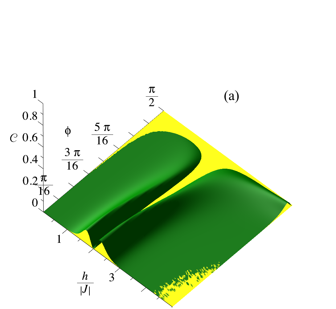
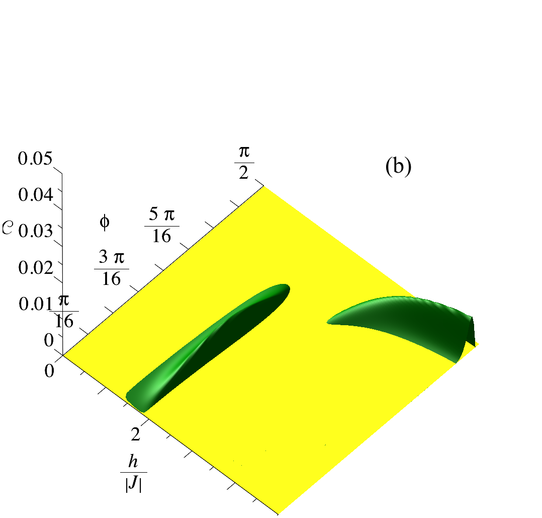
In figure 1, we illustrate the arising of pairwise thermal entanglement [green (gray) region], while the yellow region corresponds to the untangled region. By the use of concurrence, we display the intensity of entanglement, assuming the following gyromagnetic factors: $g_{x}=1.5$, $g_{z}=2.0$, and $g_{1z}=1.0$. We also choose the coupling parameter $J=-1.0$, while the temperature is assumed to be $T/|J|=0.3$. In figure 1(a), we illustrate the concurrence $\mathcal{C}$ as a function of magnetic field and polar angle $\phi$ for the nearest neighbor of the Heisenberg spin ($r=1$). But actually it means the second nearest neighbor, because there is one Ising spin between two Heisenberg spins. There is an entangled region for a relatively low magnetic field, $h/|J|\lesssim 2$, while for $h/|J|\gtrsim 2$ there is another entangled region. It is worth mentioning the dependence of the polar angle $\phi$. When a pure transverse magnetic field is applied to an alternating spin chain, this entanglement vanishes at $\phi=\frac{\pi}{2}$. Despite the fact that the transverse magnetic field ($\phi=\frac{\pi}{2}$) never generates concurrence for a high magnetic field, a relatively intense concurrence appears in the limit of $\phi\rightarrow\frac{\pi}{2}$, while for $\phi<\frac{\pi}{2}$ and a high magnetic field the concurrence vanishes. Similarly, figure 1(b) illustrates the concurrence $\mathcal{C}$ for the case of $r=2$ (next-nearest neighbor between Heisenberg spins). It should be noted that between this pair of Heisenberg spins, there are two Ising spins. So it is still possible to observe a weak concurrence around $\mathcal{C}\thickapprox 0.01$, however the entangled (green) region shrunk significantly. The entanglement for longer pair spins still appears for $r=3$ and $4$, with maximum concurrence $\mathcal{C}\thickapprox 0.001$, and for a tiny specific region, which is not illustrated here due to the irrelevant amount of concurrence.

Figure 2: (Color online) The arising of pairwise thermal entanglement (green region). (a) The concurrence $\mathcal{C}$ between nearest the Heisenberg spin $r=1$, as a function of the temperature $T/|J|$ and the polar angle $\phi$. (b) The concurrence $\mathcal{C}$ between the next-nearest Heisenberg spin $r=2$, as a function of the temperature $T/|J|$ and the polar angle $\phi$.

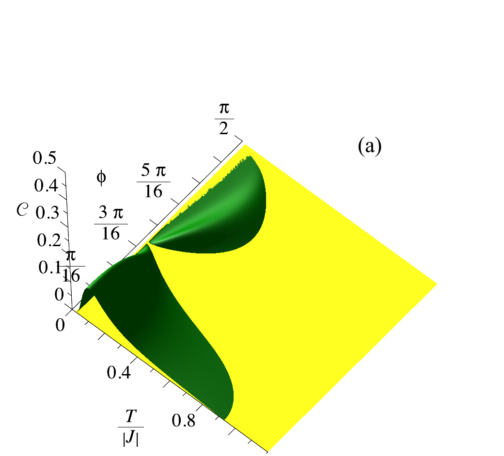
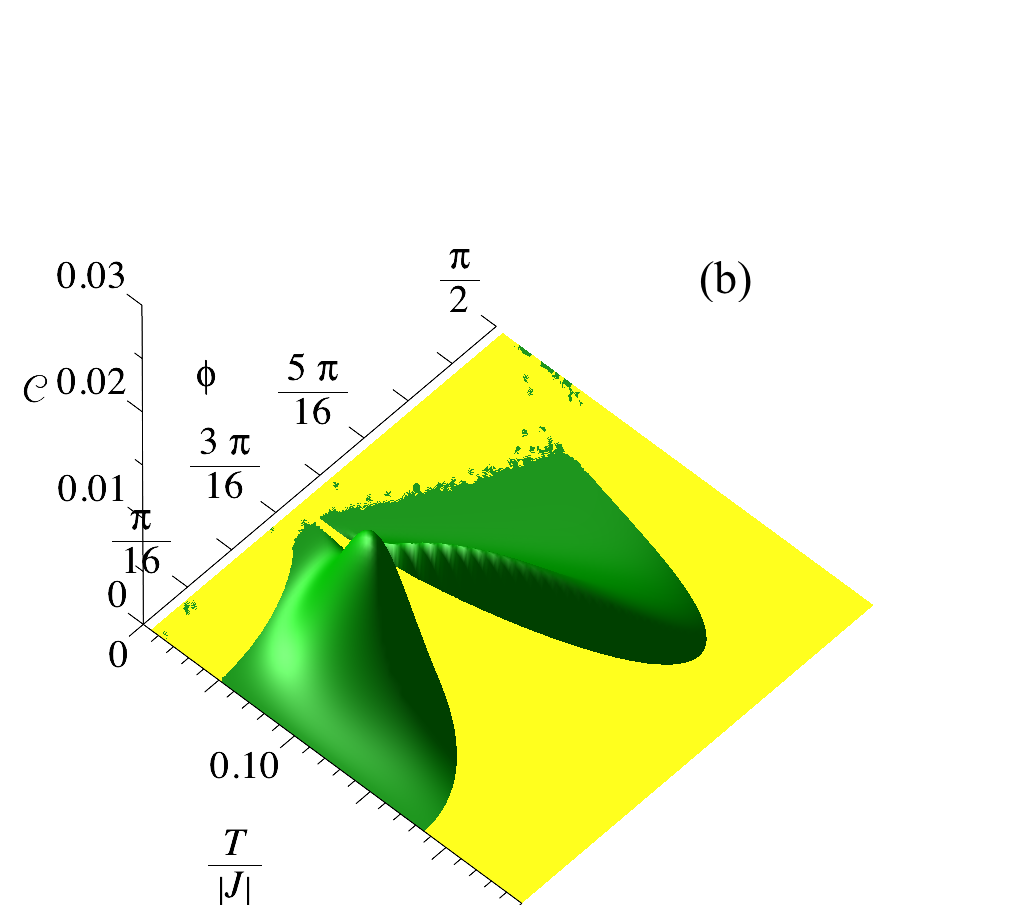
In figure 2(a) we illustrate the concurrence $\mathcal{C}$ as a function of temperature and polar angle $\phi$ for nearest neighbor of Heisenberg spin ($r=1$), for a fixed magnetic field $h/|J|=2.1$. There is a stronger entangled region for $0<\phi\lesssim\frac{3\pi}{16}$, while for $\frac{3\pi}{16}\lesssim\phi<\frac{\pi}{2}$, a weaker entangled region is observed, it is worth to notice the temperature dependence of concurrence disappear at the threshold temperature. Similarly, figure 2(b) also illustrates the concurrence $\mathcal{C}$ for the case of $r=2$.

4. Concurrence for powder samples.

Synthesized real materials are usually known as the single molecule magnets chainsvanden10 ; sahoo12 ; hagiwara-strecka , so it is natural to define the concurrence for the powder samples as an average of concurrence for powder samples. In what follows, we will discuss our theoretical results with measurements performed on powder samples of the crystalline compounds. Let $\theta$ and $\phi$ be azimuthal and polar angles of the magnetic field vector with respect to a molecular reference frame; thus the powder sample concurrence can be defined as a function of $\theta$ and $\phi$ ,

$$\mathcal{\bar{C}}_{r}=\frac{1}{4\pi}\int_{0}^{\pi}\int_{0}^{2\pi}\mathcal{C}_{r}(\theta,\phi)\sin(\phi){\rm d}\theta{\rm d}\phi.$$ (31)

For the case of $g_{x}=g_{y}$, the concurrence is independent of the angle $\theta$; thus we only need to integrate over the polar angle $\phi$. Hereafter, we observe the concurrence for the powder sample as a function of magnetic field and temperature.

Figure 3: (Color online) Concurrence as a function of temperature for a fixed value of magnetic field. (a) Nearest-neighbor concurrence $r=1$. (b) Next-nearest-neighbor concurrence $r=2$.

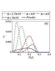
In figure 3(a) is illustrated the nearest-neighbor concurrence ($r=1$), assuming fixed values $h/|J|=1.7$ and $J=-1$. The black solid line corresponds to the powder sample concurrence given in eq.(31), while the dashed line corresponds to the concurrence for a fixed value of $\phi=\pi/8$, with the maximum concurrence $\mathcal{C}\approx 0.11$ at around $T/|J|\approx 0.4$. For other angles, the concurrence vanishes quickly, such as for the dashed-dotted line representing the concurrence for $\phi=\pi/4$, whose maximum occurs at $\mathcal{C}\approx 0.08$ and for $T/|J|\approx 0.5$. In contrast, figure 3(b) corresponds to the next-nearest-neighbor (NNN) pairwise concurrence ($r=2$), taking into account fixed values $h/|J|=2.0$ and $J=-1$. The black solid line represents to the powder sample concurrence, the dotted line corresponds to the concurrence for a fixed value of $\phi=2.7\pi/16$, the dashed-dotted line represents the concurrence for $\phi=\pi/8$, the long-dashed line corresponds to $\phi=\pi/4$, and finally the dashed line represents the concurrence for $\phi=5\pi/16$.

Figure 4: (Color online) Concurrence as a function of magnetic field for a fixed temperature. (a) Nearest-neighbor concurrence $r=1$. (b) Next-nearest-neighbor concurrence $r=2$.

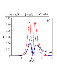
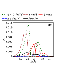
Furthermore, in figure 4 is illustrated the concurrence as a function of magnetic field for a fixed temperature and $J=-1$. In fig.4(a), we illustrate the concurrence for nearest-neighbor ($r=1$) and fixed temperature $T/|J|=0.3$. The black solid line corresponds to the powder sample concurrence given in eq.(31). While the dashed line corresponds to the concurrence for a fixed value of $\phi=\pi/8$, with maximum concurrence $\mathcal{C}\approx 0.11$ at around $h/|J|\approx 1.7$ and $h/|J|\approx 2.5$. For other angles, concurrence vanishes quickly, such as for the dashed-dotted line representing the concurrence for $\phi=\pi/4$, with a maximum at around $\mathcal{C}\approx 0.06$ and for an external magnetic field $h/|J|\approx 0.75$ and $h/|J|\approx 2.6$. The fig.4(b) corresponds to NNN pairwise concurrence $r=2$ and assuming $T/|J|=0.115$. The black solid line corresponds to powder sample concurrence, the dashed line corresponds to the concurrence for a fixed value of $\phi=5\pi/16$, the dashed-dotted line represents the concurrence for $\phi=\pi/8$, the dotted line is associated with $\phi=2.7\pi/16$, and finally the long-dashed line corresponds to the concurrence for $\phi=\pi/4$.

5. Conclusion.

The considered spin-chain model provides as insight into the 3d-4f bimetallic polymeric compound Dy(NO₃)(DMSO)₂Cu(opba)(DMSO)₂hagiwara-strecka , which provides an interesting experimental realization of the ferrimagnetic chain composed of two different but regularly alternating spin-$\frac{1}{2}$ magnetic ions Dy³⁺ and Cu²⁺ that are nearly well represented by Ising and Heisenberg spins. To solve the one-dimensional Ising model with alternating Ising and Heisenberg spins, one can map onto the classical Ising model. With regard to real material studied by Han et al.Han-strecka , we have assumed the following factors: $g_{x}=2.0$, $g_{z}=2.0$ and $g_{1z}=20$, and the coupling parameter $J=-26$ given in referenceHan-strecka ; hagiwara-strecka . Therefore, the theoretical prediction for the concurrence would be possible at $T=2.5$, but for an ultrahigh magnetic field above $h=50$, so we believe this should be difficult to measure. Nevertheless, one thing we can claim is that for strong factors $g_{x}=g_{y}$ the concurrence arises yet for a lower magnetic field, which was discussed in this paper.

Typically, two particles (spins) are maximally entangled at zero temperature, and such a phenomenon could vanish at the threshold temperature. However, at finite temperature, pairwise entanglement emerges surprisingly, for an arbitrarily oriented magnetic field. This effect, is purely due to the magnetic field and the temperature dependence, i.e. as soon as the temperature increases arises a small amount of concurrence between nearest-neighbor spins taking its maximum at around 0.1.

This work was supported by the Brazilian agencies: FAPEMIG and CNPq, M. Rojas also thanks CAPES for fully financial support.

References

- (1) J. Strečka, M. Hagiwara, Y. Han, T. Kida, Z. Honda and M. Ikeda, Cond. Matt. Phys. 15 (2012) 43002.
- (2) F. Verstraete, M.A. Martin-Delgado, J.I. Cirac, Phys. Rev. Lett. 92 (2004) 087201.
- (3) M. Popp, F. Verstraete, M. A. Martin-Delgado, J. I. Cirac, Phys. Rev. A 71 (2005) 042306.
- (4) J. J. Garcia-Ripoll, M. A. Martin-Delgado, J. I. Cirac, Phys. Rev. Lett. 93 (2004) 250405.
- (5) J. S. Valverde, O. Rojas, S. M. de Souza, J. Phys.: Condens. Matter, 20 (2008) 345208.
- (6) V. Ohanyan, Condens. Matter Phys., 12 (2009) 343.
- (7) D. Antonosyan, S. Bellucci, V. Ohanyan, Phys. Rev. B, 79 (2009) 014432.
- (8) L. Čanová, J. Strečka, Lučivjanský, Condens. Matter Phys., 12 (2009) 353;
- (9) O. Rojas, S. M. de Souza, V. Ohanyan, M. Khurshudyan, Phys. Rev. B, 83 (2011) 094430;
- (10) N. Ananikian, L. Ananikyan, L. Chakmakhyan, O. Rojas, J. Phys.: Condens. Matter, 24 (2012) 256001;
- (11) J. Strečka, M. Jasčur, M. Hagiwara, Y. Narumi, K. Kindo and K. Minami, Phys. Rev. B, 72 (2005) 024459;
- (12) W. Van den Heuvel, L. F. Chibotaru, Phys. Rev. B, 82 (2010) 174436;
- (13) S. Sahoo, J. P. Sutter, S. Ramasesha, J. Stat. Phys., 147 (2012) 181;
- (14) S. Billucci, V. Ohanyan and O. Rojas, Eur. Phys. Lett. 105 (0214) 47012.
- (15) J. Strečka, Phys. Lett. A 374, 3718 (2010).
- (16) O. Rojas, S. M. de Souza, J. Phys. A: Math. Theor. 44, 245001 (2011).
- (17) R.J. Baxter, Exactly Solved Models in Statistical Mechanics, (Academic Press, New York, 1982).
- (18) W. K. Wootters, Phys. Rev. Lett. 80 (1998) 2245 .
- (19) D. J. Bukman, G. An, and J. M. J. van Leeuwen, Phys. Rev. B 43 (1991) 13352.
- (20) L. Amico, A. Osterloh, F. Plastina and R. Fazio and G. M. Palma, Phys. Rev. A 69 (2004) 022304 .
- (21) O. Rojas, M. Rojas, N. S. Ananikian and S. M. de Souza, Phys. Rev. A 86 (2012) 042330.
- (22) Y. Han, T. Kida, M. Ikeda, M. Hagiwara, J. Strečka, Z. Honda, Jour. Kor. Phys. Soc, 62 (2013) 2050.