Wavepacket dynamics in a quantum double-well system with
the Razavy potential coupled to a harmonic oscillator

Hideo Hasegawa hideohasegawa@goo.jp Department of Physics, Tokyo Gakugei University, Koganei, Tokyo 184-8501, Japan
Abstract

We have studied wavepacket dynamics in the Razavy hyperbolic double-well (DW) potential which is coupled to a harmonic oscillator (HO) by linear and quadratic interactions. Taking into account the lowest two states of DW and (N+1)𝑁1(N+1) states of HO (N=1𝑁1N=1 to 10), we evaluate eigenvalues and eigenfunctions of the composite system. An analytical calculation is made for N=1𝑁1N=1 and numerical calculations are performed for 1<N≀101𝑁101<N\leq 10. Quantum tunneling of wavepackets is realized between two bottoms of composite potential U​(x,y)π‘ˆπ‘₯𝑦U(x,y) where xπ‘₯x and y𝑦y denote coordinates in DW and HO potentials, respectively. It has been shown that with increasing N𝑁N and/or the coupling strength, the tunneling period is considerably increased. Phase space plots of ⟨x⟩delimited-⟨⟩π‘₯\langle x\rangle vs. ⟨px⟩delimited-⟨⟩subscript𝑝π‘₯\langle p_{x}\rangle and ⟨y⟩delimited-βŸ¨βŸ©π‘¦\langle y\rangle vs. ⟨py⟩delimited-⟨⟩subscript𝑝𝑦\langle p_{y}\rangle are elliptic, where βŸ¨β‹…βŸ©delimited-βŸ¨βŸ©β‹…\langle\cdot\rangle denotes an expectation value for the two-term wavepacket. This result is quite different from the relevant one previously obtained for the quartic DW potential with the use of the quantum phase space representation [Babyuk, arXiv:0208070]. Similarity and difference between results calculated for linear and quadratic couplings, and the uncertainty relation in the model are discussed.

arXiv:1403.2368

Keywords: coupled double-well potential, the Razavy potential

pacs:
03.65.-w

I Introduction

A study on quantum double-well (DW) systems coupled to harmonic oscillators (HOs) has been made in many fields of physics and chemistry Tannor07 . Coupled DW plus HO systems have been investigated by using various methods such as the perturbation theory Christoffel81 , time-dependent self-consistent field approximations Makri87b , the path-integral method PI and the quantum phase space representation Babyuk02 . Theoretical studies on this subject have conventionally adopted quartic potentials for DW systems. However, one cannot obtain exact eigenvalues and eigenfunctions of the SchrΓΆdinger equation even for quartic DW potential only (without HO). One has to apply various approximate approaches to quartic DW potential models. It is furthermore difficult to obtain definite result for the coupled DW plus HO system in which couplings between DW and HO yield an additional difficulty.

The quasi-exactly solvable hyperbolic DW potential was proposed by Razavy Razavy80 who exactly determined a part of whole eigenvalues and eigenfunctions. A family of quasi-exactly solvable potentials has been investigated Finkel99 ; Bagchi03 . In the present study, we adopt a DW system with the Razavy hyperbolic potential, which is coupled to HO. One of advantages of our adopted model is that we may use quasi-exactly solved eigenvalues and eigenfunctions of the DW system with which dynamical properties of the coupled DW plus HO system may be studied. We will consider ground and first-excited states of the DW system which are coupled with (N+1)𝑁1(N+1) states of HO (N=1βˆ’10𝑁110N=1-10) by linear and quadratic interactions. In the case of N=1𝑁1N=1, we may make exact analytical calculations of eigenvalue and eigenfunctions of the composite system, although we have to rely on numerical evaluation in the case of N>1𝑁1N>1. Quite recently we have studied coupled DW systems (two qubits), each of which is described by the Razavy potential Hasegawa14 . By exact calculations of eigenvalues and eigenfunctions, dynamical properties of coupled two DW systems have been successfully investigated Hasegawa14 . It is worthwhile and indispensable to study wavepacket dynamics in quantum coupled DW plus HO system because it is a fundamental but unsettled subject.

The paper is organized as follows. In Sec. II, we mention the calculation method employed in our study, briefly explaining the Razavy potential Razavy80 . Model calculations of wavepacket dynamics for linear and quadratic couplings with N=1𝑁1N=1 are presented in Secs. III A and III B, respectively. In Sec. IV, we study motion of wavepackets including four terms, investigate effects of adopted model parameters on the tunneling period, and present some numerical results for the case of 1<N≀101𝑁101<N\leq 10. The uncertainty relation in the coupled system is also studied. Sec. V is devoted to our conclusion.

II The adopted method

II.1 Coupled double-well system with the Razavy potential

We consider a coupled DW system whose Hamiltonian is given by

H𝐻\displaystyle H =\displaystyle= px22​M+V​(x)+py22​m+m​ω2​y22βˆ’c​xd​y,superscriptsubscript𝑝π‘₯22𝑀𝑉π‘₯superscriptsubscript𝑝𝑦22π‘šπ‘šsuperscriptπœ”2superscript𝑦22𝑐superscriptπ‘₯𝑑𝑦\displaystyle\frac{p_{x}^{2}}{2M}+V(x)+\frac{p_{y}^{2}}{2m}+\frac{m\omega^{2}y^{2}}{2}-c\>x^{d}y, (1)

with

V​(x)𝑉π‘₯\displaystyle V(x) =\displaystyle= ℏ22​M​[ΞΎ28​cosh​ 4​xβˆ’4​ξ​cosh​ 2​xβˆ’ΞΎ28],superscriptPlanck-constant-over-2-pi22𝑀delimited-[]superscriptπœ‰28cosh4π‘₯4πœ‰cosh2π‘₯superscriptπœ‰28\displaystyle\frac{\hbar^{2}}{2M}\left[\frac{\xi^{2}}{8}\>{\rm cosh}\>4x-4\xi\>{\rm cosh}\>2x-\frac{\xi^{2}}{8}\right], (2)

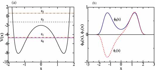
where xπ‘₯x (y𝑦y) stands for coordinate of a particle of mass M𝑀M (mπ‘šm) in DW (HO) potential; pxsubscript𝑝π‘₯p_{x} (pysubscript𝑝𝑦p_{y}) means relevant momentum; V​(x)𝑉π‘₯V(x) signifies the Razavy DW potential Razavy80 ; Ο‰πœ”\omega expresses the oscillator frequency of HO; and DW and HO are coupled by linear (d=1𝑑1d=1) and quadratic (d=2𝑑2d=2) couplings with an interaction strength of c𝑐c. The Razavy potential V​(x)𝑉π‘₯V(x) with adopted parameters of M=ΞΎ=ℏ=1.0π‘€πœ‰Planck-constant-over-2-pi1.0M=\xi=\hbar=1.0 is plotted in Fig. 1(a). Minima of V​(x)𝑉π‘₯V(x) locate at xs=Β±1.38433subscriptπ‘₯𝑠plus-or-minus1.38433x_{s}=\pm 1.38433 with V​(xs)=βˆ’8.125𝑉subscriptπ‘₯𝑠8.125V(x_{s})=-8.125 and its maximum is V​(0)=βˆ’2.0𝑉02.0V(0)=-2.0 at x=0π‘₯0x=0.

First we consider the case of c=0.0𝑐0.0c=0.0 in Eq. (1). Eigenvalues of a DW system with the Razavy DW potential [Eq. (2)] are given by Razavy80

Ο΅0subscriptitalic-Ο΅0\displaystyle\epsilon_{0} =\displaystyle= ℏ22​M​[βˆ’ΞΎβˆ’5βˆ’2​4βˆ’2​ξ+ΞΎ2],superscriptPlanck-constant-over-2-pi22𝑀delimited-[]πœ‰5242πœ‰superscriptπœ‰2\displaystyle\frac{\hbar^{2}}{2M}\left[-\xi-5-2\sqrt{4-2\xi+\xi^{2}}\right], (3)
Ο΅1subscriptitalic-Ο΅1\displaystyle\epsilon_{1} =\displaystyle= ℏ22​M​[ΞΎβˆ’5βˆ’2​4+2​ξ+ΞΎ2],superscriptPlanck-constant-over-2-pi22𝑀delimited-[]πœ‰5242πœ‰superscriptπœ‰2\displaystyle\frac{\hbar^{2}}{2M}\left[\xi-5-2\sqrt{4+2\xi+\xi^{2}}\right], (4)
Ο΅2subscriptitalic-Ο΅2\displaystyle\epsilon_{2} =\displaystyle= ℏ22​M​[βˆ’ΞΎβˆ’5+2​4βˆ’2​ξ+ΞΎ2],superscriptPlanck-constant-over-2-pi22𝑀delimited-[]πœ‰5242πœ‰superscriptπœ‰2\displaystyle\frac{\hbar^{2}}{2M}\left[-\xi-5+2\sqrt{4-2\xi+\xi^{2}}\right], (5)
Ο΅3subscriptitalic-Ο΅3\displaystyle\epsilon_{3} =\displaystyle= ℏ22​M​[ΞΎβˆ’5+2​4+2​ξ+ΞΎ2].superscriptPlanck-constant-over-2-pi22𝑀delimited-[]πœ‰5242πœ‰superscriptπœ‰2\displaystyle\frac{\hbar^{2}}{2M}\left[\xi-5+2\sqrt{4+2\xi+\xi^{2}}\right]. (6)

Eigenvalues for the adopted parameters are Ο΅0=βˆ’4.73205subscriptitalic-Ο΅04.73205\epsilon_{0}=-4.73205, Ο΅1=βˆ’4.64575subscriptitalic-Ο΅14.64575\epsilon_{1}=-4.64575, Ο΅2=βˆ’1.26795subscriptitalic-Ο΅21.26795\epsilon_{2}=-1.26795 and Ο΅3=0.645751subscriptitalic-Ο΅30.645751\epsilon_{3}=0.645751, which lead to

Ο΅italic-Ο΅\displaystyle\epsilon =\displaystyle= Ο΅1+Ο΅0=βˆ’9.3778,subscriptitalic-Ο΅1subscriptitalic-Ο΅09.3778\displaystyle\epsilon_{1}+\epsilon_{0}=-9.3778, (7)
δ𝛿\displaystyle\delta =\displaystyle= Ο΅1βˆ’Ο΅0=0.0863.subscriptitalic-Ο΅1subscriptitalic-Ο΅00.0863\displaystyle\epsilon_{1}-\epsilon_{0}=0.0863. (8)

Figure 1(a) shows that both Ο΅0subscriptitalic-Ο΅0\epsilon_{0} and Ο΅1subscriptitalic-Ο΅1\epsilon_{1} locate below V​(0)𝑉0V(0) and that Ο΅2subscriptitalic-Ο΅2\epsilon_{2} and Ο΅3subscriptitalic-Ο΅3\epsilon_{3} are far above Ο΅1subscriptitalic-Ο΅1\epsilon_{1}. In this study, we take into account the lowest two states of Ο΅0subscriptitalic-Ο΅0\epsilon_{0} and Ο΅1subscriptitalic-Ο΅1\epsilon_{1} whose eigenfunctions are given by Razavy80

Ο•0​(x)subscriptitalic-Ο•0π‘₯\displaystyle\phi_{0}(x) =\displaystyle= A0​eβˆ’ΞΎβ€‹cosh​ 2​x/4​[3​ξ​cosh​x+(4βˆ’ΞΎ+2​4βˆ’2​ξ+ΞΎ2)​cosh​ 3​x],subscript𝐴0superscriptπ‘’πœ‰cosh2π‘₯4delimited-[]3πœ‰coshπ‘₯4πœ‰242πœ‰superscriptπœ‰2cosh3π‘₯\displaystyle A_{0}\;e^{-\xi\>{\rm cosh}\>2x/4}\left[3\xi\>{\rm cosh}\>x+(4-\xi+2\sqrt{4-2\xi+\xi^{2}})\>{\rm cosh}\>3x\right], (9)
Ο•1​(x)subscriptitalic-Ο•1π‘₯\displaystyle\phi_{1}(x) =\displaystyle= A1​eβˆ’ΞΎβ€‹cosh​ 2​x/4​[3​ξ​sinh​x+(4+ΞΎ+2​4+2​ξ+ΞΎ2)​sinh​ 3​x],subscript𝐴1superscriptπ‘’πœ‰cosh2π‘₯4delimited-[]3πœ‰sinhπ‘₯4πœ‰242πœ‰superscriptπœ‰2sinh3π‘₯\displaystyle A_{1}\;e^{-\xi\>{\rm cosh}\>2x/4}\left[3\xi\>{\rm sinh}\>x+(4+\xi+2\sqrt{4+2\xi+\xi^{2}})\>{\rm sinh}\>3x\right], (10)

AΞ½subscript𝐴𝜈A_{\nu} (Ξ½=0,1𝜈01\nu=0,1) denoting normalization factors. Figure 1(b) shows the eigenfunctions of Ο•0​(x)subscriptitalic-Ο•0π‘₯\phi_{0}(x) and Ο•1​(x)subscriptitalic-Ο•1π‘₯\phi_{1}(x), which are symmetric and anti-symmetric, respectively, with respect to the origin.
Refer to caption
Figure 1: (Color online) (a) The Razavy DW potential V​(x)𝑉π‘₯V(x) [Eq.(2)] with eigenvalues of ϡνsubscriptitalic-ϡ𝜈\epsilon_{\nu} (Ξ½=0βˆ’3𝜈03\nu=0-3) for ℏ=M=ΞΎ=1.0Planck-constant-over-2-piπ‘€πœ‰1.0\hbar=M=\xi=1.0. (b) Eigenfunctions of Ο•0​(x)subscriptitalic-Ο•0π‘₯\phi_{0}(x) (solid curve) and Ο•1​(x)subscriptitalic-Ο•1π‘₯\phi_{1}(x) (dashed curve).

The DW system in Eq. (1) is coupled to a harmonic oscillator whose eigenfunction and eigenvalue are given by

ψn​(y)subscriptπœ“π‘›π‘¦\displaystyle\psi_{n}(y) =\displaystyle= 12n​n!​(m​ωπ​ℏ)1/4​exp⁑(βˆ’m​ω​y22​ℏ)​Hn​(m​ωℏ​y),1superscript2𝑛𝑛superscriptπ‘šπœ”πœ‹Planck-constant-over-2-pi14π‘šπœ”superscript𝑦22Planck-constant-over-2-pisubscriptπ»π‘›π‘šπœ”Planck-constant-over-2-pi𝑦\displaystyle\frac{1}{\sqrt{2^{n}n!}}\left(\frac{m\omega}{\pi\hbar}\right)^{1/4}\exp\left(-\frac{m\omega y^{2}}{2\hbar}\right)H_{n}\left(\sqrt{\frac{m\omega}{\hbar}}\>y\right), (11)
ensubscript𝑒𝑛\displaystyle e_{n} =\displaystyle= (n+12)​ℏ​ω(n=0,1,2β‹…,β‹―),𝑛12Planck-constant-over-2-piπœ”(n=0,1,2β‹…,β‹―)\displaystyle\left(n+\frac{1}{2}\right)\hbar\omega\hskip 28.45274pt\mbox{($n=0,1,2\cdot,\cdot\cdot\cdot$)}, (12)

Hn​(y)subscript𝐻𝑛𝑦H_{n}(y) standing for the Hermite polynomial.

II.2 Stationary properties

We calculate eigenvalues and eigenstates of the coupled DW system described by Eq. (1). We expand the wavefunction with basis states of |ν​n⟩=ϕν​(x)β€‹Οˆn​(y)ketπœˆπ‘›subscriptitalic-Ο•πœˆπ‘₯subscriptπœ“π‘›π‘¦|\nu\>n\rangle=\phi_{\nu}(x)\psi_{n}(y) (Ξ½=0,1𝜈01\nu=0,1 and n=0𝑛0n=0 to N𝑁N) as

Φ​(x,y)Ξ¦π‘₯𝑦\displaystyle\Phi(x,y) =\displaystyle= βˆ‘Ξ½=01βˆ‘n=0NcΞ½,n​ϕν​(x)β€‹Οˆn​(y),superscriptsubscript𝜈01superscriptsubscript𝑛0𝑁subscriptπ‘πœˆπ‘›subscriptitalic-Ο•πœˆπ‘₯subscriptπœ“π‘›π‘¦\displaystyle\sum_{\nu=0}^{1}\sum_{n=0}^{N}\>c_{\nu,n}\>\phi_{\nu}(x)\psi_{n}(y), (13)

where N𝑁N denotes the maximum quantum number of HO. We obtain the secular equation

E​cΞ½,n=βˆ‘ΞΌ=01βˆ‘k=0NβŸ¨Ξ½β€‹n|H|μ​kβŸ©β€‹cΞΌ,k,𝐸subscriptπ‘πœˆπ‘›superscriptsubscriptπœ‡01superscriptsubscriptπ‘˜0𝑁quantum-operator-productπœˆπ‘›π»πœ‡π‘˜subscriptπ‘πœ‡π‘˜\displaystyle E\>c_{\nu,n}=\sum_{\mu=0}^{1}\sum_{k=0}^{N}\>\langle\nu\>n|H|\mu\>k\rangle\;c_{\mu,k}, (14)

where

βŸ¨Ξ½β€‹n|H|μ​k⟩quantum-operator-productπœˆπ‘›π»πœ‡π‘˜\displaystyle\langle\nu\>n|H|\mu\>k\rangle =\displaystyle= [ϡν+(n+12)​ℏ​ω]​δν,μ​δn,kdelimited-[]subscriptitalic-Ο΅πœˆπ‘›12Planck-constant-over-2-piπœ”subscriptπ›Ώπœˆπœ‡subscriptπ›Ώπ‘›π‘˜\displaystyle\left[\epsilon_{\nu}+\left(n+\frac{1}{2}\right)\hbar\omega\right]\>\delta_{\nu,\mu}\>\delta_{n,k} (15)
βˆ’\displaystyle- [Ξ΄d,1​΢​(δν,ΞΌ+1+δν,ΞΌβˆ’1)+Ξ΄d,2​δν,μ​(ΞΆ0​δν,0+ΞΆ1​δν,1)]delimited-[]subscript𝛿𝑑1𝜁subscriptπ›Ώπœˆπœ‡1subscriptπ›Ώπœˆπœ‡1subscript𝛿𝑑2subscriptπ›Ώπœˆπœ‡subscript𝜁0subscriptπ›Ώπœˆ0subscript𝜁1subscriptπ›Ώπœˆ1\displaystyle\left[\delta_{d,1}\;\zeta\left(\delta_{\nu,\mu+1}+\delta_{\nu,\mu-1}\right)+\delta_{d,2}\;\delta_{\nu,\mu}\>\left(\zeta_{0}\>\delta_{\nu,0}+\zeta_{1}\>\delta_{\nu,1}\right)\right]
Γ—\displaystyle\times (n​δn,k+1+n+1​δn,kβˆ’1),𝑛subscriptπ›Ώπ‘›π‘˜1𝑛1subscriptπ›Ώπ‘›π‘˜1\displaystyle\left(\sqrt{n}\>\delta_{n,k+1}+\sqrt{n+1}\>\delta_{n,k-1}\right),

with

΢𝜁\displaystyle\zeta =\displaystyle= c​γ​g2,𝑐𝛾𝑔2\displaystyle c\>\gamma\>\sqrt{\frac{g}{2}}, (16)
ΞΆΞ»subscriptπœπœ†\displaystyle\zeta_{\lambda} =\displaystyle= c​γλ​g2,(Ξ»=0,1;g=ℏ/m​ω)𝑐subscriptπ›Ύπœ†π‘”2formulae-sequenceπœ†01𝑔Planck-constant-over-2-piπ‘šπœ”\displaystyle c\>\gamma_{\lambda}\>\sqrt{\frac{g}{2}},\hskip 28.45274pt\left(\lambda=0,1;\;\;g=\sqrt{\hbar/m\omega}\right) (17)
γ𝛾\displaystyle\gamma =\displaystyle= βˆ«βˆ’βˆžβˆžΟ•0​(x)​x​ϕ1​(x)​𝑑x=1.13823,superscriptsubscriptsubscriptitalic-Ο•0π‘₯π‘₯subscriptitalic-Ο•1π‘₯differential-dπ‘₯1.13823\displaystyle\int_{-\infty}^{\infty}\>\phi_{0}(x)\>x\>\phi_{1}(x)\>dx=1.13823, (18)
Ξ³0subscript𝛾0\displaystyle\gamma_{0} =\displaystyle= βˆ«βˆ’βˆžβˆžΟ•0​(x)​x2​ϕ0​(x)​𝑑x=1.36128,superscriptsubscriptsubscriptitalic-Ο•0π‘₯superscriptπ‘₯2subscriptitalic-Ο•0π‘₯differential-dπ‘₯1.36128\displaystyle\int_{-\infty}^{\infty}\>\phi_{0}(x)\>x^{2}\>\phi_{0}(x)\>dx=1.36128, (19)
Ξ³1subscript𝛾1\displaystyle\gamma_{1} =\displaystyle= βˆ«βˆ’βˆžβˆžΟ•1​(x)​x2​ϕ1​(x)​𝑑x=1.44467.superscriptsubscriptsubscriptitalic-Ο•1π‘₯superscriptπ‘₯2subscriptitalic-Ο•1π‘₯differential-dπ‘₯1.44467\displaystyle\int_{-\infty}^{\infty}\>\phi_{1}(x)\>x^{2}\>\phi_{1}(x)\>dx=1.44467. (20)

From a diagonalization of the secular equation (14), we may obtain the eigenvalue EΞΊsubscriptπΈπœ…E_{\kappa} and eigenfunction Ψκ​(x,y)subscriptΞ¨πœ…π‘₯𝑦\Psi_{\kappa}(x,y) satisfying the stationary SchrΓΆdinger equation

H​Φκ​(x,y)=Eκ​Φκ​(x,y),𝐻subscriptΞ¦πœ…π‘₯𝑦subscriptπΈπœ…subscriptΞ¦πœ…π‘₯𝑦\displaystyle H\Phi_{\kappa}(x,y)=E_{\kappa}\Phi_{\kappa}(x,y), (21)

where ΞΊ=0πœ…0\kappa=0 to Nmsubscriptπ‘π‘šN_{m} =2​(N+1)βˆ’1absent2𝑁11=2(N+1)-1. Eigenvalues and eigenfunctions for N=1𝑁1N=1 are analytically obtained, and those for N>1𝑁1N>1 are evaluated by MATHEMATICA.

II.3 Dynamical properties

In the spectral method, a solution of the time-dependent SchrΓΆdinger equation

iβ€‹β„β€‹βˆ‚Ξ¨β€‹(x,y,t)βˆ‚t𝑖Planck-constant-over-2-piΞ¨π‘₯𝑦𝑑𝑑\displaystyle i\hbar\frac{\partial\Psi(x,y,t)}{\partial t} =\displaystyle= H​Ψ​(x,y,t),𝐻Ψπ‘₯𝑦𝑑\displaystyle H\Psi(x,y,t), (22)

is expressed by

Ψ​(x,y,t)Ξ¨π‘₯𝑦𝑑\displaystyle\Psi(x,y,t) =\displaystyle= βˆ‘ΞΊ=0Nmaκ​Φκ​(x,y)​eβˆ’i​Eκ​t/ℏ,superscriptsubscriptπœ…0subscriptπ‘π‘šsubscriptπ‘Žπœ…subscriptΞ¦πœ…π‘₯𝑦superscript𝑒𝑖subscriptπΈπœ…π‘‘Planck-constant-over-2-pi\displaystyle\sum_{\kappa=0}^{N_{m}}\>a_{\kappa}\>\Phi_{\kappa}(x,y)\>e^{-iE_{\kappa}t/\hbar}, (23)

with

βˆ‘ΞΊ=0Nm|aΞΊ|2superscriptsubscriptπœ…0subscriptπ‘π‘šsuperscriptsubscriptπ‘Žπœ…2\displaystyle\sum_{\kappa=0}^{N_{m}}|a_{\kappa}|^{2} =\displaystyle= 1,1\displaystyle 1, (24)

where EΞΊsubscriptπΈπœ…E_{\kappa} and Φκ​(x,y)subscriptΞ¦πœ…π‘₯𝑦\Phi_{\kappa}(x,y) are eigenvalue and eigenfunction, respectively, obtained in Eq. (21). Expansion coefficients aΞΊsubscriptπ‘Žπœ…a_{\kappa} are in principle determined by a given initial wavepacket, which requires cumbersome calculations. Instead we adopt in this study, a conventional wavepacket with coefficients given by a0=a1=1/2subscriptπ‘Ž0subscriptπ‘Ž112a_{0}=a_{1}=1/\sqrt{2} and aΞΊ=0subscriptπ‘Žπœ…0a_{\kappa}=0 for ΞΊβ‰₯2πœ…2\kappa\geq 2,

Ψ​(x,y,t)Ξ¨π‘₯𝑦𝑑\displaystyle\Psi(x,y,t) =\displaystyle= 12​[Ξ¦0​(x,y)​eβˆ’i​E0​t/ℏ+Ξ¦1​(x,y)​eβˆ’i​E1​t/ℏ].12delimited-[]subscriptΞ¦0π‘₯𝑦superscript𝑒𝑖subscript𝐸0𝑑Planck-constant-over-2-pisubscriptΞ¦1π‘₯𝑦superscript𝑒𝑖subscript𝐸1𝑑Planck-constant-over-2-pi\displaystyle\frac{1}{\sqrt{2}}\left[\Phi_{0}(x,y)\>e^{-iE_{0}t/\hbar}+\Phi_{1}(x,y)\>e^{-iE_{1}t/\hbar}\right]. (25)

The tunneling period T𝑇T for the wavepacket given by Eq. (25) is determined by

T𝑇\displaystyle T =\displaystyle= 2​π​ℏE1βˆ’E0=2​πΩ1,2πœ‹Planck-constant-over-2-pisubscript𝐸1subscript𝐸02πœ‹subscriptΞ©1\displaystyle\frac{2\pi\hbar}{E_{1}-E_{0}}=\frac{2\pi}{\Omega_{1}}, (26)

where Ξ©1=(E1βˆ’E0)/ℏsubscriptΞ©1subscript𝐸1subscript𝐸0Planck-constant-over-2-pi\Omega_{1}=(E_{1}-E_{0})/\hbar. We will study a wavepacket with a0=a1=a2=a3=1/2subscriptπ‘Ž0subscriptπ‘Ž1subscriptπ‘Ž2subscriptπ‘Ž312a_{0}=a_{1}=a_{2}=a_{3}=1/2 in Sec. IV A, whose tunneling period is not given by Eq. (26).

III Model calculations

Introducing a parameter α𝛼\alpha, we express the harmonic oscillator frequency Ο‰πœ”\omega by

ℏ​ωPlanck-constant-over-2-piπœ”\displaystyle\hbar\omega =\displaystyle= α​(Ο΅1βˆ’Ο΅0)=α​δ.𝛼subscriptitalic-Ο΅1subscriptitalic-Ο΅0𝛼𝛿\displaystyle\alpha(\epsilon_{1}-\epsilon_{0})=\alpha\>\delta. (27)

Coefficients of ΢𝜁\zeta, ΞΆ0subscript𝜁0\zeta_{0} and ΞΆ1subscript𝜁1\zeta_{1} in Eqs. (16) and (17) are expressed in terms of mπ‘šm, α𝛼\alpha and c𝑐c as follows:

΢𝜁\displaystyle\zeta =\displaystyle= c​γ​(ℏ24​m​α​δ)1/4=c​(γ​ℏ2​δ1/4)​(1m​α)1/4=1.485​c​(1m​α)1/4,𝑐𝛾superscriptsuperscriptPlanck-constant-over-2-pi24π‘šπ›Όπ›Ώ14𝑐𝛾Planck-constant-over-2-pi2superscript𝛿14superscript1π‘šπ›Ό141.485𝑐superscript1π‘šπ›Ό14\displaystyle c\>\gamma\left(\frac{\hbar^{2}}{4m\alpha\delta}\right)^{1/4}=c\left(\frac{\gamma\sqrt{\hbar}}{\sqrt{2}\>\delta^{1/4}}\right)\>\left(\frac{1}{m\alpha}\right)^{1/4}=1.485\>c\>\left(\frac{1}{m\alpha}\right)^{1/4}, (28)
ΞΆ0subscript𝜁0\displaystyle\zeta_{0} =\displaystyle= c​(Ξ³0​ℏ2​δ1/4)​(1m​α)1/4=1.776​c​(1m​α)1/4,𝑐subscript𝛾0Planck-constant-over-2-pi2superscript𝛿14superscript1π‘šπ›Ό141.776𝑐superscript1π‘šπ›Ό14\displaystyle c\left(\frac{\gamma_{0}\sqrt{\hbar}}{\sqrt{2}\>\delta^{1/4}}\right)\>\left(\frac{1}{m\alpha}\right)^{1/4}=1.776\>c\>\left(\frac{1}{m\alpha}\right)^{1/4}, (29)
ΞΆ1subscript𝜁1\displaystyle\zeta_{1} =\displaystyle= c​(Ξ³1​ℏ2​δ1/4)​(1m​α)1/4=1.885​c​(1m​α)1/4.𝑐subscript𝛾1Planck-constant-over-2-pi2superscript𝛿14superscript1π‘šπ›Ό141.885𝑐superscript1π‘šπ›Ό14\displaystyle c\left(\frac{\gamma_{1}\sqrt{\hbar}}{\sqrt{2}\>\delta^{1/4}}\right)\>\left(\frac{1}{m\alpha}\right)^{1/4}=1.885\>c\>\left(\frac{1}{m\alpha}\right)^{1/4}. (30)

Table 1 summarizes various coefficients appearing in our model calculations. δ𝛿\delta, γ𝛾\gamma, Ξ³0subscript𝛾0\gamma_{0}, Ξ³1subscript𝛾1\gamma_{1} and Ξ·πœ‚\eta are determined by the Razavy potential with M=ΞΎ=1.0π‘€πœ‰1.0M=\xi=1.0 whereas Ξ³ysubscript𝛾𝑦\gamma_{y} and Ξ·ysubscriptπœ‚π‘¦\eta_{y} are given by HO potential with m=1.0π‘š1.0m=1.0 and Ο‰=Ξ±β€‹Ξ΄πœ”π›Όπ›Ώ\omega=\alpha\delta (Ξ±=10.0𝛼10.0\alpha=10.0). Then model calculations to be reported will be specified by a set of parameters of mπ‘šm, α𝛼\alpha, c𝑐c and N𝑁N.

Coefficient Definition Value Note
δ𝛿\;\;\;\delta\;\;\; Ο΅1βˆ’Ο΅0subscriptitalic-Ο΅1subscriptitalic-Ο΅0\epsilon_{1}-\epsilon_{0}   0.086300.08630\;\;0.08630\;\; β€…β€…β€…Eq. (8)
γ𝛾\;\;\;\gamma\;\;\; βŸ¨Ο•0​x​ϕ1⟩xsubscriptdelimited-⟨⟩subscriptitalic-Ο•0π‘₯subscriptitalic-Ο•1π‘₯\langle\phi_{0}\>x\>\phi_{1}\rangle_{x}   1.13821.1382\;\;1.1382\;\; Eq. (18)
Ξ³0subscript𝛾0\gamma_{0} βŸ¨Ο•0​x2​ϕ0⟩xsubscriptdelimited-⟨⟩subscriptitalic-Ο•0superscriptπ‘₯2subscriptitalic-Ο•0π‘₯\;\;\langle\phi_{0}\>x^{2}\>\phi_{0}\rangle_{x}\;\; 1.36131.36131.3613 Eq. (19)
Ξ³1subscript𝛾1\gamma_{1} βŸ¨Ο•1​x2​ϕ1⟩xsubscriptdelimited-⟨⟩subscriptitalic-Ο•1superscriptπ‘₯2subscriptitalic-Ο•1π‘₯\langle\phi_{1}\>x^{2}\>\phi_{1}\rangle_{x} 1.44471.44471.4447 Eq. (20)
Ξ·πœ‚\eta βŸ¨Ο•0β€‹βˆ‚xΟ•1⟩xsubscriptdelimited-⟨⟩subscriptitalic-Ο•0subscriptπ‘₯subscriptitalic-Ο•1π‘₯\langle\phi_{0}\>\partial_{x}\phi_{1}\rangle_{x} 0.098230.098230.09823 Eq. (60)
Ξ³ysubscript𝛾𝑦\gamma_{y} ⟨ψ0​yβ€‹Οˆ1⟩ysubscriptdelimited-⟨⟩subscriptπœ“0𝑦subscriptπœ“1𝑦\langle\psi_{0}\>y\>\psi_{1}\rangle_{y} 0.761170.761170.76117 Eq. (61)
Ξ·ysubscriptπœ‚π‘¦\eta_{y} ⟨ψ0β€‹βˆ‚yψ1⟩ysubscriptdelimited-⟨⟩subscriptπœ“0subscript𝑦subscriptπœ“1𝑦\langle\psi_{0}\>\partial_{y}\psi_{1}\rangle_{y} 0.656890.656890.65689 Eq. (62)

Table 1 Various coefficients in model calculations with M=ΞΎ=m=ℏ=1.0π‘€πœ‰π‘šPlanck-constant-over-2-pi1.0M=\xi=m=\hbar=1.0 and Ξ±=10.0𝛼10.0\alpha=10.0, βŸ¨β‹…βŸ©xsubscriptdelimited-βŸ¨βŸ©β‹…π‘₯\langle\cdot\rangle_{x} and βŸ¨β‹…βŸ©ysubscriptdelimited-βŸ¨βŸ©β‹…π‘¦\langle\cdot\rangle_{y} denoting integrals over xπ‘₯x and y𝑦y, respectively (see text).

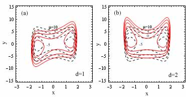
Figures 2(a) and 2(a) show contour maps of the composite potential U​(x,y)=ΞΌπ‘ˆπ‘₯π‘¦πœ‡U(x,y)=\mu defined by

U​(x,y)π‘ˆπ‘₯𝑦\displaystyle U(x,y) =\displaystyle= V​(x)+m​ω2​y22βˆ’c​xd​y,𝑉π‘₯π‘šsuperscriptπœ”2superscript𝑦22𝑐superscriptπ‘₯𝑑𝑦\displaystyle V(x)+\frac{m\omega^{2}y^{2}}{2}-c\>x^{d}\;y, (31)

for linear (d=1𝑑1d=1) and quadratic (d=2𝑑2d=2) couplings, respectively, with c=0.0𝑐0.0c=0.0 (dashed curves) and c=1.0𝑐1.0c=1.0 (solid curves) for ΞΌ=βˆ’5.0πœ‡5.0\mu=-5.0, 0.0, 5.0 and 10.0 (m=1.0π‘š1.0m=1.0 and Ξ±=10.0𝛼10.0\alpha=10.0). For c=0𝑐0c=0, U​(x,y)π‘ˆπ‘₯𝑦U(x,y) has two minima of U​(x,y)=βˆ’8.125π‘ˆπ‘₯𝑦8.125U(x,y)=-8.125 at (x,y)=(Β±1.3843, 0.0)π‘₯𝑦plus-or-minus1.38430.0(x,y)=(\pm 1.3843,\;0.0). For a linear coupling (d=1𝑑1d=1) with c=1.0𝑐1.0c=1.0, it has two minima of U​(x,y)=βˆ’9.438π‘ˆπ‘₯𝑦9.438U(x,y)=-9.438 at (x,y)=(1.4120, 1.8959)π‘₯𝑦1.41201.8959(x,y)=(1.4120,\;1.8959) and (βˆ’1.4120,βˆ’1.8959)1.41201.8959(-1.4120,\;-1.8959). For a quadratic coupling (d=2𝑑2d=2) with c=1.0𝑐1.0c=1.0, it has two minima of U​(x,y)=βˆ’9.125π‘ˆπ‘₯𝑦9.125U(x,y)=-9.125 at (x,y)=(1.4120, 1.8959)π‘₯𝑦1.41201.8959(x,y)=(1.4120,\;1.8959) and (βˆ’1.4120, 1.8959)1.41201.8959(-1.4120,\;1.8959). Model calculations for linear and quadratic couplings with N=1𝑁1N=1 will be separately reported in Secs. III A and III B, respectively.
Refer to caption
Figure 2: (Color online) Contour plots of U​(x,y)=ΞΌπ‘ˆπ‘₯π‘¦πœ‡U(x,y)=\mu with ΞΌ=βˆ’5πœ‡5\mu=-5, 00, 555 and 101010 (from the inside) for (a) linear (d=1𝑑1d=1) and (b) quadratic (d=2𝑑2d=2) couplings with c=0.0𝑐0.0c=0.0 (dashed curves) and c=1.0𝑐1.0c=1.0 (solid curves).

III.1 Linear coupling with N=1𝑁1N=1

For a linear coupling (d=1𝑑1d=1) with N=1𝑁1N=1, the energy matrix of the Hamiltonian given by Eq. (1) is expressed in the basis of ψ0​(y)​ϕ0​(x)subscriptπœ“0𝑦subscriptitalic-Ο•0π‘₯\psi_{0}(y)\phi_{0}(x), ψ0​(y)​ϕ1​(x)subscriptπœ“0𝑦subscriptitalic-Ο•1π‘₯\psi_{0}(y)\phi_{1}(x), ψ1​(y)​ϕ0​(x)subscriptπœ“1𝑦subscriptitalic-Ο•0π‘₯\psi_{1}(y)\phi_{0}(x) and ψ1​(y)​ϕ1​(x)subscriptπœ“1𝑦subscriptitalic-Ο•1π‘₯\psi_{1}(y)\phi_{1}(x) by

β„‹β„‹\displaystyle{\cal H} =\displaystyle= (Ο΅0+ℏ​ω/200βˆ’ΞΆ0Ο΅1+ℏ​ω/2βˆ’ΞΆ00βˆ’ΞΆΟ΅0+3​ℏ​ω/20βˆ’ΞΆ00Ο΅1+3​ℏ​ω/2),subscriptitalic-Ο΅0Planck-constant-over-2-piπœ”200𝜁missing-subexpressionmissing-subexpressionmissing-subexpressionmissing-subexpressionmissing-subexpressionmissing-subexpressionmissing-subexpressionmissing-subexpressionmissing-subexpressionmissing-subexpressionmissing-subexpressionmissing-subexpressionmissing-subexpressionmissing-subexpressionmissing-subexpressionmissing-subexpression0subscriptitalic-Ο΅1Planck-constant-over-2-piπœ”2𝜁0missing-subexpressionmissing-subexpressionmissing-subexpressionmissing-subexpressionmissing-subexpressionmissing-subexpressionmissing-subexpressionmissing-subexpressionmissing-subexpressionmissing-subexpressionmissing-subexpressionmissing-subexpressionmissing-subexpressionmissing-subexpressionmissing-subexpressionmissing-subexpression0𝜁subscriptitalic-Ο΅03Planck-constant-over-2-piπœ”20missing-subexpressionmissing-subexpressionmissing-subexpressionmissing-subexpressionmissing-subexpressionmissing-subexpressionmissing-subexpressionmissing-subexpressionmissing-subexpressionmissing-subexpressionmissing-subexpressionmissing-subexpressionmissing-subexpressionmissing-subexpressionmissing-subexpressionmissing-subexpression𝜁00subscriptitalic-Ο΅13Planck-constant-over-2-piπœ”2missing-subexpressionmissing-subexpressionmissing-subexpressionmissing-subexpressionmissing-subexpressionmissing-subexpressionmissing-subexpressionmissing-subexpressionmissing-subexpressionmissing-subexpressionmissing-subexpressionmissing-subexpressionmissing-subexpressionmissing-subexpressionmissing-subexpressionmissing-subexpression\displaystyle\left({\begin{array}[]{*{20}c}{\epsilon_{0}+\hbar\omega/2}&{0}&{0}&{-\zeta}\\ {0}&{\epsilon_{1}+\hbar\omega/2}&{-\zeta}&{0}\\ {0}&{-\zeta}&{\epsilon_{0}+3\hbar\omega/2}&{0}\\ {-\zeta}&{0}&{0}&{\epsilon_{1}+3\hbar\omega/2}\\ \end{array}}\right), (36)

where ΢𝜁\zeta is given by Eq. (28). We obtain eigenvalues of the energy matrix

E0subscript𝐸0\displaystyle E_{0} =\displaystyle= Ο΅2+β„β€‹Ο‰βˆ’14​(ℏ​ω+Ξ΄)2+ΞΆ2,italic-Ο΅2Planck-constant-over-2-piπœ”14superscriptPlanck-constant-over-2-piπœ”π›Ώ2superscript𝜁2\displaystyle\frac{\epsilon}{2}+\hbar\omega-\sqrt{\frac{1}{4}(\hbar\omega+\delta)^{2}+\zeta^{2}}, (37)
E1subscript𝐸1\displaystyle E_{1} =\displaystyle= Ο΅2+β„β€‹Ο‰βˆ’14​(β„β€‹Ο‰βˆ’Ξ΄)2+ΞΆ2,italic-Ο΅2Planck-constant-over-2-piπœ”14superscriptPlanck-constant-over-2-piπœ”π›Ώ2superscript𝜁2\displaystyle\frac{\epsilon}{2}+\hbar\omega-\sqrt{\frac{1}{4}(\hbar\omega-\delta)^{2}+\zeta^{2}}, (38)
E2subscript𝐸2\displaystyle E_{2} =\displaystyle= Ο΅2+ℏ​ω+14​(β„β€‹Ο‰βˆ’Ξ΄)2+ΞΆ2,italic-Ο΅2Planck-constant-over-2-piπœ”14superscriptPlanck-constant-over-2-piπœ”π›Ώ2superscript𝜁2\displaystyle\frac{\epsilon}{2}+\hbar\omega+\sqrt{\frac{1}{4}(\hbar\omega-\delta)^{2}+\zeta^{2}}, (39)
E3subscript𝐸3\displaystyle E_{3} =\displaystyle= Ο΅2+ℏ​ω+14​(ℏ​ω+Ξ΄)2+ΞΆ2.italic-Ο΅2Planck-constant-over-2-piπœ”14superscriptPlanck-constant-over-2-piπœ”π›Ώ2superscript𝜁2\displaystyle\frac{\epsilon}{2}+\hbar\omega+\sqrt{\frac{1}{4}(\hbar\omega+\delta)^{2}+\zeta^{2}}. (40)

Relevant eigenfunctions are expressed by

Ξ¦0​(x,y)subscriptΞ¦0π‘₯𝑦\displaystyle\Phi_{0}(x,y) =\displaystyle= cos⁑θ1β€‹Οˆ0​(y)​ϕ0​(x)+sin⁑θ1β€‹Οˆ1​(y)​ϕ1​(x),subscriptπœƒ1subscriptπœ“0𝑦subscriptitalic-Ο•0π‘₯subscriptπœƒ1subscriptπœ“1𝑦subscriptitalic-Ο•1π‘₯\displaystyle\cos\theta_{1}\>\psi_{0}(y)\phi_{0}(x)+\sin\theta_{1}\>\psi_{1}(y)\phi_{1}(x), (41)
Ξ¦1​(x,y)subscriptΞ¦1π‘₯𝑦\displaystyle\Phi_{1}(x,y) =\displaystyle= cos⁑θ2β€‹Οˆ0​(y)​ϕ1​(x)+sin⁑θ2β€‹Οˆ1​(y)​ϕ0​(x),subscriptπœƒ2subscriptπœ“0𝑦subscriptitalic-Ο•1π‘₯subscriptπœƒ2subscriptπœ“1𝑦subscriptitalic-Ο•0π‘₯\displaystyle\cos\theta_{2}\>\psi_{0}(y)\phi_{1}(x)+\sin\theta_{2}\>\psi_{1}(y)\phi_{0}(x), (42)
Ξ¦2​(x,y)subscriptΞ¦2π‘₯𝑦\displaystyle\Phi_{2}(x,y) =\displaystyle= βˆ’sin⁑θ2β€‹Οˆ0​(y)​ϕ1​(x)+cos⁑θ2β€‹Οˆ1​(y)​ϕ0​(x),subscriptπœƒ2subscriptπœ“0𝑦subscriptitalic-Ο•1π‘₯subscriptπœƒ2subscriptπœ“1𝑦subscriptitalic-Ο•0π‘₯\displaystyle-\sin\theta_{2}\>\psi_{0}(y)\phi_{1}(x)+\cos\theta_{2}\>\psi_{1}(y)\phi_{0}(x), (43)
Ξ¦3​(x,y)subscriptΞ¦3π‘₯𝑦\displaystyle\Phi_{3}(x,y) =\displaystyle= βˆ’sin⁑θ1β€‹Οˆ0​(y)​ϕ0​(x)+cos⁑θ1β€‹Οˆ1​(y)​ϕ1​(x),subscriptπœƒ1subscriptπœ“0𝑦subscriptitalic-Ο•0π‘₯subscriptπœƒ1subscriptπœ“1𝑦subscriptitalic-Ο•1π‘₯\displaystyle-\sin\theta_{1}\>\psi_{0}(y)\phi_{0}(x)+\cos\theta_{1}\>\psi_{1}(y)\phi_{1}(x), (44)

where

tan⁑ 2​θ12subscriptπœƒ1\displaystyle\tan\>2\theta_{1} =\displaystyle= 2​΢(ℏ​ω+Ξ΄),2𝜁Planck-constant-over-2-piπœ”π›Ώ\displaystyle\frac{2\zeta}{(\hbar\omega+\delta)}, (45)
tan⁑ 2​θ22subscriptπœƒ2\displaystyle\tan\>2\theta_{2} =\displaystyle= 2​΢(β„β€‹Ο‰βˆ’Ξ΄).2𝜁Planck-constant-over-2-piπœ”π›Ώ\displaystyle\frac{2\zeta}{(\hbar\omega-\delta)}. (46)

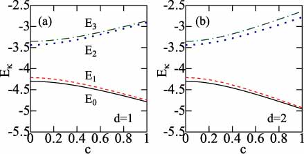
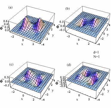
Eigenvalues EΞΊsubscriptπΈπœ…E_{\kappa} (ΞΊ=0βˆ’3πœ…03\kappa=0-3) for d=1𝑑1d=1 with m=1.0π‘š1.0m=1.0 and Ξ±=10.0𝛼10.0\alpha=10.0 are plotted as a function of c𝑐c in Fig. 3(a): Fig. 3(b) for d=2𝑑2d=2 will be explained later (Sec. III B). An energy gap between the ground and first-excited states is Ξ©1=0.08630subscriptΞ©10.08630\Omega_{1}=0.08630 for c=0.0𝑐0.0c=0.0 and Ξ©1=0.03958subscriptΞ©10.03958\Omega_{1}=0.03958 for c=1.0𝑐1.0c=1.0. Ξ©1subscriptΞ©1\Omega_{1} is decreased with increasing c𝑐c. Figures 4(a)-4(d) show 3D plots of eigenfunctions of Φκ​(x,y)subscriptΞ¦πœ…π‘₯𝑦\Phi_{\kappa}(x,y) (ΞΊ=0βˆ’3πœ…03\kappa=0-3).

Refer to caption
Figure 3: (Color online) The c𝑐c dependence of eigenvalues EΞΊsubscriptπΈπœ…E_{\kappa} (ΞΊ=0βˆ’πœ…limit-from0\kappa=0-3) of (a) a linear coupling (d=1𝑑1d=1) and (b) a quadratic coupling (d=2𝑑2d=2) with m=1.0π‘š1.0m=1.0, Ξ±=10.0𝛼10.0\alpha=10.0 and N=1𝑁1N=1.
Refer to caption
Figure 4: (Color online) Eigenfunctions of (a) Ξ¦0​(x,y)subscriptΞ¦0π‘₯𝑦\Phi_{0}(x,y), (b) Ξ¦1​(x,y)subscriptΞ¦1π‘₯𝑦\Phi_{1}(x,y), (c) Ξ¦2​(x,y)subscriptΞ¦2π‘₯𝑦\Phi_{2}(x,y), and (d) Ξ¦3​(x,y)subscriptΞ¦3π‘₯𝑦\Phi_{3}(x,y) for a linear coupling (d=1𝑑1d=1) (m=1.0π‘š1.0m=1.0, Ξ±=10.0𝛼10.0\alpha=10.0, c=1.0𝑐1.0c=1.0 and N=1𝑁1N=1).

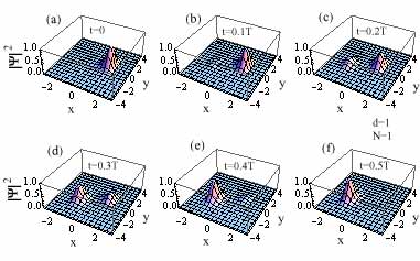
We investigate motion of a wavepacket consisting of Ξ¦0​(x,y)subscriptΞ¦0π‘₯𝑦\Phi_{0}(x,y) and Ξ¦1​(x,y)subscriptΞ¦1π‘₯𝑦\Phi_{1}(x,y) given by Eq. (25). Time-dependent wavepackets are illustrated in Figs. 5(a)-(f) which show 3D plots of |Ψ​(x,y,t)|2superscriptΞ¨π‘₯𝑦𝑑2|\Psi(x,y,t)|^{2} at (a) t=0.0𝑑0.0t=0.0, (b) 0.1​T0.1𝑇0.1T, (c) 0.2​T0.2𝑇0.2T, (d) 0.3​T0.3𝑇0.3T, (e) 0.4​T0.4𝑇0.4T and (f) 0.5​T0.5𝑇0.5T, where T=158.73𝑇158.73T=158.73 obtained by Ξ©1=0.03958subscriptΞ©10.03958\Omega_{1}=0.03958. Wavepackets at t=0.6​T𝑑0.6𝑇t=0.6T, 0.7​T0.7𝑇0.7T, 0.8​T0.8𝑇0.8T, 0.9​T0.9𝑇0.9T and T𝑇T are the same as those at t=0.4​T𝑑0.4𝑇t=0.4T, 0.3​T0.3𝑇0.3T, 0.2​T0.2𝑇0.2T, 0.1​T0.1𝑇0.1T and 0.00.00.0, respectively. At t=0.0𝑑0.0t=0.0, a peak of the wavepacket locates at (xm,ym)=(1.2353,0.61990)subscriptπ‘₯π‘šsubscriptπ‘¦π‘š1.23530.61990(x_{m},y_{m})=(1.2353,0.61990). With time developing, a peak of the wavepacket at (x,y)=(βˆ’1.2353,βˆ’0.61990)π‘₯𝑦1.23530.61990(x,y)=(-1.2353,-0.61990) is growing, and it goes back to the initial position at t=T𝑑𝑇t=T. The wavepacket shows a tunneling from (x,y)=(1.2353,0.61990)π‘₯𝑦1.23530.61990(x,y)=(1.2353,0.61990) to (x,y)=(βˆ’1.2353,βˆ’0.61990)π‘₯𝑦1.23530.61990(x,y)=(-1.2353,-0.61990) across the potential barrier at the origin [see Fig. 2(a)].
Refer to caption
Figure 5: (Color online) |Ψ​(x,y,t)|2superscriptΞ¨π‘₯𝑦𝑑2|\Psi(x,y,t)|^{2} for a linear coupling (d=1𝑑1d=1) at (a) t=0.0𝑑0.0t=0.0, (b) t=0.1​T𝑑0.1𝑇t=0.1T, (c) t=0.2​T𝑑0.2𝑇t=0.2T, (d) t=0.3​T𝑑0.3𝑇t=0.3T, (e) t=0.4​T𝑑0.4𝑇t=0.4T and (f) t=0.5​T𝑑0.5𝑇t=0.5T where T=158.73𝑇158.73T=158.73 (m=1.0π‘š1.0m=1.0, Ξ±=10.0𝛼10.0\alpha=10.0, c=1.0𝑐1.0c=1.0 and N=1𝑁1N=1).
Refer to caption
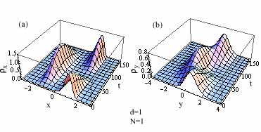
Figure 6: (Color online) Time dependence of (a) ρx​(t)subscript𝜌π‘₯𝑑\rho_{x}(t) and (b) ρy​(t)subscriptπœŒπ‘¦π‘‘\rho_{y}(t) for a linear coupling (d=1𝑑1d=1) (m=1.0π‘š1.0m=1.0, Ξ±=10.0𝛼10.0\alpha=10.0, c=1.0𝑐1.0c=1.0 and N=1𝑁1N=1).
Refer to caption
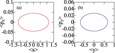
Figure 7: (Color online) Phase space representations of (a) ⟨px⟩delimited-⟨⟩subscript𝑝π‘₯\langle p_{x}\rangle vs. ⟨x⟩delimited-⟨⟩π‘₯\langle x\rangle and (b) ⟨py⟩delimited-⟨⟩subscript𝑝𝑦\langle p_{y}\rangle vs. ⟨y⟩delimited-βŸ¨βŸ©π‘¦\langle y\rangle for a linear coupling (d=1𝑑1d=1) (m=1.0π‘š1.0m=1.0, Ξ±=10.0𝛼10.0\alpha=10.0, c=1.0𝑐1.0c=1.0 and N=1𝑁1N=1).

By using Eqs. (25), (41)-(44), we may calculate marginal probability densities of xπ‘₯x and y𝑦y components, which are given by

ρx​(t)subscript𝜌π‘₯𝑑\displaystyle\rho_{x}(t) =\displaystyle= βˆ«βˆ’βˆžβˆž|Ψ​(x,y,t)|2​𝑑y,superscriptsubscriptsuperscriptΞ¨π‘₯𝑦𝑑2differential-d𝑦\displaystyle\int_{-\infty}^{\infty}\>|\Psi(x,y,t)|^{2}\>dy,
=\displaystyle= 12​(cos2⁑θ1+sin2⁑θ2)​ϕ0​(x)2+12​(sin2⁑θ1+cos2⁑θ2)​ϕ1​(x)212superscript2subscriptπœƒ1superscript2subscriptπœƒ2subscriptitalic-Ο•0superscriptπ‘₯212superscript2subscriptπœƒ1superscript2subscriptπœƒ2subscriptitalic-Ο•1superscriptπ‘₯2\displaystyle\frac{1}{2}\left(\cos^{2}\theta_{1}+\sin^{2}\theta_{2}\right)\phi_{0}(x)^{2}+\frac{1}{2}\left(\sin^{2}\theta_{1}+\cos^{2}\theta_{2}\right)\phi_{1}(x)^{2}
+\displaystyle+ cos⁑(ΞΈ1βˆ’ΞΈ2)​ϕ0​(x)​ϕ1​(x)​cos⁑Ω1​t,subscriptπœƒ1subscriptπœƒ2subscriptitalic-Ο•0π‘₯subscriptitalic-Ο•1π‘₯subscriptΞ©1𝑑\displaystyle\cos(\theta_{1}-\theta_{2})\phi_{0}(x)\phi_{1}(x)\>\cos\Omega_{1}t, (48)
ρy​(t)subscriptπœŒπ‘¦π‘‘\displaystyle\rho_{y}(t) =\displaystyle= βˆ«βˆ’βˆžβˆž|Ψ​(x,y,t)|2​𝑑x,superscriptsubscriptsuperscriptΞ¨π‘₯𝑦𝑑2differential-dπ‘₯\displaystyle\int_{-\infty}^{\infty}\>|\Psi(x,y,t)|^{2}\>dx,
=\displaystyle= 12​(cos2⁑θ1+cos2⁑θ2)β€‹Οˆ0​(y)2+12​(sin2⁑θ1+sin2⁑θ2)β€‹Οˆ1​(y)212superscript2subscriptπœƒ1superscript2subscriptπœƒ2subscriptπœ“0superscript𝑦212superscript2subscriptπœƒ1superscript2subscriptπœƒ2subscriptπœ“1superscript𝑦2\displaystyle\frac{1}{2}\left(\cos^{2}\theta_{1}+\cos^{2}\theta_{2}\right)\psi_{0}(y)^{2}+\frac{1}{2}\left(\sin^{2}\theta_{1}+\sin^{2}\theta_{2}\right)\psi_{1}(y)^{2}
+\displaystyle+ sin⁑(ΞΈ1+ΞΈ2)β€‹Οˆ0​(y)β€‹Οˆ1​(y)​cos⁑Ω1​t.subscriptπœƒ1subscriptπœƒ2subscriptπœ“0𝑦subscriptπœ“1𝑦subscriptΞ©1𝑑\displaystyle\sin(\theta_{1}+\theta_{2})\psi_{0}(y)\psi_{1}(y)\>\cos\Omega_{1}t. (50)

Figures 6(a) and 6(b) show ρx​(t)subscript𝜌π‘₯𝑑\rho_{x}(t) and ρy​(t)subscriptπœŒπ‘¦π‘‘\rho_{y}(t), respectively. Both ρx​(t)subscript𝜌π‘₯𝑑\rho_{x}(t) and ρy​(t)subscriptπœŒπ‘¦π‘‘\rho_{y}(t) oscillate with the same period.

The tunneling probability of Pr​(t)subscriptπ‘ƒπ‘Ÿπ‘‘P_{r}(t) for finding a particle in the negative xπ‘₯x region is given by

Pr​(t)subscriptπ‘ƒπ‘Ÿπ‘‘\displaystyle P_{r}(t) =\displaystyle= βˆ«βˆ’βˆž0ρx​(t)​𝑑x,superscriptsubscript0subscript𝜌π‘₯𝑑differential-dπ‘₯\displaystyle\int_{-\infty}^{0}\>\rho_{x}(t)\>dx, (51)
=\displaystyle= 12βˆ’b​cos⁑(ΞΈ1βˆ’ΞΈ2)​cos⁑Ω1​t,12𝑏subscriptπœƒ1subscriptπœƒ2subscriptΞ©1𝑑\displaystyle\frac{1}{2}-b\>\cos(\theta_{1}-\theta_{2})\>\cos\Omega_{1}t, (52)

with

b𝑏\displaystyle b =\displaystyle= βˆ’βˆ«βˆ’βˆž0Ο•0​(x)​ϕ1​(x)​𝑑x=0.496213.superscriptsubscript0subscriptitalic-Ο•0π‘₯subscriptitalic-Ο•1π‘₯differential-dπ‘₯0.496213\displaystyle-\int_{-\infty}^{0}\>\phi_{0}(x)\phi_{1}(x)\>dx=0.496213. (53)

By simple calculations, we obtain various time-dependent expectation values given by

⟨x⟩delimited-⟨⟩π‘₯\displaystyle\langle x\rangle =\displaystyle= βˆ«βˆ’βˆžβˆžβˆ«βˆ’βˆžβˆžΞ¨βˆ—β€‹(x,y,t)​x​Ψ​(x,y,t)​𝑑x​𝑑y,superscriptsubscriptsuperscriptsubscriptsuperscriptΞ¨π‘₯𝑦𝑑π‘₯Ξ¨π‘₯𝑦𝑑differential-dπ‘₯differential-d𝑦\displaystyle\int_{-\infty}^{\infty}\int_{-\infty}^{\infty}\>\Psi^{*}(x,y,t)\>x\>\Psi(x,y,t)\>dx\>dy, (54)
=\displaystyle= γ​cos⁑(ΞΈ1βˆ’ΞΈ2)​cos⁑Ω1​t,𝛾subscriptπœƒ1subscriptπœƒ2subscriptΞ©1𝑑\displaystyle\gamma\>\cos(\theta_{1}-\theta_{2})\>\cos\Omega_{1}t, (55)
⟨px⟩delimited-⟨⟩subscript𝑝π‘₯\displaystyle\langle p_{x}\rangle =\displaystyle= βˆ«βˆ’βˆžβˆžβˆ«βˆ’βˆžβˆžΞ¨βˆ—β€‹(x,y,t)​(βˆ’iβ€‹βˆ‚x)​Ψ​(x,y,t)​𝑑x​𝑑y,superscriptsubscriptsuperscriptsubscriptsuperscriptΞ¨π‘₯𝑦𝑑𝑖subscriptπ‘₯Ξ¨π‘₯𝑦𝑑differential-dπ‘₯differential-d𝑦\displaystyle\int_{-\infty}^{\infty}\int_{-\infty}^{\infty}\>\Psi^{*}(x,y,t)\>(-i\partial_{x})\>\Psi(x,y,t)\>dx\>dy, (56)
=\displaystyle= βˆ’Ξ·β€‹cos⁑(ΞΈ1+ΞΈ2)​sin⁑Ω1​t,πœ‚subscriptπœƒ1subscriptπœƒ2subscriptΞ©1𝑑\displaystyle-\eta\>\cos(\theta_{1}+\theta_{2})\>\sin\Omega_{1}t, (57)
⟨y⟩delimited-βŸ¨βŸ©π‘¦\displaystyle\langle y\rangle =\displaystyle= Ξ³y​sin⁑(ΞΈ1+ΞΈ2)​cos⁑Ω1​t,subscript𝛾𝑦subscriptπœƒ1subscriptπœƒ2subscriptΞ©1𝑑\displaystyle\gamma_{y}\>\sin(\theta_{1}+\theta_{2})\>\cos\Omega_{1}t, (58)
⟨py⟩delimited-⟨⟩subscript𝑝𝑦\displaystyle\langle p_{y}\rangle =\displaystyle= Ξ·y​sin⁑(ΞΈ1βˆ’ΞΈ2)​sin⁑Ω1​t,subscriptπœ‚π‘¦subscriptπœƒ1subscriptπœƒ2subscriptΞ©1𝑑\displaystyle\eta_{y}\>\sin(\theta_{1}-\theta_{2})\>\sin\Omega_{1}t, (59)

with

Ξ·πœ‚\displaystyle\eta =\displaystyle= βˆ«βˆ’βˆžβˆžΟ•0​(x)β€‹βˆ‚xΟ•1​(x)​d​x=βˆ’βˆ«βˆ’βˆžβˆžΟ•1​(x)β€‹βˆ‚xΟ•0​(x)​d​x=0.09823,superscriptsubscriptsubscriptitalic-Ο•0π‘₯subscriptπ‘₯subscriptitalic-Ο•1π‘₯𝑑π‘₯superscriptsubscriptsubscriptitalic-Ο•1π‘₯subscriptπ‘₯subscriptitalic-Ο•0π‘₯𝑑π‘₯0.09823\displaystyle\int_{-\infty}^{\infty}\>\phi_{0}(x)\>\partial_{x}\phi_{1}(x)\>dx=-\int_{-\infty}^{\infty}\>\phi_{1}(x)\>\partial_{x}\phi_{0}(x)\>dx=0.09823, (60)
Ξ³ysubscript𝛾𝑦\displaystyle\gamma_{y} =\displaystyle= βˆ«βˆ’βˆžβˆžΟˆ0​(y)​yβ€‹Οˆ1​(y)​𝑑y=0.76117,superscriptsubscriptsubscriptπœ“0𝑦𝑦subscriptπœ“1𝑦differential-d𝑦0.76117\displaystyle\int_{-\infty}^{\infty}\>\psi_{0}(y)\>y\>\psi_{1}(y)\>dy=0.76117, (61)
Ξ·ysubscriptπœ‚π‘¦\displaystyle\eta_{y} =\displaystyle= βˆ«βˆ’βˆžβˆžΟˆ0​(y)β€‹βˆ‚yψ1​(y)​d​y=βˆ’βˆ«βˆ’βˆžβˆžΟˆ1​(y)β€‹βˆ‚yψ0​(y)​d​y=0.65689,superscriptsubscriptsubscriptπœ“0𝑦subscript𝑦subscriptπœ“1𝑦𝑑𝑦superscriptsubscriptsubscriptπœ“1𝑦subscript𝑦subscriptπœ“0𝑦𝑑𝑦0.65689\displaystyle\int_{-\infty}^{\infty}\>\psi_{0}(y)\>\partial_{y}\psi_{1}(y)\>dy=-\int_{-\infty}^{\infty}\>\psi_{1}(y)\>\partial_{y}\psi_{0}(y)\>dy=0.65689, (62)

where γ𝛾\gamma is given by Eq. (18). We generally observe that ⟨px⟩=Mβ€‹βŸ¨d​x/d​tβŸ©β‰ M​dβ€‹βŸ¨x⟩/d​tdelimited-⟨⟩subscript𝑝π‘₯𝑀delimited-βŸ¨βŸ©π‘‘π‘₯𝑑𝑑𝑀𝑑delimited-⟨⟩π‘₯𝑑𝑑\langle p_{x}\rangle=M\langle dx/dt\rangle\neq Md\langle x\rangle/dt because of the nonlinearlity of the adopted system. Parametric plots of both ⟨x⟩delimited-⟨⟩π‘₯\langle x\rangle vs. ⟨px⟩delimited-⟨⟩subscript𝑝π‘₯\langle p_{x}\rangle and ⟨y⟩delimited-βŸ¨βŸ©π‘¦\langle y\rangle vs. ⟨py⟩delimited-⟨⟩subscript𝑝𝑦\langle p_{y}\rangle are elliptic, as shown in Figs. 7(a) and 7(b).

III.2 Quadratic coupling with N=1𝑁1N=1

Next we consider a quadratic coupling (d=2𝑑2d=2), for which the energy matrix with N=1𝑁1N=1 is expressed in the basis of ψ0​(y)​ϕ0​(x)subscriptπœ“0𝑦subscriptitalic-Ο•0π‘₯\psi_{0}(y)\phi_{0}(x), ψ0​(y)​ϕ1​(x)subscriptπœ“0𝑦subscriptitalic-Ο•1π‘₯\psi_{0}(y)\phi_{1}(x), ψ1​(y)​ϕ0​(x)subscriptπœ“1𝑦subscriptitalic-Ο•0π‘₯\psi_{1}(y)\phi_{0}(x) and ψ1​(y)​ϕ1​(x)subscriptπœ“1𝑦subscriptitalic-Ο•1π‘₯\psi_{1}(y)\phi_{1}(x) by

β„‹β„‹\displaystyle{\cal H} =\displaystyle= (Ο΅0+ℏ​ω/20βˆ’ΞΆ000Ο΅1+ℏ​ω/20βˆ’ΞΆ1βˆ’ΞΆ00Ο΅0+3​ℏ​ω/200βˆ’ΞΆ10Ο΅1+3​ℏ​ω/2),subscriptitalic-Ο΅0Planck-constant-over-2-piπœ”20subscript𝜁00missing-subexpressionmissing-subexpressionmissing-subexpressionmissing-subexpressionmissing-subexpressionmissing-subexpressionmissing-subexpressionmissing-subexpressionmissing-subexpressionmissing-subexpressionmissing-subexpressionmissing-subexpressionmissing-subexpressionmissing-subexpressionmissing-subexpressionmissing-subexpression0subscriptitalic-Ο΅1Planck-constant-over-2-piπœ”20subscript𝜁1missing-subexpressionmissing-subexpressionmissing-subexpressionmissing-subexpressionmissing-subexpressionmissing-subexpressionmissing-subexpressionmissing-subexpressionmissing-subexpressionmissing-subexpressionmissing-subexpressionmissing-subexpressionmissing-subexpressionmissing-subexpressionmissing-subexpressionmissing-subexpressionsubscript𝜁00subscriptitalic-Ο΅03Planck-constant-over-2-piπœ”20missing-subexpressionmissing-subexpressionmissing-subexpressionmissing-subexpressionmissing-subexpressionmissing-subexpressionmissing-subexpressionmissing-subexpressionmissing-subexpressionmissing-subexpressionmissing-subexpressionmissing-subexpressionmissing-subexpressionmissing-subexpressionmissing-subexpressionmissing-subexpression0subscript𝜁10subscriptitalic-Ο΅13Planck-constant-over-2-piπœ”2missing-subexpressionmissing-subexpressionmissing-subexpressionmissing-subexpressionmissing-subexpressionmissing-subexpressionmissing-subexpressionmissing-subexpressionmissing-subexpressionmissing-subexpressionmissing-subexpressionmissing-subexpressionmissing-subexpressionmissing-subexpressionmissing-subexpressionmissing-subexpression\displaystyle\left({\begin{array}[]{*{20}c}{\epsilon_{0}+\hbar\omega/2}&{0}&{-\zeta_{0}}&{0}\\ {0}&{\epsilon_{1}+\hbar\omega/2}&{0}&{-\zeta_{1}}\\ {-\zeta_{0}}&{0}&{\epsilon_{0}+3\hbar\omega/2}&{0}\\ {0}&{-\zeta_{1}}&{0}&{\epsilon_{1}+3\hbar\omega/2}\\ \end{array}}\right), (67)

where ΢0subscript𝜁0\zeta_{0} and ΢1subscript𝜁1\zeta_{1} are given by Eqs. (29) and (30), respectively. We obtain eigenvalues of the energy matrix given by

E0subscript𝐸0\displaystyle E_{0} =\displaystyle= Ο΅0+β„β€‹Ο‰βˆ’14​(ℏ​ω)2+ΞΆ02,subscriptitalic-Ο΅0Planck-constant-over-2-piπœ”14superscriptPlanck-constant-over-2-piπœ”2superscriptsubscript𝜁02\displaystyle\epsilon_{0}+\hbar\omega-\sqrt{\frac{1}{4}(\hbar\omega)^{2}+\zeta_{0}^{2}}, (68)
E1subscript𝐸1\displaystyle E_{1} =\displaystyle= Ο΅1+β„β€‹Ο‰βˆ’14​(ℏ​ω)2+ΞΆ12,subscriptitalic-Ο΅1Planck-constant-over-2-piπœ”14superscriptPlanck-constant-over-2-piπœ”2superscriptsubscript𝜁12\displaystyle\epsilon_{1}+\hbar\omega-\sqrt{\frac{1}{4}(\hbar\omega)^{2}+\zeta_{1}^{2}}, (69)
E2subscript𝐸2\displaystyle E_{2} =\displaystyle= Ο΅0+ℏ​ω+14​(ℏ​ω)2+ΞΆ02,subscriptitalic-Ο΅0Planck-constant-over-2-piπœ”14superscriptPlanck-constant-over-2-piπœ”2superscriptsubscript𝜁02\displaystyle\epsilon_{0}+\hbar\omega+\sqrt{\frac{1}{4}(\hbar\omega)^{2}+\zeta_{0}^{2}}, (70)
E3subscript𝐸3\displaystyle E_{3} =\displaystyle= Ο΅1+ℏ​ω+14​(ℏ​ω)2+ΞΆ12.subscriptitalic-Ο΅1Planck-constant-over-2-piπœ”14superscriptPlanck-constant-over-2-piπœ”2superscriptsubscript𝜁12\displaystyle\epsilon_{1}+\hbar\omega+\sqrt{\frac{1}{4}(\hbar\omega)^{2}+\zeta_{1}^{2}}. (71)

Relevant eigenfunctions are expressed by

Ξ¦0​(x,y)subscriptΞ¦0π‘₯𝑦\displaystyle\Phi_{0}(x,y) =\displaystyle= cos⁑θ1β€‹Οˆ0​(y)​ϕ0​(x)+sin⁑θ1β€‹Οˆ1​(y)​ϕ0​(x),subscriptπœƒ1subscriptπœ“0𝑦subscriptitalic-Ο•0π‘₯subscriptπœƒ1subscriptπœ“1𝑦subscriptitalic-Ο•0π‘₯\displaystyle\cos\theta_{1}\>\psi_{0}(y)\phi_{0}(x)+\sin\theta_{1}\>\psi_{1}(y)\phi_{0}(x), (72)
Ξ¦1​(x,y)subscriptΞ¦1π‘₯𝑦\displaystyle\Phi_{1}(x,y) =\displaystyle= cos⁑θ2β€‹Οˆ0​(y)​ϕ1​(x)+sin⁑θ2β€‹Οˆ1​(y)​ϕ1​(x),subscriptπœƒ2subscriptπœ“0𝑦subscriptitalic-Ο•1π‘₯subscriptπœƒ2subscriptπœ“1𝑦subscriptitalic-Ο•1π‘₯\displaystyle\cos\theta_{2}\>\psi_{0}(y)\phi_{1}(x)+\sin\theta_{2}\>\psi_{1}(y)\phi_{1}(x), (73)
Ξ¦2​(x,y)subscriptΞ¦2π‘₯𝑦\displaystyle\Phi_{2}(x,y) =\displaystyle= βˆ’sin⁑θ1β€‹Οˆ0​(y)​ϕ0​(x)+cos⁑θ1β€‹Οˆ1​(y)​ϕ0​(x),subscriptπœƒ1subscriptπœ“0𝑦subscriptitalic-Ο•0π‘₯subscriptπœƒ1subscriptπœ“1𝑦subscriptitalic-Ο•0π‘₯\displaystyle-\sin\theta_{1}\>\psi_{0}(y)\phi_{0}(x)+\cos\theta_{1}\>\psi_{1}(y)\phi_{0}(x), (74)
Ξ¦3​(x,y)subscriptΞ¦3π‘₯𝑦\displaystyle\Phi_{3}(x,y) =\displaystyle= βˆ’sin⁑θ2β€‹Οˆ0​(y)​ϕ1​(x)+cos⁑θ2β€‹Οˆ1​(y)​ϕ1​(x),subscriptπœƒ2subscriptπœ“0𝑦subscriptitalic-Ο•1π‘₯subscriptπœƒ2subscriptπœ“1𝑦subscriptitalic-Ο•1π‘₯\displaystyle-\sin\theta_{2}\>\psi_{0}(y)\phi_{1}(x)+\cos\theta_{2}\>\psi_{1}(y)\phi_{1}(x), (75)

where

tan⁑ 2​θ12subscriptπœƒ1\displaystyle\tan\>2\theta_{1} =\displaystyle= 2​΢0ℏ​ω,2subscript𝜁0Planck-constant-over-2-piπœ”\displaystyle\frac{2\zeta_{0}}{\hbar\omega}, (76)
tan⁑ 2​θ22subscriptπœƒ2\displaystyle\tan\>2\theta_{2} =\displaystyle= 2​΢1ℏ​ω.2subscript𝜁1Planck-constant-over-2-piπœ”\displaystyle\frac{2\zeta_{1}}{\hbar\omega}. (77)

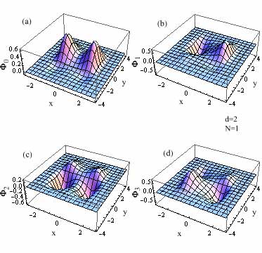
Eigenvalues EΞΊsubscriptπΈπœ…E_{\kappa} (ΞΊ=0βˆ’3πœ…03\kappa=0-3) for d=2𝑑2d=2 with m=1.0π‘š1.0m=1.0 and Ξ±=10.0𝛼10.0\alpha=10.0 are plotted as a function of c𝑐c in Fig. 3(b). An energy gap between the ground and first-excited states is Ξ©1=0.08630subscriptΞ©10.08630\Omega_{1}=0.08630 and 0.029890.029890.02989 for c=0.0𝑐0.0c=0.0 and 1.01.01.0, respectively. The c𝑐c dependence of eigenvalues for a quadratic coupling is similar to that for a linear coupling shown in Fig. 3(a). Figures 8(a)-8(d) show eigenfunctions of Φκ​(x,y)subscriptΞ¦πœ…π‘₯𝑦\Phi_{\kappa}(x,y) (ΞΊ=0βˆ’3πœ…03\kappa=0-3).

Refer to caption
Figure 8: (Color online) Eigenfunctions of (a) Ξ¦0​(x,y)subscriptΞ¦0π‘₯𝑦\Phi_{0}(x,y), (b) Ξ¦1​(x,y)subscriptΞ¦1π‘₯𝑦\Phi_{1}(x,y), (c) Ξ¦2​(x,y)subscriptΞ¦2π‘₯𝑦\Phi_{2}(x,y), and (d) Ξ¦3​(x,y)subscriptΞ¦3π‘₯𝑦\Phi_{3}(x,y) for the quadratic coupling (d=2𝑑2d=2) for a quadratic coupling (d=2𝑑2d=2) (m=1.0π‘š1.0m=1.0, Ξ±=10.0𝛼10.0\alpha=10.0, c=1.0𝑐1.0c=1.0 and N=1𝑁1N=1).
Refer to caption
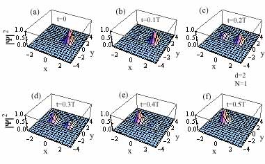
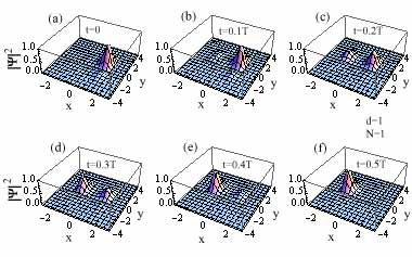
Figure 9: (Color online) |Ψ​(x,y,t)|2superscriptΞ¨π‘₯𝑦𝑑2|\Psi(x,y,t)|^{2} for a quadratic coupling (d=2𝑑2d=2) at (a) t=0.0𝑑0.0t=0.0, (b) t=0.1​T𝑑0.1𝑇t=0.1T, (c) t=0.2​T𝑑0.2𝑇t=0.2T, (d) t=0.3​T𝑑0.3𝑇t=0.3T, (e) t=0.4​T𝑑0.4𝑇t=0.4T and (f) t=0.5​T𝑑0.5𝑇t=0.5T where T=210.25𝑇210.25T=210.25 for a quadratic coupling (d=2𝑑2d=2) (m=1.0π‘š1.0m=1.0, Ξ±=10.0𝛼10.0\alpha=10.0, c=1.0𝑐1.0c=1.0 and N=1𝑁1N=1).

We consider a wavepacket Ψ​(x,y,t)Ξ¨π‘₯𝑦𝑑\Psi(x,y,t) given by Eq. (25). Figures 9(a)-9(f) show 3D plots of |Ψ​(x,y,t)|2superscriptΞ¨π‘₯𝑦𝑑2|\Psi(x,y,t)|^{2} at (a) T=0𝑇0T=0, (b) 0.1​T0.1𝑇0.1T, (c) 0.2​T0.2𝑇0.2T, (d) 0.3​T0.3𝑇0.3T, (e) 0.4​T0.4𝑇0.4T and (f) 0.5​T0.5𝑇0.5T where T=210.25𝑇210.25T=210.25. At t=0.0𝑑0.0t=0.0, a peak of the wavepacket locates at (xm,ym)=(1.2354,0.6468)subscriptπ‘₯π‘šsubscriptπ‘¦π‘š1.23540.6468(x_{m},y_{m})=(1.2354,0.6468). At t∼0.5​Tsimilar-to𝑑0.5𝑇t\sim 0.5\;T, wavepacket has appreciable magnitude at (x,y)=(βˆ’1.2354,0.6468)π‘₯𝑦1.23540.6468(x,y)=(-1.2354,0.6468) because the minimum of the composite potential U​(x,y)π‘ˆπ‘₯𝑦U(x,y) locates at (x,y)=(βˆ’1.4120, 1.8959)π‘₯𝑦1.41201.8959(x,y)=(-1.4120,\;1.8959). The tunneling of the wavepacket occurs between (x,y)=(1.2354,0.6468)π‘₯𝑦1.23540.6468(x,y)=(1.2354,0.6468) and (βˆ’1.2354,0.6468)1.23540.6468(-1.2354,0.6468).

Refer to caption
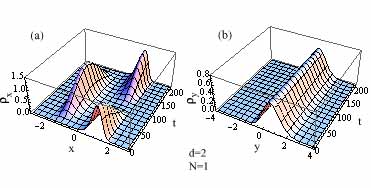
Figure 10: (Color online) Time dependence of (a) ρx​(t)subscript𝜌π‘₯𝑑\rho_{x}(t) and (b) ρy​(t)subscriptπœŒπ‘¦π‘‘\rho_{y}(t) for a quadratic coupling (d=2𝑑2d=2) (m=1.0π‘š1.0m=1.0, Ξ±=10.0𝛼10.0\alpha=10.0, c=1.0𝑐1.0c=1.0 and N=1𝑁1N=1).
Refer to caption
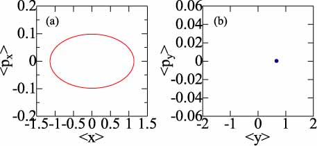
Figure 11: (Color online) Phase space representations of (a) ⟨px⟩delimited-⟨⟩subscript𝑝π‘₯\langle p_{x}\rangle vs. ⟨x⟩delimited-⟨⟩π‘₯\langle x\rangle and (b) ⟨py⟩delimited-⟨⟩subscript𝑝𝑦\langle p_{y}\rangle vs. ⟨y⟩delimited-βŸ¨βŸ©π‘¦\langle y\rangle for a quadratic coupling (d=2𝑑2d=2) (m=1.0π‘š1.0m=1.0, Ξ±=10.0𝛼10.0\alpha=10.0, c=1.0𝑐1.0c=1.0 and N=1𝑁1N=1).

By using Eqs. (25), (41)-(44), we may obtain marginal probability densities of xπ‘₯x and y𝑦y components, which are given by

ρx​(t)subscript𝜌π‘₯𝑑\displaystyle\rho_{x}(t) =\displaystyle= 12​[Ο•0​(x)2+Ο•1​(x)2]+cos⁑(ΞΈ1βˆ’ΞΈ2)​ϕ0​(x)​ϕ1​(x)​cos⁑Ω1​t,12delimited-[]subscriptitalic-Ο•0superscriptπ‘₯2subscriptitalic-Ο•1superscriptπ‘₯2subscriptπœƒ1subscriptπœƒ2subscriptitalic-Ο•0π‘₯subscriptitalic-Ο•1π‘₯subscriptΞ©1𝑑\displaystyle\frac{1}{2}\left[\phi_{0}(x)^{2}+\phi_{1}(x)^{2}\right]+\cos(\theta_{1}-\theta_{2})\>\phi_{0}(x)\phi_{1}(x)\>\cos\Omega_{1}t, (78)
ρy​(t)subscriptπœŒπ‘¦π‘‘\displaystyle\rho_{y}(t) =\displaystyle= 12​[(cos2⁑θ1+cos2⁑θ2)β€‹Οˆ0​(y)2+(sin2⁑θ1+sin2⁑θ2)β€‹Οˆ1​(y)2]12delimited-[]superscript2subscriptπœƒ1superscript2subscriptπœƒ2subscriptπœ“0superscript𝑦2superscript2subscriptπœƒ1superscript2subscriptπœƒ2subscriptπœ“1superscript𝑦2\displaystyle\frac{1}{2}\left[\left(\cos^{2}\theta_{1}+\cos^{2}\theta_{2}\right)\psi_{0}(y)^{2}+\left(\sin^{2}\theta_{1}+\sin^{2}\theta_{2}\right)\psi_{1}(y)^{2}\right] (79)
+\displaystyle+ 12​[sin⁑(2​θ1)+sin⁑(2​θ2)β€‹Οˆ0​(y)β€‹Οˆ1​(y)].12delimited-[]2subscriptπœƒ12subscriptπœƒ2subscriptπœ“0𝑦subscriptπœ“1𝑦\displaystyle\frac{1}{2}\left[\sin(2\theta_{1})+\sin(2\theta_{2})\psi_{0}(y)\psi_{1}(y)\right].

Figures 10(a) and 10(b) show ρx​(t)subscript𝜌π‘₯𝑑\rho_{x}(t) and ρy​(t)subscriptπœŒπ‘¦π‘‘\rho_{y}(t), respectively. ρx​(t)subscript𝜌π‘₯𝑑\rho_{x}(t) is similar to the relevant result for the linear coupling in Fig. 6(a) although ρy​(t)subscriptπœŒπ‘¦π‘‘\rho_{y}(t) is different from that in Fig. 6(b).

The tunneling probability Pr​(t)subscriptπ‘ƒπ‘Ÿπ‘‘P_{r}(t) is given by

Pr​(t)subscriptπ‘ƒπ‘Ÿπ‘‘\displaystyle P_{r}(t) =\displaystyle= 12βˆ’b​cos⁑(ΞΈ1βˆ’ΞΈ2)​cos⁑Ω1​t,12𝑏subscriptπœƒ1subscriptπœƒ2subscriptΞ©1𝑑\displaystyle\frac{1}{2}-b\cos{(\theta_{1}-\theta_{2})}\cos\Omega_{1}t, (80)

which is the same as Eq. (52) for a linear coupling.

Various time-dependent expectation values are given by

⟨x⟩delimited-⟨⟩π‘₯\displaystyle\langle x\rangle =\displaystyle= γ​cos⁑(ΞΈ1βˆ’ΞΈ2)​cos⁑Ω1​t,𝛾subscriptπœƒ1subscriptπœƒ2subscriptΞ©1𝑑\displaystyle\gamma\>\cos(\theta_{1}-\theta_{2})\>\cos\Omega_{1}t, (81)
⟨px⟩delimited-⟨⟩subscript𝑝π‘₯\displaystyle\langle p_{x}\rangle =\displaystyle= βˆ’Ξ·β€‹cos⁑(ΞΈ1βˆ’ΞΈ2)​sin⁑Ω1​t,πœ‚subscriptπœƒ1subscriptπœƒ2subscriptΞ©1𝑑\displaystyle-\eta\>\cos(\theta_{1}-\theta_{2})\>\sin\Omega_{1}t, (82)
⟨y⟩delimited-βŸ¨βŸ©π‘¦\displaystyle\langle y\rangle =\displaystyle= Ξ³y2​(sin⁑2​θ1+sin⁑2​θ2),subscript𝛾𝑦22subscriptπœƒ12subscriptπœƒ2\displaystyle\frac{\gamma_{y}}{2}\left(\>\sin 2\theta_{1}+\sin 2\theta_{2}\right), (83)
⟨py⟩delimited-⟨⟩subscript𝑝𝑦\displaystyle\langle p_{y}\rangle =\displaystyle= 0.0\displaystyle 0. (84)

Figures 11(a) and 11(b) show parametric plots of ⟨x⟩delimited-⟨⟩π‘₯\langle x\rangle vs. ⟨px⟩delimited-⟨⟩subscript𝑝π‘₯\langle p_{x}\rangle and ⟨y⟩delimited-βŸ¨βŸ©π‘¦\langle y\rangle vs. ⟨py⟩delimited-⟨⟩subscript𝑝𝑦\langle p_{y}\rangle, respectively. The former is ellipsoid while the latter is a point at (⟨y⟩,⟨py⟩)=(0.70186,0.0)delimited-βŸ¨βŸ©π‘¦delimited-⟨⟩subscript𝑝𝑦0.701860.0(\langle y\rangle,\langle p_{y}\rangle)=(0.70186,0.0) staying at the initial state. Although ⟨x⟩delimited-⟨⟩π‘₯\langle x\rangle vs. ⟨px⟩delimited-⟨⟩subscript𝑝π‘₯\langle p_{x}\rangle plot in Fig. 11(a) is similar to that for a linear coupling in Fig. 7(a), ⟨y⟩delimited-βŸ¨βŸ©π‘¦\langle y\rangle vs. ⟨py⟩delimited-⟨⟩subscript𝑝𝑦\langle p_{y}\rangle plot in Fig. 11(b) is quite different from that for a linear coupling in Fig. 7(b).
Refer to caption
Figure 12: (Color online) |Ψ​(x,y,t)|2superscriptΞ¨π‘₯𝑦𝑑2|\Psi(x,y,t)|^{2} of the four-component wavepacket given by Eq. (85) for a linear coupling (d=1𝑑1d=1) at (a) t=0.0𝑑0.0t=0.0, (b) t=0.1​T𝑑0.1𝑇t=0.1T, (c) t=0.2​T𝑑0.2𝑇t=0.2T, (d) t=0.3​T𝑑0.3𝑇t=0.3T, (e) t=0.4​T𝑑0.4𝑇t=0.4T and (f) t=0.5​T𝑑0.5𝑇t=0.5T where T=71.6084𝑇71.6084T=71.6084 (m=1.0π‘š1.0m=1.0, Ξ±=10.0𝛼10.0\alpha=10.0, c=0.1𝑐0.1c=0.1 and N=1𝑁1N=1).

IV Discussion

IV.1 A wavepacket with a0=a1=a2=a3=1/2subscriptπ‘Ž0subscriptπ‘Ž1subscriptπ‘Ž2subscriptπ‘Ž312a_{0}=a_{1}=a_{2}=a_{3}=1/2

In the preceding section, we consider a wavepacket with a0=a1=1/2subscriptπ‘Ž0subscriptπ‘Ž112a_{0}=a_{1}=1/\sqrt{2} and a2=a3=0.0subscriptπ‘Ž2subscriptπ‘Ž30.0a_{2}=a_{3}=0.0. Here we will study a four-component wavepacket with coefficients of a0=a1=a2=a3=1/2subscriptπ‘Ž0subscriptπ‘Ž1subscriptπ‘Ž2subscriptπ‘Ž312a_{0}=a_{1}=a_{2}=a_{3}=1/2 in Eq. (23)

Ψ​(x,y,t)Ξ¨π‘₯𝑦𝑑\displaystyle\Psi(x,y,t) =\displaystyle= 12β€‹βˆ‘ΞΊ=03Φκ​(x,y)​eβˆ’i​Eκ​t/ℏ.12superscriptsubscriptπœ…03subscriptΞ¦πœ…π‘₯𝑦superscript𝑒𝑖subscriptπΈπœ…π‘‘Planck-constant-over-2-pi\displaystyle\frac{1}{2}\sum_{\kappa=0}^{3}\;\Phi_{\kappa}(x,y)\>e^{-iE_{\kappa}t/\hbar}. (85)

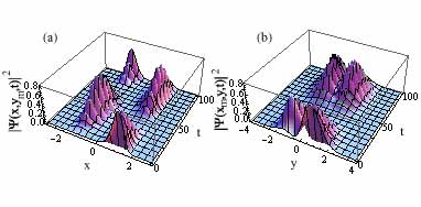
For a linear coupling (d=1𝑑1d=1) with c=0.1𝑐0.1c=0.1, m=1.0π‘š1.0m=1.0, Ξ±=10.0𝛼10.0\alpha=10.0 and N=1𝑁1N=1, we obtain eigenvalues of (E0,E1,E2,E3)=(βˆ’4.30784,βˆ’4.22313,βˆ’3.42868,βˆ’3.34397)subscript𝐸0subscript𝐸1subscript𝐸2subscript𝐸34.307844.223133.428683.34397(E_{0},E_{1},E_{2},E_{3})=(-4.30784,-4.22313,-3.42868,-3.34397). The peak of the wavepacket initially locates at (x,y)=(xm,ym)=(1.2353,β€…0.80775)π‘₯𝑦subscriptπ‘₯π‘šsubscriptπ‘¦π‘š1.23530.80775(x,y)=(x_{m},y_{m})=(1.2353,\>0.80775). The time-dependence of |Ψ​(x,y,t)|2superscriptΞ¨π‘₯𝑦𝑑2|\Psi(x,y,t)|^{2} from t=0𝑑0t=0 to t=T/2𝑑𝑇2t=T/2 are shown in Fig. 12 where T=71.6084𝑇71.6084T=71.6084 (below). With time developing, a new peak appears at (x,y)β‰ (xm,ym)π‘₯𝑦subscriptπ‘₯π‘šsubscriptπ‘¦π‘š(x,y)\neq(x_{m},y_{m}), and at t=T𝑑𝑇t=T wavepacket returns to its initial position.
Refer to caption
Figure 13: (Color online) (a) 3D plots of |Ψ​(x,ym,t)|2superscriptΞ¨π‘₯subscriptπ‘¦π‘šπ‘‘2|\Psi(x,y_{m},t)|^{2} with ym=0.761169subscriptπ‘¦π‘š0.761169y_{m}=0.761169 and (b) |Ψ​(xm,y,t)|2superscriptΞ¨subscriptπ‘₯π‘šπ‘¦π‘‘2|\Psi(x_{m},y,t)|^{2} with xm=1.23534subscriptπ‘₯π‘š1.23534x_{m}=1.23534 of the wavepacket given by Eq. (85) (m=1.0π‘š1.0m=1.0, Ξ±=10.0𝛼10.0\alpha=10.0, c=0.1𝑐0.1c=0.1, d=1𝑑1d=1 and N=1𝑁1N=1).
Refer to caption
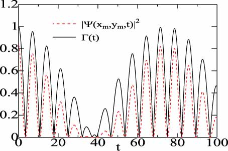
Figure 14: (Color online) Time dependence of Γ​(t)Γ𝑑\Gamma(t) (solid curve) and |Ψ​(xm,ym,t)|2superscriptΞ¨subscriptπ‘₯π‘šsubscriptπ‘¦π‘šπ‘‘2|\Psi(x_{m},y_{m},t)|^{2} (dashed curve) with (xm,ym)=(1.23534,β€…0.761169)subscriptπ‘₯π‘šsubscriptπ‘¦π‘š1.235340.761169(x_{m},y_{m})=(1.23534,\>0.761169) for the wavepacket given by Eq. (85) (m=1.0π‘š1.0m=1.0, Ξ±=10.0𝛼10.0\alpha=10.0, c=0.1𝑐0.1c=0.1, d=1𝑑1d=1 and N=1𝑁1N=1).

Calculations of ρx​(t)subscript𝜌π‘₯𝑑\rho_{x}(t) and ρy​(t)subscriptπœŒπ‘¦π‘‘\rho_{y}(t) for this wavepacket consisting of four terms are very tedious though it is not impossible. As their substitutes, we show the 3D plot of |Ψ​(x,ym,t)|2superscriptΞ¨π‘₯subscriptπ‘¦π‘šπ‘‘2|\Psi(x,y_{m},t)|^{2} as functions of xπ‘₯x and t𝑑t in Fig. 13(a), and that of |Ψ​(xm,y,t)|2superscriptΞ¨subscriptπ‘₯π‘šπ‘¦π‘‘2|\Psi(x_{m},y,t)|^{2} as functions of y𝑦y and t𝑑t in Fig. 13(b). Both |Ψ​(x,ym,t)|2superscriptΞ¨π‘₯subscriptπ‘¦π‘šπ‘‘2|\Psi(x,y_{m},t)|^{2} and |Ψ​(xm,y,t)|2superscriptΞ¨subscriptπ‘₯π‘šπ‘¦π‘‘2|\Psi(x_{m},y,t)|^{2} show complicated and rapid oscillations. The dashed curve in Fig. 14 expresses |Ψ​(xm,ym,t)|2superscriptΞ¨subscriptπ‘₯π‘šsubscriptπ‘¦π‘šπ‘‘2|\Psi(x_{m},y_{m},t)|^{2} as a function of t𝑑t, and the solid curve shows the correlation function Γ​(t)Γ𝑑\Gamma(t) defined by

Γ​(t)Γ𝑑\displaystyle\Gamma(t) =\displaystyle= |βˆ«βˆ’βˆžβˆžβˆ«βˆ’βˆžβˆžΞ¨βˆ—β€‹(x,y,0)​Ψ​(x,y,t)​𝑑x​𝑑y|,superscriptsubscriptsuperscriptsubscriptsuperscriptΞ¨π‘₯𝑦0Ξ¨π‘₯𝑦𝑑differential-dπ‘₯differential-d𝑦\displaystyle|\int_{-\infty}^{\infty}\int_{-\infty}^{\infty}\>\Psi^{*}(x,y,0)\>\Psi(x,y,t)\;dxdy\>|, (86)
=\displaystyle= 14|1+eβˆ’i​Ω1​t+eβˆ’i​Ω2​t+eβˆ’i​Ω3​t|.Β (Ωκ=(EΞΊβˆ’E0)/ℏ)\displaystyle\frac{1}{4}|1+\>e^{-i\Omega_{1}t}+e^{-i\Omega_{2}t}+e^{-i\Omega_{3}t}|.\hskip 28.45274pt\mbox{ ($\Omega_{\kappa}=(E_{\kappa}-E_{0})/\hbar)$} (87)

From the condition for the tunneling period T𝑇T,

T=minβˆ€t>0⁑{Γ​(t)=1},𝑇subscriptfor-all𝑑0Γ𝑑1\displaystyle T=\min_{\forall\>t\>>0}\;\large\{\Gamma(t)=1\large\}, (88)

we obtain T=71.6084𝑇71.6084T=71.6084 which is slightly different from a value estimated by 2​π/(E1βˆ’E0)=74.17062πœ‹subscript𝐸1subscript𝐸074.17062\pi/(E_{1}-E_{0})=74.1706. Although the tunneling period is mainly determined by E0subscript𝐸0E_{0} and E1subscript𝐸1E_{1}, its precise value is influenced by contributions from higher exited states with E2subscript𝐸2E_{2} and E3subscript𝐸3E_{3}.

IV.2 Coupling dependence of T𝑇T for other choices of parameters of mπ‘šm and α𝛼\alpha

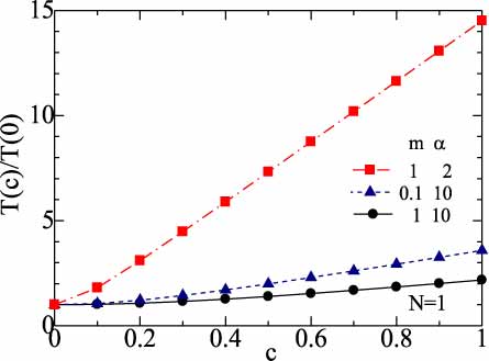
We have so far presented model calculations with a set of parameters of (m,Ξ±)=(1.0,10.0)π‘šπ›Ό1.010.0(m,\alpha)=(1.0,10.0) with c=1.0𝑐1.0c=1.0 and N=1𝑁1N=1. We have calculated the tunneling period T𝑇T as a function of the interaction c𝑐c for three sets of parameters: (m,Ξ±)=(1.0,10.0)π‘šπ›Ό1.010.0(m,\alpha)=(1.0,10.0), (0.1,10.0)0.110.0(0.1,10.0) and (1.0,2.0)1.02.0(1.0,2.0), whose results are shown in Fig. 15. We note that T𝑇T is increased with increasing c𝑐c, which is more significant for smaller mπ‘šm and for smaller α𝛼\alpha.

Refer to caption
Figure 15: (Color online) The c𝑐c dependence of the tunneling period T𝑇T for three sets of parameters of (m,Ξ±)=(1.0,10.0)π‘šπ›Ό1.010.0(m,\alpha)=(1.0,10.0) (solid curve), (0.1,10.0)0.110.0(0.1,10.0) (dashed curve) and (1.0,2.0)1.02.0(1.0,2.0) (chain curve) with N=1𝑁1N=1.

IV.3 The case of N>1𝑁1N>1

In the case of N>1𝑁1N>1, we have to numerically evaluate eigenvalues and eigenfunctions of the energy matrix with dimension of (Nm+1)Γ—(Nm+1)subscriptπ‘π‘š1subscriptπ‘π‘š1(N_{m}+1)\times(N_{m}+1) by using MATHEMATICA, where Nm+1=2​(N+1)subscriptπ‘π‘š12𝑁1N_{m}+1=2(N+1). Since we have neglected excited states higher than Ο΅2subscriptitalic-Ο΅2\epsilon_{2} of DW system, a reasonable choice of N𝑁N for the maximum quantum state of HO is expected to be given by

(N+12)β€‹β„β€‹Ο‰βˆΌ(Ο΅2βˆ’Ο΅0)=3.4641.similar-to𝑁12Planck-constant-over-2-piπœ”subscriptitalic-Ο΅2subscriptitalic-Ο΅03.4641\displaystyle\left(N+\frac{1}{2}\right)\>\hbar\omega\sim(\epsilon_{2}-\epsilon_{0})=3.4641. (89)

By using Eqs. (27) and (89), we obtain N∼3.5similar-to𝑁3.5N\sim 3.5 for Ξ±=10.0𝛼10.0\alpha=10.0 and N∼19.6similar-to𝑁19.6N\sim 19.6 for Ξ±=2.0𝛼2.0\alpha=2.0.

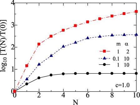
N𝑁N dependences of the tunneling period T𝑇T calculated for three sets of parameters: (m,Ξ±)=(1.0,10.0)π‘šπ›Ό1.010.0(m,\alpha)=(1.0,10.0), (0.1,10.0)0.110.0(0.1,10.0) and (1.0,2.0)1.02.0(1.0,2.0) with c=1.0𝑐1.0c=1.0 are shown in Fig. 16 where the ordinate is in the logarithmic scale. It is noted that T𝑇T is significantly increased with increasing N𝑁N, in particular for smaller mπ‘šm and smaller α𝛼\alpha. In the case of (m,Ξ±)=(1.0,10.0)π‘šπ›Ό1.010.0(m,\alpha)=(1.0,10.0), the enhancement of T𝑇T saturates at N≳4greater-than-or-equivalent-to𝑁4N\gtrsim 4. On the contrary, such a saturation is not realized in the case of (m,Ξ±)=(1.0,2.0)π‘šπ›Ό1.02.0(m,\alpha)=(1.0,2.0) even at N=10𝑁10N=10.

Refer to caption
Figure 16: (Color online) The N𝑁N dependence of the tunneling period T𝑇T for three sets of parameters of (m,Ξ±)=(1.0,10.0)π‘šπ›Ό1.010.0(m,\alpha)=(1.0,10.0) (solid curve), (0.1,10.0)0.110.0(0.1,10.0) (dashed curve) and (1.0,2.0)1.02.0(1.0,2.0) (chain curve) for a linear coupling (d=1𝑑1d=1) with c=1.0𝑐1.0c=1.0. Results of N=0𝑁0N=0 stand for those of no couplings.

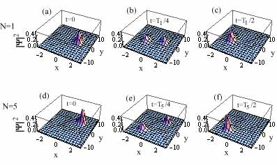
Paying attention to the case of (m,Ξ±)=(1.0,2.0)π‘šπ›Ό1.02.0(m,\alpha)=(1.0,2.0) which shows the most significant N𝑁N dependence of T𝑇T in Fig. 16, we have calculated the time-dependent wavepackets for N=1𝑁1N=1 and 555, whose results are shown in Fig. 17. We obtain Ξ©1=0.594662Γ—10βˆ’3subscriptΞ©10.594662superscript103\Omega_{1}=0.594662\times 10^{-3} for N=1𝑁1N=1, and Ξ©1=0.923365Γ—10βˆ’4subscriptΞ©10.923365superscript104\Omega_{1}=0.923365\times 10^{-4} for N=5𝑁5N=5. The initial position of wavepacket for N=1𝑁1N=1 is (x,y)=(1.23526,1.66213)π‘₯𝑦1.235261.66213(x,y)=(1.23526,1.66213), while that for N=5𝑁5N=5 is (x,y)=(1.23532,5.54669)π‘₯𝑦1.235325.54669(x,y)=(1.23532,5.54669). Figure 17(a)-17(c) show magnitudes of wavepackets at 0.0≀t≀T1/20.0𝑑subscript𝑇120.0\leq t\leq T_{1}/2 where T1(=1056.6)annotatedsubscript𝑇1absent1056.6T_{1}\;(=1056.6) denotes the tunneling period for N=1𝑁1N=1. Figure 17(d)-17(f) show similar results at 0.0≀t≀T5/20.0𝑑subscript𝑇520.0\leq t\leq T_{5}/2 where the tunneling period for N=5𝑁5N=5 is T5=68046.6subscript𝑇568046.6T_{5}=68046.6. Comparing time-dependent magnitudes of wavepackets in Figs. 17(a)-17(c) for N=1𝑁1N=1 with those in Fig. 17(d)-17(f) for N=5𝑁5N=5, we note that two results are similar when reading them by the normalized time t/T𝑑𝑇t/T, despite the fact that the tunneling period T5subscript𝑇5T_{5} is larger than T1subscript𝑇1T_{1} by a factor of 64.4.

Refer to caption
Figure 17: (Color online) |Ψ​(x,y,t)|2superscriptΞ¨π‘₯𝑦𝑑2|\Psi(x,y,t)|^{2} with N=1𝑁1N=1 at (a) t=0.0𝑑0.0t=0.0, (b) t=T1/4𝑑subscript𝑇14t=T_{1}/4 and (c) t=T1/2𝑑subscript𝑇12t=T_{1}/2 where T1=1056.6subscript𝑇11056.6T_{1}=1056.6; |Ψ​(x,y,t)|2superscriptΞ¨π‘₯𝑦𝑑2|\Psi(x,y,t)|^{2} with N=5𝑁5N=5 at (d) t=0.0𝑑0.0t=0.0, (e) t=T5/4𝑑subscript𝑇54t=T_{5}/4 and (f) t=T5/2𝑑subscript𝑇52t=T_{5}/2 where T5=68046.6subscript𝑇568046.6T_{5}=68046.6 (d=1𝑑1d=1, m=1.0π‘š1.0m=1.0, Ξ±=2.0𝛼2.0\alpha=2.0 and c=1.0𝑐1.0c=1.0).

IV.4 Uncertainty relation

The Heisenberg uncertainty of Δ​x​Δ​pxΞ”π‘₯Ξ”subscript𝑝π‘₯\Delta x\Delta p_{x}, which is also a typical quantum phenomenon, is related with the tunneling Hasegawa13 . We may obtain analytical expressions for averages of fluctuations of xπ‘₯x and pxsubscript𝑝π‘₯p_{x} in the case of N=1𝑁1N=1. For a linear coupling, we obtain

(Δ​x)2superscriptΞ”π‘₯2\displaystyle(\Delta x)^{2} =\displaystyle= ⟨x2βŸ©βˆ’βŸ¨x⟩2,delimited-⟨⟩superscriptπ‘₯2superscriptdelimited-⟨⟩π‘₯2\displaystyle\langle x^{2}\rangle-\langle x\rangle^{2}, (90)
=\displaystyle= Ξ³02​(cos2⁑θ1+sin2⁑θ2)+Ξ³12​(sin2⁑θ1+cos2⁑θ2)βˆ’Ξ³2​cos2⁑(ΞΈ1βˆ’ΞΈ2)​cos2⁑Ω1​t,subscript𝛾02superscript2subscriptπœƒ1superscript2subscriptπœƒ2subscript𝛾12superscript2subscriptπœƒ1superscript2subscriptπœƒ2superscript𝛾2superscript2subscriptπœƒ1subscriptπœƒ2superscript2subscriptΞ©1𝑑\displaystyle\frac{\gamma_{0}}{2}(\cos^{2}\theta_{1}+\sin^{2}\theta_{2})+\frac{\gamma_{1}}{2}(\sin^{2}\theta_{1}+\cos^{2}\theta_{2})-\gamma^{2}\cos^{2}(\theta_{1}-\theta_{2})\;\cos^{2}\Omega_{1}t, (91)
(Δ​px)2superscriptΞ”subscript𝑝π‘₯2\displaystyle(\Delta p_{x})^{2} =\displaystyle= ⟨px2βŸ©βˆ’βŸ¨px⟩2,delimited-⟨⟩superscriptsubscript𝑝π‘₯2superscriptdelimited-⟨⟩subscript𝑝π‘₯2\displaystyle\langle p_{x}^{2}\rangle-\langle p_{x}\rangle^{2}, (92)
=\displaystyle= Ο‡02​(cos2⁑θ1+sin2⁑θ2)+Ο‡12​(sin2⁑θ1+cos2⁑θ2)βˆ’Ξ·2​cos2⁑(ΞΈ1+ΞΈ2)​sin2⁑Ω1​t,subscriptπœ’02superscript2subscriptπœƒ1superscript2subscriptπœƒ2subscriptπœ’12superscript2subscriptπœƒ1superscript2subscriptπœƒ2superscriptπœ‚2superscript2subscriptπœƒ1subscriptπœƒ2superscript2subscriptΞ©1𝑑\displaystyle\frac{\chi_{0}}{2}(\cos^{2}\theta_{1}+\sin^{2}\theta_{2})+\frac{\chi_{1}}{2}(\sin^{2}\theta_{1}+\cos^{2}\theta_{2})-\eta^{2}\cos^{2}(\theta_{1}+\theta_{2})\;\sin^{2}\Omega_{1}t, (93)

with

Ο‡0subscriptπœ’0\displaystyle\chi_{0} =\displaystyle= βˆ«βˆ’βˆžβˆž[βˆ‚xΟ•0​(x)]2​𝑑x=2.58707,superscriptsubscriptsuperscriptdelimited-[]subscriptπ‘₯subscriptitalic-Ο•0π‘₯2differential-dπ‘₯2.58707\displaystyle\int_{-\infty}^{\infty}\>[\partial_{x}\phi_{0}(x)]^{2}\>dx=2.58707, (94)
Ο‡1subscriptπœ’1\displaystyle\chi_{1} =\displaystyle= βˆ«βˆ’βˆžβˆž[βˆ‚xΟ•1​(x)]2​𝑑x=3.17399,superscriptsubscriptsuperscriptdelimited-[]subscriptπ‘₯subscriptitalic-Ο•1π‘₯2differential-dπ‘₯3.17399\displaystyle\int_{-\infty}^{\infty}\>[\partial_{x}\phi_{1}(x)]^{2}\>dx=3.17399, (95)

where ΞΈ1subscriptπœƒ1\theta_{1} and ΞΈ2subscriptπœƒ2\theta_{2} are given by Eqs. (45) and (46), respectively. For a quadratic coupling, they are given by

(Δ​x)2superscriptΞ”π‘₯2\displaystyle(\Delta x)^{2} =\displaystyle= Ξ³02+Ξ³12βˆ’Ξ³2​cos2⁑(ΞΈ1βˆ’ΞΈ2)​cos2⁑Ω1​t,subscript𝛾02subscript𝛾12superscript𝛾2superscript2subscriptπœƒ1subscriptπœƒ2superscript2subscriptΞ©1𝑑\displaystyle\frac{\gamma_{0}}{2}+\frac{\gamma_{1}}{2}-\gamma^{2}\cos^{2}(\theta_{1}-\theta_{2})\;\cos^{2}\Omega_{1}t, (96)
(Δ​px)2superscriptΞ”subscript𝑝π‘₯2\displaystyle(\Delta p_{x})^{2} =\displaystyle= Ο‡02+Ο‡12βˆ’Ξ·2​cos2⁑(ΞΈ1βˆ’ΞΈ2)​sin2⁑Ω1​t,subscriptπœ’02subscriptπœ’12superscriptπœ‚2superscript2subscriptπœƒ1subscriptπœƒ2superscript2subscriptΞ©1𝑑\displaystyle\frac{\chi_{0}}{2}+\frac{\chi_{1}}{2}-\eta^{2}\cos^{2}(\theta_{1}-\theta_{2})\;\sin^{2}\Omega_{1}t, (97)

where ΞΈ1subscriptπœƒ1\theta_{1} and ΞΈ2subscriptπœƒ2\theta_{2} are given by Eqs. (76) and (77), respectively. For uncoupled DW (c=0.0𝑐0.0c=0.0) where ΞΈ1=ΞΈ2=0subscriptπœƒ1subscriptπœƒ20\theta_{1}=\theta_{2}=0, Eqs. (91) and (93) reduce to

(Δ​x)2superscriptΞ”π‘₯2\displaystyle(\Delta x)^{2} =\displaystyle= Ξ³02+Ξ³12βˆ’Ξ³2​cos2⁑Ω1​t,subscript𝛾02subscript𝛾12superscript𝛾2superscript2subscriptΞ©1𝑑\displaystyle\frac{\gamma_{0}}{2}+\frac{\gamma_{1}}{2}-\gamma^{2}\;\cos^{2}\Omega_{1}t, (98)
(Δ​px)2superscriptΞ”subscript𝑝π‘₯2\displaystyle(\Delta p_{x})^{2} =\displaystyle= Ο‡02+Ο‡12βˆ’Ξ·2​sin2⁑Ω1​t.subscriptπœ’02subscriptπœ’12superscriptπœ‚2superscript2subscriptΞ©1𝑑\displaystyle\frac{\chi_{0}}{2}+\frac{\chi_{1}}{2}-\eta^{2}\;\sin^{2}\Omega_{1}t. (99)

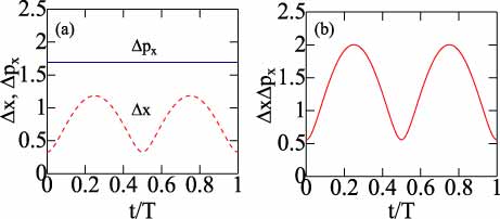
Figure 18(a) shows time dependences of Δ​xΞ”π‘₯\Delta x and Δ​pxΞ”subscript𝑝π‘₯\Delta p_{x} for a linear coupling with m=1.0π‘š1.0m=1.0, Ξ±=10.0𝛼10.0\alpha=10.0, c=1.0𝑐1.0c=1.0 and N=1𝑁1N=1. Although Δ​xΞ”π‘₯\Delta x oscillates with an appreciable magnitude of Ξ³2superscript𝛾2\gamma^{2} in Eq. (91), Δ​pxΞ”subscript𝑝π‘₯\Delta p_{x} is almost constant (≃1.69similar-to-or-equalsabsent1.69\simeq 1.69) because of a small Ξ·2superscriptπœ‚2\eta^{2} in Eq. (93). Figure 18(b) shows the uncertainty given by Δ​x​Δ​pxΞ”π‘₯Ξ”subscript𝑝π‘₯\Delta x\Delta p_{x}, which is initially 0.5568750.5568750.556875. The Heisenberg uncertainty relation: Δ​x​Δ​pxβ‰₯ℏ/2Ξ”π‘₯Ξ”subscript𝑝π‘₯Planck-constant-over-2-pi2\Delta x\Delta p_{x}\geq\hbar/2 is always preserved. We note that Δ​x​Δ​pxΞ”π‘₯Ξ”subscript𝑝π‘₯\Delta x\Delta p_{x} has a large magnitude at t∼T/4similar-to𝑑𝑇4t\sim T/4 or 3​T/43𝑇43T/4 when tunneling takes place (Fig. 5). This shows that the uncertainty is related with quantum tunneling Hasegawa13 .
Refer to caption
Figure 18: (Color online) (a) Time dependences of Δ​xΞ”π‘₯\Delta x (dashed curve) and Δ​pxΞ”subscript𝑝π‘₯\Delta p_{x} (solid curve), and (b) the uncertainty: Δ​x​Δ​pxΞ”π‘₯Ξ”subscript𝑝π‘₯\Delta x\Delta p_{x} for a linear coupling (m=1.0π‘š1.0m=1.0, Ξ±=1.0𝛼1.0\alpha=1.0, c=1.0𝑐1.0c=1.0 and N=1𝑁1N=1).

V Concluding remark

We have studied wavepacket dynamics in the Razavy hyperbolic DW potential Razavy80 which is coupled to a HO by linear and quadratic interactions. Wavepackets show the quantum tunneling between two bottoms in the composite potential U​(x,y)π‘ˆπ‘₯𝑦U(x,y) [Eq. (31)]. The tunneling period is increased with increasing c𝑐c and/or N𝑁N, which is more significant for smaller mπ‘šm and smaller α𝛼\alpha (Figs. 15 and 16). Comparing results of linear and quadratic couplings, we note that the tunneling probability Pr​(t)subscriptπ‘ƒπ‘Ÿπ‘‘P_{r}(t) is the same and the marginal probability density ρx​(t)subscript𝜌π‘₯𝑑\rho_{x}(t) is similar between the two, but ρy​(t)subscriptπœŒπ‘¦π‘‘\rho_{y}(t) is different (Figs. 6 and 10). Furthermore, ⟨y⟩delimited-βŸ¨βŸ©π‘¦\langle y\rangle vs. ⟨py⟩delimited-⟨⟩subscript𝑝𝑦\langle p_{y}\rangle plot in the quadratic coupling stay at the initial position in the phase space, while that in the linear coupling shows an elliptic motion (Figs. 7 and 11). Our phase space plots of ⟨x⟩delimited-⟨⟩π‘₯\langle x\rangle vs. ⟨px⟩delimited-⟨⟩subscript𝑝π‘₯\langle p_{x}\rangle and ⟨y⟩delimited-βŸ¨βŸ©π‘¦\langle y\rangle vs. ⟨py⟩delimited-⟨⟩subscript𝑝𝑦\langle p_{y}\rangle for the two-term wavepacket given by Eq. (25) are quite different from relevant results obtained in Babyuk02 , where trajectories show ellipse-like orbits but they do not return to initial positions after revolution in a quartic DW potential coupled to HO (see Figs. 4.2 and 4.5 in Babyuk02 ). Ref. Babyuk02 showed that this oddity occurs even for uncoupled DW (see Fig. 3.2 in Babyuk02 ), for which our calculation leads to the complete elliptic trajectory for ⟨x⟩delimited-⟨⟩π‘₯\langle x\rangle vs. ⟨px⟩delimited-⟨⟩subscript𝑝π‘₯\langle p_{x}\rangle plot because we obtain

⟨x⟩delimited-⟨⟩π‘₯\displaystyle\langle x\rangle =\displaystyle= γ​cos⁑Ω1​t,⟨px⟩=βˆ’Ξ·β€‹sin⁑Ω1​t,𝛾subscriptΞ©1𝑑delimited-⟨⟩subscript𝑝π‘₯πœ‚subscriptΞ©1𝑑\displaystyle\gamma\>\cos\Omega_{1}t,\;\;\;\langle p_{x}\rangle=-\eta\>\sin\Omega_{1}t, (100)

for c=0.0𝑐0.0c=0.0 in Eqs. (55) and (57). This difference between the result of Ref.Babyuk02 and ours does not arise from the difference between quartic and hyperbolic DW potentials, because a chain of equations of motion for expectation values in a general symmetric DW potential is closed within ⟨x⟩delimited-⟨⟩π‘₯\langle x\rangle and ⟨px⟩delimited-⟨⟩subscript𝑝π‘₯\langle p_{x}\rangle for the two-term wavepacket (see the Appendix). It has been shown that the uncertainty of Δ​x​Δ​pxΞ”π‘₯Ξ”subscript𝑝π‘₯\Delta x\Delta p_{x} becomes appreciable when the tunneling takes place (Fig. 18). It would be interesting to experimentally observed |Ψ​(x,t)|2superscriptΞ¨π‘₯𝑑2|\Psi(x,t)|^{2} and Δ​x​Δ​pxΞ”π‘₯Ξ”subscript𝑝π‘₯\Delta x\Delta p_{x}, which might be possible with advanced recent technology.

Acknowledgements.
This work is partly supported by a Grant-in-Aid for Scientific Research from Ministry of Education, Culture, Sports, Science and Technology of Japan.

*

Appendix A Expectation values for the two-term wavepacket

A coupled DW system is assumed to be described by the Hamiltonian given by

H=px22​M+py22​m+U​(x,y),𝐻superscriptsubscript𝑝π‘₯22𝑀superscriptsubscript𝑝𝑦22π‘šπ‘ˆπ‘₯𝑦\displaystyle H=\frac{p_{x}^{2}}{2M}+\frac{p_{y}^{2}}{2m}+U(x,y), (A1)

with

U​(x,y)π‘ˆπ‘₯𝑦\displaystyle U(x,y) =\displaystyle= V​(x)+m​ω2​y22βˆ’c​xd​y,𝑉π‘₯π‘šsuperscriptπœ”2superscript𝑦22𝑐superscriptπ‘₯𝑑𝑦\displaystyle V(x)+\frac{m\omega^{2}y^{2}}{2}-c\>x^{d}\>y, (A2)

where V​(x)𝑉π‘₯V(x) denotes a general symmetric DW potential and d=1𝑑1d=1 (d=2𝑑2d=2) signifies a linear (quadratic) coupling. We consider the two-term wavepacket given by

Ψ​(x,y,t)Ξ¨π‘₯𝑦𝑑\displaystyle\Psi(x,y,t) =\displaystyle= 12​[Ξ¦0​(x,y)​eβˆ’i​E0​t/ℏ+Ξ¦1​(x,y)​eβˆ’i​E1​t/ℏ],12delimited-[]subscriptΞ¦0π‘₯𝑦superscript𝑒𝑖subscript𝐸0𝑑Planck-constant-over-2-pisubscriptΞ¦1π‘₯𝑦superscript𝑒𝑖subscript𝐸1𝑑Planck-constant-over-2-pi\displaystyle\frac{1}{\sqrt{2}}\large[\Phi_{0}(x,y)\>e^{-iE_{0}t/\hbar}+\Phi_{1}(x,y)\>e^{-iE_{1}t/\hbar}\large], (A3)

where real eigenfunctions of Ξ¦0​(x,y)subscriptΞ¦0π‘₯𝑦\Phi_{0}(x,y) and Ξ¦1​(x,y)subscriptΞ¦1π‘₯𝑦\Phi_{1}(x,y) satisfy the SchΓΆdinger equation

H​Φ0​(x,y)𝐻subscriptΞ¦0π‘₯𝑦\displaystyle H\Phi_{0}(x,y) =\displaystyle= E0​Φ0​(x,y),subscript𝐸0subscriptΞ¦0π‘₯𝑦\displaystyle E_{0}\Phi_{0}(x,y), (A4)
H​Φ1​(x,y)𝐻subscriptΞ¦1π‘₯𝑦\displaystyle H\Phi_{1}(x,y) =\displaystyle= E1​Φ1​(x,y)=(E0+Ξ©1)​Φ1​(x,y).subscript𝐸1subscriptΞ¦1π‘₯𝑦subscript𝐸0subscriptΞ©1subscriptΞ¦1π‘₯𝑦\displaystyle E_{1}\Phi_{1}(x,y)=(E_{0}+\Omega_{1})\Phi_{1}(x,y). (A5)

Expectation values of ⟨x⟩delimited-⟨⟩π‘₯\langle x\rangle and ⟨px⟩delimited-⟨⟩subscript𝑝π‘₯\langle p_{x}\rangle for the wavepacket are expressed by

⟨x⟩delimited-⟨⟩π‘₯\displaystyle\langle x\rangle =\displaystyle= ax​cos⁑Ω1​t,subscriptπ‘Žπ‘₯subscriptΞ©1𝑑\displaystyle a_{x}\>\cos\Omega_{1}t, (A6)
⟨px⟩delimited-⟨⟩subscript𝑝π‘₯\displaystyle\langle p_{x}\rangle =\displaystyle= βˆ’bx​sin⁑Ω1​t,subscript𝑏π‘₯subscriptΞ©1𝑑\displaystyle-b_{x}\>\sin\Omega_{1}t, (A7)

where

axsubscriptπ‘Žπ‘₯\displaystyle a_{x} =\displaystyle= ∫∫Φ0​(x,y)​x​Φ1​(x,y)​𝑑x​𝑑y,subscriptΞ¦0π‘₯𝑦π‘₯subscriptΞ¦1π‘₯𝑦differential-dπ‘₯differential-d𝑦\displaystyle\int\int\>\Phi_{0}(x,y)\>x\>\Phi_{1}(x,y)\>dxdy, (A8)
bxsubscript𝑏π‘₯\displaystyle b_{x} =\displaystyle= ∫∫Φ0​(x,y)​(βˆ’iβ€‹βˆ‚x)​Φ1​(x,y)​𝑑x​𝑑y.subscriptΞ¦0π‘₯𝑦𝑖subscriptπ‘₯subscriptΞ¦1π‘₯𝑦differential-dπ‘₯differential-d𝑦\displaystyle\int\int\>\Phi_{0}(x,y)\>(-i\partial_{x})\Phi_{1}(x,y)\>dxdy. (A9)

Equations (A6) and (A7) lead to

dβ€‹βŸ¨x⟩d​t𝑑delimited-⟨⟩π‘₯𝑑𝑑\displaystyle\frac{d\langle x\rangle}{dt} =\displaystyle= βˆ’Ξ©1​ax​sin⁑Ω1​t=(Ξ©1​axbx)β€‹βŸ¨px⟩,subscriptΞ©1subscriptπ‘Žπ‘₯subscriptΞ©1𝑑subscriptΞ©1subscriptπ‘Žπ‘₯subscript𝑏π‘₯delimited-⟨⟩subscript𝑝π‘₯\displaystyle-\Omega_{1}a_{x}\>\sin\Omega_{1}t=\left(\frac{\Omega_{1}a_{x}}{b_{x}}\right)\langle p_{x}\rangle, (A10)
dβ€‹βŸ¨px⟩d​t𝑑delimited-⟨⟩subscript𝑝π‘₯𝑑𝑑\displaystyle\frac{d\langle p_{x}\rangle}{dt} =\displaystyle= βˆ’Ξ©1​bx​cos⁑Ω1​t=βˆ’(Ξ©1​bxax)β€‹βŸ¨x⟩.subscriptΞ©1subscript𝑏π‘₯subscriptΞ©1𝑑subscriptΞ©1subscript𝑏π‘₯subscriptπ‘Žπ‘₯delimited-⟨⟩π‘₯\displaystyle-\Omega_{1}b_{x}\>\cos\Omega_{1}t=-\left(\frac{\Omega_{1}b_{x}}{a_{x}}\right)\langle x\rangle. (A11)

On the other hand, Heisenberg equations of motion for xπ‘₯x and pxsubscript𝑝π‘₯p_{x} are given by

d​xd​t𝑑π‘₯𝑑𝑑\displaystyle\frac{dx}{dt} =\displaystyle= βˆ‚Hβˆ‚px=pxM,𝐻subscript𝑝π‘₯subscript𝑝π‘₯𝑀\displaystyle\frac{\partial H}{\partial p_{x}}=\frac{p_{x}}{M}, (A12)
d​pxd​t𝑑subscript𝑝π‘₯𝑑𝑑\displaystyle\frac{dp_{x}}{dt} =\displaystyle= βˆ’βˆ‚Hβˆ‚x=βˆ’βˆ‚xU​(x,y).𝐻π‘₯subscriptπ‘₯π‘ˆπ‘₯𝑦\displaystyle-\frac{\partial H}{\partial x}=-\partial_{x}U(x,y). (A13)

Taking averages of Eqs. (A12) and (A13) over the two-term wavepacket Ψ​(x,y,t)Ξ¨π‘₯𝑦𝑑\Psi(x,y,t) given by Eq. (A3), we obtain

dβ€‹βŸ¨x⟩d​t𝑑delimited-⟨⟩π‘₯𝑑𝑑\displaystyle\frac{d\langle x\rangle}{dt} =\displaystyle= βˆ’1Mβ€‹βˆ«βˆ«Ξ¦0​(x,y)β€‹βˆ‚xΞ¦1​(x,y)​d​x​d​y​sin⁑Ω1​t,1𝑀subscriptΞ¦0π‘₯𝑦subscriptπ‘₯subscriptΞ¦1π‘₯𝑦𝑑π‘₯𝑑𝑦subscriptΞ©1𝑑\displaystyle-\frac{1}{M}\int\int\Phi_{0}(x,y)\>\partial_{x}\Phi_{1}(x,y)\>dxdy\>\sin\Omega_{1}t, (A14)
dβ€‹βŸ¨px⟩d​t𝑑delimited-⟨⟩subscript𝑝π‘₯𝑑𝑑\displaystyle\frac{d\langle p_{x}\rangle}{dt} =\displaystyle= βˆ’βˆ«βˆ«Ξ¦0​(x,y)β€‹βˆ‚xU​(x,y)​Φ1​(x,y)​d​x​d​y​cos⁑Ω1​t.subscriptΞ¦0π‘₯𝑦subscriptπ‘₯π‘ˆπ‘₯𝑦subscriptΞ¦1π‘₯𝑦𝑑π‘₯𝑑𝑦subscriptΞ©1𝑑\displaystyle-\int\int\Phi_{0}(x,y)\>\partial_{x}U(x,y)\>\Phi_{1}(x,y)\>dxdy\>\cos\Omega_{1}t. (A15)

The equivalence of Eqs. (A10) and (A11) with Eqs. (A14) and (A15), respectively, may be shown as follows: Multiplying Eqs. (A4) and (A5) by x​Φ1​(x,y)π‘₯subscriptΞ¦1π‘₯𝑦x\>\Phi_{1}(x,y) and integrating them over xπ‘₯x and y𝑦y with integrations by parts, we obtain

Ξ©1​axsubscriptΞ©1subscriptπ‘Žπ‘₯\displaystyle\Omega_{1}a_{x} =\displaystyle= 1Mβ€‹βˆ«βˆ«Ξ¦0​(x,y)β€‹βˆ‚xΞ¦1​(x,y)​d​x​d​y.1𝑀subscriptΞ¦0π‘₯𝑦subscriptπ‘₯subscriptΞ¦1π‘₯𝑦𝑑π‘₯𝑑𝑦\displaystyle\frac{1}{M}\int\int\Phi_{0}(x,y)\>\partial_{x}\Phi_{1}(x,y)\>dxdy. (A16)

Multiplications of Eqs. (A4) and (A5) by βˆ‚xΞ¦1​(x,y)subscriptπ‘₯subscriptΞ¦1π‘₯𝑦\partial_{x}\Phi_{1}(x,y) and integrations of them over xπ‘₯x and y𝑦y lead to

Ξ©1​bxsubscriptΞ©1subscript𝑏π‘₯\displaystyle\Omega_{1}b_{x} =\displaystyle= ∫∫Φ0​(x)β€‹βˆ‚xU​(x,y)​Φ1​(x,y)​d​x​d​y.subscriptΞ¦0π‘₯subscriptπ‘₯π‘ˆπ‘₯𝑦subscriptΞ¦1π‘₯𝑦𝑑π‘₯𝑑𝑦\displaystyle\int\int\Phi_{0}(x)\>\partial_{x}U(x,y)\>\Phi_{1}(x,y)\>dxdy. (A17)

It is well known that Heisenberg equations of motion given by Eqs. (A12) and (A13) generally yield a hierarchical chain for DW potentials. Fortunately, equations of motion for expectation values for the two-term wavepacket close within ⟨x⟩delimited-⟨⟩π‘₯\langle x\rangle and ⟨px⟩delimited-⟨⟩subscript𝑝π‘₯\langle p_{x}\rangle as given by Eqs. (A10) and (A11). Such a simplification does not occur for a general wavepacket, as given by Eqs. (23) and (24).

Similar calculations may be made also for ⟨y⟩delimited-βŸ¨βŸ©π‘¦\langle y\rangle and ⟨py⟩delimited-⟨⟩subscript𝑝𝑦\langle p_{y}\rangle. Then both the ⟨x⟩delimited-⟨⟩π‘₯\langle x\rangle vs. ⟨px⟩delimited-⟨⟩subscript𝑝π‘₯\langle p_{x}\rangle plot and the ⟨y⟩delimited-βŸ¨βŸ©π‘¦\langle y\rangle vs. ⟨py⟩delimited-⟨⟩subscript𝑝𝑦\langle p_{y}\rangle plot are elliptic for the two-term wavepacket.

References

  • (1) D. J. Tannor, Introduction to quantum mechanics: A time-dependent perspective (Univ. Sci. Books, Sausalito, California, 2007).
  • (2) K. M. Christoffel and J. M. Bowman, J. Chem Phys. 74 (1981) 5057.
  • (3) N. Makri and W. Miller, J. Chem Phys. 87 (1987) 5781.
  • (4) R. P. Feymann and A. R. Hibbs, Quantum mechanics and path integrals (McGraw-Hill, New York, 2005).
  • (5) D. Babyuk, arXiv:0208070.
  • (6) M. Razavy, Am. J. Phys. 48 (1980) 285.
  • (7) F. Finkel, arXiv:9905020.
  • (8) B. Bagchi and A. Ganguly, arXiv:0302040.
  • (9) H. Hasegawa, arXiv:1403.0543.
  • (10) H. Hasegawa, Physica A 392 (2013) 6232.