Handling convexity-like constraints in variational problems

Abstract.

We provide a general framework to construct finite dimensional approximations of the space of convex functions, which also applies to the space of $c$-convex functions and to the space of support functions of convex bodies. We give precise estimates of the distance between the approximation space and the admissible set. This framework applies to the approximation of convex functions by piecewise linear functions on a mesh of the domain and by other finite-dimensional spaces such as tensor-product splines. We show how these discretizations are well suited for the numerical solution of problems of calculus of variations under convexity constraints. Our implementation relies on proximal algorithms, and can be easily parallelized, thus making it applicable to large scale problems in dimension two and three. We illustrate the versatility and the efficiency of our approach on the numerical solution of three problems in calculus of variation : 3D denoising, the principal agent problem, and optimization within the class of convex bodies.

1. Introduction

Several problems in the calculus of variations come with natural convexity constraints. In optimal transport, Brenier theorem asserts that every optimal transport plan can be written as the gradient of a convex function, when the cost is the squared Euclidean distance. Jordan, Kinderlehrer and Otto showed [9] that some evolutionary PDEs such as the Fokker-Planck equation can be reformulated as a gradient flow of a functional in the space of probability densities endowed with the natural distance constructed from optimal transport, namely the Wasserstein space. In the corresponding time-discretized schemes, each timestep involves the solution of a convex optimization problem over the set of gradient of convex functions. In a different context, the principal agent problem proposed by Rochet and Choné [22] in economy also comes with natural convexity constraints. Despite the possible applications, the numerical implementation of these variational problems has been lagging behind, mainly because of a non-density phenomenon discovered by Choné and Le Meur [5].

Figure 1. Illustration of the non-density result phenomena of Choné and Le Meur on the grid $G_{\delta}$ (top left). We consider the convex function $f(x,y)=\max(0,x+y-1)$ on $[0,1]^{2}$ and its projection $g$ on the intersection $\mathcal{H}_{M_{\varepsilon}}\cap E_{\delta}$, where $E_{\delta}$ is the space of piecewise linear functions on $G_{\delta}$ and $\mathcal{H}_{M_{\varepsilon}}$ is the space of function satisfying the relaxed convexity constraints of Definition 2.1. The error $\left|f-g\right|$ is displayed for three different choices of grid size, and $\varepsilon\ll\delta$. One can observe that the maximum error $\left\|f-g\right\|_{\infty}$ remains almost constant regardless of $\delta$. (In all figures, the upper left and lower right corners corresponds to the value $0.2$.)

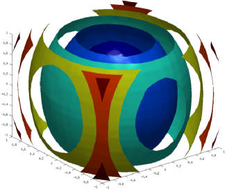
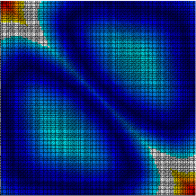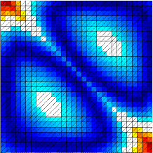
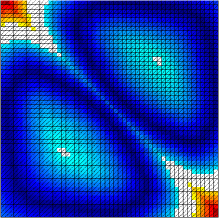
Choné and Le Meur discovered that some convex functions cannot be approximated by piecewise-linear convex functions on a regular grid (such as the grid displayed in Figure 1). More precisely, they proved that piecewise-linear convex functions on the regular grid automatically satisfy the inequality $\frac{\partial^{2}f}{\partial x\partial y}\geqslant 0$ in a the sense of distributions. Since there exists convex functions that do not satisfy this inequality, this implies that the union of the spaces of piecewise-linear convex functions on the regular grids $(G_{\delta})_{\delta>0}$ is not dense in the space of convex functions on the unit square. Moreover, this difficulty is local, and it is likely that for any fixed sequence of meshes, one can construct convex functions $f$ that cannot be obtained as limits of piecewise-linear convex functions on these meshes. This phenomenon makes it challenging to use P¹ finite elements to approximate the solution of variational problems with convexity constraints.

1.1. Related works

In this section, we briefly discuss approaches that have been proposed in the last decade to tackle the problem discovered by Choné and Le Meur.

Mesh versus grid constraints

Carlier, Lachand-Robert and Maury proposed in [4] to replace the space of P¹ convex functions by the space of the space of convex interpolates. For every fixed mesh, a piecewise linear function is a convex interpolate if it is obtained by linearly interpolating the restriction of a convex function to the node of the mesh. Note that these functions are not necessarily convex, and the method is therefore not interior. Density results are straightforward in this context but the number of linear constraints which have to be imposed on nodes values is rather large. The authors observe that in the case of a regular grid, one needs $\simeq m^{1.8}$ constraints in order to describe the space of convex interpolates, where $m$ stands for the number of nodes of the mesh.

Aguilera and Morin [1] proposed a finite-difference approximation of the space of convex functions using discrete convex Hessians. They prove that it is possible to impose convexity by requiring a linear number of nonlinear constraints with respect to the number of nodes. The leading fully nonlinear optimization problems are solved using semidefinite programming codes. Whereas, convergence is proved in a rather general setting, the practical efficiency of this approach is limited by the capability of semidefinite solvers. In a similar spirit, Oberman [18] considers the space of function that satisfy local convexity constraints on a finite set of directions. By changing the size of the stencil, the author proposed different discretizations which lead to exterior or interior approximations. Estimates of the quality of the approximation are given for smooth convex functions.

Higher order approximation by convex tensor-product splines

An important number of publications have been dedicated in recent years to solve shape preserving least square problems. For instance, different sufficient conditions have been introduced to force the convexity of the approximating functions. Whereas this problem is well understood in dimension one, it is still an active field of research in the context of multivariate polynomials like Bézier or tensor spline functions. We refer the reader to Jüttler [10] and references therein for a detailed description of recent results. In this article, Jüttler describes an interior discretization of convex tensor-product splines. This approach is based on the so called “Blossoming theory” which makes it possible to linearize constraints on the Hessian matrix by introducing additional variables. Based on this framework, the author illustrates the method by computing the $L^{2}$ projection of some given function into the space of convex tensor-product splines. Two major difficulties have to be pointed out. First, the density of convex tensor splines in the space of convex functions is absolutely non trivial, and one may expect phenomena similar to those discovered by Choné and Le Meur. Second, the proposed algorithm leads to a very large number of linear constraints.

Dual approaches

Lachand-Robert and Oudet [12] developed a strategy related to the dual representation of a convex body by its support functions. They rely on a simple projection approach that amounts to the computation of a convex hull, thus avoiding the need to describe the constraints defining the set of support functions. To the best of our knowledge, this article is the first one to attack the question of solving problems of calculus of variations within convex bodies. The resulting algorithm can be interpreted as a non-smooth projected gradient descent, and gave interesting results on difficult problems such as Newton’s or Alexandrov’s problems. In a similar geometric framework, Oudet studied in [20] approximations of convex bodies based on Minkowski sums. It is well known in dimension two that every convex polygon can be decomposed as a finite sum of segments and triangles. While this result cannot be generalized to higher dimension, this approach still allows the generation of random convex polytopes. This process was used by the author to study numerically two problems of calculus of variations on the space of convex bodies with additional width constraints.

Ekeland and Moreno-Bromberg [6] proposed a dual approach for parameterizing the space of convex functions on a domain. Given a finite set of points $S$ in the domain, they parameterize convex functions by their value $f_{s}$ and their gradient $v_{s}$ at those points. In order to ensure that these couples of values and gradients $(f_{s},v_{s})_{s\in S}$ are induced by a convex function, they add for every pair of points in $S$ the constraints $f_{t}\geqslant f_{s}+\langle t-s|v_{s}\rangle$. This discretization is interior, and it is easy to show that the phenomenon of Choné and Le Meur does not occur for this type of approximation. However, the high number of constraints makes it difficult to solve large-scale problems using this approach. Mirebeau [17] is currently investigating an adaptative version of this method that would allow its application to larger problems.

1.2. Contributions

We provide a general framework to construct approximations of the space of convex functions on a bounded domain that satisfies a Lipschitz bound. Our approximating space is a finite-dimensional polyhedron, that is a subset of a finite-dimensional functional space that satisfies a finite number of linear constraints. The main theoretical contribution of this article is a bound on the (Hausdorff) distance between the approximating polyhedron and the admissible set of convex functions, which is summarized in Theorem 2.5. This bound implies in particular the density of the discretized space of functions in the space of convex functions. Our discretization is not specific to approximation by piecewise linear functions on a triangulation of the domain, and can easily be extended to approximations of convex functions within other finite-dimensional subspaces, such as the space of tensor product splines. This is illustrated numerically in Section 6.

This type of discretization is well suited to the numerical solution of problems of calculus of variations under convexity constraints. For instance, we show how to compute the $\mathrm{L}^{2}$ projection onto the discretized space of convex functions in dimension $d=2,3$ by combining a proximal algorithm [2] and an efficient projection operator on the space of $1$D discrete convex functions. Because of the structure of the problem, these $1$D projection steps can be performed in parallel, thus making our approach applicable to large scale problems in higher dimension. We apply our non-smooth approach to a denoising problem in dimension three in Section 5. Other problems of calculus of variations under convexity constraints, such as the principal-agent problem, can be solved using variants of this algorithm. This aspect is illustrated in Section 6.

Finally, we note in Section 3 that the discretization of the space of convex functions we propose can be generalized to other spaces of functions satisfying similar constraints, such as the space of support functions of convex bodies. The proximal algorithm can also be applied to this modified case, thus providing the first method able to approximate the projection of a function on the sphere onto the space of support functions of convex bodies. Section 7 presents numerical computations of $\mathrm{L}^{p}$ projections (for $p=1,2,\infty$) of the support function of a unit regular simplex onto the set of support functions of convex bodies with constant width. We believe that these projection operators could be useful in the numerical study of a famous conjecture due to Bonnesen and Fenchel (1934) concerning Meissner’s convex bodies.

Acknowledgements

The first named author would like to thank Robert McCann for introducing him to the principal-agent problem and Young-Heon Kim for interesting discussions. The authors would like to acknowledge the support of the French Agence National de la Recherche under references ANR-11-BS01-014-01 (TOMMI) and ANR-12-BS01-0007 (Optiform).

Notation

Given a metric space $X$, we denote $\mathcal{C}(X)$ the space of bounded continuous functions on $X$ endowed with the norm of uniform convergence $\left\|.\right\|_{\infty}$. Every subset $L$ of the space of affine forms on $\mathcal{C}(X)$ defines a convex subset $\mathcal{H}_{L}$ of the space of continuous functions by duality, denoted by:

$$\mathcal{H}_{L}:=\{g\in\mathcal{C}(K);~{}\forall\ell\in L,~{}\ell(g)\leqslant 0\}.$$ (1.1)

2. A relaxation framework for convexity

In this section, we concentrate on the relaxation of the standard convexity constraints for clarity of exposition. Most of the propositions presented below can be extended to the the generalizations of convexity presented in Section 3. Let $X$ be a bounded convex domain of $\mathbb{R}^{d}$, and let $\mathcal{H}$ be the set of continuous convex functions on $X$. We define $L_{k}$ as the set of linear forms $\ell$ on $\mathcal{C}(K)$ which can be written as

$$\ell(g)=g\left(\sum_{i=1}^{k}\lambda_{i}x_{i}\right)-\left(\sum_{i=1}^{k}\lambda_{i}g(x_{i})\right),$$ (2.2)

where $x_{1},\ldots,x_{k}$ are $k$ distinct points chosen in $X$, and where $(\lambda_{i})_{1\leqslant i\leqslant k}$ belongs to the $(k-1)$-dimensional simplex $\Delta^{k-1}$. In other words, $\lambda_{1},\ldots,\lambda_{k}$ are non-negative numbers whose sum is equal to one. Since we are only considering continuous functions, $\mathcal{H}_{L_{k}}$ and $\mathcal{H}$ coincide as soon as $k\geqslant 2$.

We introduce in Definition 2.1 below a discretization $M_{\varepsilon}$ of the set of convexity constraints $L_{2}$. Choné and Le Meur proved in [5] that the union of the spaces of piecewise-linear convex functions on regular grids of the square is not dense in the space of convex functions on this domain. This means that we need to be very careful in order to apply the convexity constraints $M_{\varepsilon}$ to finite-dimensional spaces of functions. If one considers the space $E_{\delta}$ of piecewise-linear functions on a triangulation of the domain with edgelengths bounded by $\delta$, then $\mathcal{H}_{M_{\varepsilon}}\cap E_{\delta}=\mathcal{H}\cap E_{\delta}$ as soon as $\varepsilon\ll\delta$. In this case, one can fall in the pitfall identified by Choné and Le Meur, as illustrated in Figure 1. Our goal in this section is to show that it is possible to choose $\varepsilon$ as a function of $\delta$ so that $\mathcal{H}_{M_{\varepsilon}}\cap E_{\delta}$ becomes dense in $\mathcal{H}$ as $\delta$ goes to zero. Before stating our main theorem, we need to introduce some definitions.

Figure 2. (Left) The discretized convexity constraints are enforced on the discrete segments $c_{pq}$ joining pairs of points of an $\varepsilon$-sampling of the boundary $U_{\varepsilon}\subseteq\partial X$. (Right) A triangulation of the domain $X$, which can be used to define a finite-dimensional subspace $E_{\delta}$ of continuous piecewise-linear functions on $X$. Note that $\varepsilon$ must be greater than $\delta$. The relation between the parameters $\delta$ and $\varepsilon$ is studied in Theorems 2.1–2.5.

Definition 2.1 (Discretized convexity constraints).

Given any triple of points $(x,y,z)$ in $X$ such that $z$ belongs to $[x,y]$, we define a linear form $\ell_{xyz}$ by

$$\ell_{xyz}(g):=g(z)-\frac{\left\|zy\right\|}{\left\|xy\right\|}g(x)-\frac{\left\|xz\right\|}{\left\|xy\right\|}g(x).$$ (2.3)

Here and below, we set $\left\|xy\right\|:=\left\|x-y\right\|$ to emphasize the notion of distance between $x$ and $y$. By convention, when we write $\ell_{xyz}$, we implicitly assume that $z$ lies on the segment $[x,y]$. Consider a subset $U_{\varepsilon}\subseteq\partial X$ such that for every point $x$ in $\partial X$ there exists a point $x_{\varepsilon}$ in $U_{\varepsilon}$ with $\left\|x-x_{\varepsilon}\right\|\leqslant\varepsilon$ (see Figure 2). Given any pair of distinct points $(p,q)$ in $U_{\varepsilon}$, we let $c_{pq}$ be the discrete segment defined by

$$c_{pq}:=\left\{p+\varepsilon i\frac{(q-p)}{\left\|q-p\right\|};i\in\mathbb{N},\,0\leqslant i\leqslant\left\|q-p\right\|/\varepsilon\right\}.$$

Finally, we define the following discretized set of constraints

$$M_{\varepsilon}:=\left\{\ell_{xyz};~{}x,y,z\in c_{pq}\hbox{ for some }p,q\in U_{\varepsilon}\hbox{ and }z\in[x,y]\right\}.$$ (2.4)

Definition 2.2 (Interpolation operator).

A (linear) interpolation operator is a continuous linear map $\mathcal{I}_{\delta}$ from the space $\mathcal{C}(X)$ to a finite-dimensional linear subspace $E_{\delta}\subseteq\mathcal{C}(X)$, whose restriction to $E_{\delta}$ is the identity map. We assume that the space $E_{\delta}$ contains the affine functions on $X$, and that the linear interpolation operator $I_{\delta}$ satisfies these properties:

$$\mathrm{Lip}(\mathcal{I}_{\delta}f) \leqslant C_{I}\mathrm{Lip}f$$ (L1)

$$\left\|f-\mathcal{I}_{\delta}f\right\|_{\infty} \leqslant\delta\mathrm{Lip}(f),$$ (L2)

$$\left\|f-\mathcal{I}_{\delta}f\right\|_{\infty} \leqslant\frac{1}{2}\delta^{2}\mathrm{Lip}(\nabla f),$$ (L3)

In practice, we consider families of linear interpolation operators parameterized by $\delta$, and we assume that $C_{I}\geqslant 1$ is constant for the whole family.

Example 2.1.

Consider a triangulation of a polyhedral domain $X$, such that each triangle has diameter at most $\delta$. Define $E_{\delta}$ as the space of functions that are linear on the triangles of the mesh, and $\mathcal{I}_{\delta}(f)$ as the linear interpolation of $f$ on the mesh. Then $(E_{\delta},I_{\delta})$ is an interpolation operator and satisfies (L1)–(L3). Other interpolation operators can be derived from higher-order finite elements, tensor-product splines, etc.

Definition 2.3 (Superior limit of sets).

The superior limit of a sequence of subsets $(A_{n})$ of $\mathcal{C}(X)$ is defined by

$$\overline{\lim}_{n\to\infty}A_{n}:=\{f\in\mathcal{C}(X);\exists f_{n}\in A_{n},s.t.\lim_{n\to\infty}f_{n}=f\}.$$

The following theorem shows that the non-density phenomenom identified by Choné and Le Meur doesn’t occur when $\varepsilon$ is chosen large enough, as a function of $\delta$. This theorem is a corollary of the more quantitative Theorem 2.5. The remainder of this section is devoted to the proof of Theorem 2.5.

Theorem 2.1.

Let $X$ be a bounded convex domain $X$ and $(I_{\delta})_{\delta>0}$ be a family of linear interpolation operators. Let $f$ be a function from $\mathbb{R}_{+}$ to $\mathbb{R}_{+}$ s.t.

$$\lim_{\delta\to 0}f(\delta)=0\qquad\lim_{\delta\to 0}\delta/f(\delta)^{2}=0.$$

We let $\mathrm{B}_{\mathrm{Lip}}^{\gamma}$ denotes the set of $\gamma$-Lipschitz functions on $X$. Then,

$$\mathcal{H}\cap\mathrm{B}_{\mathrm{Lip}}^{\gamma/C_{I}}\subseteq\left[\overline{\lim}_{\delta\to 0}\mathcal{H}_{M_{f(\delta)}}\cap\mathrm{B}_{\mathrm{Lip}}^{\gamma}\right]\subseteq\mathcal{H}\cap\mathrm{B}_{\mathrm{Lip}}^{\gamma}.$$ (2.5)

2.1. Relaxation of convexity constraints

The first step needed to prove Theorem 2.1 is to show that every function that belong to the space $\mathcal{H}_{M_{\varepsilon}}$ is close to a convex function on $X$ for the norm $\left\|.\right\|_{\infty}$. This result follows from an explicit upper bound on the distance between any function in $\mathcal{H}_{M_{\varepsilon}}$ and its convex envelope.

Definition 2.4 (Convex envelope).

Given a function $g$ on $X$, we define its convex envelope $\overline{g}$ by the following formula:

$$\overline{g}(x):=\min\left\{\sum_{i=1}^{d+1}\lambda_{i}g(x_{i});~{}x_{i}\in X,\lambda\in\Delta^{d}\hbox{ and }\sum_{i}\lambda_{i}x_{i}=x\right\},$$ (2.6)

where $\Delta^{d}$ denotes the $d$-simplex, i.e. $\lambda\in\mathbb{R}_{+}^{d+1}$ and $\sum\lambda_{i}=1$. The function $\overline{g}$ is convex and by construction, its graph lies below the graph of $g$.

Proposition 2.2.

For any function $g$ in the space $\mathcal{H}_{M_{\varepsilon}}$, the distance between $g$ and its convex envelope $\overline{g}$ is bounded by $\left\|g-\overline{g}\right\|_{\infty}\leqslant\mathrm{const}(d)\mathrm{Lip}(g)\varepsilon$.

This proposition follows from a more general result concerning a certain type of relaxation of convexity constraints, which we call $\alpha$-relaxation.

Definition 2.5 ($\alpha$-Relaxation).

Let $M,L$ be two sets of affine forms on the space $\mathcal{C}(X)$. The set $M$ is called an $\alpha$-relaxation of $L$, where $\alpha$ is a function from $\mathcal{C}(X)$ to $\mathbb{R}_{+}\cup\{+\infty\},$ if the following inequality holds:

$$\forall\ell\in L,\forall g\in\mathcal{C}(K),~{}\exists\ell_{g}\in M,~{}\left|\ell(g)-\ell_{g}(g)\right|\leqslant\alpha(g).$$ (2.7)

Proposition 2.3.

Consider an $\alpha$-relaxation $M$ of $L_{2}$. If $g$ lies in $\mathcal{H}_{M}$, the distance between $g$ and its convex envelope $\overline{g}$ is bounded by $\left\|g-\overline{g}\right\|_{\infty}\leqslant d\alpha(g)$.

Proof.

Let us show first that, assuming that $g$ is in $\mathcal{H}_{M}$, the following inequality holds for any form $\ell$ in $L_{k}$:

$$\ell(g)\leqslant k\alpha(g).$$ (2.8)

For $k=2$, this follows at once from our hypothesis. Indeed, there must exist a linear form $\ell_{g}$ in $M$ that satisfies (2.7), so that $\ell(g)\leqslant\ell_{g}(g)+\alpha(g)$. Since $g$ lies in $\mathcal{H}_{M}$, $\ell_{g}(g)$ is non-positive and we obtain (2.8). The case $k>2$ is proved by induction. Consider $\lambda$ in the simplex $\Delta^{k-1}$ and points $x_{1},\ldots,x_{k}$ in $X$. We assume $\lambda_{1}<1$ and we let $\mu_{i}=\lambda_{i}/(1-\lambda_{1})$ for any $i\geqslant 2$. The vector $\mu=(\mu_{2},\ldots,\mu_{k})$ lies in $\Delta^{k-2}$, and therefore $y=\sum_{i\geqslant 2}\mu_{i}x_{i}$ belongs to $X$. Applying the inductive hypothesis (2.8) twice, we obtain:

$$g\left(\lambda_{1}x_{1}+(1-\lambda_{1})y\right)-\left(\lambda_{1}g(x_{1})+(1-\lambda_{1})g\left(y\right)\right)\leqslant\alpha(g),$$

$$g(y)-\left(\sum_{i=2}^{k}\mu_{i}g(x_{i})\right)\leqslant(k-1)\alpha(g).$$

The sum of the first inequality and $(1-\lambda_{1})$ times the second one gives (2.8). Now, consider the convex envelope $\overline{g}$ of $g$. Given any family of points $(x_{i})$ and coefficients $(\lambda_{i})$ such that $\sum\lambda_{i}x_{i}=x$, we consider the form $\ell(f):=f(x)-\sum_{i}\lambda_{i}f(x_{i})$. Applying equation (2.8) to $\ell$ gives

$$g(x)-d\alpha(g)\leqslant\sum\lambda_{i}g(x_{i})$$

Taking the minimum over the $(x_{i})$, $(\lambda_{i})$ such that $\sum\lambda_{i}x_{i}=x$, we obtain the desired inequality $\left|g(x)-\overline{g}(x)\right|\leqslant d\alpha(g)$. ∎

In order to deduce Proposition 2.2 from Proposition 2.3, we should take $\alpha(g)$ proportional to $\mathrm{Lip}(g)$. We use a technical lemma that gives an upper bound on the difference between two linear forms corresponding to convexity constraints in term of $\mathrm{Lip}$.

Lemma 2.4.

Let $x,y,z$ and $x^{\prime},y^{\prime},z^{\prime}$ be six points in $X$. Assume the following

• $\max(\left\|x-x^{\prime}\right\|,\left\|y-y^{\prime}\right\|,\left\|z-z^{\prime}\right\|)\leqslant\eta$;

• $z\in[x,y]$, $z^{\prime}\in[x^{\prime},y^{\prime}]$.

Then, $\left|\ell_{xyz}(g)-\ell_{x^{\prime}y^{\prime}z^{\prime}}(g)\right|\leqslant 6\eta\mathrm{Lip}(g)$.

Proof.

We define $\lambda$ by the relation $z=\lambda x+(1-\lambda)y$, and $\lambda^{\prime}$ is defined similarly. We also define $\ell_{i}(g):=g(z)-(\lambda^{\prime}g(x)+(1-\lambda^{\prime})g(y))$. Then,

$$\left|\ell_{xyz}(g)-\ell_{x^{\prime}y^{\prime}z^{\prime}}(g)\right|\leqslant\left|\ell_{x^{\prime}y^{\prime}z}(g)-\ell_{i}(g)\right|+\left|\ell_{i}(g)-\ell_{xyz}(g)\right|$$

The first term is easily bounded by $2\eta\mathrm{Lip}(g)$, while the second term is bounded by $\left|\lambda-\lambda^{\prime}\right|\mathrm{Lip}(g)\left\|xy\right\|$.

$$\left|\lambda-\lambda^{\prime}\right| =\left|\frac{\left\|zy\right\|}{\left\|xy\right\|}-\frac{\left\|z^{\prime}y^{\prime}\right\|}{\left\|x^{\prime}y^{\prime}\right\|}\right|$$

$$\leqslant\left|\frac{\left\|zy\right\|-\left\|z^{\prime}y^{\prime}\right\|}{\left\|xy\right\|}\right|+\left|\frac{\left\|z^{\prime}y^{\prime}\right\|}{\left\|x^{\prime}y^{\prime}\right\|}\cdot\frac{\left\|x^{\prime}y^{\prime}\right\|-\left\|xy\right\|}{\left\|xy\right\|}\right|\leqslant 4\eta/\left\|xy\right\|$$

Overall, we get the desired upper bound.∎

Proof of Proposition 2.3.

Our goal is to show that $M_{\varepsilon}$ is an $\alpha$-relaxation of $L_{2}$. Consider three points $x,y,z$ in $X$ such that $z$ lies inside the segment $[x,y]$. The straight line $(x,y)$ intersects the boundary of $X$ in two points $a$ and $b$. By hypothesis, there exists two points $p$ and $q$ in $U_{\varepsilon}$ such that the distances $\left\|a-p\right\|$ and $\left\|b-q\right\|$ are bounded by $\varepsilon$. The maximum distance between the segments $[a,b]$ and $[p,q]$ is then also bounded by $\varepsilon$ and the maximum distance between the segment $[a,b]$ and the finite set $c_{pq}$ by $2\varepsilon$. This means that there exists three points $x_{\varepsilon},y_{\varepsilon}$ and $z_{\varepsilon}$ in $c_{pq}$ such that $\max(\left\|x-x_{\varepsilon}\right\|,\left\|y-y_{\varepsilon}\right\|,\left\|y-y_{\varepsilon}\right\|)\leqslant 2\varepsilon$. Using Lemma 2.4, we deduce that $\left\|\ell_{xyz}(g)-\ell_{x_{\varepsilon}y_{\varepsilon}z_{\varepsilon}}(g)\right\|\leqslant\alpha(g):=12\varepsilon\mathrm{Lip}(g)$. This implies that $M_{\varepsilon}$ is an $\alpha$-relaxation of $L_{2}$, and the statement follows from Proposition 2.3. ∎

2.2. Hausdorff approximation

In this section, we use the estimation of the previous paragraph to prove a quantitative version of Theorem 2.1, using the notion of directed Hausdorff distance.

Definition 2.6 (Hausdorff distances).

The directed or half-Hausdorff distance between two subsets $A,B$ of a $\mathcal{C}(X)$ is denoted $\mathrm{h}_{\mathrm{H}}(A|B)$:

$$\mathrm{h}_{\mathrm{H}}(A|B)=\min\left\{r\geqslant 0;\forall f\in A,~{}\exists g\in B,~{}\left\|f-g\right\|_{\infty}\leqslant r\right\}.$$ (2.9)

Note that this function is not symmetric in its argument.

Theorem 2.5.

Let $X$ be a bounded convex domain of $\mathbb{R}^{d}$ and $I_{\delta}:\mathcal{C}(X)\to E_{\delta}$ be interpolation operator satisfying (L1)–(L3). We let $\mathrm{B}_{\mathrm{Lip}}^{\gamma}$ be the set of $\gamma$-Lipschitz functions on $X$. Then, assuming $\gamma\geqslant 2C_{I}\operatorname{diam}(X)$,

$$\mathrm{h}_{\mathrm{H}}(\mathrm{B}_{\mathrm{Lip}}^{\gamma}\cap E_{\delta}\cap\mathcal{H}_{M_{\varepsilon}}\,|\,\mathrm{B}_{\mathrm{Lip}}^{\gamma}\cap\mathcal{H}) \leqslant\mathrm{const}(d)\gamma\varepsilon.$$ (2.10)

$$\mathrm{h}_{\mathrm{H}}(\mathrm{B}_{\mathrm{Lip}}^{\gamma/C_{I}}\cap\mathcal{H}\,|\,\mathrm{B}_{\mathrm{Lip}}^{\gamma}\cap E_{\delta}\cap\mathcal{H}_{M_{\varepsilon}}) \leqslant\mathrm{const}\frac{\gamma^{2}\delta}{\varepsilon^{2}}\operatorname{diam}(X),$$ (2.11)

Let $\mathrm{B}_{\mathcal{C}^{1,1}}^{\kappa}$ be the set of functions with $\kappa$-Lipschitz gradients ($\kappa\geqslant 1$). Then,

$$\mathrm{h}_{\mathrm{H}}(\mathrm{B}_{\mathcal{C}^{1,1}}^{\kappa}\cap\mathcal{H}\,|\,E_{\delta}\cap\mathcal{H}_{M_{\varepsilon}})\leqslant\mathrm{const}\cdot\kappa^{2}\operatorname{diam}(X)^{2}\frac{\delta^{2}}{\varepsilon^{2}}$$ (2.12)

Remark 2.1 (Choice of the parameter $\varepsilon$).

The previous theorem has implications on how to choose $\varepsilon$ as a function of $\delta$ in order to obtain theoretical convergence results. In practice, the estimations given by the items (i) and (ii) below seem to be rather pessimistic, and in applications we always choose $\varepsilon$ to be a small constant times $\delta$.

• If one chooses $\varepsilon=f(\delta)$, where $f$ is a function from $\mathbb{R}_{+}$ to $\mathbb{R}_{+}$ such that $\lim_{\delta\to 0}f(\delta)=0$ and $\lim_{\delta\to 0}\delta/f(\delta)^{2}=0$, the upper bounds in Equations (2.10)–(2.11) converges to zero when $\delta$ does. This implies the convergence result stated in Theorem 2.1.

• We can choose $\varepsilon$ so as to equate the two upper bound in Equations (2.10)–(2.11), i.e. $\varepsilon\simeq\delta^{1/3}$. This suggests that the best rate of convergence in Hausdorff distance that one can expect from this analysis, in order to recover all convex functions $\mathcal{H}\cap\mathrm{B}_{\mathrm{Lip}}^{\gamma}$, is in $\operatorname{O}(\delta^{1/3})$.

• On the other hand, Equation (2.12) shows that convex and $\mathcal{C}^{1,1}$ functions are easier to approximate by discrete convex functions. In particular, if $f$ is merely a superlinear function, i.e. $\lim_{\delta\to 0}f(\delta)=0$ and $\lim_{\delta\to 0}\delta/f(\delta)=0$, then, with $\varepsilon=f(\delta)$, the upper bounds of both Equation (2.10) and (2.12) converge to zero.

The following easy lemma shows that the space $\mathcal{H}_{M_{\varepsilon}}\cap E_{\delta}$ has non-empty interior for the topology induced by the finite-dimensional vector space $E_{\delta}$ as soon as $\delta<\varepsilon$. This very simple fact is the key to the proof of Theorem 2.5.

Lemma 2.6.

Consider the function $s(x):=\left\|x-x_{0}\right\|^{2}$ on $X$, where $x_{0}$ is a point in $X$, and the interpolating function $s_{\delta}:=\mathcal{I}_{\delta}s$. Then,

$$\max_{\ell\in M_{\varepsilon}}\ell(s_{\delta})\leqslant\delta^{2}-\varepsilon^{2}.$$

Proof.

Consider three points $x<z<y$ on the real line, such that $\left|x-z\right|\geqslant\varepsilon$ and $\left|y-z\right|\geqslant\varepsilon$ and $z=\lambda x+(1-\lambda)y$. Then,

$$z^{2}-\lambda x^{2}-(1-\lambda)y^{2} =z^{2}-\lambda(z+(x-z))^{2}-(1-\lambda)(z+(y-z))^{2}$$

$$=-[\lambda(x-z)^{2}+(1-\lambda)(y-z)^{2}]\leqslant-\varepsilon^{2}$$

Since the gradient of $s$ is $2$-Lipschitz, using (L3) we get $\left\|s-s_{\delta}\right\|_{\infty}\leqslant\delta^{2}$. Combining with the previous inequality, this implies $\ell(s_{\delta})\leqslant\delta^{2}-\varepsilon^{2}$ for every linear form $\ell$ in $M_{\varepsilon}$. ∎

Proof of Theorem 2.5.

Let $g$ be a function in the intersection $\mathcal{H}_{M_{\varepsilon}}\cap\mathrm{B}_{\mathrm{Lip}}^{\gamma}$. Then, Proposition 2.3 implies that its convex envelop $\overline{g}$ satisfies $\left\|g-\overline{g}\right\|_{\infty}\leqslant\mathrm{const}(d)\mathrm{Lip}(g)\varepsilon$. The Lipschitz constant of a function is not increased by taking its convex envelope, and thus $\overline{g}$ belongs to $\mathcal{H}\cap\mathrm{B}_{\mathrm{Lip}}^{\gamma}$. This implies the upper bound given in Equation (2.10).

On the other hand, given a convex function $f$ in $\mathcal{H}\cap\mathrm{B}_{\mathrm{Lip}}^{\gamma/C_{I}}$, we consider the function $g:=\mathcal{I}_{\delta}f$ defined by the interpolation operator. By property (L1) the function $g$ belongs to $\mathrm{B}_{\mathrm{Lip}}^{\gamma}$, and by property (L2) one has for any linear form $\ell$ in $L_{2}$,

$$\ell(g) =g(\lambda x+(1-\lambda)y)-(\lambda g(x)+(1-\lambda)g(y))$$

$$\leqslant f(\lambda x+(1-\lambda)y)-(\lambda f(x)+(1-\lambda)f(y))+2\delta\gamma\leqslant 2\delta\gamma$$

For $\eta<1$, we let $g_{\eta}:=(1-\eta)g+\eta s_{\delta}$. Assuming $\delta\leqslant\varepsilon/2$, the previous inequality implies that for any linear form $\ell$ in $M_{\varepsilon}$,

$$\ell(g_{\eta})\leqslant(1-\eta)2\delta\gamma+\eta(\delta^{2}-\varepsilon^{2})\leqslant 2\delta\gamma-\eta\varepsilon^{2}/2$$

Consequently, assuming $4\delta\gamma\leqslant\eta\varepsilon^{2}$ the inequality $\ell(g_{\eta})\leqslant 0$ holds for any linear form $\ell$ in $M_{\varepsilon}$, and $g$ belongs to $\mathcal{H}_{M_{\varepsilon}}$. Moreover, using the fact that $\mathrm{Lip}$ is a semi-norm, we have

$$\mathrm{Lip}(g_{\eta}) \leqslant(1-\eta)\mathrm{Lip}(g)+\eta\mathrm{Lip}(s_{\delta})$$

$$\leqslant(1-\eta)\gamma+2C_{I}\eta\operatorname{diam}(X)$$ (2.13)

In the second inequality, we used property (L1) and $\mathrm{Lip}(s)\leqslant 2\operatorname{diam}(X)$. By Equation 2.13, the function $g_{\eta}$ belongs to $\mathrm{B}_{\mathrm{Lip}}^{\gamma}$ provided that $\gamma\geqslant 2C_{I}\operatorname{diam}(X)$. From now on, we fix $\eta=4\delta\gamma/\varepsilon^{2}$, and let $h=g_{\eta}$, which by the discussion above belongs to $\mathcal{H}_{M_{\varepsilon}}\cap\mathrm{B}_{\mathrm{Lip}}^{\gamma}$. The distance between $f$ and $h$ is bounded by

$$\left\|f-h\right\|_{\infty}\leqslant\left\|f-g\right\|_{\infty}+\eta(\left\|g\right\|_{\infty}+\left\|s_{\delta}\right\|_{\infty}).$$

Since the space $E_{\delta}$ contains constant functions, we can assume that $\left\|g\right\|_{\infty}$ is bounded by $\mathrm{Lip}(g)\operatorname{diam}(X)\leqslant\gamma\operatorname{diam}(X)$. Assuming $\varepsilon\leqslant\operatorname{diam}(X)$,

$$\left\|f-h\right\|_{\infty}\leqslant\gamma\delta\left[1+\frac{4}{\varepsilon^{2}}\left(\gamma\operatorname{diam}(X)+\operatorname{diam}(X)^{2}\right)\right]\leqslant 10\frac{\gamma^{2}\delta}{\varepsilon^{2}}\operatorname{diam}(X),$$

thus implying Equation (2.11)

The proof of Equation (2.12) is very similar. Given a convex function $f$ in the intersection $\mathcal{H}\cap\mathrm{B}_{\mathcal{C}^{1,1}}^{\kappa}$, we consider the function $g:=\mathcal{I}_{\delta}f$ defined by the interpolation operator. Using (L3) one has for any linear form $\ell$ in $L_{2}$,

$$\ell(g) =g(\lambda x+(1-\lambda)y)-(\lambda g(x)+(1-\lambda)g(y))$$

$$\leqslant f(\lambda x+(1-\lambda)y)-(\lambda f(x)+(1-\lambda)f(y))+\delta^{2}\kappa\leqslant\delta^{2}\kappa$$

For $\eta<1$, we set $g_{\eta}:=(1-\eta)g+\eta s_{\delta}$. Assuming $\delta\leqslant\varepsilon/2$, the previous inequality implies that for any linear form $\ell$ in $M_{\varepsilon}$,

$$\ell(g_{\eta})\leqslant(1-\eta)\delta^{2}\kappa+\eta(\delta^{2}-\varepsilon^{2})\leqslant\delta^{2}\kappa-\eta\varepsilon^{2}/2$$

Hence, the function $h:=g_{\eta}$ belongs to $\mathcal{H}_{M_{\varepsilon}}$, where $\eta:=2\kappa\delta^{2}/\varepsilon^{2}$. Using the fact that $E_{\delta}$ contains affine function, we can assume $g(x_{0})=0$, $\nabla g(x_{0})=0$ for some point $x_{0}$ in $X$, so that $\left\|g\right\|_{\infty}\leqslant\kappa\operatorname{diam}(X)^{2}$. Combining this with property (L3), we get the following upper bound, which implies Equation 2.12:

$$\left\|f-h\right\|_{\infty} \leqslant\left\|f-g\right\|_{\infty}+\eta(\left\|g\right\|_{\infty}+\left\|s_{\delta}\right\|_{\infty})$$

$$\leqslant\mathrm{const}\cdot\kappa\delta^{2}\left[1+\frac{\kappa\operatorname{diam}(X)^{2}+\operatorname{diam}(X)^{2}}{\varepsilon^{2}}\right].\qed$$

3. Generalization to convexity-like constraints

In §3.1 we show how to extend the relaxation of convexity constraints presented above to the constraints arising in the definition of the space of support function of convex bodies. We show in §3.2 that both type of constraints fit in the general setting of $c$-convexity constraints, where $c$ satisfy the so-called non-negative cross-curvature condition.

3.1. Support functions

A classical theorem of convex geometry, stated as Theorem 1.7.1 in [23] for instance, asserts that any compact convex body in $\mathbb{R}^{d}$ is uniquely determined by its support function. The support of a convex body $K$ is defined by the following formula

$$\underline{\mathrm{h}}_{K}:x\in\mathbb{R}^{d}\mapsto\max_{p\in K}\langle x|p\rangle.$$

This function is is positively $1$-homogeneous and is therefore completely determined by its restriction $\mathrm{h}_{K}$ on the unit sphere. We consider the space $\mathcal{H}^{s}\subseteq\mathcal{C}(\mathcal{S}^{d-1})$ of support functions of compact convex sets. This space coincides with the space of bounded functions on the sphere whose $1$-homogeneous extensions to the whole space $\mathbb{R}^{d}$ are convex.

Lemma 3.1.

A bounded function $g$ on the unit sphere is the support function of a bounded convex set if and only if for every $x_{1},\ldots,x_{k}$ in the sphere, and every $(\lambda_{1},\ldots,\lambda_{k})\in\Delta^{k-1}$,

$$\left\|x\right\|g\left(\frac{x}{\left\|x\right\|}\right)\leqslant\sum_{i}\lambda_{i}g(x_{i}),~{}\hbox{ where }x:=\sum_{i}\lambda_{i}x_{i}.$$ (3.14)

Moreover, $g$ is the support function of a convex set if it satisfies the inequalities for $k=2$ only.

Following this lemma, we define $L_{k}^{s}$ as the space of all linear forms that can be written as

$$\ell(g):=\left\|\sum_{i}\lambda_{i}x_{i}\right\|g\left(\frac{\sum_{i}\lambda_{i}x_{i}}{\left\|\sum_{i}\lambda_{i}x_{i}\right\|}\right)-\sum_{i}\lambda_{i}g(x_{i}),$$ (3.15)

where $x_{1},\ldots,x_{k}$ are points on the sphere $\mathcal{S}^{d-1}$, and $(\lambda_{1},\ldots,\lambda_{k})$ lies in $\Delta^{k-1}$. With this notation at hand, we have another characterization of the space of support functions: $\mathcal{H}^{s}$ coincides with the spaces $\mathcal{H}_{L^{s}_{k}}$ for any $k\geqslant 2$.

Discretization of the constraints

The discretization of the set $L^{s}_{2}$ of constraints satisfied by support functions follows closely the discretization of the convexity constraints described earlier. Consider three points $x$, $y$ and $z$ such that $x$ and $y$ are not antipodal and such that $z$ belongs to the minimizing geodesic between $x$ and $y$. We let $z^{\prime}$ be the radial projection of $z$ on the extrinsic segment $[xy]$, i.e. such that $z^{\prime}/\left\|z^{\prime}\right\|=z$. Finally, we let $\lambda=\left\|zy\right\|/\left\|xy\right\|$ and define:

$$\ell_{xyz}(g):=\left\|z^{\prime}\right\|g(z)-\lambda g(x)-(1-\lambda)g(y).$$

As before, we discard the constraint $\ell_{xyz}$ if $z$ does not lie on the minimizing geodesic arc between $x$ and $y$. Let $U_{\varepsilon}$ be a subset of the sphere that satisfies the sampling condition

$$\forall u\in\mathcal{S}^{d-1},~{}\exists(\sigma,v)\in\{\pm 1\}\times U_{\varepsilon},~{}\hbox{s.t. }\left\|u-\sigma v\right\|\leqslant\varepsilon.$$ (3.16)

Then, for every vector $u$ in $U_{\varepsilon}$ we construct an $\varepsilon$-sampling $c_{u}$ of the great circle orthogonal to $u$ that is also $\frac{\varepsilon}{2}$-sparse, i.e. $\,\left\|x-y\right\|\geqslant\frac{\varepsilon}{2}$ for any pair of distinct points $x,y$ in $c_{u}$. The space of constraints we consider is the following:

$$M_{\varepsilon}^{s}=\left\{\ell_{xyz};~{}x,y,z\in c_{u}\hbox{ for some }u\in U_{\varepsilon}\right\}.$$

The proof of the following statement follows the proof of Proposition 2.2, and even turns out to be slightly simpler as one does not need to take care of the boundary of the domain.

Proposition 3.2.

For any function $h$ in the space $\mathcal{H}_{M_{\varepsilon}^{s}}$, there exists a bounded convex set $K$ such that $\left\|h-h_{K}\right\|_{\infty}\leqslant\mathrm{const}(d)\mathrm{Lip}(g)\varepsilon$.

It is possible to define a notion of interpolation operator on the sphere as in Definition 2.2, and to obtain Hausdorff approximation results similar to those presented in Theorem 2.1. The statement and proofs of the theorem being very similar, we do not repeat them. However, we show that the indicator function of the unit ball, i.e. the constant function equal to one, belongs to the interior of the set $\mathcal{H}_{M_{\varepsilon}^{s}}$. This is the analogous of Lemma 2.6, which was the crucial point of the proof of convergence for the usual convexity.

Lemma 3.3.

With $s(x):=1$, one has $\max_{\ell\in M_{\varepsilon}^{s}}\ell(s)\leqslant-\mathrm{const}\cdot\varepsilon^{2}$.

Proof.

For every $\ell$ in $M_{\varepsilon}^{s}$, there exists three (distinct) points $x,y,z$ in $c_{u}$ for some $u$ in $U_{\varepsilon}$. Let $z^{\prime}$ denote the radial projection of $z$ on the segment $[x,y]$. Then, $\ell_{xyz}(s)=\left\|z^{\prime}\right\|-1$. By construction, $\left\|x-z\right\|$ and $\left\|y-z\right\|$ are at least $\varepsilon/2$, and therefore $\left\|z^{\prime}\right\|\leqslant 1-\mathrm{const}\cdot\varepsilon^{2}$ thus proving the lemma. ∎

Support function as $c$-convex functions

Oliker [19] and Bertrand [3] introduced another characterization of support functions of convex sets, inspired by optimal transportation theory. They show that logarithm of support functions coincide with $c$-convex functions on the sphere for the cost function $c(x,y)=-\log(\max(\langle x|y\rangle,0))$ (see §3.2 for a definition of $c$-convexity):

Lemma 3.4.

The $1$-homogeneous extension of a bounded positive function $h$ on $\mathcal{S}^{d-1}$ is convex if and only if the function $\varphi:=\log(h)$ can be written as

$$\varphi(x)=\sup_{y\in\mathcal{S}^{d-1}}-\psi(y)-c(x,y)$$

where $c(x,y)=-\log(\max(\langle x|y\rangle,0))$ and $\psi:\mathcal{S}^{d-1}\to\mathbb{R}$.

Proof.

We show only the direct implication, the reverse implication can be found in [3]. By assumption $h=h_{K}$, where $K$ is a bounded convex set that contains the origin in its interior, and let $\rho_{K}$ be the radial function of $K$ i.e. $\rho_{K}(y):=\max\{r;\,ry\in K\}$. Then,

$$h_{K}(x)=\max_{p\in K}\langle x|p\rangle=\max_{y\in\mathcal{S}^{d-1}}\rho_{K}(y)\langle x|y\rangle$$

Since $h_{K}>0$, the maximum in the right-hand side is attained for a point $y$ such that $\langle x|y\rangle>0$. Taking the logarithm of this expression, we get:

$$\varphi(x)=\max_{y\in\mathcal{S}^{d-1}}\log(\rho_{K}(y))-c(x,y),$$

thus concluding the proof of the direct implication. ∎

3.2. $c$-Convex functions

In this paragraph, we show how the discretizations of the spaces of convex and support functions presented above can be extended to $c$-convex functions. This extension is motivated by a generalization of the principal-agent problem proposed by Figalli, Kim and McCann [7]. Thanks to the similarity between the standard convexity constraints and those arising in their setting, one could hope to perform numerical computations using the same type of discretization as those presented in Section 2.

The authors of [7] prove that the set of $c$-convex functions is convex if and only if $c$ satisfy the so-called non-negative cross-curvature condition. Under the same assumption, we identify the linear inequalities that define this convex set of functions. Note that the numerical implementation of this section is left for future work.

Given a cost function $c:X\times Y\to\mathbb{R}$, where $X$ and $Y$ are two open and bounded subsets of $\mathbb{R}^{d}$, the $c$-transform and $c^{*}$-transform of lower semi-continuous functions $\varphi:X\to\mathbb{R}$ and $\psi:Y\to\mathbb{R}$ are defined by

$$\varphi^{c^{*}}(y) :=\sup_{x\in Y}-c(x,y)-\varphi(x),$$

$$\psi^{c}(x) :=\sup_{y\in Y}-c(x,y)-\psi(y).$$

A function is called $c$-convex if it is the $c^{*}$-transform of a lower semi-continuous function $\psi:Y\to\mathbb{R}$. The space of $c$-convex functions on $X$ is denoted $\mathcal{H}_{c}$. We will need the following usual assumptions on the cost function $c$:

1. $c\in\mathcal{C}^{4}(\overline{X}\times\overline{Y})$, where $X,Y\subseteq\mathbb{R}^{n}$ are bounded open domains.

2. For every point $y_{0}$ in $Y$ and $x_{0}$ in $X$, the maps

   $$x\in\overline{X} \mapsto-\nabla_{y}c(x,y_{0})$$

   $$y\in\overline{Y} \mapsto-\nabla_{x}c(x_{0},y)$$

   are diffeomorphisms onto their range (bi-twist).

3. For every point $y_{0}$ in $Y$ and $x_{0}$ in $X$, the sets $X_{y_{0}}:=-\nabla_{y}c(X,y_{0})$ and $Y_{x_{0}}:=-\nabla_{x}c(x_{0},Y)$ are convex (bi-convexity).

These conditions allow one to define the $c$-exponential map. Given a point $y_{0}$ in the space $Y$, the $c$-exponential map $\exp_{y_{0}}^{c}:X_{y_{0}}\to X$ is defined as the inverse of the map $-\nabla_{y}c(.,y_{0})$, i.e. it is the unique solution of

$$\exp_{y_{0}}^{c}(-\nabla_{y}c(x,y_{0}))=x.$$ (3.17)

The following formulation of the non-negative cross-curvature condition is slightly non-standard, but it agrees to the usual formulation for smooth costs under conditions (A0)–(A2), thanks to Lemma 4.3 in [7].

1. For every pair of points $(y_{0},y)$ in $Y$ the following map is convex:

   $$v\in X_{y_{0}}\mapsto c(\exp^{c}_{y_{0}}v,y_{0})-c(\exp^{c}_{y_{0}}v,y).$$ (3.18)

The main theorem of [7] gives a necessary and sufficient condition for the space $\mathcal{H}_{c}$ of $c$-convex functions to be convex.

Theorem 3.5.

Assuming (A0)–(A2), the space of $c$-convex functions $\mathcal{H}_{c}$ is itself convex if and only if $c$ satisfies (A3).

The proof that (A0)–(A3) implies the convexity of $\mathcal{H}_{c}$ given in [7] is direct but non-constructive, as the authors show that the average of two functions $\varphi_{0}$ and $\varphi_{1}$ in $\mathcal{H}_{c}$ also belongs to $\mathcal{H}_{c}$. The following proposition provides a set of linear inequality constraints that are both necessary and sufficient for a function to be $c$-convex.

Proposition 3.6.

Assuming the cost function satisfies (A0)–(A3), a function $\varphi:X\to\mathbb{R}$ is $c$-convex if and only if it satisfies the following constraints:

• for every $y$ in $Y$, the map $\varphi_{y}:v\in X_{y}\mapsto\varphi(\exp^{c}_{y}v)+c(\exp^{c}_{y}v,y)$ is convex.

• for every $x$ in $X$, the subdifferential $\partial\varphi(x)$ is included in $Y_{x}$.

Note that the first set of constraints (i) can be discretized in an analogous way to the previous sections. On the other hand, the second constraint concerns the subdifferential of $\varphi$ in the sense of semiconvex functions. It is not obvious how to handle this constraint numerically, except in the trivial case where $Y_{x}$ coincides with the whole space $\mathbb{R}^{d}$ for any $x$ in $X$.

Proof.

Suppose first that $\varphi$ is $c$-convex. Then, there exists a function $\psi$ such that $\varphi(x)=\psi^{c*}$ and one has

$$\varphi_{y}(v)=\sup_{z}[-\psi(z)-c(\exp^{c}_{y}v,z)]+c(\exp^{c}_{y}v,y).$$

Equation 3.18 implies that $\varphi_{y}$ is convex as a maximum of convex functions.

Conversely, suppose that a map $\varphi:X\to\mathbb{R}$ is such that the maps $\varphi_{y}$ are convex for any point $y$ in $Y$, and let us show that $\varphi$ is $c$-convex. Using the definition of $\varphi_{y}$, and the definition of the $c$-exponential (3.17), one has

$$\varphi(x)=\varphi_{y}(-\nabla_{y}c(x,y))-c(x,y)$$

for any pair of points $(x,y)$ in $X\times Y$. This formula and the convexity of $\varphi_{y}$ imply in particular that the map $\varphi$ is semiconvex. Consequently, for every point $x$ in $X$, the subdifferential $\partial\varphi(x)$ is non-empty, and there must exist a point $y$ in $Y$ such that $v:=-\nabla_{x}c(x,y)$ belongs to $\partial\varphi(x)$. Hence, $x$ is a critical point of the map $\varphi-c(.,y)$, and therefore $v$ is a critical point of $\varphi_{y}$. By convexity, $v$ is also a global minimum of $\varphi_{y}$, i.e. for every $w$ in $\overline{X}_{y}$,

$$\varphi(\exp_{y}^{c}w)+c(\exp_{y}^{c}w,y)\geqslant\varphi(x)+c(x,y).$$

Letting $x^{\prime}=\exp_{y}^{c}w$, we get $\varphi(x^{\prime})\geqslant\varphi(x)+c(x,y)-c(x^{\prime},y)$. The function $\varphi(x)+c(x,y)-c(.,y)$ is thus supporting $\varphi$ at $x$. Since $\varphi$ admits such a supporting function at every point $x$ in $X$, it is a $c$-convex function. ∎

4. Numerical implementation

In this section, we give some details on how to apply the relaxed convexity constraints presented in Section 2 to the numerical solution of problems of calculus of variation with (usual) convexity constraints. Our goal is to minimize a convex functional $\mathcal{F}$ over the set of convex functions $\mathcal{H}$. Our algorithm assumes that $\mathcal{F}$ is easily proximable (see Definition 4.1). For any convex set $K$, we denote $\mathrm{i}_{K}$ the convex indicator function of $K$, i.e. the function that vanishes on $K$ and take value $+\infty$ outside of $K$. The constrained minimization problem can then be reformulated as

$$\min_{g\in\mathcal{C}(X)}\mathcal{F}(g)+\mathrm{i}_{\mathcal{H}}(g),$$ (4.19)

The method that we present in this paragraph can be applied with minor modifications to support functions. Its extension to the other types of convexity constraints presented in Section 3, will be the object of future work.

4.1. Discrete formulation

We are given a finite-dimensional subspace $E$ of $\mathcal{C}(X)$, and a linear parameterization $\mathcal{P}:\mathbb{R}^{N}\to E$ of this space. This subspace $E$ and its parameterization play a similar role to the interpolation operator in the theoretical section. For instance, we can let $E$ be the space of piecewise-linear functions on a triangulation of $X$, and $\mathcal{P}$ be the parameterization of this space by the values of the function at the vertices of the triangulation. For every point $x$ in $X$, this parametrization induces a linear evaluation map $\mathcal{P}_{x}:\mathbb{R}^{N}\to\mathbb{R}$, defined by $\mathcal{P}_{x}\xi:=(\mathcal{P}\xi)(x)$. By convention, if $x$ does not lie in $X$, then $\mathcal{P}_{x}\xi=+\infty$. The convexity constraints in (4.19) are discretized using Definition 2.1:

$$\min_{\xi\in\mathbb{R}^{N}}\mathcal{F}(\mathcal{P}\xi)+\mathrm{i}_{\mathcal{H}_{M_{\varepsilon}}}(\mathcal{P}\xi).$$ (4.20)

We now show how to rewrite the indicator function of the discretized convexity constraints $\mathcal{H}_{M_{\varepsilon}}$ as a sum of indicator functions. This allows us to exploit this particular structure to deduce an efficient algorithm.

Let $U_{\varepsilon}\subseteq\partial X$ be a finite subset such that every point of $\partial X$ is at distance at most $\varepsilon$ from a point of $U_{\varepsilon}$. Given a pair of points $p\neq q$ in $U_{\varepsilon}$, we consider the discrete segment $c_{pq}:=\left\{p+\varepsilon i(q-p)/\left\|q-p\right\|;i\in\mathbb{N},\,0\leqslant i\leqslant\left\|q-p\right\|/\varepsilon\right\}.$ These geometric constructions are illustrated in Figure 2. The evaluation of a function $\mathcal{P}\xi$ on a discrete segment $c_{pq}$ is a vector indexed by $\mathbb{N}$, which takes finite values only for indices in $\{0,\ldots,\left|c_{pq}\right|-1\}$:

$$\mathcal{P}_{pq}\xi=\left(\mathcal{P}\xi\left(p+\varepsilon i\frac{(q-p)}{\left\|q-p\right\|}\right)\right)_{i\in\mathbb{N}}$$

Define $\mathcal{H}_{1}$ as the cone of vectors $(f_{i})_{i\in\mathbb{N}}$ that satisfy the discrete convexity conditions $f_{i}\leqslant\frac{1}{2}(f_{i-1}+f_{i+1})$ for $i\geqslant 1$. The relaxed problem (4.20) is then equivalent to the following minimization problem:

$$\min_{\xi\in\mathbb{R}^{N}}\mathcal{F}(\mathcal{P}\xi)+\sum_{\begin{subarray}{c}(p,q)\in U_{\varepsilon}^{2}\\ p\neq q\end{subarray}}\mathrm{i}_{\mathcal{H}_{1}}(\mathcal{P}_{pq}\xi).$$ (4.21)

Remark 4.1 (Number of constraints).

In numerical applications, we set $\varepsilon=c\delta$, where $c$ is a small constant, usually in the range $(1,3]$. For a fixed convex domain $X$ of $\mathbb{R}^{2}$, there are $\operatorname{O}(1/\varepsilon)$ constraints per discrete segment and $\operatorname{O}(1/\varepsilon^{2})$ such discrete segments. The total number of constraints is therefore $C:=\operatorname{O}(1/\varepsilon^{3})=\operatorname{O}(1/\delta^{3})$. Moreover, a triangulation of $X$ with maximum edgelength $\delta$ has at least $N=\operatorname{O}(1/\delta^{2})$ points. This implies that the dependence of the number of constraints as a function of the number of points is given by $C=\operatorname{O}(N^{3/2})$. This is slightly lower than the exponent $\operatorname{O}(N^{1.8})$ found in [4]. Moreover, as shown below, the structure constraints of Equation (4.21) is favorable for optimization.

4.2. Proximal methods

When the functional $\mathcal{F}$ is linear (4.21) is a standard linear programming problem. Similarly, when $\mathcal{F}$ is quadratic and convex, this problem is a quadratic programming problem with linear constraints. Below, we show how to exploit the $1$D structure of the constraints so as to propose an efficient and easy to implement algorithm based on a proximal algorithm. This algorithm allows to perform the optimisation when $\mathcal{F}$ is a more general function. The version of the algorithm that we describe below is able to handle functions that are easily proximable (see Definition 4.1). Note that it it would also be possible to handle functions $\mathcal{F}$ whose gradient is Lipschitz using the generalized forward-backward splitting algorithm of [21].

Definition 4.1 (Proximal operator).

The proximal operator associated to a convex function $f:\mathbb{R}^{N}\to\mathbb{R}$ is defined as follows:

$$\operatorname{prox}_{\gamma}f(y)=\arg\min_{x\in\mathbb{R}^{N}}f(x)+\frac{1}{\gamma}\left\|x-y\right\|^{2}.$$ (4.22)

The function is called easily proximable if there exists an efficient algorithme able to computes its proximal operator. For instance, when $f$ is the indicator function $i_{K}$ of a convex set, $\operatorname{prox}_{\gamma}f$ coincides with the projection operator on $K$, regardless of the value of $\gamma$.

The simultaneous-direction method of multipliers (SDMM) algorithm is designed to solve convex optimization problems of the following type :

$$\min_{x\in\mathbb{R}^{N}}g_{1}(L_{1}x)+\dots g_{m}(L_{m}x)$$

where the $(L_{i})_{1\leqslant i\leqslant m}$ are matrices of dimensions $N_{1}\times N,\dots,N_{m}\times N$ and the function $(g_{i})_{1\leqslant i\leqslant m}$ are convex and easily proximable. Moreover, it assumes that the matrix $Q:=\sum_{i=1}^{m}L_{i}^{T}L_{i}$ is invertible, where $L_{i}^{T}$ stands for the transpose of the matrix $L_{i}$. A summary of the SDMM algorithm is given in Algorithm 1. More details, and variants of this algorithm can be found in [2]. Note that when applied to (4.21), every iteration of the outer loop of the SDMM algorithm involves the computation of several projection on the cone of $1$D discrete functions $\mathcal{H}_{1}$. These projection can be computed independently, thus allowing an easy parallelization of the optimization.

Algorithm 1 Simultaneous-direction method of multipliers (SDMM)

Input:

$\gamma>0$

Initialization:

$(y_{1,0},\,z_{1,0})\in\mathbb{R}^{2N_{1}},\dots,(y_{m,0},\,z_{m,0})\in\mathbb{R}^{2N_{m}}$

For:

$n=0,1,\dots$
$x_{n}=Q^{-1}\sum_{i=1}^{m}L_{i}^{T}(y_{i,n}-z_{i,n})$

For:

$i=1,\dots,m$
$s_{i,n}=L_{i}x_{n}$
$y_{i,n+1}=\operatorname{prox}_{\gamma}g_{i}(s_{i,n}+z_{i,n})$
$z_{i,n+1}=z_{i,n}+s_{i,n}-y_{i,n+1}$

4.3. Hinge algorithm

In the algorithm above, we need to compute the $\ell^{2}$ projection of a vector $(f_{i})$ on the cone of discrete $1$D convex functions $\mathcal{H}_{1}$. In practice, $(f_{i})$ is supported on a finite set $\{0,\ldots,n\}$, and one needs to compute the $\ell^{2}$ projection of this vector onto the convex cone

$$\mathcal{H}_{1}^{n}=\{g:\{0,\ldots,n\}\to\mathbb{R};~{}\forall i\in\{1,\ldots,n-1\},2g_{i}\leqslant g_{i-1}+g_{i+1}\}.$$

This problem is classical, and several efficient algorithm have been proposed to solve it. Since the number of conic constraints is lower than the dimension of the ambient space ($n+1$), the number of extreme rays of the polyhedral cone $\mathcal{H}_{1}^{n}$ is bounded by $n$. In this case coincide with the edges of the cone. Moreover, as noted by Meyer [16], these extreme rays can be computed explicitly. This remark allows one to parameterize the cone $\mathcal{H}_{1}^{n}$ by the space $\mathbb{R}\times\mathbb{R}_{+}^{n}$, thus recasting the projection onto $\mathcal{H}_{1}^{n}$ into a much simpler non-negative least squares problem. To solve this problem, we use the simple and efficient exact active set algorithm proposed by Meyer [16]. In our implementation, we reuse the active set from one proximal computation to the next one. This improves the computation time by up to an order of magnitude.

5. Application I : Denoising

Our first numerical application focuses on the $L^{2}$ projection onto the set of convex functions on a convex domain. We illustrate the efficiency of our relaxed approach in the context of denoising. Let $u^{*}$ be a convex function on a domain $X$ in $\mathbb{R}^{d}$. We approximate this function by a piecewise linear function on a mesh, and the values of the function at the node of the mesh are additively perturbed by Gaussian noise: $u_{0}(p)=u^{*}(p)+c{\mathcal{N}}(0,1)$, where ${\mathcal{N}}(0,1)$ stands for the standard normal distribution and $c$ is a small constant. Our goal is then to solve the following projection problem in order to estimate the original function $u^{*}$:

$$\min_{u\in\mathcal{H}}\left\|u-u_{0}\right\|_{L^{2}(X)}.$$

Figure 3. Denoising a convex graph by one dimensional projections.

As described in previous sections, our discretization of the space of convex functions is not interior. However, thanks to Theorem 2.5, we obtain a converging discretization process that uses fewer constraints than previously proposed interior approaches. More explicitly, we illustrate below our method on the following three-dimensional denoising setting. Let $u_{0}(x,y,z)=\frac{x^{2}}{3}+\frac{y^{2}}{4}+\frac{z^{2}}{8}$, $X=[-1,1]^{3}$ and set $c=\frac{1}{40}$. We carried our computation on a regular grid made of $80^{3}$ points and we look for an approximation in the space of piecewise-linear functions. The parameter used to discretize the convexity constraints is set to $\varepsilon=0.02$. Figure 3 displays the result of the SDMM algorithm after $10^{4}$ iterations. This computation took less than five minutes on a standard computer.

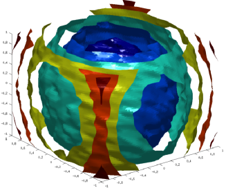
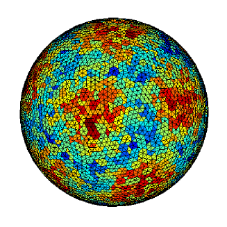
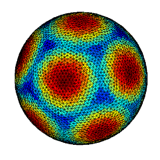
To illustrate the versatility of the method, we performed the same denoising experience in the context of support functions, using the discretization explained in Section 3. As in the previous example, we consider a support function perturbed by additive Gaussian noise $\mathrm{h}_{0}(p)=\mathrm{h}^{*}(p)+c{\mathcal{N}}(0,1)$. In the numerical application, $\mathrm{h}^{*}$ is the support function of the unit isocaedron and $c=0.05$, as shown on the left of Figure 4. Our goal is to compute the projection of $\mathrm{h}_{0}$ to the space of support functions:

$$\min_{\mathrm{h}\in\mathcal{\mathcal{H}}^{s}}\left\|\mathrm{h}-\mathrm{h}_{0}\right\|_{L^{2}(\mathcal{S}^{d-1})}^{2}.$$

In order to relax the constraint $\mathcal{H}^{s}$, we imposed one dimensional constraints on a family of $2000$ great circles of $\mathcal{S}^{d-1}$ uniformly distributed and a step discretization of every circular arc equal to $0.02$. We obtained a very satisfactory reconstruction of $\mathrm{h}_{i}$ after $10^{4}$ iterations of the SDMM algorithm, as displayed on the right of Figure 4.

Figure 4. Denoising the support function of a convex body. On the left the perturbed support function of the icosaedron. On the right its projection into the set of support functions.

6. Application II : Principal-agent problem

The principal-agent problem formalizes how a monopolist selling products can determine a set of prices for its products so as to maximize its revenue, given a distribution of customer – the agents. We describe the simplest geometric version of this problem in the next paragraph. Various instances of this problem are then used as numerical benchmarks for our relaxed convexity constraints.

6.1. Geometric principal agent problem

Let $X$ be a bounded convex domain of $\mathbb{R}^{d}$, a distribution of agent $\rho:X\to\mathbb{R}$ and a finite subset $K\subseteq X$. The monopolist or principal needs to determine a price menu $\pi$ for pick-up or deliveries, so as to maximize its revenue. The principal has to take into account the two following constraints: (i) the agents will try to maximize their utility and (ii) there is a finite subset $K\subseteq X$ of facilities, that compete with the principal and force him to set its price $\pi(y)$ to zero at any $y$ in $K$. For a given price menu $\pi$, the utility of a location $y$ for an agent located at a position $x$ in $X$ is given by $u_{\pi}(x,y)=-\frac{1}{2}\left\|x-y\right\|^{2}-\pi(y)$. The fact that each agent tries to maximize his utility means that he will choose a location that balances closeness and price. The maximum utility for an agent $x$ is given by:

$$u_{\pi}(x):=\max_{y\in X}u(x,y)=-\frac{1}{2}\left\|x\right\|^{2}+\max_{y\in X}\left[\langle x|y\rangle-\frac{1}{2}\left\|y\right\|^{2}-\pi(y)\right]$$

Let us denote $\overline{u}_{\pi}(x)$ the convex function $u_{\pi}(x)+\frac{1}{2}\left\|x\right\|^{2}$. This function is differentiable almost every point $x$ in $X$, and at such a point the gradient $\nabla\overline{u}_{\pi}(x)$ agrees with the best location for $x$, i.e. $\nabla\overline{u}_{\pi}(x)=\arg\max_{y}u(x,y)$. This implies the following equality:

$$\overline{u}_{\pi}(x)=\langle x|\nabla\overline{u}_{\pi}(x)\rangle-\frac{1}{2}\left\|\nabla\overline{u}_{\pi}(x)\right\|^{2}-\pi(\nabla\overline{u}_{\pi}(x))$$

Our final assumption is that the cost of a location for the principal is constant. Our previous discussion implies that the total revenue of the principal, given a price menu $\pi$, is computed by the following formula

$$R(\pi) =\int_{X}\pi(\nabla\overline{u}_{\pi}(x))\rho(x)\mathrm{d}x$$

$$=-\int_{X}\left[\overline{u}_{\pi}(x)-\langle x|\nabla\overline{u}_{\pi}(x)\rangle+\frac{1}{2}\left\|\nabla\overline{u}_{\pi}(x)\right\|^{2}\right]\rho(x)\mathrm{d}x$$ (6.23)

Changing the unknown from $\pi$ to $v:=\overline{u}_{\pi}$, the assumption that the price vanishes on the set $K$ translates as $u_{\pi}\geqslant\max_{y\in K}-\frac{1}{2}\left\|\cdot-y\right\|^{2}$ or equivalently

$$v(x)=\overline{u}_{\pi}(x)\geqslant\max_{y\in K}\langle x|y\rangle-\frac{1}{2}\left\|y\right\|^{2}.$$

Thus, we reformulate the principal’s problem in term of $v$ as the minimization of the following functional:

$$L(v):=\int_{X}\left[v(x)+\frac{1}{2}\left\|\nabla v(x)-x\right\|^{2}\right]\rho(x)\mathrm{d}x$$ (6.24)

where the maximum is taken over the set of convex functions $v:X\to\mathbb{R}$ that satisfy the lower bound $v\geqslant\max_{y\in K}\langle.|y\rangle-\frac{1}{2}\left\|y\right\|^{2}$.

6.2. Numerical results

We present three numerical experiments. The first one concerns a linear variant of the principal-agent problem. The second and third one concern the geometric principal-agent problem presented above: we maximize the functional $L$ of Equation (6.24) over the space of non-negative convex functions, with $X=\mathrm{B}(0,1)$ and $X=[1,2]^{2}$ respectively, $\rho$ constant and $K=\{(0,0)\}$.

# points	$\varepsilon$	$|L-L_{\mathrm{opt}}|$	$\left\|u-u_{\mathrm{opt}}\right\|_{\infty}$	CPU
$30\times 30$	$0.06$	$1.3\cdot 10^{-3}$	$2\cdot 10^{-3}$	11s
$60\times 60$	$0.03$	$9.8\cdot 10^{-4}$	$1.6\cdot 10^{-3}$	251s
$90\times 90$	$0.02$	$9.7\cdot 10^{-4}$	$1.1\cdot 10^{-3}$	500s

Table 1. Convergence of numerical approximations for the geometric principal-agent problem (radial case).

# points	$\varepsilon$	$|M-M_{\mathrm{opt}}|$	$\left\|u-u_{\mathrm{opt}}\right\|_{\infty}$	CPU
$900$	$0.06$	$8\cdot 10^{-5}$	$1.15\cdot 10^{-2}$	11s
$3600$	$0.03$	$8\cdot 10^{-5}$	$1.00\cdot 10^{-2}$	28s
$8100$	$0.02$	$4.3\cdot 10^{-5}$	$8.46\cdot 10^{-3}$	87s

Table 2. Convergence of numerical approximations for the linear principal-agent.

Linear principal agent.

As a first benchmark, we consider a variant of the principal-agent problem where the minimized functional is linear in the utility function $u$ [14]. The goal is to minimize the following functional

$$M(u):=\int_{X}(u(x)-\langle\nabla u|x\rangle)\rho(x)\mathrm{d}x,$$

where $X=[0,1]^{2}$ and $\rho=1$, over the set of convex functions whose gradient is included in $[0,1]^{2}$. The solution to this problem is known explicitely:

$$u_{\mathrm{opt}}(x_{1},x_{2})=\max\{0,x_{1}-a,x_{2}-a,x_{1}+x_{2}-b\}$$

where $a=2/3$ and $b=(4-\sqrt{2})/3$. We solve the linear principal-agent problem on a regular grid meshing $[0,1]^{2}$, and compare it to the exact solution on the grid points. Table 2 displays the numerical results for various grid sizes and choices of $\varepsilon$.

Geometric principal agent, radial case

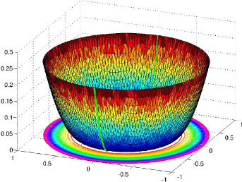
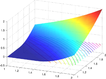
In order to evaluate the accuracy of our algorithm, we first solve the (non-linear) geometric principal-agent problem on the unit disk, with $K=\{(0,0)\}$ and $\rho$ constant. The optimal profile is radial in this setting, and one can obtain a very accurate description of the optimal radial component by solving a standard convex quadratic programming problem. In parallel, we compute an approximation of the $2$D solution on an unstructured mesh of the disk. On the left of Figure 5, we show that our solution matches the line of the one dimensional profile after $10^{3}$ iterations of the SDMM algorithm, for $\delta=0.12$ and $\varepsilon=1/50$. Table 1 shows the speed of convergence of our method, both in term of computation time and accuracy, with $10^{3}$ iterations.

Geometric principal agent, Rochet-Choné case

We recover numerically the so-called bunching phenomena predicted by Rochet and Choné [22] when $X=[1,2]^{2}$, $\rho$ is constant and $K=\{(0,0)\}$, thus confirming numerical results from [6, 17, 1]. On the right of Figure 5, we show the numerical solution defined on a regular mesh of the square of size $60\times 60$, with $\varepsilon=0.02$. In this computation, the interpolation operator is constructed using P$3$ finite elements, so as to illustrate the flexibility of our method.

Figure 5. (Left) Numerical approximation to the principal-agent problem on $X=\mathrm{B}(0,1)$, with $\delta=1/60$ and $\varepsilon=1/50$. The profile of the $1$D solution is reported as a bold line on the graph. (Right) Numerical approximation to the principal-agent problem with $X=[1,2]^{2}$ by P$3$ finite elements.

7. Application III : Closest convex set with constant width

A convex compact set $K$ of $\mathbb{R}^{d}$ has constant width $\alpha>0$ if all its projection on every straight line are segments of length $\alpha$. This property is equivalent to the following constraints on the support function of $K$ :

$$\forall\nu\in\mathcal{S}^{d-1},\,\mathrm{h}_{K}(\nu)+\mathrm{h}_{K}(-\nu)=\alpha.$$ (7.25)

Surprisingly, balls are not the only bodies having this property. In dimension two for instance, Reuleaux’s triangles, which are obtained by intersecting three disks of radius $\alpha$ centered at the vertices of an equilateral triangle have constant width $\alpha$. Moreover, Reuleaux’s triangles have been proved by Lebesgue and Blaschke to minimize the area among two-dimensional bodies with prescribed constant width.

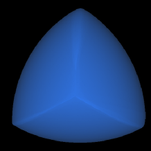
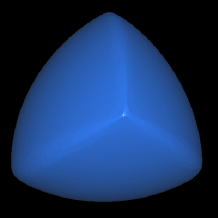
In dimension three, this problem is more difficult. Indeed the mere existence of non trivial three-dimensional bodies of constant width is not so easy to establish. In particular, no finite intersection of balls has constant width, except balls themselves [13]. As a consequence and in contrast to the two dimensional case, the intersection of four balls centered at the vertices of a regular simplex is not of constant width. In 1912, E. Meissner described in [15] a process to turn this spherical body into an asymmetric bodies with constant width, by smoothing three of its circular edges. This famous body is called “Meissner tetrahedron” in the literature [11]. It is suspected to minimize the volume among three dimensional bodies with the same constant width. Let us point out that Meissner construction is not canonical in the sense that it requires the choice the set of three edges that have to be smoothed. As a consequence, there actually exists two kinds of “Meissner tetrahedron” having the same measure.

In these two constructions, the regular simplex seems to play a crucial role in the optimality (see also [8] for a more rigorous justification of this intuition). It is therefore natural to search for the body with constant width that is the closest to a regular simplex. In an Hilbert space, the projection on a convex set is uniquely defined. Thus, the Meissner tetrahedra cannot be obtained as projections of a regular simplex to the convex set $\mathcal{H}^{s}\cap\mathcal{W}$ with respect to the $\mathrm{L}^{2}$ norm between support functions. Such an obstruction does not hold for the $\mathrm{L}^{1}$ and $\mathrm{L}^{\infty}$ norm, which are not strictly convex. We illustrate below that our relaxed approach can be used to numerically investigate these questions. The optimization problem that we have to approximate is

$$\min_{\mathrm{h}\in\mathcal{H}^{s}\cap\mathcal{W}}\left\|\mathrm{h}_{0}-\mathrm{h}\right\|_{\mathrm{L}^{p}(\mathcal{S}^{2})},~{}1\leqslant p\leqslant\infty$$

where $\mathcal{W}$ is the set of function of $\mathcal{S}^{2}$ which satisfy the width constraints (7.25).

As explained is Section 3, we relax the constraint of being a support function, by imposing convexity-like conditions on a finite family of great circles of the sphere. In the experiments presented below the number of vertices in our mesh of $\mathcal{S}^{2}$ is $5000$. We choose a family of $2000$ great circles of $\mathcal{S}^{2}$ uniformly distributed (with respect to their normal direction) and a step discretization of every circular arc equal to $0.02$. Finally, the constant width constraint $\mathcal{W}$ is approximated by imposing that antipodal values of the mesh must satisfy a set of linear equality constraints, which can be easily implemented in the proximal framework depicted in Section 4.2. Note that in this first experience, the value of the width constraint is not imposed.

Figure 6. Reconstruction of the convex bodies associated to the $\mathrm{L}^{1}$, $\mathrm{L}^{2}$ and $\mathrm{L}^{\infty}$ projection of $\mathrm{h}_{S}$ without prescribing the width value.

	Surface	Volume	Width	Relative width error
$\mathrm{L}^{1}$ projection of $\mathrm{h}_{S}$	2.6616	0.36432	0.951	< 0.001
$\mathrm{L}^{2}$ projection of $\mathrm{h}_{S}$	2.5191	0.34312	0.920	< 0.003
$\mathrm{L}^{\infty}$ projection of $\mathrm{h}_{S}$	2.1351	0.28081	0.835	< 0.001

Table 3. Numerical results for the projections of $\mathrm{h}_{S}$

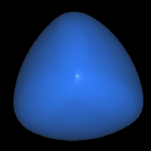
We present in Table 3 and Figure 6, our numerical description of the projections of the support function of a regular simplex in the set of support function of constant width bodies for the $\mathrm{L}^{1}$, $\mathrm{L}^{2}$ and $\mathrm{L}^{\infty}$ norms. One can observe that the resulting support functions describe a body with constant width within an error of magnitude $0.1\%$. In other words the gap between the minimal width and the diameter is relatively less than $0.001$. In the $L^{1}$ case we obtain a convex body whose surface area and volume are close to those of a Meissner body of same width, within a relative error of less than $0.01$. We also performed the same experiment starting from the support functions of others platonic solids. For any of these other solids, and when the value of the width is not imposed, the closest body with constant seems to always be a ball.

References

- [1] Néstor E Aguilera and Pedro Morin, Approximating optimization problems over convex functions, Numerische Mathematik 111 (2008), no. 1, 1–34.
- [2] Heinz H Bauschke, Regina S Burachik, Patrick L Combettes, Veit Elser, D Russell Luke, and Henry Wolkowicz, Fixed-point algorithms for inverse problems in science and engineering, (2011).
- [3] J. Bertrand, Prescription of Gauss curvature using optimal mass transport, Preprint, 2010.
- [4] Guillaume Carlier, Thomas Lachand-Robert, and Bertrand Maury, A numerical approach to variational problems subject to convexity constraint, Numerische Mathematik 88 (2001), no. 2, 299–318.
- [5] Philippe Choné and Hervé VJ Le Meur, Non-convergence result for conformal approximation of variational problems subject to a convexity constraint, Numer. Funct. Anal. Optim. 5-6 (2001), no. 22, 529–547.
- [6] Ivar Ekeland and Santiago Moreno-Bromberg, An algorithm for computing solutions of variational problems with global convexity constraints, Numerische Mathematik 115 (2010), no. 1, 45–69.
- [7] Alessio Figalli, Young-Heon Kim, and Robert J McCann, When is multidimensional screening a convex program?, Journal of Economic Theory 146 (2011), no. 2, 454–478.
- [8] HaiLin Jin and Qi Guo, Asymmetry of convex bodies of constant width, Discrete & Computational Geometry 47 (2012), no. 2, 415–423.
- [9] Richard Jordan, David Kinderlehrer, and Felix Otto, The variational formulation of the fokker–planck equation, SIAM journal on mathematical analysis 29 (1998), no. 1, 1–17.
- [10] B. Jüttler, Surface fitting using convex tensor-product splines, J. Comput. Appl. Math. 84 (1997), no. 1, 23–44.
- [11] Bernd Kawohl and Christof Weber, Meissner’s mysterious bodies, Math. Intell. 33 (2011), no. 3, 94–101.
- [12] Thomas Lachand-Robert and Édouard Oudet, Minimizing within convex bodies using a convex hull method, SIAM Journal on Optimization 16 (2005), no. 2, 368–379.
- [13] by same author, Bodies of constant width in arbitrary dimension, Mathematische Nachrichten 280 (2007), no. 7, 740–750.
- [14] Alejandro M Manelli and Daniel R Vincent, Multidimensional mechanism design: Revenue maximization and the multiple-good monopoly, Journal of Economic Theory 137 (2007), no. 1, 153–185.
- [15] E. Meissner, Über Punktmengen konstanter Breite: Drei Gipsmodelle von Flächen konstanter Breite, Zeitschrift der Mathematik und Physik 60 (1912), 92–94.
- [16] Mary C Meyer, An algorithm for quadratic programming with applications in statistics, Tech. report, Technical Report, Colorado State University, 2010.
- [17] Jean-Marie Mirebeau, Adaptive, anisotropic and hierarchical cones of discrete convex functions, arXiv preprint arXiv:1402.1561 (2014).
- [18] Adam M Oberman, A numerical method for variational problems with convexity constraints, SIAM Journal on Scientific Computing 35 (2013), no. 1, A378–A396.
- [19] V. Oliker, Embedding into with given integral Gauss curvature and optimal mass transport on , Advances in Mathematics 213 (2007), no. 2, 600–620.
- [20] Édouard Oudet, Shape optimization under width constraint, Disc. Comput. Geom. 49 (2013), no. 2, 411–428.
- [21] Hugo Raguet, Jalal Fadili, and Gabriel Peyré, A generalized forward-backward splitting, SIAM Journal on Imaging Sciences 6 (2013), no. 3, 1199–1226.
- [22] Jean-Charles Rochet and Philippe Choné, Ironing, sweeping, and multidimensional screening, Econometrica (1998), 783–826.
- [23] R. Schneider, Convex bodies: the brunn-minkowski theory, Cambridge Univ Prss, 1993.