A Mixture of Coalesced Generalized
Hyperbolic Distributions

Cristina Tortora, Brian C. Franczak∗∗, Ryan P. Browne, Paul D. McNicholas††
(Department of Mathematics & Statistics, San José State University, CA, USA.
∗∗Department of Mathematics & Statistics, MacEwan University, Edmonton, AB, Canada.
Department of Statistics and Actuarial Sciences, University of Waterloo, ON, Canada.
††Department of Mathematics and Statistics, McMaster University, ON, Canada.
)
Abstract

A mixture of multiple scaled generalized hyperbolic distributions (MMSGHDs) is introduced. Then, a coalesced generalized hyperbolic distribution (CGHD) is developed by joining a generalized hyperbolic distribution with a multiple scaled generalized hyperbolic distribution. After detailing the development of the MMSGHDs, which arises via implementation of a multi-dimensional weight function, the density of the mixture of CGHDs is developed. A parameter estimation scheme is developed using the ever-expanding class of MM algorithms and the Bayesian information criterion is used for model selection. The issue of cluster convexity is examined and a special case of the MMSGHDs is developed that is guaranteed to have convex clusters. These approaches are illustrated and compared using simulated and real data. The identifiability of the MMSGHDs and the mixture of CGHDs is discussed in an appendix.

Keywords: clustering; coalesced distributions; convexity; finite mixture models; generalized hyperbolic distribution; mixture of mixtures; MM algorithm; multiple scaled distributions.

1 Introduction

Finite mixture models have been linked with clustering since the idea of defining a cluster in terms of a component in finite mixture model was put forth more than 60 years ago (see McNicholas, 2016a, Section 2.1). Nowadays, mixture model-based clustering is a popular approach to clustering. A random vector 𝐗𝐗\mathbf{X} arises from a finite mixture model if, for all 𝐱𝐗𝐱𝐗\mathbf{x}\subset\mathbf{X}, its density can be written

f(𝐱ϑ)=g=1Gπgfg(𝐱𝜽g),𝑓conditional𝐱bold-italic-ϑsuperscriptsubscript𝑔1𝐺subscript𝜋𝑔subscript𝑓𝑔conditional𝐱subscript𝜽𝑔f(\mathbf{x}\mid\mbox{\boldmath$\vartheta$})=\sum_{g=1}^{G}\pi_{g}f_{g}(\mathbf{x}\mid\mbox{\boldmath$\theta$}_{g}),

where πg>0subscript𝜋𝑔0\pi_{g}>0 such that g=1Gπg=1superscriptsubscript𝑔1𝐺subscript𝜋𝑔1\sum_{g=1}^{G}\pi_{g}=1 are the mixing proportions, fg(𝐱𝜽g)subscript𝑓𝑔conditional𝐱subscript𝜽𝑔f_{g}(\mathbf{x}\mid\mbox{\boldmath$\theta$}_{g}) is the g𝑔gth component density, and ϑ=(𝝅,𝜽1,,𝜽G)bold-italic-ϑ𝝅subscript𝜽1subscript𝜽𝐺\mbox{\boldmath$\vartheta$}=(\mbox{\boldmath$\pi$},\mbox{\boldmath$\theta$}_{1},\ldots,\mbox{\boldmath$\theta$}_{G}) denotes the vector of parameters with 𝝅=(π1,,πG)𝝅subscript𝜋1subscript𝜋𝐺\mbox{\boldmath$\pi$}=(\pi_{1},\ldots,\pi_{G}). The component densities f1(𝐱𝜽1),,fG(𝐱𝜽G)subscript𝑓1conditional𝐱subscript𝜽1subscript𝑓𝐺conditional𝐱subscript𝜽𝐺f_{1}(\mathbf{x}\mid\mbox{\boldmath$\theta$}_{1}),\ldots,f_{G}(\mathbf{x}\mid\mbox{\boldmath$\theta$}_{G}) are typically taken to be of the same type, most commonly multivariate Gaussian. In fact, until a few years after the turn of the century, almost all work on clustering and classification using mixture models had been based on Gaussian mixture models (e.g., Banfield and Raftery, 1993; Celeux and Govaert, 1995; Ghahramani and Hinton, 1997; Tipping and Bishop, 1999; McLachlan and Peel, 2000; Fraley and Raftery, 2002).

Early work on non-Gaussian mixtures was on mixtures of multivariate t𝑡t-distributions (e.g., Peel and McLachlan, 2000). A little beyond the turn of the century, work on t𝑡t-mixtures burgeoned into a substantial subfield of mixture model-based classification (e.g., McLachlan et al., 2007; Andrews and McNicholas, 2011a, b, 2012; Baek and McLachlan, 2011; Steane et al., 2012; Lin et al., 2014; Pesevski et al., 2018). Around the same time, work on mixtures of skewed distributions took off, including work on skew-normal mixtures (e.g., Lin, 2009), skew-t𝑡t mixtures (e.g., Lin, 2010; Vrbik and McNicholas, 2012, 2014; Lee and McLachlan, 2013a, b; Murray et al., 2014), Laplace mixtures (e.g., Franczak et al., 2014), variance-gamma mixtures (McNicholas et al., 2017), generalized hyperbolic mixtures (Browne and McNicholas, 2015), and other non-elliptically contoured distributions (e.g., Karlis and Santourian, 2009; Murray et al., 2017; Tang et al., 2018). A thorough review of work on model-based clustering is given by McNicholas (2016b).

More recently, mixtures of multiple scaled distributions have been considered (Section 2). In the present manuscript, a multiple scaled generalized hyperbolic distribution is introduced (Section 3). Because the (multivariate) generalized hyperbolic distribution is not a special case of the multiple scaled generalized hyperbolic distribution, a coalesced generalized hyperbolic distribution is also developed (Section 4). The issue of cluster convexity, which has essentially been ignored in work to date on multiple scaled distributions is discussed and a special case of the multiple scaled generalized hyperbolic distribution is developed to guarantee that the components, i.e., the clusters, are convex (Section 5).

2 Multiple Scaled Distributions

The distribution of a p𝑝p-dimensional random variable 𝐗𝐗\mathbf{X} is said to be a normal variance-mean mixture if its density can be written in the form

f(𝐱𝝁,𝚺,𝜶,𝜽)=0ϕp(𝐱𝝁+w𝜶,w𝚺)h(w𝜽)𝑑w,𝑓conditional𝐱𝝁𝚺𝜶𝜽superscriptsubscript0subscriptitalic-ϕ𝑝conditional𝐱𝝁𝑤𝜶𝑤𝚺conditional𝑤𝜽differential-d𝑤f(\mathbf{x}\mid\mbox{\boldmath$\mu$},\mathbf{\Sigma},\mbox{\boldmath$\alpha$},\mbox{\boldmath$\theta$})=\int_{0}^{\infty}{\phi_{p}\left(\mathbf{x}\mid\mbox{\boldmath$\mu$}+w\mbox{\boldmath$\alpha$},w\mathbf{\Sigma}\right)h\left(w\mid\mbox{\boldmath$\theta$}\right)dw}, (1)

where ϕp(𝐱𝝁+w𝜶,w𝚺)subscriptitalic-ϕ𝑝conditional𝐱𝝁𝑤𝜶𝑤𝚺\phi_{p}\left(\mathbf{x}\mid\mbox{\boldmath$\mu$}+w\mbox{\boldmath$\alpha$},{w}\mathbf{\Sigma}\right) is the density of a p𝑝p-dimensional Gaussian distribution with mean 𝝁+w𝜶𝝁𝑤𝜶\mbox{\boldmath$\mu$}+w\mbox{\boldmath$\alpha$} and covariance matrix w𝚺𝑤𝚺w\mathbf{\Sigma}, and h(w𝜽)conditional𝑤𝜽h\left(w\mid\mbox{\boldmath$\theta$}\right) is the density of a univariate random variable W>0𝑊0W>0 that has the role of a weight function (see Barndorff-Nielsen et al., 1982; Gneiting, 1997). This weight function can take on many forms, some of which lead to density representations for well-known non-Gaussian distributions, e.g., if h(w𝜽)conditional𝑤𝜽h\left(w\mid\mbox{\boldmath$\theta$}\right) is the density of an inverse-gamma random variable with parameters (ν/2,ν/2)𝜈2𝜈2(\nu/2,\nu/2), then (1) is a representation of the skew-t𝑡t distribution with ν𝜈\nu degrees of freedom (see Demarta and McNeil, 2005; Murray et al., 2014). Further details on, and examples of, normal variance-mean mixtures are given by Barndorff-Nielsen (1978), Kotz et al. (2001), and Kotz and Nadarajah (2004), amongst others.

Now, the density of W>0𝑊0W>0 from an inverse-gamma distribution with parameters (α,β)𝛼𝛽(\alpha,\beta) is given by

h(wα,β)=wα1βαΓ(α)exp{βw},conditional𝑤𝛼𝛽superscript𝑤𝛼1superscript𝛽𝛼Γ𝛼𝛽𝑤h\left(w\mid\alpha,\beta\right)=w^{-\alpha-1}\frac{\beta^{\alpha}}{\Gamma\left(\alpha\right)}\exp\left\{-\frac{\beta}{w}\right\}, (2)

where Γ()Γ\Gamma(\cdot) is the Gamma function. Setting α=β=ν/2𝛼𝛽𝜈2\alpha=\beta=\nu/2 in (2) gives

h(wν/2,ν/2)=wν/21(ν/2)ν/2Γ(ν/2)exp{ν2w},conditional𝑤𝜈2𝜈2superscript𝑤𝜈21superscript𝜈2𝜈2Γ𝜈2𝜈2𝑤h\left(w\mid\nu/2,\nu/2\right)=w^{-\nu/2-1}\frac{(\nu/2)^{\nu/2}}{\Gamma\left(\nu/2\right)}\exp\left\{-\frac{\nu}{2w}\right\}, (3)

Setting 𝜶=𝟎𝜶0\mbox{\boldmath$\alpha$}=\mathbf{0} in (1), and using (3) for h(w𝜽)conditional𝑤𝜽h\left(w\mid\mbox{\boldmath$\theta$}\right), it follows that the density of the multivariate t𝑡t-distribution with ν𝜈\nu degrees of freedom can be written

ft(𝐱𝝁,𝚺,ν)subscript𝑓𝑡conditional𝐱𝝁𝚺𝜈\displaystyle f_{t}(\mathbf{x}\mid\mbox{\boldmath$\mu$},\mathbf{\Sigma},\nu) =0ϕp(𝐱𝝁,w𝚺)h(wν/2,ν/2)𝑑wabsentsuperscriptsubscript0subscriptitalic-ϕ𝑝conditional𝐱𝝁𝑤𝚺conditional𝑤𝜈2𝜈2differential-d𝑤\displaystyle=\int_{0}^{\infty}{\phi_{p}\left(\mathbf{x}\mid\mbox{\boldmath$\mu$},w\mathbf{\Sigma}\right)h\left(w\mid\nu/2,\nu/2\right)dw}
=Γ([ν+p]/2)|𝚺|1/2(πν)p/2Γ(ν/2)[1+δ(𝐱,𝝁|𝚺)/ν](ν+p)/2absentΓdelimited-[]𝜈𝑝2superscript𝚺12superscript𝜋𝜈𝑝2Γ𝜈2superscriptdelimited-[]1𝛿𝐱conditional𝝁𝚺𝜈𝜈𝑝2\displaystyle=\frac{\Gamma\left([{\nu+p}]/{2}\right)|\mathbf{\Sigma}|^{-{1}/{2}}}{(\pi\nu)^{{p}/{2}}\Gamma\left({\nu}/{2}\right)\left[1+{\delta(\mathbf{x},\mbox{\boldmath$\mu$}~{}|~{}\mathbf{\Sigma})}/{\nu}\right]^{{(\nu+p)}/{2}}} (4)

where δ(𝐱,𝝁𝚺)𝛿𝐱conditional𝝁𝚺\delta\left(\mathbf{x},\mbox{\boldmath$\mu$}\mid\mathbf{\Sigma}\right) is the squared Mahalanobis distance between 𝐱𝐱\mathbf{x} and 𝝁𝝁\mu. Forbes and Wraith (2014) show that a multi-dimensional weight variable

𝚫𝐖=diag(w11,,wp1)subscript𝚫𝐖diagsuperscriptsubscript𝑤11superscriptsubscript𝑤𝑝1\mathbf{\Delta}_{\mathbf{W}}=\,\mbox{diag}\left(w_{1}^{-1},\dots,w_{p}^{-1}\right)

can be incorporated into (1) via an eigen-decomposition of the symmetric positive-definite matrix 𝚺𝚺\mathbf{\Sigma}. Specifically, they set 𝚺=𝚪𝚽𝚪,𝚺𝚪𝚽superscript𝚪\mathbf{\Sigma}=\mathbf{\Gamma}\mathbf{\Phi}\mathbf{\Gamma}^{\prime}, where 𝚪𝚪\mathbf{\Gamma} is a p×p𝑝𝑝p\times p matrix of eigenvectors and 𝚽𝚽\mathbf{\Phi} is a p×p𝑝𝑝p\times p diagonal matrix containing the eigenvalues of 𝚺𝚺\mathbf{\Sigma}. It follows that the density of 𝐗𝐗\mathbf{X} becomes

f(𝐱𝝁,𝚪,𝚽,𝜶,𝜽)=00ϕp(𝐱𝝁+𝚫𝐖𝜶,𝚪𝚫𝐖𝚽𝚪)h𝐖(w1,,wp𝜽)𝑑w1𝑑wp,𝑓conditional𝐱𝝁𝚪𝚽𝜶𝜽superscriptsubscript0superscriptsubscript0subscriptitalic-ϕ𝑝conditional𝐱𝝁subscript𝚫𝐖𝜶𝚪subscript𝚫𝐖𝚽superscript𝚪subscript𝐖subscript𝑤1conditionalsubscript𝑤𝑝𝜽differential-dsubscript𝑤1differential-dsubscript𝑤𝑝\begin{split}f&\left(\mathbf{x}\mid\mbox{\boldmath$\mu$},\mathbf{\Gamma},\mathbf{\Phi},\mbox{\boldmath$\alpha$},\mbox{\boldmath$\theta$}\right)=\\ &\int_{0}^{\infty}\cdots\int_{0}^{\infty}\phi_{p}\left(\mathbf{x}\mid\mbox{\boldmath$\mu$}+\mathbf{\Delta}_{\mathbf{W}}\mbox{\boldmath$\alpha$},\mathbf{\Gamma}\mathbf{\Delta}_{\mathbf{W}}\mathbf{\Phi}\mathbf{\Gamma}^{\prime}\right)h_{\mathbf{W}}\left(w_{1},\dots,w_{p}\mid\mbox{\boldmath$\theta$}\right)dw_{1}\dots dw_{p},\end{split} (5)

where

h𝐖(w1,,wp𝜽)=h(w1𝜽1)××h(wp𝜽p)subscript𝐖subscript𝑤1conditionalsubscript𝑤𝑝𝜽conditionalsubscript𝑤1subscript𝜽1conditionalsubscript𝑤𝑝subscript𝜽𝑝h_{\mathbf{W}}\left(w_{1},\dots,w_{p}\mid\mbox{\boldmath$\theta$}\right)=h\left(w_{1}\mid\mbox{\boldmath$\theta$}_{1}\right)\times\dots\times h\left(w_{p}\mid\mbox{\boldmath$\theta$}_{p}\right)

is a p𝑝p-dimensional density such that the random variables W1,,Wpsubscript𝑊1subscript𝑊𝑝W_{1},\ldots,W_{p} are independent, i.e., the weights are independent. The density given in (5) adds flexibility to normal variance-mean mixtures because the parameters 𝜽1,,𝜽psubscript𝜽1subscript𝜽𝑝\mbox{\boldmath$\theta$}_{1},\dots,\mbox{\boldmath$\theta$}_{p} are free to vary in each dimension. Using the density in (5), Forbes and Wraith (2014) derive the density of a multiple scaled multivariate-t𝑡t distribution, Wraith and Forbes (2015) derive a multiple scaled normal-inverse Gaussian distribution, and Franczak et al. (2015) develop a multiple scaled shifted asymmetric Laplace distribution.

Setting 𝚺=𝚪𝚽𝚪𝚺𝚪𝚽superscript𝚪\mathbf{\Sigma}=\mathbf{\Gamma}\mathbf{\Phi}\mathbf{\Gamma}^{\prime}, it follows from (5) that the density of a multiple scaled analogue of (2) can be written

ftMS(𝐱𝝁,𝚪,𝚽,𝝂)=00ϕp(𝐱𝝁,𝚪𝚽𝚫𝐖𝚪)h𝐖(w1,,wp𝝂)𝑑w1𝑑wp,subscript𝑓𝑡MSconditional𝐱𝝁𝚪𝚽𝝂superscriptsubscript0superscriptsubscript0subscriptitalic-ϕ𝑝conditional𝐱𝝁𝚪𝚽subscript𝚫𝐖superscript𝚪subscript𝐖subscript𝑤1conditionalsubscript𝑤𝑝𝝂differential-dsubscript𝑤1differential-dsubscript𝑤𝑝\begin{split}&f_{t\text{\tiny{MS}}}(\mathbf{x}\mid\mbox{\boldmath$\mu$},\mathbf{\Gamma},\mathbf{\Phi},\mbox{\boldmath$\nu$})=\int_{0}^{\infty}\cdots\int_{0}^{\infty}\phi_{p}\left(\mathbf{x}\mid\mbox{\boldmath$\mu$},\mathbf{\Gamma}\mathbf{\Phi}\mathbf{\Delta}_{\mathbf{W}}\mathbf{\Gamma}^{\prime}\right)h_{\mathbf{W}}\left(w_{1},\dots,w_{p}\mid\mbox{\boldmath$\nu$}\right)dw_{1}\dots dw_{p},\end{split} (6)

where 𝚫𝐖=diag(w11,,wp1)subscript𝚫𝐖diagsuperscriptsubscript𝑤11superscriptsubscript𝑤𝑝1\mathbf{\Delta}_{\mathbf{W}}=\,\mbox{diag}\left(w_{1}^{-1},\dots,w_{p}^{-1}\right) and the weight function

h𝐖(w1,,wp𝝂)=h(w1ν1/2,ν1/2)××h(wpνp/2,νp/2)subscript𝐖subscript𝑤1conditionalsubscript𝑤𝑝𝝂conditionalsubscript𝑤1subscript𝜈12subscript𝜈12conditionalsubscript𝑤𝑝subscript𝜈𝑝2subscript𝜈𝑝2h_{\mathbf{W}}\left(w_{1},\dots,w_{p}\mid\mbox{\boldmath$\nu$}\right)=h\left(w_{1}\mid\nu_{1}/2,\nu_{1}/2\right)\times\dots\times h\left(w_{p}\mid\nu_{p}/2,\nu_{p}/2\right)

is a p𝑝p-dimensional Gamma density, where h(wjνj/2,νj/2)conditionalsubscript𝑤𝑗subscript𝜈𝑗2subscript𝜈𝑗2h\left(w_{j}\mid\nu_{j}/2,\nu_{j}/2\right) is given by (3). Note that the scaled Gaussian density in (LABEL:eq:nvmm_dens2) can be written

ϕp(𝐱𝝁,𝚪𝚽𝚫𝐖𝚪)subscriptitalic-ϕ𝑝conditional𝐱𝝁𝚪𝚽subscript𝚫𝐖superscript𝚪\displaystyle\phi_{p}\left(\mathbf{x}\mid\mbox{\boldmath$\mu$},\mathbf{\Gamma}\mathbf{\Phi}\mathbf{\Delta}_{\mathbf{W}}\mathbf{\Gamma}^{\prime}\right) =j=1pϕ1([𝚪𝐱]j[𝚪𝝁]j,Φjwj1)=j=1pϕ1([𝚪(𝐱𝝁)]j0,Φjwj1),absentsuperscriptsubscriptproduct𝑗1𝑝subscriptitalic-ϕ1conditionalsubscriptdelimited-[]superscript𝚪𝐱𝑗subscriptdelimited-[]superscript𝚪𝝁𝑗subscriptΦ𝑗superscriptsubscript𝑤𝑗1superscriptsubscriptproduct𝑗1𝑝subscriptitalic-ϕ1conditionalsubscriptdelimited-[]superscript𝚪𝐱𝝁𝑗0subscriptΦ𝑗superscriptsubscript𝑤𝑗1\displaystyle=\prod_{j=1}^{p}{\phi_{1}\left([\mathbf{\Gamma}^{\prime}\mathbf{x}]_{j}\mid[\mathbf{\Gamma}^{\prime}\mbox{\boldmath$\mu$}]_{j},\Phi_{j}w_{j}^{-1}\right)}=\prod_{j=1}^{p}{\phi_{1}\left([\mathbf{\Gamma}^{\prime}(\mathbf{x}-\mbox{\boldmath$\mu$})]_{j}\mid 0,\Phi_{j}w_{j}^{-1}\right)}, (7)

where ϕ1([𝚪(𝐱𝝁)]j0,Φjwj1)subscriptitalic-ϕ1conditionalsubscriptdelimited-[]superscript𝚪𝐱𝝁𝑗0subscriptΦ𝑗superscriptsubscript𝑤𝑗1\phi_{1}\left([\mathbf{\Gamma}^{\prime}(\mathbf{x}-\mbox{\boldmath$\mu$})]_{j}\mid 0,\Phi_{j}w_{j}^{-1}\right) is the density of a univariate Gaussian distribution with mean 00 and variance Φjwj1subscriptΦ𝑗superscriptsubscript𝑤𝑗1\Phi_{j}w_{j}^{-1}, [𝚪(𝐱𝝁)]jsubscriptdelimited-[]superscript𝚪𝐱𝝁𝑗[\mathbf{\Gamma}^{\prime}(\mathbf{x}-\mbox{\boldmath$\mu$})]_{j} is the j𝑗jth element of 𝚪(𝐱𝝁)superscript𝚪𝐱𝝁\mathbf{\Gamma}^{\prime}(\mathbf{x}-\mbox{\boldmath$\mu$}), and ΦjsubscriptΦ𝑗\Phi_{j} is the j𝑗jth eigenvalue of 𝚽𝚽\mathbf{\Phi}, i.e., the j𝑗jth diagonal element of the matrix 𝚽𝚽\mathbf{\Phi}. It follows that (LABEL:eq:nvmm_dens2) can be written

ftMS(𝐱𝝁,𝚪,𝚽,𝝂)=j=1p0ϕ1([𝚪(𝐱𝝁)]j0,Φjwj1)h(wjνj/2,νj/2)dwj.subscript𝑓𝑡MS𝐱𝝁𝚪𝚽𝝂superscriptsubscriptproduct𝑗1𝑝superscriptsubscript0subscriptitalic-ϕ1subscriptdelimited-[]superscript𝚪𝐱𝝁𝑗0subscriptΦ𝑗superscriptsubscript𝑤𝑗1subscript𝑤𝑗subscript𝜈𝑗2subscript𝜈𝑗2𝑑subscript𝑤𝑗\begin{split}f_{t\text{\tiny{MS}}}(\mathbf{x}\mid\mbox{\boldmath$\mu$},&\mathbf{\Gamma},\mathbf{\Phi},\mbox{\boldmath$\nu$})=\prod_{j=1}^{p}\int_{0}^{\infty}{\phi_{1}\left([\mathbf{\Gamma}^{\prime}(\mathbf{x}-\mbox{\boldmath$\mu$})]_{j}\mid 0,\Phi_{j}w_{j}^{-1}\right)h\left(w_{j}\mid\nu_{j}/2,\nu_{j}/2\right)dw_{j}}.\end{split} (8)

Solving the integral in (8) gives the density of a multiple scaled multivariate-t𝑡t distribution,

ftMS(𝐱𝝁,𝚪,𝚽,𝝂)=j=1pΓ([νj+1]/2)Γ(νj/2)(Φjνjπ)1/2[1+[𝚪(𝐱𝝁)]j2Φjνj](νj+1)/2,subscript𝑓𝑡MSconditional𝐱𝝁𝚪𝚽𝝂superscriptsubscriptproduct𝑗1𝑝Γdelimited-[]subscript𝜈𝑗12Γsubscript𝜈𝑗2superscriptsubscriptΦ𝑗subscript𝜈𝑗𝜋12superscriptdelimited-[]1superscriptsubscriptdelimited-[]superscript𝚪𝐱𝝁𝑗2subscriptΦ𝑗subscript𝜈𝑗subscript𝜈𝑗12f_{t\text{\tiny{MS}}}(\mathbf{x}\mid\mbox{\boldmath$\mu$},\mathbf{\Gamma},\mathbf{\Phi},\mbox{\boldmath$\nu$})=\prod_{j=1}^{p}{\frac{\Gamma([\nu_{j}+1]/2)}{\Gamma(\nu_{j}/2)(\Phi_{j}\nu_{j}\pi)^{1/2}}\left[1+\frac{[\mathbf{\Gamma}^{\prime}(\mathbf{x}-\mbox{\boldmath$\mu$})]_{j}^{2}}{\Phi_{j}\nu_{j}}\right]^{-(\nu_{j}+1)/2}}, (9)

where ΦjsubscriptΦ𝑗\Phi_{j} is the j𝑗jth eigenvalue of 𝚽𝚽\mathbf{\Phi}, 𝚪𝚪\mathbf{\Gamma} is a matrix of eigenvectors, 𝝁𝝁\mu is a location parameter, and [𝚪(𝐱𝝁)]j2/Φjsuperscriptsubscriptdelimited-[]superscript𝚪𝐱𝝁𝑗2subscriptΦ𝑗[\mathbf{\Gamma}^{\prime}(\mathbf{x}-\mbox{\boldmath$\mu$})]_{j}^{2}/\Phi_{j} can be regarded as the squared Mahalanobis distance between 𝐱𝐱\mathbf{x} and 𝝁𝝁\mu.

The main difference between the traditional multivariate-t𝑡t density given in (2) and the multiple scaled multivariate-t𝑡t density given in (9) is that the degrees of freedom can now be parameterized separately in each dimension j𝑗j. Therefore, unlike the standard multivariate-t𝑡t distribution, the multiple scaled density in (9) can account for different tail weight in each dimension (Forbes and Wraith, 2014).

3 Mixture of Multiple Scaled Generalized Hyperbolic Distributions

There are different ways to formulate the density of a generalized hyperbolic distribution (GHD; see McNeil et al., 2005, for example). Browne and McNicholas (2015) use a mixture of GHDs (MGHDs) for clustering and they use the following formulation for the density of a p𝑝p-dimensional random vector 𝐗𝐗\mathbf{X} from a GHD:

fGH(𝐱𝜽)=[ω+δ(𝐱,𝝁|𝚺)ω+𝜶𝚺1𝜶](λp/2)/2Kλp/2([ω+𝜶𝚺1𝜶][ω+δ(𝐱,𝝁|𝚺)])(2π)p/2|𝚺|1/2Kλ(ω)exp{(𝐱𝝁)𝚺1𝜶},subscript𝑓GHconditional𝐱𝜽superscriptdelimited-[]𝜔𝛿𝐱conditional𝝁𝚺𝜔superscript𝜶superscript𝚺1𝜶𝜆𝑝22subscript𝐾𝜆𝑝2delimited-[]𝜔superscript𝜶superscript𝚺1𝜶delimited-[]𝜔𝛿𝐱conditional𝝁𝚺superscript2𝜋𝑝2superscript𝚺12subscript𝐾𝜆𝜔superscript𝐱𝝁superscript𝚺1𝜶\begin{split}f_{\text{GH}}(\mathbf{x}\mid\mbox{\boldmath$\theta$})=&\left[\frac{\omega+\delta\left(\mathbf{x},\mbox{\boldmath$\mu$}|\mathbf{\Sigma}\right)}{\omega+\mbox{\boldmath$\alpha$}^{\prime}\mathbf{\Sigma}^{-1}\mbox{\boldmath$\alpha$}}\right]^{(\lambda-{p}/{2})/2}\frac{K_{\lambda-{p}/{2}}\Big{(}\sqrt{\big{[}\omega+\mbox{\boldmath$\alpha$}^{\prime}\mathbf{\Sigma}^{-1}\mbox{\boldmath$\alpha$}\big{]}\big{[}\omega+\delta\left(\mathbf{x},\mbox{\boldmath$\mu$}|\mathbf{\Sigma}\right)\big{]}}\Big{)}}{\left(2\pi\right)^{{p}/{2}}\left|\mathbf{\Sigma}\right|^{{1}/{2}}K_{\lambda}\left(\omega\right)\exp\big{\{}-\left(\mathbf{x}-\mbox{\boldmath$\mu$}\right)^{\prime}\mathbf{\Sigma}^{-1}\mbox{\boldmath$\alpha$}\big{\}}},\end{split} (10)

where 𝝁p𝝁superscript𝑝\mbox{\boldmath$\mu$}\in\mathbb{R}^{p} is the location parameter, 𝜶p𝜶superscript𝑝\mbox{\boldmath$\alpha$}\in\mathbb{R}^{p} is the skewness parameter, 𝚺p×p𝚺superscript𝑝𝑝\mathbf{\Sigma}\in\mathbb{R}^{p\times p} is the scale matrix, λ𝜆\lambda\in\mathbb{R} is the index parameter, ω+𝜔superscript\omega\in\mathbb{R}^{+} is the concentration parameter, and Kλsubscript𝐾𝜆K_{\lambda} is the modified Bessel function of the third kind with index λ𝜆\lambda. Now, 𝐗wN(𝝁+w𝜶,w𝚺)conditional𝐗𝑤N𝝁𝑤𝜶𝑤𝚺\mathbf{X}\mid w\backsim\text{N}(\mbox{\boldmath$\mu$}+w\mbox{\boldmath$\alpha$},w\mathbf{\Sigma}) and W𝐱GIG(ω+𝜶𝚺1𝜶,ω+δ(𝐱,𝝁|𝚺),λp/2),similar-toconditional𝑊𝐱GIG𝜔superscript𝜶superscript𝚺1𝜶𝜔𝛿𝐱conditional𝝁𝚺𝜆𝑝2W\mid\mathbf{x}\sim\text{GIG}(\omega+\mbox{\boldmath$\alpha$}^{\prime}\mathbf{\Sigma}^{-1}\mbox{\boldmath$\alpha$},\omega+\delta\left(\mathbf{x},\mbox{\boldmath$\mu$}|\mathbf{\Sigma}\right),\lambda-{p}/{2}), where WGIG(a,b,λ)similar-to𝑊GIG𝑎𝑏𝜆W\sim\text{GIG}(a,b,\lambda) denotes that W𝑊W follows a generalized inverse Gaussian (GIG) distribution with density formulated as

q(w|a,b,λ)=(a/b)λ/2wλ12Kλ(ab)exp{aw+b/w2},𝑞conditional𝑤𝑎𝑏𝜆superscript𝑎𝑏𝜆2superscript𝑤𝜆12subscript𝐾𝜆𝑎𝑏𝑎𝑤𝑏𝑤2q(w~{}|~{}a,b,\lambda)=\frac{(a/b)^{\lambda/2}w^{\lambda-1}}{2K_{\lambda}(\sqrt{ab})}\exp\left\{-\frac{aw+b/w}{2}\right\}, (11)

for w>0𝑤0w>0, where a,b+𝑎𝑏superscripta,b\in\mathbb{R}^{+}, and λ𝜆\lambda\in\mathbb{R}. The GIG distribution has some attractive properties including the tractability of the following expected values:

𝔼[W]=baKλ+1(ab)Kλ(ab),𝔼[1/W]=abKλ+1(ab)Kλ(ab)2λb,formulae-sequence𝔼delimited-[]𝑊𝑏𝑎subscript𝐾𝜆1𝑎𝑏subscript𝐾𝜆𝑎𝑏𝔼delimited-[]1𝑊𝑎𝑏subscript𝐾𝜆1𝑎𝑏subscript𝐾𝜆𝑎𝑏2𝜆𝑏\displaystyle\mathbb{E}\left[W\right]=\sqrt{\frac{b}{a}}\frac{K_{\lambda+1}\big{(}\sqrt{ab}\big{)}}{K_{\lambda}(\sqrt{ab})},\qquad\qquad\mathbb{E}\left[{1}/{W}\right]=\sqrt{\frac{a}{b}}\frac{K_{\lambda+1}\big{(}\sqrt{ab}\big{)}}{K_{\lambda}\big{(}\sqrt{ab}\big{)}}-\frac{2\lambda}{b}, (12)
𝔼[logW]=log(ba)+1Kλ(ab)λKλ(ab).𝔼delimited-[]𝑊𝑏𝑎1subscript𝐾𝜆𝑎𝑏𝜆subscript𝐾𝜆𝑎𝑏\displaystyle\mathbb{E}[\log W]=\log\left(\sqrt{\frac{b}{a}}\right)+\frac{1}{K_{\lambda}\big{(}\sqrt{ab}\big{)}}\frac{\partial}{\partial\lambda}K_{\lambda}\big{(}\sqrt{ab}\big{)}. (13)

Write 𝐗GHD(𝝁,𝚺,𝜶,ω,λ)similar-to𝐗GHD𝝁𝚺𝜶𝜔𝜆\mathbf{X}\sim\text{GHD}(\mbox{\boldmath$\mu$},\mathbf{\Sigma},\mbox{\boldmath$\alpha$},\omega,\lambda) to denote that the p𝑝p-dimensional random variable 𝐗𝐗\mathbf{X} has the density in (10).

Now, note that the formulation of the GHD in (10) can be written as a normal variance-mean mixture where the univariate density is GIG, i.e.,

𝐗=𝝁+W𝜶+W𝐕,𝐗𝝁𝑊𝜶𝑊𝐕\mathbf{X}=\mbox{\boldmath$\mu$}+W\mbox{\boldmath$\alpha$}+\sqrt{W}\mathbf{V}, (14)

where 𝐕N(𝟎,𝚺)similar-to𝐕N0𝚺\mathbf{V}\sim\text{N}(\mathbf{0},\mathbf{\Sigma}) and W𝑊W has density

h(wω,1,λ)=wλ12Kλ(ω)exp{ω2(w+1w)},conditional𝑤𝜔1𝜆superscript𝑤𝜆12subscript𝐾𝜆𝜔𝜔2𝑤1𝑤h(w\mid\omega,1,\lambda)=\frac{w^{\lambda-1}}{2K_{\lambda}(\omega)}\exp{\left\{-\frac{\omega}{2}\left(w+\frac{1}{w}\right)\right\}}, (15)

for w>0𝑤0w>0, where ω𝜔\omega and λ𝜆\lambda are as previously defined. Note that (15) is just an alternative parameterization of the GIG distribution. From (14) and (15), it follows that the generalized hyperbolic density can be written

f(𝐱𝝁,𝚺,𝜶,ω,λ)=0ϕp(𝐱𝝁+w𝜶,w𝚺)h(wω,1,λ)𝑑w.𝑓conditional𝐱𝝁𝚺𝜶𝜔𝜆superscriptsubscript0subscriptitalic-ϕ𝑝conditional𝐱𝝁𝑤𝜶𝑤𝚺conditional𝑤𝜔1𝜆differential-d𝑤f(\mathbf{x}\mid\mbox{\boldmath$\mu$},\mathbf{\Sigma},\mbox{\boldmath$\alpha$},\omega,\lambda)=\int_{0}^{\infty}{\phi_{p}\left(\mathbf{x}\mid\mbox{\boldmath$\mu$}+w\mbox{\boldmath$\alpha$},{w}\mathbf{\Sigma}\right)h(w\mid\omega,1,\lambda)dw}. (16)

We can use (5), (16) and an alternative parameterization to write the density of a multiple scaled generalized hyperbolic distribution (MSGHD) as

fMSGHD(𝐱𝝁,𝚪,𝚽,𝜶,𝝎,𝝀)=00ϕp(𝚪𝐱𝝁𝚫𝐰𝜶𝟎,𝚫𝐰𝚽)h𝐰(w1,,wp𝝎,𝟏,𝝀)𝑑w1𝑑wp,subscript𝑓MSGHD𝐱𝝁𝚪𝚽𝜶𝝎𝝀superscriptsubscript0superscriptsubscript0subscriptitalic-ϕ𝑝superscript𝚪𝐱𝝁conditionalsubscript𝚫𝐰𝜶0subscript𝚫𝐰𝚽subscript𝐰subscript𝑤1conditionalsubscript𝑤𝑝𝝎1𝝀differential-dsubscript𝑤1differential-dsubscript𝑤𝑝\begin{split}f_{\text{\tiny{MSGHD}}}(&\mathbf{x}\mid\mbox{\boldmath$\mu$},\mathbf{\Gamma},\mathbf{\Phi},\mbox{\boldmath$\alpha$},\mbox{\boldmath$\omega$},\mbox{\boldmath$\lambda$})=\\ &\int_{0}^{\infty}\dots\int_{0}^{\infty}\phi_{p}\left(\mathbf{\Gamma}^{\prime}\mathbf{x}-\mbox{\boldmath$\mu$}-\mathbf{\Delta}_{\mathbf{w}}\mbox{\boldmath$\alpha$}\mid\mathbf{0},\mathbf{\Delta}_{\mathbf{w}}\mathbf{\Phi}\right)h_{\mathbf{w}}(w_{1},\dots,w_{p}\mid\mbox{\boldmath$\omega$},\mathbf{1},\mbox{\boldmath$\lambda$})dw_{1}\dots dw_{p},\end{split} (17)

where 𝝎=(ω1,,ωp)𝝎superscriptsubscript𝜔1subscript𝜔𝑝\mbox{\boldmath$\omega$}=(\omega_{1},\ldots,\omega_{p})^{\prime}, 𝝀=(λ1,,λp)𝝀superscriptsubscript𝜆1subscript𝜆𝑝\mbox{\boldmath$\lambda$}=(\lambda_{1},\ldots,\lambda_{p})^{\prime}, 𝟏1\mathbf{1} is a p𝑝p-vector of 111s, and

h𝐖(w1,,wp𝝎,𝟏,𝝀)=h(w1ω1,1,λ1)××h(wpωp,1,λp).subscript𝐖subscript𝑤1conditionalsubscript𝑤𝑝𝝎1𝝀conditionalsubscript𝑤1subscript𝜔11subscript𝜆1conditionalsubscript𝑤𝑝subscript𝜔𝑝1subscript𝜆𝑝h_{\mathbf{W}}(w_{1},\dots,w_{p}\mid\mbox{\boldmath$\omega$},\mathbf{1},\mbox{\boldmath$\lambda$})=h(w_{1}\mid\omega_{1},1,\lambda_{1})\times\dots\times h(w_{p}\mid\omega_{p},1,\lambda_{p}).

From (LABEL:eq:nvmm_dens2) and (7), it follows that (17) can be written

fMSGHD(𝐱𝝁,𝚪,𝚽,𝜶,𝝎,𝝀)=j=1p0ϕ1([𝚪𝐱𝝁𝚫𝐰𝜶]j0,Φjwj)hW(wjωj,1,λj)𝑑wjsubscript𝑓MSGHDconditional𝐱𝝁𝚪𝚽𝜶𝝎𝝀superscriptsubscriptproduct𝑗1𝑝superscriptsubscript0subscriptitalic-ϕ1conditionalsubscriptdelimited-[]superscript𝚪𝐱𝝁subscript𝚫𝐰𝜶𝑗0subscriptΦ𝑗subscript𝑤𝑗subscript𝑊conditionalsubscript𝑤𝑗subscript𝜔𝑗1subscript𝜆𝑗differential-dsubscript𝑤𝑗\displaystyle f_{\text{\tiny{MSGHD}}}\left(\mathbf{x}\mid\mbox{\boldmath$\mu$},\mathbf{\Gamma},\mathbf{\Phi},\mbox{\boldmath$\alpha$},\mbox{\boldmath$\omega$},\mbox{\boldmath$\lambda$}\right)=\prod_{j=1}^{p}\int_{0}^{\infty}{\phi_{1}\big{(}\left[\mathbf{\Gamma}^{\prime}\mathbf{x}-\mbox{\boldmath$\mu$}-\mathbf{\Delta}_{\mathbf{w}}\mbox{\boldmath$\alpha$}\right]_{j}\mid 0,\Phi_{j}w_{j}\big{)}h_{W}\left(w_{j}\mid\omega_{j},1,\lambda_{j}\right)dw_{j}}
=j=1p{[ωj+Φj1([𝚪𝐱]jμj)2ωj+αj2Φj1]λj1/22Kλj1/2([ωj+αj2Φj1][ωj+Φj1([𝚪𝐱]jμj)2])(2π)1/2Φj1/2Kλj(ωj)exp{([𝚪𝐱]jμj)Φj1αj}},absentsuperscriptsubscriptproduct𝑗1𝑝superscriptdelimited-[]subscript𝜔𝑗superscriptsubscriptΦ𝑗1superscriptsubscriptdelimited-[]superscript𝚪𝐱𝑗subscript𝜇𝑗2subscript𝜔𝑗superscriptsubscript𝛼𝑗2superscriptsubscriptΦ𝑗1subscript𝜆𝑗122subscript𝐾subscript𝜆𝑗12delimited-[]subscript𝜔𝑗superscriptsubscript𝛼𝑗2superscriptsubscriptΦ𝑗1delimited-[]subscript𝜔𝑗superscriptsubscriptΦ𝑗1superscriptsubscriptdelimited-[]superscript𝚪𝐱𝑗subscript𝜇𝑗2superscript2𝜋12superscriptsubscriptΦ𝑗12subscript𝐾subscript𝜆𝑗subscript𝜔𝑗subscriptdelimited-[]superscript𝚪𝐱𝑗subscript𝜇𝑗superscriptsubscriptΦ𝑗1subscript𝛼𝑗\displaystyle=\prod_{j=1}^{p}\left\{\left[\frac{\omega_{j}+\Phi_{j}^{-1}\big{(}\left[\mathbf{\Gamma}^{\prime}\mathbf{x}\right]_{j}-\mu_{j}\big{)}^{2}}{\omega_{j}+\alpha_{j}^{2}{\Phi_{j}}^{-1}}\right]^{\frac{\lambda_{j}-{1}/{2}}{2}}\frac{K_{\lambda_{j}-{1}/{2}}\bigg{(}\sqrt{\left[\omega_{j}+\alpha_{j}^{2}{\Phi_{j}}^{-1}\right]\left[\omega_{j}+\Phi_{j}^{-1}\big{(}\left[\mathbf{\Gamma}^{\prime}\mathbf{x}\right]_{j}-\mu_{j}\big{)}^{2}\right]}\bigg{)}}{(2\pi)^{{1}/{2}}{\Phi_{j}}^{{1}/{2}}K_{\lambda_{j}}(\omega_{j})\exp{\left\{-\big{(}\left[\mathbf{\Gamma}^{\prime}\mathbf{x}\right]_{j}-\mu_{j}\big{)}{\Phi_{j}^{-1}\alpha_{j}}\right\}}}\right\},

where [𝚪𝐱]jsubscriptdelimited-[]superscript𝚪𝐱𝑗\left[\mathbf{\Gamma}^{\prime}\mathbf{x}\right]_{j} is the j𝑗jth element of the vector 𝚪𝐱superscript𝚪𝐱\mathbf{\Gamma}^{\prime}\mathbf{x}, μjsubscript𝜇𝑗\mu_{j} is the j𝑗jth element of the location parameter 𝝁𝝁\mu, αjsubscript𝛼𝑗\alpha_{j} is the j𝑗jth element of the skewness parameter 𝜶𝜶\alpha, 𝚪𝚪\mathbf{\Gamma} is a p×p𝑝𝑝p\times p matrix of eigenvectors, ΦjsubscriptΦ𝑗\Phi_{j} is the j𝑗jth eigenvalue of the diagonal matrix 𝚽𝚽\mathbf{\Phi}, 𝝎=(ω1,,ωp)𝝎superscriptsubscript𝜔1subscript𝜔𝑝\mbox{\boldmath$\omega$}=(\omega_{1},\ldots,\omega_{p})^{\prime} controls the concentration in each dimension p𝑝p, and 𝝀=(λ1,,λp)𝝀superscriptsubscript𝜆1subscript𝜆𝑝\mbox{\boldmath$\lambda$}=(\lambda_{1},\ldots,\lambda_{p})^{\prime} is a p𝑝p-dimensional index parameter. Write 𝐗MSGHD(𝝁,𝚪,𝚽,𝜶,𝝎,𝝀)𝐗MSGHD𝝁𝚪𝚽𝜶𝝎𝝀\mathbf{X}\backsim\text{MSGHD}(\mbox{\boldmath$\mu$},\mathbf{\Gamma},\mathbf{\Phi},\mbox{\boldmath$\alpha$},\mbox{\boldmath$\omega$},\mbox{\boldmath$\lambda$}) to indicate that the random vector 𝐗𝐗\mathbf{X} follows an MSGHD with density fMSGHD(𝐱𝝁,𝚪,𝚽,𝜶,𝝎,𝝀)subscript𝑓MSGHDconditional𝐱𝝁𝚪𝚽𝜶𝝎𝝀f_{\text{\tiny{MSGHD}}}(\mathbf{x}\mid\mbox{\boldmath$\mu$},\mathbf{\Gamma},\mathbf{\Phi},\mbox{\boldmath$\alpha$},\mbox{\boldmath$\omega$},\mbox{\boldmath$\lambda$}). Then, a mixture of MSGHDs (MMSGHDs) has density

f(𝐱ϑ)=g=1GπgfMSGHD(𝐱𝝁g,𝚪g,𝚽g,𝜶g,𝝎g,𝝀g).𝑓conditional𝐱bold-italic-ϑsuperscriptsubscript𝑔1𝐺subscript𝜋𝑔subscript𝑓MSGHDconditional𝐱subscript𝝁𝑔subscript𝚪𝑔subscript𝚽𝑔subscript𝜶𝑔subscript𝝎𝑔subscript𝝀𝑔f(\mathbf{x}\mid\mbox{\boldmath$\vartheta$})=\sum_{g=1}^{G}\pi_{g}f_{\text{\tiny{MSGHD}}}\left(\mathbf{x}\mid\mbox{\boldmath$\mu$}_{g},\mathbf{\Gamma}_{g},\mathbf{\Phi}_{g},\mbox{\boldmath$\alpha$}_{g},\mbox{\boldmath$\omega$}_{g},\mbox{\boldmath$\lambda$}_{g}\right). (18)

The identifiability of the MMSGHD is discussed in Appendix C.

4 Mixture of Coalesced Generalized Hyperbolic Distributions

Note that the generalized hyperbolic distribution is not a special or limiting case of the MSGHD under any parameterization with p>1𝑝1p>1. Motivated by this, consider a coalesced generalized hyperbolic distribution (CGHD) that contains both the generalized hyperbolic distribution and MSGHD as limiting cases. The CGHD arises through the introduction of a random vector

𝐑=U𝐗+(1U)𝐒,𝐑𝑈𝐗1𝑈𝐒\mathbf{R}=U\mathbf{X}+(1-U)\mathbf{S}, (19)

where 𝐗=𝚪𝐘𝐗𝚪𝐘\mathbf{X}=\mathbf{\Gamma}\mathbf{Y}, 𝐘GHD(𝝁,𝚺,𝜶,ω0,λ0)𝐘GHD𝝁𝚺𝜶subscript𝜔0subscript𝜆0\mathbf{Y}\backsim\text{GHD}\left(\mbox{\boldmath$\mu$},\mathbf{\Sigma},\mbox{\boldmath$\alpha$},\omega_{0},\lambda_{0}\right), 𝚺=𝚪𝚽𝚪𝚺𝚪𝚽superscript𝚪\mathbf{\Sigma}=\mathbf{\Gamma}\mathbf{\Phi}\mathbf{\Gamma}^{\prime}, 𝐒MSGHD(𝝁,𝚪,𝚽,𝜶,𝝎,𝝀)𝐒MSGHD𝝁𝚪𝚽𝜶𝝎𝝀\mathbf{S}\backsim\text{MSGHD}\left(\mbox{\boldmath$\mu$},\mathbf{\Gamma},\mathbf{\Phi},\mbox{\boldmath$\alpha$},\mbox{\boldmath$\omega$},\mbox{\boldmath$\lambda$}\right), and U𝑈U is an indicator variable such that

U={1 if 𝐑 follows a generalized hyperbolic distribution, and0 if 𝐑 follows a MSGHD.𝑈cases1 if 𝐑 follows a generalized hyperbolic distribution, and0 if 𝐑 follows a MSGHD.U=\begin{cases}1&\text{ if }\mathbf{R}\text{ follows a generalized hyperbolic distribution, and}\\ 0&\text{ if }\mathbf{R}\text{ follows a MSGHD.}\end{cases}

It follows that 𝐗=𝚪𝝁+W𝚪𝜶+W𝚪𝐕,𝐗𝚪𝝁𝑊𝚪𝜶𝑊𝚪𝐕\mathbf{X}=\mathbf{\Gamma}\mbox{\boldmath$\mu$}+W\mathbf{\Gamma}\mbox{\boldmath$\alpha$}+\sqrt{W}\mathbf{\Gamma}\mathbf{V}, where 𝚪𝐕Np(𝟎,𝚪𝚽𝚪)𝚪𝐕subscriptN𝑝0𝚪𝚽superscript𝚪\mathbf{\Gamma}\mathbf{V}\backsim\text{N}_{p}\left(\mathbf{0},\mathbf{\Gamma}\mathbf{\Phi}\mathbf{\Gamma}^{\prime}\right), 𝐒=𝚪𝝁+𝚪𝜶𝚫𝐰+𝚪𝐀,𝐒𝚪𝝁𝚪𝜶subscript𝚫𝐰𝚪𝐀\mathbf{S}=\mathbf{\Gamma}\mbox{\boldmath$\mu$}+\mathbf{\Gamma}\mbox{\boldmath$\alpha$}\mathbf{\Delta}_{\mathbf{w}}+\mathbf{\Gamma}\mathbf{A}, where 𝚪𝐀Np(𝟎,𝚪𝚫𝐰𝚽𝚪)𝚪𝐀subscriptN𝑝0𝚪subscript𝚫𝐰𝚽superscript𝚪\mathbf{\Gamma}\mathbf{A}\backsim\text{N}_{p}\left(\mathbf{0},\mathbf{\Gamma}\mathbf{\Delta}_{\mathbf{w}}\mathbf{\Phi}\mathbf{\Gamma}^{\prime}\right), and the density of 𝐑𝐑\mathbf{R} can be written

fCGHD(𝐫𝝁,𝚪,𝚽,𝜶,𝝎,𝝀,ω0,λ0,ϖ)=ϖfGHD(𝐫𝝁,𝚪𝚽𝚪,𝜶,ω0,λ0)+(1ϖ)fMSGHD(𝐫𝝁,𝚪,𝚽,𝜶,𝝎,𝝀),subscript𝑓CGHD𝐫𝝁𝚪𝚽𝜶𝝎𝝀subscript𝜔0subscript𝜆0italic-ϖitalic-ϖsubscript𝑓GHDconditional𝐫𝝁𝚪𝚽superscript𝚪𝜶subscript𝜔0subscript𝜆01italic-ϖsubscript𝑓MSGHDconditional𝐫𝝁𝚪𝚽𝜶𝝎𝝀\begin{split}f_{\text{\tiny{CGHD}}}(\mathbf{r}\mid\mbox{\boldmath$\mu$},&\mathbf{\Gamma},\mathbf{\Phi},\mbox{\boldmath$\alpha$},\mbox{\boldmath$\omega$},\mbox{\boldmath$\lambda$},\omega_{0},\lambda_{0},\varpi)\\ &=\varpi f_{\text{\tiny{GHD}}}\left(\mathbf{r}\mid\mbox{\boldmath$\mu$},\mathbf{\Gamma}\mathbf{\Phi}\mathbf{\Gamma}^{\prime},\mbox{\boldmath$\alpha$},\omega_{0},\lambda_{0}\right)+(1-\varpi)f_{\text{\tiny{MSGHD}}}\left(\mathbf{r}\mid\mbox{\boldmath$\mu$},\mathbf{\Gamma},\mathbf{\Phi},\mbox{\boldmath$\alpha$},\mbox{\boldmath$\omega$},\mbox{\boldmath$\lambda$}\right),\end{split} (20)

where fGHD()subscript𝑓GHDf_{\text{\tiny{GHD}}}(\cdot) is the density of a generalized hyperbolic random variable, fMSGHD()subscript𝑓MSGHDf_{\text{\tiny{MSGHD}}}(\cdot) is the density of a MSGHD random variable, and ϖ(0,1)italic-ϖ01\varpi\in(0,1) is a mixing proportion. Note that the random vector 𝐑𝐑\mathbf{R} would be distributed generalized hyperbolic if ϖ=1italic-ϖ1\varpi=1 and would be distributed MSGHD if ϖ=0italic-ϖ0\varpi=0. However, we must restrict ϖ(0,1)italic-ϖ01\varpi\in(0,1) for identifiability reasons. Specifically, if ϖ=0italic-ϖ0\varpi=0 then the value of fCGHD(𝐫𝝁,𝚪,𝚽,𝜶,𝝎,𝝀,ω0,λ0,ϖ)subscript𝑓CGHDconditional𝐫𝝁𝚪𝚽𝜶𝝎𝝀subscript𝜔0subscript𝜆0italic-ϖf_{\text{\tiny{CGHD}}}(\mathbf{r}\mid\mbox{\boldmath$\mu$},\mathbf{\Gamma},\mathbf{\Phi},\mbox{\boldmath$\alpha$},\mbox{\boldmath$\omega$},\mbox{\boldmath$\lambda$},\omega_{0},\lambda_{0},\varpi) will be the same for any ω0subscript𝜔0\omega_{0} and λ0subscript𝜆0\lambda_{0} whereas, if ϖ=1italic-ϖ1\varpi=1, then the value of fCGHD(𝐫𝝁,𝚪,𝚽,𝜶,𝝎,𝝀,ω0,λ0,ϖ)subscript𝑓CGHDconditional𝐫𝝁𝚪𝚽𝜶𝝎𝝀subscript𝜔0subscript𝜆0italic-ϖf_{\text{\tiny{CGHD}}}(\mathbf{r}\mid\mbox{\boldmath$\mu$},\mathbf{\Gamma},\mathbf{\Phi},\mbox{\boldmath$\alpha$},\mbox{\boldmath$\omega$},\mbox{\boldmath$\lambda$},\omega_{0},\lambda_{0},\varpi) will be the same for any 𝝎𝝎\omega and 𝝀𝝀\lambda. The parameters 𝝁𝝁\mu, 𝜶𝜶\alpha, 𝚪𝚪\mathbf{\Gamma}, and 𝚽𝚽\mathbf{\Phi} are the same for both densities, the parameters ω0subscript𝜔0\omega_{0} and λ0subscript𝜆0\lambda_{0} are univariate values peculiar to the generalized hyperbolic distribution, and the p𝑝p-dimensional parameters 𝝎𝝎\omega and 𝝀𝝀\lambda are peculiar to the MSGHD. Write 𝐑CGHD(𝝁,𝚪,𝚽,𝜶,𝝎,𝝀,ω0,λ0,ϖ)𝐑CGHD𝝁𝚪𝚽𝜶𝝎𝝀subscript𝜔0subscript𝜆0italic-ϖ\mathbf{R}\backsim\text{CGHD}(\mbox{\boldmath$\mu$},\mathbf{\Gamma},\mathbf{\Phi},\mbox{\boldmath$\alpha$},\mbox{\boldmath$\omega$},\mbox{\boldmath$\lambda$},\omega_{0},\lambda_{0},\varpi) to indicate that the random vector 𝐑𝐑\mathbf{R} follows a CGHD with density in (20).

A mixture of CGHDs (MCGHDs) has density

f(𝐱ϑ)=g=1GπgfCGHD(𝐱𝝁g,𝚪g,𝚽g,𝜶g,𝝎g,𝝀g,ω0g,λ0g,ϖg).𝑓conditional𝐱bold-italic-ϑsuperscriptsubscript𝑔1𝐺subscript𝜋𝑔subscript𝑓CGHDconditional𝐱subscript𝝁𝑔subscript𝚪𝑔subscript𝚽𝑔subscript𝜶𝑔subscript𝝎𝑔subscript𝝀𝑔subscript𝜔0𝑔subscript𝜆0𝑔subscriptitalic-ϖ𝑔f(\mathbf{x}\mid\mbox{\boldmath$\vartheta$})=\sum_{g=1}^{G}\pi_{g}f_{\text{\tiny{CGHD}}}\left(\mathbf{x}\mid\mbox{\boldmath$\mu$}_{g},\mathbf{\Gamma}_{g},\mathbf{\Phi}_{g},\mbox{\boldmath$\alpha$}_{g},\mbox{\boldmath$\omega$}_{g},\mbox{\boldmath$\lambda$}_{g},\omega_{0g},\lambda_{0g},\varpi_{g}\right).

Parameter estimation can be carried out via a generalized expectation-maximization (GEM) algorithm (Dempster et al., 1977). There are four sources of missing data: the latent w0igsubscript𝑤0𝑖𝑔w_{0ig}, the multi-dimensional weights 𝚫𝐰ig=diag(w1ig,,wpig)subscript𝚫𝐰𝑖𝑔diagsubscript𝑤1𝑖𝑔subscript𝑤𝑝𝑖𝑔\mathbf{\Delta}_{\mathbf{w}ig}=\,\mbox{diag}(w_{1ig},\ldots,w_{pig}), the component membership labels zigsubscript𝑧𝑖𝑔z_{ig}, and the inner component labels uigsubscript𝑢𝑖𝑔u_{ig}, for i=1,,n𝑖1𝑛i=1,\ldots,n and g=1,,G𝑔1𝐺g=1,\ldots,G. As usual, zig=1subscript𝑧𝑖𝑔1z_{ig}=1 if observation i𝑖i belongs to component g𝑔g and zig=0subscript𝑧𝑖𝑔0z_{ig}=0 otherwise. Similarly, uig=1subscript𝑢𝑖𝑔1u_{ig}=1 if observation i𝑖i, in component g𝑔g, is distributed generalized hyperbolic and uig=0subscript𝑢𝑖𝑔0u_{ig}=0 if observation i𝑖i, in component g𝑔g, is distributed MSGHD. It follows that the complete-data log-likelihood for the MCGHD is

lc=i=1ng=1G{ziglogπg+ziguiglogϖg+zig(1uig)log(1ϖg)+ziguiglogh(w0ig|ω0g,1,λ0g)+zig(1uig)j=1plogh(wjig|ωjg,1,λjg)+ziguiglogϕp(𝚪g𝐱i|𝝁g+w0ig𝜶g,w0ig𝚽)+zig(1uig)j=1plogϕ1([𝚪g𝐱i]j|μjg+wjigαjg,ωjgϕjg)}.subscript𝑙csuperscriptsubscript𝑖1𝑛superscriptsubscript𝑔1𝐺subscript𝑧𝑖𝑔subscript𝜋𝑔subscript𝑧𝑖𝑔subscript𝑢𝑖𝑔subscriptitalic-ϖ𝑔subscript𝑧𝑖𝑔1subscript𝑢𝑖𝑔1subscriptitalic-ϖ𝑔subscript𝑧𝑖𝑔subscript𝑢𝑖𝑔|subscript𝑤0𝑖𝑔subscript𝜔0𝑔1subscript𝜆0𝑔subscript𝑧𝑖𝑔1subscript𝑢𝑖𝑔superscriptsubscript𝑗1𝑝conditionalsubscript𝑤𝑗𝑖𝑔subscript𝜔𝑗𝑔1subscript𝜆𝑗𝑔subscript𝑧𝑖𝑔subscript𝑢𝑖𝑔subscriptitalic-ϕ𝑝conditionalsuperscriptsubscript𝚪𝑔subscript𝐱𝑖subscript𝝁𝑔subscript𝑤0𝑖𝑔subscript𝜶𝑔subscript𝑤0𝑖𝑔𝚽subscript𝑧𝑖𝑔1subscript𝑢𝑖𝑔superscriptsubscript𝑗1𝑝subscriptitalic-ϕ1|subscriptdelimited-[]superscriptsubscript𝚪𝑔subscript𝐱𝑖𝑗subscript𝜇𝑗𝑔subscript𝑤𝑗𝑖𝑔subscript𝛼𝑗𝑔subscript𝜔𝑗𝑔subscriptitalic-ϕ𝑗𝑔\begin{split}l_{\text{c}}&=\sum_{i=1}^{n}\sum_{g=1}^{G}\bigg{\{}z_{ig}\log\pi_{g}+z_{ig}{u_{ig}}\log\varpi_{g}+z_{ig}(1-u_{ig})\log(1-\varpi_{g})+z_{ig}{u_{ig}}\log h\left(w_{0ig}~{}|~{}\omega_{0g},1,\lambda_{0g}\right)\\ &+z_{ig}(1-u_{ig})\sum_{j=1}^{p}\log h\left(w_{jig}~{}|~{}\omega_{jg},1,\lambda_{jg}\right)+z_{ig}{u_{ig}}\log\phi_{p}\left(\mathbf{\Gamma}_{g}^{\prime}\mathbf{x}_{i}~{}|~{}\mbox{\boldmath$\mu$}_{g}+w_{0ig}\mbox{\boldmath$\alpha$}_{g},w_{0ig}\mathbf{\Phi}\right)\\ &+z_{ig}(1-u_{ig})\sum_{j=1}^{p}\log\phi_{1}\left([\mathbf{\Gamma}_{g}^{\prime}\mathbf{x}_{i}]_{j}~{}|~{}\mu_{jg}+w_{jig}\alpha_{jg},\omega_{jg}\phi_{jg}\right)\bigg{\}}.\end{split}

Further details on parameter estimation (Appendix A) and the identifiability of the MCGHD (Appendix C) are discussed in appendices.

5 Cluster Convexity

The definition of clusters has been discussed quite extensively in the literature. Recently, Hennig (2015) provides a very interesting discussion of some potential characteristics that clusters may have. Even though they cannot always be observed — and, in some situations, desired characteristics may even conflict — such characteristics provide important links and contrasts between different definitions that are used for a cluster. In fact, the idea of desirable characteristics is not a new one, e.g., Cormack (1971) gives internal cohesion and external isolation as two “basic ideas” in this direction. In this paper, we follow the definition given by McNicholas (2016a): “a cluster is a unimodal component within an appropriate finite mixture model”. The term appropriate means that the model has the flexibility to fit the data and, in many cases, this also means that each cluster is convex (see McNicholas, 2016a, Section 9.1). The development of flexible models outlined herein may make it a little easier to find an “appropriate” component density.

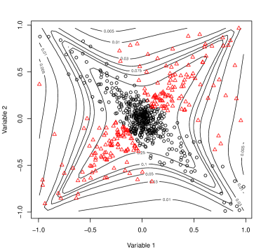
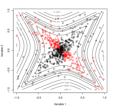
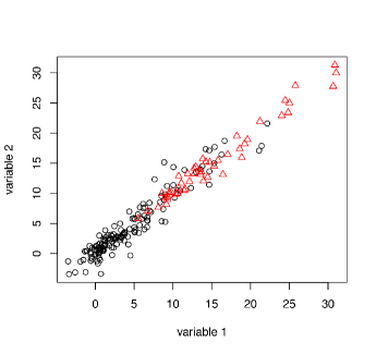
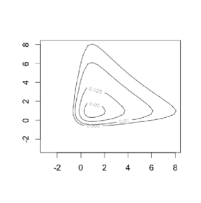
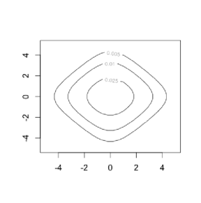
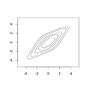
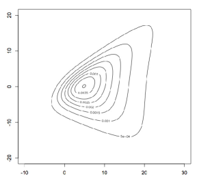
The MSGHD is more flexible than the GHD; however, similar to the multiple scaled multivariate t𝑡t-distribution of Forbes and Wraith (2014), the MSGHD can have contours that are not convex. Accordingly, the MMSGHD can have components that are non-convex, leading to non-convex clusters. Consider the data in Figure 1. How many clusters are there? The most plausible answer to this question is two overlapping clusters: one with positive correlation between the variables and another with negative correlation between the variables. There may also be an argument for four or five. Note that the data are generated from a G=2𝐺2G=2 component mixture of multivariate t𝑡t-distributions.

Refer to caption
Refer to caption
Refer to caption
Refer to caption
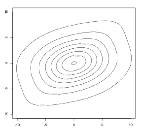
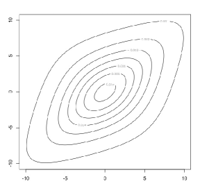
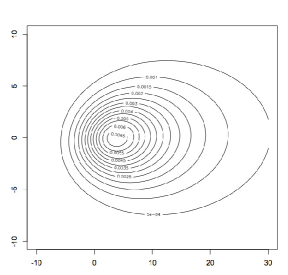
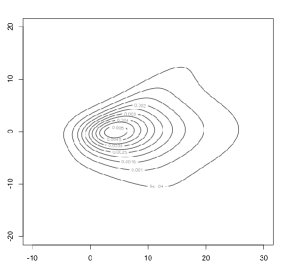
Figure 1: Scatter plot of data generated from a two-component t𝑡t-mixture (top-left) along with contours from fitted G=1𝐺1G=1 component MMSGHD (top-right), G=2𝐺2G=2 component MMSGHD (bottom-left), and G=2𝐺2G=2 component McMSGHD (bottom-right) models, where plotting symbol and colour represent predicted classifications.

The MMSGHD is fitted to these data for G=1,,5𝐺15G=1,\ldots,5 and, as is common in model-based clustering applications, the Bayesian information criterion (BIC; Schwarz, 1978) is used to select G𝐺G. Note that the BIC is given by

BIC=2l(^ϑ)ρlogn,BIC2𝑙^absentbold-italic-ϑ𝜌𝑛\text{BIC}=2l(\hat{}\mbox{\boldmath$\vartheta$})-\rho\log n,

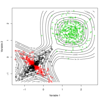
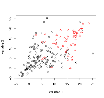
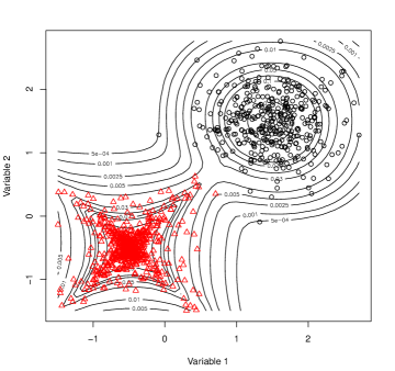
where l(^ϑ)𝑙^absentbold-italic-ϑl(\hat{}\mbox{\boldmath$\vartheta$}) is the maximized log-likelihood, ρ𝜌\rho is the number of free parameters, and n𝑛n is the number of observations. For the MMSGHD, the BIC selects a G=1𝐺1G=1 component model (Figure 1). Furthermore, looking at the G=2𝐺2G=2 component MSGHD solution (Figure 1) confirms that the problem is not just one of model selection; the G=2𝐺2G=2 component MSGHD solution selects one component that is roughy elliptical and another that is not convex. On the other hand, forcing the MSGHD to be convex — which can be done by imposing the constraint λj>1subscript𝜆𝑗1\lambda_{j}>1, for j=1,,p𝑗1𝑝j=1,\ldots,p — leads to what we call the convex MSGHD (cMSGHD). Fitting the corresponding mixture of cMSGHDs (McMSGHDs) ensures that, if each component is associated with a cluster, then convex clusters are guaranteed. Results in a G=2𝐺2G=2 component model being selected (Figure 1). Formally, this amounts to insuring that the MSGHD is quasi-convex; see Appendix B. The general point here is that if convexity is not enforced, then the MSGHD can give components that contain multiple clusters. While it is easy to spot this in two dimensions, e.g., Figure 1, this phenomenon may go unrecognized in higher dimensions, possibly resulting in greatly misleading results. Of course, the issue of non-convex clusters does not arise with most model-based approaches; however, when multiple scaled mixtures are considered, the issue can crop up. Another example in a similar vein is given in Figure 2, where data are generated from a G=3𝐺3G=3 component mixture of multivariate t𝑡t-distributions. The selected MMSGHD has G=2𝐺2G=2 components, including one clearly non-convex cluster, while the McMSGHD gives sensible clustering results.

Refer to caption
Refer to caption
Refer to caption
Figure 2: Scatter plots for model-based clustering results on data simulated from a three-component t𝑡t-mixture (top-left), with contours from the selected MMSGHD (top-right) and McMSGHD (bottom) models, respectively, where plotting symbol and colour represent predicted classifications.

The intention behind the introduction of the McMSGHD is not that it should supplant the MMSGHD, but rather that it provides a convenient check on the number of components. In a higher dimensional application, where visualization is difficult or impossible, situations where the selected MMSGHD has fewer components than the selected McMSGHD will deserve special attention. Of course, this is not to say that the selected McMSGHD will always have more components in situations where the MSGHD has too few, but rather that it will help to avoid the sort of situations depicted in Figures 1 and 2. Note that parameter estimation for the McMSGHD is analogous to the algorithm for the MMSGHD algorithm but λkjsubscript𝜆𝑘𝑗\lambda_{kj} (k=0,1,,G𝑘01𝐺k=0,1,\ldots,G, j=1,,p𝑗1𝑝j=1,\ldots,p) is updated only if the value of its update exceeds 1.

6 Illustrations

6.1 Implementation and Evaluation

In the following illustrations, we fit the MGHDs, the MMSGHDs, the McMSGHDs, and the MCGHDs using the corresponding functions available in the MixGHD package (Tortora et al., 2017) for R (R Core Team, 2017). We use k𝑘k-means and k𝑘k-medoids clustering to initialize the z^igsubscript^𝑧𝑖𝑔\hat{z}_{ig}. The adjusted Rand index (ARI; Hubert and Arabie, 1985) is used to compare predicted classifications with true classes. The ARI corrects the Rand index (Rand, 1971) for chance, its expected value under random classification is 00, and it takes a value of 111 when there is perfect class agreement. Steinley (2004) gives guidelines for interpreting ARI values.

Several mixtures of skewed distributions have been proposed for model-based clustering and classification. Among them, three different formulations of the multivariate skew-t distribution have been used for clustering in the mixture setting. The formulation used by Murray et al. (2014) is a special case of the generalized hyperbolic distributions. Azzalini et al. (2016) refers to the other two formulations as the classical and SDB formulations (for the initials of the authors’ names), respectively. Lee and McLachlan (2013b, 2014) compare the mixture of classical skew-t distributions to the mixture of SDB skew-t distributions (MSDBST) and to skew-normal analogues of both formulations; their results lead one to believe that the MSDBST is generally preferable (see Azzalini et al., 2016, for an alternative viewpoint). The MSDBST approach is implemented using the EMMIXuskew package (Lee and McLachlan, 2013a) for R and it is used for comparison herein.

6.2 Simulation Study

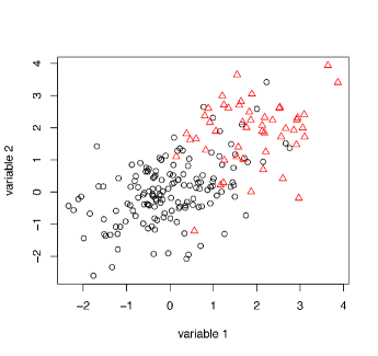
We use a simulation study to measure the performance of the proposed methods. The interest is to observe the ARI under different circumstances, the data are generated using two-component mixtures of Gaussian (Scenario 1), generalized hyperbolic (Scenario 2), and multiple scaled generalized hyperbolic distributions (Scenario 3), using the R function mvrnorm and the stochastic relationships given in (14) and Section 4. For each scenario a three factors full factorial design was used, where the factors are: medium (M) or high (H) correlation, 25% or 50% overlapping, and same (S), n1=n2=100subscript𝑛1subscript𝑛2100n_{1}=n_{2}=100, or different (D), n1=150subscript𝑛1150n_{1}=150 and n2=50subscript𝑛250n_{2}=50, number of elements per component. In all the scenarios 𝝁1=𝟏subscript𝝁11\mbox{\boldmath$\mu$}_{1}=\bf 1. Table 1 shows the average ARI, with standard deviation, obtained on 10 data sets generated from a Gaussian distribution with p=10𝑝10p=10, G=2𝐺2G=2, correlation equal to 0.33 for M and 0.66 for H, 𝝁2=𝟐subscript𝝁22\mbox{\boldmath$\mu$}_{2}=\bf 2 for 25% overlapping and 𝝁2=𝟑subscript𝝁23\mbox{\boldmath$\mu$}_{2}=\bf 3 for 50% overlapping. Table 2 shows the average ARI, with standard deviation, obtained on 10 data sets generated from a MGHD distribution with p=10𝑝10p=10, G=2𝐺2G=2, 𝜶=𝟏𝜶1\mbox{\boldmath$\alpha$}=\bf 1, λ=0.5𝜆0.5\lambda=0.5, ω=1𝜔1\omega=1 and correlation equal to 0.25 for M and 0.5 for H, 𝝁2=𝟏𝟎subscript𝝁210\mbox{\boldmath$\mu$}_{2}=\bf 10 for 25% overlapping and 𝝁2=𝟏𝟓subscript𝝁215\mbox{\boldmath$\mu$}_{2}=\bf 15 for 50% overlapping. Table 3 shows the average ARI, with 1 standard deviation, obtained on 10 data sets generated from a MMSGHD distribution with p=10𝑝10p=10, G=2𝐺2G=2, 𝜶1=𝟏subscript𝜶11\mbox{\boldmath$\alpha$}_{1}=\bf 1, 𝜶2=𝟏subscript𝜶21\mbox{\boldmath$\alpha$}_{2}=\bf-1, 𝝀=0.5𝝀0.5\mbox{\boldmath$\lambda$}=\bf 0.5, 𝝎=𝟏𝝎1\mbox{\boldmath$\omega$}=\bf 1 and correlation equal to 0.25 for M and 0.35 for H, 𝝁2=𝟏𝟗subscript𝝁219\mbox{\boldmath$\mu$}_{2}=\bf 19 for 25% overlapping and 𝝁2=𝟐𝟑subscript𝝁223\mbox{\boldmath$\mu$}_{2}=\bf 23 for 50% overlapping. For the data sets generated using the MGHD and the MMSGHD the values of the correlation had to be reduced in order to maintain 25% and 50% overlap, higher correlation lead to higher overlap. Figure 3 shows the scatterplots of the data simulated using the two-component MGDs, MGHDs, and MMSGHDs with high correlation, 50% overlapping and cluster of different size, where plotting symbol and colour represent the true classifications.

Table 1: Average ARI values, with standard deviations, for each data set generated from MGDs, with different starting parameters.
Correlation Overlapping ngsubscript𝑛𝑔n_{g} MCGHD MGHD MMSGHD McMSGHD
M 25% S 0.9640.9640.964 (0.020)0.020(0.020) 0.9320.9320.932 (0.056)0.056(0.056) 0.9430.9430.943 (0.025)0.025(0.025) 0.9410.9410.941 (0.026)0.026(0.026)
H 25% S 0.8500.8500.850 (0.044)0.044(0.044) 0.7300.7300.730 (0.132)0.132(0.132) 0.8480.8480.848 (0.050)0.050(0.050) 0.8170.8170.817 (0.062)0.062(0.062)
M 50% S 0.7340.7340.734 (0.064)0.064(0.064) 0.6420.6420.642 (0.085)0.085(0.085) 0.7360.7360.736 (0.062)0.062(0.062) 0.7210.7210.721 (0.084)0.084(0.084)
H 50% S 0.5650.5650.565 (0.116)0.116(0.116) 0.4080.4080.408 (0.179)0.179(0.179) 0.5950.5950.595 (0.059)0.059(0.059) 0.5530.5530.553 (0.090)0.090(0.090)
M 25% D 0.9810.9810.981 (0.016)0.016(0.016) 0.9790.9790.979 (0.017)0.017(0.017) 0.9810.9810.981 (0.021)0.021(0.021) 0.9750.9750.975 (0.022)0.022(0.022)
H 25% D 0.8310.8310.831 (0.047)0.047(0.047) 0.7710.7710.771 (0.047)0.047(0.047) 0.7800.7800.780 (0.082)0.082(0.082) 0.7870.7870.787 (0.059)0.059(0.059)
M 50% D 0.7150.7150.715 (0.053)0.053(0.053) 0.6630.6630.663 (0.064)0.064(0.064) 0.7050.7050.705 (0.069)0.069(0.069) 0.6960.6960.696 (0.073)0.073(0.073)
H 50% D 0.4940.4940.494 (0.133)0.133(0.133) 0.3540.3540.354 (0.151)0.151(0.151) 0.4460.4460.446 (0.122)0.122(0.122) 0.4470.4470.447 (0.130)0.130(0.130)
Table 2: Average ARI values, with standard deviations, for each data set generated from MGHDs, with different starting parameters and 𝜶=𝟏𝜶1\mbox{\boldmath$\alpha$}=\bf 1.
Correlation Overlapping ngsubscript𝑛𝑔n_{g} MCGHD MGHD MMSGHD McMSGHD
M 25% S 0.9330.9330.933 (0.045)0.045(0.045) 0.9220.9220.922 (0.041)0.041(0.041) 0.7650.7650.765 (0.228)0.228(0.228) 0.7730.7730.773 (0.211)0.211(0.211)
H 25% S 0.8420.8420.842 (0.040)0.040(0.040) 0.7700.7700.770 (0.119)0.119(0.119) 0.4630.4630.463 (0.348)0.348(0.348) 0.3990.3990.399 (0.371)0.371(0.371)
M 50% S 0.7120.7120.712 (0.093)0.093(0.093) 0.6800.6800.680 (0.107)0.107(0.107) 0.5100.5100.510 (0.229)0.229(0.229) 0.4770.4770.477 (0.221)0.221(0.221)
H 50% S 0.4750.4750.475 (0.176)0.176(0.176) 0.4160.4160.416 (0.104)0.104(0.104) 0.1880.1880.188 (0.180)0.180(0.180) 0.1590.1590.159 (0.113)0.113(0.113)
M 25% D 0.8360.8360.836 (0.058)0.058(0.058) 0.8580.8580.858 (0.058)0.058(0.058) 0.5790.5790.579 (0.233)0.233(0.233) 0.5570.5570.557 (0.233)0.233(0.233)
H 25% D 0.7540.7540.754 (0.106)0.106(0.106) 0.7130.7130.713 (0.124)0.124(0.124) 0.2570.2570.257 (0.250)0.250(0.250) 0.3180.3180.318 (0.283)0.283(0.283)
M 50% D 0.6300.6300.630 (0.092)0.092(0.092) 0.6220.6220.622 (0.098)0.098(0.098) 0.1440.1440.144 (0.134)0.134(0.134) 0.1940.1940.194 (0.198)0.198(0.198)
H 50% D 0.4270.4270.427 (0.090)0.090(0.090) 0.3600.3600.360 (0.086)0.086(0.086) 0.1210.1210.121 (0.109)0.109(0.109) 0.1270.1270.127 (0.093)0.093(0.093)
Table 3: Average ARI, with standard deviations, for each data set generated from MMSGHDs, with different starting parameters and 𝜶=𝟏𝜶1\mbox{\boldmath$\alpha$}=\bf 1.
Correlation Overlapping ngsubscript𝑛𝑔n_{g} MCGHD MGHD MMSGHD McMSGHD
M 25% S 0.9030.9030.903 (0.047)0.047(0.047) 0.8010.8010.801 (0.077)0.077(0.077) 0.9120.9120.912 (0.043)0.043(0.043) 0.9220.9220.922 (0.045)0.045(0.045)
H 25% S 0.8060.8060.806 (0.085)0.085(0.085) 0.6970.6970.697 (0.069)0.069(0.069) 0.7930.7930.793 (0.073)0.073(0.073) 0.8100.8100.810 (0.060)0.060(0.060)
M 50% S 0.7510.7510.751 (0.080)0.080(0.080) 0.6140.6140.614 (0.081)0.081(0.081) 0.8110.8110.811 (0.053)0.053(0.053) 0.8220.8220.822 (0.044)0.044(0.044)
H 50% S 0.5920.5920.592 (0.062)0.062(0.062) 0.4750.4750.475 (0.121)0.121(0.121) 0.6030.6030.603 (0.090)0.090(0.090) 0.6340.6340.634 (0.078)0.078(0.078)
M 25% D 0.9250.9250.925 (0.042)0.042(0.042) 0.8380.8380.838 (0.108)0.108(0.108) 0.9500.9500.950 (0.042)0.042(0.042) 0.9500.9500.950 (0.037)0.037(0.037)
H 25% D 0.8130.8130.813 (0.049)0.049(0.049) 0.7400.7400.740 (0.088)0.088(0.088) 0.8240.8240.824 (0.066)0.066(0.066) 0.8150.8150.815 (0.070)0.070(0.070)
M 50% D 0.7860.7860.786 (0.090)0.090(0.090) 0.6160.6160.616 (0.104)0.104(0.104) 0.7420.7420.742 (0.126)0.126(0.126) 0.7460.7460.746 (0.120)0.120(0.120)
H 50% D 0.6050.6050.605 (0.111)0.111(0.111) 0.5110.5110.511 (0.118)0.118(0.118) 0.3910.3910.391 (0.231)0.231(0.231) 0.4020.4020.402 (0.224)0.224(0.224)
Refer to caption
Refer to caption
Refer to caption
Figure 3: Scatter plots for data simulated from a two-component MGDs (top-left), MGHDs (top-right) and MMSGHDs (bottom) models, respectively, with high correlation, 50% overlapping and clusters of different size, where plotting symbol and colour represent the true classifications.

The MCGHDs perform at least comparably to the best of the MMSGHDs and MGHDs. As expected, the MGHDs over performs the MMSGHDs when the data are generated using a MGHDs model and vice versa when the data are generated from a MMSGHDs. The two methods perform similarly on normally distributed clusters. The generated clusters are all convex and that explains the similarity of the results obtained using MMSGHDs and McMSGHDs. The level of overlapping has a notable impact on the ARI, as expected. The performance of all the methods are slightly better when the clusters are of the same size and when there is a lower correlation.

6.3 Real Data Analysis

To assess the classification performance of the MGHDs, the MMSGHDs, the McMSGHDs, the MCGHDs, and the MSDBST, we consider four real data sets that are commonly used within the model-based clustering literature (Table 4).

Table 4: Summary details for four real data sets commonly used within the model-based clustering literature.
Classes n𝑛n p𝑝p Source Original source
Bankruptcy 2 66 2 R package MixGHD Altman (1968)
Banknote 2 200 7 R package MixGHD Flury and Riedwyl (1988)
Seeds 3 210 7 UCI machine learning repository Charytanowicz et al. (2010)
AIS 2 202 11 R package EMMIXuskew Cook and Weisberg (1994)

http://archive.ics.uci.edu/ml/

To compare the performance of the methods we set the number of components, G𝐺G, equal to the true number of classes. In general, the BIC is used to select the best starting criterion between k𝑘k-means and k𝑘k-medoids; however, because of the presence of outliers, only k𝑘k-medoids starts are used for the bankruptcy data set. Table 5 displays the classification performance. Note that MSDBST is not used on the AIS data set because of the prohibitively high dimensionality (p=11𝑝11p=11). The MCGHD generally performs comparably to the best of the other four approaches. Specifically, the MCGHD gives the best classification performance — either outright or jointly — for the four data sets. Interestingly, the MGHD gives very good classification performance on three of the four data sets; however, this must be taken in context with its very poor classification performance on the bankruptcy data set (ARI 0absent0\approx 0). It is also interesting to compare the classification performance of the McMSGHD to the MMSGHD as well as that of the MGHD to the MMSGHD. The McMSGHD and the MGHD approaches both outperform MMSGHD for one data set, and give a similar performance on two of the other three data sets. This highlights the fact that a mixture of multiple scaled distributions may well not outperform its single scaled analogue, and underlines the need for an approach with both the MSGHD and MGHD models as special cases. The results for the bankruptcy data illustrate that the MCGHD approach can give very good classification performance in situations where neither the MGHD nor the MMSGHD perform well. Finally, the MCGHD outperforms the MSDBST on two data sets and gives the same result on the third (recall that the MSDBST could not be fitted to the AIS data).

Table 5: ARI values for the MCGHD, MGHD, MMSGHD, McMSGHD, and MSDBST approaches on four real data sets.
Data G𝐺G MCGHD MGHD MMSGHD McMSGHD MSDBST
Bankruptcy 2 0.824 0.019 0.255 0.170 0.085
Bank note 2 0.980 0.980 0.980 0.980 0.980
Seeds 3 0.775 0.617 0.519 0.533 0.723
AIS 2 0.903 0.884 0.884 0.865 NA

In this analysis, we took the number of components to be known. However, in a true clustering scenario, we would not have a priori information about the number of groups. Therefore, the analysis was repeated without this assumption and, for all but the bankruptcy data set, all approaches were run for G=1,,5𝐺15G=1,\ldots,5 components. Because of the small number of observations, the bankruptcy data were run for G=1,2,3𝐺123G=1,2,3. Table 6 gives the number of components selected by the BIC.

Table 6: Selected number of components using the BIC for each real data set and corresponding ARI in brackets, where the correct number of components is highlighted in bold face font.
Data Classes MCGHD MGHD MMSGHD McMSGHD MSDBST
Bankruptcy 222 1(0.000) 1(0.000) 1(0.000) 2(0.170) 1(0.000)
Bank note 222 2(0.980) 2(0.980) 2(0.980) 2(0.980) 2(0.980)
Seeds 333 2(0.502) 4(0.484) 2(0.530) 2(0.530) 1(0.000)
AIS 222 4(0.435) 3(0.615) 1(0.000) 1(0.000) NA

For the bank note data, the BIC selects the correct number of components for every method; however, for the bankruptcy data, it picks the right number of components only for McMSGHDs. For the seed and AIS data sets, the BIC does not select the correct number of components for any approach. Recall that the MSDBST could not be fitted to the AIS data; also, it could not be fitted to the seed data for G=4𝐺4G=4. These results illustrate that the BIC is not necessarily reliable for selecting the number of components in real data examples for any of the five approaches.

6.4 Computation time

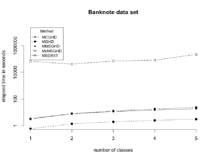
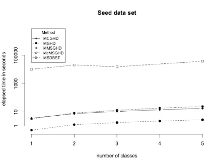
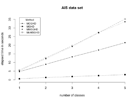
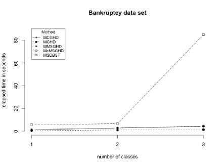
For the data sets listed in Table 4, we measured the elapsed user times, in seconds, to perform 100 (G)EM iterations. Note that all code was run in R version 3.0.2 on a 32-core Intel Xeon E5 server with 256GB RAM running 64-bit CentOS. Figure 4 displays the average elapsed time for two replications of each algorithm using a k𝑘k-means and a k𝑘k-medoids starting partition for G=1,,5𝐺15G=1,\ldots,5 components. The EM algorithm for the MSDBST is significantly slower than that of the hyperbolic-based approaches (Figure 4). In fact, on the banknote data set, it takes the MSDBST more than 11 hours to perform the required number of EM iterations when G=2𝐺2G=2 and about 63 hours when G=5𝐺5G=5. For the seeds data set, it takes the MSDBST more than 5 hours when G=2𝐺2G=2 and more than 10 hours when G=5𝐺5G=5, whereas the G=5𝐺5G=5 component MMSGHD, McMSGHD, and MCGHD approaches need less than 25 seconds. For the bankruptcy data set, the MSDBST requires approximately 80 seconds when G=3𝐺3G=3, whereas the hyperbolic distributions need less than 20 seconds each.
Refer to caption
Refer to caption
Refer to caption
Refer to caption
Figure 4: The average elapsed time to perform 100 iterations of the (G)EM algorithm when varying the number of components for MCGHD, MGHD, MMSGHD, McMSGHD, and MSDBST models on the bankruptcy, banknote, seeds, and AIS data sets, respectively.

7 Discussion

Novel MCGHDs, MMSGHDs, and McMSGHDs models have been introduced and applied for model-based clustering. The GHD is a flexible distribution, capable of handling skewness and heavy tails, and has many well known distributions as special or limiting cases. Furthermore, it is a normal variance-mean mixture, arising via a relationship between a multivariate Gaussian and an univariate GIG distribution. The MSGHD extends the GHD to include a multivariate GIG distribution, increasing the flexibility of the model. However, the GHD is not a special case of the MSGHD; hence, we created MCGHDs, which has both the GHD and MSGHD as special cases. The McMSGHD approach was introduced as a convex version of the MMSGHD, and this point deserves some further discussion. The extension of the multivariate-t𝑡t distribution to multiple scale was carried out by Forbes and Wraith (2014); as discussed in the Appendix B, the multiple scaled multivariate t𝑡t-distribution cannot be quasi-concave, i.e., the clusters associated with a mixture of multiple scaled multivariate t𝑡t-distributions cannot be convex. We have seen examples where the MMSGHD can put multiple clusters into one component, and the McMSGHD has an important role in helping to prevent this; if both approaches are fitted and lead to different numbers of components, then further attention is warranted.

Comparing the MGHD, MMSGHD, McMSGHD, and MCGHD approaches yielded some interesting results. Amongst them, we see that the MMSGHD does not necessarily outperform the MGHD; far from it, in fact, only the MGHD approach gave better clustering performance than the MMSGHD approach on one of the four real data sets we considered, as well as identical performance on a other two. This underlines the fact that a mixture of multiple scaled distributions may well not outperform its single scaled analogue, and highlights the benefit of approaches with both a multiple scaled distribution and its single scaled analogue as special cases. The MCGHDs represent one such approach, with the MSGHD and MGHD models as special cases. The approaches introduced herein, as well as the MGHDs, have been made freely available via the MixGHD package for R.

Future work will focus in several directions. For one, it will be interesting to study the performance of the approaches introduced herein within the fractionally-supervised classification framework (Vrbik and McNicholas, 2015; Gallaugher and McNicholas, 2019a). The extension of these approaches to the matrix-variate paradigm is also of interest and may proceed in an analogous fashion to the work of Gallaugher and McNicholas (2018, 2019b). Finally, the models introduced herein can be extended to account for missing data (see Wei et al., 2019).

Acknowledgements

This work was supported by a grant-in-aid from Compusense Inc., a Collaborative Research and Development Grant from the Natural Sciences and Engineering Research Council of Canada, and an Early Researcher Award from the Ontario Ministry of Research and Innovation.

References

  • Aitken (1926) Aitken, A. C. (1926). A series formula for the roots of algebraic and transcendental equations. Proceedings of the Royal Society of Edinburgh 45, 14–22.
  • Altman (1968) Altman, E. (1968). Financial ratios, discriminant analysis and the prediction of corporate bankruptcy. Journal of Finance 23(4), 589–609.
  • Andrews and McNicholas (2012) Andrews, J. L. and P. McNicholas (2012). Model-based clustering, classification, and discriminant analysis via mixtures of multivariate t𝑡t-distributions. Statistics and Computing 22(5), 1021–1029.
  • Andrews and McNicholas (2011a) Andrews, J. L. and P. D. McNicholas (2011a). Extending mixtures of multivariate t-factor analyzers. Statistics and Computing 21(3), 361–373.
  • Andrews and McNicholas (2011b) Andrews, J. L. and P. D. McNicholas (2011b). Mixtures of modified t-factor analyzers for model-based clustering, classification, and discriminant analysis. Journal of Statistical Planning and Inference 141(4), 1479–1486.
  • Azzalini et al. (2016) Azzalini, A., R. P. Browne, M. G. Genton, and P. D. McNicholas (2016). On nomenclature for, and the relative merits of, two formulations of skew distributions. Statistics and Probability Letters 110, 201–206.
  • Baek and McLachlan (2011) Baek, J. and G. J. McLachlan (2011). Mixtures of common t-factor analyzers for clustering high-dimensional microarray data. Bioinformatics 27, 1269–1276.
  • Banfield and Raftery (1993) Banfield, J. D. and A. E. Raftery (1993). Model-based Gaussian and non-Gaussian clustering. Biometrics 49(3), 803–821.
  • Barndorff-Nielsen (1978) Barndorff-Nielsen, O. (1978). Hyperbolic distributions and distributions on hyperbolae. Scandinavian Journal of Statistics 5(3), 151–157.
  • Barndorff-Nielsen et al. (1982) Barndorff-Nielsen, O., J. Kent, and M. Sørensen (1982). Normal variance-mean mixtures and z distributions. International Statistical Review / Revue Internationale de Statistique 50(2), 145–159.
  • Böhning et al. (1994) Böhning, D., E. Dietz, R. Schaub, P. Schlattmann, and B. Lindsay (1994). The distribution of the likelihood ratio for mixtures of densities from the one-parameter exponential family. Annals of the Institute of Statistical Mathematics 46, 373–388.
  • Browne and McNicholas (2014) Browne, R. P. and P. D. McNicholas (2014). Estimating common principal components in high dimensions. Advances in Data Analysis and Classification 8(2), 217–226.
  • Browne and McNicholas (2015) Browne, R. P. and P. D. McNicholas (2015). A mixture of generalized hyperbolic distributions. Canadian Journal of Statistics 43(2), 176–198.
  • Celeux and Govaert (1995) Celeux, G. and G. Govaert (1995). Gaussian parsimonious clustering models. Pattern Recognition 28(5), 781–793.
  • Charytanowicz et al. (2010) Charytanowicz, M., J. Niewczas, P. Kulczycki, P. A. Kowalski, S. Łukasik, and S. Żak (2010). A complete gradient clustering algorithm for features analysis of x-ray images. In E. Piȩtka and J. Kawa (Eds.), Information Technologies in Biomedicine: Volume 2, pp.  15–24. Berlin, Heidelberg: Springer.
  • Cook and Weisberg (1994) Cook, R. D. and S. Weisberg (1994). An Introduction to Regression Graphics. John Wiley & Sons, New York.
  • Cormack (1971) Cormack, R. M. (1971). A review of classification (with discussion). Journal of the Royal Statistical Society: Series A 34, 321–367.
  • Debreu and Koopmans (1982) Debreu, G. and T. C. Koopmans (1982). Additively decomposed quasiconvex functions. Mathematical Programming 24(1), 1–38.
  • Demarta and McNeil (2005) Demarta, S. and A. J. McNeil (2005). The t copula and related copulas. International Statistical Review 73(1), 111–129.
  • Dempster et al. (1977) Dempster, A. P., N. M. Laird, and D. B. Rubin (1977). Maximum likelihood from incomplete data via the EM algorithm. Journal of the Royal Statistical Society: Series B 39(1), 1–38.
  • Flury and Riedwyl (1988) Flury, B. and H. Riedwyl (1988). Multivariate Statistics: A Practical Approach. London: Chapman & Hall.
  • Forbes and Wraith (2014) Forbes, F. and D. Wraith (2014). A new family of multivariate heavy-tailed distributions with variable marginal amounts of tailweights: Application to robust clustering. Statistics and Computing 24(6), 971–984.
  • Fraley and Raftery (2002) Fraley, C. and A. E. Raftery (2002). Model-based clustering, discriminant analysis, and density estimation. Journal of the American Statistical Association 97(458), 611–631.
  • Franczak et al. (2014) Franczak, B. C., R. P. Browne, and P. D. McNicholas (2014). Mixtures of shifted asymmetric Laplace distributions. IEEE Transactions on Pattern Analysis and Machine Intelligence 36(6), 1149–1157.
  • Franczak et al. (2015) Franczak, B. C., C. Tortora, R. P. Browne, and P. D. McNicholas (2015). Unsupervised learning via mixtures of skewed distributions with hypercube contours. Pattern Recognition Letters 58(1), 69–76.
  • Gallaugher and McNicholas (2018) Gallaugher, M. P. B. and P. D. McNicholas (2018). Finite mixtures of skewed matrix variate distributions. Pattern Recognition 80, 83–93.
  • Gallaugher and McNicholas (2019a) Gallaugher, M. P. B. and P. D. McNicholas (2019a). On fractionally-supervised classification: Weight selection and extension to the multivariate t-distribution. Journal of Classification 36. In press.
  • Gallaugher and McNicholas (2019b) Gallaugher, M. P. B. and P. D. McNicholas (2019b). Three skewed matrix variate distributions. Statistics and Probability Letters 145, 103–109.
  • Ghahramani and Hinton (1997) Ghahramani, Z. and G. E. Hinton (1997). The EM algorithm for factor analyzers. Technical Report CRG-TR-96-1, University Of Toronto, Toronto.
  • Gneiting (1997) Gneiting, T. (1997). Normal scale mixtures and dual probability densities. Journal of Statistical Computation and Simulation 59(4), 375–384.
  • Hennig (2015) Hennig, C. (2015). What are the true clusters? Pattern Recognition Letters 63, 53–62.
  • Holzmann et al. (2006) Holzmann, H., A. Munk, and T. Gneiting (2006). Identifiability of finite mixtures of elliptical distributions. Scandinavian Journal of Statistics 33, 753–763.
  • Hubert and Arabie (1985) Hubert, L. and P. Arabie (1985). Comparing partitions. Journal of Classification 2(1), 193–218.
  • Hunter and Lange (2000) Hunter, D. R. and K. Lange (2000). Quantile regression via an MM algorithm. Journal of Computational and Graphical Statistics 9(1), 60–77.
  • Karlis and Santourian (2009) Karlis, D. and A. Santourian (2009). Model-based clustering with non-elliptically contoured distributions. Statistics and Computing 19(1), 73–83.
  • Kent (1983) Kent, J. T. (1983). Identifiability of finite mixtures for directional data. The Annals of Statistics 11, 984–988.
  • Kiers (2002) Kiers, H. A. (2002). Setting up alternating least squares and iterative majorization algorithms for solving various matrix optimization problems. Computational Statistics and Data Analysis 41(1), 157–170.
  • Kotz et al. (2001) Kotz, S., T. J. Kozubowski, and K. Podgorski (2001). The Laplace Distribution and Generalizations: A Revisit with Applications to Communications, Economics, Engineering, and Finance (1st ed.). Burkhauser Boston.
  • Kotz and Nadarajah (2004) Kotz, S. and S. Nadarajah (2004). Multivariate t-distributions and their applications. Cambridge University Press.
  • Lee and McLachlan (2013a) Lee, S. X. and G. J. McLachlan (2013a). EMMIXuskew: Fitting Unrestricted Multivariate Skew t Mixture Models. R package version 0.11-5.
  • Lee and McLachlan (2013b) Lee, S. X. and G. J. McLachlan (2013b). On mixtures of skew normal and skew t-distributions. Advances in Data Analysis and Classification 7(3), 241–266.
  • Lee and McLachlan (2014) Lee, S. X. and G. J. McLachlan (2014). Finite mixtures of multivariate skew t-distributions: some recent and new results. Statistics and Computing 24(2), 181–202.
  • Lin (2009) Lin, T. I. (2009). Maximum likelihood estimation for multivariate skew normal mixture models. Journal of Multivariate Analysis 100(2), 257–265.
  • Lin (2010) Lin, T. I. (2010). Robust mixture modeling using multivariate skew t distributions. Statistics and Computing 20(3), 343–356.
  • Lin et al. (2014) Lin, T.-I., P. D. McNicholas, and J. H. Hsiu (2014). Capturing patterns via parsimonious t mixture models. Statistics and Probability Letters 88, 80–87.
  • Lindsay (1995) Lindsay, B. (1995). Mixture models: Theory, geometry and applications. In NSF-CBMS Regional Conference Series in Probability and Statistics, Volume 5, California: Institute of Mathematical Statistics: Hayward.
  • McLachlan et al. (2007) McLachlan, G. J., R. W. Bean, and L. B.-T. Jones (2007). Extension of the mixture of factor analyzers model to incorporate the multivariate t-distribution. Computational Statistics and Data Analysis 51(11), 5327–5338.
  • McLachlan and Krishnan (2008) McLachlan, G. J. and T. Krishnan (2008). The EM Algorithm and Extensions. New York: Wiley.
  • McLachlan and Peel (2000) McLachlan, G. J. and D. Peel (2000). Mixtures of factor analyzers. In Proceedings of the Seventh International Conference on Machine Learning, San Francisco, pp.  599–606. Morgan Kaufmann.
  • McNeil et al. (2005) McNeil, A. J., R. Frey, and P. Embrechts (2005). Quantitative risk management: concepts, techniques and tools. Princeton university press.
  • McNicholas (2016a) McNicholas, P. D. (2016a). Mixture Model-Based Classification. Boca-Raton: Chapman & Hall/CRC press.
  • McNicholas (2016b) McNicholas, P. D. (2016b). Model-based clustering. Journal of Classification 33(3), 331–373.
  • McNicholas et al. (2010) McNicholas, P. D., T. B. Murphy, A. F. McDaid, and D. Frost (2010). Serial and parallel implementations of model-based clustering via parsimonious Gaussian mixture models. Computational Statistics and Data Analysis 54(3), 711–723.
  • McNicholas et al. (2017) McNicholas, S. M., P. D. McNicholas, and R. P. Browne (2017). A mixture of variance-gamma factor analyzers. In S. E. Ahmed (Ed.), Big and Complex Data Analysis: Methodologies and Applications, pp.  369–385. Cham: Springer International Publishing.
  • Murray et al. (2014) Murray, P. M., R. B. Browne, and P. D. McNicholas (2014). Mixtures of skew-t factor analyzers. Computational Statistics and Data Analysis 77, 326–335.
  • Murray et al. (2017) Murray, P. M., R. B. Browne, and P. D. McNicholas (2017). Hidden truncation hyperbolic distributions, finite mixtures thereof, and their application for clustering. Journal of Multivariate Analysis 161, 141–156.
  • Niculescu and Persson (2006) Niculescu, C. and L. Persson (2006). Convex Functions and Their Applications. New York: Springer.
  • Ortega and Rheinboldt (1970) Ortega, J. M. and W. C. Rheinboldt (1970). Iterative Solutions of Nonlinear Equations in Several Variables. New York: Academic Press.
  • Peel and McLachlan (2000) Peel, D. and G. J. McLachlan (2000). Robust mixture modelling using the t distribution. Statistics and Computing 10(4), 339–348.
  • Pesevski et al. (2018) Pesevski, A., B. C. Franczak, and P. D. McNicholas (2018). Subspace clustering with the multivariate-t distribution. Pattern Recognition Letters 112(1), 297–302.
  • R Core Team (2017) R Core Team (2017). R: A Language and Environment for Statistical Computing. Vienna, Austria: R Foundation for Statistical Computing.
  • Rand (1971) Rand, W. M. (1971). Objective criteria for the evaluation of clustering methods. Journal of the American Statistical Association 66(336), 846–850.
  • Rockafellar and Wets (2009) Rockafellar, R. T. and R. J. B. Wets (2009). Variational Analysis. New York: Springer-Verlag.
  • Schwarz (1978) Schwarz, G. (1978). Estimating the dimension of a model. Annals of Statistics 6(2), 461–464.
  • Steane et al. (2012) Steane, M. A., P. D. McNicholas, and R. Yada (2012). Model-based classification via mixtures of multivariate t-factor analyzers. Communications in Statistics – Simulation and Computation 41(4), 510–523.
  • Steinley (2004) Steinley, D. (2004). Properties of the Hubert-Arable adjusted Rand index. Psychological methods 9(3), 386.
  • Tang et al. (2018) Tang, Y., R. P. Browne, and P. D. McNicholas (2018). Flexible clustering of high-dimensional data via mixtures of joint generalized hyperbolic distributions. Stat 7(1), e177.
  • Tipping and Bishop (1999) Tipping, M. E. and C. M. Bishop (1999). Mixtures of probabilistic principal component analysers. Neural Computation 11(2), 443–482.
  • Tortora et al. (2017) Tortora, C., R. P. Browne, B. C. Franczak, and P. D. McNicholas (2017). MixGHD: Model based clustering, classification and discriminant analysis using the mixture of generalized hyperbolic distributions. R package version 2.1.
  • Vrbik and McNicholas (2012) Vrbik, I. and P. D. McNicholas (2012). Analytic calculations for the EM algorithm for multivariate skew-mixture models. Statistics and Probability Letters 82(6), 1169–1174.
  • Vrbik and McNicholas (2014) Vrbik, I. and P. D. McNicholas (2014). Parsimonious skew mixture models for model-based clustering and classification. Computational Statistics and Data Analysis 71, 196–210.
  • Vrbik and McNicholas (2015) Vrbik, I. and P. D. McNicholas (2015). Fractionally-supervised classification. Journal of Classification 32(3), 359–381.
  • Wei et al. (2019) Wei, Y., Y. Tang, and P. D. McNicholas (2019). Mixtures of generalized hyperbolic distributions and mixtures of skew-t distributions for model-based clustering with incomplete data. Computational Statistics and Data Analysis 130, 18–41.
  • Wraith and Forbes (2015) Wraith, D. and F. Forbes (2015). Clustering using skewed multivariate heavy tailed distributions with flexible tail behaviour. arXiv preprint arXiv:1408.0711.
  • Yakowitz and Spragins (1968) Yakowitz, S. J. and J. Spragins (1968). On the identifiability of finite mixtures. Ann. Math. Statist. 39, 209–214.

Appendix A Parameter estimation

We use the EM algorithm to estimate the parameters of the MCGHDs. The EM algorithm belongs to a larger class of algorithms known as MM algorithms (Ortega and Rheinboldt, 1970; Hunter and Lange, 2000) and is well-suited for problems involving missing data. ‘MM’ stands for ‘minorize-maximize’ or ‘majorize-minimize,’ depending on the purpose of the algorithm; in the EM context, the minorizing function is the expected value of the complete-data log-likelihood. The EM algorithm iterates between two steps, an E-step and a M-step, and has been used to estimate the parameters of mixture models in many experiments (McLachlan and Krishnan, 2008). On each E-step, the expected value of the complete-data log-likelihood, 𝒬𝒬\mathcal{Q}, is calculated and on each M-step is maximized with respect to πg,𝝁g,𝚽g,𝜶g,𝝎g,𝝀g,ω0g,λ0g,ϖgsubscript𝜋𝑔subscript𝝁𝑔subscript𝚽𝑔subscript𝜶𝑔subscript𝝎𝑔subscript𝝀𝑔subscript𝜔0𝑔subscript𝜆0𝑔subscriptitalic-ϖ𝑔\pi_{g},\mbox{\boldmath$\mu$}_{g},\mathbf{\Phi}_{g},\mbox{\boldmath$\alpha$}_{g},\mbox{\boldmath$\omega$}_{g},\mbox{\boldmath$\lambda$}_{g},\omega_{0g},\lambda_{0g},\varpi_{g}. However, in each M-step 𝒬𝒬\mathcal{Q} increases with respect to 𝚪gsubscript𝚪𝑔\mathbf{\Gamma}_{g} rather than maximize; accordingly, the algorithm is formally a generalized EM (GEM) algorithm. For our MCGHDs, there are four sources of missing data: the latent variable W0igsubscript𝑊0𝑖𝑔W_{0ig}, the multi-dimensional weight variable 𝚫𝐰igsubscript𝚫𝐰𝑖𝑔\mathbf{\Delta}_{\mathbf{w}ig}, the group component indicator labels zigsubscript𝑧𝑖𝑔z_{ig}, and inner component labels uigsubscript𝑢𝑖𝑔u_{ig}, for i=1,,n𝑖1𝑛i=1,\ldots,n and g=1,,G𝑔1𝐺g=1,\ldots,G. For each observation i𝑖i, zig=1subscript𝑧𝑖𝑔1z_{ig}=1 if observation i𝑖i is in component g𝑔g and zig=0subscript𝑧𝑖𝑔0z_{ig}=0 otherwise. Similarly, for each observation i𝑖i, uig=1subscript𝑢𝑖𝑔1u_{ig}=1 if observation i𝑖i, in component g𝑔g, is distributed generalized hyperbolic and uig=0subscript𝑢𝑖𝑔0u_{ig}=0 if observation i𝑖i, in component g𝑔g, is distributed multiple scaled generalized hyperbolic. It follows that the complete-data log-likelihood for the MCGHDs is given by

lc=i=1ng=1G{ziglogπg+ziguiglogϖg+zig(1uig)log(1ϖg)+ziguiglogh(w0ig|ω0g,1,λ0g)+zig(1uig)j=1plogh(wjig|ωjg,1,λjg)+ziguiglogϕp(𝚪g𝐱i|𝝁g+w0ig𝜶g,w0ig𝚽)+zig(1uig)j=1plogϕ1([𝚪g𝐱i]j|μjg+wjigαjg,ωjgϕjg)},subscript𝑙𝑐superscriptsubscript𝑖1𝑛superscriptsubscript𝑔1𝐺subscript𝑧𝑖𝑔subscript𝜋𝑔subscript𝑧𝑖𝑔subscript𝑢𝑖𝑔subscriptitalic-ϖ𝑔subscript𝑧𝑖𝑔1subscript𝑢𝑖𝑔1subscriptitalic-ϖ𝑔subscript𝑧𝑖𝑔subscript𝑢𝑖𝑔|subscript𝑤0𝑖𝑔subscript𝜔0𝑔1subscript𝜆0𝑔subscript𝑧𝑖𝑔1subscript𝑢𝑖𝑔superscriptsubscript𝑗1𝑝conditionalsubscript𝑤𝑗𝑖𝑔subscript𝜔𝑗𝑔1subscript𝜆𝑗𝑔subscript𝑧𝑖𝑔subscript𝑢𝑖𝑔subscriptitalic-ϕ𝑝conditionalsuperscriptsubscript𝚪𝑔subscript𝐱𝑖subscript𝝁𝑔subscript𝑤0𝑖𝑔subscript𝜶𝑔subscript𝑤0𝑖𝑔𝚽subscript𝑧𝑖𝑔1subscript𝑢𝑖𝑔superscriptsubscript𝑗1𝑝subscriptitalic-ϕ1|subscriptdelimited-[]superscriptsubscript𝚪𝑔subscript𝐱𝑖𝑗subscript𝜇𝑗𝑔subscript𝑤𝑗𝑖𝑔subscript𝛼𝑗𝑔subscript𝜔𝑗𝑔subscriptitalic-ϕ𝑗𝑔\begin{split}l_{c}&=\sum_{i=1}^{n}\sum_{g=1}^{G}\bigg{\{}z_{ig}\log\pi_{g}+z_{ig}{u_{ig}}\log\varpi_{g}+z_{ig}(1-u_{ig})\log(1-\varpi_{g})+z_{ig}{u_{ig}}\log h\left(w_{0ig}~{}|~{}\omega_{0g},1,\lambda_{0g}\right)\\ &+z_{ig}(1-u_{ig})\sum_{j=1}^{p}\log h\left(w_{jig}~{}|~{}\omega_{jg},1,\lambda_{jg}\right)+z_{ig}{u_{ig}}\log\phi_{p}\left(\mathbf{\Gamma}_{g}^{\prime}\mathbf{x}_{i}~{}|~{}\mbox{\boldmath$\mu$}_{g}+w_{0ig}\mbox{\boldmath$\alpha$}_{g},w_{0ig}\mathbf{\Phi}\right)\\ &+z_{ig}(1-u_{ig})\sum_{j=1}^{p}\log\phi_{1}\left([\mathbf{\Gamma}_{g}^{\prime}\mathbf{x}_{i}]_{j}~{}|~{}\mu_{jg}+w_{jig}\alpha_{jg},\omega_{jg}\phi_{jg}\right)\bigg{\}},\end{split}

where ϕp()subscriptitalic-ϕ𝑝\phi_{p}(\cdot) represents a p𝑝p-dimensional Gaussian density function, ϕ1()subscriptitalic-ϕ1\phi_{1}(\cdot) is a unidimensional Gaussian density function, and h()h(\cdot) is the density of a GIG distribution given in (15).

We are now prepared to outline the calculations for our GEM algorithm for the MCGHDs. On the E-step, the expected value of the complete-data log-likelihood,𝒬𝒬~{}\mathcal{Q}, is computed by replacing the sufficient statistics of the missing data by their expected values. For each component indicator label zigsubscript𝑧𝑖𝑔z_{ig} and inner component label uigsubscript𝑢𝑖𝑔u_{ig}, for i=1,,n𝑖1𝑛i=1,\ldots,n and g=1,,G𝑔1𝐺g=1,\ldots,G, we require the expectations

𝔼[Zig𝐱i]=πgfCGHD(𝐱𝝁g,𝚪g,𝚽g,𝜶g,𝝎g,𝝀g,ω0g,λ0g,ϖg)h=1GπhfCGHD(𝐱𝝁h,𝚪h,𝚽h,𝜶h,𝝎h,𝝀h,ω0h,λ0h,ϖh)\equalscolonz^ig𝔼delimited-[]conditionalsubscript𝑍𝑖𝑔subscript𝐱𝑖subscript𝜋𝑔subscript𝑓CGHDconditional𝐱subscript𝝁𝑔subscript𝚪𝑔subscript𝚽𝑔subscript𝜶𝑔subscript𝝎𝑔subscript𝝀𝑔subscript𝜔0𝑔subscript𝜆0𝑔subscriptitalic-ϖ𝑔superscriptsubscript1𝐺subscript𝜋subscript𝑓CGHDconditional𝐱subscript𝝁subscript𝚪subscript𝚽subscript𝜶subscript𝝎subscript𝝀subscript𝜔0subscript𝜆0subscriptitalic-ϖ\equalscolonsubscript^𝑧𝑖𝑔\mathbb{E}\left[Z_{ig}\mid\mathbf{x}_{i}\right]=\frac{\pi_{g}f_{\text{\tiny CGHD}}\left(\mathbf{x}\mid\mbox{\boldmath$\mu$}_{g},\mathbf{\Gamma}_{g},\mathbf{\Phi}_{g},\mbox{\boldmath$\alpha$}_{g},\mbox{\boldmath$\omega$}_{g},\mbox{\boldmath$\lambda$}_{g},\omega_{0g},\lambda_{0g},\varpi_{g}\right)}{\sum_{h=1}^{G}\pi_{h}f_{\text{\tiny CGHD}}\left(\mathbf{x}\mid\mbox{\boldmath$\mu$}_{h},\mathbf{\Gamma}_{h},\mathbf{\Phi}_{h},\mbox{\boldmath$\alpha$}_{h},\mbox{\boldmath$\omega$}_{h},\mbox{\boldmath$\lambda$}_{h},\omega_{0h},\lambda_{0h},\varpi_{h}\right)}\equalscolon\hat{z}_{ig} (21)

and

𝔼[Uig𝐱i,zig=1]=ϖgfGHD(𝐱𝝁g,𝚪g𝚽g𝚪g,𝜶g,ω0g,λ0g)ϖgfGHD(𝐱𝝁g,𝚪g𝚽g𝚪g,𝜶g,ω0g,λ0g)+(1ϖg)fMSGHD(𝐱𝝁g,𝚪g,𝚽g,𝜶g,𝝎g,𝝀g)\equalscolonu^ig,𝔼delimited-[]conditionalsubscript𝑈𝑖𝑔subscript𝐱𝑖subscript𝑧𝑖𝑔1subscriptitalic-ϖ𝑔subscript𝑓GHDconditional𝐱subscript𝝁𝑔subscript𝚪𝑔subscript𝚽𝑔superscriptsubscript𝚪𝑔subscript𝜶𝑔subscript𝜔0𝑔subscript𝜆0𝑔subscriptitalic-ϖ𝑔subscript𝑓GHDconditional𝐱subscript𝝁𝑔subscript𝚪𝑔subscript𝚽𝑔superscriptsubscript𝚪𝑔subscript𝜶𝑔subscript𝜔0𝑔subscript𝜆0𝑔1subscriptitalic-ϖ𝑔subscript𝑓MSGHDconditional𝐱subscript𝝁𝑔subscript𝚪𝑔subscript𝚽𝑔subscript𝜶𝑔subscript𝝎𝑔subscript𝝀𝑔\equalscolonsubscript^𝑢𝑖𝑔\begin{split}&\mathbb{E}\left[U_{ig}\mid\mathbf{x}_{i},z_{ig}=1\right]=\\ &\qquad\frac{\varpi_{g}f_{\text{\tiny GHD}}(\mathbf{x}\mid\mbox{\boldmath$\mu$}_{g},\mathbf{\Gamma}_{g}\mathbf{\Phi}_{g}\mathbf{\Gamma}_{g}^{\prime},\mbox{\boldmath$\alpha$}_{g},\omega_{0g},\lambda_{0g})}{\varpi_{g}f_{\text{\tiny GHD}}(\mathbf{x}\mid\mbox{\boldmath$\mu$}_{g},\mathbf{\Gamma}_{g}\mathbf{\Phi}_{g}\mathbf{\Gamma}_{g}^{\prime},\mbox{\boldmath$\alpha$}_{g},\omega_{0g},\lambda_{0g})+(1-\varpi_{g})f_{\text{\tiny MSGHD}}\left(\mathbf{x}\mid\mbox{\boldmath$\mu$}_{g},\mathbf{\Gamma}_{g},\mathbf{\Phi}_{g},\mbox{\boldmath$\alpha$}_{g},\mbox{\boldmath$\omega$}_{g},\mbox{\boldmath$\lambda$}_{g}\right)}\equalscolon\hat{u}_{ig},\end{split} (22)

where fCGHDsubscript𝑓CGHDf_{\tiny\text{CGHD}} is given in (20), fGHDsubscript𝑓GHDf_{\tiny\text{GHD}} is given in (10) and fMSGHDsubscript𝑓MSGHDf_{\tiny\text{MSGHD}} is given in (17). For the latent variable W0igsubscript𝑊0𝑖𝑔W_{0ig}, we use the expected value given in Browne and McNicholas (2015). The authors show that, given the density in (15), the following is true

W0ig𝐱i,zig=1,uig=1𝒢𝒢(ω0g+𝜶g(𝚪g𝚽g𝚪g)1𝜶g,ω0g+δ(𝐱i,𝝁g𝚪g𝚽g𝚪g),λ0gp/2).formulae-sequenceconditionalsubscript𝑊0𝑖𝑔subscript𝐱𝑖subscript𝑧𝑖𝑔1subscript𝑢𝑖𝑔1𝒢𝒢subscript𝜔0𝑔superscriptsubscript𝜶𝑔superscriptsubscript𝚪𝑔subscript𝚽𝑔superscriptsubscript𝚪𝑔1subscript𝜶𝑔subscript𝜔0𝑔𝛿subscript𝐱𝑖conditionalsubscript𝝁𝑔subscript𝚪𝑔subscript𝚽𝑔superscriptsubscript𝚪𝑔subscript𝜆0𝑔𝑝2W_{0ig}\mid\mathbf{x}_{i},z_{ig}=1,u_{ig}=1\backsim\mathcal{GIG}\left(\omega_{0g}+\mbox{\boldmath$\alpha$}_{g}^{\prime}(\mathbf{\Gamma}_{g}\mathbf{\Phi}_{g}\mathbf{\Gamma}_{g}^{\prime})^{-1}\mbox{\boldmath$\alpha$}_{g},\omega_{0g}+\delta(\mathbf{x}_{i},\mbox{\boldmath$\mu$}_{g}\mid\mathbf{\Gamma}_{g}\mathbf{\Phi}_{g}\mathbf{\Gamma}_{g}^{\prime}),\lambda_{0g}-p/2\right).

For the MCGHDs, the maximization of 𝒬𝒬\mathcal{Q} requires the expected values of W0igsubscript𝑊0𝑖𝑔W_{0ig}, W0ig1subscriptsuperscript𝑊10𝑖𝑔W^{-1}_{0ig} and logW0igsubscript𝑊0𝑖𝑔\log W_{0ig}, i.e.,

𝔼[W0ig|𝐱i,zig=1,uig=1]=eigdgKλ0gp/2+1(dgeig)Kλ0gp/2(dgeig)\equalscolonaig,𝔼delimited-[]formulae-sequenceconditionalsubscript𝑊0𝑖𝑔subscript𝐱𝑖subscript𝑧𝑖𝑔1subscript𝑢𝑖𝑔1subscript𝑒𝑖𝑔subscript𝑑𝑔subscript𝐾subscript𝜆0𝑔𝑝21subscript𝑑𝑔subscript𝑒𝑖𝑔subscript𝐾subscript𝜆0𝑔𝑝2subscript𝑑𝑔subscript𝑒𝑖𝑔\equalscolonsubscript𝑎𝑖𝑔\displaystyle{\mathbb{E}}[W_{0ig}~{}|~{}\mathbf{x}_{i},z_{ig}=1,u_{ig}=1]=\sqrt{\frac{e_{ig}}{d_{g}}}\frac{K_{\lambda_{0g}-p/2+1}\left(\sqrt{d_{g}e_{ig}}\right)}{K_{\lambda_{0g}-p/2}\left(\sqrt{d_{g}e_{ig}}\right)}\equalscolon a_{ig},
𝔼[W0ig1|𝐱i,zig=1,uig=1]=dgeigKλ0gp/2+1(dgeig)Kλ0gp/2(dgeig)2λ0gpeig\equalscolonbig,𝔼delimited-[]formulae-sequenceconditionalsuperscriptsubscript𝑊0𝑖𝑔1subscript𝐱𝑖subscript𝑧𝑖𝑔1subscript𝑢𝑖𝑔1subscript𝑑𝑔subscript𝑒𝑖𝑔subscript𝐾subscript𝜆0𝑔𝑝21subscript𝑑𝑔subscript𝑒𝑖𝑔subscript𝐾subscript𝜆0𝑔𝑝2subscript𝑑𝑔subscript𝑒𝑖𝑔2subscript𝜆0𝑔𝑝subscript𝑒𝑖𝑔\equalscolonsubscript𝑏𝑖𝑔\displaystyle{\mathbb{E}}[W_{0ig}^{-1}~{}|~{}\mathbf{x}_{i},z_{ig}=1,u_{ig}=1]=\sqrt{\frac{d_{g}}{e_{ig}}}\frac{K_{\lambda_{0g}-p/2+1}\left(\sqrt{d_{g}e_{ig}}\right)}{K_{\lambda_{0g}-p/2}\left(\sqrt{d_{g}e_{ig}}\right)}-\frac{2\lambda_{0g}-p}{e_{ig}}\equalscolon b_{ig},
𝔼[logW0ig|𝐱i,zig=1,uig=1]=logeigdg+vlog{Kv(dgeig)}|v=λ0gp/2\equalscoloncig,𝔼delimited-[]formulae-sequenceconditionalsubscript𝑊0𝑖𝑔subscript𝐱𝑖subscript𝑧𝑖𝑔1subscript𝑢𝑖𝑔1subscript𝑒𝑖𝑔subscript𝑑𝑔evaluated-at𝑣subscript𝐾𝑣subscript𝑑𝑔subscript𝑒𝑖𝑔𝑣subscript𝜆0𝑔𝑝2\equalscolonsubscript𝑐𝑖𝑔\displaystyle{\mathbb{E}}[\log W_{0ig}~{}|~{}\mathbf{x}_{i},z_{ig}=1,u_{ig}=1]=\log\sqrt{\frac{e_{ig}}{d_{g}}}+\left.\frac{\partial}{\partial v}\log\left\{K_{v}\left(\sqrt{d_{g}e_{ig}}\right)\right\}\right|_{v=\lambda_{0g}-p/2}\equalscolon c_{ig},

where dg=ω0g+𝜶g(𝚪g𝚽g𝚪g)1𝜶gsubscript𝑑𝑔subscript𝜔0𝑔superscriptsubscript𝜶𝑔superscriptsubscript𝚪𝑔subscript𝚽𝑔subscriptsuperscript𝚪𝑔1subscript𝜶𝑔d_{g}=\omega_{0g}+\mbox{\boldmath$\alpha$}_{g}^{\prime}(\mathbf{\Gamma}_{g}\mathbf{\Phi}_{g}\mathbf{\Gamma}^{\prime}_{g})^{-1}\mbox{\boldmath$\alpha$}_{g} and eig=ω0g+δ(𝐱i,𝝁g𝚪g𝚽g𝚪g)subscript𝑒𝑖𝑔subscript𝜔0𝑔𝛿subscript𝐱𝑖conditionalsubscript𝝁𝑔subscript𝚪𝑔subscript𝚽𝑔subscriptsuperscript𝚪𝑔e_{ig}=\omega_{0g}+\delta(\mathbf{x}_{i},\mbox{\boldmath$\mu$}_{g}\mid\mathbf{\Gamma}_{g}\mathbf{\Phi}_{g}\mathbf{\Gamma}^{\prime}_{g}).

The maximization of 𝒬𝒬\mathcal{Q} also requires the expected values of the multidimensional weight variables 𝚫𝐰igsubscript𝚫𝐰𝑖𝑔\mathbf{\Delta}_{\mathbf{w}ig}, 𝚫𝐰ig1superscriptsubscript𝚫𝐰𝑖𝑔1\mathbf{\Delta}_{\mathbf{w}ig}^{-1}, and log𝚫𝐰igsubscript𝚫𝐰𝑖𝑔\log\mathbf{\Delta}_{\mathbf{w}ig}. Given the density in (17), it follows that

Wijg|𝐱i,zig=1,uig=0𝒢𝒢(ωjg+αjg2Φjg1,ωjg+([𝚪𝐱]j𝝁gj)2/ϕjg,λjg1/2).formulae-sequenceconditionalsubscript𝑊𝑖𝑗𝑔subscript𝐱𝑖subscript𝑧𝑖𝑔1subscript𝑢𝑖𝑔0𝒢𝒢subscript𝜔𝑗𝑔superscriptsubscript𝛼𝑗𝑔2superscriptsubscriptΦ𝑗𝑔1subscript𝜔𝑗𝑔superscriptsubscriptdelimited-[]superscript𝚪𝐱𝑗subscript𝝁𝑔𝑗2subscriptitalic-ϕ𝑗𝑔subscript𝜆𝑗𝑔12W_{ijg}~{}|~{}\mathbf{x}_{i},z_{ig}=1,u_{ig}=0\backsim\mathcal{GIG}\left(\omega_{jg}+\alpha_{jg}^{2}\Phi_{jg}^{-1},\omega_{jg}+({\left[\mathbf{\Gamma}^{\prime}\mathbf{x}\right]_{j}}-\mbox{\boldmath$\mu$}_{gj})^{2}/\phi_{jg},\lambda_{jg}-1/2\right).

Each multidimensional weight variable is replaced by its expected value and so we need to compute 𝐄1ig=diag{E1i1g,,E1ipg}subscript𝐄1𝑖𝑔diagsubscript𝐸1𝑖1𝑔subscript𝐸1𝑖𝑝𝑔{\mathbf{E}}_{1ig}=\,\mbox{diag}\{E_{1i1g},\ldots,E_{1ipg}\}, 𝐄2ig=diag{E2i1g,,E2ipg}subscript𝐄2𝑖𝑔diagsubscript𝐸2𝑖1𝑔subscript𝐸2𝑖𝑝𝑔{\mathbf{E}}_{2ig}=\,\mbox{diag}\{E_{2i1g},\ldots,E_{2ipg}\}, and 𝐄3ig=diag{E3i1g,,E3ipg}subscript𝐄3𝑖𝑔diagsubscript𝐸3𝑖1𝑔subscript𝐸3𝑖𝑝𝑔{\mathbf{E}}_{3ig}=\,\mbox{diag}\{E_{3i1g},\ldots,E_{3ipg}\}, where

𝔼[Wijg𝐱i,zig=1,uig=0]=e¯ijgd¯jgKλjg+1/2(d¯jge¯ijg)Kλjg1/2(d¯jge¯ijg)\equalscolonE1ijg,𝔼[Wijg1𝐱i,zig=1,uig=0]=d¯jge¯ijgKλjg+1/2(d¯jge¯ijg)Kλjg1/2(d¯jge¯ijg)2λjg1e¯ijg\equalscolonE2ijg,𝔼[logWijg𝐱i,zig=1,uig=0]=loge¯ijgd¯jg+vlog{Kv(d¯jge¯ijg)}|v=λjg1/2\equalscolonE3ijg,formulae-sequence𝔼delimited-[]formulae-sequenceconditionalsubscript𝑊𝑖𝑗𝑔subscript𝐱𝑖subscript𝑧𝑖𝑔1subscript𝑢𝑖𝑔0subscript¯𝑒𝑖𝑗𝑔subscript¯𝑑𝑗𝑔subscript𝐾subscript𝜆𝑗𝑔12subscript¯𝑑𝑗𝑔subscript¯𝑒𝑖𝑗𝑔subscript𝐾subscript𝜆𝑗𝑔12subscript¯𝑑𝑗𝑔subscript¯𝑒𝑖𝑗𝑔\equalscolonsubscript𝐸1𝑖𝑗𝑔formulae-sequence𝔼delimited-[]formulae-sequenceconditionalsuperscriptsubscript𝑊𝑖𝑗𝑔1subscript𝐱𝑖subscript𝑧𝑖𝑔1subscript𝑢𝑖𝑔0subscript¯𝑑𝑗𝑔subscript¯𝑒𝑖𝑗𝑔subscript𝐾subscript𝜆𝑗𝑔12subscript¯𝑑𝑗𝑔subscript¯𝑒𝑖𝑗𝑔subscript𝐾subscript𝜆𝑗𝑔12subscript¯𝑑𝑗𝑔subscript¯𝑒𝑖𝑗𝑔2subscript𝜆𝑗𝑔1subscript¯𝑒𝑖𝑗𝑔\equalscolonsubscript𝐸2𝑖𝑗𝑔𝔼delimited-[]formulae-sequenceconditionalsubscript𝑊𝑖𝑗𝑔subscript𝐱𝑖subscript𝑧𝑖𝑔1subscript𝑢𝑖𝑔0subscript¯𝑒𝑖𝑗𝑔subscript¯𝑑𝑗𝑔evaluated-at𝑣subscript𝐾𝑣subscript¯𝑑𝑗𝑔subscript¯𝑒𝑖𝑗𝑔𝑣subscript𝜆𝑗𝑔12\equalscolonsubscript𝐸3𝑖𝑗𝑔\begin{split}&\mathbb{E}[W_{ijg}\mid\mathbf{x}_{i},z_{ig}=1,u_{ig}=0]=\sqrt{\frac{\bar{e}_{ijg}}{\bar{d}_{jg}}}\frac{K_{\lambda_{jg}+1/2}\left(\sqrt{\bar{d}_{jg}\bar{e}_{ijg}}\right)}{K_{\lambda_{jg}-1/2}\left(\sqrt{\bar{d}_{jg}\bar{e}_{ijg}}\right)}\equalscolon E_{1ijg},\\ &\mathbb{E}[W_{ijg}^{-1}\mid\mathbf{x}_{i},z_{ig}=1,u_{ig}=0]=\sqrt{\frac{\bar{d}_{jg}}{\bar{e}_{ijg}}}\frac{K_{\lambda_{jg}+1/2}\left(\sqrt{\bar{d}_{jg}\bar{e}_{ijg}}\right)}{K_{\lambda_{jg}-1/2}\left(\sqrt{\bar{d}_{jg}\bar{e}_{ijg}}\right)}-\frac{2\lambda_{jg}-1}{\bar{e}_{ijg}}\equalscolon E_{2ijg},\\ &\mathbb{E}[\log W_{ijg}\mid\mathbf{x}_{i},z_{ig}=1,u_{ig}=0]=\log\sqrt{\frac{\bar{e}_{ijg}}{\bar{d}_{jg}}}+\frac{\partial}{\partial v}\left.\log\left\{K_{v}\left(\sqrt{\bar{d}_{jg}\bar{e}_{ijg}}\right)\right\}\right|_{v=\lambda_{jg}-1/2}\equalscolon E_{3ijg},\end{split} (23)

d¯jg=ωjg+αjg2Φjg1subscript¯𝑑𝑗𝑔subscript𝜔𝑗𝑔superscriptsubscript𝛼𝑗𝑔2superscriptsubscriptΦ𝑗𝑔1\bar{d}_{jg}=\omega_{jg}+\alpha_{jg}^{2}\Phi_{jg}^{-1} and e¯ijg=ωjg+([𝐱i𝝁g]j)2/ϕjgsubscript¯𝑒𝑖𝑗𝑔subscript𝜔𝑗𝑔superscriptsubscriptdelimited-[]subscript𝐱𝑖subscript𝝁𝑔𝑗2subscriptitalic-ϕ𝑗𝑔\bar{e}_{ijg}=\omega_{jg}+([\mathbf{x}_{i}-\mbox{\boldmath$\mu$}_{g}]_{j})^{2}/\phi_{jg}. Let ng=i=1nz^igsubscript𝑛𝑔superscriptsubscript𝑖1𝑛subscript^𝑧𝑖𝑔n_{g}=\sum_{i=1}^{n}\hat{z}_{ig}, Ag=(1/ng)i=1nz^igaigsubscript𝐴𝑔1subscript𝑛𝑔superscriptsubscript𝑖1𝑛subscript^𝑧𝑖𝑔subscript𝑎𝑖𝑔A_{g}=(1/n_{g})\sum_{i=1}^{n}\hat{z}_{ig}a_{ig}, Bg=(1/ng)i=1nz^igbigsubscript𝐵𝑔1subscript𝑛𝑔superscriptsubscript𝑖1𝑛subscript^𝑧𝑖𝑔subscript𝑏𝑖𝑔B_{g}=(1/n_{g})\sum_{i=1}^{n}\hat{z}_{ig}b_{ig}, Cg=(1/ng)i=1nz^igcigsubscript𝐶𝑔1subscript𝑛𝑔superscriptsubscript𝑖1𝑛subscript^𝑧𝑖𝑔subscript𝑐𝑖𝑔C_{g}=(1/n_{g})\sum_{i=1}^{n}\hat{z}_{ig}c_{ig}, E¯1jg=(1/ng)i=1nz^igE1ijgsubscript¯𝐸1𝑗𝑔1subscript𝑛𝑔superscriptsubscript𝑖1𝑛subscript^𝑧𝑖𝑔subscript𝐸1𝑖𝑗𝑔{\bar{E}}_{1jg}=(1/n_{g})\sum_{i=1}^{n}\hat{z}_{ig}{E}_{1ijg}, E¯2jg=(1/ng)i=1nz^igE2ijgsubscript¯𝐸2𝑗𝑔1subscript𝑛𝑔superscriptsubscript𝑖1𝑛subscript^𝑧𝑖𝑔subscript𝐸2𝑖𝑗𝑔{\bar{E}}_{2jg}=(1/n_{g})\sum_{i=1}^{n}\hat{z}_{ig}{E}_{2ijg}, and E¯3jg=(1/ng)i=1nz^igE3ijgsubscript¯𝐸3𝑗𝑔1subscript𝑛𝑔superscriptsubscript𝑖1𝑛subscript^𝑧𝑖𝑔subscript𝐸3𝑖𝑗𝑔{\bar{E}}_{3jg}=(1/n_{g})\sum_{i=1}^{n}\hat{z}_{ig}{E}_{3ijg}.

In the M-step, we maximize the expected value of the complete-data log-likelihood with respect to the model parameters. The mixing proportions and inner mixing proportions are updated via π^g=ng/nsubscript^𝜋𝑔subscript𝑛𝑔𝑛\hat{\pi}_{g}=n_{g}/n and ϖ^g=i=1nu^igz^ig/ngsubscript^italic-ϖ𝑔superscriptsubscript𝑖1𝑛subscript^𝑢𝑖𝑔subscript^𝑧𝑖𝑔subscript𝑛𝑔\hat{\varpi}_{g}={\sum_{i=1}^{n}\hat{u}_{ig}\hat{z}_{ig}}/{n_{g}}, respectively. The elements of the location parameter 𝝁gsubscript𝝁𝑔\mbox{\boldmath$\mu$}_{g} and skewness parameter 𝜶gsubscript𝜶𝑔\mbox{\boldmath$\alpha$}_{g} are replaced with

μ^jg=i=1nz^ig[𝚪g𝐱i]j(s¯1jgs2ijg1)i=1nz^ig(s¯1jgs2ijg1)andα^jg=i=1nz^ig[𝚪g𝐱i]j(s¯2jgs2ijg)i=1nz^ig(s¯1jgs2ijg1),subscript^𝜇𝑗𝑔superscriptsubscript𝑖1𝑛subscript^𝑧𝑖𝑔subscriptdelimited-[]superscriptsubscript𝚪𝑔subscript𝐱𝑖𝑗subscript¯𝑠1𝑗𝑔subscript𝑠2𝑖𝑗𝑔1superscriptsubscript𝑖1𝑛subscript^𝑧𝑖𝑔subscript¯𝑠1𝑗𝑔subscript𝑠2𝑖𝑗𝑔1andsubscript^𝛼𝑗𝑔superscriptsubscript𝑖1𝑛subscript^𝑧𝑖𝑔subscriptdelimited-[]superscriptsubscript𝚪𝑔subscript𝐱𝑖𝑗subscript¯𝑠2𝑗𝑔subscript𝑠2𝑖𝑗𝑔superscriptsubscript𝑖1𝑛subscript^𝑧𝑖𝑔subscript¯𝑠1𝑗𝑔subscript𝑠2𝑖𝑗𝑔1\begin{split}\hat{\mu}_{jg}=\frac{\sum_{i=1}^{n}\hat{z}_{ig}[\mathbf{\Gamma}_{g}^{\prime}\mathbf{x}_{i}]_{j}(\bar{s}_{1jg}s_{2ijg}-1)}{\sum_{i=1}^{n}\hat{z}_{ig}(\bar{s}_{1jg}s_{2ijg}-1)}\quad\text{and}\quad\hat{\alpha}_{jg}=\frac{\sum_{i=1}^{n}\hat{z}_{ig}[\mathbf{\Gamma}_{g}^{\prime}\mathbf{x}_{i}]_{j}(\bar{s}_{2jg}-s_{2ijg})}{\sum_{i=1}^{n}\hat{z}_{ig}(\bar{s}_{1jg}s_{2ijg}-1)},\end{split}

respectively, where [𝚪g𝐱i]jsubscriptdelimited-[]superscriptsubscript𝚪𝑔subscript𝐱𝑖𝑗[\mathbf{\Gamma}_{g}^{\prime}\mathbf{x}_{i}]_{j} is the j𝑗jth element of the matrix 𝚪g𝐱isuperscriptsubscript𝚪𝑔subscript𝐱𝑖\mathbf{\Gamma}_{g}^{\prime}\mathbf{x}_{i}, s1ijg=u^igaig+(1u^ig)E1ijgsubscript𝑠1𝑖𝑗𝑔subscript^𝑢𝑖𝑔subscript𝑎𝑖𝑔1subscript^𝑢𝑖𝑔subscript𝐸1𝑖𝑗𝑔s_{1ijg}=\hat{u}_{ig}a_{ig}+\left(1-\hat{u}_{ig}\right){E}_{1ijg}, s2ijg=u^igbig+(1u^ig)E2ijgsubscript𝑠2𝑖𝑗𝑔subscript^𝑢𝑖𝑔subscript𝑏𝑖𝑔1subscript^𝑢𝑖𝑔subscript𝐸2𝑖𝑗𝑔s_{2ijg}=\hat{u}_{ig}b_{ig}+\left(1-\hat{u}_{ig}\right){E}_{2ijg}, s¯1jg=1/ngi=1nz^igs1ijgsubscript¯𝑠1𝑗𝑔1subscript𝑛𝑔superscriptsubscript𝑖1𝑛subscript^𝑧𝑖𝑔subscript𝑠1𝑖𝑗𝑔\bar{s}_{1jg}=1/n_{g}\sum_{i=1}^{n}\hat{z}_{ig}s_{1ijg},s¯2jg=1/ngi=1nz^igs2ijgsubscript¯𝑠2𝑗𝑔1subscript𝑛𝑔superscriptsubscript𝑖1𝑛subscript^𝑧𝑖𝑔subscript𝑠2𝑖𝑗𝑔\bar{s}_{2jg}=1/n_{g}\sum_{i=1}^{n}\hat{z}_{ig}s_{2ijg}. The diagonal elements of the matrix 𝚽gsubscript𝚽𝑔\mathbf{\Phi}_{g} are updated using

ϕ^jgsubscript^italic-ϕ𝑗𝑔\displaystyle\hat{\phi}_{jg} =\displaystyle= 1ngi=1n{z^igu^ig[big([𝚪g𝐱i]jμ^jg)22([𝚪g𝐱i]jμ^jg)α^jg+aigα^jg2]\displaystyle\frac{1}{n_{g}}\sum_{i=1}^{n}\left\{\hat{z}_{ig}\hat{u}_{ig}\left[b_{ig}\left([\mathbf{\Gamma}_{g}^{\prime}\mathbf{x}_{i}]_{j}-\hat{\mu}_{jg}\right)^{2}-2\left([\mathbf{\Gamma}_{g}^{\prime}\mathbf{x}_{i}]_{j}-\hat{\mu}_{jg}\right)\hat{\alpha}_{jg}+a_{ig}\hat{\alpha}_{jg}^{2}\right]\right.
+z^ig(1u^ig)[E2ijg([𝚪g𝐱i]jμ^jg)22([𝚪g𝐱i]jμ^jg)α^jg+E1ijgα^jg2]}.\displaystyle\qquad\qquad\qquad\left.+\hat{z}_{ig}(1-\hat{u}_{ig})\left[E_{2ijg}\left([\mathbf{\Gamma}_{g}^{\prime}\mathbf{x}_{i}]_{j}-\hat{\mu}_{jg}\right)^{2}-2\left([\mathbf{\Gamma}_{g}^{\prime}\mathbf{x}_{i}]_{j}-\hat{\mu}_{jg}\right)\hat{\alpha}_{jg}+E_{1ijg}\hat{\alpha}_{jg}^{2}\right]\right\}.

To update the component eigenvector matrices 𝚪gsubscript𝚪𝑔\mathbf{\Gamma}_{g}, we wish to minimize the objective function

f𝑓\displaystyle f (𝚪g)=12tr{z^ig𝚽^g1𝐕ig𝚪g𝐱i𝐱i𝚪g}+tr{z^ig𝐱i(𝐕ig𝝁^g+𝜶^g)𝚽^g1𝚪g}+Csubscript𝚪𝑔12trsubscript^𝑧𝑖𝑔superscriptsubscript^𝚽𝑔1subscript𝐕𝑖𝑔subscript𝚪𝑔subscript𝐱𝑖subscript𝐱𝑖superscriptsubscript𝚪𝑔trsubscript^𝑧𝑖𝑔subscript𝐱𝑖superscriptsubscript𝐕𝑖𝑔subscript^𝝁𝑔subscript^𝜶𝑔superscriptsubscript^𝚽𝑔1subscript𝚪𝑔𝐶\displaystyle(\mathbf{\Gamma}_{g})=-\frac{1}{2}\,\mbox{tr}\left\{\hat{z}_{ig}\hat{\mathbf{\Phi}}_{g}^{-1}\mathbf{V}_{ig}\mathbf{\Gamma}_{g}\mathbf{x}_{i}\mathbf{x}_{i}\mathbf{\Gamma}_{g}^{\prime}\right\}+\,\mbox{tr}\left\{\hat{z}_{ig}\mathbf{x}_{i}\left(\mathbf{V}_{ig}\hat{\mbox{\boldmath$\mu$}}_{g}+\hat{\mbox{\boldmath$\alpha$}}_{g}\right)^{\prime}\hat{\mathbf{\Phi}}_{g}^{-1}\mathbf{\Gamma}_{g}\right\}+C (24)

with respect to 𝚪gsubscript𝚪𝑔\mathbf{\Gamma}_{g}, where 𝐕ig=u^igbig𝐈p+(1u^ig)𝐄2igsubscript𝐕𝑖𝑔subscript^𝑢𝑖𝑔subscript𝑏𝑖𝑔subscript𝐈𝑝1subscript^𝑢𝑖𝑔subscript𝐄2𝑖𝑔\mathbf{V}_{ig}=\hat{u}_{ig}b_{ig}\mathbf{I}_{p}+(1-\hat{u}_{ig}){\bf E}_{2ig}. We employ an optimization routine that uses two simpler majorization-minimization algorithms. Our optimization routine exploits the convexity of the objective function in (24), providing a computationally stable algorithm for estimating 𝚪gsubscript𝚪𝑔\mathbf{\Gamma}_{g}. Specifically, we follow Kiers (2002) and Browne and McNicholas (2014) and use the surrogate function

f(𝚪g)C+i=1ntr{𝐅rg𝚪g},𝑓subscript𝚪𝑔𝐶superscriptsubscript𝑖1𝑛trsubscript𝐅𝑟𝑔subscript𝚪𝑔\displaystyle f(\mathbf{\Gamma}_{g})\leq C+\sum_{i=1}^{n}{\,\mbox{tr}{\left\{\mathbf{F}_{rg}\mathbf{\Gamma}_{g}\right\}}}, (25)

where C𝐶C is a constant that does not depend on 𝚪gsubscript𝚪𝑔\mathbf{\Gamma}_{g}, r{1,2}𝑟12r\in\{1,2\} is an index, and the matrices 𝐅rgsubscript𝐅𝑟𝑔\mathbf{F}_{rg} are defined in (26) and (27).

Therefore, on each M𝑀M-step, we calculate either

𝐅1g=i=1nz^ig[𝐱i(𝐕ig𝝁^g+𝜶^g)𝚽^g1+𝐱i𝐱i𝚪g𝚽^g1𝐕igα1ig𝐱i𝐱i𝚪g]subscript𝐅1𝑔superscriptsubscript𝑖1𝑛subscript^𝑧𝑖𝑔delimited-[]subscript𝐱𝑖superscriptsubscript𝐕𝑖𝑔subscript^𝝁𝑔subscript^𝜶𝑔superscriptsubscript^𝚽𝑔1subscript𝐱𝑖superscriptsubscript𝐱𝑖superscriptsubscript𝚪𝑔superscriptsubscript^𝚽𝑔1subscript𝐕𝑖𝑔subscript𝛼1𝑖𝑔subscript𝐱𝑖superscriptsubscript𝐱𝑖superscriptsubscript𝚪𝑔\mathbf{F}_{1g}=\sum_{i=1}^{n}\hat{z}_{ig}\left[-\mathbf{x}_{i}\left(\mathbf{V}_{ig}\hat{\mbox{\boldmath$\mu$}}_{g}+\hat{\mbox{\boldmath$\alpha$}}_{g}\right)^{\prime}\hat{\mathbf{\Phi}}_{g}^{-1}+\mathbf{x}_{i}\mathbf{x}_{i}^{\prime}\mathbf{\Gamma}_{g}^{\prime}\hat{\mathbf{\Phi}}_{g}^{-1}\mathbf{V}_{ig}-\alpha_{1ig}\mathbf{x}_{i}\mathbf{x}_{i}^{\prime}\mathbf{\Gamma}_{g}^{\prime}\right] (26)

or

𝐅2g=i=1nz^ig[𝐱i(𝐕ig𝝁^g+𝜶^g)𝚽^g1+𝐱i𝐱i𝚪g𝚽^g1𝐕igα2ig𝐕ig𝚽^g1𝚪g],subscript𝐅2𝑔superscriptsubscript𝑖1𝑛subscript^𝑧𝑖𝑔delimited-[]subscript𝐱𝑖superscriptsubscript𝐕𝑖𝑔subscript^𝝁𝑔subscript^𝜶𝑔superscriptsubscript^𝚽𝑔1subscript𝐱𝑖superscriptsubscript𝐱𝑖superscriptsubscript𝚪𝑔superscriptsubscript^𝚽𝑔1subscript𝐕𝑖𝑔subscript𝛼2𝑖𝑔subscript𝐕𝑖𝑔superscriptsubscript^𝚽𝑔1superscriptsubscript𝚪𝑔\mathbf{F}_{2g}=\sum_{i=1}^{n}\hat{z}_{ig}\left[-\mathbf{x}_{i}\left(\mathbf{V}_{ig}\hat{\mbox{\boldmath$\mu$}}_{g}+\hat{\mbox{\boldmath$\alpha$}}_{g}\right)^{\prime}\hat{\mathbf{\Phi}}_{g}^{-1}+\mathbf{x}_{i}\mathbf{x}_{i}^{\prime}\mathbf{\Gamma}_{g}^{\prime}\hat{\mathbf{\Phi}}_{g}^{-1}\mathbf{V}_{ig}-\alpha_{2ig}\mathbf{V}_{ig}\hat{\mathbf{\Phi}}_{g}^{-1}\mathbf{\Gamma}_{g}^{\prime}\right], (27)

where α1igsubscript𝛼1𝑖𝑔\alpha_{1ig} is the largest eigenvalue of the diagonal matrix 𝚽g1𝐕igsuperscriptsubscript𝚽𝑔1subscript𝐕𝑖𝑔\mathbf{\Phi}_{g}^{-1}\mathbf{V}_{ig}, and α2igsubscript𝛼2𝑖𝑔\alpha_{2ig} is equal to z^ig𝐱i𝐱isubscript^𝑧𝑖𝑔superscriptsubscript𝐱𝑖subscript𝐱𝑖\hat{z}_{ig}\mathbf{x}_{i}^{\prime}\mathbf{x}_{i}, which is the largest eigenvalue of the rank-1 matrix z^ig𝐱i𝐱isubscript^𝑧𝑖𝑔subscript𝐱𝑖superscriptsubscript𝐱𝑖\hat{z}_{ig}\mathbf{x}_{i}\mathbf{x}_{i}^{\prime}. Following this, we compute the singular value decomposition of 𝐅rgsubscript𝐅𝑟𝑔\mathbf{F}_{rg} given by

𝐅rg=𝐏𝐁𝐑.subscript𝐅𝑟𝑔superscript𝐏𝐁𝐑\mathbf{F}_{rg}=\mathbf{P}\mathbf{B}\mathbf{R}^{\prime}.

It follows that our update for 𝚪gsubscript𝚪𝑔\mathbf{\Gamma}_{g} is given by

𝚪^g=𝐑𝐏.subscript^𝚪𝑔superscript𝐑𝐏\hat{\mathbf{\Gamma}}_{g}=\mathbf{R}\mathbf{P}^{\prime}.

The p𝑝p-dimensional concentration and index parameters, i.e., 𝝎gsubscript𝝎𝑔\mbox{\boldmath$\omega$}_{g} and 𝝀gsubscript𝝀𝑔\mbox{\boldmath$\lambda$}_{g}, are estimated by maximizing the function

qjg(ωjg,λjg)=logKλjg(ωjg)+(λjg1)E¯3jgωjg2(E¯1jg+E¯2jg).subscript𝑞𝑗𝑔subscript𝜔𝑗𝑔subscript𝜆𝑗𝑔subscript𝐾subscript𝜆𝑗𝑔subscript𝜔𝑗𝑔subscript𝜆𝑗𝑔1subscript¯𝐸3𝑗𝑔subscript𝜔𝑗𝑔2subscript¯𝐸1𝑗𝑔subscript¯𝐸2𝑗𝑔q_{jg}(\omega_{jg},\lambda_{jg})=-\log K_{\lambda_{jg}}(\omega_{jg})+(\lambda_{jg}-1){\bar{E}}_{3jg}-\frac{\omega_{jg}}{2}({\bar{E}}_{1jg}+{\bar{E}}_{2jg}). (28)

This leads to

λ^jg=E¯3jgλjgprev[vlogKv(ωjgprev)|v=λjgprev]1subscript^𝜆𝑗𝑔subscript¯𝐸3𝑗𝑔superscriptsubscript𝜆𝑗𝑔prevsuperscriptdelimited-[]evaluated-at𝑣subscript𝐾𝑣superscriptsubscript𝜔𝑗𝑔prev𝑣superscriptsubscript𝜆𝑗𝑔prev1\hat{\lambda}_{jg}={\bar{E}}_{3jg}\lambda_{jg}^{\mbox{\tiny prev}}\left[\left.\frac{\partial}{\partial v}\log K_{v}(\omega_{jg}^{\mbox{\tiny prev}})\right|_{v=\lambda_{jg}^{\mbox{\tiny prev}}}\right]^{-1}

and

ω^jg=ωjgprev[vqjg(v,λ^jg)|v=ωjgprev][2v2qjg(v,λ^jg)|v=ωjgprev]1,subscript^𝜔𝑗𝑔superscriptsubscript𝜔𝑗𝑔prevdelimited-[]evaluated-at𝑣subscript𝑞𝑗𝑔𝑣subscript^𝜆𝑗𝑔𝑣superscriptsubscript𝜔𝑗𝑔prevsuperscriptdelimited-[]evaluated-atsuperscript2superscript𝑣2subscript𝑞𝑗𝑔𝑣subscript^𝜆𝑗𝑔𝑣superscriptsubscript𝜔𝑗𝑔prev1\hat{\omega}_{jg}=\omega_{jg}^{\mbox{\tiny prev}}-\left[\left.\frac{\partial}{\partial v}q_{jg}(v,{\hat{\lambda}_{jg}})\right|_{v=\omega_{jg}^{\mbox{\tiny prev}}}\right]\left[\left.\frac{\partial^{2}}{\partial v^{2}}q_{jg}(v,{\hat{\lambda}_{jg}})\right|_{v=\omega_{jg}^{\mbox{\tiny prev}}}\right]^{-1},

where the superscript “prev” denotes that the estimate from the previous iteration is used. The univariate parameters ω0gsubscript𝜔0𝑔\omega_{0g} and λ0gsubscript𝜆0𝑔\lambda_{0g} are estimated by maximizing the function

q0g(ω0g,λ0g)=log(Kλ0g(ω0g))+(λ0g1)Cgω0g2(Ag+Bg),subscript𝑞0𝑔subscript𝜔0𝑔subscript𝜆0𝑔subscript𝐾subscript𝜆0𝑔subscript𝜔0𝑔subscript𝜆0𝑔1subscript𝐶𝑔subscript𝜔0𝑔2subscript𝐴𝑔subscript𝐵𝑔\displaystyle q_{0g}(\omega_{0g},\lambda_{0g})=-\log(K_{\lambda_{0g}}(\omega_{0g}))+(\lambda_{0g}-1)C_{g}-\frac{\omega_{0g}}{2}(A_{g}+B_{g}), (29)

giving

λ^0g=Cgλ0gprev[vlogKv(ω0gprev)|v=λ0gprev]1subscript^𝜆0𝑔subscript𝐶𝑔superscriptsubscript𝜆0𝑔prevsuperscriptdelimited-[]evaluated-at𝑣subscript𝐾𝑣superscriptsubscript𝜔0𝑔prev𝑣superscriptsubscript𝜆0𝑔prev1\hat{\lambda}_{0g}=C_{g}\lambda_{0g}^{\mbox{\tiny prev}}\left[\left.\frac{\partial}{\partial v}\log K_{v}(\omega_{0g}^{\mbox{\tiny prev}})\right|_{v=\lambda_{0g}^{\mbox{\tiny prev}}}\right]^{-1}\qquad

and

ω^0g=ω0gprev[vq0g(v,λ^0g)|v=ω0gprev][2v2q0g(v,λ^0g)|v=ω0gprev]1.subscript^𝜔0𝑔superscriptsubscript𝜔0𝑔prevdelimited-[]evaluated-at𝑣subscript𝑞0𝑔𝑣subscript^𝜆0𝑔𝑣superscriptsubscript𝜔0𝑔prevsuperscriptdelimited-[]evaluated-atsuperscript2superscript𝑣2subscript𝑞0𝑔𝑣subscript^𝜆0𝑔𝑣superscriptsubscript𝜔0𝑔prev1\hat{\omega}_{0g}=\omega_{0g}^{\mbox{\tiny prev}}-\left[\left.\frac{\partial}{\partial v}q_{0g}(v,{\hat{\lambda}_{0g}})\right|_{v=\omega_{0g}^{\mbox{\tiny prev}}}\right]\left[\left.\frac{\partial^{2}}{\partial v^{2}}q_{0g}(v,{\hat{\lambda}_{0g}})\right|_{v=\omega_{0g}^{\mbox{\tiny prev}}}\right]^{-1}.

Our GEM algorithm is iterated until convergence, which is determined using the Aitken acceleration (Aitken, 1926). Formally, the Aitken acceleration is given by

a(k)=l(k+1)l(k)l(k)l(k1),superscript𝑎𝑘superscript𝑙𝑘1superscript𝑙𝑘superscript𝑙𝑘superscript𝑙𝑘1\displaystyle a^{(k)}=\frac{l^{(k+1)}-l^{(k)}}{l^{(k)}-l^{(k-1)}},

where l(k)superscript𝑙𝑘l^{(k)} is the value of the log-likelihood at the iteration k𝑘k and

l(k+1)=l(k)+11a(k)(l(k+1)l(k)),subscriptsuperscript𝑙𝑘1superscript𝑙𝑘11superscript𝑎𝑘superscript𝑙𝑘1superscript𝑙𝑘\displaystyle l^{(k+1)}_{\infty}=l^{(k)}+\frac{1}{1-a^{(k)}}\left(l^{(k+1)}-l^{(k)}\right),

is an asymptotic estimate of the log-likelihood on iteration k+1𝑘1k+1. The algorithm can be considered to have converged when l(k)l(k)<ϵsubscriptsuperscript𝑙𝑘superscript𝑙𝑘italic-ϵl^{(k)}_{\infty}-l^{(k)}<\epsilon, provided this difference is positive (Böhning et al., 1994; Lindsay, 1995; McNicholas et al., 2010). Herein, we set ϵ=0.01italic-ϵ0.01\epsilon=0.01. When the algorithm converges we compute the maximum a posteriori (MAP) classification values using the posterior z^igsubscript^𝑧𝑖𝑔\hat{z}_{ig}, where MAP{z^ig}=1MAPsubscript^𝑧𝑖𝑔1\text{MAP}\left\{\hat{z}_{ig}\right\}=1 if g=argmaxh{z^ih}𝑔subscriptsubscript^𝑧𝑖g=\arg\max_{h}\left\{\hat{z}_{ih}\right\}, and MAP{z^ig}=0MAPsubscript^𝑧𝑖𝑔0\text{MAP}\left\{\hat{z}_{ig}\right\}=0 otherwise.

Appendix B Quasi-Concavity of the cMSGHD

In essence, we might want to consider only densities whose contours contain a set of points that are convex. Formally, such densities are quasi-concave. Extensive details on quasi-concavity, quasi-convexity, and related notions are given by Niculescu and Persson (2006) and Rockafellar and Wets (2009).

Definition 1.

A function f(𝐱)𝑓𝐱f(\mathbf{x}) is quasi-concave if each upper-level set Uα(f)={𝐱|f(𝐱)α}subscript𝑈𝛼𝑓conditional-set𝐱𝑓𝐱𝛼U_{\alpha}(f)=\{\mathbf{x}~{}|~{}f(\mathbf{x})\geq\alpha\} is convex, for α𝛼\alpha\in\mathbb{R}.

Definition 2.

A function f(𝐱)𝑓𝐱f(\mathbf{x}) is quasi-convex if each sub-level set Sα(f)={𝐱|f(𝐱)α}subscript𝑆𝛼𝑓conditional-set𝐱𝑓𝐱𝛼S_{\alpha}(f)=\{\mathbf{x}~{}|~{}f(\mathbf{x})\leq\alpha\} is convex, for α𝛼\alpha\in\mathbb{R}.

Lemma 1.

The class of elliptical distributions, whose density functions have the form

f(𝐱)=1|𝚺|g(δ(𝐱,𝝁|𝚺))𝑓𝐱1𝚺𝑔𝛿𝐱conditional𝝁𝚺f(\mathbf{x})=\frac{1}{\sqrt{\lvert\mathbf{\Sigma}\rvert}}g\left(\delta\left(\mathbf{x},\mbox{\boldmath$\mu$}~{}|~{}\mathbf{\Sigma}\right)\right)

are quasi-concave if the generator function, g𝑔g, is monotonic non-increasing.

Proof.

Result follows from the fact that if the function δ(𝐱,𝝁|𝚺)𝛿𝐱conditional𝝁𝚺\delta\left(\mathbf{x},\mbox{\boldmath$\mu$}~{}|~{}\mathbf{\Sigma}\right) is convex since 𝚺𝚺\mathbf{\Sigma} is positive definite and the function g𝑔g is monotonic non-increasing, then the function f(𝐱)𝑓𝐱f(\mathbf{x}) is quasi-concave.∎∎

Theorem 1.

The generalized hyperbolic distribution (GHD) is quasi-concave.

Proof.

It is straightforward to show that the function

h(𝐱)=a+bδ(𝐱,𝝁|𝚺)𝐱𝑎𝑏𝛿𝐱conditional𝝁𝚺h(\mathbf{x})=\sqrt{a+b\;\delta\left(\mathbf{x},\mbox{\boldmath$\mu$}~{}|~{}\mathbf{\Sigma}\right)}

is convex, where a𝑎a and b𝑏b are positive constants, and δ(𝐱,𝝁|𝚺)𝛿𝐱conditional𝝁𝚺\delta\left(\mathbf{x},\mbox{\boldmath$\mu$}~{}|~{}\mathbf{\Sigma}\right) is the Malahanobis distance between 𝐱𝐱\mathbf{x} and 𝝁𝝁\mu. Let τ=λp/2𝜏𝜆𝑝2\tau=\lambda-p/2. Then, the function

k(z)=τlogz+logKτ(z),𝑘𝑧𝜏𝑧subscript𝐾𝜏𝑧k(z)=\tau\log z+\log K_{\tau}(z),

where z+𝑧superscriptz\in\mathbb{R}^{+}, and Kτsubscript𝐾𝜏K_{\tau} is the modified Bessel function of the third kind with index τ𝜏\tau, is monotonic decreasing (or non-increasing) because the first derivative

k(z)=τz+(τ/z)Kτ(z)Kτ+1(z)Kτ(z)=2τzKτ+1(z)Kτ(z)=Kτ1(z)Kτ(z)superscript𝑘𝑧𝜏𝑧𝜏𝑧subscript𝐾𝜏𝑧subscript𝐾𝜏1𝑧subscript𝐾𝜏𝑧2𝜏𝑧subscript𝐾𝜏1𝑧subscript𝐾𝜏𝑧subscript𝐾𝜏1𝑧subscript𝐾𝜏𝑧k^{\prime}(z)=\frac{\tau}{z}+\frac{(\tau/z)K_{\tau}(z)-K_{\tau+1}(z)}{K_{\tau}(z)}=\frac{2\tau}{z}-\frac{K_{\tau+1}(z)}{K_{\tau}(z)}=-\frac{K_{\tau-1}(z)}{K_{\tau}(z)}

is negative for all τ𝜏\tau\in\mathbb{R} and z>0𝑧0z>0. In addition to being monotonic decreasing, k(z)𝑘𝑧k(z) is convex for τ<1/2𝜏12\tau<1/2, concave and convex (linear) for τ=1/2𝜏12\tau=1/2, and concave for τ>1/2𝜏12\tau>1/2. Because k(z)𝑘𝑧k(z) is a monotonic function, it satisfies the criteria for quasi-convexity and quasi-concavity, so it is simultaneously quasi-convex and quasi-concave. In this context, monotone functions are also known as quasi-linear or quasi-montone.

Recall that if the function U𝑈U is quasi-convex and the function g𝑔g is decreasing, then the function f(x)=g(U(x))𝑓𝑥𝑔𝑈𝑥f(x)=g(U(x)) is quasi-concave. It follows that the composition k(h(𝐱))𝑘𝐱k(h(\mathbf{x})) is quasi-concave. Consider the skewness part of the GHD density function, i.e, a(𝐱)=(𝐱𝝁)𝚺1𝜶𝑎𝐱superscript𝐱𝝁superscript𝚺1𝜶a(\mathbf{x})=-\left(\mathbf{x}-\mbox{\boldmath$\mu$}\right)^{\prime}\mathbf{\Sigma}^{-1}\mbox{\boldmath$\alpha$}, which is a linear function. It follows that the function

exp{k(h(𝐱))+a(𝐱)}𝑘𝐱𝑎𝐱\exp\left\{k(h(\mathbf{x}))+a(\mathbf{x})\right\} (30)

is also quasi-concave, and the result follows from the fact that (30) is proportional to the density of the GHD. ∎∎

Theorem 2.

The convex multiple scaled generalized hyperbolic distribution (cMSGHD) is quasi-concave. In other words, the multiple scaled generalized hyperbolic distribution (MSGHD) is quasi-concave provided that λj>1subscript𝜆𝑗1\lambda_{j}>1 for all j=1,,p𝑗1𝑝j=1,\ldots,p.

Proof.

A p𝑝p-dimensional multiple scaled distribution is a product of p𝑝p independent univariate densities. The density of the MSGHD has form

gp(x1,x2,,xp)=g1(x1|𝜽1)g1(x2|𝜽2)××g1(xp|𝜽p),subscript𝑔𝑝subscript𝑥1subscript𝑥2subscript𝑥𝑝subscript𝑔1conditionalsubscript𝑥1subscript𝜽1subscript𝑔1conditionalsubscript𝑥2subscript𝜽2subscript𝑔1conditionalsubscript𝑥𝑝subscript𝜽𝑝g_{p}(x_{1},x_{2},\ldots,x_{p})=g_{1}(x_{1}~{}|~{}\mbox{\boldmath$\theta$}_{1})g_{1}(x_{2}~{}|~{}\mbox{\boldmath$\theta$}_{2})\times\cdots\times g_{1}(x_{p}~{}|~{}\mbox{\boldmath$\theta$}_{p}),

where g1(xj|𝜽j)subscript𝑔1conditionalsubscript𝑥𝑗subscript𝜽𝑗g_{1}(x_{j}~{}|~{}\mbox{\boldmath$\theta$}_{j}) is the density of the univariate hyperbolic distribution with parameters 𝜽jsubscript𝜽𝑗\mbox{\boldmath$\theta$}_{j}, j=1,,p𝑗1𝑝j=1,\ldots,p. From Theorem 1, logg1(xj|𝜽j)subscript𝑔1conditionalsubscript𝑥𝑗subscript𝜽𝑗\log g_{1}(x_{j}~{}|~{}\mbox{\boldmath$\theta$}_{j}) is a concave function for τj>1/2subscript𝜏𝑗12\tau_{j}>1/2, i.e., for λj>1subscript𝜆𝑗1\lambda_{j}>1 (because p=1𝑝1p=1). Therefore, the function

loggp(x1,x2,,xp)=logg1(x1|𝜽1)+logg1(x2|𝜽2)++logg1(xp|𝜽p)subscript𝑔𝑝subscript𝑥1subscript𝑥2subscript𝑥𝑝subscript𝑔1conditionalsubscript𝑥1subscript𝜽1subscript𝑔1conditionalsubscript𝑥2subscript𝜽2subscript𝑔1conditionalsubscript𝑥𝑝subscript𝜽𝑝\log g_{p}(x_{1},x_{2},\ldots,x_{p})=\log g_{1}(x_{1}~{}|~{}\mbox{\boldmath$\theta$}_{1})+\log g_{1}(x_{2}~{}|~{}\mbox{\boldmath$\theta$}_{2})+\cdots+\log g_{1}(x_{p}~{}|~{}\mbox{\boldmath$\theta$}_{p})

is concave provided that λj>1subscript𝜆𝑗1\lambda_{j}>1 for all j=1,,p𝑗1𝑝j=1,\ldots,p. Therefore, the function

gp(x1,x2,,xp)=g1(x1|𝜽1)g1(x2|𝜽2)××g1(xp|𝜽p)subscript𝑔𝑝subscript𝑥1subscript𝑥2subscript𝑥𝑝subscript𝑔1conditionalsubscript𝑥1subscript𝜽1subscript𝑔1conditionalsubscript𝑥2subscript𝜽2subscript𝑔1conditionalsubscript𝑥𝑝subscript𝜽𝑝g_{p}(x_{1},x_{2},\ldots,x_{p})=g_{1}(x_{1}~{}|~{}\mbox{\boldmath$\theta$}_{1})g_{1}(x_{2}~{}|~{}\mbox{\boldmath$\theta$}_{2})\times\cdots\times g_{1}(x_{p}~{}|~{}\mbox{\boldmath$\theta$}_{p})

is quasi-concave provided that λj>1subscript𝜆𝑗1\lambda_{j}>1 for all j=1,,p𝑗1𝑝j=1,\ldots,p. ∎∎

Note that addition does not preserve quasi-convexity or quasi-concavity. The sum of two quasi-convex functions defined on different domains will be quasi-concave if they are additively decomposed (see Debreu and Koopmans, 1982). Debreu and Koopmans (1982) give necessary and sufficient conditions for the sum f𝑓f of a set of functions f1,,fmsubscript𝑓1subscript𝑓𝑚f_{1},\ldots,f_{m} to be additively decomposed. These conditions depend on the convexity index c(f)𝑐𝑓c(f) in which f𝑓f is quasi convex if and only if either of the following hold: (i) c(fi)0𝑐subscript𝑓𝑖0c(f_{i})\geq 0 for every i𝑖i, or (ii) c(fj)<0𝑐subscript𝑓𝑗0c(f_{j})<0 for some j𝑗j, c(fi)>0𝑐subscript𝑓𝑖0c(f_{i})>0 for every ij𝑖𝑗i\neq j, and i=1m1c(fi)0.superscriptsubscript𝑖1𝑚1𝑐subscript𝑓𝑖0\sum_{i=1}^{m}\frac{1}{c(f_{i})}\leq 0. For differentiable functions, the convexity index satisfies the inequality f′′(x)/[f(x)]2c(f)superscript𝑓′′𝑥superscriptdelimited-[]superscript𝑓𝑥2𝑐𝑓f^{\prime\prime}(x)/[f^{\prime}(x)]^{2}\geq c(f).

We have that a sufficient condition for the MSGHD to be quasi-concave is that all λj>1subscript𝜆𝑗1\lambda_{j}>1. Furthermore, a sufficient condition for the MSGHD not to be quasi-concave is that all λj<1subscript𝜆𝑗1\lambda_{j}<1 and finite. Interestingly, this means the multiple scaled t-distribution cannot provide convex level sets for any finite degrees of freedom. For large degrees of freedom, the multiple scaled t-distribution will behave similarly to a normal distribution near the mode; however, as one moves away from the mode, non-convex contours will be encountered. Finally, note that Debreu and Koopmans (1982) give necessary and sufficient conditions that suggest a quasi-concave MSGHD with some λjsubscript𝜆𝑗\lambda_{j} positive and others negative is possible, but going this route would greatly complicate the estimation procedure.

Appendix C Finite Mixture Identifiability

In this section we consider the notion of identifiability for finite mixtures of MSGHDs and coalesced generalized hyperbolic distributions (CGHDs). Herein, we take the term identifiability to mean finite mixture identifiability.

C.1 Background

Holzmann et al. (2006) prove identifiability of finite mixtures of elliptical distributions. They state that “finite mixtures are said to be identifiable if distinct mixing distributions with finite support correspond to distinct mixtures”. A finite mixture of the densities fp(𝐱|𝚿1),,fp(𝐱|𝚿G)subscript𝑓𝑝conditional𝐱subscript𝚿1subscript𝑓𝑝conditional𝐱subscript𝚿𝐺f_{p}(\mathbf{x}|\mathbf{\Psi}_{1}),\ldots,f_{p}(\mathbf{x}|\mathbf{\Psi}_{G}) is identifiable if the family {fp(𝐱|𝚿):𝚿𝒜p}:subscript𝑓𝑝conditional𝐱𝚿𝚿superscript𝒜𝑝\left\{f_{p}(\mathbf{x}|\mathbf{\Psi}):\mathbf{\Psi}\in\mathcal{A}^{p}\right\} is linearly independent. The founding work on finite mixture identifiability is by Yakowitz and Spragins (1968), who state that this linear independence is a necessary and sufficient condition for identifiability.

The GHD can be expressed as a normal variance-mean mixture. The stochastic relationship of the normal variance-mean mixture is given by

𝐗=𝝁+W𝜶+W𝐔,𝐗𝝁𝑊𝜶𝑊𝐔\mathbf{X}=\mbox{\boldmath$\mu$}+W\mbox{\boldmath$\alpha$}+\sqrt{W}\mathbf{U}, (31)

where 𝐔𝒩p(𝟎,𝚺)𝐔subscript𝒩𝑝0𝚺\mathbf{U}\backsim\mathcal{N}_{p}(\mathbf{0},\mathbf{\Sigma}) and W𝑊W, independent of 𝐔𝐔\mathbf{U}, is a positive univariate random variable with density h(w|𝜽)conditional𝑤𝜽h(w|\mbox{\boldmath$\theta$}). Browne and McNicholas (2015) proved identifiability for finite mixtures of GHDs through additivity of disjoint sets of identifiable distributions.

Definition 3.

In the present context, a finite mixture of the multiple scale distributions f(𝐱|𝛉1),,f(𝐱|𝛉G)𝑓conditional𝐱subscript𝛉1𝑓conditional𝐱subscript𝛉𝐺f(\mathbf{x}|\mbox{\boldmath$\theta$}_{1}),\ldots,f(\mathbf{x}|\mbox{\boldmath$\theta$}_{G}) is identifiable if

g=1Gπgf(𝐱|𝜽g)=g=1Gπgf(𝐱|𝜽g)superscriptsubscript𝑔1𝐺subscript𝜋𝑔𝑓conditional𝐱subscript𝜽𝑔superscriptsubscript𝑔1𝐺superscriptsubscript𝜋𝑔𝑓conditional𝐱superscriptsubscript𝜽𝑔\sum_{g=1}^{G}\pi_{g}f\left({\mathbf{x}}|\mbox{\boldmath$\theta$}_{g}\right)=\sum_{g=1}^{G}\pi_{g}^{\star}f\left({\mathbf{x}}|\mbox{\boldmath$\theta$}_{g}^{\star}\right) (32)

for 𝐱p𝐱superscript𝑝\mathbf{x}\in\mathbb{R}^{p}, where G𝐺G is a positive integer, g=1Gπg=g=1Gπg=1superscriptsubscript𝑔1𝐺subscript𝜋𝑔superscriptsubscript𝑔1𝐺superscriptsubscript𝜋𝑔1\sum_{g=1}^{G}\pi_{g}=\sum_{g=1}^{G}\pi_{g}^{\star}=1 and πg,πg>0subscript𝜋𝑔superscriptsubscript𝜋𝑔0\pi_{g},\pi_{g}^{\star}>0 for g=1,,G𝑔1𝐺g=1,\ldots,G, implies that there exists a permutation σ𝜎\sigma such that (πg,𝛉g)=(πσ(g),𝛉σ(g))subscript𝜋𝑔subscript𝛉𝑔subscript𝜋𝜎𝑔subscript𝛉𝜎𝑔(\pi_{g},\mbox{\boldmath$\theta$}_{g})=(\pi_{\sigma(g)},\mbox{\boldmath$\theta$}_{\sigma(g)}) for all g𝑔g.

Browne and McNicholas (2015) prove identifiability for normal variance-mean mixtures, which includes the generalized hyperbolic. Here we view the results from a different vantage point to illustrate the concepts required for the identifiability of the multiple scaled distributions. We begin by noting the characteristic function for the generalized hyperbolic arises from the characteristic function of the normal variance-mean mixture,

φ𝐗(𝐯)=exp{i𝐯𝝁g}MW(𝜷g𝐯i12𝐯𝚺g𝐯|𝚪g),subscript𝜑𝐗𝐯𝑖superscript𝐯subscript𝝁𝑔subscript𝑀𝑊superscriptsubscript𝜷𝑔𝐯𝑖conditional12superscript𝐯subscript𝚺𝑔𝐯subscript𝚪𝑔\varphi_{\mathbf{X}}(\mathbf{v})=\exp\left\{i\mathbf{v}^{\prime}\mbox{\boldmath$\mu$}_{g}\right\}M_{W}\left(\mbox{\boldmath$\beta$}_{g}^{\prime}\mathbf{v}i-\frac{1}{2}\mathbf{v}^{\prime}\mathbf{\Sigma}_{g}\mathbf{v}~{}\Bigg{|}~{}\mathbf{\Gamma}_{g}\right), (33)

where

MW(u)=[ωω2u]λ2Kλ(ω(ω2u))Kλ(ω)=[12uω]λ2Kλ(ω(ω2u))Kλ(ω).subscript𝑀𝑊𝑢superscriptdelimited-[]𝜔𝜔2𝑢𝜆2subscript𝐾𝜆𝜔𝜔2𝑢subscript𝐾𝜆𝜔superscriptdelimited-[]12𝑢𝜔𝜆2subscript𝐾𝜆𝜔𝜔2𝑢subscript𝐾𝜆𝜔M_{W}\left(u\right)=\left[\frac{\omega}{\omega-2u}\right]^{\frac{\lambda}{2}}\frac{K_{\lambda}\left(\sqrt{\omega(\omega-2u)}\right)}{K_{\lambda}\left(\omega\right)}=\left[1-2\frac{u}{\omega}\right]^{-\frac{\lambda}{2}}\frac{K_{\lambda}\left(\sqrt{\omega(\omega-2u)}\right)}{K_{\lambda}\left(\omega\right)}.

The characteristic function for the generalized hyperbolic is

φ𝐗(𝐯)=exp{i𝐯𝝁}[1+𝐯𝚺𝐯2i𝜷𝐯ω]λ2Kλ(ω[ω+(𝐯𝚺𝐯2i𝜷𝐯)])Kλ(ω).subscript𝜑𝐗𝐯𝑖superscript𝐯𝝁superscriptdelimited-[]1superscript𝐯𝚺𝐯2𝑖superscript𝜷𝐯𝜔𝜆2subscript𝐾𝜆𝜔delimited-[]𝜔superscript𝐯𝚺𝐯2𝑖superscript𝜷𝐯subscript𝐾𝜆𝜔\varphi_{\mathbf{X}}(\mathbf{v})=\exp\{i\mathbf{v}^{\prime}\mbox{\boldmath$\mu$}\}\left[1+\frac{\mathbf{v}^{\prime}\mathbf{\Sigma}\mathbf{v}-2i\mbox{\boldmath$\beta$}^{\prime}\mathbf{v}}{\omega}\right]^{-\frac{\lambda}{2}}\frac{K_{\lambda}\left(\sqrt{\omega\left[\omega+(\mathbf{v}^{\prime}\mathbf{\Sigma}\mathbf{v}-2i\mbox{\boldmath$\beta$}^{\prime}\mathbf{v})\right]}\right)}{K_{\lambda}\left(\omega\right)}.

In context of a coalesced distribution, with a eigen-decomposed scale matrix, the characteristic function is

φ𝐗(𝐯)=exp{i𝐯𝝁}[1+𝐯𝚪𝚽𝚪𝐯2i𝜷𝐯ω]λ2Kλ(ω[ω+(𝐯𝚪𝚽𝚪𝐯2i𝜷𝐯)])Kλ(ω).subscript𝜑𝐗𝐯𝑖superscript𝐯𝝁superscriptdelimited-[]1superscript𝐯𝚪𝚽superscript𝚪𝐯2𝑖superscript𝜷𝐯𝜔𝜆2subscript𝐾𝜆𝜔delimited-[]𝜔superscript𝐯𝚪𝚽superscript𝚪𝐯2𝑖superscript𝜷𝐯subscript𝐾𝜆𝜔\varphi_{\mathbf{X}}(\mathbf{v})=\exp\{i\mathbf{v}^{\prime}\mbox{\boldmath$\mu$}\}\left[1+\frac{\mathbf{v}^{\prime}\mathbf{\Gamma}\mathbf{\Phi}\mathbf{\Gamma}^{\prime}\mathbf{v}-2i\mbox{\boldmath$\beta$}^{\prime}\mathbf{v}}{\omega}\right]^{-\frac{\lambda}{2}}\frac{K_{\lambda}\left(\sqrt{\omega\left[\omega+(\mathbf{v}^{\prime}\mathbf{\Gamma}\mathbf{\Phi}\mathbf{\Gamma}^{\prime}\mathbf{v}-2i\mbox{\boldmath$\beta$}^{\prime}\mathbf{v})\right]}\right)}{K_{\lambda}\left(\omega\right)}.

Now, we let 𝐯=t𝐳𝐯𝑡𝐳\mathbf{v}=t\mathbf{z} and obtain

φ𝐗(𝐯=t𝐳)=exp{it𝐳𝝁}[1+t2(𝐳𝚪𝚽𝚪𝐳)2it(𝜷𝐳)ω]λ2Kλ(ω[ω+t2(𝐳𝚪𝚽𝚪𝐳)2it(𝜷𝐳)])Kλ(ω).subscript𝜑𝐗𝐯𝑡𝐳𝑖𝑡superscript𝐳𝝁superscriptdelimited-[]1superscript𝑡2superscript𝐳𝚪𝚽superscript𝚪𝐳2𝑖𝑡superscript𝜷𝐳𝜔𝜆2subscript𝐾𝜆𝜔delimited-[]𝜔superscript𝑡2superscript𝐳𝚪𝚽superscript𝚪𝐳2𝑖𝑡superscript𝜷𝐳subscript𝐾𝜆𝜔\varphi_{\mathbf{X}}(\mathbf{v}=t\mathbf{z})=\exp\{it\mathbf{z}^{\prime}\mbox{\boldmath$\mu$}\}\left[1+\frac{t^{2}(\mathbf{z}^{\prime}\mathbf{\Gamma}\mathbf{\Phi}\mathbf{\Gamma}^{\prime}\mathbf{z})-2it(\mbox{\boldmath$\beta$}^{\prime}\mathbf{z})}{\omega}\right]^{-\frac{\lambda}{2}}\frac{K_{\lambda}\left(\sqrt{\omega\left[\omega+t^{2}(\mathbf{z}^{\prime}\mathbf{\Gamma}\mathbf{\Phi}\mathbf{\Gamma}^{\prime}\mathbf{z})-2it(\mbox{\boldmath$\beta$}^{\prime}\mathbf{z})\right]}\right)}{K_{\lambda}\left(\omega\right)}.

To prove identifiability of the generalized hyperbolic we could now use the results from Browne and McNicholas (2015) and Yakowitz and Spragins (1968,p. 211) that implies there exists 𝐳𝐳\mathbf{z} such that the tuple (𝐳𝚺g𝐳,𝜷g𝐳,𝐳𝝁g)superscript𝐳subscript𝚺𝑔𝐳superscriptsubscript𝜷𝑔𝐳superscript𝐳subscript𝝁𝑔(\mathbf{z}^{\prime}\mathbf{\Sigma}_{g}\mathbf{z},\mbox{\boldmath$\beta$}_{g}^{\prime}\mathbf{z},\mathbf{z}^{\prime}\mbox{\boldmath$\mu$}_{g}), where 𝚺g=𝚪g𝚽g𝚪gsubscript𝚺𝑔subscript𝚪𝑔subscript𝚽𝑔superscriptsubscript𝚪𝑔\mathbf{\Sigma}_{g}=\mathbf{\Gamma}_{g}\mathbf{\Phi}_{g}\mathbf{\Gamma}_{g}^{\prime} is unique for all g=1,,G𝑔1𝐺g=1,\ldots,G, allows a reduction to the univariate case. Now, we rewrite the term 𝐳𝚺g𝐳superscript𝐳subscript𝚺𝑔𝐳\mathbf{z}^{\prime}\mathbf{\Sigma}_{g}\mathbf{z} as

𝐳𝚺g𝐳=𝐳𝚪g𝚽g𝚪g𝐳=tr[𝐳𝚪g𝚽g𝚪g𝐳]=tr[𝚪g𝐳𝐳𝚪g𝚽g]=j=1pΦjg[𝚪g𝐳]j2,superscript𝐳subscript𝚺𝑔𝐳superscript𝐳subscript𝚪𝑔subscript𝚽𝑔superscriptsubscript𝚪𝑔𝐳trdelimited-[]superscript𝐳subscript𝚪𝑔subscript𝚽𝑔superscriptsubscript𝚪𝑔𝐳trdelimited-[]superscriptsubscript𝚪𝑔superscript𝐳𝐳subscript𝚪𝑔subscript𝚽𝑔superscriptsubscript𝑗1𝑝subscriptΦ𝑗𝑔superscriptsubscriptdelimited-[]superscriptsubscript𝚪𝑔𝐳𝑗2\mathbf{z}^{\prime}\mathbf{\Sigma}_{g}\mathbf{z}=\mathbf{z}^{\prime}\mathbf{\Gamma}_{g}\mathbf{\Phi}_{g}\mathbf{\Gamma}_{g}^{\prime}\mathbf{z}=\,\mbox{tr}\left[\mathbf{z}^{\prime}\mathbf{\Gamma}_{g}\mathbf{\Phi}_{g}\mathbf{\Gamma}_{g}^{\prime}\mathbf{z}\right]=\,\mbox{tr}\left[\mathbf{\Gamma}_{g}^{\prime}\mathbf{z}\mathbf{z}^{\prime}\mathbf{\Gamma}_{g}\mathbf{\Phi}_{g}\right]=\sum_{j=1}^{p}\Phi_{jg}[\mathbf{\Gamma}_{g}^{\prime}\mathbf{z}]_{j}^{2},

which implies the tuple

(𝐳𝚪g𝚽g𝚪g𝐳,𝜷g𝐳,𝐳𝝁g)(j=1pΦjg[𝚪g𝐳]j2,𝜷g𝐳,𝐳𝝁g)superscript𝐳subscript𝚪𝑔subscript𝚽𝑔superscriptsubscript𝚪𝑔𝐳superscriptsubscript𝜷𝑔𝐳superscript𝐳subscript𝝁𝑔superscriptsubscript𝑗1𝑝subscriptΦ𝑗𝑔superscriptsubscriptdelimited-[]superscriptsubscript𝚪𝑔𝐳𝑗2superscriptsubscript𝜷𝑔𝐳superscript𝐳subscript𝝁𝑔\left(\mathbf{z}^{\prime}\mathbf{\Gamma}_{g}\mathbf{\Phi}_{g}\mathbf{\Gamma}_{g}^{\prime}\mathbf{z},\mbox{\boldmath$\beta$}_{g}^{\prime}\mathbf{z},\mathbf{z}^{\prime}\mbox{\boldmath$\mu$}_{g}\right)\equiv\left(\sum_{j=1}^{p}\Phi_{jg}[\mathbf{\Gamma}_{g}^{\prime}\mathbf{z}]_{j}^{2},\mbox{\boldmath$\beta$}_{g}^{\prime}\mathbf{z},\mathbf{z}^{\prime}\mbox{\boldmath$\mu$}_{g}\right)

is unique for all g=1,,G𝑔1𝐺g=1,\ldots,G. A similar argument indicates there exists a 𝐳𝐳\mathbf{z} such that the tuple

(j=1pΦjg|[𝚪g𝐳]j|,𝜷g𝐳,𝐳𝝁g)superscriptsubscript𝑗1𝑝subscriptΦ𝑗𝑔subscriptdelimited-[]superscriptsubscript𝚪𝑔𝐳𝑗superscriptsubscript𝜷𝑔𝐳superscript𝐳subscript𝝁𝑔\left(\sum_{j=1}^{p}\Phi_{jg}|{[\mathbf{\Gamma}_{g}^{\prime}\mathbf{z}]_{j}}|,\mbox{\boldmath$\beta$}_{g}^{\prime}\mathbf{z},\mathbf{z}^{\prime}\mbox{\boldmath$\mu$}_{g}\right) (34)

is unique. In fact, a more general statement indicates that there exists a 𝐳𝐳\mathbf{z} such that the tuple

(j=1pΦjgφ([𝚪g𝐳]j2),𝜷g𝐳,𝐳𝝁g)superscriptsubscript𝑗1𝑝subscriptΦ𝑗𝑔𝜑superscriptsubscriptdelimited-[]superscriptsubscript𝚪𝑔𝐳𝑗2superscriptsubscript𝜷𝑔𝐳superscript𝐳subscript𝝁𝑔\left(\sum_{j=1}^{p}\Phi_{jg}\varphi({[\mathbf{\Gamma}_{g}^{\prime}\mathbf{z}]_{j}^{2}}),\mbox{\boldmath$\beta$}_{g}^{\prime}\mathbf{z},\mathbf{z}^{\prime}\mbox{\boldmath$\mu$}_{g}\right)

is unique for monotonic φ:++:𝜑maps-tosuperscriptsuperscript\varphi:\mathbb{R}^{+}\mapsto\mathbb{R}^{+}. Deriving this unique set of tuples facilitates the reduction to the univariate case. This is useful because the univariate generalized hyperbolic density is identifiable (see Browne and McNicholas, 2015).

C.2 Identifiability of a Finite Mixture of Multiple Scaled Distributions

For a multiple scaled distribution, we only need to find a single direction where the distribution is finite mixture identifiable because, as noted in Remark 2 of Kent (1983), a distribution might be non-identifiable on a subset of psuperscript𝑝\mathbb{R}^{p} but identifiability can endure over psuperscript𝑝\mathbb{R}^{p}. In other words, for a distribution to be non-identifiable, a linear combination has to be equal to zero for all xp𝑥superscript𝑝x\in\mathbb{R}^{p}. This is illustrated by the example given in Kent (1983):

“the polynomials P(x1,x2)=1𝑃subscript𝑥1subscript𝑥21P(x_{1},x_{2})=1 and P(x1,x2)=(x12+x2)3𝑃subscript𝑥1subscript𝑥2superscriptsuperscriptsubscript𝑥12subscript𝑥23P(x_{1},x_{2})=(x_{1}^{2}+x_{2})^{3}, x2𝑥superscript2x\in\mathbb{R}^{2}, are equal on the unit circle, but are not the same on all of 2superscript2\mathbb{R}^{2}.”

As a consequence, if a multivariate distribution is identifiable in some direction then it is identifiable over psuperscript𝑝\mathbb{R}^{p}.

To begin, consider that if there is at one least direction or column of 𝚪gsubscript𝚪𝑔\mathbf{\Gamma}_{g} that is equal across g=1,,G𝑔1𝐺g=1,\ldots,G, then the identifiability of a multiple scaled distribution follows from the identifiability of the univariate distribution. Whereas if one column of 𝚪gsubscript𝚪𝑔\mathbf{\Gamma}_{g} is unequal, that implies, by the nature of orthonormal matrices, that two columns of 𝚪gsubscript𝚪𝑔\mathbf{\Gamma}_{g} are unequal. We will now illustrate how the bivariate multiple scaled distribution is identifiable, which implies identifiability for finite p𝑝p.

When 𝚪gsubscript𝚪𝑔\mathbf{\Gamma}_{g} differ, the identifiability of the multiple scaled distribution depends on the behaviour of the multiple scaled distribution’s density and moment generating functions when we consider moving along directions other than the columns of 𝚪gsubscript𝚪𝑔\mathbf{\Gamma}_{g}. For example, a bivariate multiple scaled t𝑡t-distribution behaves (by definition) like a t𝑡t-distribution with ν1subscript𝜈1\nu_{1} and ν2subscript𝜈2\nu_{2} degrees of freedom along each of it’s principal axes, but along any other direction, a bivariate multiple scaled t𝑡t-distribution behaves asymptotically like a t𝑡t-distribution with ν1+ν2subscript𝜈1subscript𝜈2\nu_{1}+\nu_{2} degrees of freedom.

Consider the following three orthonormal matrices in the context of an eigen-decomposition of a matrix;

𝚪1=[1001],𝚪2=[0110]and𝚪3=[1001].formulae-sequencesubscript𝚪1delimited-[]1001formulae-sequencesubscript𝚪2delimited-[]0110andsubscript𝚪3delimited-[]1001\mathbf{\Gamma}_{1}=\left[\begin{array}[]{cc}1&0\\ 0&1\end{array}\right],\quad\quad\mbox{}\quad\quad\mathbf{\Gamma}_{2}=\left[\begin{array}[]{cc}0&1\\ 1&0\end{array}\right]\quad\quad\mbox{and}\quad\quad\mathbf{\Gamma}_{3}=\left[\begin{array}[]{cc}-1&0\\ 0&1\end{array}\right].

If we have equal eigenvalues then we cannot distinguish between 𝚪1subscript𝚪1\mathbf{\Gamma}_{1} and 𝚪2subscript𝚪2\mathbf{\Gamma}_{2}. In the same way, if we have the same distribution along the first and second axis, we cannot distinguish between them. However, if we have eigenvalue ordering we can distinguish between 𝚪1subscript𝚪1\mathbf{\Gamma}_{1} and 𝚪2subscript𝚪2\mathbf{\Gamma}_{2}, but eigenvalue ordering will not allow us to distinguish between 𝚪1subscript𝚪1\mathbf{\Gamma}_{1} and 𝚪3subscript𝚪3\mathbf{\Gamma}_{3}, since they yield the same basis or set of directions. Therefore, in general, 𝚪𝚪\mathbf{\Gamma} is unique up to multiplication by

[±100±1].delimited-[]plus-or-minus100plus-or-minus1\left[\begin{array}[]{cc}\pm 1&0\\ 0&\pm 1\end{array}\right].

One way to establish uniqueness is to require the largest value of each column of 𝚪𝚪\mathbf{\Gamma} to be positive. An equivalent requirement is for 𝚪1𝚪2subscript𝚪1subscript𝚪2\mathbf{\Gamma}_{1}\neq\mathbf{\Gamma}_{2} which requires that

𝚪1𝚪2𝐑or[𝚪1𝐳]j[𝚪2𝐳]jformulae-sequencesuperscriptsubscript𝚪1subscript𝚪2𝐑orsubscriptdelimited-[]superscriptsubscript𝚪1𝐳𝑗subscriptdelimited-[]superscriptsubscript𝚪2𝐳𝑗\mathbf{\Gamma}_{1}^{\prime}\mathbf{\Gamma}_{2}\neq\mathbf{R}\quad\quad\mbox{or}\quad\quad[\mathbf{\Gamma}_{1}^{\prime}\mathbf{z}]_{j}\neq-[\mathbf{\Gamma}_{2}^{\prime}\mathbf{z}]_{j} (35)

for j=1,,p𝑗1𝑝j=1,\ldots,p, 𝐳P𝐳superscript𝑃\mathbf{z}\in\mathbb{R}^{P}, 𝐳𝟎p𝐳subscript0𝑝\mathbf{z}\neq\mathbf{0}_{p} and 𝐑𝐑\mathbf{R} is a set of diagonal matrices such that diag(𝐑)=(±1,,±1)diag𝐑plus-or-minus1plus-or-minus1\mbox{diag}{\left(\mathbf{R}\right)}=(\pm 1,\ldots,\pm 1) excluding the identity matrix. Note that [𝐚]jsubscriptdelimited-[]𝐚𝑗[\mathbf{a}]_{j} denotes the j𝑗jth element of the vector 𝐚𝐚\mathbf{a}. However, if we had two orthonormal matrices such that 𝚪1𝚪2=𝐈superscriptsubscript𝚪1subscript𝚪2𝐈\mathbf{\Gamma}_{1}^{\prime}\mathbf{\Gamma}_{2}=\mathbf{I}, then 𝚪1=𝚪2subscript𝚪1subscript𝚪2\mathbf{\Gamma}_{1}=\mathbf{\Gamma}_{2}. If 𝚪1𝚪2=𝐑superscriptsubscript𝚪1subscript𝚪2𝐑\mathbf{\Gamma}_{1}^{\prime}\mathbf{\Gamma}_{2}=\mathbf{R}, then our orthonormal condition amounts to 𝚪1=𝚪2superscriptsubscript𝚪1subscript𝚪2\mathbf{\Gamma}_{1}^{\prime}=\mathbf{\Gamma}_{2} or equivalently, for all directions 𝐳P𝐳superscript𝑃\mathbf{z}\in\mathbb{R}^{P} and 𝐳𝟎p𝐳subscript0𝑝\mathbf{z}\neq\mathbf{0}_{p}

|[𝚪1𝐳]j|=|[𝚪2𝐳]j|for allj=1,,pthen𝚪1=𝚪2.formulae-sequencesubscriptdelimited-[]superscriptsubscript𝚪1𝐳𝑗subscriptdelimited-[]superscriptsubscript𝚪2𝐳𝑗for all𝑗1𝑝thensubscript𝚪1subscript𝚪2|[\mathbf{\Gamma}_{1}^{\prime}\mathbf{z}]_{j}|=|[\mathbf{\Gamma}_{2}^{\prime}\mathbf{z}]_{j}|\quad\mbox{for all}\quad j=1,\ldots,p\quad\mbox{then}\quad\mathbf{\Gamma}_{1}=\mathbf{\Gamma}_{2}. (36)

This prevents the j𝑗jth column of 𝚪2subscript𝚪2\mathbf{\Gamma}_{2} from being in the opposite direction of the j𝑗jth column of 𝚪1subscript𝚪1\mathbf{\Gamma}_{1}. This form of the condition is easier to incorporate into the identifiability illustration.

In the MSGHD, if we consider moving the amount t𝑡t in a direction 𝐳𝐳\mathbf{z}, which entails setting 𝐱=t𝐳𝐱𝑡𝐳\mathbf{x}=t\mathbf{z}, we can write the density as

fMSGHD(𝐱=t𝐳𝝁,𝚪,𝚽,𝜶,𝝎,𝝀)subscript𝑓MSGHD𝐱conditional𝑡𝐳𝝁𝚪𝚽𝜶𝝎𝝀\displaystyle f_{\text{MSGHD}}\left(\mathbf{x}=t\mathbf{z}\mid\mbox{\boldmath$\mu$},\mathbf{\Gamma},\mathbf{\Phi},\mbox{\boldmath$\alpha$},\mbox{\boldmath$\omega$},\mbox{\boldmath$\lambda$}\right)
=j=1p[ωj+Φj1(t[𝚪𝐳]jμj)2ωj+αj2Φj1]λj122Kλj12([ωj+αj2Φj1][ωj+Φj1(t[𝚪𝐳]jμj)2])(2π)12Φj12Kλj(ωj)exp{(t[𝚪𝐳]jμj)αjΦj1},absentsuperscriptsubscriptproduct𝑗1𝑝superscriptdelimited-[]subscript𝜔𝑗superscriptsubscriptΦ𝑗1superscript𝑡subscriptdelimited-[]superscript𝚪𝐳𝑗subscript𝜇𝑗2subscript𝜔𝑗superscriptsubscript𝛼𝑗2superscriptsubscriptΦ𝑗1subscript𝜆𝑗122subscript𝐾subscript𝜆𝑗12delimited-[]subscript𝜔𝑗superscriptsubscript𝛼𝑗2superscriptsubscriptΦ𝑗1delimited-[]subscript𝜔𝑗superscriptsubscriptΦ𝑗1superscript𝑡subscriptdelimited-[]superscript𝚪𝐳𝑗subscript𝜇𝑗2superscript2𝜋12superscriptsubscriptΦ𝑗12subscript𝐾subscript𝜆𝑗subscript𝜔𝑗𝑡subscriptdelimited-[]superscript𝚪𝐳𝑗subscript𝜇𝑗subscript𝛼𝑗superscriptsubscriptΦ𝑗1\displaystyle=\prod_{j=1}^{p}\left[\frac{\omega_{j}+\Phi_{j}^{-1}\left(t\left[\mathbf{\Gamma}^{\prime}\mathbf{z}\right]_{j}-\mu_{j}\right)^{2}}{\omega_{j}+\alpha_{j}^{2}{\Phi_{j}}^{-1}}\right]^{\frac{\lambda_{j}-\frac{1}{2}}{2}}\frac{K_{\lambda_{j}-\frac{1}{2}}\bigg{(}\sqrt{[\omega_{j}+\alpha_{j}^{2}{\Phi_{j}}^{-1}]\left[\omega_{j}+\Phi_{j}^{-1}\left(t\left[\mathbf{\Gamma}^{\prime}\mathbf{z}\right]_{j}-\mu_{j}\right)^{2}\right]}\bigg{)}}{(2\pi)^{\frac{1}{2}}{\Phi_{j}}^{\frac{1}{2}}K_{\lambda_{j}}(\omega_{j})\exp{\{-(t\left[\mathbf{\Gamma}^{\prime}\mathbf{z}\right]_{j}-\mu_{j}){\alpha_{j}}\Phi_{j}^{-1}\}}}, (37)

Note, if 𝐳𝐳\mathbf{z} is equal to the k𝑘kth eigenvector, which is the k𝑘kth column of 𝚪𝚪\mathbf{\Gamma}, then the density reduces to

ck[ωk+Φk1(tμk)2ωk+αk2Φk1]λk122Kλk12([ωk+αk2Φk1][ωk+Φk1(tμk)2])(2π)12Φk12Kλk(ωk)exp{(tμk)αkΦk1},subscript𝑐𝑘superscriptdelimited-[]subscript𝜔𝑘superscriptsubscriptΦ𝑘1superscript𝑡subscript𝜇𝑘2subscript𝜔𝑘superscriptsubscript𝛼𝑘2superscriptsubscriptΦ𝑘1subscript𝜆𝑘122subscript𝐾subscript𝜆𝑘12delimited-[]subscript𝜔𝑘superscriptsubscript𝛼𝑘2superscriptsubscriptΦ𝑘1delimited-[]subscript𝜔𝑘superscriptsubscriptΦ𝑘1superscript𝑡subscript𝜇𝑘2superscript2𝜋12superscriptsubscriptΦ𝑘12subscript𝐾subscript𝜆𝑘subscript𝜔𝑘𝑡subscript𝜇𝑘subscript𝛼𝑘superscriptsubscriptΦ𝑘1c_{k}\left[\frac{\omega_{k}+\Phi_{k}^{-1}\left(t-\mu_{k}\right)^{2}}{\omega_{k}+\alpha_{k}^{2}{\Phi_{k}}^{-1}}\right]^{\frac{\lambda_{k}-\frac{1}{2}}{2}}\frac{K_{\lambda_{k}-\frac{1}{2}}\bigg{(}\sqrt{[\omega_{k}+\alpha_{k}^{2}{\Phi_{k}}^{-1}]\left[\omega_{k}+\Phi_{k}^{-1}\left(t-\mu_{k}\right)^{2}\right]}\bigg{)}}{(2\pi)^{\frac{1}{2}}{\Phi_{k}}^{\frac{1}{2}}K_{\lambda_{k}}(\omega_{k})\exp{\left\{-\left(t-\mu_{k}\right){\alpha_{k}}\Phi_{k}^{-1}\right\}}},

where

ck=j=1,jkp[ωj+Φj1μj2ωj+αj2Φj1]λj122Kλj12([ωj+αj2Φj1][ωj+Φj1μj2])(2π)12Φj12Kλj(ωj)exp{μjαjΦj1}.subscript𝑐𝑘superscriptsubscriptproductformulae-sequence𝑗1𝑗𝑘𝑝superscriptdelimited-[]subscript𝜔𝑗superscriptsubscriptΦ𝑗1superscriptsubscript𝜇𝑗2subscript𝜔𝑗superscriptsubscript𝛼𝑗2superscriptsubscriptΦ𝑗1subscript𝜆𝑗122subscript𝐾subscript𝜆𝑗12delimited-[]subscript𝜔𝑗superscriptsubscript𝛼𝑗2superscriptsubscriptΦ𝑗1delimited-[]subscript𝜔𝑗superscriptsubscriptΦ𝑗1superscriptsubscript𝜇𝑗2superscript2𝜋12superscriptsubscriptΦ𝑗12subscript𝐾subscript𝜆𝑗subscript𝜔𝑗subscript𝜇𝑗subscript𝛼𝑗superscriptsubscriptΦ𝑗1c_{k}=\prod_{j=1,j\neq k}^{p}\left[\frac{\omega_{j}+\Phi_{j}^{-1}\mu_{j}^{2}}{\omega_{j}+\alpha_{j}^{2}{\Phi_{j}}^{-1}}\right]^{\frac{\lambda_{j}-\frac{1}{2}}{2}}\frac{K_{\lambda_{j}-\frac{1}{2}}\bigg{(}\sqrt{[\omega_{j}+\alpha_{j}^{2}{\Phi_{j}}^{-1}]\left[\omega_{j}+\Phi_{j}^{-1}\mu_{j}^{2}\right]}\bigg{)}}{(2\pi)^{\frac{1}{2}}{\Phi_{j}}^{\frac{1}{2}}K_{\lambda_{j}}(\omega_{j})\exp{\left\{\mu_{j}\alpha_{j}\Phi_{j}^{-1}\right\}}}.

Therefore, the density is simply proportional to

[ωk+Φk1(tμk)2ωk+αk2Φk1]λk122Kλk12([ωk+αk2Φk1][ωk+Φk1(tμk)2])(2π)12Φk12Kλk(ωk)exp{(tμk)αkΦk1}.proportional-toabsentsuperscriptdelimited-[]subscript𝜔𝑘superscriptsubscriptΦ𝑘1superscript𝑡subscript𝜇𝑘2subscript𝜔𝑘superscriptsubscript𝛼𝑘2superscriptsubscriptΦ𝑘1subscript𝜆𝑘122subscript𝐾subscript𝜆𝑘12delimited-[]subscript𝜔𝑘superscriptsubscript𝛼𝑘2superscriptsubscriptΦ𝑘1delimited-[]subscript𝜔𝑘superscriptsubscriptΦ𝑘1superscript𝑡subscript𝜇𝑘2superscript2𝜋12superscriptsubscriptΦ𝑘12subscript𝐾subscript𝜆𝑘subscript𝜔𝑘𝑡subscript𝜇𝑘subscript𝛼𝑘superscriptsubscriptΦ𝑘1\propto\left[\frac{\omega_{k}+\Phi_{k}^{-1}\left(t-\mu_{k}\right)^{2}}{\omega_{k}+\alpha_{k}^{2}{\Phi_{k}}^{-1}}\right]^{\frac{\lambda_{k}-\frac{1}{2}}{2}}\frac{K_{\lambda_{k}-\frac{1}{2}}\bigg{(}\sqrt{[\omega_{k}+\alpha_{k}^{2}{\Phi_{k}}^{-1}]\left[\omega_{k}+\Phi_{k}^{-1}\left(t-\mu_{k}\right)^{2}\right]}\bigg{)}}{(2\pi)^{\frac{1}{2}}{\Phi_{k}}^{\frac{1}{2}}K_{\lambda_{k}}(\omega_{k})\exp{\left\{-\left(t-\mu_{k}\right){\alpha_{k}}\Phi_{k}^{-1}\right\}}}.

First, note that if the parameterizations are one-to-one, then if one parameterization is shown to be identifiable, the others are identifiable as well. Similar to Browne and McNicholas (2015), we let δj=βj/Φjsubscript𝛿𝑗subscript𝛽𝑗subscriptΦ𝑗\delta_{j}=\beta_{j}/\Phi_{j}, αj=ωj/Φj+βj2/Φj2subscript𝛼𝑗subscript𝜔𝑗subscriptΦ𝑗superscriptsubscript𝛽𝑗2superscriptsubscriptΦ𝑗2\alpha_{j}=\sqrt{\omega_{j}/\Phi_{j}+\beta_{j}^{2}/\Phi_{j}^{2}} and κj=Φjωjsubscript𝜅𝑗subscriptΦ𝑗subscript𝜔𝑗\kappa_{j}=\sqrt{\Phi_{j}\omega_{j}}, where αj|δj|subscript𝛼𝑗subscript𝛿𝑗\alpha_{j}\geq|\delta_{j}|. Under this reparameterization, we now have

Φj=κjαj2δj2,ωj=κjαj2δj2 and βj=δjκjαj2δj2.formulae-sequencesubscriptΦ𝑗subscript𝜅𝑗superscriptsubscript𝛼𝑗2superscriptsubscript𝛿𝑗2subscript𝜔𝑗subscript𝜅𝑗superscriptsubscript𝛼𝑗2superscriptsubscript𝛿𝑗2 and subscript𝛽𝑗subscript𝛿𝑗subscript𝜅𝑗superscriptsubscript𝛼𝑗2superscriptsubscript𝛿𝑗2\Phi_{j}=\frac{\kappa_{j}}{\sqrt{\alpha_{j}^{2}-\delta_{j}^{2}}},\quad\omega_{j}=\kappa_{j}\sqrt{\alpha_{j}^{2}-\delta_{j}^{2}}\quad\mbox{ and }\quad\beta_{j}=\frac{\delta_{j}\kappa_{j}}{\sqrt{\alpha_{j}^{2}-\delta_{j}^{2}}}. (38)

For large z𝑧z, the Bessel function can approximated by

Kλ(z)=π2zez[1+O(1z)],subscript𝐾𝜆𝑧𝜋2𝑧superscript𝑒𝑧delimited-[]1𝑂1𝑧K_{\lambda}(z)=\sqrt{\frac{\pi}{2z}}e^{-z}\left[1+O\left(\frac{1}{z}\right)\right],

which yields, using the alternative parameterization,

f(t𝜽)𝑓conditional𝑡𝜽\displaystyle f(t\mid\mbox{\boldmath$\theta$}) [1+(tμj)2κj2]λj/2exp{αj|tμj|+δj(tμj)}.proportional-toabsentsuperscriptdelimited-[]1superscript𝑡subscript𝜇𝑗2superscriptsubscript𝜅𝑗2subscript𝜆𝑗2subscript𝛼𝑗𝑡subscript𝜇𝑗subscript𝛿𝑗𝑡subscript𝜇𝑗\displaystyle\propto\left[1+\frac{(t-\mu_{j})^{2}}{\kappa_{j}^{2}}\right]^{\lambda_{j}/2}\exp\left\{-\alpha_{j}|t-\mu_{j}|+\delta_{j}\left(t-\mu_{j}\right)\right\}. (39)

If 𝐳𝐳\mathbf{z} is not equal to the k𝑘kth eigenvector, than, using the reparameterization given in (38), we have

f(t𝜽)𝑓conditional𝑡𝜽\displaystyle f(t\mid\mbox{\boldmath$\theta$}) exp{j=1pαj|t[𝚪𝐳]jμj|+j=1pδj(t[𝚪𝐳]jμj)}j=1p[1+(t[𝚪𝐳]jμj)2κj2]λj122proportional-toabsentsuperscriptsubscript𝑗1𝑝subscript𝛼𝑗𝑡subscriptdelimited-[]superscript𝚪𝐳𝑗subscript𝜇𝑗superscriptsubscript𝑗1𝑝subscript𝛿𝑗𝑡subscriptdelimited-[]superscript𝚪𝐳𝑗subscript𝜇𝑗superscriptsubscriptproduct𝑗1𝑝superscriptdelimited-[]1superscript𝑡subscriptdelimited-[]superscript𝚪𝐳𝑗subscript𝜇𝑗2superscriptsubscript𝜅𝑗2subscript𝜆𝑗122\displaystyle\propto\exp\left\{-\sum_{j=1}^{p}\alpha_{j}\left|t\left[\mathbf{\Gamma}^{\prime}\mathbf{z}\right]_{j}-\mu_{j}\right|+\sum_{j=1}^{p}\delta_{j}\left(t\left[\mathbf{\Gamma}^{\prime}\mathbf{z}\right]_{j}-\mu_{j}\right)\right\}\prod_{j=1}^{p}\left[1+\frac{\left(t\left[\mathbf{\Gamma}^{\prime}\mathbf{z}\right]_{j}-\mu_{j}\right)^{2}}{\kappa_{j}^{2}}\right]^{\frac{\lambda_{j}-\frac{1}{2}}{2}}
exp{j=1pαj|t[𝚪𝐳]jμj|+j=1pδj(t[𝚪𝐳]jμj)}t2j=1pI([𝚪𝐳]j0)λj122proportional-toabsentsuperscriptsubscript𝑗1𝑝subscript𝛼𝑗𝑡subscriptdelimited-[]superscript𝚪𝐳𝑗subscript𝜇𝑗superscriptsubscript𝑗1𝑝subscript𝛿𝑗𝑡subscriptdelimited-[]superscript𝚪𝐳𝑗subscript𝜇𝑗superscript𝑡2superscriptsubscript𝑗1𝑝𝐼subscriptdelimited-[]superscript𝚪𝐳𝑗0subscript𝜆𝑗122\displaystyle\propto\exp\left\{-\sum_{j=1}^{p}\alpha_{j}\left|t\left[\mathbf{\Gamma}^{\prime}\mathbf{z}\right]_{j}-\mu_{j}\right|+\sum_{j=1}^{p}\delta_{j}\left(t\left[\mathbf{\Gamma}^{\prime}\mathbf{z}\right]_{j}-\mu_{j}\right)\right\}t^{2\sum_{j=1}^{p}I\left(\left[\mathbf{\Gamma}^{\prime}\mathbf{z}\right]_{j}\neq 0\right)\frac{\lambda_{j}-\frac{1}{2}}{2}}
exp{j=1p[αj|t[𝚪𝐳]jμj|+δj(t[𝚪𝐳]jμj)+2I([𝚪𝐳]j0)λj122log(t)]}proportional-toabsentsuperscriptsubscript𝑗1𝑝delimited-[]subscript𝛼𝑗𝑡subscriptdelimited-[]superscript𝚪𝐳𝑗subscript𝜇𝑗subscript𝛿𝑗𝑡subscriptdelimited-[]superscript𝚪𝐳𝑗subscript𝜇𝑗2𝐼subscriptdelimited-[]superscript𝚪𝐳𝑗0subscript𝜆𝑗122𝑡\displaystyle\propto\exp\left\{\sum_{j=1}^{p}\left[-\alpha_{j}\left|t\left[\mathbf{\Gamma}^{\prime}\mathbf{z}\right]_{j}-\mu_{j}\right|+\delta_{j}\left(t\left[\mathbf{\Gamma}^{\prime}\mathbf{z}\right]_{j}-\mu_{j}\right)+2I\left(\left[\mathbf{\Gamma}^{\prime}\mathbf{z}\right]_{j}\neq 0\right)\frac{\lambda_{j}-\frac{1}{2}}{2}\log(t)\right]\right\}
j=1pexp{αj|t[𝚪𝐳]jμj|+δj(t[𝚪𝐳]jμj)+2I([𝚪𝐳]j0)λj122log(t)}.proportional-toabsentsuperscriptsubscriptproduct𝑗1𝑝subscript𝛼𝑗𝑡subscriptdelimited-[]superscript𝚪𝐳𝑗subscript𝜇𝑗subscript𝛿𝑗𝑡subscriptdelimited-[]superscript𝚪𝐳𝑗subscript𝜇𝑗2𝐼subscriptdelimited-[]superscript𝚪𝐳𝑗0subscript𝜆𝑗122𝑡\displaystyle\propto\prod_{j=1}^{p}\exp\left\{-\alpha_{j}\left|t\left[\mathbf{\Gamma}^{\prime}\mathbf{z}\right]_{j}-\mu_{j}\right|+\delta_{j}\left(t\left[\mathbf{\Gamma}^{\prime}\mathbf{z}\right]_{j}-\mu_{j}\right)+2I\left(\left[\mathbf{\Gamma}^{\prime}\mathbf{z}\right]_{j}\neq 0\right)\frac{\lambda_{j}-\frac{1}{2}}{2}\log(t)\right\}. (40)

The characteristic function for a multiple scaled distribution can be written as

φ𝐗(𝐯)=j=1Pexp{i|[𝚪𝐯]j|μj}[1+Φj|[𝚪𝐯]j|22βj|[𝚪𝐯]j|iωj]λj2×Kλj(ωj[ωj+(Φj|[𝚪𝐯]j|22βj|[𝚪𝐯]j|i)])Kλj(ωj),subscript𝜑𝐗𝐯superscriptsubscriptproduct𝑗1𝑃𝑖subscriptdelimited-[]superscript𝚪𝐯𝑗subscript𝜇𝑗superscriptdelimited-[]1subscriptΦ𝑗superscriptsubscriptdelimited-[]superscript𝚪𝐯𝑗22subscript𝛽𝑗subscriptdelimited-[]superscript𝚪𝐯𝑗𝑖subscript𝜔𝑗subscript𝜆𝑗2subscript𝐾subscript𝜆𝑗subscript𝜔𝑗delimited-[]subscript𝜔𝑗subscriptΦ𝑗superscriptsubscriptdelimited-[]superscript𝚪𝐯𝑗22subscript𝛽𝑗subscriptdelimited-[]superscript𝚪𝐯𝑗𝑖subscript𝐾subscript𝜆𝑗subscript𝜔𝑗\begin{split}\varphi_{\mathbf{X}}(\mathbf{v})=\prod_{j=1}^{P}\exp\{i|{[\mathbf{\Gamma}^{\prime}\mathbf{v}]_{j}}|\mu_{j}\}&\left[1+\frac{\Phi_{j}|{[\mathbf{\Gamma}^{\prime}\mathbf{v}]_{j}}|^{2}-2\beta_{j}|{[\mathbf{\Gamma}^{\prime}\mathbf{v}]_{j}}|i}{\omega_{j}}\right]^{-\frac{\lambda_{j}}{2}}\\ &\times\frac{K_{\lambda_{j}}\left(\sqrt{\omega_{j}\left[\omega_{j}+(\Phi_{j}|{[\mathbf{\Gamma}^{\prime}\mathbf{v}]_{j}}|^{2}-2\beta_{j}|{[\mathbf{\Gamma}^{\prime}\mathbf{v}]_{j}}|i)\right]}\right)}{K_{\lambda_{j}}\left(\omega_{j}\right)},\end{split}

which, under the alternative parameterization from equation (38), becomes

φ𝐗(𝐯)=j=1Pexp{i|[𝚪𝐯]j|μj}[1+|[𝚪𝐯]j|22δj|[𝚪𝐯]j|iαj2δj2]λj2×Kλj(κj2[|[𝚪𝐯]j|22δj|[𝚪𝐯]j|i+αj2δj2])Kλj(κjαj2δj2).subscript𝜑𝐗𝐯superscriptsubscriptproduct𝑗1𝑃𝑖subscriptdelimited-[]superscript𝚪𝐯𝑗subscript𝜇𝑗superscriptdelimited-[]1superscriptsubscriptdelimited-[]superscript𝚪𝐯𝑗22subscript𝛿𝑗subscriptdelimited-[]superscript𝚪𝐯𝑗𝑖superscriptsubscript𝛼𝑗2superscriptsubscript𝛿𝑗2subscript𝜆𝑗2subscript𝐾subscript𝜆𝑗superscriptsubscript𝜅𝑗2delimited-[]superscriptsubscriptdelimited-[]superscript𝚪𝐯𝑗22subscript𝛿𝑗subscriptdelimited-[]superscript𝚪𝐯𝑗𝑖superscriptsubscript𝛼𝑗2superscriptsubscript𝛿𝑗2subscript𝐾subscript𝜆𝑗subscript𝜅𝑗superscriptsubscript𝛼𝑗2superscriptsubscript𝛿𝑗2\begin{split}\varphi_{\mathbf{X}}(\mathbf{v})=\prod_{j=1}^{P}\exp\{i|{[\mathbf{\Gamma}^{\prime}\mathbf{v}]_{j}}|\mu_{j}\}&\left[1+\frac{|{[\mathbf{\Gamma}^{\prime}\mathbf{v}]_{j}}|^{2}-2\delta_{j}|{[\mathbf{\Gamma}^{\prime}\mathbf{v}]_{j}}|i}{\alpha_{j}^{2}-\delta_{j}^{2}}\right]^{-\frac{\lambda_{j}}{2}}\\ &\times\frac{K_{\lambda_{j}}\left(\sqrt{\kappa_{j}^{2}\left[|{[\mathbf{\Gamma}^{\prime}\mathbf{v}]_{j}}|^{2}-2\delta_{j}|{[\mathbf{\Gamma}^{\prime}\mathbf{v}]_{j}}|i+\alpha_{j}^{2}-\delta_{j}^{2}\right]}\right)}{K_{\lambda_{j}}\left(\kappa_{j}\sqrt{\alpha_{j}^{2}-\delta_{j}^{2}}\right)}.\end{split} (41)

Now if we consider moving t𝑡t in the direction 𝐳𝐳\mathbf{z}

φ𝐗(𝐯=t𝐳)=j=1Pexp{it|[𝚪𝐳]j|μj}[1+t2|[𝚪𝐳]j|22δjt|[𝚪𝐳]j|iαj2δj2]λj2×Kλj(κj2[t2|[𝚪𝐳]j|22δjt|[𝚪𝐳]j|i+αj2δj2])Kλj(κjαj2δj2),subscript𝜑𝐗𝐯𝑡𝐳superscriptsubscriptproduct𝑗1𝑃𝑖𝑡subscriptdelimited-[]superscript𝚪𝐳𝑗subscript𝜇𝑗superscriptdelimited-[]1superscript𝑡2superscriptsubscriptdelimited-[]superscript𝚪𝐳𝑗22subscript𝛿𝑗𝑡subscriptdelimited-[]superscript𝚪𝐳𝑗𝑖superscriptsubscript𝛼𝑗2superscriptsubscript𝛿𝑗2subscript𝜆𝑗2subscript𝐾subscript𝜆𝑗superscriptsubscript𝜅𝑗2delimited-[]superscript𝑡2superscriptsubscriptdelimited-[]superscript𝚪𝐳𝑗22subscript𝛿𝑗𝑡subscriptdelimited-[]superscript𝚪𝐳𝑗𝑖superscriptsubscript𝛼𝑗2superscriptsubscript𝛿𝑗2subscript𝐾subscript𝜆𝑗subscript𝜅𝑗superscriptsubscript𝛼𝑗2superscriptsubscript𝛿𝑗2\begin{split}\varphi_{\mathbf{X}}(\mathbf{v}=t\mathbf{z})=\prod_{j=1}^{P}\exp\{it|{[\mathbf{\Gamma}^{\prime}\mathbf{z}]_{j}}|\mu_{j}\}&\left[1+\frac{t^{2}|{[\mathbf{\Gamma}^{\prime}\mathbf{z}]_{j}}|^{2}-2\delta_{j}t|{[\mathbf{\Gamma}^{\prime}\mathbf{z}]_{j}}|i}{\alpha_{j}^{2}-\delta_{j}^{2}}\right]^{-\frac{\lambda_{j}}{2}}\\ &\times\frac{K_{\lambda_{j}}\left(\sqrt{\kappa_{j}^{2}\left[t^{2}|{[\mathbf{\Gamma}^{\prime}\mathbf{z}]_{j}}|^{2}-2\delta_{j}t|{[\mathbf{\Gamma}^{\prime}\mathbf{z}]_{j}}|i+\alpha_{j}^{2}-\delta_{j}^{2}\right]}\right)}{K_{\lambda_{j}}\left(\kappa_{j}\sqrt{\alpha_{j}^{2}-\delta_{j}^{2}}\right)},\end{split}

and, for large t𝑡t, the characteristic function is

φ𝐗(𝐯=t𝐳)subscript𝜑𝐗𝐯𝑡𝐳\displaystyle\varphi_{\mathbf{X}}(\mathbf{v}=t\mathbf{z}) exp{itj=1P|[𝚪𝐳]j|μjtj=1Pκj|[𝚪𝐳]j|log(t)j=1PλjI(|[𝚪𝐳]j|0)+O(1)}proportional-toabsent𝑖𝑡superscriptsubscript𝑗1𝑃subscriptdelimited-[]superscript𝚪𝐳𝑗subscript𝜇𝑗𝑡superscriptsubscript𝑗1𝑃subscript𝜅𝑗subscriptdelimited-[]superscript𝚪𝐳𝑗𝑡superscriptsubscript𝑗1𝑃subscript𝜆𝑗𝐼subscriptdelimited-[]superscript𝚪𝐳𝑗0𝑂1\displaystyle\propto\exp\left\{it\sum_{j=1}^{P}|{[\mathbf{\Gamma}^{\prime}\mathbf{z}]_{j}}|\mu_{j}-t\sum_{j=1}^{P}\kappa_{j}|{[\mathbf{\Gamma}^{\prime}\mathbf{z}]_{j}}|-\log(t)\sum_{j=1}^{P}\lambda_{j}I\left(|{[\mathbf{\Gamma}^{\prime}\mathbf{z}]_{j}}|\neq 0\right)+O(1)\right\}
exp{it𝐳𝚪𝝁tj=1Pκj|[𝚪𝐳]j|log(t)j=1PλjI(|[𝚪𝐳]j|0)+O(1)}.proportional-toabsent𝑖𝑡superscript𝐳𝚪𝝁𝑡superscriptsubscript𝑗1𝑃subscript𝜅𝑗subscriptdelimited-[]superscript𝚪𝐳𝑗𝑡superscriptsubscript𝑗1𝑃subscript𝜆𝑗𝐼subscriptdelimited-[]superscript𝚪𝐳𝑗0𝑂1\displaystyle\propto\exp\left\{it\;\mathbf{z}^{\prime}\mathbf{\Gamma}\mbox{\boldmath$\mu$}-t\sum_{j=1}^{P}\kappa_{j}|{[\mathbf{\Gamma}^{\prime}\mathbf{z}]_{j}}|-\log(t)\sum_{j=1}^{P}\lambda_{j}I\left(|{[\mathbf{\Gamma}^{\prime}\mathbf{z}]_{j}}|\neq 0\right)+O(1)\right\}.

Therefore, from the condition given in (34), there exists 𝐳𝐳\mathbf{z} such that the tuple (j=1Pκj|[𝚪𝐳]j|,𝐳𝚪𝝁)superscriptsubscript𝑗1𝑃subscript𝜅𝑗subscriptdelimited-[]superscript𝚪𝐳𝑗superscript𝐳𝚪𝝁(\sum_{j=1}^{P}\kappa_{j}\left|[\mathbf{\Gamma}^{\prime}\mathbf{z}]_{j}\right|,\mathbf{z}^{\prime}\mathbf{\Gamma}\mbox{\boldmath$\mu$}) is unique for all g=1,,G𝑔1𝐺g=1,\ldots,G and reduces to the univariate hyperbolic distribution, which is identifiabile.

C.3 Identifiability of the Coalesced Generalized Hyperbolic Distribution

To prove the identifiability of the CGHD we only need to show that two sets of distributions, the multiple scaled and the generalized hyperbolic distribution are disjoint. Consider moving along the k𝑘kth eigenvalue such that (λk,κk)subscript𝜆𝑘subscript𝜅𝑘(\lambda_{k},\kappa_{k}) is distinct from (λ0,κ0)subscript𝜆0subscript𝜅0(\lambda_{0},\kappa_{0}) and the proof easily follows from the identifiability of the univariate generalized hyperbolic distribution.

Appendix D Figures
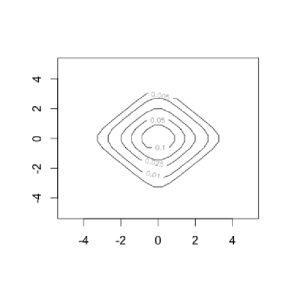
Refer to caption Refer to caption Refer to caption
𝚺=diag(1,1)𝚺diag11\mathbf{\Sigma}=\,\mbox{diag}(1,1), 𝜶=(0,0)𝜶superscript00\mbox{\boldmath$\alpha$}=(0,0)^{\prime}, 𝚺=diag(1,1)𝚺diag11\mathbf{\Sigma}=\,\mbox{diag}(1,1), 𝜶=(2,2)𝜶superscript22\mbox{\boldmath$\alpha$}=(2,2)^{\prime}, 𝚺=diag(1,1)𝚺diag11\mathbf{\Sigma}=\,\mbox{diag}(1,1), 𝜶=(0,0)𝜶superscript00\mbox{\boldmath$\alpha$}=(0,0)^{\prime},
𝝎=(1,1)𝝎superscript11\mbox{\boldmath$\omega$}=(1,1)^{\prime}, 𝝀=(0,0)𝝀superscript00\mbox{\boldmath$\lambda$}=(0,0)^{\prime} 𝝎=(1,1)𝝎superscript11\mbox{\boldmath$\omega$}=(1,1)^{\prime}, 𝝀=(0,0)𝝀superscript00\mbox{\boldmath$\lambda$}=(0,0)^{\prime} 𝝎=(3,3)𝝎superscript33\mbox{\boldmath$\omega$}=(3,3)^{\prime}, 𝝀=(0,0)𝝀superscript00\mbox{\boldmath$\lambda$}=(0,0)^{\prime}
Refer to caption Refer to caption Refer to caption
𝚺=diag(2,2),𝜶=(0,0)formulae-sequence𝚺diag22𝜶superscript00\mathbf{\Sigma}=\,\mbox{diag}(2,2),\mbox{\boldmath$\alpha$}=(0,0)^{\prime}, 𝚺=diag(1,1)𝚺diag11\mathbf{\Sigma}=\,\mbox{diag}(1,1) plus off-diagonal 0.50.50.5, 𝚺=diag(1,1),𝜶=(0,0)formulae-sequence𝚺diag11𝜶superscript00\mathbf{\Sigma}=\,\mbox{diag}(1,1),\mbox{\boldmath$\alpha$}=(0,0)^{\prime},
𝝎=(1,1)𝝎superscript11\mbox{\boldmath$\omega$}=(1,1)^{\prime}, 𝝀=(0,0)𝝀superscript00\mbox{\boldmath$\lambda$}=(0,0)^{\prime} 𝜶=(0,0)𝜶superscript00\mbox{\boldmath$\alpha$}=(0,0)^{\prime}, 𝝎=(1,1)𝝎superscript11\mbox{\boldmath$\omega$}=(1,1)^{\prime}, 𝝀=(0,0)𝝀superscript00\mbox{\boldmath$\lambda$}=(0,0)^{\prime} 𝝎=(1,1)𝝎superscript11\mbox{\boldmath$\omega$}=(1,1)^{\prime}, 𝝀=(3,3)𝝀superscript33\mbox{\boldmath$\lambda$}=(3,3)^{\prime}
Refer to caption Refer to caption Refer to caption
𝚺=diag(1,1)𝚺diag11\mathbf{\Sigma}=\,\mbox{diag}(1,1), 𝜶=(2,2)𝜶superscript22\mbox{\boldmath$\alpha$}=(2,2)^{\prime}, 𝚺=diag(1,1)𝚺diag11\mathbf{\Sigma}=\,\mbox{diag}(1,1), 𝜶=(2,2)𝜶superscript22\mbox{\boldmath$\alpha$}=(2,2)^{\prime}, 𝚺=diag(1,1)𝚺diag11\mathbf{\Sigma}=\,\mbox{diag}(1,1) plus off-diagonal 0.50.50.5,
𝝎=(3,3)𝝎superscript33\mbox{\boldmath$\omega$}=(3,3)^{\prime}, 𝝀=(0,0)𝝀superscript00\mbox{\boldmath$\lambda$}=(0,0)^{\prime} 𝝎=(3,3)𝝎superscript33\mbox{\boldmath$\omega$}=(3,3)^{\prime}, 𝝀=(3,3)𝝀superscript33\mbox{\boldmath$\lambda$}=(3,3)^{\prime} 𝜶=(2,2)𝜶superscript22\mbox{\boldmath$\alpha$}=(2,2)^{\prime}, 𝝎=(3,3)𝝎superscript33\mbox{\boldmath$\omega$}=(3,3)^{\prime}, 𝝀=(3,3)𝝀superscript33\mbox{\boldmath$\lambda$}=(3,3)^{\prime}
Figure 5: Bivariate contour plots of the MSGHD density with 𝝁=(0,0)𝝁superscript00\mbox{\boldmath$\mu$}=(0,0)^{\prime} and varying 𝚺𝚺\mathbf{\Sigma}, 𝜶𝜶\alpha, 𝝎𝝎\omega, and 𝝀𝝀\lambda.
Refer to caption Refer to caption Refer to caption
𝚺=diag(1,1)𝚺diag11\mathbf{\Sigma}=\,\mbox{diag}(1,1), 𝜶=(2,2)𝜶superscript22\mbox{\boldmath$\alpha$}=(2,2)^{\prime}, ϖ=1italic-ϖ1\varpi=1 𝚺=diag(1,1)𝚺diag11\mathbf{\Sigma}=\,\mbox{diag}(1,1), 𝜶=(2,2)𝜶superscript22\mbox{\boldmath$\alpha$}=(2,2)^{\prime}, ϖ=0.5italic-ϖ0.5\varpi=0.5 𝚺=diag(1,1)𝚺diag11\mathbf{\Sigma}=\,\mbox{diag}(1,1), 𝜶=(2,2)𝜶superscript22\mbox{\boldmath$\alpha$}=(2,2)^{\prime}, ϖ=0italic-ϖ0\varpi=0
Refer to caption Refer to caption Refer to caption
𝚺=diag(1,1)𝚺diag11\mathbf{\Sigma}=\,\mbox{diag}(1,1) plus off-diagonal 0.80.80.8, 𝚺=diag(1,1)𝚺diag11\mathbf{\Sigma}=\,\mbox{diag}(1,1) plus off-diagonal 0.80.80.8, 𝚺=diag(1,1)𝚺diag11\mathbf{\Sigma}=\,\mbox{diag}(1,1) plus off-diagonal 0.80.80.8,
𝜶=(0,0)𝜶superscript00\mbox{\boldmath$\alpha$}=(0,0)^{\prime}, ϖ=1italic-ϖ1\varpi=1 𝜶=(0,0)𝜶superscript00\mbox{\boldmath$\alpha$}=(0,0)^{\prime}, ϖ=0.5italic-ϖ0.5\varpi=0.5 𝜶=(0,0)𝜶superscript00\mbox{\boldmath$\alpha$}=(0,0)^{\prime}, ϖ=0italic-ϖ0\varpi=0
Refer to caption Refer to caption Refer to caption
𝚺=diag(1,1)𝚺diag11\mathbf{\Sigma}=\,\mbox{diag}(1,1) plus off-diagonal 0.80.80.8, 𝚺=diag(1,1)𝚺diag11\mathbf{\Sigma}=\,\mbox{diag}(1,1) plus off-diagonal 0.80.80.8, 𝚺=diag(1,1)𝚺diag11\mathbf{\Sigma}=\,\mbox{diag}(1,1) plus off-diagonal 0.80.80.8,
𝜶=(2,2)𝜶superscript22\mbox{\boldmath$\alpha$}=(2,2)^{\prime}, ϖ=1italic-ϖ1\varpi=1 𝜶=(2,2)𝜶superscript22\mbox{\boldmath$\alpha$}=(2,2)^{\prime}, ϖ=0.5italic-ϖ0.5\varpi=0.5 𝜶=(2,2)𝜶superscript22\mbox{\boldmath$\alpha$}=(2,2)^{\prime}, ϖ=0italic-ϖ0\varpi=0
Figure 6: Bivariate contour plots of the MCGHD density varying 𝚺𝚺\mathbf{\Sigma}, 𝜶𝜶\alpha, and ϖitalic-ϖ\varpi.