Path-integral simulation of solids

Abstract

The path-integral formulation of the statistical mechanics of quantum many-body systems is described, with the purpose of introducing practical techniques for the simulation of solids. Monte Carlo and molecular dynamics methods for distinguishable quantum particles are presented, with particular attention to the isothermal-isobaric ensemble. Applications of these computational techniques to different types of solids are reviewed, including noble-gas solids (helium and heavier elements), group-IV materials (diamond and elemental semiconductors), and molecular solids (with emphasis on hydrogen and ice). Structural, vibrational, and thermodynamic properties of these materials are discussed. Applications also include point defects in solids (structure and diffusion), as well as nuclear quantum effects in solid surfaces and adsorbates. Different phenomena are discussed, as solid-to-solid and orientational phase transitions, rates of quantum processes, classical-to-quantum crossover, and various finite-temperature anharmonic effects (thermal expansion, isotopic effects, electron-phonon interactions). Nuclear quantum effects are most remarkable in the presence of light atoms, so that especial emphasis is laid on solids containing hydrogen as a constituent element or as an impurity.

I Introduction

Theoretical methods in condensed-matter science can nowadays accurately predict many observable properties of different kinds of materials. A large number of these properties depend on the atom vibrations around their potential minima. The well-known harmonic approximation for lattice vibrations in crystals may predict rather accurately some of their properties, but omits other basic phenomena such as thermal expansion and some isotopic effects, which are due to the anharmonicity of the interatomic interactions. From a theoretical point of view, consideration of realistic interatomic potentials is a difficult subject, since in actual cases one has to deal with quantum many-body systems at finite temperatures.

A variety of theoretical techniques exist to handle these problems in an approximate way, such as mean-field, infinite-dimension, reduced dimensionality, quasi-harmonic, and several kinds of perturbative methods. Another approach to tackle these problems consists in considering simplified models for which exact solutions can be found, and that will hopefully capture the basic physics of the problem. An alternative route is provided by quantum simulations, which in principle can yield ‘numerically exact’ solutions Ceperley and Alder (1986); Marx and Muser (1999). This means that observable quantities can be obtained for a given many-body Hamiltonian without uncontrolled approximations, taking into account statistical error bars and adequate corrections for the finite size of the simulation cells and the discretized steps in the integration of continuous variables. This is the case of path-integral (PI) simulations of many-body systems, which have been increasingly used in recent years, in parallel with the growing power of available computing facilities.

In his original description of the PI approach, Feynman acknowledged that it was a third formulation of non-relativistic quantum theory, mathematically equivalent to the previous ones by Schrödinger and Heisenberg, and therefore it did not contain fundamentally new results Feynman (1948). He stressed, however, the satisfaction of recognizing old things from a new point of view. At that time it was difficult to appreciate that this new perspective of quantum mechanics was suitable for its implementation as a simulation method in a digital computer, in particular in the field of statistical mechanics. Nowadays, the discretized PI expression of the statistical partition function, interpreted as a quantum-classical isomorphism, allows one to apply powerful methods such as Monte Carlo (MC) and molecular dynamics (MD) to quantum statistical mechanics.

The PI simulation of condensed phases experienced a rapid development in the 1980s and 1990s. Some excellent reviews were published at that time. Chandler and Wolynes presented a deep analysis of the isomorphism between quantum many-body theory and classical statistical mechanics Chandler and Wolynes (1981), building upon the previous proposals of using MC calculations for the quantum partition function by Morita Morita (1973) and Baker Balker (1979). Berne and Thirumalai Berne and Thirumalai (1986) discussed the numerical problems associated to the study of time correlation functions by PI simulations. A didactic introduction to PI simulations was presented by Gillan Gillan (1990), who applied quantum transition-state theory (QTST) of activated processes to study the diffusion of H in metals. Ceperley’s review is an outstanding introduction to path integrals with a focus on the MC techniques required to study collective effects in boson systems such as condensed ⁴He Ceperley (1995). Also Chakravarty’s review of the MC and MD techniques for systems of distinguishable particles, bosons and fermions offers an insightful introduction to PI simulation techniques Chakravarty (1997). Quantum algorithms based on MD methods have been extensively treated by Tuckerman and Hughes Tuckerman and Hughes (1998). In addition to the mentioned reviews, Feynman’s books Feynman and Hibbs (1965); Feynman (1972) contain the grounds of his PI formalism, and remain as a source of basic knowledge for present-day students and researchers. More recently, the extensive monograph by Kleinert Kleinert (1990) addressed the application of path integrals to several scientific areas, while a book by Tuckerman has focused on both PI algorithms and applications in statistical mechanics Tuckerman (2010).

For condensed-matter systems, ab-initio electronic-structure calculations based on density-functional theory (DFT) currently provide good approximations to the total energy and stable atomic configurations. These methods, however, usually treat atomic nuclei as classical particles, and typical quantum effects like zero-point motion are not directly accessible. These effects can be taken into account by approaches such as the quasi-harmonic approximation (QHA), but are difficult to include accurately when large anharmonicities are present, as may happen for light atoms like hydrogen. Thus, to consider the quantum nature of atomic nuclei in condensed-matter systems, path-integral simulations (MC or MD) have proved to be well-suited. A significant advantage of this method is that nuclear degrees of freedom can be quantized in an efficient way, thus allowing to include quantum and thermal fluctuations in many-body systems at finite temperatures. In this manner, MC or MD sampling applied to evaluate finite-temperature path integrals are very useful for performing quantitative and nonperturbative calculations of anharmonic effects in condensed matter Gillan (1988); Ceperley (1995); Marx and Hutter (2009).

For a given solid, quantum effects related to the atomic vibrational motion are relevant at temperatures lower than the Debye temperature of the material, $\Theta_{D}$. At $T\lesssim\Theta_{D}$ the vibrational amplitudes differ from the classical expectancy, so that anharmonic effects on the properties of the material are enhanced with respect to a classical calculation. This includes structural, thermodynamic, and also electronic properties. For example, the low-temperature ($T\to 0$) crystal volume of a (quantum) solid is usually larger than that giving the minimum potential energy in a classical calculation (zero-point expansion). Moreover, the coexistence lines in phase diagrams of different substances are known to be displaced by quantum nuclear motion, as has been revealed by their dependence on isotopic mass. Also, the electronic gap in semiconductors has been found to be renormalized due to nuclear quantum effects on the electron-phonon interaction. For properties that depend on a particular vibrational mode with frequency $\omega$ (e.g., optical or acoustic modes), quantum effects are expected to be relevant at temperatures $T\lesssim\hbar\,\omega/k_{B}$.

A typical quantum effect is the isotopic dependence of several properties of a crystal, which do not vary with the atomic masses in a classical approach. Thus, it is well known that the actual molar volumes of chemically identical crystals with different isotopic composition are not equal, as a consequence of the dependence of the atomic vibrational amplitudes on the atomic mass Buschert et al. (1988); Holloway et al. (1991); Noya et al. (1997a). Lighter isotopes have larger vibrational amplitudes (as expected in a harmonic approximation) and in general they display larger molar volumes as a consequence of anharmonicity. (There are important exceptions to this trend, as happens for systems including hydrogen bonds; see below.) This effect is most noticeable at low temperatures, since the atoms in a solid feel the anharmonicity of the interatomic potential due to zero-point motion. At higher temperatures, the vibrational amplitudes are larger, but the isotope effect on the crystal volume is less prominent, because those amplitudes become less mass-dependent. In the high-temperature (classical) limit this isotope effect disappears. Path-integral simulations have turned out to be sensitive enough to quantify the dependence of crystal volume on the isotopic mass of the constituent atoms Noya et al. (1997a); Herrero (1999); Herrero et al. (2009).

In this topical review we present an introduction to MC and MD algorithms used in PI simulations of condensed-matter systems, i.e., the so-called path-integral Monte Carlo (PIMC) and path-integral molecular dynamics (PIMD). We restrict ourselves to the formalism where quantum effects related to atomic indistinguishability can be neglected. Nuclear exchange effects become important when the de Broglie wavelength, $\lambda=h/\sqrt{2\pi mk_{B}T}$, is comparable to or larger than the average distance between atoms in a solid ($m$: nuclear mass). This is not the case for most of the solids and temperatures studied here, and therefore the PI implementation of exchange for bosonic and fermionic degrees of freedom is not considered. The PI simulation of time dependent correlation functions is another aspect that is not discussed in this review (see Refs. Berne (1986); Hone et al. (2006); Pérez et al. (2009); Habershon et al. (2013)). We summarize the computational requirements to simulate solids in the isothermal-isobaric ($NPT$) ensemble, either using PIMC or PIMD sampling ($N$ stands for the number of particles, while $P$ and $T$ denote pressure and temperature, respectively). We do not present an exhaustive description of existing alternative algorithms for performing PI simulations, rather we prefer to present a minimum of technical information relevant to understand the machinery of a PI computer code, following our own experience in this subject.

In the context of PIMC simulations, there has been a large amount of work for lattice models with the so-called ‘world-line’ method. Applications of this procedure have been from lattice gauge theory of particle physics to models of high-temperature superconductors. Here we will discuss only continuum models, as the techniques employed for lattice models, although related in principle, turn out to be in practice rather different Hirsch et al. (1982); De Raedt and Lagendijk (1985); Von Der Linden (1992); Batrouni and Scalettar (1992). Other quantum simulation methods, such as variational, diffusion, and continuous-time quantum MC, have been employed for the simulation of condensed-matter systems and were reviewed elsewhere Foulkes et al. (2001); Needs et al. (2010); Gull et al. (2011).

The review is organized as follows. In Sec. II, we describe the theoretical background necessary for the implementation of PI simulations of solids. Especial emphasis is laid upon the formulation of the discretization procedure for path integrals at finite temperatures, and its application to calculate average observable quantities in the isothermal-isobaric ensemble. In the remainder of the review we concentrate on the application of these computational methods to different types of solids: noble-gas solids (Sect. III), group-IV materials (Sect. IV), and molecular solids (mainly hydrogen and ice; Sect. V). In Sect. VI we present simulations of the structure and diffusion of point defects in materials, and in Sect. VII we concentrate on nuclear quantum effects in solid surfaces and adsorbates. The review closes with a summary in Sect. VIII.

II Theory

In this section, the definition of the partition function in the $NPT$ ensemble is presented. Then, the discrete PI representation of the partition function is derived for a one-particle ensemble, explaining the suggestive quantum-classical isomorphism. After dealing with the many-body generalization, we summarize the basic algorithms required for both PIMC and PIMD simulations. We comment also on comparative advantages and drawbacks of both methods. Some technical points are illustrated by PI simulations of solid neon in the $NPT$ ensemble. Moreover, we explain the application of PI techniques to calculate rate constants by QTST, vibrational frequencies of solids by a linear-response approach, and free energies by thermodynamic integration.

II.1 Isothermal-isobaric partition function

We focus on the quantum $NPT$ simulation of a solid composed of atoms enclosed in a cell with volume $V$ and periodic boundary conditions. The partition function in the $NPT$ ensemble is given by

$$\triangle(N,P,T)=\intop_{0}^{\infty}dVe^{-\beta PV}Z(N,V,T)\;,$$ (1)

where $\beta$ is the inverse temperature $\beta^{-1}=k_{B}T$ and $k_{B}$ is the Boltzmann constant. The canonical partition function is defined as

$$Z(N,V,T)=\mathrm{Tr}\left[e^{-\beta\widehat{H}}\right]=\sum_{k}e^{-\beta E_{k}}.$$ (2)

$\widehat{H}$ is the Hamiltonian operator, which represents the sum of kinetic ($\widehat{K}$) and potential ($\widehat{U}$) energy terms. $e^{-\beta\widehat{H}}$ is the canonical density operator. This exponential operator is diagonal in the basis of Hamiltonian eigenfunctions. Its trace, $Z$, is the sum, for the complete set of energy eigenfunctions, of the Boltzmann factor associated to each energy eigenvalue, $E_{k}$.

II.2 Path-integral discretization

For didactic purposes, the discretization of the density operator for a free particle is presented in Appendix A. Specifically it is shown that the temperature dependence of the density operator may be approximated by following three steps: an exact factorization of the exponential operator, a formulation of a high-temperature approximation (HTA), and a repeating loop calculation. Here these steps are applied to a general case. For simplicity we consider first the canonical partition function of an ensemble of only one particle with mass $m$ moving in an external potential $U(\mathbf{R})$, $\mathbf{R}$ being a position vector. Let us denote a position eigenfunction as the ket $|\mathrm{\mathbf{R}}_{1}\rangle$. The trace of the density operator over this complete basis set is

$$Z=\int d\mathbf{R}_{1}\,\langle\mathbf{R}_{1}|e^{-\beta\widehat{H}}|\mathbf{R}_{1}\rangle\;.$$ (3)

The temperature dependence of the partition function can be approximated by considering first the exact factorization

$$e^{-\beta\widehat{H}}=\left(e^{-\beta\widehat{H}/L}\right)^{L}\;,$$ (4)

and formulating a convenient HTA for the operator $e^{-\beta\widehat{H}/L}$. A computationally feasible HTA is the Trotter or primitive approximation Schulman (1981)

$$e^{-\beta\widehat{H}/L}\approx e^{-\beta\widehat{U}/2L}\,e^{-\beta\widehat{K}/L}\,e^{-\beta\widehat{U}/2L}\;.$$ (5)

The error of the HTA becomes vanishingly small as $\beta/L\rightarrow 0$, i.e., for Trotter number $L\rightarrow\infty$. We refer to the literature for improved approximations as higher order expansions Takahashi and Imada (1984), cumulant expansions, or pair-product approximations Ceperley (1995). Let us apply the primitive HTA in Eq. (5) to the initial state vector $|\mathbf{R}_{1}\rangle$. Note that $|\mathbf{R}_{1}\rangle$ is an eigenstate of $\widehat{U},$

$$\widehat{U}|\mathbf{R}_{1}\rangle=U(\mathbf{R}_{1})\,|\mathbf{R}_{1}\rangle\;,$$ (6)

but not of $\widehat{H}$. Therefore, the effect of $e^{-\beta\widehat{H}/L}$ on $|\mathbf{R}_{1}\rangle$ will be to project the state $|\mathbf{R}_{1}\rangle$ into a set of different position eigenvectors. One has

$$e^{-\beta\widehat{H}/L}\,|\mathbf{R}_{1}\rangle\approx e^{-\beta\widehat{U}/2L}\,e^{-\beta\widehat{K}/L}\,|\mathbf{R}_{1}\rangle\,e^{-\beta U(\mathbf{R}_{1})/2L}\;.$$ (7)

By inserting the resolution of the identity in momentum space

$$\widehat{I}=\intop d\mathbf{P}\>|\mathbf{P}\rangle\langle\mathbf{P}|\;,$$ (8)

and with the eigenvalue equation

$$\widehat{K}\,|\mathbf{P}\rangle=\frac{P^{2}}{2m}\,|\mathbf{P}\rangle\;,$$ (9)

one gets

$$e^{-\beta\widehat{H}/L}\,|\mathbf{R}_{1}\rangle\approx\\ \int d\mathbf{P}\,e^{-\beta\widehat{U}/2L}\,|\mathbf{P}\rangle\,e^{-\beta P^{2}/2Lm}\,\langle\mathbf{P}|\mathbf{R}_{1}\rangle\,e^{-\beta U(\mathbf{R}_{1})/2L}\;.$$ (10)

Now, by inserting a second resolution of the identity, this time in real space

$$\widehat{I}=\intop d\mathbf{R}_{2}\>|\mathbf{R}_{2}\rangle\langle\mathbf{R}_{2}|\;,$$ (11)

one obtains

$$e^{-\beta\widehat{H}/L}|\,\mathbf{R}_{1}\rangle\approx\int d\mathbf{R}_{2}\,e^{-\beta\left[U(\mathbf{R}_{2})+U(\mathbf{R}_{1})\right]/2L}\,|\mathbf{R}_{2}\rangle\int d\mathbf{P}\,\langle\mathbf{R}_{2}|\mathbf{P}\rangle\,e^{-\beta P^{2}/2Lm}\,\langle\mathbf{P}|\mathbf{R}_{1}\rangle\;.$$ (12)

We recall that the momentum representation of a position function is

$$\langle\mathbf{P}|\mathbf{R}\rangle=\left(\frac{1}{2\pi\hbar}\right)^{3/2}e^{i\mathbf{P\cdot R}/\hbar}\;,$$ (13)

where $\mathbf{P}\cdot\mathbf{R}$ is the scalar product. By substitution of this expression and its complex conjugate, $\langle\mathbf{R}|\mathbf{P}\rangle,$ into Eq. (12) one gets

$$e^{-\beta\widehat{H}/L}|\,\mathbf{R}_{1}\rangle\approx\left(\frac{1}{2\pi\hbar}\right)^{3}\int d\mathbf{R}_{2}\,e^{-\beta\left[U(\mathbf{R}_{2})+U(\mathbf{R}_{1})\right]/2L}\,|\mathbf{R}_{2}\rangle\int d\mathbf{P}\,e^{-\beta P^{2}/2Lm}\,e^{i\mathbf{P}\cdot(\mathbf{R}_{1}-\mathbf{R}_{2})/\hbar}\;.$$ (14)

The momentum integral is Gaussian, so that it can be done analytically with the result

$$e^{-\beta\widehat{H}/L}|\mathbf{R}_{1}\rangle\approx\left(\frac{mL}{2\pi\beta\hbar\text{\texttwosuperior}}\right)^{3/2}\int d\mathbf{R}_{2}\,\exp\left\{-\beta\left[\frac{mL}{2\beta^{2}\hbar^{2}}\left(\mathbf{R}_{1}-\mathbf{R}_{2}\right)^{2}+\frac{U(\mathbf{R}_{2})+U(\mathbf{R}_{1})}{2L}\right]\right\}|\mathbf{R}_{2}\rangle\;.$$ (15)

This approximation for the effect of the exponential operator on $|\mathbf{R}_{1}\rangle$ has a clear physical meaning. It translates this state into a superposition of different positions $|\mathbf{R}_{2}\rangle$ that extend over the whole space. The weight of the new state $|\mathbf{R}_{2}\rangle$ is a positive real number (that one with exponential notation in the integrand) that depends on both the squared distance $\left(\mathbf{R}_{1}-\mathbf{R}_{2}\right)^{2}$ and the potential energy at the positions $\mathbf{R}_{1}$ and $\mathbf{R}_{2}$. Note that the term depending on $\left(\mathbf{R}_{1}-\mathbf{R}_{2}\right)^{2}$ results from the kinetic energy operator of the quantum Hamiltonian.

Having the result of Eq. (15) for the application of $e^{-\beta\widehat{H}/L}$ to the state $|\mathbf{R}_{1}\rangle$, the effect of a new factor $e^{-\beta\widehat{H}/L}$ is a straightforward repeating loop. This operator will project the state $|\mathbf{R}_{2}\rangle$ onto a new position $|\mathbf{R}_{3}\rangle$ with identical weights to those given in Eq. (15), up to a trivial relabeling of the subindex of the position eigenvectors. Note that the weight of the state $|\mathbf{R}_{3}\rangle$ will be the product of the weights associated to the transitions $|\mathbf{R}_{1}\rangle\rightarrow|\mathbf{R}_{2}\rangle$ and $|\mathbf{R}_{2}\rangle\rightarrow|\mathbf{R}_{3}\rangle$, integrated over all $|\mathbf{R}_{2}\rangle$ positions. Successive applications of the exponential operator $e^{-\beta\widehat{H}/L}$ will end after $L$ steps with the state $|\mathbf{R}_{L+1}\rangle$. The weight of $|\mathbf{R}_{L+1}\rangle$ is then the product of the $L$ weights associated to each step in the chain of transitions $|\mathbf{R}_{1}\rangle\rightarrow|\mathbf{R}_{2}\rangle\ldots\rightarrow|\mathbf{R}_{L+1}\rangle$, integrated over all intermediate positions.

To obtain the partition function of Eq. (3), the last operation is to perform the dot product with the bra $\langle\mathbf{R}_{1}|$ and to integrate over $\mathbf{R}_{1}.$ The orthogonality of the position eigenstates implies that

$$\langle\mathbf{R}_{1}|\mathbf{R}_{L+1}\rangle=\delta(\mathbf{R}_{1}-\mathbf{R}_{L+1})\;,$$ (16)

where $\delta$ denotes the Dirac delta function. Thus the final state $|\mathbf{R}_{L+1}\rangle$ is restricted to be identical to the initial state $|\mathbf{R}_{1}\rangle$. With this condition, i.e., $\mathbf{R}_{L+1}=\mathbf{R}_{1}$, the discretized approximation of $Z$ is

$$Z\approx\left(\frac{mL}{2\pi\beta\hbar^{2}}\right)^{\frac{3L}{2}}\int d\mathbf{R}_{1}\ldots d\mathbf{R}_{L}\,\exp\left\{-\beta\sum_{i=1}^{L}\left[\frac{mL}{2\beta^{2}\hbar^{2}}\left(\mathbf{R}_{i}-\mathbf{R}_{i+1}\right)^{2}+\frac{U(\mathbf{R}_{i})}{L}\right]\right\}_{\mathbf{R}_{L+1}=\mathbf{R}_{1}}\;.$$ (17)

There are several points to stress. The first one is that the limit $L\rightarrow\infty$ of this expression converges to the exact path-integral formulation of $Z$. We refer to the literature for those readers interested in the continuum limit of this expression Feynman (1972); Kleinert (1990); Tuckerman (2010). Quantum PI simulations rely on the use of a discretized form such as the one in Eq. (17). A second aspect is that Eq. (17) is formally equivalent to the partition function of a classical ring-polymer composed of $L$ beads or replicas $(\mathbf{R}_{1},\mathbf{R}_{2},\ldots,\mathbf{R}_{L})$ of the same quantum particle. The ring-polymer interacts through an effective potential given by the sum of two contributions

$$U_{\rm spr}=\left\{\sum_{i=1}^{L}\frac{mL}{2\beta^{2}\hbar^{2}}\left(\mathbf{R}_{i}-\mathbf{R}_{i+1}\right)^{2}\right\}_{\mathbf{R}_{L+1}=\mathbf{R}_{1}}\;,$$ (18)

$$U_{\rm int}=\sum_{i=1}^{L}\frac{U(\mathbf{R}_{i})}{L}\;.$$ (19)

The first term, $U_{\rm spr}$, represents a harmonic interaction between neighboring beads at $\mathbf{R}_{i}$ and $\mathbf{R}_{i+1}$. The coupling constant increases along with the number of beads, the particle mass and the squared temperature. The second term, $U_{\rm int}$, is the total potential energy of the beads with the true Hamiltonian scaled by a factor $1/L$ (i.e., it corresponds to the mean potential energy for the true Hamiltonian).

This suggestive result is the so-called quantum-classical isomorphism. It establishes that the quantum partition function can be approximated with arbitrary accuracy by means of a classical system interacting through the effective potential

$$U_{\rm eff}=U_{\rm spr}+U_{\rm int}\;.$$ (20)

A particularity of the classical isomorph, when compared to a real classical system, is that its potential energy $U_{\rm spr}$ depends explicitly on both the temperature and particle mass. The classical limit for the potential $U(\mathbf{R})$ is easily achieved within the discretized PI algorithm by setting the Trotter number $L$ = 1, so that $U_{\rm spr}\equiv 0$ and $U_{\rm int}\equiv U$.

II.3 Many-body extension

The generalization of the previous one-particle results is straightforward for the case that identical quantum particles are treated by Boltzmann statistics. The position vectors need now a second index to label each particle. Thus $\mathbf{R}_{ij}$ denotes the position vector associated to the $i^{\prime}$th bead of the $j^{\prime}$th particle. Assuming for simplicity that there are $N$ identical particles with mass $m$, then the harmonic interaction includes a sum over the $N$ particles

$$U_{\rm spr}=\sum_{j=1}^{N}\left\{\sum_{i=1}^{L}\frac{mL}{2\beta^{2}\hbar^{2}}\left(\mathbf{R}_{ij}-\mathbf{R}_{(i+1)j}\right)^{2}\right\}_{\mathbf{R}_{(L+1)j}=\mathbf{R}_{1j}}\;.$$ (21)

The interaction energy term is simply

$$U_{\rm int}=\frac{1}{L}\,\sum_{i=1}^{L}U_{i}\;,$$ (22)

where $U_{i}$ is the potential energy associated to the $i$’th replica of the system, composed of $N$ classical particles at $(\mathbf{R}_{i1},\mathbf{R}_{i2},\ldots,\mathbf{R}_{iN})$:

$$U_{i}\equiv U\left(\mathbf{R}_{i1},\mathbf{R}_{i2},\ldots,\mathbf{R}_{iN}\right)\;.$$ (23)

$U_{\rm int}$ is then the average potential energy over the $L$ replicas of the system.

The canonical partition function is approximated as

$$Z(NVT)\approx\\ \frac{1}{N!}\left(\frac{mL}{2\pi\beta\hbar\text{\texttwosuperior}}\right)^{3NL/2}\int d\Gamma\exp\left[-\beta\left(U_{\rm spr}+U_{\rm int}\right)\right]\;,$$ (24)

where $d\Gamma=\prod_{j=1}^{N}\prod_{i=1}^{L}d\mathbf{R}_{ij}$, and the particle indistinguishability has been considered by the $N!$ term. The thermal behavior of the quantum system can be explored by applying conventional MC or MD simulation techniques on the classical ring-polymer isomorph.

For a series of PI simulations of the same model at different temperatures, it is sensible to use the same value of $\epsilon$ in the HTA of Eq. (7), so that

$$\epsilon=\frac{\beta}{L}=\frac{1}{k_{B}TL}$$ (25)

remains independent of $T$. This condition implies that $L$ should be varied as $T^{-1}$. Thus, the number of beads, $L$, as well as the computational cost of the simulations, increases as the temperature lowers. In general, different thermodynamic properties may display different convergence with the Trotter number $L$ Ceperley (1995). An empirical rule to estimate a reasonable value of $TL$ is the following. For a solid where the largest vibrational frequency of its phonon spectrum is $\omega_{max}$ one should take

$$\epsilon^{-1}=k_{B}TL\geq 4\hbar\,\omega_{max}\;.$$ (26)

In words this means that the thermal energy corresponding to the temperature $TL$ of the HTA must be at least about four times larger than the energy quantum of the system under consideration.

II.4 Path-integral Monte Carlo

For simplicity we consider here a rigid simulation cell, so that volume fluctuations in the $NPT$ ensemble are restricted to be isotropic. The general case of a flexible simulation cell can be treated by techniques that were originally introduced for MD simulations, but can be also applied to MC methods Parrinello and Rahman (1980, 1981); Souza and Martins (1997). In a possible setup of the PIMC method in the isothermal-isobaric ensemble, the coordinates $\mathbf{R}_{ij}$ are updated according to three different types of sampling schemes.

The first one consists of trial moves of the individual coordinates $\mathbf{R}_{ij}$. The trials may be performed sequentially for every bead coordinate $i$ and every atom $j$. The trial configuration is accepted with probability

$$P_{\rm acc}=\mathrm{min\left[1,\exp\left(-\beta\triangle\mathit{U_{\rm eff}}\right)\right]}\;,$$ (27)

where $\triangle U_{\rm eff}$ is the difference of $U_{\rm eff}$ between the new and old configurations.

The second type of sampling corresponds to trial moves of the center of mass (centroid) of the ring-polymers

$$\mathbf{X}_{j}=\frac{1}{L}\sum_{i=1}^{L}\mathbf{R}_{ij}\;,$$ (28)

which are performed sequentially for every atom $j$ of the simulation cell. This type of move maintains unaltered the shape of the individual ring-polymers. This move is essential to explore efficiently the configurational space, specially at temperatures where thermal fluctuations are significant for the spatial atomic delocalization Berne and Thirumalai (1986). The acceptance criterion is the same as in Eq. (27), although for this type of move the harmonic interaction, $U_{\rm spr}$, remains unaltered and needs not be recalculated.

The third type of sampling consists of trial changes in the volume of the simulation cell. The volume change ($V\rightarrow V_{new}$) implies that all particle coordinates change accordingly, so that they are scaled by $s=(V_{new}/V)^{1/3}$. The acceptance probability of the trial configuration is Frenkel and Smit (1996)

$$P_{\rm acc}=\\ \mathrm{min}\left\{1,\exp\left(-\beta\left[\triangle\mathit{U_{\rm eff}}+\mathit{P\,\triangle V-k_{B}TNL\ln}\frac{V_{new}}{V}\right]\right)\right\}\;.$$ (29)

For given $T$ and $P$ the maximum change allowed for random moves of the bead coordinates ($\mathbf{R}_{ij}$), ring-polymer centroids ($\mathbf{X}_{j}$), and volume is typically adjusted to yield an acceptance ratio of attempted moves of about 50% for each kind of sampling.

Alternative methods for PIMC simulations are formulated based on the Fourier representation of the ring-polymer configurations Freeman and Doll (1984); Coalson (1986); Chakravarty et al. (1998), and also on combined schemes using both real and Fourier space representations of ring-polymers Vorontsov-Velyaminov et al. (1997).

The trajectory generated by the MC algorithm is made of a set of configurations, each one defined by the volume and the bead positions $\left(V,\left\{\mathbf{R}_{ij}\right\}\right)$. For each configuration it is straightforward the estimation of several important observables, as the kinetic energy, internal energy, and pressure. The expression of these estimators in either $NPT$ or $NVT$ ensembles is the same. The average kinetic energy, $\langle K\rangle$, is derived from the thermodynamic relation

$$\langle K\rangle=\frac{m}{\beta}\,\frac{\partial\ln Z}{\partial m}\;.$$ (30)

Applying this expression to Eq. (17) results on the primitive estimator of the kinetic energy

$$K_{p}=\frac{3NL}{2\beta}-U_{\rm spr}\;,$$ (31)

where the $U_{\rm spr}$ is calculated with Eq. (21). Note that we have written the result in terms of $K_{p}$ instead of $\left\langle K_{p}\right\rangle$, since the former refers to the kinetic energy estimator of a single configuration $\left(V,\left\{\mathbf{R}_{ij}\right\}\right)$, while the latter denotes the ensemble average, i.e., an average over the whole MC trajectory. The virial estimator of the kinetic energy is physically equivalent, but it displays an improved numerical convergence Herman et al. (1982); Parrinello and Rahman (1984)

$$K_{v}=\frac{3N}{2\beta}+\frac{1}{2L}\sum_{j=1}^{N}\sum_{i=1}^{L}\left(\mathbf{R}_{ij}-\mathbf{X}_{j}\right)\cdot\nabla_{\mathbf{R}_{ij}}U_{i}\;,$$ (32)

where $-\nabla_{\mathbf{R}_{ij}}U_{i}$ is the force on the bead located at $\mathbf{R}_{ij}$, i.e., the force on the atom $j$ of the $i$’th replica of system, as derived from the potential function $U(\mathbf{R}_{i1},\mathbf{R}_{i2},\ldots,\mathbf{R}_{iN})$ in Eq. (23). The position vector $\mathbf{X}_{j}$ is the centroid of the atom $j$ [see Eq. (28)]. Note that while the virial estimator requires the calculation of the atomic forces at all bead positions, the primitive estimator needs only to know the harmonic energy $U_{\rm spr}$. The estimator of the internal energy is derived analogously from

$$\langle E\rangle=-\frac{\partial\ln Z}{\partial\beta}$$ (33)

as

$$E=K_{v}+U_{\rm int}\;,$$ (34)

where $U_{\rm int}$ is given in Eq. (22).

The pressure estimator is derived from

$$\left\langle\mathcal{P}\right\rangle=\frac{1}{\beta}\,\frac{\partial\ln Z}{\partial V}$$ (35)

with the result

$${\cal P}=\frac{NL}{\beta V}-\frac{2}{3V}U_{\rm spr}-\frac{1}{L}\sum_{i=1}^{L}\frac{\partial U_{i}}{\partial V}\,.$$ (36)

The volume derivative can be calculated either analytically or numerically by considering that an increase of the actual volume by $\triangle V$ will change each bead coordinate of the simulation cell by a scaling factor $s=(1+\Delta V/V)^{1/3}$.

A final important relation for the isothermal compressibility $\kappa_{T}$, valid in the $NPT$ ensemble, is the following:

$$\kappa_{T}=-\frac{1}{\langle V\rangle}\,\frac{\partial\langle V\rangle}{\partial P}=\frac{\beta\,\sigma_{V}^{2}}{\langle V\rangle}\;,$$ (37)

where the volume fluctuations are

$$\sigma_{V}^{2}=\langle V^{2}\rangle-\langle V\rangle^{2}\;.$$ (38)

A deep analysis on the derivation of compressibilities from PI simulations was presented by Sesé Sesé (2003).

II.5 Path-integral molecular dynamics

First of all, it is important to make clear that the dynamics considered in the PIMD method is artificial. It is suitable for efficiently sampling the partition function in Eq. (24) and thus for evaluating static or equilibrium properties, but it does not represent the real quantum dynamics of the systems under investigation.

An efficient implementation of classical dynamics to sample the microstates associated to the discretized partition function in Eq. (24) requires the use of numerical techniques adapted to this problem. The potential term in Eq. (21) implies that we have a cyclic chain of coupled harmonic oscillators giving rise to a wide spectrum of different vibrational frequencies. Integration of the dynamic equations is numerically more stable if all modes oscillated in the same time scale. Besides, if the number of beads $L$ increases, then for a given replica the harmonic coupling constant in Eq. (21) becomes larger while the effective interaction potential on each bead becomes smaller, because of the factor $L^{-1}$ in Eq. (22). Dominance of harmonic forces makes that ergodicity problems can be present in the classical bead dynamics.

The set-up of effective algorithms to perform PIMD simulations has been described in detail by Martyna et al. Martyna et al. (1996, 1999) and by Tuckerman Tuckerman (2002, 2010). The main steps of a possible implementation are based on the use of: $i)$ staging variables to bring harmonic modes to the same time scale; $ii)$ massive thermostatting techniques to avoid ergodicity problems; $iii)$ reversible integrators and multiple time steps to integrate the classical equations of motion by a factorization of the classical Liouville operator. A detailed account of these algorithms is outside the scope of the present review so that we limit ourselves to present a brief overview of this PIMD implementation.

Staging bead coordinates $u_{ij}$ are defined by a linear transformation that diagonalizes the harmonic energy in Eq. (21) Tuckerman and Hughes (1998); Tuckerman (2002). For a given atom $j$ the staging mode coordinates are defined as

$$\mathbf{u}_{1j}=\mathbf{R}_{1j}\;,$$ (39)

$$\mathbf{u}_{ij}=\mathbf{R}_{ij}-\frac{i-1}{i}\,\mathbf{R}_{(i+1)j}-\frac{1}{i}\,\mathbf{R}_{1j}\;,\;i=2,\dots,L\;.$$ (40)

The masses of the staging modes are defined as

$$m_{1}=0,$$ (41)

$$m_{i}=\frac{i}{i-1}\,m\;,\;i=2,\dots,L\;,$$ (42)

where $m$ is the mass of atom $j$. The harmonic term in Eq. (21) is transformed to a diagonal form with the staging coordinates:

$$U_{\rm spr}=\sum_{j=1}^{N}\sum_{i=2}^{L}\frac{m_{i}L}{2\beta\text{\texttwosuperior}\hbar^{2}}\,\mathbf{u}_{ij}^{2}\;.$$ (43)

Momentum variables for the MD algorithm are introduced through the substitution of the prefactor in the partition function in Eq. (24) by a Gaussian integral over momentum coordinates

$$\left(\frac{mL}{2\pi\beta\hbar^{2}}\right)^{3NL/2}=C\int\prod_{j=1}^{N}\prod_{i=1}^{L}d\mathbf{P}_{ij}\exp\left(-\frac{\beta\,\mathbf{P}_{ij}^{2}}{2\,m_{i}^{\prime}}\right)\;.$$ (44)

$\mathbf{P}_{ij}$ is the momentum associated to the $i$’th staging mode of the $j$’th particle, while $C$ is a constant that depends on the masses and has no influence in the calculated equilibrium properties. The masses $m_{i}^{\prime}$ are chosen so that the staging modes with $i=2,\ldots L$ move on the same time scale

$$m^{\prime}_{1}=m\;,$$ (45)

$$m^{\prime}_{i}=m_{i},\;\mathrm{f\mathrm{or}}\;i=2,\ldots,L\;.$$ (46)

With this extension, the sampling of the partition function in Eq. (24) is made now by a classical MD algorithm in the phase space expanded by the set of coordinates $\left\{\mathbf{u}_{ij},\mathbf{P}_{ij}\right\}$. An additional advantage of the staging modes is that both the transformation $\left\{\mathbf{u}_{ij}\right\}\rightarrow\left\{\mathbf{R}_{ij}\right\}$ and its inverse are easily done by simple recursion relations Tuckerman et al. (1993). An alternative to the staging variables is based on the normal mode transformation of the bead coordinates Tuckerman and Hughes (1998).

The temperature control in either the $NVT$ or $NPT$ ensembles is achieved by a massive thermostatting of the system that implies a chain of Nosé-Hoover thermostats coupled to each of the staging variables $\mathbf{u}_{ij}$ Martyna and Klein (1992); Tuckerman and Hughes (1998). The thermostat ‘mass’ parameter, $Q$, is set to evolve in the scale of the harmonic bead forces as Tuckerman and Hughes (1998)

$$Q=\frac{\beta\,\hbar^{2}}{L}\;.$$ (47)

In the case of the $NPT$ ensemble, the volume itself is a dynamic variable coupled to a chain of barostats in order to maintain a constant pressure. The volume and barostat ‘mass’ parameters are set as Martyna et al. (1999)

$$W=\frac{3\,(NL+1)}{\beta\,\omega_{b}^{2}}\;,$$ (48)

$$Q_{p}=\frac{1}{\beta\,\omega_{b}^{2}}\;.$$ (49)

The frequency $\omega_{b}$ is taken to be 1 ps^-1.

The dynamic equations in the $NPT$ ensemble are the time derivatives of both position and momentum coordinates of each dynamic degree of freedom of the extended system, i.e., the staging modes, the chains of Nosé-Hoover thermostats, the volume, and the chain of barostats Martyna et al. (1999). The thermostats and barostats introduce friction terms in the dynamic equations, which cause that the extended dynamics is not Hamiltonian. Nevertheless there is a quantity, playing the role of a total energy in the extended system, that is conserved along the time evolution. The conservation of this energy is a useful check for the numerical integration of the equations of motion.

The reversible extended-system multiple time-step integration is well documented in Refs. Martyna et al. (1999); Tuckerman and Hughes (1998); Tuckerman et al. (2006, 1992). The factorization of the classical Liouville propagator, $\exp\left(t\frac{\partial}{\partial t}\right)$, appears at first sight rather complicated, but it is in fact straightforward and relatively easy to implement as a computer code. For this implementation it is advisable to start programming the factorization of the exponential propagator in the microcanonical $NVE$ ensemble, as both thermostat and barostat variables are absent. Having a checked $NVE$ integrator, one can extend the algorithm to the $NVT$ ensemble, which implies to add the somewhat lengthy factorization associated to the integration of the Nosé-Hoover chains. The next step would be to include both volume and the chain of barostats as dynamic variables to allow for $NPT$ simulations. The last step of this build-up would be to allow for the full flexibility in the simulation cell of the $NPT$ ensemble Martyna et al. (1999).

The estimators in the PIMD method are similar to those presented for PIMC . The only difference is the term associated to the momentum variable. For example, the PIMC pressure estimator shown in Eq. (36) changes to

$${\cal P}=\frac{2}{3V}\sum_{i=1}^{L}\sum_{j=1}^{N}\frac{\mathbf{P}_{ij}^{2}}{2\,m^{\prime}_{i}}-\frac{2}{3V}\,U_{\rm spr}-\frac{1}{L}\sum_{i=1}^{L}\frac{\partial U_{i}}{\partial V}\;.$$ (50)

Note that the equipartition principle implies that the ensemble average of the first term on the right-hand side is

$$\sum_{i=1}^{L}\sum_{j=1}^{N}\left\langle\frac{\mathbf{P}_{ij}^{2}}{2\,m^{\prime}_{i}}\right\rangle=\frac{3NL}{2\,\beta}\;,$$ (51)

so that the PIMC and PIMD pressure estimators in Eqs. (36) and (50) should provide identical expectation values in converged equilibrium simulations.

II.6 PIMC versus PIMD: solid Ne simulations

PIMC is conceptually simpler than PIMD. First, it requires to work in the configurational space expanded by the bead coordinates, while PIMD needs also bead velocities. Second, the algorithm for MC simulation requires to know the potential energy of the system but not the atomic forces, contrary to the PIMD method. And third, the control of external parameters, as the pressure and temperature, is easier in a MC approach. In addition, an efficient treatment of particle exchange (fermionic or bosonic degrees of freedom) is only possible in a MC approach Ceperley (1995).

In spite of the larger simplicity of the PIMC algorithm, the code of a PIMC program may require more effort than that of a PIMD method. The reason is that in a MC sampling one needs to calculate the potential energy change associated to random moves of the system. An efficient code restricts this calculation only to the energy terms affected by the move, avoiding to recalculate those that remain invariant. E.g., for a pairwise potential a random move of a particle requires to calculate the interaction energy of the moving particle with the rest of the system, all other pairwise interactions remain invariant and need not to be recalculated. Thus, an efficient MC implementation can not be done for an arbitrary potential model, but requires the development of a specific computer code for both the particular move type and the model at hand.

Then, the PIMC approach might be a disadvantage if one needs to use different potential models, because it requires usually writing and checking large parts of new computer code. However, such implementation is straightforward in PIMD. Here the update algorithm (integration of the equations of motion of both position and momentum coordinates) is coupled to the potential model only by the transfer of an array with the actual value of the atomic forces. Thus, implementation of a new model is easier as it does not affect the general structure of a PIMD code.

Another important difference between both methods is that a typical MC move implies a sequential updating of each bead coordinate. In contrast, in a MD simulation all bead coordinates are simultaneously updated at each time step. Then, as the number of atoms increases over certain boundary, trajectories generated by PIMD may explore the configuration space much faster than PIMC, which translates into lower requirements of computational resources. Besides, the global updates of the PIMD method, as opposed to PIMC, imply an easier implementation of parallelization strategies in the computer code.

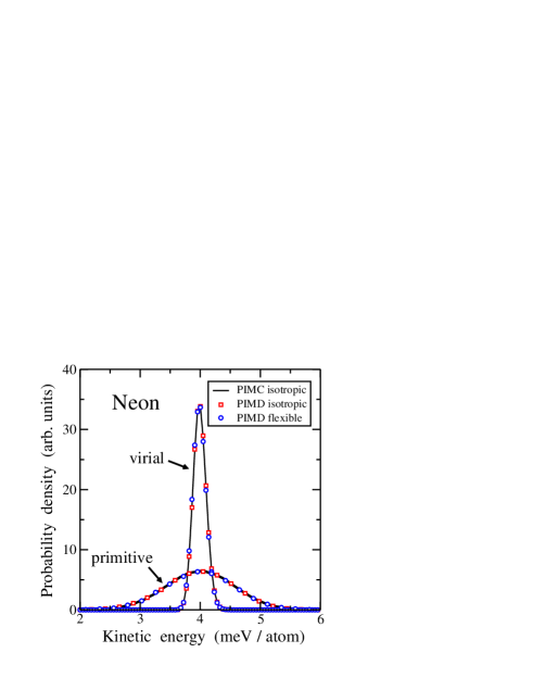
Figure 1: Probability distribution of the kinetic energy per atom for solid neon at $T=20$ K and $P=0$, as derived by primitive and virial estimators. The results correspond to three different $NPT$ simulation methods: PIMC and PIMD with isotropic volume fluctuations, as well as PIMD with full cell flexibility.

To compare results obtained from both methods with a simple interatomic potential, PIMC and PIMD test simulations are presented here for solid Ne. The noble-gas atoms are treated as particles of mass $m=20.18$ amu (mean mass for natural isotopic composition) interacting through a Lennard-Jones 6-12 potential of the form

$$U(r)=4\,\epsilon\left[\left(\frac{\sigma}{r}\right)^{12}-\left(\frac{\sigma}{r}\right)^{6}\right]\;,$$ (52)

with parameters $\epsilon=3.2135$ meV and $\sigma=2.782$ Å. This pair potential is truncated at distances $r$ larger than $r_{c}=2.5\,\sigma$. The simulation cell is a $3\times 3\times 3$ supercell of the standard fcc unit cell, containing $N=108$ atoms subject to periodic boundary conditions. Standard long-range corrections were computed assuming that the pair correlation function is unity for $r>r_{c}$, leading to well-known corrections for the pressure and internal energies Johnson et al. (1993). The number of beads was set by the condition $L\,T=200$ K. A PIMC run consisted of $10^{6}$ MC steps with a previous equilibration of $10^{5}$ steps. Each step included: $i)$ a sequential trial move of each of the $N\times L$ beads; $ii)$ a sequential trial move of each centroid in the $N$ ring-polymers; $iii)$ a trial move of the simulation cell volume.

PIMD simulations were performed with $10^{6}$ MD steps with an equilibration of $10^{5}$ steps. A chain of four Nosé-Hoover thermostats was coupled to each of the staging variables and a chain of four barostats was coupled to the volume. The equations of motion were integrated using a time step of $\triangle t=3$ fs for both the Lennard-Jones and barostat interactions, and a smaller one of $\triangle t/4$ for both the thermostat and harmonic interactions. PIMD simulations in the $NPT$ ensemble were performed by allowing either isotropic volume fluctuations or full cell flexibility. In the latter case the simulation cell was not allowed to rotate in space. With this restriction the number of independent degrees of freedom to describe a fully flexible unit cell is reduced from 9 to 6 cit .

The equivalence between PIMC and PIMD simulations in the $NPT$ ensemble is illustrated by the results on solid Ne. In both simulation methods we allow for isotropic volume fluctuations, and in the case of PIMD we additionally consider simulations with a full flexibility of the simulation cell. In Fig. 1 the distribution function of the kinetic energy of the solid per simulation cell is presented at $T=20$ K and $P=0$, using both the virial and the primitive estimators. For each estimator the results obtained by both PIMC and PIMD methods are shown. Notice that the virial estimator produces a significantly narrower kinetic energy distribution. However, the expected value of the kinetic energy is, within the statistical noise, identical for both estimators. The agreement between PIMC and PIMD simulations, as well as between PIMD data for isotropic volume fluctuations and full cell flexibility, is a strong evidence that the correct ensemble distribution is being explored in the various simulations.

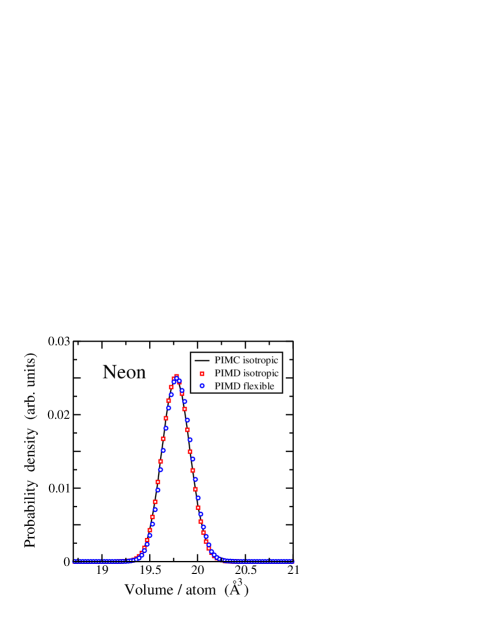
Figure 2: Probability distribution of the volume for the $NPT$ simulation of solid Ne at $T=20$ K and $P=0.2$ GPa. The data were derived by PIMC and PIMD with isotropic volume fluctuations, as well as by PIMD with full cell flexibility.

This conclusion is further supported by the probability density of the volume of solid Ne at $T=20$ K and $P=0.2$ GPa displayed in Fig. 2. An unbiased sampling should provide the expected value of equilibrium properties and also the fluctuations of the thermodynamic properties according to the employed ensemble. We recall that in the $NPT$ ensemble the volume fluctuation has an important physical meaning, as it is related to the compressibility of the solid [see Eq. (37)]. The volume distributions shown in Fig. 2 provide a non-trivial test for the pressure control in the PIMD method. This pressure control is much easier, and less prone to error, using a PIMC algorithm. Thus, the agreement found between the volume sampled by both methods is a necessary condition for the correctness of the employed algorithms. Also relevant is the agreement found in the PIMD simulations using fully flexible and rigid simulation cells. We stress that a pre-requisite for this agreement is to set the correct number of degrees of freedom in the dynamic equation of the barostat coupled to the volume cit .

The equation of state $P$–$V$ of solid Ne at $T=20$ K is presented in Fig. 3 for pressures in the range from 0 to 0.23 GPa. The state points were studied by both PIMC and PIMD simulations, and in the latter case by sampling either isotropic or fully flexible volume fluctuations. Note the good agreement obtained between the three sets of simulations.

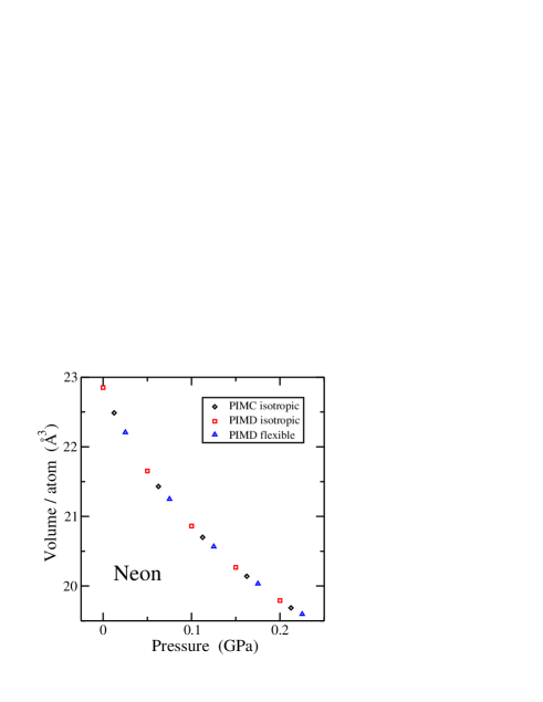
Figure 3: Equation of state $P$–$V$ of solid Ne at 20 K. The data correspond to $NPT$ simulations by three different methods: PIMC and PIMD with isotropic volume fluctuations, as well as PIMD with full cell flexibility.

II.7 Quantum transition-state theory

Classical transition-state theory is a well-established approximation for the calculation of rate constants associated to the kinetics of infrequent events. For the activated diffusion of an impurity in a solid, the key element in this theory is the calculation of a ratio between the probability for finding the impurity at a barrier region ($B$) and at its stable configuration ($S$), where the barrier region must be specified for the given kinetic process. A quantum generalization of classical transition-state theory has been developed based on the PI formulation. According to this approach, the calculation of jump rates depends on the ratio, $P_{c}$, between the probabilities of finding the diffusing particle at the saddle-point and at the stable site. Thus, the jump rate constant is given by

$$k=\frac{1}{2}\,\overline{v}\,\frac{P_{c}}{l}\;,$$ (53)

where $\overline{v}$ is a factor weakly dependent on temperature, taken to be the thermal velocity $\overline{v}=\sqrt{2/(\pi\beta m)}$ of the jumping particle, and $l$ is the jumping distance.

The probability ratio $P_{c}$ is proportional to the Boltzmann factor $\exp(-\beta\triangle F)$, where $\triangle F$ is the free energy barrier for the activated process. Thus, the jump rate (a dynamical quantity) is closely related to the free energy difference $\triangle F$ (a time-independent quantity), so that its temperature dependence can be calculated from equilibrium simulations without any dynamical information.

A direct estimation of the probability $P_{c}$ by a simulation is difficult in the case that the diffusion event is infrequent. A convenient approach to this calculation was first proposed by Gillan Gillan (1987a) as the reversible work done on the system when the centroid of the diffusing particle ($\mathbf{X}_{j}$) moves along the diffusion path $S\rightarrow B$

$$P_{c}=\exp\left(\beta\int_{S}^{B}\mathbf{f}(\mathbf{X}_{j})\,d\mathbf{X}_{j}\right)$$ (54)

where $\mathbf{f}(\mathbf{X}_{j})$ is the mean force acting on the jumping impurity with its centroid fixed on $\mathbf{X}_{j}$

$$\mathbf{f}(\mathbf{X}_{j})=-\left\langle\frac{1}{L}\sum_{i=1}^{L}\nabla_{\mathbf{R}_{ij}}U_{i}\right\rangle_{\mathbf{X}_{j}}$$ (55)

The meaning of $\nabla_{\mathbf{R}_{ij}}U_{i}$ was explained after Eq. (32). The average value in Eq. (55) is taken over a sampling of configurations where the ring-polymer of the jumping impurity is constrained to be fixed at $\mathbf{X}_{j}$. Note that by fixing the centroid of the impurity, we are suppressing its classical spatial delocalization. The integration in Eq. (54) is performed along a path $S\rightarrow B$ typically discretized into about ten equidistant $\mathbf{X}_{j}$ points. Quantum effects that may give rise to substantial deviations from the classical jump rate are taken into account within the QTST. In this way, jump rates for kinetic processes can be readily approximated for realistic, highly nonlinear many-body problems, even at quite low temperatures. Thus, this technique provides a methodology to study the influence of vibrational mode quantization and quantum tunneling on impurity jump rates.

In contrast to the case of equilibrium properties, where PI methods are well established and controllable (at least for distinguishable and bosonic particles), the PI simulation of time-dependent properties still remains as an open numerical problem. Several approximations, such as centroid MD Cao and Voth (1994a, b); Jang and Voth (1999) and ring-polymer MD Craig and Manolopoulos (2004), have been formulated to tackle this problem, but there is at present no widespread consensus on their general reliability. We refer to the recent literature for those readers interested in this topic Pérez et al. (2009); Habershon et al. (2013).

II.8 Linear-response approach for vibrational frequencies

An interesting application of path-integral simulations to solids is the calculation of vibrational frequencies by using the static isothermal susceptibility tensor $\chi^{T}$ Ramírez and Herrero (2005). This tensor gives the linear response (LR) of a system (e.g., solid or molecule) in thermal equilibrium to vanishingly small forces applied on the atomic nuclei. For solids, in particular, this method offers a practical approach to derive phonon energies by a non-perturbative method, and the representation of the response function within the path-integral formulation offers a simple way for its numerical calculation Ramírez and López-Ciudad (2001); López-Ciudad et al. (2003). In fact, $\chi^{T}$ can be readily derived from PI simulations of a solid at equilibrium, without having to explicitly impose any external forces during the simulation. This LR approach is able to realistically reproduce vibrational properties that are strongly affected by anharmonicity, and thus represents a significant improvement as compared to the standard harmonic approximation. A sketch of the method is given in the following.

Let us denote the set of $N$ centroid positions $\left\{\mathbf{X}_{1},\ldots,\mathbf{X}_{N}\right\}$ of the atoms in the simulation cell as a vector with components $X_{j}$ ($j=1,\dots,3N$). See Eq. (28) for the centroid definition. The susceptibility tensor ${\chi}^{T}$, with dimensions $3N\times 3N,$ is defined in terms of the centroid coordinates as Ramírez and López-Ciudad (2001)

$$\chi_{ij}^{T}=\beta\,\sqrt{m_{i}m_{j}}\;\mu_{ij}\;,$$ (56)

where $m_{i}$ is the mass of the atom associated to component $i$, $\mu_{ij}=\langle X_{i}X_{j}\rangle-\langle X_{i}\rangle\langle X_{j}\rangle$ is the covariance of the centroid coordinates $X_{i}$ and $X_{j}$, and $\langle\dots\rangle$ indicates an ensemble average.

The tensor ${\chi}^{T}$ allows us to derive a LR approximation to the excitation energies of the vibrational system, that is applicable even to highly anharmonic situations. The LR approximation for the vibrational frequencies reads

$$\omega_{n,{\rm LR}}=\frac{1}{\sqrt{\Delta_{n}}}\;,$$ (57)

where $\Delta_{n}$ ($n=1,\dots,3N$) are the eigenvalues of $\chi^{T}$, and the LR approximation to the first excitation energy of vibrational mode $n$ is given by $\hbar\,\omega_{n,{\rm LR}}$. More details on the method and illustrations of its ability for predicting vibrational frequencies of solids and molecules can be found elsewhere Ramírez and López-Ciudad (2001, 2002); López-Ciudad et al. (2003); Ramírez and Herrero (2005).

II.9 Free-energy calculation

The simulation of the phase diagram and phase coexistence properties of a given material requires the calculation of its free energy. Thermodynamic integration (TI) is one of the most widely employed methods to compute free energies Kirkwood (1935); Allen and Tildesley (1987); Frenkel and Smit (1996). It is based on the construction of a thermodynamic path defined by making the canonical partition function $Z_{\lambda}$ to depend upon a control parameter $\lambda$ that is varied in the range [0,1]. The Helmholtz free energy is defined as

$$F_{\lambda}=-k_{B}T\ln Z_{\lambda}\;.$$ (58)

The free energy difference between the final ($\lambda=1$) and initial states ($\lambda=0$) may be calculated as

$$\triangle F=\int_{0}^{1}d\lambda\left(\frac{\partial F_{\lambda}}{\partial\lambda}\right)\;.$$ (59)

Here $\triangle F$ is the reversible work performed on the system along the considered thermodynamic path, where $\lambda$ behaves as a generalized displacement and $\partial F_{\lambda}/\partial\lambda$ is a generalized force. If the initial state ($\lambda=0$) is a reference model of known free energy, then Eq. (59) allows us to obtain the free energy of the system for $\lambda=1$. Specializing to the particular case of quantum systems described with the PI formulation, a thermodynamic path may be defined by coupling the potential energy $U_{\rm int}$ of Eq. (22) with that of a reference system, $U_{\rm int,ref}$, as

$$U_{\rm int,\lambda}=\lambda\,U_{\rm int}+(1-\lambda)\,U_{\rm int,ref}\;.$$ (60)

Then $\lambda=0$ corresponds to the reference system, while $\lambda=1$ is associated to the system of interest. Intermediate values of $\lambda$ correspond to a fictitious system resulting from the coupling between both limiting cases. If $Z_{\lambda}$ is defined by Eq. (24) using $U_{\rm int,\lambda}$ as interaction potential, then the Helmholtz free energy is derived from Eqs. (58) and (59), giving the result

$$\triangle F=\int_{0}^{1}d\lambda\,\left<\frac{\partial U_{\rm int,\lambda}}{\partial\lambda}\right>_{\lambda}=\int_{0}^{1}d\lambda\,\langle U_{\rm int}-U_{\rm int,ref}\rangle_{\lambda}\;,$$ (61)

where the brackets $\left\langle\cdots\right\rangle_{\lambda}$ designate an ensemble average for a given value of the coupling parameter $\lambda$. If the averages were calculated in the $NPT$ ensemble, then the result on the rhs of the last equation would be the Gibbs free energy difference $\triangle G$.

A typical reference system for solid phases is the Einstein crystal, whose free energy is analytic Frenkel and Ladd (1984); Polson et al. (2000). Here the atoms are assumed to be fixed to their equilibrium positions, $\mathbf{R}_{i}^{eq}$, by means of harmonic springs and the interaction energy term is

$$U_{\rm int,ref}=\frac{1}{L}\sum_{j=1}^{N}\sum_{i=1}^{L}\frac{1}{2}\,m\,\omega^{2}\left|\mathbf{R}_{ij}-\mathbf{R}_{i}^{eq}\right|^{2}\;,$$ (62)

where $\omega$ is the frequency of an Einstein oscillator of mass $m$. Another useful reference system is defined as

$$U_{\rm int,ref}=U(\mathbf{X}_{1},\mathbf{X}_{2},\ldots,\mathbf{X}_{N})\;,$$ (63)

where the interaction energy is a function of the centroid positions. Morales and Singer have shown that a TI with this reference potential can be used to calculate the excess free energy of the quantum system with respect to the classical limit Morales and Singer (1991).

Interestingly one can use the harmonic interaction term $U_{\rm spr}$ in Eq. (21) to define the thermodynamic path. One possibility is to use a changing atomic mass

$$m_{\lambda}=\lambda\,m+(1-\lambda)\,m_{0}\;.$$ (64)

where $m$ and $m_{0}$ are the final (actual) and the reference atomic masses. Using the mass $m_{\lambda}$ to define $Z_{\lambda}$, the change in free energy along the considered thermodynamic path is given by

$$\triangle F=(m-m_{0})\int_{0}^{1}d\lambda\left(-\,\frac{\langle K\rangle_{\lambda}}{m_{\lambda}}\right)=\\ -\int_{m_{0}}^{m}dm_{\lambda}\,\frac{\langle K\rangle_{\lambda}}{m_{\lambda}}\;,$$ (65)

where $K$ is the kinetic energy [see Eq. (30)]. The last expression was derived by a simple change of variable, and is useful to study isotope effects in phase coexistence properties by PI simulations. Moreover, extending the TI to the limit of high atomic mass ($m_{0}\to\infty$) provides an alternative to the Morales-Singer method for the calculation of quantum excess free energies Ramírez and Herrero (2010).

An interesting alternative to TI is the adiabatic switching method Watanabe and Reinhardt (1990), in which the coupling parameter $\lambda$ is varied on the fly during a simulation, so that the work along the thermodynamic path is computed using the ‘instantaneous’ generalized force $\partial U_{\rm int,\lambda}/\partial\lambda$, and one has

$$\triangle F\leq\int_{0}^{1}d\lambda\,\frac{\partial U_{\rm int,\lambda}}{\partial\lambda}\;,$$ (66)

instead of the canonical average $\langle\partial U_{\rm int,\lambda}/\partial\lambda\rangle_{\lambda}$ in Eq. (61). Here the parameter $\lambda$ is changed at a uniform rate along a single simulation run, so that the system is no longer in equilibrium. This leads to dissipation of energy, and therefore the computed work is not reversible, hence the inequality in Eq. (66). The idea here is that, in order to minimize the effects of dissipation, the switching should be quasi-adiabatic, or in other words, the simulation run should be long. An advantage of this method with respect to standard TI is that the free energy difference can be determined from a single simulation run.

III Noble-gas solids

Noble-gas solids provide us with systems allowing fruitful comparisons between experiment and theory. The simplicity of these solids makes them specially interesting for detailed studies of structural, vibrational, and thermodynamic properties. The interatomic forces are weak, short ranged, and fairly well understood, so that one can rather easily check the ability of theories to predict properties of noble-gas crystals. In particular, the thermodynamic properties of these weakly bound solids are interesting due to the large anharmonicity of their lattice vibrations. Solid helium is an extreme case where short-range quantum correlation effects are important. For heavier elements, quantum effects are less significant, but some of them can still be observable at low temperatures, even for solid xenon, due to the anharmonicity of the lattice dynamics.

Several effective interatomic potentials have been employed to study noble-gas solids. The most popular is the Lennard-Jones pair potential given in Eq. (52), with parameters $\epsilon$ and $\sigma$ slightly differing in several works Valle and Venuti (1998); Cuccoli et al. (1997, 1993); Müser et al. (1995); Thirumalai et al. (1984); Herrero (2002, 2003a). Other model potentials have been employed for the effective interaction between noble-gas atoms, such as Aziz-type pair potentials Aziz et al. (1995); Timms et al. (1996); Ceperley (1995) and three-body interactions Loubeyre (1987); Boninsegni et al. (1994); Chang and Boninsegni (2001); Herrero (2006).

III.1 Helium

Among the most known applications of path integrals in condensed matter are the different phases of helium, in particular superfluid ⁴He. One can accurately calculate the properties of helium using path-integral methods, since the interatomic potential is well known Barrat et al. (1989); Boninsegni et al. (1994). Moreover, for bosonic and distinguishable particle systems, these methods provide one with equilibrium properties directly from an assumed Hamiltonian, without significant approximation. As mentioned in the Introduction, nuclear exchange is not relevant in general for the solids considered here, and even in the case of solid ³He, effects of Fermi statistics may be neglected for $T>$ 0.1 K and densities slightly away from melting Draeger and Ceperley (2000).

Anharmonic effects in solid helium are expected to be appreciable, due to the low atomic mass and weak interatomic forces, which cause large vibrational amplitudes. PIMC simulations were carried out by Draeger and Ceperley Draeger and Ceperley (2000) for solid ³He and ⁴He at temperatures between 5 and 35 K, and a wide rage of densities. These authors found that the mean-squared displacement from lattice sites exhibits finite-size scaling consistent with a crossover between quantum and classical limits of $N^{-2/3}$ and $N^{-1/3}$, respectively, $N$ being the number of atoms in the simulation cell. They computed the static structure factor $S(k)$ and obtained for the Debye-Waller factor an anisotropic $k^{4}$ term, which indicates the presence of non-Gaussian corrections to the density distribution around lattice sites. These results, extrapolated to the thermodynamic limit, were found to agree with those of scattering experiments.

Other physical observables that can be calculated from path-integral simulations are the momentum distribution $n(k)$ and kinetic energy $K$ of the atomic nuclei in the considered solid. Thus, $n(k)$ in solid ⁴He has been calculated by means of PIMC methods Rota and Boronat (2011a). For perfect crystals, $n(k)$ was found to be nearly independent of temperature and different from the classical Gaussian shape of the Maxwell-Boltzmann distribution, even though such discrepancies decrease for increasing density. In crystals including vacancies, it was found that for $T\geq$ 0.75 K, $n(k)$ displays the same behavior as in the perfect crystal, but it presents a peak at lower temperature for $k\to 0$.

Path-integral calculations and measurements of the kinetic energy of condensed ⁴He were reported in Ref. Ceperley et al. (1996). An overall dependence of $K$ on temperature for densities less than 70 atoms nm^-3 was constructed. In the solid phase $K$ was fount to be nearly temperature independent and smaller than that corresponding to the fluid near freezing at the same density.

Comparison between properties of solid ³He and ⁴He in the hcp and fcc phases has been carried out from PIMC calculations Herrero (2006). Simulations in the isothermal-isobaric ensemble up to pressures of about 50 GPa allowed to analyze the temperature and pressure dependence of isotopic effects upon the crystal volume and vibrational energy on a large region of the phase diagram. Due to anharmonicity, the kinetic energy $K$ of solid helium turns out to be larger than the vibrational potential energy $U_{\rm vib}$, and the ratio $K/U_{\rm vib}$ decreases for rising pressure, converging to the harmonic limit ($K/U_{\rm vib}=1$) at high pressures.

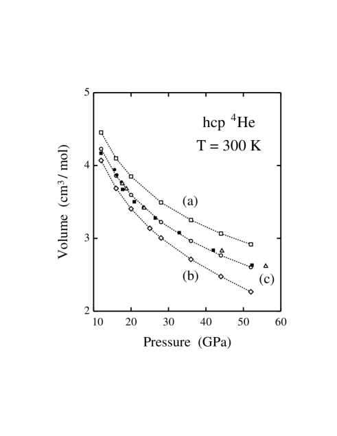
Figure 4: Equation of state $P$–$V$ of hcp ⁴He at 300 K, as derived from PIMC simulations for different interatomic potentials Herrero (2006). (a) Open squares: only two-body interactions with an Aziz-type potential Aziz et al. (1995); (b) open diamonds: two-body terms as in Ref. Aziz et al. (1995) and three-body interactions, as defined in Ref. Loubeyre (1987); (c) open circles: same potential as (b), but with the exchange three-body interaction rescaled by 2/3. Error bars of the simulation results are less than the symbol size. Dotted lines are guides to the eye. Open triangles show results obtained from PIMC simulations in the $NVT$ ensemble Chang and Boninsegni (2001), with the attractive exchange interaction rescaled as in (c). Black symbols show experimental data obtained by Mao et al. Mao et al. (1988) (filled circles) and Loubeyre et al. Loubeyre et al. (1993) (filled squares).

A question raised in this kind of computational studies has been the availability of effective potentials to describe helium at high pressures. This has been checked by analyzing the pressure-volume equation of state. The pressure dependence of the molar volume for hcp ⁴He is shown in Fig. 4 at 300 K Herrero (2006). Open symbols represent results of PIMC simulations with different interatomic potentials: (a) only two-body interaction with an Aziz-type potential Aziz et al. (1995) (squares); (b) two-body interaction as in Ref. Aziz et al. (1995) plus three-body terms as in Ref. Loubeyre (1987) (diamonds); (c) the same two-body potential and three-body interaction with the effective exchange part rescaled by 2/3, as proposed in Ref. Boninsegni et al. (1994) (circles). For comparison, we also display earlier results yielded by PIMC simulations in the $NVT$ ensemble Chang and Boninsegni (2001), with the exchange interaction rescaled by the same factor 2/3 (triangles). Filled symbols indicate experimental results obtained by Mao et al. Mao et al. (1988) (filled circles) and Loubeyre et al. Loubeyre et al. (1993) (filled squares). The interatomic potential (c) yields results for the equation of state of hcp ⁴He near the experimental data. For a given pressure, the only consideration of two-body terms predicts a molar volume larger than the experimental one. On the contrary, including both two- and three-body terms derived from ab initio calculations underestimates the volume of solid helium. This agrees with results obtained from PIMC simulations in the $NVT$ ensemble in Refs. Boninsegni et al. (1994); Chang and Boninsegni (2001). These results indicate that three-body terms are necessary to reproduce the high-pressure results, and are suitable for the pressure range nowadays experimentally available. However, this kind of effective interatomic potentials will probably yield a poor description of solid helium at very high pressures ($\gtrsim$ 60 GPa) Chang and Boninsegni (2001).

The compressibility of solid ³He and ⁴He in the hcp and fcc phases was studied by PIMC in Ref. Herrero (2008). Simulations were carried out in the canonical ($NVT$) and isothermal-isobaric ($NPT$) ensembles at temperatures between 10 and 300 K, showing consistent results in both ensembles. At a given pressure, the bulk modulus $B$ decreases as temperature rises. For pressures between 4 and 10 GPa, the change in $B$ was found to be in the order of 10%, when temperature increases from the low-$T$ limit to the melting temperature. Solid ³He is more compressible than ⁴He. At a given $T$, the difference between bulk moduli of both solids increases as pressure rises, but the relative difference between them decreases.

The coexistence between the hcp and bcc phases of solid ⁴He at fixed pressure was studied by Rota and Boronat Rota and Boronat (2011b) using PIMC simulations. They reported microscopic results for the energetic and structural properties of both phases. Differences between them were found to be small, with the exception of the static structure factor. When crossing the phase transition line, most appreciable changes are observed in the kinetic energy per particle and in the Lindemann ratio, both suggesting a less correlated quantum solid for the bcc crystal.

Turning now to the magnetic properties of condensed helium, solid ³He has been studied over the last four decades because at millikelvin temperatures, it is an almost pure spin-1/2 fermion system with a simple crystal structure. To study these properties, Candido et al. Candido et al. (2011) used PIMC simulations, and calculated ring exchange frequencies in the bcc phase of solid ³He, for densities ranging from melting to the highest stable density. Exchange frequencies were evaluated for two atoms and for long cycles including up to eight atoms. Using a fit to these frequencies, the contribution to the Curie-Weiss temperature, $\Theta_{CW}$, was calculated as well as an upper critical magnetic field, $B_{c2}$, for even longer exchanges, using a lattice Monte Carlo procedure. It was found that contributions from seven- and eight-particle exchanges make a significant contribution to $\Theta_{CW}$ and $B_{c2}$ at melting density.

Other phases of ⁴He, including amorphous solids, were studied by Boninsegni et al. Boninsegni et al. (2006a), who employed PIMC simulations based on a worm algorithm. This study included simulations that started from a high-temperature gas phase, which was subsequently ‘quenched’ down to $T$ = 0.2 K. The low-temperature properties of the system were found to crucially depend on the initial state, so that the disordered system was found to freeze into a superglass, i.e., a metastable amorphous solid displaying off-diagonal long-range order (ODLRO) and superfluidity.

As a final point in this brief survey of solid helium, we will consider the possibility of a supersolid phase, exhibiting nondissipative flow. The apparent discovery of a nonclassical moment of inertia in solid ⁴He by Kim and Chan Kim and Chan (2004) provided a possible experimental evidence for a supersolid, although the interpretation in terms of supersolidity of the ideal crystal phase has been questioned Kim and Chan (2012). This launched a series of path-integral studies, whose results in general were not compatible with the existence of a supersolid helium phase.

The possibility of superfluid behavior in bulk hcp ⁴He was investigated in Ref. Ceperley and Bernu (2004) by using PIMC simulations. Frequencies of ring exchange were calculated for the bosonic atoms of ⁴He. The obtained frequencies were fitted to a lattice model in order to examine whether such atoms could become a supersolid. It was found that the scaling with respect to the number of exchanging atoms is such that superfluid behavior is not expected to be observed in a perfect ⁴He crystal.

To study the order in solid ⁴He, Clark and Ceperley Clark and Ceperley (2006) carried out PIMC simulations to calculate the ODLRO, which for this purpose is equivalent to Bose-Einstein condensation. They did not find ODLRO in a defect-free hcp crystal at the melting density, and discussed their results in relation to proposed quantum solid trial functions, concluding that the solid ⁴He wave function has correlations which suppress both vacancies and Bose-Einstein condensation.

To estimate the onset temperature $T_{0}$ of Bose-Einstein condensation in ⁴He crystals presenting vacancies, the temperature dependence of the one-body density matrix was calculated by PIMC simulations in Ref. Rota and Boronat (2012). The temperature $T_{0}$ was found to depend on the vacancy concentration $X_{v}$, but did not follow the law $T_{0}\sim X_{v}^{2/3}$, expected for noninteracting vacancies. For $X_{v}=1/256$, it was obtained $T_{0}$ = 0.15 $\pm$ 0.05 K. Below $T_{0}$, vacancies did not behave as classical point defects, but became completely delocalized entities.

III.2 Heavier elements

Path-integral simulations have been used to study structural, thermodynamic, and vibrational properties of heavier noble-gas solids Cuccoli et al. (1997); Müser et al. (1995); Neumann and Zoppi (2000); Chakravarty (2002); Timms et al. (1996); Neumann and Zoppi (2002). This technique has turned out to be well-suited to analyze isotopic effects in different properties of these solids Müser et al. (1995). For example, the isotopic-mass dependence of the molar volume can be described well from this kind of simulations Herrero (1999, 2002). Moreover, in this context, several authors developed effective (temperature-dependent) classical potentials that reproduce accurately various properties of quantum solids Giachetti and Tognetti (1986); Feynman and Kleinert (1986); Cuccoli et al. (1992). Thus, Acocella et al. Acocella et al. (2000) applied an improved effective-potential Monte Carlo theory Acocella et al. (1995) to study thermal and elastic properties of noble-gas solids.

The capability of path-integral simulations to describe thermodynamic and structural properties of solids at low temperatures was studied in detail by Müser et al. Müser et al. (1995), considering noble-gas crystals as examples. They investigated solid Ar at constant volume, as well as isotope effects in the lattice parameter of ²⁰Ne and ²²Ne at zero pressure, with special emphasis on the convergence of their results at low temperatures. To reduce the systematic limitations due to finite Trotter and particle number, these authors proposed a combined Trotter and finite-size scaling. At very low temperatures much effort is necessary to avoid discretization effects in the phonon spectra, resulting in an artificial fast decrease in the specific heat as temperature is lowered. Better approximants than the primitive algorithm may be necessary to compute the exponent describing the vanishing of the heat capacity as $T\to 0$ (e.g., a Debye $T^{3}$ law for insulators). This calculation turns out to be difficult, because the exponent can only be measured at temperatures much lower than the Debye temperature of the solid. Taking all this into account, Müser et al. Müser et al. (1995) concluded that the lattice parameter and associated structural properties can clearly be resolved, as well as the isotope shift in the molar volume.

Given an interatomic potential, for volume $V$ and temperature $T$ the internal energy of a solid, $E(V,T)$, can be written in our context as Herrero (2002):

$$E(V,T)=U_{0}+U_{S}(V)+E_{\rm vib}(V,T)\,,$$ (67)

where $U_{0}$ is the minimum potential energy for the (classical) crystal at $T$ = 0 K, $U_{S}(V)$ is the elastic energy, and $E_{\rm vib}(V,T)$ is the vibrational energy: $E_{\rm vib}(V,T)=K(V,T)+U_{\rm vib}(V,T)$. For a given volume $V$, the classical energy at $T=0$ increases by an amount $U_{S}(V)$ with respect to the minimum energy $U_{0}$. This elastic energy $U_{S}$ depends only on the volume, but at finite temperatures and for the quantum solid, it depends implicitly on $T$ because of the temperature dependence of $V$ (thermal expansion). The elastic energy at low temperatures is basically due to the ‘zero-point’ lattice expansion.

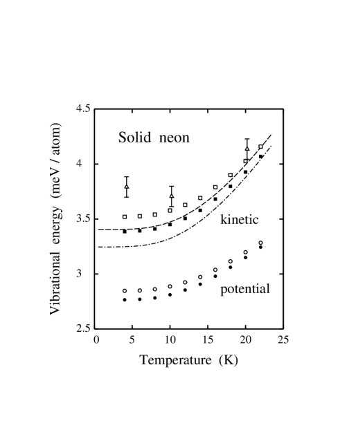
Figure 5: Temperature dependence of the vibrational energy of solid neon. Squares and circles correspond to kinetic and potential energy, respectively, as derived from PIMC simulations Herrero (2002). Open symbols, ²⁰Ne; black symbols, ²²Ne. Error bars of the simulation results are less than the symbol size. The dashed and dashed-dotted lines correspond to a Debye model for ²⁰Ne and ²²Ne, respectively, with $\Theta_{D}(^{20}{\rm Ne})$ = 70 K. Triangles are results for the kinetic energy of ²⁰Ne, obtained by Timms et al. Timms et al. (1996) from inelastic neutron scattering in solid neon with natural isotopic composition ($\overline{m}$ = 20.18 amu).

The vibrational energy, $E_{\rm vib}(V,T)$, depends on both $V$ and $T$, and can be obtained by subtracting the elastic energy from the internal energy. Path-integral simulations allow one to obtain separately the kinetic, $K$, and potential energy, $U_{\rm vib}$, associated to the lattice vibrations Gillan (1988). Both energies are shown in Fig. 5 for solid ²⁰Ne (open symbols) and ²²Ne (black symbols). Squares and circles correspond to $K$ and $U_{\rm vib}$ obtained in Ref. Herrero (2002). These results for the kinetic energy are close to those previously obtained from PIMC simulations with Lennard-Jones Cuccoli et al. (1993); Timms et al. (1996); Cuccoli et al. (1997) and Aziz Timms et al. (1996) interatomic potentials. Triangles in Fig. 5 indicate the kinetic energy of ²⁰Ne, found by Timms et al. Timms et al. (1996) from inelastic neutron scattering in solid neon with natural isotopic composition. The results of PIMC simulations indicate that the vibrational potential energy is smaller than the kinetic energy for both neon isotopes. Dashed and dashed-dotted lines in Fig. 5 represent $K$ and $U_{\rm vib}$ for ²⁰Ne and ²²Ne obtained from a harmonic Debye model for the lattice vibrations Herrero (2002).

Neumann and Zoppi Neumann and Zoppi (2002) performed PIMC simulations of liquid and solid Ne, in order to derive the kinetic energy as well as the single-particle and pair distribution functions of Ne atoms in condensed phases. The simulations were carried out using Aziz-type and Lennard-Jones potentials. The single-particle distribution function $n(r)$ was employed to derive the momentum distribution and to obtain an estimate of $K$. Differences between the considered potentials, as measured by the properties investigated, turned out to be not very large, especially when compared with the precision of the available experimental data.

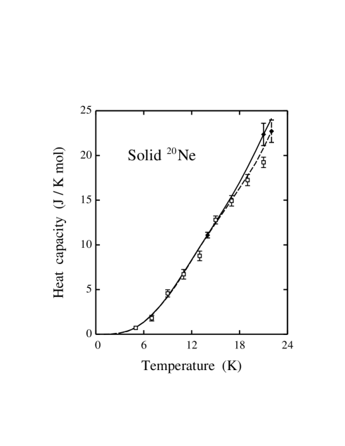
Figure 6: Heat capacity, $C_{P}$, of solid neon as a function of temperature. Squares indicate results of PIMC simulations for ²⁰Ne Herrero (2002). The continuous and dashed lines are experimental results for solid ²⁰Ne Somoza and Fenichel (1971) and for solid neon with natural isotopic composition Fenichel and Serin (1966), respectively. Error bars are given for three experimental points, indicated by black diamonds.

Path-integral simulations in the isothermal-isobaric ensemble have been also used to calculate the heat capacity $C_{P}$ of noble-gas solids. In Fig. 6 we present simulation results Herrero (2002) for ²⁰Ne at $P$ = 1 bar (open squares), to be compared with experimental data Somoza and Fenichel (1971) (solid line). For comparison, experimental results for natural neon Fenichel and Serin (1966) are shown as a dashed line. Results of the PIMC simulations follow closely the experimental data up to $T$ = 18 K, and at $T\geq$ 18 K they seem to be slightly lower. However, some experimental uncertainties have been reported for $T\gtrsim$ 18 K Somoza and Fenichel (1971).

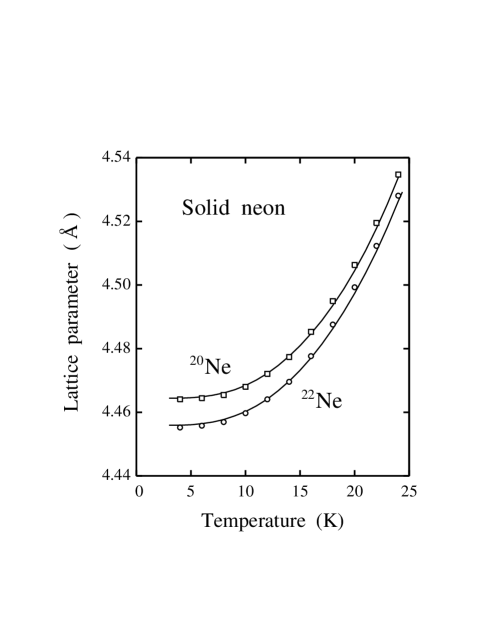
Figure 7: Temperature dependence of the lattice parameter of isotopically-pure crystals of solid neon, as derived from PIMC simulations for ²⁰Ne (squares) and ²²Ne (circles) Herrero (2002). Error bars are less than the symbol size. Solid lines represent results derived from x-ray diffraction experiments by Batchelder et al. Batchelder et al. (1968). Error bars of the experimental data are less than the line width.

As mentioned above, the thermal lattice expansion is an anharmonic effect that is well captured by path-integral simulations. The lattice parameter $a$ derived by the PIMC method in Ref. Herrero (2002) was found to follow closely the experimental data for ²⁰Ne and ²²Ne up to 24 K, as displayed in Fig. 7. Classical simulations yield a nearly linear temperature dependence for the lattice parameter Müser et al. (1995), which converges at low $T$ to the value corresponding to the minimum potential energy of the solid. One finds for the quantum solid ²⁰Ne a zero-temperature lattice parameter 4% larger than the classical limit Herrero (2002). This increase, due to anharmonicity of the zero-point motion, amounts to about twice the change in $a$ caused by thermal expansion between 0 K and the melting temperature of neon.

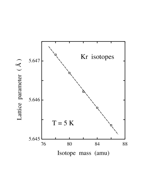
Figure 8: Lattice parameter of isotopically-pure Kr crystals as a function of isotopic mass at $T$ = 5 K and $P$ = 1 bar. Symbols indicate results of PIMC simulations Herrero (2003a). The dashed line is a least-square fit to the simulation results. Error bars are less than the symbol size.

The isotopic effect on the lattice parameter $a$ of other noble-gas solids (Ar, Kr, Xe) was studied in Ref. Herrero (2003a) as a function of temperature and pressure. A linear dependence of $a$ on the isotopic mass $m$ was found in all cases. As an example we show in Fig. 8 the parameter $a$ for some stable krypton isotopes at 5 K, as derived from PIMC simulations with a Lennard-Jones-type potential.

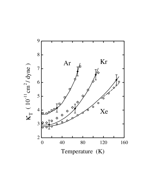
Figure 9: Isothermal compressibility $\kappa_{T}$ at $P$ = 1 bar as a function of temperature. Symbols indicate results derived from PIMC simulations for noble-gas solids with natural isotopic composition: Squares, Ar; diamonds, Kr; circles, Xe Herrero (2003a). Error bars of the calculated compressibilities are smaller than the symbol size. Lines represent experimental data obtained by different authors: Ar Peterson et al. (1966), Kr Losee and Simmons (1968). For Xe, the solid line is from Pollack (1964), whereas the dashed line represents more recent results from Granfors et al. (1981). Error bars are given for some experimental points, indicated by black diamonds.

The isothermal compressibility $\kappa_{T}$ can be derived from the volume fluctuations obtained in PI simulations in the isothermal-isobaric ensemble, as given by Eq. (37). In this way, $\kappa_{T}$ was derived for noble-gas solids in Ref. Herrero (2003a), and is presented here in Fig. 9 (symbols) as a function of temperature. Lines represent experimental data for crystals with natural isotopic composition Peterson et al. (1966); Pollack (1964); Granfors et al. (1981); Losee and Simmons (1968). The overall agreement between calculated and experimental results is good, given the uncertainty in the measurements Herrero (2003a). Comparison with the classical expectancy indicates that quantum effects give rise to an appreciable increase in the low-temperature compressibility: 19% for Ar, 9% for Kr, and 5% for Xe (for Ne, it is about 70% and depends on the isotope) Herrero (2002, 2003a).

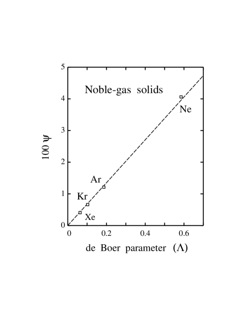
Figure 10: Low-temperature relative change in the lattice parameter, $\psi=(a_{\rm q}-a_{\rm cl})/a_{\rm cl}$, vs the de Boer parameter $\Lambda$ for noble-gas solids with fcc structure and natural isotopic composition. $a_{\rm q}$ and $a_{\rm cl}$ denote the quantum and classical lattice parameter for $T\to 0$. Symbols represent results derived from PIMC simulations Herrero (2003a). The line is a guide to the eye.

In connection with noble-gas solids, Chakravarty Chakravarty (2002) performed path-integral simulations to study structural and thermodynamic properties of quantum Lennard-Jones solids, as a function of the de Boer parameter $\Lambda=h/\sigma\sqrt{m\epsilon}$, which measures the quantum delocalization of the considered particles. These simulations revealed a strong dependence of the density on the parameter $\Lambda$. The lattice expansion of the quantum solids, with respect to their classical counterparts, is accompanied by an appreciable decrease in the binding energy. The relation between zero-temperature lattice expansion and the parameter $\Lambda$ for noble-gas solids was presented in Ref. Herrero (2003a), and is shown here in Fig. 10. The degree of solid-like order and the average coordination number were also found to depend markedly on $\Lambda$. Moreover, the calculated kinetic energy per particle indicates that a Lennard-Jones solid is far from the classical equipartition regime at temperatures as high as 70% of the melting temperature Chakravarty (2002). To assess the nature of the quantum-corrected energy landscape, effective pair potentials have been defined using the pair correlation function $g(r)$ of the quantum system Chakravarty (2011). For rising $\Lambda$, these effective potentials become increasingly softer, shallower, and of longer range, with the potential minimum shifted to larger distances.

Given the importance of anharmonic effects in noble-gas solids, PIMC simulations have been employed to assess the accuracy of harmonic or quasi-harmonic approximations for vibrational modes in these solids under pressure Herrero and Ramírez (2005). This allowed to quantify the overall anharmonicity of the lattice vibrations and its influence on several structural and thermodynamic properties. The vibrational energy $E_{\rm vib}$ increases with pressure, but this increase is slower than that of the elastic energy $U_{S}$ [see Eq. (67)], which dominates at high pressures. Results of these PIMC simulations indicated that the accuracy of the QHA to describe noble-gas solids increases as pressure is raised Herrero and Ramírez (2005). This is mainly a consequence of the relative importance of elastic and vibrational energy, as the latter becomes comparatively irrelevant as pressure rises. For large pressures, even a classical description of the vibrational modes can be precise enough to predict structural and thermodynamic properties of these solids. However, vibrational properties usually require the full quantum treatment, with the consideration of zero-point anharmonic effects.

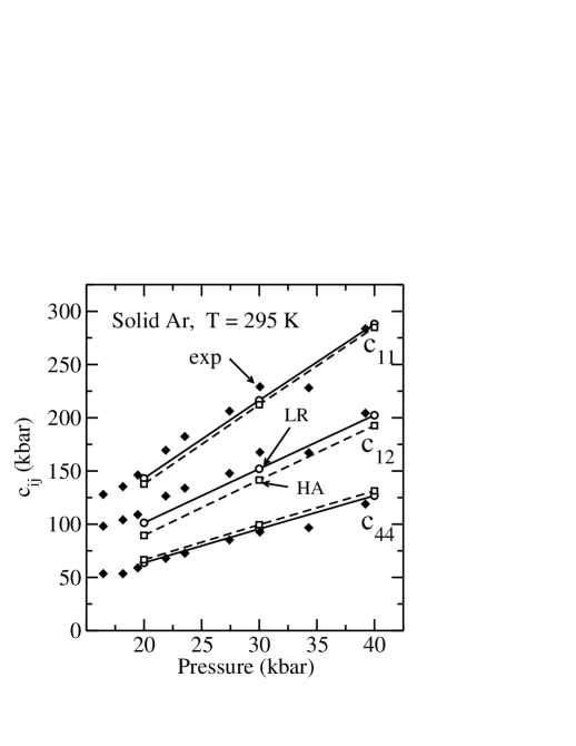
Figure 11: Pressure dependence of the elastic constants of solid Ar at 295 K. Results of the LR (circles) and harmonic approximation (HA, squares) procedures Ramírez and Herrero (2005) are compared to the adiabatic elastic constants determined by Brillouin spectroscopy Shimizu et al. (2001) (black diamonds). The lines are guides to the eye.

Another interesting application of path-integral simulations is the calculation of vibrational frequencies by using the static susceptibility tensor $\chi^{T}$ in the LR approach discussed in Sect. II.H. This method has been applied to study several properties of solid Ne and Ar as functions of pressure and temperature Ramírez and Herrero (2005). The LR approach predicts anharmonic shifts in the phonon frequencies in reasonable agreement to experimental data. This procedure has been also applied to calculate elastic constants of noble-gas solids from the propagation velocity of low-energy acoustic phonons. The temperature dependence of the elastic constants of solid Ne compares well with those derived from Brillouin scattering experiments Endoh et al. (1975); McLaren et al. (1975). For Ar, the pressure dependence of the elastic constants predicted by the LR method shows an overall agreement to experiment Shimizu et al. (2001), as presented in Fig. 11. Adiabatic elastic constants derived from Brillouin spectroscopy measurements are displayed by solid diamonds Shimizu et al. (2001). The values of $c_{11}$ and $c_{12}$ are slightly underestimated by the LR approach, maybe as a consequence of neglecting three-body forces Ramírez and Herrero (2005). The elastic constants obtained from a pure harmonic approximation are also plotted in Fig. 11. Elastic constants of solid Ar and ³He (hcp, fcc, and bcc) were also calculated by Schöffel and Müser Schöffel and Müser (2001) from PI simulations in the $NVT$ and $NPT$ ensembles. In particular, in the isothermal-isobaric ensemble they exploited the relationship between strain fluctuations and elastic constants, and found good agreement with available experimental data.

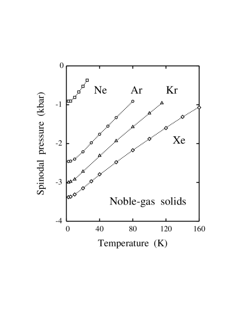
Figure 12: Calculated spinodal pressure for noble-gas crystals as a function of temperature Herrero (2003b). Squares, neon; circles, argon; triangles, krypton; diamonds, xenon. Error bars are less than the symbol size, and dotted lines are guides to the eye.

Turning to the thermodynamic properties of noble-gas solids, an interesting application of path-integral simulations consists in the assessment of quantum effects in their limits of mechanical stability. To this end, PIMC simulations in the isothermal-isobaric ensemble were carried out at negative pressure, which allowed to determine the solid-gas spinodal line Herrero (2003b). This line (spinodal pressure $P_{s}$ vs temperature) can be determined as the locus of points where the bulk modulus $B$ vanishes (the compressibility $\kappa_{T}$ diverges). The resulting data for the spinodal pressure are plotted in Fig. 12 as a function of temperature. In all cases, $P_{s}<0$, becoming more negative as the atomic mass of the noble gas increases. Quantum effects were found to affect appreciably the spinodal line at low temperatures, and make $P_{s}$ less negative than the classical expectancy. For $T\to 0$, this change in $P_{s}$ ranges from 43% for neon to 6% for xenon Herrero (2003b).

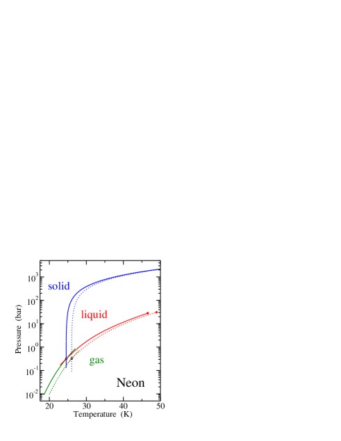
Figure 13: Phase diagram of natural neon in the pressure-temperature domain. Results are shown for the three coexistence lines between solid, liquid, and gas phases Ramírez and Herrero (2008). Continuous and dotted lines were derived from PIMC and classical MC simulations, respectively. Open circles represent the triple point and filled ones the critical point.

Free energy calculations based on PI simulations have been also employed to study the phase diagram of noble gases. For neon, in particular, this kind of simulations have demonstrated that free energy techniques, previously used in classical simulations, can be adapted and generalized to cover the case of quantum systems Ramírez and Herrero (2008); Ramírez et al. (2008a); Brito and Antonelli (2012). This includes the adiabatic switching (Watanabe and Reinhardt, 1990) and reversible scaling (de Koning et al., 1999) methods, which are based on algorithms where either the Hamiltonian, a state variable (pressure, temperature) or even an atomic mass are adiabatically changed along a simulation run (see Sect. II.I). Significant quantum effects were found in the phase diagram of neon at pressures below 2 kbar, where the solid-gas and liquid-gas coexistence lines are located Ramírez and Herrero (2008). The main quantum effect found for these two lines in the $P$–$T$ diagram is a shift of about 1.5 K towards lower temperatures. For the solid-liquid coexistence, the temperature shift decreases with pressure, from a value of 1.5 K at triple point conditions to 0.6 K at 2 kbar (see Fig. 13). This means that including quantum effects in the atomic dynamics of Ne in the solid and liquid phases lowers the melting temperature by 1.5 K compared to the classical result, i.e., a 6% of its actual value. A shift of 0.14 K in the triple-point temperature was found between ²⁰Ne and ²²Ne, in good agreement with experimental results Ramírez and Herrero (2008).

In connection with solid models including simple interatomic interactions, some path-integral simulations have been carried out for quantum hard-sphere solids. In particular, fcc, hcp, and bcc structures were recently studied in Ref. Sesé (2013) by PIMC, along with the fluid-solid coexistence lines. No significant differences between the relative stabilities of fcc and hcp lattices were found within the attained accuracy. Starting from a bcc solid, the simulations yielded either irregular lattices keeping some traces of the initial one, or spontaneous transitions to hcp-like lattices. It was discussed the relation between these transitions for quantum hard-sphere solids and solid-solid equilibria at low temperatures in real systems Sesé (2013).

IV Group-IV materials

Another important group of materials, for which path-integral simulations have been carried out, are those formed by elements of the group IV of the periodic table, in particular those with a cubic structure. This includes diamond and the well known semiconductors silicon, germanium, and silicon carbide (type 3$C$). Contrary to the noble-gas solids discussed above, where interatomic interactions are of van der Waals type, in group-IV materials the atoms are four-fold coordinated and connected by covalent bonds.

IV.1 Silicon

PIMC simulations of crystalline silicon have been performed in both the canonical ($NVT$) and isothermal-isobaric ($NPT$) ensembles Ramírez and Herrero (1993); Noya et al. (1996), using the empirical Stillinger-Weber potential. This allowed to study several finite-temperature properties of the material, such as potential energy, radial distribution function (RDF), and atomic delocalization. The simulations in the $NPT$ ensemble Noya et al. (1996) allowed to study properties of silicon such as lattice parameter, thermal expansion coefficient, heat capacity $C_{P}$, and bulk modulus. The calculated quantities showed an overall agreement with experimental data. These quantum simulations led to a good description of quantum effects like zero-point vibrations (mean-square displacements), and the results were found to converge to the classical limit at high temperatures. There appeared some deviations of the resulting vibrational energies when compared with the experimental ones, as the potential model seems to overestimate them.

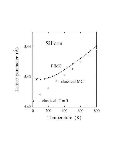
Figure 14: Temperature dependence of the lattice parameter $a$ for natural silicon. Data points were derived from PIMC simulations (filled squares) and in the classical limit (open squares) Herrero (1999). Experimental results Madelung (1982) are given as a dashed line. An arrow indicates the lattice parameter corresponding to the minimum potential energy of the crystal.

The relevance of anharmonicity and quantum effects on the properties derived from the PIMC simulations was addressed by comparison with the results of QHA calculations and classical simulations. A comparison of results derived in both quantum and classical approaches for several structural and thermodynamic properties of silicon was presented in Ref. Noya et al. (1996). In particular, the low-temperature lattice expansion due to anharmonicity of the zero-point vibration was found to be nonnegligible. In Fig. 14 we show the temperature dependence of the lattice parameter $a$ for $T$ up to 800 K. Filled and open circles are results of PIMC and classical MC simulations, respectively, whereas the dashed line corresponds to experimental measurements Madelung (1982); Hall (1961); Shah and Straumanis (1972). The results of the PIMC simulations follow closely the experimental data, but they do not reproduce the negative thermal expansion observed for silicon at $T<$ 100 K. This seems to be a drawback of empirical interatomic potentials, such as that employed in Refs. Noya et al. (1996); Herrero (1999). Classical MC simulations with the same effective potential yield an almost linear dependence of $a$ vs the temperature, with the lattice parameter converging at low $T$ to the value corresponding to the minimum potential energy of the silicon crystal (indicated by an arrow in Fig. 14). We note that the lattice expansion due to anharmonicity of the zero-point motion ($\Delta a$ = 0.007 Å) is in the order of the thermal expansion between 0 K and the Debye temperature of silicon ($\Theta_{D}\sim$ 650 K).

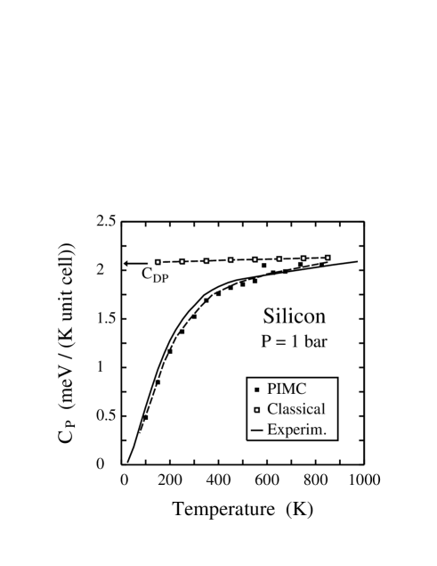
Figure 15: Temperature dependence of the heat capacity $C_{P}$ of crystalline silicon at $P=1$ bar. Filled and open squares are results derived from PIMC and classical MC simulations by numerical differentiation of the enthalpy values Noya et al. (1996). The dashed lines are smooth functions through the simulation data. The solid line shows the experimental temperature dependence of $C_{P}$ Gerlich et al. (1965); Shanks et al. (1963). An arrow indicates the $C_{P}$ value corresponding to the Dulong-Petit’s law, $C_{\text{DP}}=3Nk_{B}$, for $N=8$ atoms (the fcc unit cell of silicon).

In this context, a point of interest has been the capability of effective interatomic potentials to reproduce several properties of crystalline solids, and group-IV materials in particular. In general, this kind of potentials were designed to carry out classical simulations, so that its validity for quantum simulations is in principle not guaranteed. However, quantum path-integral results compared with experimental data much better than those derived from classical simulations, e.g., lattice parameter, bulk modulus and its pressure derivative, temperature dependence of the Grüneisen constant, and specific heat. At low temperatures, this could be expected for some quantities such as thermal expansion coefficient or specific heat, which should vanish for $T\to 0$, whereas usually they take finite (positive) values in a classical approximation. In Fig. 15 we display the heat capacity $C_{P}$ of silicon at $P$ = 1 bar, as derived from PIMC (black symbols) and classical MC (open squares) simulations Noya et al. (1996). Experimental results Gerlich et al. (1965); Shanks et al. (1963) are represented by a solid line. The agreement between values obtained in the PIMC simulations with the Stillinger-Weber potential and experimental data was satisfactory.

As shown above for noble-gas solids, an interesting application of path-integral simulations in the study of solids is the assessment of various isotopic effects. Maybe the most direct of these applications for PI simulations in the $NPT$ ensemble is the calculation of the isotopic effect in the crystal volume, which can be carried out in a nonperturbative way. Thus, the dependence of the lattice parameter $a$ of silicon on isotopic mass was studied by PIMC simulations in the isothermal-isobaric ensemble at ambient pressure Herrero (1999). At 300 K, the isotopic effect leads to a decrease of 0.8 and $1.6\times 10^{-4}$ Å in the lattice parameter of isotopically pure crystals of ²⁹Si and ³⁰Si, respectively, as compared to the solid with natural isotopic composition. At lower temperatures ($T\approx$ 50 K), this isotopic effect is about 50% larger than at room temperature. The fractional change in the lattice parameter of ³⁰Si with respect to natural silicon was found to be $\Delta a/a=-4.4$ and $-2.9\times 10^{-5}$ at 100 and 300 K, respectively. These results compare well with those derived from calculations using density-functional perturbation theory Pavone and Baroni (1994); Baroni et al. (2001). We emphasize that this dependence on isotopic mass results from a combination of the anharmonicity of the interatomic potentials and the quantum nature of atomic nuclei, which manifests itself in the zero-point vibrations (this isotopic effect does not appear in a classical model).

Another application of path-integral simulations in solids has been the study of amorphous materials. For amorphous silicon, in particular, quantum effects on the atomic delocalization were studied by PIMC simulations in the temperature range from 30 to 800 K Herrero (1998). In this material, the quantum delocalization was found to be appreciable vs. topological disorder, as seen from structural observables such as the RDF. At $T\approx$ 50 K, the width of the first peak in the RDF increases by a factor of 1.5 because of quantum effects. The overall anharmonicity of the solid vibrations at finite temperatures in amorphous silicon resulted to be significantly larger than in the crystalline material. Low-energy vibrational modes were found to be mainly located on coordination defects in the amorphous solid.

In connection with PI simulations of silicon, we mention that similar simulations have been carried out to study several structural and dynamical properties of silica polymorphs, in particular quartz Müser (2001); Rickwardt et al. (2001) and $\beta$-cristobalite Rickwardt et al. (2001).

IV.2 Germanium

As in the case of silicon, an application of path-integral simulations for germanium consisted in studying isotopic effects in this material. Thus, the dependence of the lattice parameter upon isotopic mass for isotopically pure Ge crystals was studied by PIMC simulations Noya et al. (1997a). At 50 K, the isotopic effect was found to yield an increase of $2.3\times 10^{-4}$ Å in the lattice parameter of ⁷⁰Ge with respect to ⁷⁶Ge, i.e., $\Delta a/a=4.1\times 10^{-5}$. Similar to silicon, a comparison of the simulation results with experimental data for ⁷⁴Ge indicated that effective interatomic potentials combined with path-integral simulations give a realistic description of this anharmonic effect in germanium.

The path-integral results were also compared to those derived from QHA calculations of the crystal vibrations. Within this approximation, the fractional change of the lattice parameter of ⁷⁴Ge respect to a crystal with atoms having the average mass of natural Ge amounts to $\Delta a/a=-9.2\times 10^{-6}$ in the limit $T\to 0$, which coincides within error bars with the results of the simulations Noya et al. (1997a). Data derived from the QHA slowly depart from those of PIMC simulations as temperature rises, since that approximation does not include the whole anharmonicity of the system, whose effects appear more clearly at high temperatures.

IV.3 Diamond

For diamond, path-integral simulations have been performed using different types of interatomic potentials, in particular effective Tersoff-type potentials Tersoff (1988) and tight-binding Hamiltonians. In Ref. Herrero and Ramírez (2001) several structural and thermodynamic properties of diamond were studied by PIMC simulations in the isothermal-isobaric ensemble, using a Tersoff-type potential. Such properties were investigated as functions of both temperature and hydrostatic pressure. The resulting lattice parameter, heat capacity, thermal expansion coefficient, and bulk modulus showed an overall agreement with experimental data. The relevance of quantum effects and anharmonicity on the properties derived from the path-integral simulations was estimated by comparison with results obtained from classical simulations with the same interatomic potential, as well as with those yielded by QHA calculations.

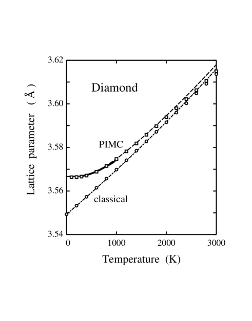
Figure 16: Temperature dependence of the lattice parameter $a$ of diamond at $P=1$ bar. The data shown were derived from PIMC (squares) and classical MC simulations (circles) Herrero and Ramírez (2001). Dashed and dashed-dotted lines were obtained in a quantum and classical QHA, respectively. Experimental results Madelung (1982) are displayed as a bold line.

In Fig. 16 we present the temperature dependence of the lattice parameter $a$ obtained in PIMC simulations (open squares), along with results of classical MC simulations (open circles) and experimental data (bold line). For comparison, a dashed line shows the lattice parameter obtained in a QHA with the Tersoff-type potential employed in Ref. Herrero and Ramírez (2001). This approximation yielded for the parameter $a$ values close to those obtained from the PIMC simulations, but at $T>$ 2000 K the $a$ values derived from the QHA gradually deviate from the PIMC data. From the results of these simulations, we emphasize that zero-point motion of carbon atoms causes an increase in the lattice parameter of $1.7\times 10^{-2}$ Å (a relative change of 0.5%) and a decrease in the bulk modulus by about 5%. These relative values are on the order of the precision obtained from ab initio electronic structure methods. This means that, at least for solids with light atoms, further improvements in electronic structure calculations cannot reduce the error bars in the computed values of structural observables, unless the effects associated to the quantum nature of atomic nuclei are taken into account.

The influence of quantum effects on the properties of solids is nontrivial in the presence of anharmonicity. For situations in which anharmonic effects can be treated perturbatively (i.e., low temperatures), the QHA gives a good description of physical observables, but this approximation becomes less accurate as temperature rises, as mentioned above in the case of heavier atoms (Si and Ge). Results of QHA calculations for several properties of diamond at room temperature are close to those yielded by PIMC simulations with a Tersoff-type potential Herrero and Ramírez (2001). This agreement is still good at pressures in the order of those attained in diamond anvil cells. Nevertheless, appreciable differences between QHA and PIMC results are found for diamond at temperatures higher than 1000 K, especially for the bulk modulus, thermal expansion coefficient, and heat capacity. At such high temperatures, anharmonic effects are enhanced and the QHA can only yield qualitative trends of the material properties.

Despite the limitations associated to employing empirical potentials originally optimized for classical simulations, a reasonable agreement was found between PIMC and experimental data for various finite-temperature properties of diamond, such as heat capacity and thermal expansion coefficient. For the heat capacity $C_{P}$, values slightly lower than the experimental ones were obtained, due to the rigidity of the Tersoff potential, which causes a hardening of vibrational modes. Nevertheless, this rigidity does not seem to affect the lattice parameter and thermal expansion. One expects that these shortages of effective potentials could be surmounted by using ab initio PI simulations, where the interatomic interactions are obtained from first-principles calculations.

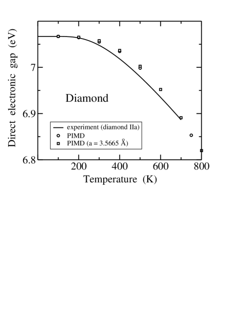
Figure 17: Temperature dependence of the direct electronic gap of diamond, obtained from PIMD simulations Ramírez et al. (2006). Open circles were derived from simulations that took into account the thermal expansion of the lattice. Open squares correspond to simulations where the cell volume was fixed to the equilibrium value at 100 K. The continuous line is a fit to the experimental data given in Ref. Logothetidis et al. (1992) for diamond IIa.

Diamond has been studied more recently by PIMD simulations using a tight-binding Hamiltonian to describe the electronic structure and total energy Ramírez et al. (2006). This kind of simulations are based on handling electrons and atomic nuclei as quantum particles, in the framework of the Born-Oppenheimer approximation. In this context, using the path-integral formalism for the nuclei allows one to assess the effect of zero-point vibrations and finite temperatures on the vibrational and electronic properties of solids. For diamond, this method predicted a reduction of the direct electronic gap by 0.7 eV (i.e., a 10%), as a consequence of the electron-phonon coupling mediated by zero-point vibrations. The direct gap was also predicted to decrease with temperature, in good agreement with experimental data available up to 700 K Ramírez et al. (2006) (see Fig. 17), as well as with theoretical results based on perturbation theory Zollner et al. (1992).

Anharmonic vibrational frequencies of diamond were obtained from the linear-response approach described in Sect. II.H. In particular, the temperature dependence of the zone-center optical phonon (at the $\Gamma$ point) was derived from PIMD simulations with a tight-binding Hamiltonian. A redshift of this phonon frequency was found, which turned out to be overestimated in comparison to experimental data at $T>$ 500 K Ramírez et al. (2006); Herchen and Cappelli (1991). Better agreement was found in the comparison of the elastic constants obtained from the simulations with experimental values derived from Brillouin scattering experiments Zouboulis et al. (1998).

Diamond has been also employed as benchmark for checking new simulation techniques related to path integrals. Thus, Ceriotti et al. Ceriotti et al. (2009) presented a method, based on a non-Markovian Langevin equation, aiming at including quantum corrections to the classical dynamics of ions in quasi-harmonic systems. These authors showed that fitting the correlation function of the noise, one can change the fluctuations in positions and momenta as functions of the vibrational frequency, and match them to reproduce the quantum-mechanical behavior. They applied this procedure to diamond and ice Ih, and found results in agreement with full PI simulations, but appreciably reducing the computational effort.

IV.4 Silicon carbide

Tight-binding Hamiltonians, similar to that employed for diamond, have been used to carry out PIMD simulations of cubic (3$C$) silicon carbide, as a function of pressure and temperature Ramírez et al. (2008b). These simulations were able to reproduce several experimental properties of 3$C$-SiC. Moreover, a comparison to classical simulations allowed to assess quantum effects in structural and thermodynamic properties, as well as to evaluate the separate contribution of each element (either C or Si) to various properties of the material.

The zero-point renormalization of the cell parameter $a$ (lattice expansion with respect to the classical value) derived from the PIMD simulations was found to be $\Delta a/a=2.5\times 10^{-3}$. This value is close to the sum of zero-point renormalizations obtained when only one type of atomic nuclei (either Si or C) is treated quantum mechanically Ramírez et al. (2008b). Moreover, the tight-binding potential employed in those simulations predicted a temperature dependence of the cell parameter, $a(T)$, in good agreement with experimental data. The main discrepancy was found for $T>$ 600 K, where the linear expansion coefficient was predicted to be about 8% larger than the experimental one. Other properties of 3$C$-SiC, such as the bulk modulus and its pressure derivative at room temperature displayed good agreement with the available experimental data.

As shown above for diamond, an interesting effect of the electron-phonon interaction is the decrease in the direct electronic gap of 3$C$-SiC for rising temperature. Results of the PIMD simulations for the gap showed satisfactory agreement with experimental data, although one observes that the tight-binding model employed in Ref. Ramírez et al. (2008b) tends to overestimate the magnitude of the electron-phonon interaction. At low temperatures, zero-point motion led to a gap renormalization $\Delta E_{0}=-0.69$ eV, which means a relative value $\Delta E_{0}/E_{0}=-0.10$.

PIMD simulations in the isothermal-isobaric ensemble have been also performed to investigate the dependence of the lattice parameter $a$ of 3$C$-SiC on isotopic mass Herrero et al. (2009). In these simulations, atomic nuclei were also treated as quantum particles interacting via a tight-binding-type potential. The isotopic effect was studied by considering separately changes in the C or Si mass, and assuming in each case for the other element the average mass of the natural isotopic composition. Considering changes in the C mass, the difference $\Delta a$ between lattice parameters of crystals with ¹²C and ¹³C at 300 K was found to amount to $2.1\times 10^{-4}$ Å. The effect due to Si isotopes is much smaller, and amounts to $3.5\times 10^{-5}$ Å when replacing ²⁸Si by ²⁹Si. These results of PIMD simulations can be interpreted in terms of a QHA for the lattice vibrations Herrero et al. (2009).

An important conclusion of this kind of simulations in group-IV materials is that they are well-suited to describe anharmonic effects related to the phonon-phonon interaction, as well as for the treatment of the electron-phonon coupling at finite temperatures. Thus, this type of simulations is an alternative to perturbational calculations, with the advantage of being also applicable in cases where a perturbational series might converge rather slowly. A prerequisite to account for phonon-phonon and electron-phonon interactions is a quantum description that includes both electrons and atomic nuclei.

V Molecular solids

V.1 Solid hydrogen

Solid hydrogen, a simple system consisting only of protons and electrons, exhibits remarkable properties under extreme conditions of pressure and temperature. Thus, a variety of structural phase transitions at high pressures has been found by various experimental and theoretical methods. Due to the light mass of hydrogen, solid H₂ and its isotopes solid deuterium (D₂) and tritium (T₂) appear as natural candidates to show significant nuclear quantum effects. In fact, in this case atomic nuclei are protons, deuterons, or tritons. The properties of hydrogen under extreme conditions have been recently reviewed by McMahon et al. McMahon et al. (2012).

Experimental studies based on static compression revealed three relevant phases of solid molecular hydrogen: phase I (high-temperature, relatively low-pressure phase), phase II (low-temperature, low-pressure phase), and phase III (high-pressure phase). These H₂ phases have been studied in recent years with path-integral simulations, using effective Zoppi and Neumann (1991); Cui et al. (1997, 2001, 2002) and ab initio potentials Biermann et al. (1998); Kitamura et al. (2000); Tsuneyuki et al. (2001); Geneste et al. (2012); Li et al. (2013). A new phase IV has been recently proposed Howie et al. (2012).

Kitamura et al. Kitamura et al. (2000); Tsuneyuki et al. (2001) reported quantum distributions of protons in phases I, II, and III. These H₂ phases were investigated by first-principles PIMD simulations, where the interatomic forces were given by DFT calculations. The resulting crystal structures were found to have different symmetries from those predicted by simulations where protons were treated classically. For phase II, an interesting result was that molecular rotation is hindered by quantum fluctuations of protons. This kind of quantum localization was rationalized by analyzing the potential energy surface for the molecular rotation, derived from DFT calculations Tsuneyuki et al. (2001).

The orientational order of H₂ molecules in these solid phases has been also studied from PIMC simulations in Ref. Cui et al. (2002), employing an empirical potential. The results of these simulations allowed to propose the following kinds of distribution of molecules: (I) orientationally disordered hcp; (II) orientationally ordered hcp with $Pa3$-type local orientational order; and (III) orientationally ordered orthorhombic structure of $Cmca$ symmetry. The transition between phases I and III was found to be essentially induced by thermal fluctuations, but quantum fluctuations were reported to be important in determining the transition temperature, by effectively hardening the intermolecular interaction Cui et al. (2001). From their results, these authors estimated the melting line for phase III. Other possible ordered structures at pressures $P\sim$ 150 GPa were analyzed in Ref. Surh et al. (1997).

The phase transition associated to orientational ordering in hcp H₂ was studied by Kaxiras and Guo Kaxiras and Guo (1994) using PIMC simulations with an effective potential obtained from DFT calculations. These authors analyzed short- and long-range angular correlations as well as the behavior of the corresponding order parameters, and found this transition to be of first order.

Classical and quantum ordering of protons in cold high-pressure solid H₂ have been recently investigated by Li et al. Li et al. (2013), at several points on the phase diagram, using ab initio PIMD simulations. These calculations revealed that the transition between phases I and II is strongly quantum in nature, which results from a competition between thermal plus quantum fluctuations that enhance molecular rotation, and anisotropic intermolecular interactions that hinder it. In this work, no evidence for the ‘quantum localization’ reported earlier Kitamura et al. (2000) was found (see above). The transition from phase II to III is more classical, since nuclear quantum motion plays a secondary role, and thus the transition is mainly controlled by the underlying potential energy surface. A $C2/c$ structure was proposed for phase III, which is now considered as the most likely candidate for this H₂ phase McMahon et al. (2012). Concerning the interatomic interactions, it was found that taking into account van der Waals forces improved the agreement between experiment and theory Li et al. (2013).

Biermann et al. Biermann et al. (1998) presented ab initio path-integral simulations of solid H₂ in the pressure range from 150 to 700 GPa. These authors compared results of the quantum-mechanical simulations with classical ones, which allowed them to assess nuclear quantum effects on the solid structure at different pressures. They showed that a QHA is insufficient to correctly describe the zero-point motion at megabar pressures. These simulations suggested the possibility that the structure of solid hydrogen at very high compression may be diffuse due to quantum effects, showing characteristics similar to fluid phases.

Turning to isotopic effects in these solid phases of hydrogen, PIMC simulations were carried out in Ref.  Runge et al. (1992) to study pressure-induced orientational ordering transitions in solid para-H₂, as well as in ortho-D₂ and para-T₂ (all of them with even angular momentum). These simulations were performed utilizing a potential energy derived from a local density approximation in the framework of DFT. At $T$ = 0, the transition pressure was found to change strongly as a function of the considered hydrogen isotope. In fact, pressures of 75, 26, and 12 GPa were obtained for H₂, D₂, and T₂, respectively. This procedure yielded phase diagrams for H₂ and D₂ in good agreement with experiment for orientational ordering up to pressures of about 100 GPa.

A strong isotope effect in phase II of solid H₂ and D₂ was reported by Geneste et al. Geneste et al. (2012). These authors investigated nuclear quantum motion at 80 K and pressures up to 160 GPa by first-principles PIMD calculations. An important result is that molecular orientations are well defined in phase II of D₂, but solid H₂ displays large and asymmetric angular quantum fluctuations, so that it is difficult to associate a single classical structure to this H₂ phase. The mechanism for the transition to phase III was also discussed in this contribution.

V.2 Ice

Condensed phases of water have been studied in recent years by means of PI simulations. For the different ice polymorphs, this kind of simulations have been mainly addressed to understand how the mass of the lightest atom, hydrogen, can influence the structural and thermodynamic properties of these solids. This includes consideration of isotopic effects in these properties, which can be nontrivial in some cases.

Computer simulation of water in condensed phases has a long history, that dates back to about 1970 Barker and Watts (1969); Rahman and Stillinger (1971). Studies of ice using path-integral simulations have been performed later by using mainly effective potentials, and were focused on structural and dynamic properties of several ice phases Gai et al. (1996a); Hernández de la Peña et al. (2005); Hernández de la Peña and Kusalik (2006); Paesani and Voth (2008); McBride et al. (2009). Different types of empirical potentials have been employed in these simulations Koyama et al. (2004); Jorgensen and Tirado-Rives (2005); Abascal and Vega (2005); Paesani et al. (2006); McBride et al. (2009). Many of them assume a rigid geometry for the water molecule (such as TIP4P and SCP models), and some others include molecular flexibility either with harmonic or anharmonic OH stretches (as the q-TIP4P/F model Habershon et al. (2009)). Also, in some cases the polarizability of the water molecule has been taken into account in the considered model potentials Mahoney and Jorgensen (2001). Moreover, some simulations of water using ab initio calculations for the electronic structure have appeared in the literature Fernández-Serra and Artacho (2006); Morrone and Car (2008); Li et al. (2011); Kong et al. (2012). Nevertheless, the hydrogen bonds present in condensed phases of water seem to be difficult to describe with available energy functionals, which causes that some properties are poorly reproduced by DFT simulations Yoo et al. (2009). This scenario is now changing by the development of new functionals that account for van der Waals interactions Corsetti et al. (2013).

Several properties of ice Ih have been investigated by using PI simulations with effective rigid-water potentials. Gai et al. Gai et al. (1996a) employed the SCP model to study ice Ih near the melting temperature, and concluded that nuclear quantum effects are appreciable at temperatures $T\lesssim$ 280 K, so that hydrogen bonds become effectively weaker. The TIP4P model was later employed to study hexagonal ice by centroid molecular dynamics Hernández de la Peña et al. (2005). The effect of quantization on the local structure, as measured by the radial and spatial distribution functions, as well as on the energy and lattice vibrational modes was presented. Comparison of results from quantum and classical simulations indicated that the increase in potential energy due to quantum motion is similar to that obtained by rising the temperature around 80 K. This study was extended to other rigid-water models available in 2006, and the results obtained for equilibrium and dynamical properties of ice showed no important discrepancies between the different potential models Hernández de la Peña and Kusalik (2006).

Later versions of the TIP4P potential, such as the so-called TIP4PQ/2005 model, have been used to investigate the influence of nuclear quantum delocalization on several ice phases. Path-integral simulations with this effective potential were found to reproduce well a number of physical properties of ice polymorphs, such as density, structure, heat capacity, and relative stability McBride et al. (2009); Vega et al. (2010). The TIP4PQ/2005 model was proposed in order to correct some deviations of the properties predicted by earlier TIP4P-type potentials with respect to experimental values. This question raised for rigid models of water is a problem generally appearing when performing path-integral simulations with effective potentials tailored to fit results of classical simulations to experimental data. In such cases, quantum effects may worsen the agreement with experimental results, because the effective potential already incorporates the effects of quantum zero-point motion by fitting its predictions to the actual experimental data. Thus, path-integral simulations may incur in a ‘double counting’ of these quantum effects, hence over-correcting the classical simulation data.

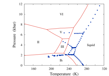
Figure 18: Phase diagram of water from PI simulations with the TIP4PQ/2005 model. Continuous lines correspond to the coexistence between phases, as derived from the simulations. Labels indicate liquid water and various ice polymorphs. Experimental results (dots) are also shown for comparison (from Ref. McBride et al. (2012), with permission of The Royal Society of Chemistry).

An interesting application of the TIP4PQ/2005 model consisted in calculating the phase diagram of water using PIMC McBride et al. (2012). The coexistence lines between different phases were traced out using thermodynamic integration, after calculating the free energies of liquid water and solid polymorphs. The resulting phase diagram was found to agree reasonably well with the experimental one, the former being displaced to lower temperatures by 15-20 K (see Fig. 18). In this work, the relevance of nuclear quantum effects on phase transitions was found to be significant. These quantum effects were rationalized in terms of the degree of tetrahedral ordering in the different ice polymorphs and the volume variation associated to each phase transition McBride et al. (2012).

An extension to other phases of water consisted in studying hydrate solid structures Conde et al. (2010). A classical description of hydrates is able to predict correctly the densities at $T>$ 150 K and the relative stabilities between the hydrates and ice Ih. Below 150 K, however, the inclusion of nuclear quantum effects was found to be necessary for a reliable description of the density, sublimation energy, heat capacity, and radial distribution function of these water phases.

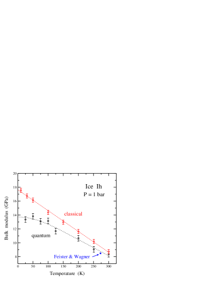
Figure 19: Bulk modulus of ice Ih as obtained from PIMD (open squares) and classical MD (open circles) simulations Herrero and Ramírez (2011). Error bars show the statistical uncertainty in the values of $B$ found from the simulations. A filled square represents the value obtained at 273 K from the equation of state derived by Feistel and Wagner Feistel and Wagner (2006) from experimental data. Lines are guides to the eye.

Among the effective potentials available for flexible water molecules, one of the most employed to carry out path-integral simulations of liquid water and ice has been the q-TIP4P/F potential, developed by Habershon et al. in 2009 Habershon et al. (2009). This potential was used in Ref. Herrero and Ramírez (2011) to analyze finite-temperature quantum effects in ice Ih from 25 to 300 K at atmospheric pressure. It was shown that this kind of quantum simulations are necessary to reproduce some properties of ice, that are not captured by classical simulations. Among these properties, PIMD simulations were able to reproduce the negative thermal expansion of hexagonal ice Ih at low temperatures. Also, these simulations gave the apparently anomalous decrease of the intramolecular O–H distance for increasing temperature. A good check of this interatomic potential was the calculation of macroscopic observables such as the bulk modulus $B$ shown in Fig. 19, where results from classical and PIMD simulations are presented Herrero and Ramírez (2011). In the classical simulations, $B$ is found to decrease approximately linearly as temperature is raised, and PIMD indicates that quantum ice Ih is ‘softer’ ($B$ is smaller). In the low-temperature limit a value $B=13.8\pm 0.4$ GPa was found, about 3.8 GPa smaller than the classical value, which means that quantum motion reduces the bulk modulus by more than 25%.

Isotope effects in ice Ih were analyzed from PIMD simulations by considering normal, heavy, and tritiated water Herrero and Ramírez (2011). In particular, it was studied the effect of changing the isotopic mass of hydrogen upon the kinetic energy and atomic delocalization in the crystal, as well as on structural properties such as interatomic distances and molar volume. For D₂O ice Ih at 100 K, it was found a decrease in the crystal volume and intramolecular O–H distance of 0.6% and 0.4%, respectively, as compared to H₂O ice. These simulations, however, did not reproduce the inverse isotopic effect in the crystal volume, observed in Ref. Röttger et al. (1994), i.e. the molar volume of D₂O ice derived from synchrotron x-ray diffraction is larger than that of H₂O ice (contrary to simpler solids, where heavier isotopes have smaller volume; see Fig. 7). This effect in ice has been later reproduced quantitatively by using DFT calculations in combination with a QHA for the solid vibrations Pamuk et al. (2012).

The isotopic effect in the melting temperature $T_{m}$ of ice Ih has been also calculated using path-integral simulations with the q-TIP4P/F potential Ramírez and Herrero (2010). At ambient pressure, these calculations predicted for D₂O and T₂O ice an increase in $T_{m}$ of $6.5\pm$ 0.5 K and $8.2\pm$ 0.5 K, respectively, vs H₂O ice. These temperature shifts show the same trend as experimental results, although the theoretical ones are larger in magnitude. This isotopic effect was rationalized by considering the coupling between intermolecular interactions and molecular flexibility in liquid water and ice Ramírez and Herrero (2010).

The kinetic energy of H and O nuclei in ice Ih at $P$ = 1 bar was studied as a function of temperature in Ref. Ramírez and Herrero (2011). Results obtained for the proton kinetic energy in hexagonal ice compared well with data derived from deep inelastic neutron scattering experiments, although some discrepancies were observed in the case of liquid water. (The data analysis of some of these experiments in water has been controversial Soper (2009); Pietropaolo et al. (2009).) The temperature dependence of $K_{\rm H}$ predicted by the q-TIP4P/F model for ice Ih was found in good agreement with results of path-integral simulations using ab initio DFT Ramírez and Herrero (2011). Comparing calculated values of $K_{\rm O}$ and $K_{\rm H}$ in water and ice at isothermal conditions, it was shown that the larger results always correspond to the solid phase. This fact determines the sign of the isotopic shift in the melting temperature of ice upon isotopic substitution of either H or O atoms. In both cases the model predictions agreed to experimental data Ramírez and Herrero (2011).

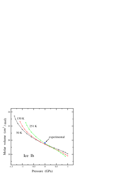
Figure 20: Molar volume of ice Ih as a function of pressure, as derived from PIMD simulations at various temperatures: 50 K (squares), 150 K (circles), and 251 K (triangles) Herrero and Ramírez (2011). Error bars are in the order of the symbol size. Lines are guides to the eye. A solid diamond represents experimental data from Refs. Ginnings and Corruccini (1947); Dantl and Gregora (1968) at atmospheric pressure and 273 K.

Another application of path-integral simulations with a flexible-water model (q-TIP4P/F) has been an study of ice Ih under pressure Herrero and Ramírez (2011). Positive (compression) and negative (tension) pressures were considered, which allowed to approach the limits for the mechanical stability of hexagonal ice. Several structural and thermodynamic quantities were studied as functions of pressure: crystal volume, bulk modulus, interatomic distances, atomic delocalization, and kinetic energy. The overall agreement with available experimental data was good. In Fig. 20 we show the pressure dependence of the molar volume at three different temperatures: 50, 100, and 251 K. At a given temperature, one observes the common volume decrease for increasing pressure ($dV/dP<0$), and in most of the considered pressure region one has $d^{2}V/dP^{2}>0$. Nevertheless, around $P$ = 0.5 GPa it was found a change in the trend of the first derivative, as indicated by the existence of an inflection point with $d^{2}V/dP^{2}=0$. This change in the trend of the $P$–$V$ curve has been argued to be related with to the proximity of ice amorphization Mishima et al. (1984); Sciortino et al. (1995); Strässle et al. (2004). It is also remarkable that the volume-pressure curves cross at $P\sim$ 0.2–0.3 GPa, as discussed in Herrero and Ramírez (2011). This anomalous behavior of the crystal volume as a function of temperature seems to be due to the negative sign of the Grüneisen parameter for TA vibrational modes in ice Ih Strässle et al. (2004).

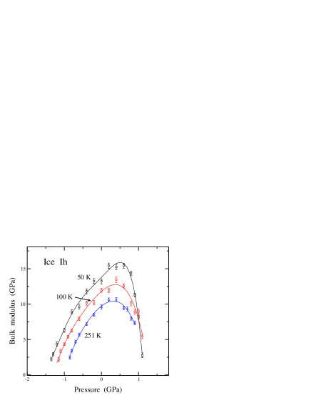
Figure 21: Pressure dependence of the bulk modulus of ice Ih as obtained from PIMD simulations at several temperatures: 50 K (squares), 150 K (circles), and 251 K (triangles) Herrero and Ramírez (2011). Error bars show the statistical uncertainty in the values of $B$ found from the simulations. Lines are guides to the eye.

In connection with the pressure dependence of the crystal volume, the bulk modulus $B$ is also expected to show some related anomalies. Thus, at positive and negative pressures, $B$ was found to extrapolate to zero (the compressibility diverges) at the corresponding spinodal pressure $P_{s}$, which depends on temperature (see Fig. 21). In this respect, it was found that nuclear quantum effects reduce the metastability region of ice Ih, for both negative and positive pressures Herrero and Ramírez (2011).

Notwithstanding the volume reduction for increasing pressure, the interatomic distances in ice were found to change in a peculiar way. Thus, the distance between oxygen atoms in adjacent molecules decreases as pressure is raised, but the intramolecular O–H distance becomes larger (see Fig. 22). This is due to the hydrogen bonds between contiguous molecules, which become stronger as the volume (or O–O distance) is reduced, causing a weakening of the intramolecular O–H bonds Herrero and Ramírez (2011).

Amorphous ice has been likewise investigated by path-integral simulations. Thus, structural and thermodynamic properties of high-density amorphous (HDA) ice were studied by PIMD simulations in the isothermal-isobaric ensemble, using the q-TIP4P/F potential model Herrero and Ramírez (2012). Quantum nuclear motion was found to affect several observable properties of the amorphous solid. At $T$ = 50 K, the molar volume of HDA ice was found to increase by 6%, and the intramolecular O–H distance rose by 1.4% due to quantum motion. Moreover, PIMD simulations showed a broadening of the peaks in the RDFs, as compared with classical MD simulations. For different isotopes, changes in the RDFs of HDA ice were observed. In particular, the width of the peaks in the O–H RDF was found to depend on the considered hydrogen isotope, but the general features of this RDF were substantially the same for H₂O and D₂O ice.

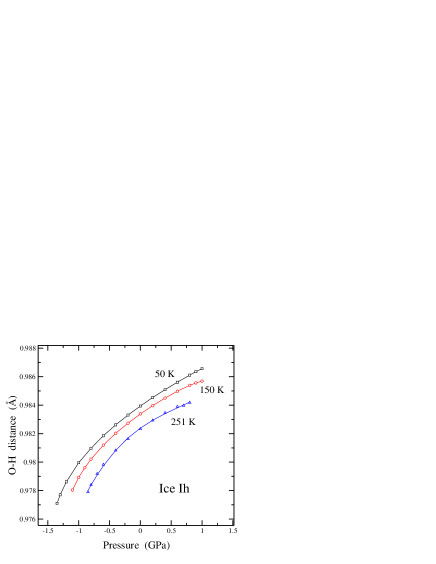
Figure 22: Pressure dependence of the mean intramolecular O–H distance, as derived from simulations of ice Ih Herrero and Ramírez (2011). Open symbols represent results of PIMD simulations at different temperatures: 50 K (squares), 150 K (circles), and 251 K (triangles). Error bars are in the order of the symbol size. Lines are guides to the eye.

These conclusions contrast with those of earlier PIMC simulations in the $NVT$ ensemble, using the SPC/E rigid-water model Gai et al. (1996b). In these simulations, the structure of H₂O amorphous ice was found to be significantly different from that in D₂O ice, and this difference was attributed to the larger quantum delocalization of the protons, as compared to the deuterons. These authors argued that the hydrogen bonding network that is present in D₂O amorphous ice either disappears or is totally mixed with the second nearest-neighbor shell. Apart from the constant volume employed by Gai et al. Gai et al. (1996b) in their simulations vs the constant pressure employed in PIMD simulations with the q-TIP4P/F potential, the main difference between both kinds of calculations was the interatomic potential: rigid molecules in Ref. Gai et al. (1996b) vs flexible molecules in Ref. Herrero and Ramírez (2012). Nevertheless, it does not seem straightforward to find a convincing explanation why rigid molecules should yield very different structures for H₂O and D₂O amorphous ice, as suggested by the results of Gai et al.

Some measurements of the momentum distribution in water and ice revealed that protons are in a considerably softer potential in ice Ih than in water or the free monomer, which is compatible with the large redshift observed in the vibrational spectrum of ice. Burnham et al. Burnham et al. (2006) showed that many water models, which consider the intramolecular potential as unchanged by the hydrogen bonding cannot reproduce the momentum distribution. Moreover, although they can substantially reproduce the redshift, they are unable to explain the large rise in intensity observed in the infrared spectrum when going from the water monomer to ice Ih. To correct these limitations, an empirical flexible and polarizable water model (TTM4-F) has been developed Burnham et al. (2008). Using PIMD simulations, this model was found to give an improved description of the momentum and position distributions, as well as the infrared spectrum. It was shown that the over-rigidity of the OH stretch and the underestimation of infrared intensity, observed for other empirical models, are connected to the failure to reproduce the correct monomer polarizability surface.

More recently, Lin et al. Lin et al. (2011) analyzed the effective potential experienced by protons in ice Ih from PI and phonon calculations. They found an anisotropic quasi-harmonic effective potential with three distinct principal frequencies corresponding to different molecular orientations. Anharmonicity in the ground-state dynamics of protons turned out to be appreciable. From these calculations, it was concluded that the full momentum distribution is required for a reliable comparison with experimental results.

Among other applications of PI simulations to condensed phases of water, quantum motion of H₂O molecules has been shown to appreciably affect the surface premelting of ice Ih Paesani and Voth (2008). This behavior was revealed by calculating structural and dynamical properties of the ice surface below the melting point. Results of PIMD and centroid molecular dynamics simulations with a polarizable and flexible water model predicted the existence of a quasi-liquid phase extending about 10 Å into the bulk, in line with results of optical ellipsometry measurements. Surface disorder in the topmost layers of the quantum ice was found to persist at temperatures of about 10–20 K lower than its classical counterpart.

Effective potential models for condensed phases of water usually treat the H₂O molecules as well-defined unbreakable entities, connected by H-bonds. However, high-pressure phases such as ice X, include symmetric O$-$H$-$O bonds, thus preventing their modeling with those empirical potentials. This drawback does not affect ab initio potentials, where in principle any geometry or bonding configuration can be considered. Thus, Benoit et al. Benoit et al. (1998) investigated the role of quantum effects in proton ordering and hydrogen-bond symmetrization in high-pressure phases of ice, by using PIMD simulations with an internuclear interaction given by ab initio DFT. They found a sequence of transitions from antiferroelectric ice VIII to paraelectric (proton disordered) ice VII, and finally to symmetric ice X. Nuclear quantum effects were found to influence these transitions: the antiferroelectric disordering transition is affected by proton tunneling, whereas the symmetrization transition is influenced by zero-point motion. The coordination of H in ice X, with a unimodal proton distribution centered at the O–O midpoint, was explained on the basis of an effective potential for hydrogen. This potential evolves from a double-well shape at lower pressures to a single-well shape with a stronger proton localization at higher pressures. Thus, this kind of simulations have allowed to study the shape of the proton-transfer potential between a donor and an acceptor molecule in ice Benoit et al. (1999).

More recently, the momentum distribution of protons in high-pressure ice phases was studied by Morrone et al. using ab initio PIMD Morrone et al. (2009). They found that the symmetric H-bonded phase (ice X) is characterized by a momentum distribution narrower than phases containing the usual intramolecular covalent OH bonds, such as ice VIII, in agreement with experimental findings. The transition to the tunneling regime displays similarities to some aspects observed in experiments on confined water. The results of these simulations were rationalized with a one-dimensional double-well potential model, that captures some of the effects observed in the simulations. This allowed to distinguish between ground state and mixed state tunneling effects in the proton dynamics Morrone et al. (2009).

V.3 Other molecular solids

Path-integral simulations have been also carried out to study other molecular solids. We present here a few of them. Solid nitrogen was investigated by Presber et al. Presber et al. (1998) using PIMC simulations in the isothermal-isobaric ensemble. They assumed an N₂ crystal composed of rigid molecules interacting via Lennard-Jones and electrostatic potentials. The effect of quantum fluctuations on molar volume, energy, and temperature for the orientational order/disorder transition was studied as a function of pressure. The low-temperature molar volume and energy derived from the PIMC simulations were close to the corresponding experimental values, in contrast to classical simulations. At $P=0$, the transition temperature from a high-temperature orientationally disordered cubic phase to a low-temperature phase with $Pa3$ structure was found to be reduced by about 11% as a consequence of quantum motion. For increasing pressure, the transition temperature rises and the difference between classical and quantum values is reduced.

The quantum rotator phase transition in solid methane was analyzed in Ref. Müser and Berne (1996) by using PIMC simulations. With this purpose, an efficient quantum propagator for asymmetric tops was developed. Quantum fluctuations were found to reduce the transition temperature from a high-temperature plastic phase to a low-temperature orientationally ordered state.

The temperature dependence of several physical properties of crystalline polyethylene at $P$ = 0 was studied by using self-consistent quasi-harmonic lattice dynamics Rutledge et al. (1998), as well as classical and PIMC simulations Martonak et al. (1998); Rutledge et al. (1998). Special emphasis was laid upon the classical approximation, the onset of anharmonicities in the atomic dynamics, not captured by the QHA, and finite size effects. It was shown that quantum effects are significant for $T\lesssim$ 300 K, and above 250 K (about 2/3 of the melting temperature) the QHA becomes increasingly inadequate. Taking into account the computational costs, it was concluded that quasi-harmonic lattice dynamics may be a very efficient alternative to study solid polyethylene at $T<$ 250 K.

VI Point defects in solids

Point defects in solids have been investigated in the last decades using different experimental and theoretical techniques. Over the last 20 years, path-integral simulations have been applied to study the structure (geometry) and dynamics of this kind of defects in a variety of materials. Several works have been devoted to hydrogen-like impurities, since they are expected to show relevant nuclear quantum effects. Other applications have included heavier impurities, such as oxygen in semiconductors Ramírez et al. (1997) and group-III elements in solid hydrogen Krumrine et al. (2000); Mirijanian et al. (2002).

VI.1 Structure

Several path-integral simulations have dealt with atomic hydrogen in silicon and diamond. Thus, finite-temperature properties of isolated hydrogen and deuterium impurities in crystalline silicon were studied by the PIMC method, in the temperature range from 50 to 600 K Herrero and Ramírez (1995). Interactions between Si atoms were modeled by an effective Stillinger-Weber potential, and the Si–H interaction was parameterized by following the results of pseudopotential-DFT calculations. Hydrogen and deuterium were found to be stable at the bond-center (BC) site, midway between two adjacent Si atoms. Average values of the kinetic, $\langle K\rangle$, and potential, $\langle U\rangle$, energy of the defect were compared with those expected for the impurity within a harmonic approximation. At low temperatures, $\langle K\rangle$ is larger than $\langle U\rangle$, as a consequence of the strong anharmonicity of the potential surface for the impurity around the BC site.

Similar simulations were carried out for muonium in crystalline Si, which behaves for this purpose as a light pseudo-isotope of hydrogen. In contrast to hydrogen, the same interatomic potential model predicted muonium to be delocalized in the interstitial region. This mass-induced effect was argued to be a consequence of the uncertainty principle, that prevents localization of muonium at the BC site due to an increase in its kinetic energy Ramírez and Herrero (1994). These hydrogenic impurities in silicon were later studied by the PIMD method using DFT-based interatomic potentials Miyake et al. (1998). It was shown that muonium has a high density at the center of the silicon cage (the so-called T site) due to quantum effects, i.e., far from the BC site found for hydrogen.

A similar PIMC study was carried out for hydrogenic impurities in boron-doped silicon, using empirical potentials for the Si–Si and Si–B interactions, and a potential for hydrogen parameterized from DFT calculations Noya et al. (1997b). Isotopic effects on the properties of B–H complexes were studied by considering also B–D pairs. Thus, it was analyzed the influence of the isotope mass on the impurity energy, atomic delocalization and lattice relaxation. The reorientation rate of these complexes was obtained from quantum transition-state theory, based on the PI centroid formalism Noya et al. (1997c). A change in the Arrhenius plot for the jump rate of hydrogen was obtained at $T\sim$ 60 K, indicating a crossover from thermally activated quasi-classical motion over a barrier to thermally assisted quantum tunneling, in line with experimental data. For deuterium, a break of the Arrhenius law was found at $T\sim$ 35 K. These PI simulations showed that the defect complex undergoing quantum tunneling consists of hydrogen, boron and the nearest silicon atoms, rather than the hydrogen atom alone.

With respect to hydrogen-like impurities in diamond, PIMD simulations in the canonical ensemble have been performed to study isolated hydrogen, deuterium, and muonium in this material Herrero et al. (2006). Finite-temperature properties of these point defects were analyzed in the range from 100 to 800 K. The interatomic interactions were modeled by a tight-binding potential fitted to DFT calculations. The most stable position for these hydrogenic impurities was found to be a BC site between carbon atoms, in agreement with earlier theoretical calculations. Vibrational frequencies associated to the defect complexes were calculated within the LR approach discussed in Sect. II.H. The resulting frequencies displayed a large anharmonic effect in the impurity vibrations at the BC site, causing a hardening of the vibrational modes with respect to a harmonic approximation. Quantum zero-point motion was found to produce an appreciable shift of the defect level in the electronic gap, as a consequence of electron-phonon interaction Herrero et al. (2006).

Turning to molecular hydrogen as an impurity in solids, PIMD simulations have been carried out to analyze isolated H₂ molecules in silicon and graphite Herrero and Ramírez (2009a, 2010). In these works, tight-binding-type potentials were used to model the interatomic interactions. For H₂ in silicon, the most stable position was found at the interstitial T site with the hydrogen molecule rotating freely in the Si cage Herrero and Ramírez (2009a). The H–H stretching frequency derived from the LR approach showed a large anharmonic effect, resulting to be softened with respect to a harmonic approximation by about 300 cm^-1. Moreover, the coupling between rotation and vibration was found to give rise to an important decrease in this frequency for rising temperature.

Using the same procedure, finite-temperature properties of H₂ molecules adsorbed between graphite layers were analyzed in the temperature range from 300 to 900 K Herrero and Ramírez (2010). In its lowest-energy position, the H₂ molecule was found to be disposed parallel to the sheets plane. At finite temperatures, the molecule explored other orientations, but its rotation turned out to be partially hindered by the adjacent graphite layers. For the H–H stretching vibration, a frequency of 3916 cm^-1 was found at 300 K, more than 100 cm^-1 lower than the frequency corresponding to an isolated H₂ molecule (in vacuo). For D₂ molecules in graphite, a stretching frequency of 2816 cm^-1 was obtained at room temperature, which compared with the H₂ frequency gives an isotopic ratio of 1.39, close to $\sqrt{2}$.

Going to heavier impurities in solids, a well-known case is that of oxygen in semiconductors, and silicon in particular. This is an archetypal example of isolated impurities in solids showing low-energy highly-anharmonic quantum dynamics, a question for which path-integral simulations have turned out to be a well-suited tool. In particular, interstitial oxygen in silicon was studied by PIMC simulations in Ref. Ramírez et al. (1997). An interesting problem arises since the definition of a geometry for this defect is conditioned by the presence of a large anharmonicity. This means that the configuration with minimum potential energy may not correspond to a maximum in the probability density of the impurity atom. In fact, the minimum energy corresponds to a bent Si-O-Si configuration, whereas the PIMC simulations yielded the maximum density for oxygen at a BC site, midway between silicon atoms. In contrast, for the oxygen impurity in germanium, a different geometry is found and the Ge-O-Ge structure turns out to be puckered, with O rotating around the Ge-Ge axis Artacho et al. (1997).

We now turn to atomic impurities in molecular solids. First, we consider B and Al impurities in solid para-H₂. The equilibrium properties of a boron atom trapped in solid para-H₂ were investigated by Krumrine et al. Krumrine et al. (2000) using PIMD simulations. Due to its singly filled $2p$ orbital, the B atom interacts anisotropically with the hydrogen molecules in the solid. To assess the effect of this electronic anisotropy, these authors performed simulations in which an orientation-averaged B-H₂ potential was used. It was found that small distortions of the lattice allow for an energetically favorable orientation of the $2p$ orbital, even in the absence of a vacancy. When the B impurity is located near the surface, the spherically-averaged potential gives a very different description from the case of the anisotropic potential Krumrine et al. (2000).

For Al impurities in para-H₂, it was particularly considered the interaction between these impurities and vacancies in the solid Mirijanian et al. (2002). In the presence of a vacancy, the orientation-dependent Al-H₂ potential causes the Al atom to displace to the midpoint between its substitutional site and the vacancy. Thermodynamic results indicated that the presence of a neighboring vacancy stabilizes the Al impurity much more than in the case of the B impurity Krumrine et al. (2000).

Apart from B and Al, isolated Li impurities in solid para-H₂ and ortho-D₂ have been studied by Scharf et al. Scharf et al. (1993) using PIMC simulations in the isothermal-isobaric ensemble. These calculations predicted the impurities to occupy preferentially a three-vacancy trapping site in para-H₂, whereas in ortho-D₂ a four-vacancy trapping site seemed to be favored. For comparison, a variational Einstein model predicted that the four-vacancy trapping site is favorable in both para-H₂ and ortho-D₂ Scharf et al. (1993). The effect of pressure on the trapping site structures and adsorption spectra of Li in solid H₂ has been studied later by PIMC simulations Ma et al. (2001). The applied pressure was found to cause a reduction in the Li–H₂ and H₂–H₂ distances, but no appreciable rearrangement of the local structure around the Li impurity was observed for pressures up to 4.8 GPa.

Other point defects, such as vacancies in solid ⁴He have been also studied using PIMC simulations Clark and Ceperley (2008). A relevant question in this case is the energy necessary to create a single vacancy, which was found to be 11.5 K (0.99 meV). As expected, the number of atom exchanges in the system increases with the vacancy concentration. As a result, it was observed in the simulations that the solid becomes unstable to melting whenever more than a few percent of the crystal sites become vacant. It was shown that vacancies behave in an attractive way, and the simulations allowed to quantitatively study the inter-vacancy attraction.

VI.2 Diffusion

Concerning impurity diffusion in solids, two methods based on path integrals have been mainly applied to calculate jump rates and diffusion coefficients. One of them is based on quantum transition-state theory, as described above in Sect. II.G. Other methods rely on real-time MD simulations, where the ring-polymers describing the quantum particles move according to the forces derived from interatomic interactions, giving an approximation to the actual quantum dynamics Cao and Voth (1994a, b); Jang and Voth (1999); Craig and Manolopoulos (2004); Pérez et al. (2009); Habershon et al. (2013).

One of the earliest applications of atomistic PI simulations of solids was the work by Gillan Gillan (1987b, 1988), devoted to study hydrogen-like impurities in metals. In particular, he considered hydrogen, deuterium and muonium in Pd and Nb, based on empirical interaction models, and carried out PIMC simulations to study the influence of quantum effects on the properties of these isolated impurities. Results for the density distribution of D, H, and the positive muon over the unit cell showed an important increase of quantum effects along this series. Gillan calculated effective diffusion barriers for these point defects, and found that they change appreciably with the impurity mass. The calculated diffusion coefficient for H in Nb displayed an experimentally observed break in the Arrhenius slope at 250 K, which was interpreted as a cross-over from classical (high $T$) to quantum (low $T$) behavior. Moreover, calculations of the activation energy for diffusion showed the relevance of excited states at high temperature, suggesting that the hydrogen diffusion is approximately classical in this regime Gillan (1987b, 1988).

For hydrogen-like impurities in silicon, QTST was applied to study the jump rate of atomic hydrogen and deuterium Herrero (1997). In this case the interatomic interactions were modeled with potentials similar to those described for this system in Sect. IV.A. The hydrogen jump rate was found to follow an Arrhenius law, describable with classical transition-state theory at $T>$ 100 K. At $T\sim$ 80 K, a change in the slope of the Arrhenius plot was obtained for hydrogen, as expected for the onset of a diffusion regime controlled by phonon-assisted tunneling of the impurity. In these calculations, no change of slope was observed for deuterium in the studied temperature range down to 40 K.

Figure 23: Probability density for hydrogen in silicon, as derived from PIMC simulations with the path-centroid of the impurity fixed at the saddle point C^∗ Herrero (1997). Shown is the projection of the density along the [110] crystal direction. Continuous line, 200 K; dashed line, 70 K; dotted line, 40 K. The appearance of two well-defined maxima in the probability density at $T$ = 40 K is an indication of impurity tunneling.

In this context it is interesting to analyze the probability distribution of the hydrogenic impurities with the path-centroid fixed at the saddle point (the so-called C^∗) in the diffusion barrier. This provides information on the delocalization of the considered particle in the two potential wells, corresponding to two adjacent energy minima (BC sites). A projection of the probability density of hydrogen in silicon along the [110] crystal direction is displayed in Fig. 23. The spatial distribution of the impurity broadens as temperature is lowered, and eventually its shape changes from a single maximum around the saddle point to a bimodal distribution, which is a fingerprint of quantum tunneling Herrero (1997); Mattsson et al. (1993). This change in the distribution of the quantum paths as temperature decreases, is associated to a transition from semiclassical motion over the effective barrier to quantum tunneling through the barrier. The effect of the impurity mass on the quantum delocalization is important at low temperatures, as shown in Fig. 24, where dashed and continuous lines correspond to projections of the impurity density on the [110] silicon axis for D and H, respectively, at 40 K. The deuterium distribution has the usual shape for particles undergoing semiclassical motion, in line with the fact that at $T\geq$ 40 K a linear Arrhenius plot was found for this impurity Herrero (1997).

Figure 24: Probability density for hydrogen and deuterium in silicon, found in PIMC simulations at 40 K with the path-centroid of the impurity fixed at the saddle point C^∗ Herrero (1997). Shown is a projection of the density as in Fig. 23. Continuous line, hydrogen; dashed line, deuterium. Note the different shape of the probability density for both isotopes at this temperature.

The diffusion of H and D in crystalline silicon was also studied by path-integral methods in Ref. Forsythe and Makri (1998). In this work, the site-to-site hopping rate of the hydrogenic impurities was calculated over a wide range of temperatures, and the hopping rate was derived from the time integral of a flux correlation function. It was found that quantum tunneling is relevant in the diffusion process even above room temperature.

Similar studies were carried out for the diffusion of hydrogen-like impurities in diamond. In this case, jump rates of hydrogen and muonium were calculated by QTST, using interatomic potentials derived from a tight-binding model Herrero and Ramírez (2007). This technique allowed to analyze the effect of vibrational mode quantization on the effective free-energy barriers $\Delta F$ for impurity diffusion, which are renormalized with respect to the zero-temperature classical calculation. For the transition of the impurity from a tetrahedral T site to a BC position, $\Delta F$ results to be larger for hydrogen than for muonium, and the opposite occurs for the transition from a BC to a T site. The effective barriers decrease for rising temperature, except for the muonium transition from T to BC sites. In the case of muonium, the calculated jump rates could be compared with muon spin rotation data, giving good agreement with the experimental results Herrero and Ramírez (2007).

For the diffusion of impurities in molecular solids, particular attention has been focused on the case of Li in para-H₂. In particular, the recombination of two Li atoms trapped in one-vacancy defect sites in this molecular solid has been studied at $T$ = 4 K by QTST and PIMD simulations Jang and Voth (1998). The results of this investigation indicated that the two Li atoms begin to recombine at a distance of about twice the lattice spacing, and the height of the effective free-energy barrier relative to the metastable well resulted to be about 80 K (6.9 meV). The recombination step at 4 K takes place on the millisecond time scale, and given that the defects are metastable for longer times, these results suggested that the recombination process may be diffusion limited. These quantum simulations showed that the Li nuclei display appreciable tunneling behavior through their classical barrier.

Another vacancy-related problem in solids treated with path-integral simulations has been the question of vacancy-induced superflow in solid ⁴He. This was investigated by Boninsegni et al. Boninsegni et al. (2006b) using a worm algorithm based on PIMC in the grand-canonical ensemble. Their results indicated that vacancies are unstable in a ⁴He crystal, i.e., they form clusters and the system separates into a vacancy-rich phase and a perfect, insulating crystal. They also explored the possibility that nonequilibrium vacancies relaxing on defects of polycrystalline samples could provide an explanation for the experimental results suggesting the presence of the superflow in solid ⁴He.

As an example of ring-polymer MD simulations in solids, we will mention a study of the diffusion of H, D, and muonium in hexagonal ice Ih as well as in liquid water over a wide temperature range (from 8 to 361 K) Markland et al. (2008). Quantum effects were found to reduce the diffusion of muonium in water relative to that predicted by classical simulations. This is due to an increase in the effective radii of the quantum particles, which can be considered as a ‘swelling’ of classical particles caused by finite-temperature quantum fluctuations, and can be quantified in terms of the ‘radius of gyration’ of the corresponding ring-polymers Markland et al. (2008). Results of those simulations indicated that the diffusion mechanism in the liquid phase is analogous to the intercavity hopping observed in ice, with an additional diffusion of the cavities in the liquid. An observed crossover in the $c$-axis diffusion coefficients of H and D in ice Ih at about 200 K was satisfactorily reproduced by these simulations. Good agreement with experimental data was also found for the diffusion of muonium in hexagonal ice at 8 K, a temperature at which the process is purely quantum mechanical.

VII Surfaces and adsorbates

Path-integral simulations have been applied to the study of solid surfaces and adsorbates on different types of materials. Several works have been devoted to the physisorption of diatomic molecules (N₂, H₂, CO, …) on graphite, as well as to the chemisorption of hydrogen on this material. Adsorbates on other types of materials have been also studied with this kind of techniques. Most of these works were carried out using empirical interatomic potentials, but in recent years several papers dealing with ab initio PI simulations have appeared in the literature.

Questions related to the adsorption of molecules on solid surfaces are the adsorption sites and two-dimensional (2D) structure of the adsorbate, as well as the diffusive and rotational molecular motions. In particular, at low temperatures it is expected that molecular rotation will be affected by quantum effects. A good example of this is the case of nitrogen adsorbed on graphite, which forms a layer with ‘herringbone’ ordering. The effects of quantum fluctuations on this ordering pattern of N₂ molecules have been studied via PIMC simulations, using a procedure optimized for the simulation of rotational motion in many-body systems Marx et al. (1993a). It was found that quasi-classical and quasi-harmonic calculations agreed with PIMC simulations for high and low temperatures, respectively, but only the quantum simulations gave satisfactory results over the whole temperature range. An important conclusion of this work was that the inclusion of quantum fluctuations results in a 10% lowering of the orientational-ordering transition temperature of the molecular monolayer. Moreover, a decrease in the ground-state ordering parameter of about 10% was also observed, which turned out to be due to quantum librations of the N₂ molecules in the potential wells Marx et al. (1993a).

That work was extended by considering the rotational motion of homonuclear diatomic molecules confined to two dimensions at finite temperatures in Ref. Marx et al. (1993b). For single rotators, the symmetry restriction on the total wave function (including nuclear spin and rotations) was carried out for fermionic and bosonic diatomic molecules in the PIMC simulations. This method was applied to single N₂ and H₂ rotators adsorbed on graphite in the frozen-in crystal field due to a commensurate herringbone phase. Contrary to N₂, exchange effects were found to be appreciable for H₂ in the relevant temperature range Marx et al. (1993b).

Other phases of molecular hydrogen on graphite have been also studied by PIMC simulations Nho and Manousakis (2002). For an ideal flat substrate, the first molecular layer was found to have a solid-gas coexistence phase at low densities, and a triangular solid phase above some equilibrium density. For full H₂-graphite interaction (including the substrate corrugations), a variety of solid, fluid, and gas phases were found, depending on the coverage and temperature. In particular, at low coverages and low enough temperatures, the adsorbate consists of solid clusters surrounded by vapor. At coverages below a critical density, defining a tricritical point, such clusters melt into a uniform fluid phase as the system is heated up. In connection with this, adsorption of ortho-D₂ and para-H₂ films on a graphite substrate, preplated with a single atomic layer of krypton, was studied by PIMC simulations at low temperature Turnbull and Boninsegni (2007). The thermodynamically stable adsorbed films were found to be solid, with no clear evidence of any liquid-like phase. Quantum exchanges of ortho-D₂ and para-H₂ were essentially absent down to zero temperature, thus concluding that the system displays no superfluidity in this limit.

Apart from homonuclear diatomic molecules, quantum effects upon heteronuclear molecules on solid surfaces have been considered. Among these molecules, one of the most studied has been carbon monoxide. In this case, head-tail ordering in CO monolayers on graphite was studied by performing classical and PIMC simulations with an ab initio potential along with finite-size scaling Marx et al. (1994). The order/disorder transition was found to belong to the 2D Ising universality class. This assignment as well as the critical amplitude of the heat capacity agreed with experimental data. Quantum fluctuations were found to appreciably modify the critical temperature obtained in the classical simulations, and in fact a renormalization of this temperature by about 10% was found. This study also showed that ordering of molecular adsorbates is a very sensitive phenomenon to check the accuracy of intermolecular potentials Marx et al. (1994).

Likewise, more complex molecules adsorbed on solid surfaces have been investigated by path-integral methods. Thus, the influence of nuclear quantum effects upon water-hydroxyl overlayers on transition metal surfaces was studied by using ab initio PIMD Li et al. (2010). The metal substrates cause a reduction in the classical barriers for proton transfer within the overlayers, and a shortening of the intermolecular hydrogen bonds. It was argued that, depending on the substrate and the intermolecular distances, the distinction between covalent and hydrogen bonds may be partially lost, as happens for Pt(111) and Ru(0001), or almost entirely, as occurs for Ni(111).

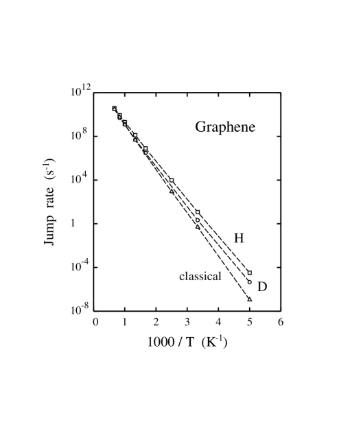
Figure 25: Rate for impurity jumps on a graphene sheet as a function of the inverse temperature. Symbols represent results derived from QTST for hydrogen (squares), deuterium (circles), and classical limit (triangles) Herrero and Ramírez (2009b). Dashed lines are guides to the eye.

In recent years, some simulations of adsorbed species on a single graphene layer have appeared in the literature. The chemisorption of atomic H and D on graphene was studied by PIMD simulations Herrero and Ramírez (2009b). Finite-temperature properties of these point defects were obtained by using a tight-binding potential fitted to DFT calculations. On one side, vibrational properties of the adatoms were studied at their equilibrium positions, linked to C atoms. The vibrations displayed an important anharmonicity, as derived from a comparison between the vibrational energy of hydrogen and deuterium. On the other side, motion of H and D was studied by QTST. For hydrogen, the diffusivity on the graphene sheet at 300 K turned out to be enhanced by quantum effects by a factor $\sim 20$, as can be seen in the Arrhenius-type plot of Fig. 25. QTST based on PIMC simulations has been also employed to study the diffusion of hydrogen on the Ni(100) surface Mattsson et al. (1993); Mattsson and Wahnström (1995, 1997).

More recently, the motion of hydrogen on the Ru(0001) surface between 75 and 250 K was studied in Ref. McIntosh et al. (2013) by a combination of ab initio PIMD simulations, QTST, and helium spin-echo measurements. Quantum effects were found to be significant at temperatures as high as 200 K, while for $T<$ 120 K a tunneling-dominated temperature-independent motion was observed, with a large jump rate of $\sim 10^{9}$ s^-1. The crossover to tunneling-dominated diffusion at low temperatures was well reproduced by the QTST calculations, but the tunneling rate turned out to be underestimated when compared with experimental data McIntosh et al. (2013).

Even though superfluidity in bulk molecular hydrogen has not been observed, reduction of dimensionality has been regarded as a possible way for the detection of a superfluid phase at low temperatures. This has motivated experimental and theoretical investigation of adsorbed films of para-H₂ on several substrates. With this question in mind, the low-temperature phase diagram of an ideal 2D sheet of para-H₂ was studied by Boninsegni Boninsegni (2004) from PIMC simulations. For $T\to 0$, the system was found to be a crystal at equilibrium, with a triangular lattice structure. No metastable liquid phase has been observed, and the system remained as a solid down to its spinodal density, breaking into solid clusters at lower densities. The equilibrium crystal was found to melt at $T\sim$ 7 K. A more realistic system was later studied by considering a 2D sheet of para-H₂ embedded in a crystalline matrix of alkali atoms Boninsegni (2005). For this system, the thermodynamically stable phase at $T\lesssim$ 5 K was a solid, commensurate with the underlying lattice. For simulated systems of small size, a nonzero superfluid signal for para-H₂ was observed, but results for larger system sizes were consistent with the absence of superfluidity in the thermodynamic limit.

In connection with the behavior of 2D H₂ films, and turning to three-dimensional solid hydrogen, an interesting question is the melting of the H₂ layers close to the surface, which is expected to happen at temperatures lower than the bulk melting. This was studied by Wagner and Ceperley Wagner and Ceperley (1996) using PIMC, who obtained density profiles perpendicular and parallel to the surface, and showed the formation of a liquid adlayer at 6 K, less than half the bulk melting temperature of para-H₂. The onset temperature and depth of H₂ surface melting was estimated by calculating the static structure factor for the individual H₂ layers, and no crystalline order was found down to 3 K in a partially filled H₂ adlayer at the free surface. Zero-point motion of H₂ molecules at the surface turned out to be larger than in the bulk, so that quantum effects largely amplify the melting point depression at the surface.

Adsorption of noble gases on a variety of solid surfaces and confined geometries has been also studied by using path-integral methods. Several works have been focused on ⁴He. In this respect, helium adsorption on graphene was studied by PIMC calculations using effective interatomic potentials Kwon and Ceperley (2012). The first ⁴He layer was found to be commensurate with the substrate, displaying a $C_{1/3}$ structure. Vacancy states in this structure were found to behave differently depending on the employed interaction potential. This means that they may appear as a cluster of localized vacancies or as mobile vacancies inducing finite superfluid fractions. For the second helium layer, exchange among ⁴He adatoms resulted in quantum melting of a $C_{7/12}$ commensurate structure. In a similar work, the adsorption of ⁴He on a lithium substrate at low temperature was studied by Boninsegni et al. Boninsegni et al. (1999). These authors employed PIMC simulations with an effective interatomic potential, as well as DFT calculations. Evidence for continuous growth of a ⁴He film was presented, with the appearance of a superfluid monolayer at low coverage and no well-defined layering at higher coverages. The coverage dependence of the estimated superfluid transition temperatures was found to be similar to the experimental one.

PIMC simulations have been also employed to determine the phase diagram of an isolated ⁴He film in a range of temperatures and coverages where it undergoes solidification, superfluidity, and a liquid-gas transition Gordillo and Ceperley (1998). The phase-transition densities were calculated, as well as the coefficients for a functional form of the free energy for the different phases. The resulting phase diagram turned out to be similar to that derived from experimental measurements of a second layer of helium on graphite. Furthermore, the superfluidity of grain boundaries in solid ⁴He has been studied by PIMC simulations based on a continuous-space worm algorithm Pollet et al. (2007). These boundaries are generically superfluid at low $T$, with a transition temperature of $\sim$ 0.5 K at the melting pressure. Superfluid grain boundaries were found far from the melting line, and a grain boundary in contact with the superfluid liquid at the melting curve was found to be mechanically stable.

In addition to these contributions to the study of ⁴He in low-dimensional geometries, several PI works have been devoted to heavier noble gases in confined spaces. Thus, neon adsorbed in the interstitial channels of a bundle of carbon nanotubes was studied using PIMC calculations Gordillo et al. (2004). The chemical potential of Ne atoms could be evaluated, allowing for an estimation of the temperature and pressure conditions for neon adsorption to take place in those channels. In connection with this, phase transitions and quantum effects in condensates of Lennard-Jones particles inside cylindrical pores were also discussed from PIMC results Hoffmann and Nielaba (2003). Several properties of this system were analyzed, such as the effects of pore diameter and adsorbate–particle interaction strength on the emerging structures and location of phase boundaries. For strong wall–particle interactions, qualitative agreement was found with experimental results for the freezing of Ar–pore condensates, while for lighter Ne-like particles, quantum delocalization effects gave rise to unexpected condensate structures. As a result of these simulations, it was concluded that nuclear quantum effects can change the freezing temperature by an amount as large as a 10% Hoffmann and Nielaba (2003).

In the context of surface science, PIMC techniques have been also applied to study model adsorbates with internal quantum states. Marx et al. Marx et al. (1993c) considered an adsorbate in the strong-binding and small-corrugation limit. In this case, the resulting 2D fluid was treated in the adiabatic approximation: particle translations were treated classically, whereas the internal degrees of freedom were modeled by interacting two-state tunneling systems. With these conditions, the temperature-coverage phase diagram was obtained by combining PIMC simulations with finite-size scaling. In spite of its simplicity, this adsorbate model presents a surprisingly complex phase diagram, including gas, liquid, and solid phases, as well as first- and second-order transitions Marx et al. (1993c). It is remarkable the detection of a square-lattice solid phase in coexistence with a gas phase at low temperatures.

Alfe and Gillan have recently employed path-integral simulations in combination with ab initio DFT calculations to construct practical techniques for computing the chemical potential of molecules adsorbed on surfaces, with full inclusion of nuclear quantum effects Alfe and Gillan (2010). These authors presented practical calculations for the case of H₂O on the MgO (001) surface at low coverage. It was shown that the number of time slices required in the PI discretization for the higher vibrational frequencies of the H₂O molecule can be strongly reduced by employing a thermodynamic integration with respect to the number of beads. The correctness of their path-integral results was demonstrated by calculations on a set of simple model systems, for which quantum contributions to the free energy can be exactly obtained from analytic arguments.

VIII Summary and outlook

The path-integral formulation of quantum mechanics has rendered it possible to theoretically tackle many problems that require the use of statistical mechanics with full consideration of quantum effects. The quantum-classical isomorphism derived for the statistical partition function allows the application of efficient classical simulation techniques, such as MC or MD, to the quantum domain. PI simulations reproduce quantum effects related to tunneling and anharmonic zero-point motion of atoms in solids, as well as other properties associated to the indistinguishability of the atomic nuclei. In this respect, the treatment of bosonic degrees of freedom has been proven to be feasible, while the consideration of fermionic systems remains in general as a challenging task. Also, the path-integral simulation of dynamic properties, such as time correlation functions, poses a challenge that at present can only be treated by approximate algorithms.

The fast increase in computing facilities, and in particular the use of parallel computers, opens new routes for PI simulations, both in terms of the kind of system and properties to be studied, as well as in terms of the computational methods. Limitations associated to the use of empirical potentials are currently being removed by the application of ab initio electronic structure methods. The appealing ‘all-quantum’ approach, combining the PI simulation of atomic nuclei with an ab initio DFT description of the electrons is, however, not free of shortcomings. For example, the DFT treatment of condensed phases of water has revealed to be elusive in reproducing certain thermodynamic properties, so that the development of new improved functionals is an active area of research.

This kind of quantum simulations are necessary to reproduce some observable properties of solids, that are not correctly described by classical simulations. Thus, PI simulation is an efficient tool to understand various isotope effects in solids, that at low temperature are a consequence of the anharmonicity of atomic zero-point vibrations. These effects are readily explored, since the atomic masses appear as input parameters in the PI calculations. This type of simulations enable one to obtain separately kinetic and potential energies at finite temperatures, taking into account the quantization of nuclear motion. This includes consideration of zero-point motion of the atoms in the solid, which can be hard to study by analytical approaches in the presence of light atoms and large anharmonicities. In this context, a good check of interatomic potentials is the calculation of macroscopic observables such as the molar volume, thermal expansion, bulk modulus, or heat capacity, which can be directly compared with experimental data. In addition, differences between PI and classical calculations can be used to assess the importance of quantum effects in the equilibrium properties of a given substance.

In this topical review, we have presented PI simulations of different types of solids. Noble-gas solids have allowed to check the methods and their application to obtain structural and thermodynamic properties, due to the relative simplicity of the interatomic potentials, as compared to solids including covalent or hydrogen bonds. Further applications of PI simulations have been concentrated on group-IV materials (mainly diamond, and the semiconductors Si, Ge, and SiC), for which the relevance of quantum effects in the presence of anharmonicity has been shown. Molecular solids have been also reviewed, with especial emphasis on hydrogen and ice, which have revealed important nuclear quantum effects. Another field of interest for PI simulations has been the diffusion of impurities in the bulk and adsorbates on the surface of various types of solids, a problem for which QTST has turned out to be very efficient.

PI simulations of amorphous helium, silicon, and ice have been also discussed. In a similar manner, this kind of simulations can yield information on the atom delocalization and anharmonic effects in other amorphous materials. In particular, this method may provide relevant information on H-containing amorphous solids, whose macroscopic properties can be affected by the quantum delocalization of hydrogen. Moreover, simulations in the context of QTST can give relevant information on the low-energy tunneling states that control the acoustic, thermal, and dielectric properties of amorphous materials at low temperatures.

Hydrogen is of particular interest for PI simulations, as has been shown along this topical review. The lowest atomic mass implies the prevalence of quantum effects related to it. The presence of hydrogen in molecules essential for biological systems means that classical simulations may be not accurate enough to reproduce some of their properties. Thus, quantum tunneling of protons is supposed to play a relevant role in some biological processes, affecting for example the mechanisms for enzyme reactivity and oxidation of monoamine neurotransmitters. In this line, we expect that the PI approach will reveal in the near future its capability in the investigation of quantum effects in biological systems, as has happened in the past for inorganic materials.

Appendix A Free particle density operator

Computer simulations based on the PIMD and PIMC methods rely on a discretized algorithm to approximate the temperature dependence of the exponential density operator, $e^{-\beta\widehat{H}}$. In this section we rationalize the basic steps of this algorithm by considering first an arbitrary function of the inverse temperature $f(\beta)$. One wants to approximate the evolution of $f$ starting at some initial value $\beta_{1}$. The Taylor expansion of $f$ can be written as

$$f(\beta_{1}+\beta)={\displaystyle\sum_{n=0}^{\infty}\frac{1}{n!}\left(\beta\frac{d}{d\beta}\right)}^{n}f(\beta_{1})\;.$$ (68)

Here we use the convention of expressing the $n$’th order differential operator as a power

$$\left(\frac{d}{d\beta}\right)^{n}f(\beta_{1})\equiv\left[\frac{d^{n}f(\beta)}{d\beta^{n}}\right]_{\beta=\beta_{1}}.$$ (69)

By considering a series expansion of the exponential function

$$e^{\beta}=\sum_{n=0}^{\infty}\frac{\beta^{n}}{n!}\;,$$ (70)

one obtains from Eq. (68) an alternative operator expression for the Taylor series

$$f(\beta_{1}+\beta)=\exp\left(\beta\frac{d}{d\beta}\right)f(\beta_{1})\;.$$ (71)

We refer to this exponential operator, $\exp\left(\beta\frac{d}{d\beta}\right)$, as an evolution operator. In our context, the first step of a discretized algorithm is the exact factorization of the evolution operator into $L$ factors

$$f(\beta_{1}+\beta)=\left[\exp\left(\frac{\beta}{L}\>\frac{d}{d\beta}\right)\right]^{L}f(\beta_{1})\;.$$ (72)

This factorization implies the discretization of $\beta$ into $L+1$ points separated by a small interval $\epsilon=\beta/L$. The next and most important step is the formulation of a high-temperature approximation for the evolution along the interval $\epsilon$. Note that a small $\epsilon$ is equivalent to a high temperature $TL$, as $\epsilon^{-1}=k_{B}TL$. The HTA is in general dependent on the problem under consideration. One simple alternative is the first term of the Taylor series

$$f(\beta_{1}+\epsilon)\equiv\left[\exp\left(\epsilon\>\frac{d}{d\beta}\right)\right]f(\beta_{1})\approx f(\beta_{1})+\epsilon\left[\frac{d\,f(\beta)}{d\beta}\right]_{\beta=\beta_{1}}\;.$$ (73)

Once a HTA is computer coded, the whole temperature dependence of $f(\beta)$ is obtained by a simple repeating loop that recalculates Eq. (73 ) for the successive $\epsilon$ intervals.

As a simple example let us apply a discretized algorithm to approximate the density matrix of a free particle. We denote the canonical density matrix for a free particle in one-dimension as $\rho(x,x^{\prime};\beta)$. Knowing that the high-temperature limit $(\beta\rightarrow 0)$ of $\rho$ is

$$\rho(x,x^{\prime};0)=\delta(x-x^{\prime})\;,$$ (74)

we aim to derive $\rho(x,x^{\prime};\beta)$ by a discretization of $\beta$ into steps $\epsilon=\beta/L$. We employ the HTA of Eq. (73),

$$\rho(x,x^{\prime};\epsilon)\approx\rho(x,x^{\prime};0)+\epsilon\left(\frac{\partial\rho(x,x^{\prime};\beta)}{\partial\beta}\right)_{\beta=0}\;.$$ (75)

The $\beta$ derivative is evaluated with the Bloch equation

$$\frac{\partial\rho(x,x^{\prime};\beta)}{\partial\beta}=-\widehat{H}\rho(x,x^{\prime};\beta)\;,\quad\mathrm{with}\quad\widehat{H}=-\frac{\hbar^{2}}{2m}\,\frac{\partial^{2}}{\partial x^{2}}\;.$$ (76)

Using the following representation of the delta function

$$\delta(x,x^{\prime})=\frac{1}{2\pi\hbar}\intop_{-\infty}^{\infty}dp\>e^{-ip(x-x^{\prime})/\hbar}\;,$$ (77)

the first derivative of $\rho(x,x^{\prime};\beta)$ at $\beta=0$ is obtained from Eqs. (74) and (76) as

$$-\widehat{H}\rho(x,x^{\prime};0)=\frac{1}{2\pi\hbar}\intop_{-\infty}^{\infty}dp\>\left(-\frac{p\text{\texttwosuperior}}{2m}\right)e^{-ip(x-x^{\prime})/\hbar}\;.$$ (78)

With the help of the previous equation, the HTA of $\rho(x,x^{\prime};\epsilon)$ in Eq. (75) becomes

$$\rho(x,x^{\prime};\epsilon)\approx\frac{1}{2\pi\hbar}\intop_{-\infty}^{\infty}dp\>\left(1-\frac{\epsilon p^{2}}{2m}\right)e^{-ip(x-x^{\prime})/\hbar}\;.$$ (79)

A straightforward repeating loop of the previous step gives the approximate density matrix for the discretized inverse temperatures $2\epsilon,3\epsilon,\ldots$. The final result for $L\epsilon=\beta$ is obtained by induction as

$$\rho(x,x^{\prime};\beta)\approx\frac{1}{2\pi\hbar}\intop_{-\infty}^{\infty}dp\>\left(1-\frac{\epsilon p^{2}}{2m}\right)^{L}e^{-ip(x-x^{\prime})/\hbar}\;.$$ (80)

The error of this discretized approximation vanishes in the limit $L\rightarrow\infty$. One can check it by substitution of $\epsilon=\beta/L$, and by considering the definition of the exponential function

$$e^{-x}=\lim_{L\rightarrow\infty}\left(1-\frac{x}{L}\right)^{L}\;.$$ (81)

Thus, in the limit $L\rightarrow\infty$

$$\rho(x,x^{\prime};\beta)=\frac{1}{2\pi\hbar}\intop_{-\infty}^{\infty}dp\>e^{-\beta p^{2}/2m}\,e^{-ip(x-x^{\prime})/\hbar}\;.$$ (82)

This Gaussian integration is analytic, providing the final exact free particle result Feynman (1972)

$$\rho(x,x^{\prime};\beta)=\left(\frac{m}{2\pi\beta\hbar^{2}}\right)^{1/2}e^{-m(x-x^{\prime})^{2}/2\beta\hbar^{2}}\;.$$ (83)

References

- Ceperley and Alder (1986) D. M. Ceperley and B. Alder, Science 231, 555 (1986).
- Marx and Muser (1999) D. Marx and M. Muser, J. Phys.: Condens. Matter 11, R117 (1999).
- Feynman (1948) R. P. Feynman, Rev. Mod. Phys. 20, 367 (1948).
- Chandler and Wolynes (1981) D. Chandler and P. G. Wolynes, J. Chem. Phys. 74, 4078 (1981).
- Morita (1973) T. Morita, J. Phys. Soc. Jap. 35, 980 (1973).
- Balker (1979) J. Balker, J. Chem. Phys. 70, 2914 (1979).
- Berne and Thirumalai (1986) B. J. Berne and D. Thirumalai, Annu. Rev. Phys. Chem. 37, 401 (1986).
- Gillan (1990) M. J. Gillan, in Computer Modelling of Fluids, Polymers and Solids, edited by C. R. A. Catlow, S. C. Parker, and M. P. Allen (Kluwer, Dordrecht, 1990), p. 155.
- Ceperley (1995) D. M. Ceperley, Rev. Mod. Phys. 67, 279 (1995).
- Chakravarty (1997) C. Chakravarty, Int. Rev. Phys. Chem. 16, 421 (1997).
- Tuckerman and Hughes (1998) M. E. Tuckerman and A. Hughes, in Classical and Quantum Dynamics in Condensed Phase Simulations, edited by B. J. Berne, G. Ciccotti, and D. F. Coker (Word Scientific, Singapore, 1998), p. 311.
- Feynman and Hibbs (1965) R. P. Feynman and A. R. Hibbs, Quantum Mechanics and Path Integrals (McGraw-Hill, New York, 1965).
- Feynman (1972) R. P. Feynman, Statistical Mechanics (Addison-Wesley, New York, 1972).
- Kleinert (1990) H. Kleinert, Path Integrals in Quantum Mechanics, Statistics and Polymer Physics (World Scientific, Singapore, 1990).
- Tuckerman (2010) M. E. Tuckerman, Statistical Mechanics: Theory and Molecular Simulation (Oxford University Press, New York, 2010).
- Gillan (1988) M. J. Gillan, Phil. Mag. A 58, 257 (1988).
- Marx and Hutter (2009) D. Marx and J. Hutter, Ab initio Molecular Mechanics: Basic Theory and Advanced Methods (Cambridge University Press, Cambridge, 2009).
- Buschert et al. (1988) R. C. Buschert, A. E. Merlini, S. Pace, S. Rodriguez, and M. H. Grimsditch, Phys. Rev. B 38, 5219 (1988).
- Holloway et al. (1991) H. Holloway, K. C. Hass, M. A. Tamor, T. R. Anthony, and W. F. Banholzer, Phys. Rev. B 44, 7123 (1991).
- Noya et al. (1997a) J. C. Noya, C. P. Herrero, and R. Ramírez, Phys. Rev. B 56, 237 (1997a).
- Herrero (1999) C. P. Herrero, Solid State Commun. 110, 243 (1999).
- Herrero et al. (2009) C. P. Herrero, R. Ramírez, and M. Cardona, Phys. Rev. B 79, 012301 (2009).
- Berne (1986) B. J. Berne, J. Stat. Phys. 43, 911 (1986).
- Hone et al. (2006) T. D. Hone, P. J. Rossky, and G. A. Voth, J. Chem. Phys. 124, 154103 (2006).
- Pérez et al. (2009) A. Pérez, M. E. Tuckerman, and M. H. Müser, J. Chem. Phys. 130, 184105 (2009).
- Habershon et al. (2013) S. Habershon, D. E. Manolopoulos, T. E. Markland, and T. F. Miller, Annu. Rev. Phys. Chem. 64, 387 (2013).
- Hirsch et al. (1982) J. E. Hirsch, R. L. Sugar, D. J. Scalapino, and R. Blankenbecler, Phys. Rev. B 26, 5033 (1982).
- De Raedt and Lagendijk (1985) H. De Raedt and A. Lagendijk, Phys. Rep. 127, 233 (1985).
- Von Der Linden (1992) W. Von Der Linden, Phys. Rep. 220, 53 (1992).
- Batrouni and Scalettar (1992) G. G. Batrouni and R. T. Scalettar, Phys. Rev. B 46, 9051 (1992).
- Foulkes et al. (2001) W. M. C. Foulkes, L. Mitas, R. J. Needs, and G. Rajagopal, Rev. Mod. Phys. 73, 33 (2001).
- Needs et al. (2010) R. J. Needs, M. D. Towler, N. D. Drummond, and P. L. Rios, J. Phys.: Condens. Matter 22, 023201 (2010).
- Gull et al. (2011) E. Gull, A. J. Millis, A. I. Lichtenstein, A. N. Rubtsov, M. Troyer, and P. Werner, Rev. Mod. Phys. 83, 349 (2011).
- Schulman (1981) L. S. Schulman, Techniques and Applications of Path Integration (Wiley, New York, 1981).
- Takahashi and Imada (1984) M. Takahashi and M. Imada, J. Phys. Soc. Jap. 53, 3765 (1984).
- Parrinello and Rahman (1980) M. Parrinello and A. Rahman, Phys. Rev. Lett. 45, 1196 (1980).
- Parrinello and Rahman (1981) M. Parrinello and A. Rahman, J. Appl. Phys. 52, 7182 (1981).
- Souza and Martins (1997) I. Souza and J. L. Martins, Phys. Rev. B 55, 8733 (1997).
- Frenkel and Smit (1996) D. Frenkel and B. Smit, Understanding Molecular Simulation (Academic Press, San Diego, 1996).
- Freeman and Doll (1984) D. L. Freeman and J. D. Doll, J. Chem. Phys. 80, 5709 (1984).
- Coalson (1986) R. D. Coalson, J. Chem. Phys. 85, 926 (1986).
- Chakravarty et al. (1998) C. Chakravarty, M. C. Gordillo, and D. M. Ceperley, J. Chem. Phys. 109, 2123 (1998).
- Vorontsov-Velyaminov et al. (1997) P. N. Vorontsov-Velyaminov, M. O. Nesvit, and R. I. Gorbunov, Phys. Rev. E 55, 1979 (1997).
- Herman et al. (1982) M. F. Herman, E. J. Bruskin, and B. J. Berne, J. Chem. Phys. 76, 5150 (1982).
- Parrinello and Rahman (1984) M. Parrinello and A. Rahman, J. Chem. Phys. 80, 860 (1984).
- Sesé (2003) L. M. Sesé, Mol. Phys. 101, 1455 (2003).
- Martyna et al. (1996) G. J. Martyna, M. E. Tuckerman, D. J. Tobias, and M. L. Klein, Mol. Phys. 87, 1117 (1996).
- Martyna et al. (1999) G. J. Martyna, A. Hughes, and M. E. Tuckerman, J. Chem. Phys. 110, 3275 (1999).
- Tuckerman (2002) M. E. Tuckerman, in Quantum Simulations of Complex Many–Body Systems: From Theory to Algorithms, edited by J. Grotendorst, D. Marx, and A. Muramatsu (NIC, FZ Jülich, 2002), p. 269.
- Tuckerman et al. (1993) M. E. Tuckerman, B. J. Berne, G. J. Martyna, and M. L. Klein, J. Chem. Phys. 99, 2796 (1993).
- Martyna and Klein (1992) G. J. Martyna and M. L. Klein, J. Chem. Phys. 97, 2635 (1992).
- Tuckerman et al. (2006) M. E. Tuckerman, J. Alejandre, R. López-Rendón, A. L. Jochim, and G. J. Martyna, J. Phys. A: Math. Gen. 39, 5629 (2006).
- Tuckerman et al. (1992) M. E. Tuckerman, B. J. Berne, and G. J. Martyna, J. Chem. Phys. 97, 1990 (1992).
- Johnson et al. (1993) J. K. Johnson, J. A. Zollweg, and K. E. Gubbins, Mol. Phys. 78, 591 (1993).
- (55) The number of cell degrees of freedom is important because it appears as a force factor in the equation of motion related to the first barostat that is coupled to the volume. In the original literature this force term is given as , where is the spatial dimension [see Eq. (D1) in Ref. Martyna et al., 1999]. We note that this term should be modified in the case that the rotation of the unit cell is eliminated, because the number of cell degrees of freedom is reduced from to . In this case the factor in the force of the first barostat should be changed to in order to generate the correct ensemble distribution.
- Gillan (1987a) M. J. Gillan, J. Phys. C: Solid State Phys. 20, 3621 (1987a).
- Cao and Voth (1994a) J. Cao and G. A. Voth, J. Chem. Phys. 100, 5093 (1994a).
- Cao and Voth (1994b) J. Cao and G. A. Voth, J. Chem. Phys. 100, 5106 (1994b).
- Jang and Voth (1999) S. Jang and G. A. Voth, J. Chem. Phys. 111, 2371 (1999).
- Craig and Manolopoulos (2004) I. R. Craig and D. E. Manolopoulos, J. Chem. Phys. 121, 3368 (2004).
- Ramírez and Herrero (2005) R. Ramírez and C. P. Herrero, Phys. Rev. B 72, 024303 (2005).
- Ramírez and López-Ciudad (2001) R. Ramírez and T. López-Ciudad, J. Chem. Phys. 115, 103 (2001).
- López-Ciudad et al. (2003) T. López-Ciudad, R. Ramírez, J. Schulte, and M. C. Böhm, J. Chem. Phys. 119, 4328 (2003).
- Ramírez and López-Ciudad (2002) R. Ramírez and T. López-Ciudad, in Quantum Simulations of Complex Many–Body Systems: From Theory to Algorithms, edited by J. Grotendorst, D. Marx, and A. Muramatsu (NIC, FZ Jülich, 2002), pp. 325–375.
- Kirkwood (1935) J. G. Kirkwood, J. Chem. Phys. 3, 300 (1935).
- Allen and Tildesley (1987) M. P. Allen and D. J. Tildesley, Computer Simulation of Liquids (Clarendon Press, Oxford, 1987).
- Frenkel and Ladd (1984) D. Frenkel and A. J. C. Ladd, J. Chem. Phys. 81, 3188 (1984).
- Polson et al. (2000) J. M. Polson, E. Trizac, S. Pronk, and D. Frenkel, J. Chem. Phys. 112, 5339 (2000).
- Morales and Singer (1991) J. J. Morales and K. Singer, Mol. Phys. 73, 873 (1991).
- Ramírez and Herrero (2010) R. Ramírez and C. P. Herrero, J. Chem. Phys. 133, 144511 (2010).
- Watanabe and Reinhardt (1990) M. Watanabe and W. P. Reinhardt, Phys. Rev. Lett. 65, 3301 (1990).
- Valle and Venuti (1998) R. G. D. Valle and E. Venuti, Phys. Rev. B 58, 206 (1998).
- Cuccoli et al. (1997) A. Cuccoli, A. Macchi, G. Pedrolli, V. Tognetti, and R. Vaia, Phys. Rev. B 56, 51 (1997).
- Cuccoli et al. (1993) A. Cuccoli, A. Macchi, V. Tognetti, and R. Vaia, Phys. Rev. B 47, 14923 (1993).
- Müser et al. (1995) M. H. Müser, P. Nielaba, and K. Binder, Phys. Rev. B 51, 2723 (1995).
- Thirumalai et al. (1984) D. Thirumalai, R. W. Hall, and B. J. Berne, J. Chem. Phys. 81, 2523 (1984).
- Herrero (2002) C. P. Herrero, Phys. Rev. B 65, 014112 (2002).
- Herrero (2003a) C. P. Herrero, J. Phys.: Condens. Matter 15, 475 (2003a).
- Aziz et al. (1995) R. A. Aziz, A. R. Janzen, and M. R. Moldover, Phys. Rev. Lett. 74, 1586 (1995).
- Timms et al. (1996) D. N. Timms, A. C. Evans, M. Boninsegni, D. M. Ceperley, J. Mayers, and R. O. Simmons, J. Phys.: Condens. Matter 8, 6665 (1996).
- Loubeyre (1987) P. Loubeyre, Phys. Rev. Lett. 58, 1857 (1987).
- Boninsegni et al. (1994) M. Boninsegni, C. Pierleoni, and D. M. Ceperley, Phys. Rev. Lett. 72, 1854 (1994).
- Chang and Boninsegni (2001) S. Y. Chang and M. Boninsegni, J. Chem. Phys. 115, 2629 (2001).
- Herrero (2006) C. P. Herrero, J. Phys.: Condens. Matter 18, 3469 (2006).
- Barrat et al. (1989) J. L. Barrat, P. Loubeyre, and M. L. Klein, J. Chem. Phys. 90, 5644 (1989).
- Draeger and Ceperley (2000) E. W. Draeger and D. M. Ceperley, Phys. Rev. B 61, 12094 (2000).
- Rota and Boronat (2011a) R. Rota and J. Boronat, J. Low Temp. Phys. 162, 146 (2011a).
- Ceperley et al. (1996) D. M. Ceperley, R. O. Simmons, and R. C. Blasdell, Phys. Rev. Lett. 77, 115 (1996).
- Mao et al. (1988) H. K. Mao, R. J. Hemley, Y. Wu, A. P. Jephcoat, L. W. Finger, C. S. Zha, and W. A. Bassett, Phys. Rev. Lett. 60, 2649 (1988).
- Loubeyre et al. (1993) P. Loubeyre, R. LeToullec, J. P. Pinceaux, H. K. Mao, J. Hu, and R. J. Hemley, Phys. Rev. Lett. 71, 2272 (1993).
- Herrero (2008) C. P. Herrero, J. Phys.: Condens. Matter 20, 295230 (2008).
- Rota and Boronat (2011b) R. Rota and J. Boronat, Mol. Phys. 109, 2963 (2011b).
- Candido et al. (2011) L. Candido, G. Q. Hai, and D. M. Ceperley, Phys. Rev. B 84, 064515 (2011).
- Boninsegni et al. (2006a) M. Boninsegni, N. Prokofév, and B. Svistunov, Phys. Rev. Lett. 96, 105301 (2006a).
- Kim and Chan (2004) E. Kim and M. H. W. Chan, Science 305, 1941 (2004).
- Kim and Chan (2012) D. Y. Kim and M. H. W. Chan, Phys. Rev. Lett. 109, 155301 (2012).
- Ceperley and Bernu (2004) D. M. Ceperley and B. Bernu, Phys. Rev. Lett. 93 (2004).
- Clark and Ceperley (2006) B. K. Clark and D. M. Ceperley, Phys. Rev. Lett. 96, 105302 (2006).
- Rota and Boronat (2012) R. Rota and J. Boronat, Phys. Rev. Lett. 108, 045308 (2012).
- Neumann and Zoppi (2000) M. Neumann and M. Zoppi, Phys. Rev. B 62, 41 (2000).
- Chakravarty (2002) C. Chakravarty, J. Chem. Phys. 116, 8938 (2002).
- Neumann and Zoppi (2002) M. Neumann and M. Zoppi, Phys. Rev. E 65, 031203 (2002).
- Giachetti and Tognetti (1986) R. Giachetti and V. Tognetti, Phys. Rev. B 33, 7647 (1986).
- Feynman and Kleinert (1986) R. P. Feynman and H. Kleinert, Phys. Rev. A 34, 5080 (1986).
- Cuccoli et al. (1992) A. Cuccoli, A. Macchi, M. Neumann, V. Tognetti, and R. Vaia, Phys. Rev. B 45, 2088 (1992).
- Acocella et al. (2000) D. Acocella, G. K. Horton, and E. R. Cowley, Phys. Rev. B 61, 8753 (2000).
- Acocella et al. (1995) D. Acocella, G. K. Horton, and E. R. Cowley, Phys. Rev. Lett. 74, 4887 (1995).
- Somoza and Fenichel (1971) E. Somoza and H. Fenichel, Phys. Rev. B 3, 3434 (1971).
- Fenichel and Serin (1966) H. Fenichel and B. Serin, Phys. Rev. 142, 490 (1966).
- Peterson et al. (1966) O. G. Peterson, D. N. Batchelder, and R. O. Simmons, Phys. Rev. 150, 703 (1966).
- Pollack (1964) G. L. Pollack, Rev. Mod. Phys. 36, 748 (1964).
- Granfors et al. (1981) P. R. Granfors, A. T. Macrander, and R. O. Simmons, Phys. Rev. B 24, 4753 (1981).
- Losee and Simmons (1968) D. L. Losee and R. O. Simmons, Phys. Rev. 172, 944 (1968).
- Chakravarty (2011) C. Chakravarty, J. Phys. Chem. A 115, 7028 (2011).
- Herrero and Ramírez (2005) C. P. Herrero and R. Ramírez, Phys. Rev. B 71, 174111 (2005).
- Endoh et al. (1975) Y. Endoh, G. Shirane, and J. Skalyo, Jr., Phys. Rev. B 11, 1681 (1975).
- McLaren et al. (1975) R. A. McLaren, H. Kiefte, D. Landheer, and B. P. Stoicheff, Phys. Rev. B 11, 1705 (1975).
- Shimizu et al. (2001) H. Shimizu, H. Tashiro, T. Kume, and S. Sasaki, Phys. Rev. Lett. 86, 4568 (2001).
- Schöffel and Müser (2001) P. Schöffel and M. H. Müser, Phys. Rev. B 63, 224108 (2001).
- Herrero (2003b) C. P. Herrero, Phys. Rev. B 68, 172104 (2003b).
- Ramírez and Herrero (2008) R. Ramírez and C. P. Herrero, J. Chem. Phys. 129, 204502 (2008).
- Ramírez et al. (2008a) R. Ramírez, C. P. Herrero, A. Antonelli, and E. R. Hernández, J. Chem. Phys. 129, 064110 (2008a).
- Brito and Antonelli (2012) B. G. A. Brito and A. Antonelli, J. Chem. Phys. 137, 034114 (2012).
- de Koning et al. (1999) M. de Koning, A. Antonelli, and S. Yip, Phys. Rev. Lett. 83, 3973 (1999).
- Sesé (2013) L. M. Sesé, J. Chem. Phys. 139, 044502 (2013).
- Ramírez and Herrero (1993) R. Ramírez and C. P. Herrero, Phys. Rev. B 48, 14659 (1993).
- Noya et al. (1996) J. C. Noya, C. P. Herrero, and R. Ramírez, Phys. Rev. B 53, 9869 (1996).
- Madelung (1982) O. Madelung, ed., Physics of Group IV Elements and III-V Compounds, vol. 17a of Landolt-Börnstein, New Series Group III (Springer-Verlag, Berlin, 1982).
- Hall (1961) R. O. A. Hall, Acta Crystallogr. 14, 1004 (1961).
- Shah and Straumanis (1972) J. S. Shah and M. E. Straumanis, Solid State Commun. 10, 159 (1972).
- Gerlich et al. (1965) D. Gerlich, B. Abeles, and R. E. Miller, J. Appl. Phys. 36, 76 (1965).
- Shanks et al. (1963) H. R. Shanks, P. D. Maycock, P. H. Sidles, and G. C. Danielson, Phys. Rev. 130, 1743 (1963).
- Pavone and Baroni (1994) P. Pavone and S. Baroni, Solid State Commun. 90, 295 (1994).
- Baroni et al. (2001) S. Baroni, S. de Gironcoli, and A. D. Corso, Rev. Mod. Phys. 73, 515 (2001).
- Herrero (1998) C. P. Herrero, Europhys. Lett. 44, 734 (1998).
- Müser (2001) M. H. Müser, J. Chem. Phys. 114, 6364 (2001).
- Rickwardt et al. (2001) C. Rickwardt, P. Nielaba, M. H. Muser, and K. Binder, Phys. Rev. B 63, 045204 (2001).
- Tersoff (1988) J. Tersoff, Phys. Rev. Lett. 61, 2879 (1988).
- Herrero and Ramírez (2001) C. P. Herrero and R. Ramírez, Phys. Rev. B 63, 024103 (2001).
- Ramírez et al. (2006) R. Ramírez, C. P. Herrero, and E. R. Hernández, Phys. Rev. B 73, 245202 (2006).
- Zollner et al. (1992) S. Zollner, M. Cardona, and S. Gopalan, Phys. Rev. B 45, 3376 (1992).
- Herchen and Cappelli (1991) H. Herchen and M. A. Cappelli, Phys. Rev. B 43, 11740 (1991).
- Zouboulis et al. (1998) E. S. Zouboulis, M. Grimsditch, A. K. Ramdas, and S. Rodriguez, Phys. Rev. B 57, 2889 (1998).
- Ceriotti et al. (2009) M. Ceriotti, G. Bussi, and M. Parrinello, Phys. Rev. Lett. 103, 030603 (2009).
- Ramírez et al. (2008b) R. Ramírez, C. P. Herrero, E. R. Hernández, and M. Cardona, Phys. Rev. B 77, 045210 (2008b).
- McMahon et al. (2012) J. M. McMahon, M. A. Morales, C. Pierleoni, and D. M. Ceperley, Rev. Mod. Phys. 84, 1607 (2012).
- Zoppi and Neumann (1991) M. Zoppi and M. Neumann, Phys. Rev. B 43, 10242 (1991).
- Cui et al. (1997) T. Cui, E. Cheng, B. J. Alder, and K. B. Whaley, Phys. Rev. B 55, 12253 (1997).
- Cui et al. (2001) T. Cui, Y. Takada, Q. Cui, Y. Ma, and G. Zou, Phys. Rev. B 64, 024108 (2001).
- Cui et al. (2002) T. Cui, Y. Ma, and G. Zou, J. Phys.: Condens. Matter 14, 10901 (2002).
- Biermann et al. (1998) S. Biermann, D. Hohl, and D. Marx, Solid State Commun. 108, 337 (1998).
- Kitamura et al. (2000) H. Kitamura, S. Tsuneyuki, T. Ogitsu, and T. Miyake, Nature 404, 259 (2000).
- Tsuneyuki et al. (2001) S. Tsuneyuki, H. Kitamura, T. Ogitsu, and T. Miyake, J. Low Temp. Phys. 122, 291 (2001).
- Geneste et al. (2012) G. Geneste, M. Torrent, F. Bottin, and P. Loubeyre, Phys. Rev. Lett. 109, 155303 (2012).
- Li et al. (2013) X.-Z. Li, B. Walker, M. I. J. Probert, C. J. Pickard, R. J. Needs, and A. Michaelides, J. Phys.: Condens. Matter 25, 085402 (2013).
- Howie et al. (2012) R. T. Howie, C. L. Guillaume, T. Scheler, A. F. Goncharov, and E. Gregoryanz, Phys. Rev. Lett. 108, 125501 (2012).
- Surh et al. (1997) M. P. Surh, K. J. Runge, T. W. Barbee, E. L. Pollock, and C. Mailhiot, Phys. Rev. B 55, 11330 (1997).
- Kaxiras and Guo (1994) E. Kaxiras and Z. Guo, Phys. Rev. B 49, 11822 (1994).
- Runge et al. (1992) K. J. Runge, M. P. Surh, C. Mailhiot, and E. L. Pollock, Phys. Rev. Lett. 69, 3527 (1992).
- Barker and Watts (1969) J. A. Barker and R. O. Watts, Chem. Phys. Lett. 3, 144 (1969).
- Rahman and Stillinger (1971) A. Rahman and F. H. Stillinger, J. Chem. Phys. 55, 3336 (1971).
- Gai et al. (1996a) H. Gai, G. K. Schenter, and B. C. Garrett, J. Chem. Phys. 104, 680 (1996a).
- Hernández de la Peña et al. (2005) L. Hernández de la Peña, M. S. Gulam Razul, and P. G. Kusalik, J. Chem. Phys. 123, 144506 (2005).
- Hernández de la Peña and Kusalik (2006) L. Hernández de la Peña and P. G. Kusalik, J. Chem. Phys. 125, 054512 (2006).
- Paesani and Voth (2008) F. Paesani and G. A. Voth, J. Phys. Chem. C 112, 324 (2008).
- McBride et al. (2009) C. McBride, C. Vega, E. G. Noya, R. Ramírez, and L. M. Sesé, J. Chem. Phys. 131, 024506 (2009).
- Koyama et al. (2004) Y. Koyama, H. Tanaka, G. Gao, and X. C. Zeng, J. Chem. Phys. 121, 7926 (2004).
- Jorgensen and Tirado-Rives (2005) W. L. Jorgensen and J. Tirado-Rives, Proc. Natl. Acad. Sci. USA 102, 6665 (2005).
- Abascal and Vega (2005) J. L. F. Abascal and C. Vega, J. Chem. Phys. 123, 234505 (2005).
- Paesani et al. (2006) F. Paesani, W. Zhang, D. A. Case, T. E. Cheatham, and G. A. Voth, J. Chem. Phys. 125, 184507 (2006).
- Habershon et al. (2009) S. Habershon, T. E. Markland, and D. E. Manolopoulos, J. Chem. Phys. 131, 024501 (2009).
- Mahoney and Jorgensen (2001) M. W. Mahoney and W. L. Jorgensen, J. Chem. Phys. 115, 10758 (2001).
- Fernández-Serra and Artacho (2006) M. V. Fernández-Serra and E. Artacho, Phys. Rev. Lett. 96, 016404 (2006).
- Morrone and Car (2008) J. A. Morrone and R. Car, Phys. Rev. Lett. 101, 017801 (2008).
- Li et al. (2011) X.-Z. Li, B. Walker, and A. Michaelides, Proc. Nat. Acad. Sci. USA 108, 6369 (2011).
- Kong et al. (2012) L. Kong, X. Wu, and R. Car, Phys. Rev. B 86, 134203 (2012).
- Yoo et al. (2009) S. Yoo, X. C. Zeng, and S. S. Xantheas, J. Chem. Phys. 130, 221102 (2009).
- Corsetti et al. (2013) F. Corsetti, E. Artacho, J. M. Soler, S. S. Alexandre, and M. V. Fernández-Serra, J. Chem. Phys. 139, 194502 (2013).
- Vega et al. (2010) C. Vega, M. M. Conde, C. McBride, J. L. F. Abascal, E. G. Noya, R. Ramírez, and L. M. Sesé, J. Chem. Phys. 132, 046101 (2010).
- McBride et al. (2012) C. McBride, E. G. Noya, J. L. Aragones, M. M. Conde, and C. Vega, Phys. Chem. Chem. Phys. 14, 10140 (2012).
- Conde et al. (2010) M. M. Conde, C. Vega, C. McBride, E. G. Noya, R. Ramírez, and L. M. Sesé, J. Chem. Phys. 132, 114503 (2010).
- Herrero and Ramírez (2011) C. P. Herrero and R. Ramírez, J. Chem. Phys. 134, 094510 (2011).
- Röttger et al. (1994) K. Röttger, A. Endriss, J. Ihringer, S. Doyle, and W. F. Kuhs, Acta Cryst. B 50, 644 (1994).
- Pamuk et al. (2012) B. Pamuk, J. M. Soler, R. Ramírez, C. P. Herrero, P. W. Stephens, P. B. Allen, and M. V. Fernández-Serra, Phys. Rev. Lett. 108, 193003 (2012).
- Ramírez and Herrero (2011) R. Ramírez and C. P. Herrero, Phys. Rev. B 84, 064130 (2011).
- Soper (2009) A. K. Soper, Phys. Rev. Lett. 103, 069801 (2009).
- Pietropaolo et al. (2009) A. Pietropaolo, R. Senesi, C. Andreani, A. Botti, M. A. Ricci, and F. Bruni, Phys. Rev. Lett. 103, 069802 (2009).
- Herrero and Ramírez (2011) C. P. Herrero and R. Ramírez, Phys. Rev. B 84, 224112 (2011).
- Mishima et al. (1984) O. Mishima, L. D. Calvert, and E. Whalley, Nature 310, 393 (1984).
- Sciortino et al. (1995) F. Sciortino, U. Essmann, H. E. Stanley, M. Hemmati, J. Shao, G. H. Wolf, and C. A. Angell, Phys. Rev. E 52, 6484 (1995).
- Strässle et al. (2004) T. Strässle, A. M. Saitta, S. Klotz, and M. Braden, Phys. Rev. Lett. 93, 225901 (2004).
- Herrero and Ramírez (2012) C. P. Herrero and R. Ramírez, J. Chem. Phys. 137, 104505 (2012).
- Gai et al. (1996b) H. Gai, G. K. Schenter, and B. C. Garrett, Phys. Rev. B 54, 14873 (1996b).
- Burnham et al. (2006) C. J. Burnham, G. F. Reiter, J. Mayers, T. Abdul-Redah, H. Reichert, and H. Dosch, Phys. Chem. Chem. Phys. 8, 3966 (2006).
- Burnham et al. (2008) C. J. Burnham, D. J. Anick, P. K. Mankoo, and G. F. Reiter, J. Chem. Phys. 128, 154519 (2008).
- Lin et al. (2011) L. Lin, J. A. Morrone, R. Car, and M. Parrinello, Phys. Rev. B 83, 220302 (2011).
- Benoit et al. (1998) M. Benoit, D. Marx, and M. Parrinello, Nature 392, 258 (1998).
- Benoit et al. (1999) M. Benoit, D. Marx, and M. Parrinello, Solid State Ionics 125, 23 (1999).
- Morrone et al. (2009) J. A. Morrone, L. Lin, and R. Car, J. Chem. Phys. 130, 204511 (2009).
- Presber et al. (1998) M. Presber, D. Loding, R. Martonak, and P. Nielaba, Phys. Rev. B 58, 11937 (1998).
- Müser and Berne (1996) M. H. Müser and B. J. Berne, Phys. Rev. Lett. 77, 2638 (1996).
- Rutledge et al. (1998) G. C. Rutledge, D. J. Lacks, R. Martonak, and K. Binder, J. Chem. Phys. 108, 10274 (1998).
- Martonak et al. (1998) R. Martonak, W. Paul, and K. Binder, Phys. Rev. E 57, 2425 (1998).
- Ramírez et al. (1997) R. Ramírez, C. P. Herrero, E. Artacho, and F. Ynduráin, J. Phys.: Condens. Matter 9, 3107 (1997).
- Krumrine et al. (2000) J. R. Krumrine, S. M. Jang, M. H. Alexander, and G. A. Voth, J. Chem. Phys. 113, 9079 (2000).
- Mirijanian et al. (2002) D. T. Mirijanian, M. H. Alexander, and G. A. Voth, Chem. Phys. Lett. 365, 487 (2002).
- Herrero and Ramírez (1995) C. P. Herrero and R. Ramírez, Phys. Rev. B 51, 16761 (1995).
- Ramírez and Herrero (1994) R. Ramírez and C. P. Herrero, Phys. Rev. Lett. 73, 126 (1994).
- Miyake et al. (1998) T. Miyake, T. Ogitsu, and S. Tsuneyuki, Phys. Rev. Lett. 81, 1873 (1998).
- Noya et al. (1997b) J. C. Noya, C. P. Herrero, and R. Ramírez, Phys. Rev. B 56, 15139 (1997b).
- Noya et al. (1997c) J. C. Noya, C. P. Herrero, and R. Ramírez, Phys. Rev. Lett. 79, 111 (1997c).
- Herrero et al. (2006) C. P. Herrero, R. Ramírez, and E. R. Hernández, Phys. Rev. B 73, 245211 (2006).
- Herrero and Ramírez (2009a) C. P. Herrero and R. Ramírez, Phys. Rev. B 80, 035207 (2009a).
- Herrero and Ramírez (2010) C. P. Herrero and R. Ramírez, Phys. Rev. B 82, 174117 (2010).
- Artacho et al. (1997) E. Artacho, F. Ynduráin, B. Pajot, R. Ramírez, C. P. Herrero, L. I. Khirunenko, K. M. Itoh, and E. E. Haller, Phys. Rev. B 56, 3820 (1997).
- Scharf et al. (1993) D. Scharf, G. J. Martyna, D. H. Li, G. A. Voth, and M. L. Klein, J. Chem. Phys. 99, 9013 (1993).
- Ma et al. (2001) Y. M. Ma, T. Cui, and G. T. Zou, J. Chem. Phys. 114, 3092 (2001).
- Clark and Ceperley (2008) B. K. Clark and D. M. Ceperley, Comp. Phys. Commun. 179, 82 (2008).
- Gillan (1987b) M. J. Gillan, Phys. Rev. Lett. 58, 563 (1987b).
- Herrero (1997) C. P. Herrero, Phys. Rev. B 55, 9235 (1997).
- Mattsson et al. (1993) T. R. Mattsson, U. Engberg, and G. Wahnström, Phys. Rev. Lett. 71, 2615 (1993).
- Forsythe and Makri (1998) K. M. Forsythe and N. Makri, J. Chem. Phys. 108, 6819 (1998).
- Herrero and Ramírez (2007) C. P. Herrero and R. Ramírez, Phys. Rev. Lett. 99, 205504 (2007).
- Jang and Voth (1998) S. J. Jang and G. A. Voth, J. Chem. Phys. 108, 4098 (1998).
- Boninsegni et al. (2006b) M. Boninsegni, A. B. Kuklov, L. Pollet, N. V. Prokofév, B. V. Svistunov, and M. Troyer, Phys. Rev. Lett. 97, 080401 (2006b).
- Markland et al. (2008) T. E. Markland, S. Habershon, and D. E. Manolopoulos, J. Chem. Phys. 128, 194506 (2008).
- Marx et al. (1993a) D. Marx, O. Opitz, P. Nielaba, and K. Binder, Phys. Rev. Lett. 70, 2908 (1993a).
- Marx et al. (1993b) D. Marx, S. Sengupta, and P. Nielaba, J. Chem. Phys. 99, 6031 (1993b).
- Nho and Manousakis (2002) K. Nho and E. Manousakis, Phys. Rev. B 65, 115409 (2002).
- Turnbull and Boninsegni (2007) J. Turnbull and M. Boninsegni, Phys. Rev. B 76, 104524 (2007).
- Marx et al. (1994) D. Marx, S. Sengupta, P. Nielaba, and K. Binder, Phys. Rev. Lett. 72, 262 (1994).
- Li et al. (2010) X.-Z. Li, M. I. J. Probert, A. Alavi, and A. Michaelides, Phys. Rev. Lett. 104, 066102 (2010).
- Herrero and Ramírez (2009b) C. P. Herrero and R. Ramírez, Phys. Rev. B 79, 115429 (2009b).
- Mattsson and Wahnström (1995) T. R. Mattsson and G. Wahnström, Phys. Rev. B 51, 1885 (1995).
- Mattsson and Wahnström (1997) T. R. Mattsson and G. Wahnström, Phys. Rev. B 56, 14944 (1997).
- McIntosh et al. (2013) E. M. McIntosh, K. T. Wikfeldt, J. Ellis, A. Michaelides, and W. Allison, J. Phys. Chem. Lett. 4, 1565 (2013).
- Boninsegni (2004) M. Boninsegni, Phys. Rev. B 70, 193411 (2004).
- Boninsegni (2005) M. Boninsegni, New J. Phys. 7, 78 (2005).
- Wagner and Ceperley (1996) M. Wagner and D. M. Ceperley, J. Low Temp. Phys. 102, 275 (1996).
- Kwon and Ceperley (2012) Y. Kwon and D. M. Ceperley, Phys. Rev. B 85, 224501 (2012).
- Boninsegni et al. (1999) M. Boninsegni, H. W. Cole, and F. Toigo, Phys. Rev. Lett. 83, 2002 (1999).
- Gordillo and Ceperley (1998) M. C. Gordillo and D. M. Ceperley, Phys. Rev. B 58, 6447 (1998).
- Pollet et al. (2007) L. Pollet, M. Boninsegni, A. B. Kuklov, N. V. Prokofév, B. V. Svistunov, and M. Troyer, Phys. Rev. Lett. 98, 135301 (2007).
- Gordillo et al. (2004) M. C. Gordillo, L. Brualla, and S. Fantoni, Phys. Rev. B 70, 245420 (2004).
- Hoffmann and Nielaba (2003) J. Hoffmann and P. Nielaba, Phys. Rev. E 67, 036115 (2003).
- Marx et al. (1993c) D. Marx, P. Nielaba, and K. Binder, Phys. Rev. B 47, 7788 (1993c).
- Alfe and Gillan (2010) D. Alfe and M. J. Gillan, J. Chem. Phys. 133, 044103 (2010).
- Batchelder et al. (1968) D. N. Batchelder, D. L. Losee, and R. O. Simmons, Phys. Rev. 173, 873 (1968).
- Logothetidis et al. (1992) S. Logothetidis, J. Petalas, H. M. Polatoglou, and D. Fuchs, Phys. Rev. B 46, 4483 (1992).
- Feistel and Wagner (2006) R. Feistel and W. Wagner, J. Phys. Chem. Ref. Data 35, 1021 (2006).
- Ginnings and Corruccini (1947) D. C. Ginnings and R. J. Corruccini, J. Res. Natl. Bur. Stand. 38, 583 (1947).
- Dantl and Gregora (1968) G. Dantl and I. Gregora, Naturwiss. 55, 176 (1968).