Braiding fluxes in Pauli Hamiltonian

Abstract

Aharonov and Casher showed that Pauli Hamiltonians in two dimensions have gapless zero modes. We study the adiabatic evolution of these modes under the slow motion of $N$ fluxons with fluxes $\Phi_{a}\in\mathbb{R}$. The positions, $\mathbf{r}_{a}\in\mathbb{R}^{2}$, of the fluxons are viewed as controls. We are interested in the holonomies associated with closed paths in the space of controls. The holonomies can sometimes be abelian, but in general are not. They can sometimes be topological, but in general are not. We analyze some of the special cases and some of the general ones. Our most interesting results concern the cases where holonomy turns out to be topological which is the case when all the fluxons are subcritical, $\Phi_{a}<1$, and the number of zero modes is $D=N-1$. If $N\geq 3$ it is also non-abelian. In the special case that the fluxons carry identical fluxes the resulting anyons satisfy the Burau representations of the braid group.

1 Introduction

The Pauli Hamiltonian describes a non-relativistic electron with gyromagnetic constant $g=2$

$$\mathbf{H}_{p}(A) =\frac{1}{2m}\left(-i\nabla-e\mathbf{A}\right)^{2}\otimes\mathbbm{1}-\frac{ge}{4m}\mathbf{B}\cdot\sigma-eA_{0}\otimes\mathbbm{1}\,$$ (1.1)

$\sigma$ is the vector of Pauli matrices and $\mathbf{H}_{p}$ acts on spinors. We use units where $\hbar=c=1$. The electric and magnetic fields are determined by the 4-potential $A=(A_{0},\mathbf{A})$:

$$\mathbf{B}=\nabla\times\mathbf{A},\quad\mathbf{E}=-\frac{\partial}{\partial t}\mathbf{A}+\nabla A_{0}$$ (1.2)

In 1979 Aharonov and Casher [1] observed that the Pauli operator for static magnetic field in two dimensions, ${A}=(0,A_{x},A_{y},0)$, so $\mathbf{B}=B\,\mathbf{\hat{z}}$, has (normalizable) zero energy modes . They are gapless ground states and their number $D$, is determined by the total magnetic flux $\Phi_{T}$ measured in units of quantum flux,

$$D=\left\lceil|\Phi_{T}|\right\rceil-1,\quad\Phi_{T}=\frac{e}{2\pi}\int{B}\,dx\wedge dy$$ (1.3)

Where $\lceil x\rceil$ stands for the Ceiling of $x$, i.e. the smallest integer $\geq x$.

Figure 1: The figure shows two clusters of isolated fluxons. If each fluxon is critical, $\Phi_{a}=1$, the total number of zero modes is 6. Since all the fluxons are critical no mode is localized on any one fluxon. If the two clusters are well separated one can choose two of the zero mode to be localized on the cluster of three fluxons and another three modes to be localized on the cluster of four fluxons. The remaining 6-th mode is supported on the two clusters no matter how far they are separated.

We consider a magnetic field $B$ localized on a finite number of disjoint fluxons labeled by $a=1,\dots,N$. The magnetic flux of the $a$-th fluxon, $\Phi_{a}$, is localized in a region of radius $R_{a}$ centered at $\mathbf{r}_{a}$. We do not assume that $\Phi_{a}$ is quantized or that all the fluxes $\Phi_{a}$ are identical. We shall assume w.l.o.g. that $\Phi_{T}>0$. We say that the $a$-th fluxon is super-critical if $\Phi_{a}>1$, subcritical if $\Phi_{a}<1$ and critical if $\Phi_{a}=1$. The fluxons are viewed as classical parameters and not as dynamical degrees of freedom: They do not have a wave function or an equation of motion. (The dynamical degree of freedom is the electron wave function.)

When the $a$-th fluxon is super-critical it can create $D_{a}=\lceil\Phi_{a}\rceil-1\neq 0$ zero modes which are confined to it, in the sense that their wave function decays (as a power law) over a typical distance $O(R_{a})$ determined by the fluxon radius $R_{a}$. More interesting are the zero modes which are bound jointly by a number of separate fluxons. We shall call these solutions free zero modes. These states wave functions live in between the fluxons and have typical size determined by the inter-distance $|\mathbf{r}_{a}-\mathbf{r}_{b}|$. When all the fluxons are subcritical, $D_{a}=0$ all the zero modes are free: The probability of finding the charge on any of the fluxons is close to zero (as $R_{a}\to 0$). In general, confined and free modes coexist. The confined modes behave like the charge-flux composites one encounters in the fractional quantum Hall effect [13, 17, 3, 19], except that here the charge is quantized but the flux is not whereas in the Hall effect it is the flux that is quantized and the charge is not. The free modes are a different kettle of fish as the composite involves a single electron jointly bound by several fluxons. As we shall see, these modes can sometimes turn the fluxons into non-abelian anyons [15, 17, 11]. These new “topological” objects are quite interesting.

The distinction between confined and free zero modes is meaningful when the radius of the individual fluxons, $R_{a}$, is the smallest length scale in the problem, $R_{a}\ll|\mathbf{r}_{a}-\mathbf{r}_{b}|$ and is sharp for point-like fluxons. The total number of free modes $D_{f}$ is, as we shall see,

$$0\leq D_{f}=Max\{0,\left\lceil\sum_{a}\Phi_{a}^{\prime}\right\rceil-1\}\leq N-1,\quad\Phi^{\prime}_{a}=\Phi_{a}-D_{a}$$ (1.4)

We say that the number of free modes is maximal if $D_{f}=N-1$. This turns out to be the case where the fluxons become non-abelian anyons. If all the fluxons are identical then to have maximal number of free modes leading to interesting representation of the braid group requires

$$1-\frac{1}{N}<\Phi_{a}<1$$ (1.5)

(The case $\Phi_{a}\equiv 1$ leads to a trivial representation of the pure braid group.)

To study the holonomy of the zero modes we treat the fluxon coordinates, $\mathbf{r}_{a}$ as (classical) adiabatic controls. The adiabatic theory we shall need and describe is of interest in its own right, since the weak electric fields generated by the slow motion of the fluxons are important for the adiabatic transport and since the zero modes are gapless (see Sec. 3.2 for more details). Adiabaticity means that the characteristic time scale of the controls is large compared with the characteristic time scale of the system. We shall argue that the characteristic time scale in the case of point-like fluxons is set by their mutual distances. This means that points in control space where fluxons collide must be removed: Fluxon collisions is like gap closures in gapped systems. Both endow control space with an interesting topology which is sine qua non for interesting topological behaviour.

1.1 Holonomies:

The holonomies of braiding point-like fluxes are summarized in:

• The Berry phase associated with the confined mode on the $a$-th super-critical fluxon braided by the fluxon $\Phi_{b}$ is the Aharonov-Bohm phase $2\pi\Phi_{b}$.

• The Berry phase for a non-degenerate free mode, ($D_{f}=1$), and two fluxons ($N=2$) is topological (path independent) given by $2\pi(\Phi_{T}-1)$.

• The Berry phase for a single free mode, ($D_{f}=1$) and $N\geq 3$ fluxons is abelian but path dependent. In other words, the adiabatic curvature is non trivial, see Fig. 2.

• For $N\geq 3$ and maximal number of free modes, $D_{f}=N-1$ the holonomy is non-abelian and topological. Braiding anyon $a$ with anyon $b$ is associated with the monodromy matrix

  $${\left(\begin{array}[]{cc}1-\nu_{a}+\nu_{a}\nu_{b}&\nu_{a}(1-\nu_{b})\\ 1-\nu_{a}&\nu_{a}\end{array}\right)},\quad\nu_{a}=e^{-2\pi i\Phi_{a}}$$ (1.6)

  The eigenvalues of the holonomy matrix are $\{1,\nu_{a}\nu_{b}\}$. This is our most significant result.

• If, in addition to $D_{f}=N-1$, all the fluxons carry identical fluxes, then exchanging them make sense and is described by matrices that give the Burau representation of the full braid group [7]:

  $${\left(\begin{array}[]{cc}1-\nu_{a}&\nu_{a}\\ 1&0\end{array}\right)},\quad$$ (1.7)

  The fluxons are identical anyons. Like ordinary anyons [15, 17] they have topological braiding and fusion rules. (The fusion rules are simply flux addition.) But, unlike ordinary anyons, they are gapless and hence fragile.

• $N\geq 3$ and $1<D_{f}<N-1$: The holonomy is non-abelian and, in general, path dependent i.e. not topological.

2 The Aharonov-Casher Zero modes

A key to Aharonov-Casher (AC) observation is the fact that when $A_{0}=0$ and $g=2$ the Pauli Hamiltonian is a prefect square

$$\mathbf{H}_{p}(0,\mathbf{A}) =\frac{1}{2m}\big{(}\left(-i\nabla-e\mathbf{A}\right)\cdot\sigma\big{)}^{2}$$ (2.1)

Since $H_{p}(0,\mathbf{A})\geq 0$ the zero modes, if any, are ground states and are the normalizable solutions of

$$\left(-i\nabla-e\mathbf{A}\right)\cdot\sigma\,\psi=0$$ (2.2)

where $\psi$ is a two component spinor.

The second key observation is special to two dimensions. It is convenient then to use complex notation

$$z=x+iy,\;\;\;2\partial_{z}=\partial_{x}-i\partial_{y},\;\;\;2A_{z}=A_{x}-iA_{y},\;\;$$ (2.3)

One then has

$$\left(-i\nabla-e\mathbf{A}\right)\cdot\sigma\,=-2i\left(\begin{array}[]{cc}0&\partial_{z}-ie{A_{z}}\\ \bar{\partial}_{z}-ie\bar{A}_{z}&0\end{array}\right)=Q+Q^{*}$$ (2.4)

where $Q=2\sigma_{+}(-i\partial_{z}-eA_{z})$. Since $Q^{2}=0$ the Pauli Hamiltonian is super-symmetric [20, 9]:

$$H_{p}(\mathbf{A},0) =\frac{1}{2m}\{Q,Q^{*}\},$$

The zero-modes then lie in $\ker Q\cap\ker Q^{*}$, i.e. they are either spin up states that lie in the kernel of $\bar{\partial}_{z}-ie\bar{A}_{z}$, or spin down states in the kernel of $\partial_{z}-ieA_{z}$. For the zero-modes with spin up:

$$\psi=\left(\begin{array}[]{c}\psi_{\uparrow}\\ 0\end{array}\right),\quad(\bar{\partial}_{z}-ie\bar{A}_{z})\psi_{\uparrow}=0$$ (2.5)

Let us first look for a solution that does not vanish anywhere, so $\log\psi_{\uparrow}$ is well defined. We shall call this a fundamental solution and denote it by $\psi_{0}$ . It is given by

$$\bar{\partial}_{z}\log\psi_{0}=ie\bar{A}_{z}\Longrightarrow\partial_{z}\bar{\partial}_{z}\log\psi_{0}=ie\partial_{z}\bar{A}_{z}$$ (2.6)

Using

$$4\partial_{z}\bar{\partial}_{z}=\Delta,\quad 4\partial_{z}\bar{A}_{z}=\texttt{div}\mathbf{A}+i\texttt{curl}\mathbf{A}$$ (2.7)

it follows that $\log\psi_{0}$ is a solution of Poisson’s equation whose source term is determined by $\mathbf{A}$

$$\Delta\log\psi_{0}=-eB+ie\nabla\cdot\mathbf{A}$$ (2.8)

Consequently, a unique choice of $\log\psi_{0}$ is made by means of the Poisson kernel:

$$\Delta^{-1}(z,z^{\prime})=\frac{1}{2\pi}\log|z-z^{\prime}|$$ (2.9)

By elliptic regularity $\log\psi_{0}$ is at least as regular as $-B+i\nabla\cdot\mathbf{A}$.

In the Coulomb gauge $\nabla\cdot\mathbf{A}=0$. Consequently $\log\psi_{0}$ is real and the fundamental solution is positive. Clearly

$$\log\psi_{0}\underset{z\to\infty}{\longrightarrow}-\Phi_{T}\,\log|z|$$ (2.10)

with $\Phi_{T}$ the total magnetic flux. Since $|\psi_{0}|$ is gauge invariant the fundamental solution (in any gauge) decays polynomially:

$$|\psi_{0}|\underset{z\to\infty}{\longrightarrow}|z|^{-\Phi_{T}}$$ (2.11)

The fundamental solution is square integrable iff $\Phi_{T}>1$ .

Similarly, the spin down fundamental solution decays at infinity if $\Phi_{T}<0$ and is square integrable iff $\Phi_{T}<-1$. We shall assume from now on that $\Phi_{T}>0$ and consider only spin up zero modes.

Now with $P(z)$ any holomorphic,

$$\psi_{\uparrow}=P(z)\psi_{0}\Longrightarrow\psi_{\uparrow}\in Ker(\bar{\partial}_{z}-ie\bar{A}_{z})$$ (2.12)

$P(z)$ cannot have poles, since this conflicts with (local) square integrability of $\psi_{\uparrow}$ (and the regularity of $\log\psi_{0}$). $P(z)$ must therefore be a polynomial. $\psi_{\uparrow}$ is square integrable provided

$$\deg(P)<\Phi_{T}-1$$

It follows that there are $D$ zero modes with $D$ given by Eq. (1.3).

These results of Aharonov and Casher (AC) [1] may be viewed as an example of an index theorem for non-compact manifold [9].

2.1 Zero modes of fluxons

We now turn to the study of static disjoint fluxons with fluxes $\Phi_{a}$ localized inside discs of radius $R_{a}$ centered at $\mathbf{r}_{a}$. We shall denote $\Phi=(\Phi_{1},\dots,\Phi_{N})\in\mathbb{R}^{N}$ and $\Phi_{T}=\sum\Phi_{a}$. An interesting and very useful feature of the AC zero modes, which follows from Eq. (2.8), is the ‘superposition’ property : The fundamental solution for $N$ fluxons is the product of the single fluxon fundamental solutions:

$$\psi_{0}=\prod_{a}(\psi_{a})_{0}$$ (2.13)

In particular, in the Coulomb gauge,

$$(\psi_{a})_{0}=e^{-e\Delta^{-1}B_{a}}$$

2.1.1 A single fluxon

Consider a single fluxon with uniform $B$ localized in a disc of radius $R$ centered at the origin. In the Coulomb gauge

$$eB(\mathbf{r})=\frac{2\Phi_{T}}{R^{2}}\left\{\begin{array}[]{lr}1&r<R\\ 0&r>R\end{array}\right.\Longleftrightarrow e\mathbf{A}=\hat{\theta}\,\frac{\Phi_{T}}{r}\begin{cases}\left(\frac{r}{R}\right)^{2}&r<R\\ 1&r>R\end{cases}$$ (2.14)

The fundamental solution (in the Coulomb gauge) is, by Eq. (2.8),

$$\psi_{0}=\left\{\begin{array}[]{lr}\exp\left(-\frac{r^{2}}{2R^{2}}\Phi_{T}\right)&r<R\vskip 6.0pt plus 2.0pt minus 2.0pt\\ \left(\frac{R}{r}\right)^{\Phi_{T}}\exp\left({-\frac{1}{2}\Phi_{T}}\right)&r>R\end{array}\right.$$ (2.15)

For $\Phi_{T}\leq 1$ the fundamental solution is not square integrable near infinity. A sub-critical fluxon can not support zero modes. When the total flux is super-critical $\Phi_{T}>1$ the fundamental solution is square integrable for any $R>0$ and it is spread over an area of typical diameter $O(R)$. Similar conclusions hold for asymmetric $B(\mathbf{r})$ with the same total flux $\Phi_{T}$ since the asymptotics of Eq. (2.15) remains unchanged.

It is instructive to compare this result with the formal solution for single point fluxon. The fundamental solution for a delta localized magnetic field is

$$\psi_{0}=r^{-\Phi_{T}},$$ (2.16)

which is never square integrable, in contrast with what we found for finite $R$; The limit $R\to 0$ must be taken with care. In our discussion of point-like fluxons we shall assume that $R$ is smaller than any other length scale in our system but is actually non-zero and can therefore serve as a small distance cutoff. This issue will however not be relevant if all fluxons are sub-critical, in which case one may safely put $R=0$.

2.1.2 The zero modes of sub-critical point-like fluxons

Consider $N$ sub-critical, point-like fluxons. By the superposition property the fundamental solution is just a product of (translated) solutions of the form Eq. (2.16):

$$\psi_{0}(\mathbf{r})=\prod|\mathbf{r}-\mathbf{r}_{a}|^{-\Phi_{a}}$$ (2.17)

The solution is locally square integrable since, by assumption, the individual fluxons are sub-critical $\Phi_{a}<1$ and distinct $\mathbf{r}_{a}\neq\mathbf{r}_{b}$. It is square integrable at infinity if the total flux is super-critical, $\Phi_{T}\equiv\sum\Phi_{a}>1$. Eq.(2.17) is the prototype of free zero modes.

When the $a$-th fluxon collides with the $b$-th fluxons the norm of the fundamental solution $\langle\psi_{0}|\psi_{0}\rangle$ diverges if $\Phi_{a}+\Phi_{b}\geq 1$. The condition $\langle\psi_{0}|\psi_{0}\rangle<\infty$ endows the control space of point-like fluxons with a non-trivial topology.

For point fluxes, a useful gauge, besides the Coulomb gauge, is the holomorphic gauge which formally has $\mathbf{A}=0$ except for cuts where it is delta like. The fundamental solution in this gauge is a holomorphic function in the cut complex plane

$$\psi_{0}(z;\zeta)=\prod_{a}(z-\zeta_{a})^{-\Phi_{a}},\quad\zeta_{a}=\mathbf{r}_{a}\cdot(\mathbf{\hat{x}}+i\mathbf{\hat{y}}),\quad\zeta\in\mathbb{C}^{N}$$ (2.18)

$\psi_{0}(z;\zeta)$ is analytic in $\mathbb{C}\backslash\cup\Sigma_{a}$. The cut $\Sigma_{a}$ runs from $\zeta_{a}$ to infinity . The general solution obtained by multiplying by a polynomial $P(z)$ is then also holomorphic with the same cuts.

$$\psi(z;\zeta)=P(z)\prod_{a}(z-\zeta_{a})^{-\Phi_{a}},\quad\deg(P)<\Phi_{T}-1$$ (2.19)

In general one may allow having both positive and negative fluxons.

2.1.3 The zero modes of supercritical fluxons

The solution Eq. (2.19) corresponding to $R\rightarrow 0$ is typically not square integrable if some of the fluxons are super-critical. It becomes a legitimate solution only for $P(z)\mapsto{P}(z)\prod(z-\zeta_{a})^{n_{a}}$. The corresponding modes are then identical to those occurring in a system of (sub-critical) fluxons having $\Phi_{a}^{\prime}=\Phi_{a}-n_{a}$.

For the sake of simplicity we shall assume in this section that $\Phi_{T}^{\prime}\equiv\sum\Phi_{a}^{\prime}>0$. (In particular this is the case if $\Phi_{a}>0$ for all $a$.) This guarantees that these $D_{f}=\lceil\Phi_{T}^{\prime}\rceil-1$ modes are also square integrable at infinity. As we shall see their behaviour and holonomies are identical to those of a system with fluxes $\Phi_{a}^{\prime}$. Since the total number of zero modes is determined by $\sum\Phi_{a}=\sum n_{a}+\sum\Phi_{a}^{\prime}$ there must be $\sum n_{a}$ solutions of another type.

For a single super-critical fluxon $\Phi_{a}>1$ we saw in section 2.1.1 that as $R\rightarrow 0$ we obtain $n_{a}=\lfloor\Phi_{a}\rfloor$ modes $\psi_{a}^{j}$ all localized in a small $O(R)$ neighbourhood of it. Consider the multi-fluxon case. By our superposition principle one may construct $\psi$ as a product of (not necessarily fundamental) solutions $\psi_{b}$ corresponding to all fluxons. In particular $n_{a}$ solutions concentrated near a specific fluxon $a$ may be constructed as follows. Take $\psi_{a}=\psi_{a}^{j}$ and for any $b\neq a$ choose $\psi_{b}=(z-\zeta_{b})^{n_{b}}(\psi_{b})_{0}$. The resulting zero-mode $\psi=\psi_{a}^{j}\prod_{b\neq a}\psi_{b}$ is then concentrated in a region of radius $O(R)$ near $z=\zeta_{a}$. Indeed for any $b\neq a$ it remains square integrable at $z\rightarrow\zeta_{b}$ even in the limit $R_{b}=0$ while near $z=\zeta_{a}$ it behaves just like the single fluxon solutions $\psi_{a}^{i}$. In fact assuming (as always) $R_{a}\ll|\zeta_{a}-\zeta_{b}|$ one may approximate it as

$$\psi(z)=\psi_{a}^{j}(z)\prod_{b\neq a}\psi_{b}(z)\simeq\psi_{a}^{j}(z)\prod_{b\neq a}\psi_{b}(\zeta_{a}).$$

We conclude that there are $n_{a}$ localized modes near each super-critical fluxon as well as $\lfloor\sum\Phi_{a}^{\prime}\rfloor$ free states. Modes localized on different fluxons are clearly mutually orthogonal. A little thought also shows that when properly normalized the overlap of a free state with a confined state localized at $\mathbf{r}_{a}$ scales as $R_{a}^{1-\Phi_{a}^{\prime}}$ and hence vanishes in the pointlike limit.

If $\Phi_{T}^{\prime}<0<\Phi_{T}$ as can happen when some of the fluxons are negative then the above construction might fail. In such case one finds there are no free states and only part of the localized states survive (others being turned into resonances). As an example consider $N=3$ with $\Phi=(3/2,3/2,-3/2)$. In this case $\Phi_{T}=3/2$ implies there is only $D=1$ zero mode, which tries to be localized on two supercritical fluxons. What will actually happen is that one superposition of confined states will remain a true state while the other will turn into a resonance.

2.1.4 Free and confined states

The solution Eq. (2.19) corresponding to $R\rightarrow 0$ is typically not square integrable if some of the fluxons are super-critical. It becomes a legitimate solution only for $P(z)\mapsto{P}(z)\prod(z-\zeta_{a})^{n_{a}}$ where $n_{a}=Max\{0,{\lfloor\Phi_{a}\rfloor}\}$. The corresponding modes are then identical to those occurring in a system of (sub-critical) fluxons having $\Phi_{a}^{\prime}=\Phi_{a}-n_{a}$ (assuming that $\Phi_{T}^{\prime}\equiv\sum\Phi_{a}^{\prime}>0$). We call these states free zero modes. As we shall see their behaviour and holonomies are identical to those of a system with fluxes $\Phi_{a}^{\prime}$.

Since in general $\sum\Phi_{a}>\sum\Phi_{a}^{\prime}$, the system will also contain another type of zero modes. In these states the electron typically sits in a small $O(R)$ neighbourhood of a specific fluxon. We therefore call these states confined. In the special case of integer fluxons certain states may incorporate feature of both confined and free states (see e.g. Fig. 1).

The main focus of this paper is on the holonomies of free states and the reader may assume, for simplicity, that all fluxons are subcritical so that $\Phi_{a}^{\prime}=\Phi_{a}$ and all states are free. For completeness we give below a brief account of the confined states.

Confined states localized near the $a$’th fluxon are typically constructed by taking $P(z)\mapsto{P}(z)\prod_{b\neq a}(z-\zeta_{b})^{n_{b}}$ in Eq. (2.12). It is convenient to take advantage of our superposition principle and write $\psi$ as a product of (not necessarily fundamental) solutions $\psi_{b}$ corresponding to all fluxons. A confined state at $a$ then takes the form

$$\psi(z)=\psi_{a}^{j}(z)\prod_{b\neq a}\psi_{b}(z)\simeq\psi_{a}^{j}(z)\prod_{b\neq a}\psi_{b}(\zeta_{a}).$$ (2.20)

Here $\psi_{a}^{j}(z),j=0,1..n_{a}-1$ are some wave-functions which depend on the detailed shape and radius $R_{a}$ of the confining fluxon, while for $b\neq a$ we have $\psi_{b}=(z-\zeta_{b})^{n_{b}}(\psi_{b})_{0}\simeq(z-\zeta_{b})^{-\Phi_{b}^{\prime}}$ in holomorphic gauge. The approximate equality on the right of Eq.(2.20) follows from the fact that $\psi_{a}^{j}(z)$ is sharply peaked near $z=\zeta_{a}$.

The cases when $\Phi_{T}^{\prime}<0$ or $\Phi_{a}\in\mathbb{Z}$ require a more careful analysis. We shall not delve into this here since our main interest is in the free modes.

Modes localized on different fluxons are clearly mutually orthogonal. Some extra thought also shows that when properly normalized the overlap of free state with a confined state localized at $\mathbf{r}_{a}$ scales as $R_{a}^{1-\Phi_{a}^{\prime}}$ and hence vanishes in the pointlike limit.

3 Adiabatic evolution

We are interested in the evolution of the zero modes when the fluxes move adiabatically. Control space, parametrized by the fluxon coordinates $(\mathbf{r}_{1},\mathbf{r}_{2},...\mathbf{r}_{N})\in\mathbb{R}^{2N}$ is $2N$ dimensional. Since the motion of the fluxons generates electric fields we need first to construct corresponding (time-dependent) Pauli operator, Eq. (1.1), with both $A_{0}\neq 0$ and $\mathbf{A}\neq 0$.

3.1 The gauge field of moving fluxons

By Faraday law a moving magnetic field must be accompanied by a nonzero electric field. If the motion is adiabatic the velocity $\mathbf{v}$ is small and the acceleration negligible. It follows that radiation and retardation can be neglected. The fields resulting from the motion can be obtained by Lorentz transformation to the moving frame

$$\mathbf{E}=-\mathbf{v}\times\mathbf{B}$$ (3.1)

We therefore need first to determine the full Pauli operator, allowing for both scalar and vector potentials, Eq. (1.1), due to the motion of fluxons. The main result of this subsection is Eq. (3.6) which we shall now derive.

To determine $A$ associated with a moving fluxon we substitute Eq. (3.1) in the definitions of the potentials, Eq. (1.2),

$$\frac{\partial\mathbf{A}}{\partial t}-\mathbf{\nabla}A_{0}=-\mathbf{E}=\mathbf{v}\times\mathbf{B}=\mathbf{v}\times(\mathbf{\nabla}\times\mathbf{A})=\mathbf{\nabla}(\mathbf{v}\cdot\mathbf{A})-(\mathbf{v}\cdot\mathbf{\nabla})\mathbf{A}$$ (3.2)

(and on the right we used the fact that $\mathbf{v}$ is a vector, not a vector field.) This may be rearranged as

$$\frac{d\mathbf{A}}{dt}=\left(\frac{\partial}{\partial t}+\mathbf{v}\cdot\mathbf{\nabla}\right)\mathbf{A}=\mathbf{\nabla}(\mathbf{v}\cdot\mathbf{A}+A_{0})$$ (3.3)

Let the static magnetic field of the $a$-th fluxon be described by the vector potential $\mathbf{A}_{a}(\mathbf{r})$. Take $\mathbf{A}$ to be the rigid transport of $\mathbf{A}_{a}$, so that $\frac{d\mathbf{A}}{dt}=0$, and choose $A_{0}$ so that Eq. (3.3) is satisfied, namely

$$\mathbf{A}(\mathbf{r},t)=\mathbf{A}_{a}(\mathbf{r}-\mathbf{r}_{a}(t)),\quad A_{0}(\mathbf{r},t)=-\mathbf{\dot{r}}_{a}\cdot\mathbf{A}_{a}(\mathbf{r}-\mathbf{r}_{a}(t))$$ (3.4)

$\mathbf{r}_{a}(t)$ is the trajectory of the fluxon. This 4-potential generates the fields of a rigidly moving fluxon:

$$\mathbf{B}(\mathbf{r},t)=\mathbf{B}_{a}(\mathbf{r}-\mathbf{r}_{a}(t)),\quad\mathbf{E}(\mathbf{r},t)=-\mathbf{\dot{r}}_{a}\times\mathbf{B}(\mathbf{r},t)$$ (3.5)

The generalization to a number of fluxons each moving along its own trajectory is obviously

$$\mathbf{A}=\sum_{a=1}^{N}\mathbf{A}_{a}(\mathbf{r}-\mathbf{r}_{a}(t)),\quad A_{0}=-\sum_{a=1}^{N}\mathbf{\dot{r}}_{a}\cdot\mathbf{A}_{a}(\mathbf{r}-\mathbf{r}_{a}(t))$$ (3.6)

Note that $A$ is not necessarily in the Coulomb gauge. It has the pleasant feature that a closed path in the space of controls $\{\mathbf{r}_{a}\}$ is represented by a closed path of the potential, and hence a closed path of the Hamiltonian.

3.2 The adiabatic evolution

We are interested in the evolution of the zero modes due to adiabatic motion of the fluxons. More specifically, we are interested in the holonomy that describes the braiding of fluxons. This adiabatic problem has three subtle points:

• Gapless zero modes. The zero modes lie at the threshold of the continuous spectrum so the adiabatic evolution is not protected by a gap. One may then appeal to adiabatic theorems that cover the gapless case [5, 8, 4]. These theorems hold provided the space of zero modes changes smoothly. Consider the collision of sub-critical point-like fluxons. The norm of the fundamental solution $\langle\psi_{0}|\psi_{0}\rangle$ diverges when they form a super-critical fluxon. It follows that the space of zero-modes does not behave smoothly upon flux collisions. Flux collisions then play the role of gap closure in gapped adiabatic evolutions. Removing points of flux collisions endows the control space with a non-trivial topology.

• Gauge freedom: Adiabatic phases are well defined (gauge invariant) for closed cycles of the Hamiltonian [6]. Braiding of fluxons is described by a closed cycle in control space $\{\mathbf{r}_{a}\}$, and therefore also a closed cycle in the space of EM fields, but not necessarily in the space of Hamiltonian which depends on the potentials. To correctly compute the holonomy, one needs the EM potentials to make a closed cycle. (One is not interested in phases that come simply from a change of gauge between the initial and final Hamiltonian.) This is taken care of by the choice of gauge made in Eq. (3.6).

• Parallel transport: In standard adiabatic Hamiltonians [18] the the adiabatic evolution is determined by the frozen Hamiltonian. This is not the case here where the weak electric field generates the evolution. It turns out to be instructive [12] to write the Pauli evolution equation as

  $$iD_{t}\otimes\mathbbm{1}\psi=\frac{1}{2m}\big{(}(-i\nabla-e\mathbf{A})\cdot\sigma\big{)}^{2}\psi,\quad D_{t}=\partial_{t}-ieA_{0}$$ (3.7)

  with $\partial_{t}$ replaced by the covariant time derivative $D_{t}$.

Let $\mathbf{P}$ denote the spectral projection on the zero modes of (the frozen) Pauli operator. The evolution generated by

$$i\dot{\psi}=\left(\mathbf{PH}_{p}\mathbf{P}+i[\mathbf{\dot{P},P}]\right)\psi$$ (3.8)

maps unitarily $\operatorname{\mathrm{Range}}\mathbf{P}\mapsto\operatorname{\mathrm{Range}}\mathbf{P}$ [14]. The first term describes the action of the Hamiltonian on $\operatorname{\mathrm{Range}}\mathbf{P}$ and the second term guarantees that the states remain within the instantaneous spectral subspace. Usually, the first term acts on $\operatorname{\mathrm{Range}}\mathbf{P}$ as a c-number giving it just an overall phase and therefore in spite of being $O(1)$ it is usually less important than the second which is only $O(\varepsilon)$. For the case at hand, both terms act nontrivially on the zero modes space and are $O(\varepsilon)$. Eq. (3.8) reduces to

$$i\dot{\psi}=\left(i[\mathbf{\dot{P}},\mathbf{P}]-e\mathbf{P}A_{0}\mathbf{P}\right)\psi=\left(i[\mathbf{\dot{P}},\mathbf{P}]+e\sum_{a=1}^{N}\mathbf{v}_{a}\cdot\mathbf{P}\mathbf{A}_{a}\mathbf{P}\right)\psi$$ (3.9)

And, we have used Eqs. (1.1,3.6). In particular, if $\psi$ and $\varphi$ are zero modes then $\psi=\mathbf{P}\psi$ and $\varphi=\mathbf{P}\varphi$ and the evolution of zero modes is governed by

$$i\langle\varphi|d\psi\rangle=e\sum_{a}d\mathbf{r}_{a}\cdot\left\langle\varphi\right|\mathbf{A}_{a}\left|\psi\right\rangle=e\sum_{a}\left\langle\varphi\right|v_{a}A_{a}+\bar{v}_{a}\bar{A}_{a}\left|\psi\right\rangle dt$$ (3.10)

which is simply the parallel transport associated with the covariant derivative $D_{t}$. (Here $A_{a}\equiv(A_{a})_{z}$.)

Given $\mathbf{A}$, the instantaneous fundamental solution $(\psi)_{0}$ is uniquely determined as in Sec. 2. The adiabatic evolution can be viewed as a rule for evolving the polynomial $P(z,t)$

$$\psi=P(z,t)\,\psi_{0}=P(z,t)\,\prod_{a}(\psi_{a})_{0},\quad P(z,t)=\sum_{j=0}^{D-1}p_{j}(t)z^{j}$$ (3.11)

In the rest of this section we show that the matrix elements of $\mathbf{A}$ in the evolution equation (3.10) can be traded for the derivatives of the zero modes overlaps. The main results are Eq. (3.16), or equivalently Eq. (3.17) below.

Note first that fundamental mode $(\psi_{a})_{0}$ of each individual fluxon satisfies

$$0=(\bar{\partial_{z}}-ie\bar{A}_{a})(\psi_{a})_{0}=-(\bar{\partial}_{a}+ie\bar{A}_{a})(\psi_{a})_{0},\quad\partial_{a}=\partial_{\zeta_{a}}$$ (3.12)

It follows from this that

$$e\left\langle\varphi\right|v_{a}A_{a}+\bar{v}_{a}\bar{A}_{a}\left|\psi\right\rangle=-iv_{a}\langle\bar{\partial}_{a}\varphi|\psi\rangle+i\bar{v}_{a}\langle\varphi|\bar{\partial}_{a}\psi\rangle$$ (3.13)

The evolution equation then takes the form

$$0=\langle\varphi|d\psi\rangle+\sum d\zeta_{a}\langle\bar{\partial}_{a}\varphi|\psi\rangle-d\bar{\zeta}_{a}\langle\varphi|\bar{\partial}_{a}\psi\rangle$$ (3.14)

Using the fact that the fundamental modes $(\psi_{a})_{0}$ evolve by rigid motion

$$d{\psi_{0}}=\sum(d\mathbf{r}_{a}\cdot\mathbf{\nabla}_{a})\psi_{0}=\sum(d\zeta_{a}\partial_{a}+d\bar{\zeta}_{a}\bar{\partial}_{a})\psi_{0}$$ (3.15)

we finally arrive at the evolution equation for the polynomial $P(z,t)$:

$$0=\left\langle\varphi\right|d\log P\left|\psi\right\rangle+\sum d\zeta_{a}\partial_{a}\langle\varphi|\psi\rangle,\quad\psi={P}(z,t)\psi_{0},\quad\varphi={Q}(z)\psi_{0}$$ (3.16)

which may also be stated as:

Claim 3.1

The evolution of a zero mode under the change of the controls $d\zeta_{a}$ is determined by the evolution of the corresponding polynomial $P(z,t)$. This is determined by the equations

$$\langle\psi_{0}|\bar{Q}\,d{P}|\psi_{0}\rangle+\sum d\zeta_{a}\partial_{a}\langle\psi_{0}|\bar{Q}\,P|\psi_{0}\rangle=0$$ (3.17)

When the fluxons are pointlike subcritical $\Phi_{a}<1$ and the fundamental mode is chosen in the holomorphic gauge, as in Eq. (2.18), the sum on the right of Eq. (3.14) vanishes and the evolution equation simplifies to the statement that the velocity in the manifold of zero modes vanishes:

$$0=\langle\varphi|d\psi\rangle,\quad\quad\psi={P}(z,t)\psi_{0},\quad\varphi={Q}(z)\psi_{0}$$ (3.18)

Note that the scalar product in the holomorphic gauge is well defined even for fractional $\Phi_{a}$, independently of the way one chooses the cuts as long as this choice is done consistently.

3.3 The induced metric $\mathbf{g}$

The $D$ dimensional space of zero modes can be naturally identified with the space of holomorphic polynomials with $\deg(P)\leq D-1$. Natural coordinates are the coefficient $p_{j}(t)$ in $P(z,t)=\sum p_{j}(t)z^{j}$ . Let

$$p=(p_{0},\dots,p_{D-1})^{t},\quad p\in\mathbb{C}^{D}$$ (3.19)

The Hilbert space metric induces a metric on $\mathbb{C}^{D}$

$$(\mathbf{g})_{jk}=\langle\psi_{j}|\psi_{k}\rangle,\quad\psi_{j}=z^{j}\psi_{0},\quad j,k\in 0,\dots,D-1$$ (3.20)

with the properties:

• $\mathbf{g}$ is a positive, hermitian, $D\times D$ matrix.

• $\mathbf{g}$ is gauge invariant: It is independent of the choice of gauge for the (frozen) Pauli operator.

• $\mathbf{g}$ is a smooth function of the fluxes, $\Phi_{a}$, provided $\Phi_{T}>D$. It blows up as the total flux $\Phi_{T}\searrow D$ reflecting the loss of one mode.

• When all the fluxons are finite, $R_{a}>0$, the metric is an everywhere smooth function of $\zeta$, the fluxon coordinates.

In the limit of pointlike fluxons, $R_{a}\ll|\mathbf{r}_{a}-\mathbf{r}_{b}|$, we can say more:

• The metric has an (approximate) block structure: All the (properly normalized) confined modes are in $1\times 1$ blocks, and all the free modes are in a single block. (The terms connecting different blocks scale as positive powers of $R_{a}/|\mathbf{r}_{a}-\mathbf{r}_{b}|$.)

• The block of the free zero modes is given by

  $$(\mathbf{g})_{jk}=\langle\psi_{j}|\psi_{k}\rangle,\quad\psi_{j}(z;\zeta)=z^{j}\prod_{a}(z-\zeta_{a})^{-\Phi_{a}^{\prime}},\quad\Phi_{a}^{\prime}=\Phi_{a}-Max\{0,\lfloor\Phi_{a}\rfloor\}$$ (3.21)

• Under scaling the metric of the free modes behaves like:

  $$\mathbf{g}_{jk}(\lambda\zeta)=\lambda^{k}\bar{\lambda}^{j}|\lambda|^{2(1-\Phi^{\prime}_{T})}\mathbf{g}_{jk}(\zeta)$$ (3.22)

  Note that the magnitude of $\lambda$ describes dilation and its phase a rigid rotation of the control space.

• When two point-like fluxons $a$ and $b$ collide the metric blows up if $\Phi_{a}^{\prime}+\Phi_{b}^{\prime}\geq 1$.

• It is natural to remove from control space (with coordinates $\zeta_{a}$) the points where $\mathbf{g}=\infty$. This endows the control space of point fluxons with an interesting topology.

3.4 The adiabatic connection

Consider a path $\gamma:t\mapsto\zeta_{a}(t)$ in the space of controls. We are interested in the evolution of ${p}(t)\in\mathbb{C}^{D}$ along the path. Making use of $\mathbf{g}$, the transport equation, Eq. (3.17), takes the form

$$0=\mathbf{g}\,d{p}+\left(\sum d\zeta_{a}\partial_{a}\mathbf{g}\right)\,{p}$$ (3.23)

This can be written more compactly using the Dolbeault operator $\partial=\sum_{a=1}^{N}d\zeta_{a}\partial_{a}$ [16] (similarly $\bar{\partial}=\sum_{a=1}^{N}d\bar{\zeta}_{a}\bar{\partial}_{a}$):

$$0=\mathbf{g}\,d{p}+(\partial\mathbf{g})\,{p}$$ (3.24)

The transport equation may then be written in terms of a connection${\cal A}$

$$0=(d+{\cal A})\,{p},\quad{\cal A}=\mathbf{g}^{-1}(\partial\mathbf{g})$$ (3.25)

3.5 The adiabatic curvature

The connection determines the (adiabatic) curvature 2-form $\cal R$ by a standard formula [16]:

$${\cal R}=d{\cal A}+{\cal A}\wedge{\cal A}=\bar{\partial}(\mathbf{g}^{-1}\partial\mathbf{g})$$ (3.26)

In the abelian case $D=1$ this simplifies into

$${\cal R}=\partial\bar{\partial}\log\mathbf{g}$$ (3.27)

The curvature vanishes, ${\cal R}=0$, when the connection ${\cal A}$ is a pure gauge:

$${\cal A}=\mathbf{g}^{-1}_{0}d\mathbf{g}_{0}$$ (3.28)

The connection $\cal A$ of Eq. (3.25) is “half way” to be a pure gauge ($\bar{\partial}$ is missing). It has special properties which we return to below.

4 The connection for point-like fluxons

The study of the connection for point like fluxons is easier in some cases and harder in others: It is relatively easy for the confined modes where arguments based on the Aharonov-Bohm effect apply. It is more difficult in the more interesting case of free zero modes. This case too splits into cases with different levels of difficulty: The abelian case is simpler than the non-abelian case, and rigid translations and rotations are easier than braiding. This section is organized so that we treat the easier and special cases first. A reader who prefers to start with the most general results may want to read the subsections below in different order.

4.1 Block structure

By Eqs. (3.25,3.26) the connection $\cal A$ and curvature $\cal R$ inherit the block structure of $\mathbf{g}$. As all the confined modes are orthogonal to the free modes (in the limit $R\rightarrow 0$) and to each other, one concludes that the connection $\cal A$ and curvature $\cal R$ split into a block corresponding to all free states and a number of $1\times 1$ blocks corresponding to each of the confined modes. Each block remains completely unaffected by other blocks and may therefore be discussed separately.

4.2 States confined to super critical fluxons

Braiding the pair $(a,b)$ one expects a confined mode on $a$ to acquire Aharonov-Bohm phase $\nu_{b}=e^{-2\pi i\Phi_{b}}$. Let us see how this can be understood from the machinery developed in Sec. 3. Due to the block structure of the connection, Sec. 4.1, the adiabatic evolution of a confined state has only an abelian phase factor $p(t)=e^{i\varphi(t)}$. From Sec. 2.1.4 a mode confined at fluxon $a$ is described (e.g. in holomorphic gauge) by

$$\psi(z)=\psi_{a}(z-\zeta_{a})\prod_{b\neq a}(z-\zeta_{b})^{-\Phi_{b}^{\prime}}\approx\psi_{a}(z-\zeta_{a})\prod_{b\neq a}(\zeta_{a}-\zeta_{b})^{-\Phi_{b}^{\prime}}$$

where $\psi_{a}$ is independent of the $\zeta_{b}$s. The metric ($1\times 1$ block) is the function

$$\mathbf{g}\approx\langle\psi_{a}|\psi_{a}\rangle\,\prod_{b\neq a}|\zeta_{a}-\zeta_{b}|^{-2\Phi_{b}^{\prime}}$$ (4.1)

It follows from Eq. (3.24) that

$$id\varphi=d\log p=-\partial\log\mathbf{g}=d\left(\sum_{b\neq a}\Phi_{b}^{\prime}\log(\zeta_{b}-\zeta_{a})\right)$$

In particular, if $\zeta_{b}$ encircles $\zeta_{a}$ the phase is the Aharonov-Bohm phase $2\pi\Phi_{b}^{\prime}$.

4.3 Rigid translations and rotations of free states: $D\geq 1$

• Under (rigid) translations $d{\zeta}_{a}=\xi(t)\,dt$ of the entire fluxon configuration–independent of $a$ but not necessarily of $t$– the wave function undergoes simple translation $\psi(z)\rightarrow\psi(z-\xi dt)$. This fact may be verified by using Eqs. (2.5,3.10).

• A rigid rotation of the entire configuration is described by (complex) scaling $d\zeta_{a}=\xi(t)\zeta_{a}dt$. From Eqs. (3.22) we find

  $$\partial\mathbf{g}_{jk}=(k+1-\Phi^{\prime}_{T})\mathbf{g}_{jk}\xi\,dt$$

  From Eq. (3.24) the $k$-th coefficient rotates independently of the others

  $$d{{p}}_{k}(t)=-(k+1-\Phi^{\prime}_{T})\,{p}_{k}(t)\,\xi(t)\,dt$$ (4.2)

  In particular a full $2\pi$ rotation result in acquiring of the (abelian) Berry phase

  $$2\pi(\Phi^{\prime}_{T}-k-1)$$ (4.3)

  As $k$ is an integer this phase is identical (mod $2\pi$) for all free states. (This could be anticipated from the fact that changing the origin of rotation mixes different $k$s.)

4.4 A non-degenerate free mode $D=1$

Consider $N$ subcritical fluxons $\Phi_{a}<1$. The metric $\mathbf{g}$ is simply the norm of the fundamental mode

$$\mathbf{g}=\langle\psi_{0}|\psi_{0}\rangle,\quad\psi_{0}(z;\zeta)=\prod_{a}(z-\zeta_{a})^{-\Phi_{a}}$$ (4.4)

Example 4.1

Suppose $N=3$, holding $\zeta_{1}=0,\zeta_{2}=1$ fixed. The adiabatic curvature in the remaining $u=\zeta_{3}$ coordinate is given by Eq. (3.27)

$${\cal R}=d{\cal A}=\bar{\partial}_{u}\partial_{u}\log\mathbf{g}(u),\quad\mathbf{g}(u)=\int\frac{d^{2}z}{|z|^{2\Phi_{1}}|z-1|^{2\Phi_{2}}|z-u|^{2\Phi_{3}}}$$ (4.5)

There is no reason for $\log\mathbf{g}(u)$ to be a harmonic function. In Appendix C we show that $\mathbf{g}$ and ${\cal R}$ can be evaluated in terms of hyper-geometric functions. Indeed as one can see from Fig. 2 for three half fluxes the curvature does not vanish.

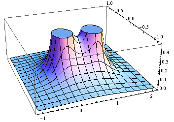
Figure 2: The adiabatic abelian curvature for 3 half fluxes. It is singular when fluxon collides, namely at $u=1$ and $u=0$. It is symmetric under $u\mapsto\bar{u}$. See Eq. (C.5) and Appendix  C for more details on how the figure was drawn.

When $N=2$ and $D=1$ braiding is topological by a special reason that we shall discuss in Sec. 4.6. However, for $N\geq 3$ and $D=1$, the braiding of two fluxons $(a,b)$, keeping all the other fluxons fixed is, in general, path dependent.

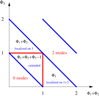
Figure 3: A “phase diagram” for the holonomy of fluxon 3 going around the pair of nearby fluxons $1+2$ i.e. $r_{12}\ll r_{13}$. The diagonal blue lines delineate regions without zero modes, with one zero mode and with 2 zero modes. In the triangle marked by $\Phi_{3}$ the charge is localized on $1+2$ fluxons and Berry’s phase is $2\pi\Phi_{3}$ as one would expect from the Aharonov-Bohm effect. The triangle marked $\Phi_{1}+\Phi_{2}$ describes a zero mode confined on 3 and the phase is $2\pi(\Phi_{1}+\Phi_{2})$. In the triangle marked by $\Phi_{1}+\Phi_{2}+\Phi_{3}-1$ the state is free and the Berry phase is $2\pi(\Phi_{1}+\Phi_{2}+\Phi_{3}-1)$.

4.5 The connection for free states of point-like fluxons

For the sake of simplicity of the notation we shall write $\Phi_{a}=\Phi_{a}^{\prime}<1$ and $D=D_{f}$ in this section.

In Appendix B we show that the metric $\mathbf{g}$ for the free zero modes factorizes into a holomorphic and anti-holomorphic factors. By Eq. (B.10):

$$\mathbf{g}(\zeta;\Phi)=\mathbf{\Psi}^{*}(\zeta;\Phi)\mathbf{G}(\Phi)\mathbf{\Psi}(\zeta;\Phi)$$ (4.6)

where:

• $\mathbf{\Psi}(\zeta,\Phi)$ is an $N\times D$ holomorphic (matrix) function whose matrix elements are given in Eq. (B.5), as

  $$\mathbf{\Psi}_{ak}(\zeta)=\int_{\xi_{0}}^{\zeta_{a}}d\xi\,\psi_{k}(\xi),\quad a\in 1,\dots,N,\quad k\in 0,\dots,D-1$$ (4.7)

  $\mathbf{\Psi}(\zeta,\Phi)$ involves a choice, which we call a gauge choice, and is hidden in the freedom of $\xi_{0}$. Alternatively one could add arbitrary integration constant $c_{k}$ to the r.h.s.

• $\mathbf{G}(\Phi)$ is an $N\times N$ hermitian matrix which is independent of the controls $\zeta\in\mathbb{C}^{N}$. Its explicit form is given in appendix B. It has rank $N-1$ with its kernel generated by the vector $1_{N}=(1,1,...1)^{t}$. Note that this guarantees that the metric $\mathbf{g}$ is not affected by adding arbitrary integration constant to Eq.(4.7).

Substituting the expression (4.6) for the metric into Eq. (3.24) leads to the transport equation

$$\underbrace{{\mathbf{\Psi}}^{*}\,{\mathbf{G}}}_{D\times N}\,{d}\left({\mathbf{\Psi}}{p}\right)=0$$ (4.8)

These are $D$ equations for the evolution of the $D$ coefficients $p\in\mathbb{C}^{D}$. The solutions of these equations are, in general, path dependent. If one could cancel out the left factor $\mathbf{\Psi}^{*}\mathbf{G}$, it would follow that the holonomy is topological. In general however this cannot be done since $\mathbf{\Psi}^{*}\mathbf{G}$ is not an invertible (or even a square) matrix. The holonomy is, in general, not topological.

4.6 Topological holonomy

When the number of free zero modes is maximal

$$D_{f}=N-1$$

the holonomy is topological.

Example 4.2

The simplest example of this kind is $N=2$ and $D_{f}=1$. The Berry phase associated with taking one fluxon around the other is topological and is given by Eq. (4.3) with $k=0$

$$2\pi(\Phi_{T}-1)$$

One way to show that this is the case is by using the ‘gauge’ freedom to choose $\xi_{0}=\zeta_{N}$ in Eq.(4.7) so that $\mathbf{\Psi}_{Nj}=0$ for all $j$. By throwing its last row we can then view $\mathbf{\Psi}$ as a square $D\times D$ matrix which we denote $\mathbf{\Psi}_{\square}$. We may then write for the metric

$$\mathbf{g}_{jk}=\sum_{a,b=1}^{D}\bar{\mathbf{\Psi}}_{aj}G_{ab}\mathbf{\Psi}_{bk}\Longleftrightarrow\mathbf{g}=\mathbf{\Psi}^{*}_{\square}\mathbf{G}_{\square}\mathbf{\Psi}_{\square}$$ (4.9)

where $\mathbf{\Psi}_{\square},\mathbf{G}_{\square},\mathbf{\Psi}^{*}_{\square}$ are all square $D\times$D matrices. Repeating the arguments of the previous subsection Eq. (4.8) now takes the form

$$\mathbf{\Psi}^{*}_{\square}\mathbf{G}_{\square}{d}\left({\mathbf{\Psi}}_{\square}p\right)=0$$ (4.10)

Since $\mathbf{g}$ is positive, all of its ($D\times D$) factors are invertible. The equations of parallel transport therefore reduces into $D$ conservation laws and ${\cal A}$ is a pure gauge :

$$d(\mathbf{\Psi}_{\square}\,p)=0,\quad{\cal A}=\mathbf{g}^{-1}\partial\mathbf{g}=\mathbf{\Psi}^{-1}_{\square}d\mathbf{\Psi}_{\square}$$ (4.11)

It follows that the holonomy of adiabatic transport is determined by the monodromy of the (multivalued function) $\mathbf{\Psi}_{\square}$.

The gauge choice $\xi_{0}=\zeta_{N}$ has the disadvantage of treating $\zeta_{N}$ on different footing than the other $\zeta_{a}$s. Moreover, in braiding operations in which the $N$th fluxon is more than a spectator, any dependence of $\xi_{0}$ on $\zeta_{N}$ can lead to extra complication. For this reason we shall prefer in the next section to fix $\xi_{0}$ to be a constant independent of $\zeta$.

Remark 4.1

One may avoid the ‘gauge’ choice $\xi_{0}=\zeta_{N}$ and rewrite equation (4.11) in a gauge independent way as

$$d(\mathbf{\Psi}\,{p})\in\mathbb{C}\,\mathbf{1}_{N}$$ (4.12)

where $\mathbf{1}_{N}=(1,1,...1)^{t}$ is the generator of $\ker(\mathbf{G})$ and the complex coefficient on the r.h.s depends on the arbitrary integration constant chosen in the definition of $\mathbf{\Psi}$ .

5 Fluxons braiding, non-abelian unitaries and anyons

We have seen that when $D_{f}=N-1$ there is no curvature. Hence, if the unitary holonomy operators are non trivial, and non-abelian, then fluxon braiding can be viewed as (non abelian) topological unitary operations on the manifold of zero modes. We start by computing the monodromy of braiding of distinct fluxons. In the special case that the fluxons carry identical fluxes, they may be viewed as identical anyons. In particular, when the fluxes are identical, it obeys the braiding rules of Burau representation of the braid group.

Figure 4: The convention for ordering the cuts is shown in the case of three point-like fluxons located at $\zeta_{1},\zeta_{2},\zeta_{3}$. With each fluxon one associates a cut $\Sigma$. The cuts define three different regions that extend to infinity. The cuts are ordered so that as one goes counter-clockwise along a big circle (near infinity) the cuts are traversed successively according to their $a$-indexing. We identify $\Sigma_{N+1}$ with $\Sigma_{1}$. The function $\mathbf{\Psi}$ defined in Eq. (5.1), takes different limiting values at $\infty_{a}$.

5.1 The monodromy of braiding fluxes

We start by computing the monodromy of $\mathbf{\Psi}$. In subsection 5.3 we shall relate it to the holonomy of the adiabatic evolution.

The components of the matrix $\mathbf{\Psi}$ are by Eq. (4.7),

$$\mathbf{\Psi}_{aj}(\zeta)=\int_{\xi_{0}}^{\zeta_{a}}d\xi\ \xi^{j}\prod_{b=1}^{N}(\xi-\zeta_{b})^{-\Phi_{b}}$$ (5.1)

Since $j$ is an integer the factor $\xi^{j}$ in the integrand has no interesting effect on the monodromy and we can ignore the index $j$ (and henceforth drop it) without risk.

Choosing integration paths from $\xi_{0}$ to $\zeta_{1},\dots,\zeta_{N}$ which do not cross any of the cuts shown in Fig. 4 leads to a standard definition of $\Psi=(\Psi_{1},\dots,\Psi_{N})^{t}$. Upon cyclically moving the fluxon positions $\zeta_{a}$ these paths are deformed as seen in Figs. 5,6 into paths which typically do cross the cuts. This leads to another branch $\Psi^{\prime}=(\Psi_{1}^{\prime},\dots,\Psi_{N}^{\prime})^{t}$ of the multivalued function. The monodromy is an $N\times N$ matrix $\mathbf{M}$:

$$\Psi^{\prime}=\mathbf{M}\Psi,\quad\Psi=(\Psi_{1},\dots,\Psi_{N})^{t}$$ (5.2)

It is useful to collect properties of $\mathbf{M}$ before one actually computes it, as they provide tests on the computations.

• Since the fluxons may be moved backwards, the monodromies $\mathbf{M}$ must be invertible and generate a group.

• Since $\mathbf{g}$ (of Eq. (4.6)) must not be affected by the monodromy, $\mathbf{M}$ and $\mathbf{G}$ must satisfy a consistency condition

  $$\mathbf{G}=\mathbf{M}^{*}\mathbf{G}\mathbf{M}$$ (5.3)

  (This may be viewed as a unitarity condition).

• Adding an integration constant (or equivalently changing $\xi_{0}$) in Eq. (5.1) corresponds to $\Psi\mapsto\Psi+c\mathbf{1}_{N}$ and $\Psi^{\prime}\mapsto\Psi^{\prime}+c\mathbf{1}_{N}$. Consistency with Eq.(5.2) thus requires

  $$\mathbf{M}\,\mathbf{1}_{N}=\mathbf{1}_{N}$$

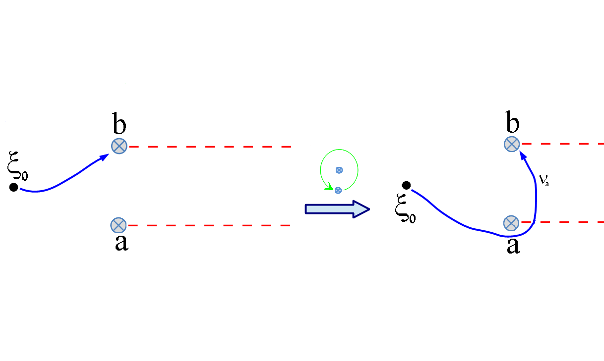
Figure 5: The figure shows fluxon $a$ with its (red dashed) branch cut $\Sigma_{a}$ going counter clock-wise around fluxon $b=a+1$ with its (red dashed) branch cut $\Sigma_{b}$. As $a$ encircles $b$ the integration path (blue) from $\xi_{0}$ to $\zeta_{b}$ loops around the branch point of the cut $\Sigma_{a}$. The integration from $a$ to $b$ in the old and new paths are related by a factor $\nu_{a}$.

A proper definition of the monodromy of $\Psi$ requires choosing some definite convention for placements of the cuts, see Fig. 4. We shall take the cut $\Sigma_{a}$ to run from $\zeta_{a}$ to $\infty$, and we order them in such a way that as one goes counter-clockwise along a big circle (near infinity) the cuts $\Sigma_{a}$ are traversed successively according to their $a$-indexing.

Let us now compute the monodromy as the flux ${a}$ encircles an adjacent flux ${b}=a+1$ counter-clockwise. The integration path associated with $\Psi_{b}$ loops around the branch point $a$ as shown in Fig. 5. The deformed path gives

$$(\Psi^{\prime})_{b} =\int_{\xi_{0}}^{\zeta_{a}}\psi(z)dz+\nu_{a}\int_{\zeta_{a}}^{\zeta_{b}}\psi(z)dz$$

$$=\Psi_{a}+\nu_{a}(\Psi_{b}-\Psi_{a})$$ (5.4)

By similar considerations as $a$ loops around $b$, the integration path associated with $\Psi_{a}$ “stitches” $b$ as shown in Fig. 6. It follows that

$$(\Psi^{\prime})_{a} =\int_{\xi_{0}}^{\zeta_{a}}\psi(z)dz+\nu_{a}\int_{\zeta_{a}}^{\zeta_{b}}\psi(z)dz+\nu_{b}\nu_{a}\int_{\zeta_{b}}^{\zeta_{a}}\psi(z)dz$$

$$=\Psi_{a}+\nu_{a}(\Psi_{b}-\Psi_{a})+\nu_{a}\nu_{b}(\Psi_{a}-\Psi_{b})$$

$$=\big{(}1-\nu_{a}+\nu_{a}\nu_{b}\big{)}\Psi_{a}+\nu_{a}(1-\nu_{b})\Psi_{b}$$ (5.5)

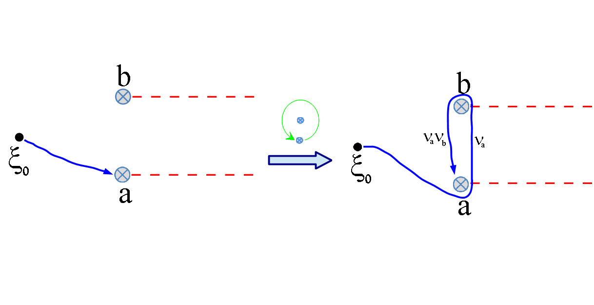
Figure 6: The deformation of the path of integration from the fiducial point $\xi_{0}$ to the fluxon at $\zeta_{a}$. As the $a$-th fluxons encircle b counter-clockwise it “stitches” $b$. The old and new values of $\Psi_{a}$ differ by integrations from $a$ to $b$ along two sides of the two cuts.

All other components of $\Psi$ remain unaffected. The $2\times 2$ nontrivial block of the monodromy matrix is therefore

$$\mathbf{M}(\nu_{a},\nu_{b})={\left(\begin{array}[]{cc}1-\nu_{a}+\nu_{a}\nu_{b}&\nu_{a}(1-\nu_{b})\\ 1-\nu_{a}&\nu_{a}\end{array}\right)},\quad\det\mathbf{M}=\nu_{a}\nu_{b}$$ (5.6)

The monodromy matrix is not symmetric in $a,b$ due to our convention for ordering the cuts counter clockwise. $\mathbf{M}(\nu_{a},\nu_{b})$ is related to $\mathbf{M}(\nu_{b},\nu_{a})$ by

$$\mathbf{M}(\nu_{b},\nu_{a})=\sigma_{x}\mathbf{M}^{-1}(\bar{\nu}_{a},\bar{\nu}_{b})\sigma_{x}$$

By Eq.(5.3) the spectrum of $M$ should lie on the unit circle.

Indeed:

$$Eigenvalues(\mathbf{M})=\{1,\nu_{a}\nu_{b}\}$$ (5.7)

5.2 Braiding identical fluxes

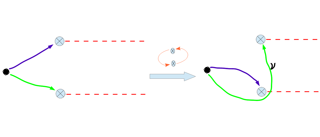
Figure 7: Exchanging identical fluxes

In the special case where all fluxons are identical (having the same $\Phi_{a}$) it makes sense to consider also a permutation of two adjacent fluxons. This leads to the Burau representation of the braid group [7].

Indeed, inspecting Fig. 7 we see

$$(\Psi^{\prime})_{a} =\ \Psi_{a}+\nu(\Psi_{b}-\Psi_{a})$$ (5.8)

$$(\Psi^{\prime})_{b} =\Psi_{a}$$

The monodromy matrix has the single nontrivial $2\times 2$ block

$$\mathbf{M}(\nu)={\left(\begin{array}[]{cc}1-\nu&\nu\\ 1&0\end{array}\right)},\quad\det\,\mathbf{M}=-\nu$$ (5.9)

with eigenvalues $\{1,-\nu\}$. Note that when $\nu\rightarrow 1$ this reduces to the standard representation of the symmetric group. This may be understood as due to the fact that in this limit the free zero-modes turn into confined modes which move with the fluxons. The case $\nu=-1$ (i.e. $\Phi_{a}={1\over 2}$) does not occur since it is inconsistent with the assumption $D_{f}=N-1$, see Eq. (1.5).

5.3 The non-abelian holonomy

The (non-abelian) holonomy $\mathbf{U}(\gamma,\zeta)$ for a closed path $\gamma$ and base point $\zeta$, acts unitarily on the $D_{f}=N-1$ dimensional space of (free) zero modes at $\zeta$:

$$\mathbf{U}:\sum p_{j}|\psi_{j}\rangle\mapsto\sum p_{j}^{\prime}|\psi_{j}.\rangle$$

One may write $\mathbf{U}|\psi_{j}\rangle=\sum u_{ij}|\psi_{i}\rangle$ or equivalently $p_{i}^{\prime}=\sum u_{ij}p_{j}$. Since the basis $\{|\psi_{j}\rangle\}$ is not orthonormal, the matrix $\mathbf{u}$ is not unitary. Instead it satisfies $\mathbf{u}^{*}\mathbf{g}\mathbf{u}=\mathbf{g}$. This is consistent with unitarity of the holonomy operator

$$\mathbf{U}=\sum|\psi_{j}\rangle\left(ug^{-1}\right)_{ji}\langle\psi_{i}|$$

The previous sections make it clear that on the $D_{f}=N-1$ dimensional space of free zero modes, the $(N-1)\times(N-1)$ matrix $u$ is closely related to the $N\times N$ monodromy matrix $M$. The exact relation is however complicated by the ’gauge’ freedom of fixing $\xi_{0}$. We would like in this section to state this relation more precisely.

For simplicity, consider first only braidings which do not involve the $N$-th fluxon. Using the ’gauge’ choice $\xi_{0}=\zeta_{N}$ one writes the conservation law, Eq. (4.11), taking ${p}$ around a closed path (based at $\zeta$):

$$\mathbf{\Psi}_{\square}\,{p}=\mathbf{\Psi^{\prime}}_{\square}\,{p^{\prime}}=\mathbf{M}_{\square}\mathbf{\Psi}_{\square}\,{p^{\prime}}$$ (5.10)

($\mathbf{M}_{\square}$ is the $D\times D$ matrix obtained from $\mathbf{M}$ by deleting its last row and column.) The last identity used the definition of $\mathbf{M},$ Eq. (5.2). Hence

$$p_{i}^{\prime}=\sum_{j}u_{ij}p_{j},\quad\mathbf{u}=(\mathbf{\Psi}_{\square})^{-1}\mathbf{M}^{-1}_{\square}\mathbf{\Psi}_{\square}$$ (5.11)

The derivation given above was special to the case where $\zeta_{N}$ was a spectator. Below we give an analysis of the general case.

The monodromy matrices $M$ acting on $\mathbb{C}^{N}$ preserve the vector $\mathbf{1}_{N}\in\mathbb{C}^{N}$ i.e. satisfy $M\mathbf{1}_{N}=\mathbf{1}_{N}$. It follows that $M$ defines a linear transformation $\tilde{M}$ on the quotient space $V_{0}=\mathbb{C}^{N}/\mathbb{C}\,\mathbf{1}_{N}$. We shall show that the holonomy $\mathbf{U}(\gamma,\zeta)$ for a closed path $\gamma$ and base point $\zeta$ is obtained from $\tilde{M}$ by a similarity transformation.

The hermitian matrix $G$ satisfies $G\mathbf{1}_{N}=0$. Therefore the hermitian form it defines on $\mathbb{C}^{N}$, projects to a hermitian form $\tilde{G}$ on $V_{0}=\mathbb{C}^{N}/\mathbb{C}\,\mathbf{1}_{N}$. Moreover since $G$ has $D$ positive eigenvalues the form $\tilde{G}$ must give a (non degenerate) inner product on $V_{0}$. Eq. (5.3) shows that $\tilde{M}$ are unitary relative to this inner product on $V_{0}$.

By Eq.(4.12) and the definition of the monodromy $M$ one has

$$M\mathbf{\Psi}p^{\prime}=\mathbf{\Psi}p\;\mod\,\mathbf{1}_{N}$$

Recall that $\mathbf{\Psi}$ is an $N\times(N-1)$ matrix i.e. a map $\mathbb{C}^{N-1}\rightarrow\mathbb{C}^{N}$. Denoting by $\tilde{\mathbf{\Psi}}$ the corresponding map into $V_{0}=\mathbb{C}^{N}/\mathbb{C}\,\mathbf{1}_{N}$ we conclude

$$\tilde{M}\tilde{\mathbf{\Psi}}p^{\prime}=\tilde{\mathbf{\Psi}}p$$

As $\tilde{\mathbf{\Psi}}$ is clearly invertible (as follows e.g. from $\tilde{\mathbf{\Psi}}^{*}\tilde{G}\tilde{\mathbf{\Psi}}=g$), we see that

$$u=\tilde{\mathbf{\Psi}}^{-1}\tilde{M}^{-1}\tilde{\mathbf{\Psi}}$$

In particular the eigenvalues of the holonomy $\mathbf{U}$ of fluxon braiding are related to the eigenvalues of the monodromy $M$ by

$$Eigenvalues(\mathbf{M})=Eigenvalues(\tilde{\mathbf{M}})\cup\{1\}=Eigenvalues(\mathbf{U}^{-1})\cup\{1\}$$ (5.12)

It follows from the results of the previous sections that when the fluxon $a$ goes around the fluxon $b$, the holonomy matrix eigenvalues are

$$Eigenvalues(\mathbf{U})=\{1,\bar{\nu}_{a}\bar{\nu}_{b}\}$$ (5.13)

Remark 5.1

By considering the $N\times N$ matrix $\Lambda(\zeta)={\left(\begin{array}[]{cc}\mathbf{\Psi}&\mathbf{1}_{N}\end{array}\right)}$ obtained by adding $\mathbf{1}_{N}$ as an extra column to $\mathbf{\Psi}(\zeta)$ and defining

$$|a\rangle=\sum_{j=0}^{D-1}{\Lambda}^{-1}_{ja}|\psi_{j}\rangle,\,a=1,...N$$

we can obtain the simple relation $\mathbf{U}|a\rangle=(\mathbf{M}^{-1})_{ba}|b\rangle$ as well as $\langle a|b\rangle=G_{ab}$. The set $\{|a\rangle\}$ is however an over-spanning set rather than a basis as it satisfies $\sum|a\rangle=0$.

Acknowledgement: The research is supported by ISF. We thank M. Fraas, Y. Aharonov, N. Lindner, A. Ori, N. Cohen and P. Seba for discussions.

Appendix A Construction of the confined modes

For the sake of simplicity we take that $\Phi_{a}$ is not an integer and assume that $\Phi_{T}^{\prime}\equiv\sum\Phi_{a}^{\prime}>0$. (In particular this is the case if $\Phi_{a}>0$ for all $a$.) This guarantees that the $D_{f}=\lceil\Phi_{T}^{\prime}\rceil-1$ free modes we constructed are indeed square integrable at infinity. Since the total number of zero modes is determined by $\sum\Phi_{a}=\sum n_{a}+\sum\Phi_{a}^{\prime}$ there must be $\sum n_{a}$ confined modes.

For a single super-critical fluxon $\Phi_{a}>1$ we saw in section 2.1.1 that as $R\rightarrow 0$ we obtain $n_{a}=\lfloor\Phi_{a}\rfloor$ modes $\psi_{a}^{j}$ all localized in a small $O(R)$ neighbourhood of it. Consider the multi-fluxon case. By our superposition principle one may construct $\psi$ as a product of (not necessarily fundamental) solutions $\psi_{b}$ corresponding to all fluxons. In particular $n_{a}$ solutions concentrated near a specific fluxon $a$ may be constructed as follows. Take $\psi_{a}=\psi_{a}^{j}$ and for any $b\neq a$ choose $\psi_{b}=(z-\zeta_{b})^{n_{b}}(\psi_{b})_{0}$. The resulting zero-mode $\psi=\psi_{a}^{j}\prod_{b\neq a}\psi_{b}$ is then concentrated in a region of radius $O(R)$ near $z=\zeta_{a}$. Indeed for any $b\neq a$ it remains square integrable at $z\rightarrow\zeta_{b}$ even in the limit $R_{b}=0$ while near $z=\zeta_{a}$ it behaves just like the single fluxon solutions $\psi_{a}^{i}$. In fact assuming (as always) $R_{a}\ll|\zeta_{a}-\zeta_{b}|$ one may approximate it a

$$\psi(z)=\psi_{a}^{j}(z)\prod_{b\neq a}\psi_{b}(z)\simeq\psi_{a}^{j}(z)\prod_{b\neq a}\psi_{b}(\zeta_{a}).$$

We conclude that there are $n_{a}$ localized modes near each super-critical fluxon as well as $\lfloor\sum\Phi_{a}^{\prime}\rfloor$ free states. Modes localized on different fluxons are clearly mutually orthogonal. Some extra thought also shows that when properly normalized the overlap of free state with a confined state localized at $\mathbf{r}_{a}$ scales as $R_{a}^{1-\Phi_{a}^{\prime}}$ and hence vanishes in the pointlike limit.

If $\Phi_{T}^{\prime}<0<\Phi_{T}$ as can happen when some of the fluxons are negative then the above construction might fail. In such case one finds there are no free states and only part of the localized states survive (others being turned into resonances). As an example consider $N=3$ with $\Phi=(3/2,3/2,-3/2)$. In this case $\Phi_{T}=3/2$ implies there is only $D=1$ zero mode, which tries to be localized on two supercritical fluxons. What will actually happen is that one superposition of confined states will remain a true state while the other will turn into a resonance.

Appendix B Factorization of the metric

In this section we show that the metric $\mathbf{g}$ for the free modes of point-like fluxons factorizes into a product of a holomorphic and anti-holomorphic factors. Since we are interested only in the free states, we will, for notational simplicity, assume all fluxons are subcritical. If this is not the case one should replace $\Phi_{a}$ by its fractional part.

Let $\mathbf{\Psi}_{j}$ denote the primitive integral of $\psi_{j}$:

$$\Psi_{j}(z;\zeta,\xi_{0})=\int_{\xi_{0}}^{z}d\xi\,\psi_{j}(\xi),\quad\psi_{j}(\xi)=\xi^{j}\prod_{a}(\xi-\zeta_{a})^{-\Phi_{a}},\quad j=0,\dots,D-1$$ (B.1)

We shall refer to the choice of $\xi_{0}$ as a choice of a gauge.

For $N=2,3$ Mathematica can evaluate $\Psi_{j}$ of Eq. (B.1) in terms of known special functions. In general, when $N\geq 4$ the integral form is the best we can do.

Since $dx\wedge dy=\frac{i}{2}dz\wedge d\bar{z}$ one of the two integrations in Eq. (3.21) for the metric is for free

$$\mathbf{g}_{jk}=\frac{i}{2}\int d{\Psi}_{k}\wedge d\bar{\Psi}_{j}=\frac{i}{2}\sum_{a}\int_{\Sigma_{a}}{\Psi}_{k}{\bar{\psi}}_{j}d\bar{z}$$ (B.2)

And we have used the generalized Stokes theorem. The remaining contour integrals encircle the cuts $\Sigma_{a}$ running from $\zeta_{a}$ to $\infty$ (See Fig. 4).

The value of $\psi_{j}$ above and below the cut are related by

$${(\psi_{j})}_{-}=\nu_{a}{(\psi_{j})}_{+}\quad\nu_{a}=e^{-2\pi i\Phi_{a}}$$ (B.3)

To see how $\Psi_{k}$ behaves across the cut $\Sigma_{a}$ write

$$\Psi_{k}(z;\zeta,\xi_{0})=\mathbf{\Psi}_{ak}(\zeta)+\Psi_{k}(z;\zeta,\zeta_{a}),$$ (B.4)

where

$$\mathbf{\Psi}_{ak}(\zeta)={\Psi}_{k}(\zeta_{a};\zeta,\xi_{0})=\int_{\xi_{0}}^{\zeta_{a}}d\xi\,{\xi^{k}}\psi_{0}(\xi),$$ (B.5)

The first term is a finite constant (independent of $z$). The second term inherits the $\nu_{a}$ discontinuity of $\psi_{j}$. It follows that $\Psi_{k}(z;\zeta,\zeta_{a})\bar{\psi}_{j}(z)$ is continuous across the cut $\Sigma_{a}$ and does not contribute to the integral in Eq. (B.2). The metric reduces to

$$\mathbf{g}_{jk} =\frac{i}{2}\sum_{a}\mathbf{\Psi}_{ak}(\zeta)\int_{\Sigma_{a}}{\bar{\psi}}_{j}d\bar{z}$$ (B.6)

$$=\frac{i}{2}\sum_{a}\mathbf{\Psi}_{ak}(\zeta)(1-\bar{\nu}_{a})\big{(}\bar{\Psi}_{j}(\infty_{a};\zeta,\xi_{0})-\bar{\mathbf{\Psi}}_{aj}(\zeta)\big{)}$$

We denote by ${\Psi}_{j}(\infty_{a};\zeta,\xi_{0})$ the value attained by ${\Psi}_{j}(z;\zeta;\xi_{0})$ as $z$ tends to infinity in the region between the cuts $\Sigma_{a}$ and $\Sigma_{a+1}$. (See Fig. 4.) The limit is well defined at infinity provided $j\leq D-1$, which is what we need for the metric.

Rewrite Eq. (B.6) as a matrix equation

$$\mathbf{g}=\left(\mathbf{\Psi}_{\infty}-\mathbf{\Psi}\right)^{*}\mathbf{G}_{1}\mathbf{\Psi},\quad(\mathbf{G}_{1})_{ab}=\frac{i}{2}\delta_{ab}(1-\bar{\nu}_{a})$$ (B.7)

$\mathbf{G}_{1}(\Phi)$ is independent of $\zeta$.

The $N$-tuples $\mathbf{\Psi}_{\infty}=\big{(}{\Psi}_{j}(\infty_{1}),\dots,{\Psi}_{j}(\infty_{N})\big{)}$ and $\mathbf{\Psi}=({\Psi}_{1j},\dots,{\Psi}_{Nj})$ are linearly dependent

$${\Psi}_{j}(\infty_{a-1})-{\Psi}_{aj}=\nu_{a}({\Psi}_{j}(\infty_{a})-{\Psi}_{aj}),\quad a\in 1,\dots,N$$ (B.8)

where ${\Psi}_{j}(\infty_{N})={\Psi}_{j}(\infty_{0})$. This comes from integrating ${\psi}_{-}=\nu_{a}{\psi}_{+}$ along $\Sigma_{a}$. Eq. (B.8) too may be written as a matrix equation

$$\mathbf{G}_{2}\mathbf{\Psi}_{\infty}=\mathbf{\bar{G}}_{1}\mathbf{\Psi},\quad(\mathbf{G}_{2})_{ab}=\frac{i}{2}(\delta_{ab}\nu_{a}-\delta_{a,b+1})$$ (B.9)

It follows from Eq. (B.7) and Eq. (B.9) that the $D\times D$ matrix $\mathbf{g}$ can be factored as

$$\mathbf{g}(\zeta;\Phi)=\mathbf{\Psi}^{*}(\zeta;\Phi)\mathbf{G}(\Phi)\mathbf{\Psi}(\zeta;\Phi),\quad\ \mathbf{G}=\left(\mathbf{\bar{G}}_{1}^{*}\left(\mathbf{G}_{2}^{-1}\right)^{*}-\mathbbm{1}\right)\mathbf{G}_{1}$$ (B.10)

where:

• $\mathbf{\Psi}(\zeta,\Phi)$ is an $N\times D$ holomorphic (matrix) function whose matrix elements are given in Eq. (B.5).

• $\mathbf{G}(\Phi)$ is an $N\times N$ matrix which is independent of the controls $\zeta\in\mathbb{C}^{N}$.

• Since $\mathbf{g}$ is a $D\times D$ positive matrix, $\mathbf{G}$ must be an hermitian matrix. It must have at least $D$ positive eigenvalues and the image of $\mathbf{\Psi}$ must lie in the “positive cone” of $\mathbf{G}$. In fact one may show that $\mathbf{G}$ has exactly $D$ positive eigenvalues.

• The definition of $\mathbf{\Psi}_{j}$ as a primitive integral in Eq. (B.1) allows addition of an arbitrary integration constant (possibly $j$-dependent) corresponding to a free choice of $\xi_{0}$. Change of this choice will change the columns of $\mathbf{\Psi}$ by constant columns:

  $$\delta\mathbf{\Psi}=\left(\begin{array}[]{ccc}\delta c_{1}&\dots&\delta c_{D}\\ \dots&\dots&\dots\\ \delta c_{1}&\dots&\delta c_{D}\end{array}\right)$$ (B.11)

  Since changing $\xi_{0}$ must not affect the metric, it follows that the kernel of $\mathbf{G}$ contains the vector $(1,\dots,1)^{t}$. It is in fact spanned by it.

• One convenient ‘gauge’ choice is $\xi_{0}=\zeta_{N}$ which makes the last row of $\mathbf{\Psi}_{aj}(\zeta)$ vanish. As a result Eq. (B.10) takes the form $g=\check{\mathbf{\Psi}}^{*}\check{\mathbf{G}}\check{\mathbf{\Psi}}$ where $\check{\mathbf{\Psi}}$ is $(N-1)\times D$ and $\check{\mathbf{G}}$ is $(N-1)\times(N-1)$.

• An explicit expression for $\mathbf{G}$ is

  $$\mathbf{G}_{ab}=\frac{\sin\left(\pi\Phi_{a}\right)}{\sin\left(\pi\Phi_{T}\right)}\times\begin{cases}-\sin\left(\pi(\Phi_{T}-\Phi_{a})\right)&a=b\\ \sin\left(\pi\Phi_{b}\right)\exp\left[i\pi\left(\Phi_{T}-\sum_{c=a}^{b-1}(\Phi_{c}+\Phi_{c+1})\right)\right]&a<b\end{cases}$$ (B.12)

  The values for $N\geq a>b\geq 1$ may be deduced from hermiticity condition $G_{ab}=G_{ba}^{*}$. Alternatively the same value may be found from the relation $G_{ab}=G_{a,b+N}$.

• When all the fluxes are identical $\mathbf{G}$ is a Töplitz matrix, i.e. constant along the diagonals,

  $$\mathbf{G}_{ab}=G_{a-b},\quad a,b\in 1,\dots,N$$ (B.13)

  Explicitly, if each fluxon carries $\Phi_{a}=\Phi$, then for ,$0<k\leq N$,

  $$G_{0}=-{\sin\left({\pi\Phi}\right)\sin\left({\pi\Phi(N-1)}\right)\over\sin(\pi N\Phi)},\quad G_{k}=e^{i\pi\Phi(N-2k)}\frac{\sin^{2}\left({\pi\Phi}\right)}{\sin(\pi N\Phi)}$$ (B.14)

• Away from the threshold for appearance of a new zero-mode, $\Phi_{T}\in\mathbb{Z}$, the elements of $\mathbf{G}$ are well defined and free of singularities. (As are the elements of $\Psi,\mathbf{g}$.)

Appendix C Three subcritical fluxes

Example C.1

For three half fluxes: $\Phi_{1}=\Phi_{2}=\Phi_{3}=1/2$ at $\zeta_{1}=0,\ \zeta_{2}=1,\ \zeta_{3}=u$

$$\Psi(z;u;0) =\int_{0}^{z}\frac{dx}{\sqrt{x(x-1)(x-u)}}$$

$$=-2iK(1-u)+2iF\left(\left.i\sinh^{-1}(1/\sqrt{z-1})\right|1-u\right)$$ (C.1)

$K(m)$ and $F(\phi|m)$ are elliptic functions and

$$\sinh^{-1}(1/\sqrt{x-1})=\log(\sqrt{x}+1)-\frac{i}{2}\log(x-1)$$

For three fluxons one can find explicit expressions for the metric $\mathbf{g}$ and the curvature. Exploiting translation rotation and dilatation symmetries allow us to fix the location of two fluxons at will. We shall therefore assume the three fluxon are located at $\zeta_{1}=0,\ \zeta_{2}=1,\ \zeta_{3}=u$.

C.1 The abelian case: $1<\Phi_{T}<2$

Choosing $\xi_{0}=\zeta_{1}=0$ leads in the case $D=1$ to the following

$$\mathbf{\Psi}=\left(\begin{array}[]{c}0\\ u^{-\Phi_{3}}{\Gamma\left(1-\Phi_{1}\right)\Gamma\left(1-\Phi_{2}\right)\over\Gamma\left(2-\Phi_{1}-\Phi_{2}\right)}{\,}_{2}\tilde{F}_{1}\left(1-\Phi_{1},\Phi_{3};2-\Phi_{1}-\Phi_{2};{1\over u}\right)\\ u^{1-\Phi_{1}-\Phi_{3}}{\Gamma\left(1-\Phi_{1}\right)\Gamma\left(1-\Phi_{3}\right)\over\Gamma\left(2-\Phi_{1}-\Phi_{3}\right)}{\,}_{2}\tilde{F}_{1}\left(1-\Phi_{1},\Phi_{2};2-\Phi_{1}-\Phi_{3};u\right)\\ \end{array}\right)$$ (C.2)

Here ${\,}_{2}\tilde{F}_{1}$ is a hypergeometric function. For three identical fluxes $\Phi_{a}=\Phi$ this reduces into

$$\mathbf{\Psi}={\Gamma\left(1-\Phi\right)^{2}\over\Gamma\left(2-{2\Phi}\right)}\left(\begin{array}[]{c}0\\ u^{-\Phi}F\left(\frac{1}{u}\right)\\ u^{1-2\Phi}\,F(u)\\ \end{array}\right),\quad F\left(u\right)={\,}_{2}\tilde{F}_{1}\left(1-\Phi,\Phi;2-{2\Phi};{u}\right)$$ (C.3)

In particular in the special case $\Phi=1/2$ it becomes

$$\mathbf{\Psi}=\left(\begin{array}[]{cc}0\\ {2\over\sqrt{u}}K\left({1\over u}\right)\\ 2K(u)\\ \end{array}\right)$$ (C.4)

with $K(m)$ the complete elliptic integral of the first kind. Using Eq. (B.14) for $\mathbf{G}$, one then finds a simple formula for the metric

$$\mathbf{g}(u)=8Re\left(K(u)K(1-u)^{*}\right)$$ (C.5)

The associated curvature is plotted in Fig. (2).

Since $\mathbf{\Psi}$ is defined only up to addition of an arbitrary ($u$-dependent) multiple of $\mathbf{1}_{N}$, one may write down various alternative expressions to Eq. (C.2). Using the following

$$\mathbf{\Psi}= {\pi\Gamma(\Phi_{1}+\Phi_{3}-1)\over\Gamma(\Phi_{1})\Gamma(\Phi_{3})}\left(\begin{array}[]{c}{e^{i\Phi_{1}\pi}\over\sin(\Phi_{1}\pi)}\\ 0\\ -{e^{-i\Phi_{3}\pi}\over\sin(\Phi_{3}\pi)}\\ \end{array}\right)u^{1-\Phi_{1}-\Phi_{3}}\,_{2}\tilde{F}_{1}\left(1-\Phi_{1},\Phi_{2},2-\Phi_{1}-\Phi_{3};u\right)$$ (C.9)

$$+ {\Gamma(1-\Phi_{2})\Gamma(1-\Phi_{1}-\Phi_{3})\over\Gamma(2-\Phi)}e^{-i\pi\Phi_{3}}\left(\begin{array}[]{c}0\\ 1\\ 0\\ \end{array}\right)\,_{2}\tilde{F}_{1}\left(\Phi_{3},\Phi-1,\Phi_{1}+\Phi_{3};u\right)$$ (C.13)

with $\mathbf{G}$ the $3\times 3$ matrix given in Eq. (B.12), leads to expressing the $1\times 1$ metric $\mathbf{g}$ as a combination of two squares

$$\mathbf{g}= \pi{\Gamma(1-\Phi_{2})\over\Gamma(\Phi_{2})}{\Gamma(1-\Phi_{1}-\Phi_{3})\over\Gamma(\Phi_{1}+\Phi_{3})}{\Gamma(\Phi-1)\over\Gamma(2-\Phi)}\left|\,{}_{2}\tilde{F}_{1}\left(\Phi_{3},\Phi-1,\Phi_{1}+\Phi_{3},u\right)\right|^{2}$$

$$+\pi{\Gamma(1-\Phi_{1})\over\Gamma(\Phi_{1})}{\Gamma(1-\Phi_{3})\over\Gamma(\Phi_{3})}{\Gamma(\Phi_{1}+\Phi_{3}-1)\over\Gamma(2-\Phi_{1}-\Phi_{3})}\left|u^{1-\Phi_{1}-\Phi_{3}}\,_{2}\tilde{F}_{1}\left(1-\Phi_{1},\Phi_{2},2-\Phi_{1}-\Phi_{3},u\right)\right|^{2}$$

For $1<\Phi_{T}<3$ this is always positive.

C.2 The non-abelian case: $2<\Phi_{T}<3$

One can also get explicit formulas for the non-abelian case. $\mathbf{\Psi}$ is $3\times 2$:

$$\mathbf{\Psi}=u^{-\Phi_{3}}\left(\begin{array}[]{cc}0&0\\ {\Gamma(1-\Phi_{1})\Gamma(1-\Phi_{2})\over\Gamma(2-\Phi_{1}-\Phi_{2})}\,_{2}\tilde{F}_{1}\left(1-\Phi_{1},\Phi_{3},2-\Phi_{1}-\Phi_{2},{1\over u}\right)&{\Gamma(2-\Phi_{1})\Gamma(1-\Phi_{2})\over\Gamma(3-\Phi_{1}-\Phi_{2})}\,_{2}\tilde{F}_{1}\left(2-\Phi_{1},\Phi_{3},3-\Phi_{1}-\Phi_{2},{1\over u}\right)\\ u^{1-\Phi_{1}}{\Gamma(1-\Phi_{1})\Gamma(1-\Phi_{3})\over\Gamma(2-\Phi_{1}-\Phi_{3})}\,_{2}\tilde{F}_{1}\left(1-\Phi_{1},\Phi_{2},2-\Phi_{1}-\Phi_{3},u\right)&u^{2-\Phi_{1}}{\Gamma(2-\Phi_{1})\Gamma(1-\Phi_{3})\over\Gamma(3-\Phi_{1}-\Phi_{3})}\,_{2}\tilde{F}_{1}\left(2-\Phi_{1},\Phi_{2},3-\Phi_{1}-\Phi_{3},u\right)\\ \end{array}\right)$$ (C.14)

$$\mathbf{\Psi}=u^{-\Phi_{3}}\left(\begin{array}[]{cc}0&0\\ \frac{\Gamma(1-\Phi_{1})\Gamma(1-\Phi_{2})}{\Gamma(2-\Phi_{1}-\Phi_{2})}\,A&\frac{\Gamma(2-\Phi_{1})\Gamma(1-\Phi_{2})}{\Gamma(3-\Phi_{1}-\Phi_{2})}\,B\\ u^{1-\Phi_{1}}\frac{\Gamma(1-\Phi_{1})\Gamma(1-\Phi_{3})}{\Gamma(2-\Phi_{1}-\Phi_{3})}\,C&u^{2-\Phi_{1}}\frac{\Gamma(2-\Phi_{1})\Gamma(1-\Phi_{3})}{\Gamma(3-\Phi_{1}-\Phi_{3})}\,D\\ \end{array}\right)$$ (C.15)

where

$$A={\,}_{2}\tilde{F}_{1}\left(1-\Phi_{1},\Phi_{3},2-\Phi_{1}-\Phi_{2},\frac{1}{u}\right) \quad B={\,}_{2}\tilde{F}_{1}\left(2-\Phi_{1},\Phi_{3},3-\Phi_{1}-\Phi_{2},\frac{1}{u}\right)$$

$$C={\,}_{2}\tilde{F}_{1}\left(1-\Phi_{1},\Phi_{2},2-\Phi_{1}-\Phi_{3},u\right) \quad D={\,}_{2}\tilde{F}_{1}\left(2-\Phi_{1},\Phi_{2},3-\Phi_{1}-\Phi_{3},u\right)$$

When all three fluxes are identical $\Phi_{a}=\Phi$ this becomes

$$\mathbf{\Psi}={\Gamma\left(1-\Phi\right)^{2}\over 2\Gamma\left(2-{2\Phi}\right)}\left(\begin{array}[]{cc}0&0\\ 2u^{-\Phi}F\left(\frac{1}{u}\right)&\,u^{-\Phi}G\left(\frac{1}{u}\right)\\ 2u^{1-2\Phi}\,F(u)&u^{2-2\Phi}\,G(u)\\ \end{array}\right)$$ (C.16)

where

$$F\left(u\right)={\,}_{2}\tilde{F}_{1}\left(1-\Phi,\Phi;2-2\Phi;{u}\right),\quad G(u)={\,}_{2}\tilde{F}_{1}\left(2-\Phi,\Phi;3-2\Phi;u\right)$$

$\mathbf{G}$ is again $3\times 3$ given by Eq. (B.12) and $\mathbf{g}$ is $2\times 2$.

Appendix D An abstract construction of the adiabatic connection.

In this appendix we give another (more abstract) construction of the connection described in Sec. 4.5 and Sec. 4.6 corresponding to the free zero modes around point-like fluxons. In particular it shows that in general one may embed our $D_{f}$-dimensional bundle into a flat $N-1$ bundle.

Let $V_{0}$ be the fixed $(N-1)$-dimensional complex vector space $\mathbb{C}^{N}/\mathbb{C}\,\mathbf{1}_{N}$ where $\mathbf{1}_{N}=(1,1,...1)^{t}$. Since $ker(G)=\mathbb{C}\,\mathbf{1}_{N}$, the $N\times N$ hermitian matrix $G$ defines a pseudo (hermitian) metric on $V_{0}$. Let ${\cal M}=\{(\zeta_{1},\zeta_{2},...\zeta_{N})\in\mathbb{C}^{N}|\;\forall a\neq b\;\;\zeta_{a}\neq\zeta_{b}\}$ be the space of possible positions of $N$ fluxons. Consider the trivial bundle $E_{0}={\cal M}\times V_{0}$. For each $j$ the vector function $\Psi_{j}(\zeta)=(\Psi_{1j},\Psi_{2j},...\Psi_{Nj})$ defines a (multivalued) section of $E_{0}$. We shall denote this section by $\Psi_{j}$ as well although it is actually an equivalence class under quotienting by $\mathbf{1}_{N}=(1,1...1)^{t}$.

At each point $\zeta\in{\cal M}$ the vectors $\Psi_{0}(\zeta),...\Psi_{D-1}(\zeta)$ generate a $D$-dimensional subspace $V_{\zeta}$ of $V_{0}$. These spaces make up together a $D$-dimensional sub-bundle $E$ of $E_{0}$. The restriction of $G$ to $E$ is a positive definite hermitian metric. This follows from the fact that $g_{ij}=\Psi_{i}^{*}G\Psi_{j}$ is the hilbert space metric on our Pauli zero-modes. In particular it follows that $E^{\perp}$ the $G$-orthogonal complement of $E$ is well defined and hence also the $G$-orthogonal projection $Q:E_{0}\rightarrow E$. In fact one may write explicitly $Q=\sum g^{ij}(\Psi_{i}\otimes\Psi_{j}^{\dagger})G$ where $g^{ij}$ is the inverse of the matrix $g_{ij}=\Psi_{i}^{\dagger}G\Psi_{j}$.

As $E_{0}$ is trivial it is natural to use the trivial connection ${\cal D}_{0}=d$ on it. The projection $Q:E_{0}\rightarrow E$ then defines a connection ${\cal D}=Qd$ on $E$. Consider a general section $\Psi=\sum p_{k}\Psi_{k}$ of $E$. Using the fact that $d\Psi_{k}=\partial\Psi_{k}$ we find that the covariant derivative is given by:

$${\cal D}\Psi=Q\;d\Psi=\sum g^{ij}\Psi_{i}\otimes\Psi_{j}^{\dagger}G(\Psi_{k}dp_{k}+p_{k}\partial\Psi_{k})=g^{ij}\Psi_{i}\left((dp_{k})+p_{k}\partial\right)g_{jk}$$

The equation $\mathbf{v}\cdot{\cal D}\Psi=0$ for parallel transport thus takes the form

$$\mathbf{v}\cdot\left(gdp+(\partial g)p\right)=0$$

which is exactly identical to the transport equation Eq. (3.24).

Appendix E The holonomy of a rotating fluxon-An intriguing factor

Consider adiabatically turning one of the flux tubes around itself once. To find the holonomy of zero energy bound states we first need to find the electric and magnetic fields generated by adiabatic rotation at angular rate $\delta\Omega$. To find these, we need a model of a fluxon. Consider the following simple model of fluxon, shown in Fig. 8: Two concentric thin cylinders of radius $R$ with charge $\pm Q$ (per unit length), and charge density $\sigma=\pm Q/(2\pi R)$, rotating at constant angular velocity $\pm\omega$.

Since the overall charge vanishes and the fields are time independent, there is no electric field. The magnetic field is static and it satisfies, (Recall $c=1$)

$$\nabla\cdot B=0,\quad\nabla\times B=4\pi j=8\pi\sigma\omega R\delta(|\mathbf{x}|-R)\hat{\theta}$$

leading to a jump in the boundary conditions

$$B(R_{-})-B(R_{+})={8\pi\sigma\omega R}=4Q\omega,\quad$$

Assuming $B(\infty)=0$ we then have

$$B(\mathbf{x})=\begin{cases}{4Q\omega}&|\mathbf{x}|<R\\ 0&|\mathbf{x}|>R\end{cases}$$ (E.1)

It follows that the flux, per Eq. (1.3), is

$$\Phi_{T}=2eQR^{2}\omega$$ (E.2)

Figure 8: The fluxon is modelled as two counter-circulating charged cylinders of radius $R$ and charge density $\pm\sigma$ . The red cylinder rotates clockwise and the blue counter-clockwise with the same angular velocity. Rotating the fluxon causes the red cylinder to rotate faster and the blue cylinder slower. This creates a voltage difference between the inside and outside of the fluxon.

Consider what happens when one adiabatically rotates the whole arrangement by $\delta\Omega$ so the two cylinders rotate at different angular velocities.

To figure out the addition of angular velocities $\omega$ and $\pm\delta\Omega$, let

$$\gamma=\frac{1}{\sqrt{1-(\omega R)^{2}}},\quad\omega R<1$$

If $\gamma\approx 1$ then addition gives $\omega^{\prime}=\omega\pm\delta\Omega$. But if we allow $\gamma\gg 1$, the rule follows from additivity of the rapidity $\tanh\theta=v$. One finds (assuming $\delta\Omega$ small)

$$\delta\omega=\omega^{\prime}-\omega=\pm\frac{\delta\Omega}{\gamma^{2}}$$

If this was all that happened, rotating the fluxon would have no effect on the fields (to order $\delta\Omega$). However, this is not all. Relativistic Lorentz contraction implies that the geometry of the cylinders must change. The perimeter of the cylinders should contract by the usual rule. As the embedding space remains Euclidean the radius needs to adjust to accommodate the contraction. For a cylinder of finite width this would inevitably lead to nontrivial internal stresses, but in the zero width limit we consider here this issue can be ignored. Thus if $R$ denotes the radius for the cylinder rotating with $\omega$ then the contraction of the radii is given by

$$R^{\prime}\gamma(\omega^{\prime}R^{\prime})=R\gamma(\omega R)$$

It follows that, to first order in $\delta\Omega$

$$R^{\prime}=R\left(1-\frac{\delta\gamma}{\gamma}\right)=R\left(1-\gamma^{2}{R^{2}\omega}\delta\omega\right)=R\left(1\mp\delta\Omega{R^{2}\omega}\right)$$

Hence

$$\delta R=\mp\delta\Omega{R^{3}\omega}$$

This imply that in the annulus between the two cylinders there is a radial electric field and hence a potential difference between the inside and the outside of the fluxon :

$$\delta V=2Q\log\frac{R+\delta R}{R-\delta R}\approx 4Q\frac{\delta R}{R}=4Q{R^{2}\omega}\delta\Omega=\frac{2}{e}\Phi_{T}\delta\Omega$$ (E.3)

Integrating over the time needed to complete one full rotation gives

$$\int e\delta Vdt={4\pi}\Phi_{T}$$

Consider a charged particle having wave function $\psi$ in the presence of the fluxon. The above suggests that fluxon rotation would induce a phase on the part of the wave function which is inside the fluxon. If the evolution is adiabatic this relative phase can be translated into the overall phase

$$\frac{4\pi q}{e}\Phi_{T},\quad q=e\int_{r<R}|\psi|^{2}d^{2}r$$

$q$ is the (fraction) of charge inside the fluxon. The phase depends on the total charge inside the fluxon but is independent of how it is distributed there.

It is instructive to contrast this result with what one expects from the Aharonov-Bohm effect. A (classical, localized) magnetic flux encircling a localized (quantum) charge $q$ gives half this phases. Not only is the factor 2 intriguing but, even more importantly, the Aharonov Bohm argument implies that the phase should depend also on the distribution of charge inside the fluxons.

Appendix F Moving the flux along a general vector field

In the discussion of moving fluxons, Section 3.1, it was assumed for simplicity that $\mathbf{v}$ stands for a vector rather than a vector field. As a result self rotations of fluxons were not permitted. It is in fact possible to generalize parts of our arguments to arbitrary vector fields. The aim of this appendix is to explain this. It is worthwhile to note that the following does not even require the introduction of a Riemann metric as the argument are completely independent of it.

By a slowly moving fluxon we shall mean a fluxon whose magnetic field $B$ is being ’dragged’ along the vector field $\mathbf{v}$. More precisely, this is described mathematically by writing

$$\dot{\mathbf{B}}=-{\cal L}_{\mathbf{v}}\mathbf{B}$$

where ${\cal L}_{\mathbf{v}}$ stands for the Lie derivative along $\mathbf{v}$. In two dimensions $B$ is a scalar density and using explicit form of the Lie derivative gives

$$-\dot{B}=(\mathbf{v}\cdot\nabla)B+B(\nabla\cdot\mathbf{v}).$$

The first term describes moving along $\mathbf{v}$ while the second makes $B$ behave as a density in cases where the flow defined by $\mathbf{v}$ does not preserve volume. In particular this relation guarantees that the total flux is unchanged. In case of translations or rotations the second term vanishes anyway.

The corresponding vector potential $\mathbf{A}$ is of course not determined uniquely, but it is most convenient to assume it is dragged in a similar way. This leads to

$$\dot{\mathbf{A}}=-{\cal L}_{\mathbf{v}}\mathbf{A}$$

Since $\mathbf{A}$ is a covariant vector the explicit form in vector notation is

$$-\dot{A}_{\mu}=v^{\lambda}\partial_{\lambda}A_{\mu}+A_{\lambda}\partial_{\mu}v^{\lambda}.$$

The second term represents the required rotation of the vectorial components of $\mathbf{A}$. This relation may also be expressed as

$$\dot{A}_{\mu}=-\partial_{\mu}(v^{\lambda}A_{\lambda})+v^{\lambda}B_{\lambda\mu}$$

Substituting this into Eq.(1.2) for the electric field we find

$$E_{\mu}=\partial_{\mu}\left(A_{0}+v^{\lambda}A_{\lambda}\right)+v^{\lambda}B_{\lambda\mu}$$

As in section 3.1 it follows that the relation $\mathbf{E}=-\mathbf{v}\times\mathbf{B}$ is consistent with the choice $A_{0}=-\mathbf{v}\cdot\mathbf{A}$. This holds generally regardless of whether $\mathbf{v}$ is a rigid motion or a deformation, and of whether it is constant or time dependent. It does not even matter here whether space is flat or curved. (This may however matter when one considers the spinor $\psi$.)

We remark that when considering a closed loop in deformation space, the above construction guarantees that the potential $(\mathbf{A},A_{0})$ also complete a closed loop (rather then only the fields $\mathbf{B},\mathbf{E}$).

Remark F.1

In the complex notation $A={1\over 2}(A_{1}-iA_{2}),v=v^{1}+iv^{2}$ the result takes the form

$$\dot{A}={i\over 2}B\bar{v}-\partial(Av+\bar{A}\bar{v})$$

References

- [1] Y. Aharonov and A. Casher. Ground state of a spin-half charged particle in a two-dimensional magnetic field. Phys. Rev. A, 19:2461–2462, Jun 1979.
- [2] Yakir Aharonov, Sidney Coleman, Alfred S Goldhaber, Shmuel Nussinov, Sandu Popescu, Benni Reznik, Daniel Rohrlich, and Lev Vaidman. AB and Berry phases for a quantum cloud of charge. Phys. Rev. Lett. 73: 918, 1994.
- [3] Daniel Arovas, John R Schrieffer, and Frank Wilczek. Fractional statistics and the quantum hall effect. Physical review letters, 53:722–723, 1984.
- [4] J. E. Avron, M. Fraas, G. M. Graf, and P. Grech. Adiabatic theorems for generators of contracting evolutions. Comm. Math. Phys. 10.1007 2012
- [5] Joseph E Avron and Alexander Elgart. Adiabatic theorem without a gap condition. Communications in mathematical physics, 203(2):445–463, 1999.
- [6] M.V. Berry. Quantal phase factors accompanying adiabatic changes. Proceedings of the Royal Society A, 392:45–57, 1984.
- [7] Joan S. Birman and Tara E Brendle. Braids: A survey. 2004. http://www.math.columbia.edu/ jb/Handbook-21.pdf,
- [8] F. Bornemann. Homogenization in Time of Singularly Perturbed Mechanical Systems. Lecture Notes in Math. 1687. Springer: Berlin, Heidelberg, 1998.
- [9] H.L. Cycon and R.G. Froese and W. Kirsch and B. Simon. Schrödinger Operators: With Applications to Quantum Mechanics and Global Geometry. Springer Study Edition. Springer, 1987.
- [10] P. Exner and S. Albeverio Solvable models in quantum mechanics, American Mathematical Soc. 350, 2005
- [11] J. Frohlich and T. Kerler. Universality in quantum hall systems. Nuclear Physics B, 354(2-3):369 – 417, 1991.
- [12] Jürg Fröhlich and Urban M Studer. Gauge invariance and current algebra in nonrelativistic many-body theory. Reviews of modern physics, 65(3):733, 1993.
- [13] Jainendra K Jain. Composite fermions. Cambridge University Press, 2007.
- [14] T. Kato. On the adiabatic theorem of quantum mechanics. J. Phys. Soc. Japan, 5:435–439, 1950.
- [15] A Yu Kitaev. Fault-tolerant quantum computation by anyons. Annals of Physics, 303(1):2–30, 2003.
- [16] M. Nakahara. Geometry, Topology, and Physics. Graduate student series in physics. Institute of Physics Publishing, 2003.
- [17] John Preskill. Lecture notes on quantum computation. URL http://www. theory. caltech. edu/people/preskill/ph229, 1998.
- [18] S. Teufel. Adiabatic Perturbation Theory in Quantum Dynamics. Springer.
- [19] Frank Wilczek. Fractional statistics and Anyon superconductivity, volume 5. World Scientific, 1990.
- [20] Edward Witten. Supersymmetry and Morse theory. Journal of Differential Geometry, 17(4):661–692, 1982.