Dirac cones in the spectrum of bond-decorated graphenes

Abstract

We present a two-band model based on periodic Hückel theory, which is capable of predicting the existence and position of Dirac cones in the first Brillouin zone of an infinite class of two-dimensional periodic carbon networks, obtained by systematic perturbation of the graphene connectivity by bond decoration, that is by inclusion of arbitrary $\pi$-electron Hückel networks into each of the three carbon–carbon $\pi$-bonds within the graphene unit cell. The bond decoration process can fundamentally modify the graphene unit cell and honeycomb connectivity, representing a simple and general way to describe many cases of graphene chemical functionalization of experimental interest, such as graphyne, janusgraphenes and chlorographenes. Exact mathematical conditions for the presence of Dirac cones in the spectrum of the resulting two-dimensional $\pi$-networks are formulated in terms of the spectral properties of the decorating graphs. Our method predicts the existence of Dirac cones in experimentally characterized janusgraphenes and chlorographenes, recently speculated on the basis of DFT calculations. For these cases, our approach provides a proof of the existence of Dirac cones, and can be carried out at the cost of a back of the envelope calculation, bypassing any diagonalization step, even within Hückel theory.

I Introduction

A peculiar feature in the band structure of graphene is the touching of valence and conduction bands at the corners of the Brillouin zone, and the linear and isotropic dispersion in the neighborhood of these points, giving rise to two characteristic valence and conduction conical features with touching vertices at the Fermi energy, also known as Dirac cones. Electronic excitations close to the Fermi energy in graphene can be described via an effective low-energy theory based on a relativistic fermionic Hamiltonian.CastroNeto2009 This pseudo-relativistic model unveiled the remarkable properties of low-energy electronic excitations in graphene, which behave like Dirac fermions, and give rise to new physical phenomena previously unobserved in condensed matter, such as the anomalous half-integer quantum Hall effectNovoselov2005 and the Klein paradox.Katsnelson2006 Most of these effects have been experimentally confirmed, and offer promising strategies for the development of a future generation of graphene-based electronic devices.

The necessary condition to observe this pseudo-relativistic electronic behavior is the existence of Dirac cones in the spectrum of a two-dimensional carbon network, which, quite remarkably, are correctly predicted already at the simple Hückel level of theory in the case of the graphene honeycomb lattice. One of the powerful features of Hückel theory is that it provides an intuitive link between a molecule’s connectivity and its electronic structure, and chemical and physical properties. Thus, from a chemist’s point of view, an interesting question in connection to the chemical design of two-dimensional systems displaying Dirac cone physics is: How is the existence of Dirac cones related to the details of the sp²-carbon connectivity, and its departure from the graphene honeycomb structure? While it is in fact known that Dirac cones appear in the spectrum of other two-dimensional systems preserving to some degree the graphene honeycomb connectivity, as for instance in some isomers of graphyne Kim2012 ; Zheng2013 and some graphene antidot lattices,Ouyang2011 in recent reports on periodic covalent functionalization of graphene resulting in janusgraphenes and chlorographenes, where the departure of the resulting sp²-carbon network from the honeycomb connectivity is significant,Yang2012 ; Zhang2013 ; Ma2013 it has been proposed on the basis of DFT calculations that putative Dirac cones are retained in the band structure of the functionalized graphenes.

In this work we address this question using periodic Hückel theory (also known as orthogonal tight binding), by constructing a class of two-dimensional Hückel graphs, which are derived from the graphene honeycomb lattice by bond decoration, i.e. by insertion of arbitrary Hückel graph fragments (or Hückel molecules) in each of the three translationally unique carbon–carbon bonds in the unit cell of graphene. This is a procedure that has previously been applied to planar conjugated molecules in order to explain their electronic structure and magnetic properties in terms of those of the parent carbocycles from which they could be derived upon bond decoration or atomic decoration.Soncini2001 ; Soncini2005a ; Soncini2005 In these previous works, it was shown that perturbation of the $\pi$-electron connectivity via bond decoration, as opposed to simple structural distortion, can radically change the electronic structure of the resulting $\pi$ network, and, as a consequence, its response to external magnetic fields.Soncini2001 ; Soncini2005a ; Soncini2005 ; Fowler2001 ; Soncini2002 Likewise the general class of bond-decorating perturbations to the graphene’s $\pi$ connectivity explored here will lead to a very diverse set of two-dimensional structures, where the honeycomb connectivity of the parent graphene graph is typically lost, as will be, in general, the Dirac cones in their band structure. We examine the conditions for the presence of Dirac cones in this particular class of systems, reducing the problem to the analysis of three matrix elements in an effective two-band model. It will be shown that the proposed method provides a straightforward strategy to screen two-dimensional carbon networks for the existence of Dirac cones, avoiding costly all-electron approaches such as DFT, or even full diagonalization of the bond-decorated Hückel problem. For a few cases of experimental interest, such as the janusgraphenes and chlorographenes recently synthesized and discussed in the literature, our method offers a full analytical tool to prove the existence of Dirac cones, where numerical ab initio or DFT approaches can in principle only suggest the existence of an exactly degenerate Dirac point within the numerical precision of the calculation.

II Hückel theory of bond-decorated graphene

II.1 Definition of the decorated graphene lattice

The systems we shall be discussing are derived from the honeycomb lattice, whose primitive unit cell contains two vertices and three edges. The honeycomb vertices are marked with a star, as 1^∗ and 2^∗, to distinguish them from vertices that belong to the decorations. We insert in each of the three edges an arbitrary “molecular” graph (the decoration), which shall be connected to the starred vertices by a single edge. There are thus at most three different decorating graphs, one for each original edge in the unit cell. For each decoration, the vertex that is connected to 1^∗ shall be labeled $\bar{1}$ and the vertex that is connected to 2^∗ shall be labeled $\bar{2}$. Every unit cell of the honeycomb lattice is decorated in the same way. This construction, which is illustrated in Fig. 1, ensures that the starred vertices retain the trivalent sp² valency of the honeycomb graph and that the periodicity of the latter is conserved in the starred sublattice.

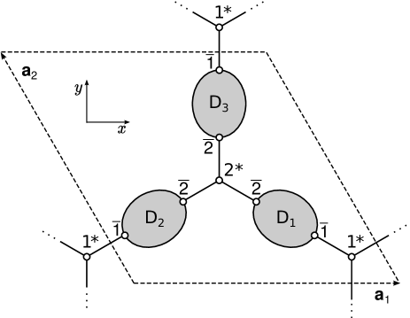
Figure 1: Primitive unit cell of bond-decorated graphene. $\mathbf{a}_{1}=(1,0)$, $\mathbf{a}_{2}=(-1/2,\sqrt{3}/2)$.

II.2 Bloch Hamiltonian

We describe the band structure by a Hückel Hamiltonian with on-site Coulomb energy $\alpha=0$ and transfer integral $\beta=1$. In this conventional setting the Hamiltonian is given by the adjacency matrix of the graph. Upon forming Bloch waves of the vertices the adjacency matrix factors into blocks labeled by wavevector $\mathbf{k}$:

$$\bm{\mathsf{H}}(\mathbf{k})=\begin{pmatrix}0&\gamma(\mathbf{k})&\mathbf{e}_{11}&e^{i\mathbf{k}\cdot\mathbf{a}_{1}}\mathbf{e}_{12}&e^{-i\mathbf{k}\cdot\mathbf{a}_{2}}\mathbf{e}_{13}\\ \overline{\gamma}(\mathbf{k})&0&\mathbf{e}_{21}&\mathbf{e}_{22}&\mathbf{e}_{23}\\ \mathbf{e}^{\intercal}_{11}&\mathbf{e}^{\intercal}_{21}&\bm{\mathsf{D}}_{1}&\bm{\mathsf{0}}&\bm{\mathsf{0}}\\ e^{-i\mathbf{k}\cdot\mathbf{a}_{1}}\mathbf{e}^{\intercal}_{12}&\mathbf{e}^{\intercal}_{22}&\bm{\mathsf{0}}&\bm{\mathsf{D}}_{2}&\bm{\mathsf{0}}\\ e^{i\mathbf{k}\cdot\mathbf{a}_{2}}\mathbf{e}^{\intercal}_{13}&\mathbf{e}^{\intercal}_{23}&\bm{\mathsf{0}}&\bm{\mathsf{0}}&\bm{\mathsf{D}}_{3}\end{pmatrix}$$ (1)

Here $\bm{\mathsf{D}}_{\kappa}$ are the adjacency matrices of the decorating fragments, and $\mathbf{e}_{1\kappa}$ and $\mathbf{e}_{2\kappa}$ are row vectors indicating which vertices of decoration $\kappa$ connect to the honeycomb vertices 1^∗ and 2^∗, respectively: $[\mathbf{e}_{1\kappa}]_{i}=\delta_{i\bar{1}}$ and $[\mathbf{e}_{2\kappa}]_{i}=\delta_{i\bar{2}}$. In expression (1) the first two rows/columns represent the vertices 1^∗ and 2^∗. The interaction element $\gamma$ can be expressed as

$$\gamma(\mathbf{k})=\delta_{1}+\delta_{2}e^{i\mathbf{k}\cdot\mathbf{a}_{1}}+\delta_{3}e^{-i\mathbf{k}\cdot\mathbf{a}_{2}},$$

where $\delta_{\kappa}=1$ if bond $\kappa$ is not decorated (i.e., if a direct edge connects 1^∗ and 2^∗ along bond $\kappa$), and 0 otherwise. Note that, in case bond $\kappa$ is not decorated, the columns and rows corresponding to $\bm{\mathsf{D}}_{\kappa}$ should be removed from $\bm{\mathsf{H}}$.

II.3 Effective two-band Hamiltonian

As we are interested in the presence of Dirac cones in the band spectrum, we shall be looking for discrete doubly degenerate zero-energy eigenvalues of the Bloch Hamiltonian $\bm{\mathsf{H}}(\mathbf{k})$. The approach followed here is to eliminate the bond decorations from the Hamiltonian, to obtain a low-energy two-band Hamiltonian on the honeycomb lattice with effective Coulomb and transfer integrals.

We write $\bm{\mathsf{H}}(\mathbf{k})$ in a compact notation as

$$\bm{\mathsf{H}}=\begin{pmatrix}\bm{\mathsf{H}}^{\ast}&\bm{\mathsf{T}}\\ \bm{\mathsf{T}}^{\dagger}&\bm{\mathsf{H}}_{\bm{\mathsf{D}}}\end{pmatrix}$$ (2)

and use the Schur complement formula (Ref. Horn1990, , 0.8.5, p. 21) to obtain a Löwdin partitioning of the secular determinant:

$$P(\mathbf{k},E)\equiv|E-\bm{\mathsf{H}}|=|E-\bm{\mathsf{H}}_{\bm{\mathsf{D}}}||E-\bm{\mathsf{H}}^{\ast}-\bm{\mathsf{T}}(E-\bm{\mathsf{H}}_{\bm{\mathsf{D}}})^{-1}\bm{\mathsf{T}}^{\dagger}|.$$ (3)

Introducing now the effective $2\times 2$ Hamiltonian on the honeycomb lattice

$$\widetilde{\bm{\mathsf{H}}^{\ast}}(E)=\bm{\mathsf{H}}^{\ast}+\bm{\mathsf{T}}(E-\bm{\mathsf{H}}_{\bm{\mathsf{D}}})^{-1}\bm{\mathsf{T}}^{\dagger}$$ (4)

and expanding $\bm{\mathsf{H}}_{\bm{\mathsf{D}}}$ gives

$$P(\mathbf{k},E)=|E-\bm{\mathsf{D}}_{1}||E-\bm{\mathsf{D}}_{2}||E-\bm{\mathsf{D}}_{3}||E-\widetilde{\bm{\mathsf{H}}^{\ast}}(E)|.$$ (5)

Zero-energy eigenvalues exist if the equation $P(\mathbf{k},0)=0$ has a solution. A problem arises when 0 is a root of one or more of the decorating units $\bm{\mathsf{D}}_{\kappa}$, for then the inverse of $\bm{\mathsf{H}}_{\bm{\mathsf{D}}}$ does not exist and the effective Hamiltonian is not defined at $E=0$, as can be seen from Eq. (4). However, as we will show below in Sec. II.3.1, this problem can be analyzed by factoring the dispersionless zero-energy poles out of each decoration’s Green’s function.

Let us now represent the effective Hamiltonian as follows, indicating explicitly its dependence on $\mathbf{k}$ and $E$ :

$$\widetilde{\bm{\mathsf{H}}^{\ast}}(\mathbf{k},E)=\begin{pmatrix}\alpha_{1}(E)&\Gamma(\mathbf{k},E)\\ \overline{\Gamma}(\mathbf{k},E)&\alpha_{2}(E)\end{pmatrix}$$ (6)

Define Green’s functions for the decorations:

$$\bm{\mathsf{G}}^{\kappa}(E)=(E-\bm{\mathsf{D}}_{\kappa})^{-1}=\frac{1}{|E-\bm{\mathsf{D}}_{\kappa}|}\operatorname{adj}(E-\bm{\mathsf{D}}_{\kappa}).$$ (7)

Then we find

$$\begin{split}\alpha_{1}(E)&=\bm{\mathsf{G}}^{1}_{\bar{1}\bar{1}}(E)+\bm{\mathsf{G}}^{2}_{\bar{1}\bar{1}}(E)+\bm{\mathsf{G}}^{3}_{\bar{1}\bar{1}}(E)\\ \alpha_{2}(E)&=\bm{\mathsf{G}}^{1}_{\bar{2}\bar{2}}(E)+\bm{\mathsf{G}}^{2}_{\bar{2}\bar{2}}(E)+\bm{\mathsf{G}}^{3}_{\bar{2}\bar{2}}(E)\\ \Gamma(\mathbf{k},E)&=\bm{\mathsf{G}}^{1}_{\bar{1}\bar{2}}(E)+e^{i\mathbf{k}\cdot\mathbf{a}_{1}}\bm{\mathsf{G}}^{2}_{\bar{1}\bar{2}}(E)+e^{-i\mathbf{k}\cdot\mathbf{a}_{2}}\bm{\mathsf{G}}^{3}_{\bar{1}\bar{2}}(E)\end{split}$$ (8)

The matrix elements in this expression follow from evaluation of Eq. (4): $\bm{\mathsf{G}}^{\kappa}_{\bar{i}\bar{j}}=\mathbf{e}_{i\kappa}\cdot\bm{\mathsf{G}}^{\kappa}\cdot\mathbf{e}_{j\kappa}^{\intercal}$. They represent the contribution from the decorations to the Coulomb integral on ($\alpha_{1}$ and $\alpha_{2}$) and the transfer/resonance integral between ($\Gamma$) the starred vertices of the honeycomb lattice.

Inspection of expression (6) learns that a pair of zero-energy solutions at wavevector $\mathbf{k}$ exists if and only if $\alpha_{1}(0)=\alpha_{2}(0)=0$ and $\Gamma(\mathbf{k},0)=0$.

II.3.1 Decorations with zero eigenvalues

Expressions Eq. (7) and Eq. (8) become ill-defined if the Hückel adjacency matrix $\bm{\mathsf{D}}_{\kappa}$ for one or more of the decorating graphs has zero eigenvalues. This case can be dealt with in some detail if the non-zero eigenvalues of the decorating graphs are known. For simplicity we discuss here the case of uniform decoration, where all three carbon–carbon bonds in the unit cell of graphene are decorated by the same chemical graph with $N$ vertices, having an adjacency matrix $\bm{\mathsf{D}}$ with $n<N$ zero eigenvalues (i.e. the decoration’s adjacency matrix has rank $m=N-n$) and $m$ non-zero eigenvalues $\lambda_{1},\dots,\lambda_{m}$. The analysis can be generalized to an arbitrary set of decorating graphs with an arbitrary number of zero eigenvalues, in a similar manner. We start off by writing an explicit expression for the decoration secular determinant in terms of its eigenvalues:

$$|E-\bm{\mathsf{D}}_{\kappa}|\equiv|E-\bm{\mathsf{D}}|=E^{n}|E-\bm{\mathsf{\tilde{D}}}|,$$ (9)

where $|E-\bm{\mathsf{\tilde{D}}}|$ is defined solely in terms of the $m$ non-zero eigenvalues as:

$$|E-\bm{\mathsf{\tilde{D}}}|=(E-\lambda_{1})(E-\lambda_{2})\dots(E-\lambda_{m}).$$ (10)

Using Eq. (9) to express the denominators in Eq. (7) and Eq. (8), the effective two-band Hamiltonian can now be written in a form that explicitly display its poles at $E=0$:

$$\begin{split}\widetilde{\bm{\mathsf{H}}^{\ast}}(\mathbf{k},E)&=\frac{1}{E^{n}}\sum_{\kappa=1,2,3}\bm{\mathsf{e}}_{\kappa}(\mathbf{k})\cdot\frac{\operatorname{adj}(E-\bm{\mathsf{D}})}{|E-\bm{\mathsf{\tilde{D}}}|}\cdot\bm{\mathsf{e}}_{\kappa}^{\intercal}(\mathbf{k})\\ &\equiv\frac{1}{E^{n}}\bm{\mathsf{M}}(\mathbf{k},E)\end{split}$$ (11)

If we label the two eigenvalues of the pole-free effective two-band Hamiltonian $\bm{\mathsf{M}}(E,\mathbf{k})$ introduced in Eq. (11) as $\eta_{1}(\mathbf{k},E)$ and $\eta_{2}(\mathbf{k},E)$, the secular polynomial for the decorated graphene can now be written as

$$P(\mathbf{k},E)=|E-\bm{\mathsf{\tilde{D}}}|^{3}\times E^{3n}\\ \times(E-\frac{\eta_{1}(\mathbf{k},E)}{E^{n}})\times(E-\frac{\eta_{2}(\mathbf{k},E)}{E^{n}}).$$ (12)

From Eq. (12) we can draw two conclusions.

First, as $E\rightarrow 0$, the denominator tends to zero as $E^{2n}$, while the numerator tends to zero as $E^{3n}$, which leads to a pole-free secular polynomial having a flat zero-energy band which is at least $n$-fold degenerate (in fact, for $n>1$, it can be seen that additional degeneracy of the flat zero-energy band arises from $\operatorname{adj}(E-\bm{\mathsf{D}})$).

Second and most important, by factoring out the poles of the singular effective Hamiltonian $\widetilde{\bm{\mathsf{H}}^{\ast}}(\mathbf{k},E)$ in this manner, we arrive at a reformulation of the secular polynomial of bond-decorated graphene where the problem of finding Dirac cones is reduced to the problem of finding the zero-energy solutions of a new non-singular effective two-band Hamiltonian $\bm{\mathsf{M}}(\mathbf{k},E)$ (see Eq. (11)), and is thus confined to the dispersion structure of the two eigenvalues $\eta_{1}(\mathbf{k},E)$ and $\eta_{2}(\mathbf{k},E)$. Necessary conditions for the existence of Dirac points can thus be derived in the same manner as for the case of bond-decorating graphs where the adjacency-rank is equal to the number of vertices (see Eq. (8) and the following discussion).

II.4 Criteria for the existence of Dirac points

In order to simplify expressions in the discussions that follow we introduce the notation of Pickup and FowlerPickup2008 for the polynomials that appear in Eqs. (7) and (8):

$$\begin{split}s_{\kappa}(E)&=|E-\bm{\mathsf{D}}_{\kappa}|\\ t_{\kappa}(E)&=|(E-\bm{\mathsf{D}}_{\kappa})^{\bar{1},\bar{1}}|\\ u_{\kappa}(E)&=|(E-\bm{\mathsf{D}}_{\kappa})^{\bar{2},\bar{2}}|\\ v_{\kappa}(E)&=|(E-\bm{\mathsf{D}}_{\kappa})^{\bar{1}\bar{2},\bar{1}\bar{2}}|\\ w_{\kappa}(E)&=(-1)^{\bar{1}+\bar{2}}|(E-\bm{\mathsf{D}}_{\kappa})^{\bar{2},\bar{1}}|,\end{split}$$ (13)

where $\bm{\mathsf{M}}^{i_{1}i_{2}\ldots,j_{1}j_{2}\ldots}$ is the matrix derived from $\bm{\mathsf{M}}$ by removing rows $i_{1},i_{2},\ldots$ and columns $j_{1},j_{2},\ldots$. The polynomials in Eq. (13) are related by the Sylvester identity for determinants (See Appendix 2 in Ref. Gutman1986, ), which reads

$$t_{\kappa}u_{\kappa}-s_{\kappa}v_{\kappa}=w_{\kappa}^{2}.$$ (14)

Eq. (8) can now be written as

$$\begin{split}\alpha_{1}&=\frac{t_{1}}{s_{1}}+\frac{t_{2}}{s_{2}}+\frac{t_{3}}{s_{3}}\\ \alpha_{2}&=\frac{u_{1}}{s_{1}}+\frac{u_{2}}{s_{2}}+\frac{u_{3}}{s_{3}}\\ \Gamma&=\frac{w_{1}}{s_{1}}+e^{i\theta_{1}}\frac{w_{2}}{s_{2}}+e^{-i\theta_{2}}\frac{w_{3}}{s_{3}},\end{split}$$ (15)

where $\theta_{i}=\mathbf{k}\cdot\mathbf{a}_{i}$.

A spectrum with Dirac cones is characterized by a discrete number of wavevectors at which two bands cross linearly with energy equal to zero (this is the Fermi energy). These wavevectors are called Dirac points in the Brillouin zone. For simplicity we restrict attention to decorations that have no zero eigenvalues. This means that $s_{\kappa}\neq 0$ at $E=0$ for all $\kappa$. Then, as seen before, Dirac points are solutions of the equations $\alpha_{1}(0)=\alpha_{2}(0)=0$ and $\Gamma(\mathbf{k},0)=0$. Note that only the last equation determines, implicitly, the position of the Dirac points, if any. The first two equations are wavevector-independent. They read, according to Eq. (15),

$$\begin{split}\frac{t_{1}}{s_{1}}+\frac{t_{2}}{s_{2}}+\frac{t_{3}}{s_{3}}&=0\quad\text{at }E=0\\ \frac{u_{1}}{s_{1}}+\frac{u_{2}}{s_{2}}+\frac{u_{3}}{s_{3}}&=0\quad\text{at }E=0.\end{split}$$ (16)

The equations can be satisfied by an accidental cancellation of terms, but more relevant are cases in which the terms vanish individually, i.e. $t_{1}=t_{2}=t_{3}=0$ at $E=0$, and $u_{1}=u_{2}=u_{3}=0$ at $E=0$. In the rest of the paper we shall be considering only this case.

In terms of graph theory we know that $s_{\kappa}$ is the characteristic polynomial of the graph of decoration $\kappa$. From Eq. (13) $t_{\kappa}$ is seen to be the characteristic polynomial of a subgraph of $\kappa$, namely the subgraph obtained by removing vertex $\bar{1}$, which is the one that connects to vertex $1^{\ast}$ of the honeycomb lattice.Pickup2008 Similarly, $u_{\kappa}$ is the characteristic polynomial of the graph $\kappa$ with vertex $\bar{2}$ removed. Note that $\bar{1}$ and $\bar{2}$ can be the same vertex. In that case $u_{\kappa}=t_{\kappa}$.

From the preceding discussion we conclude that the first condition for the presence of Dirac points, expressed in Eq. (16), is a condition on zeros in the spectrum of the decorating graphs and subgraphs. This condition states that none of the three decorating graphs can have nonbonding orbitals while each of the six single-vertex-deleted subgraphs must have a nonbonding orbital.

The second condition states that the off-diagonal element in the effective two-band Hamiltonian (6) is zero at the Fermi energy $E=0$. From Eq. (15), this means

$$\Gamma(\mathbf{k},0)\equiv\frac{w_{1}}{s_{1}}+e^{i\theta_{1}}\frac{w_{2}}{s_{2}}+e^{-i\theta_{2}}\frac{w_{3}}{s_{3}}=0\quad\text{at }E=0.$$

We note that $\Gamma(\mathbf{k},0)$ can be seen as the off-diagonal element in the two-band tight binding model of the anisotropic honeycomb lattice Hasegawa2006 if we identify the hopping integrals $\beta_{\kappa}$ of the latter with the polynomial ratios in our expression: $\beta_{\kappa}\equiv\frac{w_{\kappa}}{s_{\kappa}}|_{E=0}$. The off-diagonal condition can then be written as

$$\beta_{1}+e^{i\theta_{1}}\beta_{2}+e^{-i\theta_{2}}\beta_{3}=0.$$ (17)

Solving this equation for $(\theta_{1},\theta_{2})$ gives the positions in the Brillouin zone where two bands are degenerate at $E=0$ (assuming that the conditions Eq. (16) on the diagonal elements are also fulfilled). Given that the $\beta_{\kappa}$ are all real, Eq. (17) describes a triangle in the complex plane, with sides of length $|\beta_{1}|$, $|\beta_{2}|$, and $|\beta_{3}|$. Hence a solution to Eq. (17) exists only when the effective hopping parameters satisfy the triangle inequality Hasegawa2006 ; Kim2012

$$(|\beta_{1}|-|\beta_{2}|)^{2}\leq|\beta_{3}|^{2}\leq(|\beta_{1}|+|\beta_{2}|)^{2}.$$ (18)

In order to have a discrete number of Dirac points we must also require that none of the $\beta_{\kappa}$ be zero. Consider the two possibilities: (i) $\beta_{1}=\beta_{2}=\beta_{3}=0$. Then Eq. (17) is automatically satisfied over the entire Brillouin zone, which means that there are two flat bands at $E=0$ but no Dirac cones; (ii) $\beta_{1}=0$ and $|\beta_{2}|=|\beta_{3}|$, or a circular permutation of this. Then solution of Eq. (17) gives a one-dimensional domain in the Brillouin zone (namely, straight line(s)), in which two bands are degenerate at $E=0$. In both cases (i) and (ii) isolated Dirac points do not exist. If, then, none of the $\beta_{\kappa}$ is zero and the triangle inequality (18) is satisfied, there are just two solutions to Eq. (17) and hence two Dirac points. These solutions are related by time reversal: $(\theta_{1},\theta_{2})\leftrightarrow(-\theta_{1},-\theta_{2})$.

Let us now see what $\beta_{\kappa}\equiv\frac{w_{\kappa}}{s_{\kappa}}|_{E=0}\neq 0$ means in terms of the spectral properties of the decoration. The definition of $w_{\kappa}$ in Eq. (13) shows that $w_{\kappa}$ is not the characteristic polynomial of some graph derived from the graph of $\kappa$. It is, however, related to such polynomials via the Sylvester identity Eq. (14). Recall from the discussion preceding and following Eq. (16) that we are considering decorations for which $s_{\kappa}\neq 0$ at $E=0$ and $t_{\kappa}=u_{\kappa}=0$ at $E=0$. Then Eq. (14) tells us that $w_{\kappa}^{2}|_{E=0}=s_{\kappa}v_{\kappa}|_{E=0}$, implying that $w_{\kappa}$, and thus $\beta_{\kappa}$, is non-zero at $E=0$ when $v_{\kappa}$ is non-zero at $E=0$. $v_{\kappa}$ is the characteristic polynomial of the graph of decoration $\kappa$ with vertices $\bar{1}$ and $\bar{2}$ removed.Pickup2008 Hence we conclude that $\beta_{\kappa}$ is non-zero iff the $(\bar{1},\bar{2})$-vertex-deleted subgraph of decoration $\kappa$ has no non-bonding orbitals.

In summary, discrete Dirac points in the spectrum of bond-decorated graphene exist if all of the following statements about the spectral properties of the three decorating graphs are true:

1. None of the three decorating graphs has non-bonding orbitals.

2. Each of the six subgraphs obtained by deleting the contacting vertices $\bar{1}$ or $\bar{2}$ has at least one non-bonding orbital.

3. None of the three subgraphs obtained by deleting both contacting vertices $\bar{1}$ and $\bar{2}$ has non-bonding orbitals.

4. $(|\beta_{1}|-|\beta_{2}|)^{2}\leq|\beta_{3}|^{2}\leq(|\beta_{1}|+|\beta_{2}|)^{2}$, where $\beta_{\kappa}=\frac{w_{\kappa}}{s_{\kappa}}|_{E=0}$.

III Example: Chlorinated graphene

Chemically functionalized graphenes are systems where the findings of this paper can apply. We want to illustrate this with the example of a chlorinated graphene sheet whose stoichiometry is C₄Cl. The chlorine atoms in this compound form single covalent bonds with carbon atoms of the graphene sheet. The C–Cl bonds are arranged in a periodical pattern (i.e., translationally symmetric) and are distributed such that half of the chlorine atoms are found on one side of the graphene plane and the other half on the other side (see Fig. 2). In a DFT study, this compound was found to be the most stable one among double-sided chlorinated graphenes.Yang2012 Its experimental realization was reported recently.Zhang2013

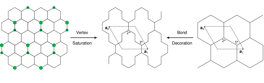
Figure 2: Chlorination pattern of C₄Cl chlorinated graphene (left). Chlorinated carbon atoms, which are sp³ hybridized and do not contribute to the conjugated $\pi$ electron system, are deleted to obtain the Hückel graph (middle). The latter can be derived formally from graphene by decorating two of the three bonds in the unit cell with ethylene (right $\rightarrow$ middle).

From the point of view of electronic structure the effect of the covalent bonding to chlorine is to change the hybridization of the carbon atom from sp² to sp³. The sp³ carbon atoms do not contribute to the $\pi$-electron structure and may therefore be discarded. What remains is a network of sp² carbon atoms whose band structure can be determined, in first approximation, with Hückel theory. Fig. 2 shows how the sp² network is obtained for the C₄Cl example under consideration. It is apparent from Fig. 2 that the network can be interpreted as a decorated graphene lattice in the sense of this paper. Two bonds are decorated with an “ethylene” unit. The third bond is not decorated. Hence $\gamma(\mathbf{k})=e^{-i\mathbf{k}\cdot\mathbf{a}_{2}}$ and

$$\bm{\mathsf{D}}_{1}=\bm{\mathsf{D}}_{2}=\begin{pmatrix}0&1\\ 1&0\end{pmatrix}.$$ (19)

Table 1: Polynomials defined in Eq. (13), calculated for the C₄Cl system depicted in Fig. 2.

Decoration	$s$	$t$	$u$	$v$	$w$
1	$E^{2}-1$	$E$	$E$	1	$1$
2	$E^{2}-1$	$E$	$E$	1	$1$
3	$1$	$0$	$0$	$-1$	$1$
	$s(0)$	$t(0)$	$u(0)$	$v(0)$	$w(0)$
1	$-1$	$0$	$0$	1	$1$
2	$-1$	$0$	$0$	1	$1$
3	$1$	$0$	$0$	$-1$	$1$

Table 1 collects the different polynomials that characterize the decorations. For the undecorated bond (nr 3) we have chosen values for these polynomials that are consistent with Eq. (14) and that can be used in equations like Eq. (16). This allows us to treat all three bonds on equal footing in the discussion that follows.

To determine whether Dirac points exist we need to inspect the values of the polynomials at $E=0$. These are given in the bottom half of Table 1. It is straightforward to check that the first three of the four conditions formulated at the end of Section 2 hold: For each of the three decorations, $s(0)$ is non-zero, $t(0)$ and $u(0)$ are zero, and $v(0)$ is non-zero. To check the fourth condition we first compute the effective hopping integrals $\beta_{\kappa}=\frac{w_{\kappa}(0)}{s_{\kappa}(0)}$, giving $\beta_{1}=\beta_{2}=-1$ and $\beta_{3}=1$. These satisfy the triangle inequality, and therefore the fourth condition is also satisfied. We conclude that the Hückel band spectrum of CCl₄ has two Dirac points.

The positions of the Dirac points in the Brillouin zone are obtained from Eq. (17), which reads

$$-1-e^{i\theta_{1}}+e^{-i\theta_{2}}=0.$$

This equation has two solutions: $(\theta_{1},\theta_{2})=(2\pi/3,-\pi/3)$ and $(\theta_{1},\theta_{2})=(-2\pi/3,\pi/3)$. Recalling that $\theta_{i}=\mathbf{k}\cdot\mathbf{a}_{i}$, we find that the Dirac points are located at the wavevectors $\mathbf{k}=(2\pi/3,0)$ and $\mathbf{k}=(-2\pi/3,0)$.

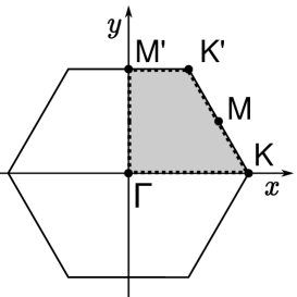
	$(x,y)$
$\Gamma$	$(0,0)$
K	$(\frac{2}{3},0)$
M	$(\frac{1}{2},\frac{1}{2\sqrt{3}})$
K’	$(\frac{1}{3},\frac{1}{\sqrt{3}})$
M’	$(0,\frac{1}{\sqrt{3}})$

Figure 3: Brillouin zone for the C₄Cl Hückel system depicted in Fig. 2. The symmetry-unique basic domain (grey area) is defined by the $D_{\mathrm{2h}}$ point group symmetry of the Hückel graph. The dashed line indicates the path along which the band energies are plotted in Fig. 4. The coordinates in the table are in units of $2\pi$.

III.1 Analytical solution of the Hückel band spectrum

Although the Bloch Hamiltonian for the the CCl₄ Hückel graph is a $6\times 6$ matrix, closed-form expressions for its eigenvalues can be obtained. This is due to the matrix being bipartite, which means that its rows/columns can be divided in two groups such that all the matrix elements that connect one group to the other vanish. When the two groups are of equal size (as is the case for the current example), it is known that the energies occur in pairs of opposite sign.Coulson1940 It follows that the energies squared are the roots of a cubic polynomial.

The Bloch Hamiltonian for the CCl₄ Hückel problem is given by Eq. (1) with $\gamma(\mathbf{k})=e^{-i\theta_{2}}$, $\mathbf{e}_{11}=(1\;0)=\mathbf{e}_{12}$, $\mathbf{e}_{21}=(0\;1)=\mathbf{e}_{22}$, and $\bm{\mathsf{D}}_{1}$ and $\bm{\mathsf{D}}_{2}$ as in Eq. (19). The entries in Eq. (1) that refer to bond 3 are omitted as this bond is not decorated.

$$\bm{\mathsf{H}}(\mathbf{k})=\begin{pmatrix}0&e^{-i\theta_{2}}&1&0&e^{i\theta_{1}}&0\\ e^{i\theta_{2}}&0&0&1&0&1\\ 1&0&0&1&0&0\\ 0&1&1&0&0&0\\ e^{-i\theta_{1}}&0&0&0&0&1\\ 0&1&0&0&1&0\\ \end{pmatrix}.$$

Collecting rows/columns 1, 4, and 6 in group $A$ and 2, 3, and 5 in group $B$ and rearranging the matrix accordingly clarifies its bipartite structure:

$$\begin{split}&\bm{\mathsf{H}}(\mathbf{k})=\begin{pmatrix}\bm{\mathsf{0}}&\bm{\mathsf{H}}_{AB}(\mathbf{k})\\ \bm{\mathsf{H}}_{AB}^{\dagger}(\mathbf{k})&\bm{\mathsf{0}}\end{pmatrix},\\ &\bm{\mathsf{H}}_{AB}(\mathbf{k})=\begin{pmatrix}e^{-i\theta_{2}}&1&e^{i\theta_{1}}\\ 1&1&0\\ 1&0&1\end{pmatrix}\end{split}$$ (20)

The characteristic polynomial can be found, for example, by use of Schur’s formula (Eqs. (2) and (3)). This gives

$$P(\mathbf{k},E)=|E^{2}-\bm{\mathsf{H}}_{AB}\bm{\mathsf{H}}_{AB}^{\dagger}|.$$

$E^{2}$, therefore, is an eigenvalue of the $3\times 3$ matrix $\bm{\mathsf{H}}_{AB}\bm{\mathsf{H}}_{AB}^{\dagger}$. The latter is readily computed from Eq. (20):

$$\begin{split}\bm{\mathsf{H}}_{AB}\bm{\mathsf{H}}_{AB}^{\dagger}&=\frac{7}{3}+\begin{pmatrix}\frac{2}{3}&1+e^{-i\theta_{2}}&e^{i\theta_{1}}+e^{-i\theta_{2}}\\ 1+e^{i\theta_{2}}&-\frac{1}{3}&1\\ e^{-i\theta_{1}}+e^{i\theta_{2}}&1&-\frac{1}{3}\end{pmatrix}\\ &\equiv\frac{7}{3}+\bm{\mathsf{N}}\end{split}$$

The eigenvalues of the traceless, Hermitian matrix $\bm{\mathsf{N}}$ can be conveniently expressed as

$$\lambda_{n}=\rho\cos(\phi+n\frac{2\pi}{3}),\quad n=0,1,2,$$

with

$$\begin{split}\rho^{2}&=\frac{2}{3}\operatorname{Tr}(\bm{\mathsf{N}}^{2})=\frac{8}{3}\left[\frac{8}{3}+\cos\theta_{2}+\cos(\theta_{1}+\theta_{2})\right],\\ \cos(3\phi)&=\frac{4}{\rho^{3}}|\bm{\mathsf{N}}|\\ &=\frac{4}{\rho^{3}}\left[\frac{74}{27}+\frac{8}{3}\Bigl{(}\cos\theta_{2}+\cos(\theta_{1}+\theta_{2})\Bigr{)}+2\cos\theta_{1}\right].\end{split}$$

Now switching to cartesian coordinates of reciprocal space by substituting $\theta_{i}=\mathbf{k}\cdot\mathbf{a}_{i}$, we find

$$\begin{split}\rho&=\frac{4}{3}\sqrt{4+3\cos\frac{k_{x}}{2}\cos\frac{\sqrt{3}k_{y}}{2}},\\ |\bm{\mathsf{N}}|&=\frac{4}{3}\left[\frac{5}{9}+\cos\frac{k_{x}}{2}\left(3\cos\frac{k_{x}}{2}+4\cos\frac{\sqrt{3}k_{y}}{2}\right)\right].\end{split}$$

With these expressions the complete solution for the six band energies is obtained in closed form: $E=\pm\sqrt{7/3+\lambda_{n}}$, or

$$E=\pm\sqrt{\frac{7}{3}+\rho\cos\left(\frac{1}{3}\arccos\frac{4|\bm{\mathsf{N}}|}{\rho^{3}}+n\frac{2\pi}{3}\right)},\quad n=0,1,2.$$ (21)

With the exact solution at hand it is now possible to check that there are indeed two Dirac points and that they are located at $\mathbf{k}=\pm(2\pi/3,0)$, as found above. A Taylor expansion of Eq. (21) shows that the energy in the neighborhood of the Dirac points is given by the isotropic dispersion

$$E=\pm\frac{1}{2\sqrt{3}}\sqrt{\xi^{2}+\eta^{2}},$$

where $\xi$ and $\eta$ are the displacement of $k_{x}$ and $k_{y}$ from the Dirac point. This proves the presence of two isotropic Dirac cones. A plot of Eq. (21) over the entire Brillouin zone (not shown) reveals no other Dirac cones.

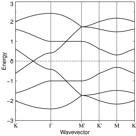
Figure 4: The Hückel band energies, Eq. (21), are plotted along the boundary of the basic domain, see Fig. 3. A Dirac cone appears exactly halfway between $\Gamma$ and K.

- (1) A. H. Castro Neto, F. Guinea, N. M. R. Peres, K. S. Novoselov, and A. K. Geim, Rev. Mod. Phys. 81, 109 (2009).
- (2) K. S. Novoselov, A. K. Geim, S. V. Morozov, D. Jiang, M. I. Katsnelson, I. V. Grigorieva, S. V. Dubonos, and A. A. Firsov, Nature 438, 197 (2005).
- (3) M. I. Katsnelson, K. S. Novoselov, and A. K. Geim, Nature Phys. 2, 620 (2006).
- (4) B. G. Kim and H. J. Choi, Phys. Rev. B 86, 115435 (2012).
- (5) J.-J. Zheng, X. Zhao, S. B. Zhang, and X. Gao, J. Chem. Phys. 138, 244708 (2013).
- (6) F. Ouyang, S. Peng, Z. Liu, and Z. Liu, ACS Nano 5, 4023 (2011).
- (7) M. Yang, L. Zhou, J. Wang, Z. Liu, and Z. Liu, J. Phys. Chem. C 116, 844 (2012).
- (8) L. Zhang, J. Yu, M. Yang, Q. Xie, H. Peng, and Z. Liu, Nat. Commun. 4, 1443 (2013).
- (9) Y. Ma, Y. Dai, and B. Huang, J. Phys. Chem. Lett. 4, 2471 (2013).
- (10) A. Soncini, P. W. Fowler, I. Cernusak, and E. Steiner, Phys. Chem. Chem. Phys. 3, 3920 (2001).
- (11) A. Soncini, P. W. Fowler, and L. W. Jenneskens, Struc. Bond. 115, 57 (2005).
- (12) A. Soncini, C. Domene, J. J. Engelberts, P. W. Fowler, A. Rassat, J. H. van Lenthe, R. W. A. Havenith, and L. W. Jenneskens, Chem. Eur. J. 11, 1257 (2005).
- (13) P. W. Fowler, R. W. A. Havenith, L. W. Jenneskens, A. Soncini, and E. Steiner, Chem. Commun., 2386(2001).
- (14) A. Soncini, R. W. A. Havenith, P. W. Fowler, L. W. Jenneskens, and E. Steiner, J. Org. Chem. 67, 4753 (2002).
- (15) R. A. Horn and C. R. Johnson, Matrix analysis (Cambridge University Press, 1990).
- (16) Assuming for now that all three bonds are decorated, so that . This is done for generality only; it does not represent a limitation of the theory. The example in Sec. III will show how to treat undecorated bonds on the same footing as decorated bonds.
- (17) B. T. Pickup and P. W. Fowler, Chem. Phys. Lett. 459, 198 (2008).
- (18) I. Gutman and O. E. Polansky, Mathematical concepts in organic chemistry (Springer, Berlin, 1986).
- (19) Y. Hasegawa, R. Konno, H. Nakano, and M. Kohmoto, Phys. Rev. B 74, 033413 (2006).
- (20) C. A. Coulson and G. S. Rushbrooke, Proc. Camb. Phil. Soc. 36, 193 (1940).