The Hantzsche-Wendt Manifold in Cosmic Topology

Abstract

The Hantzsche-Wendt space is one of the 17 multiply connected spaces of the three-dimensional Euclidean space $\mathbb{E}^{3}$. It is a compact and orientable manifold which can serve as a model for a spatial finite universe. Since it possesses much fewer matched back-to-back circle pairs on the cosmic microwave background (CMB) sky than the other compact flat spaces, it can escape the detection by a search for matched circle pairs. The suppression of temperature correlations $C(\vartheta)$ on large angular scales on the CMB sky is studied. It is shown that the large-scale correlations are of the same order as for the 3-torus topology but express a much larger variability. The Hantzsche-Wendt manifold provides a topological possibility with reduced large-angle correlations that can hide from searches for matched back-to-back circle pairs.

1 Introduction

An interesting aspect of cosmology concerns the global spatial structure of our Universe, that is the question for its topology. For review papers of cosmic topology and for discussions concerning topological tests, see [1, 2, 3, 4, 5, 6, 7, 8]. Since the standard $\Lambda$CDM concordance model of cosmology is based on the spatial flat space, the topological question might be restricted to space forms admissible in the three-dimensional Euclidean space $\mathbb{E}^{3}$. There are 18 possible space forms which are denoted as $E_{1}$ to $E_{18}$ in [1, 9, 8]. The space $E_{18}$ is the usual simply connected Euclidean space without compact directions. The remaining 17 space forms possess compact directions and are thus multiply connected. The usual three-dimensional Euclidean space $\mathbb{E}^{3}$ can be considered as their universal cover which is tessellated by the multiply connected space forms into spatial domains which have to be identified. Eight of the 17 space forms are non-orientable manifolds which are usually not taken into account in cosmology. Thus there are 9 orientable multiply connected manifolds and 6 of them are compact. The focus is usually put on the 6 compact space forms $E_{1}$ to $E_{6}$. From these the 3-torus topology $E_{1}$ has attracted the most attention and its cosmological implications are well understood. The $E_{1}$ space has the simplifying property that the statistical cosmological properties are independent of the position of the observer for which the statistics, e. g. of the cosmic microwave background (CMB) radiation, is computed. This simplification is not possible for the other compact orientable multiply connected manifolds $E_{2}$ to $E_{6}$ and the statistics of the CMB simulations, on which the focus is put in this paper, have to be computed for a sufficiently large number of observer positions on the manifold in order to obtain a representative result for such an inhomogeneous manifold.

A method to detect a non-trivial topology of our Universe is the search for the circles-in-the-sky (CITS) signature [10]. Since the space is multiply connected, the sphere from which the CMB radiation is emitted towards a given observer can overlap with another sphere belonging to a position in the universal cover which is, due to the topology, to be identified with that of the considered observer. The intersection of such spheres leads to circles on the CMB sky where the temperature fluctuations are correlated according to the assumed topology. The simplest situation is realised by two circles whose centres are antipodal on the CMB sky. Such circle pairs are called “back-to-back”. This is the type of matched circle pairs which is the easiest one to discover in CMB sky maps. The non-back-to-back matched circle pairs have two further degrees of freedom due to the position of the centre of the second circle. This significantly enlarges the numerical effort in the CMB analysis and, in addition, increases the background of accidental correlations which can swamp the true signal of a matched circle pair. There are a lot of papers devoted to the CITS search [11, 12, 13, 14, 15, 16, 17, 18, 19, 20, 21, 22, 23]. The result is that there is no convincing hint for a matched back-to-back circle pair in the CMB data with a radius above $25^{\circ}\dots 30^{\circ}$. Smaller back-to-back circle pairs are not detectable [22]. This leads to the question whether space forms without back-to-back circle pairs can get missed by these searches. The non-back-to-back circle search in [20] does not find hints of such a topology. However, it is shown in [22] that the search grid in [20] is too coarse such that even large back-to-back circles with radii up to $50^{\circ}$ are not found (see figure 4 in [22]). The analysis in [22] refers to back-to-back circle pairs, but the increased background in the general case worsen the detectability of non-back-to-back circles. Furthermore, due to foreground contamination in two regions of the CMB map, the search in [20] excludes circles which intersect these regions. Thus it is safe to say that [20] does not find a hint in favour of such a topology, but it cannot exclude one.

Restricting to the Euclidean case with its 6 compact orientable space forms, one can ask which topology does not possess back-to-back circle pairs with radii above $25^{\circ}\dots 30^{\circ}$. The answer depends on the value of the parameters $L_{i}$, which define the size and shape of the Dirichlet cell, see equation (1) below. Let us assume that these parameters are chosen in such a way that all spatial dimensions of the Dirichlet cell are of the same order. This ensures that the largest circle pairs arise from the identification of the faces of the Dirichlet cell. The topologies $E_{1}$ to $E_{5}$ identify at least two pairs of faces by pure translations, i. e. without an accompanying rotation. These translations lead to back-to-back circle pairs for all observer positions even in the case of an inhomogeneous manifold. For example, the spaces $E_{4}$ and $E_{5}$, belonging to a hexagonal tiling of the Euclidean space, possess three back-to-back circle pairs due to the three pairs of faces that are identified by pure translations. In this respect, the manifold $E_{6}$ is special since every identification of a pair of faces is defined by a translation and a rotation by $\pi$, i. e. a so-called half-turn corkscrew motion. The space form $E_{6}$ is also called Hantzsche-Wendt space [24] and is the topic of this paper.

Therefore, the Hantzsche-Wendt space is a candidate for cosmic topology worth studying its implications on the CMB sky. The CMB angular power spectrum is computed for a single observer position in [25] for low multipoles, and a suppression of temperature correlations on large angular scales is found. Besides this, there are no further CMB analyses in literature, although [9] describes the eigenmodes of that space form allowing the computation of CMB fluctuations for an observer at the origin of the coordinate system. The aim of this paper is to provide a CMB analysis of the temperature correlations on large angular scales for a huge sample of observer positions in order to allow a comparison with the CMB observations.

2 Hantzsche-Wendt Topology

The Hantzsche-Wendt manifold $\mathbb{E}^{3}/\Gamma$ is the quotient of the Euclidean space $\mathbb{E}^{3}$ by the holonomy group $\Gamma$ which is generated by the transformations

$$(\tilde{x},\tilde{y},\tilde{z}) \rightarrow (\tilde{x}+L_{x},-\tilde{y},-\tilde{z})$$

$$(\tilde{x},\tilde{y},\tilde{z}) \rightarrow (-\tilde{x},\tilde{y}+L_{y},-(\tilde{z}+L_{z}))$$ (1)

$$(\tilde{x},\tilde{y},\tilde{z}) \rightarrow (-(\tilde{x}+L_{x}),-(\tilde{y}+L_{y}),\tilde{z}+L_{z})$$

with the topological scale defining parameters $L_{x}$, $L_{y}$, and $L_{z}$. These generators are half-turn corkscrew motions, since each transformation contains a rotation by $\pi$, and lead to a fixed point free symmetry group $\Gamma$. The definition (1) of the generators of $\Gamma$ agrees with that in [26, 25] but, however, differs from that in [9, 8]. The various definitions of the generators of $\Gamma$ all lead to the same manifold, of course, but correspond to different positions on the manifold which are taken as the origin of the reference system. It is convenient to describe the positions $\vec{x}$ by dimensionless coordinates $x$, $y$, $z\in[-0.5,0.5]$, such that a position $(x,y,z)$ with $\vec{x}:=(xL_{x},yL_{y},zL_{z})$ refers to corresponding positions in Hantzsche-Wendt spaces defined by different sets of topological length scales. The Dirichlet domain with respect to a position $\vec{x}_{o}$ is defined as the set of points $\vec{x}$ such that $d(\vec{x}_{o},\vec{x})\leq d(\vec{x}_{o},\gamma\vec{x})$ $\forall\gamma\in\Gamma$. Figure 1 shows four examples of the Dirichlet domain based on the generators (1). The geometrical shape of the Dirichlet domain possesses only for special chosen positions $(x,y,z)$ highly symmetrical domains, e. g. a cuboid for $(0,0,0)$ or a rhombic dodecahedron for $(0,\frac{1}{2},0)$ for $L_{x}=L_{y}=L_{z}$.

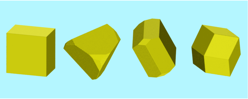
Figure 1: The Dirichlet domain is shown for four different observer positions, i. e. different positions on the manifold taken as the origin of the reference system. The topological parameters are set equal, i. e. $L_{x}=L_{y}=L_{z}$. The positions are indicated in the figure by the relative positions $(x,y,z)$. While for $(x,y,z)=(0,0,0)$ the Dirichlet domain is a cuboid, a rhombic dodecahedron is obtained for $(x,y,z)=\left(0,\frac{1}{2},0\right)$.

At a first sight, one might get the impression that the domains shown in figure 1(b) or 1(c) might not tessellate the Euclidean space. To demonstrate that this is indeed the case, figure 2 shows for the case $(x,y,z)=\left(\frac{1}{4},\frac{1}{4},\frac{1}{4}\right)$, i. e. figure 1(b), how four adjacent Dirichlet domains stick together according to the group $\Gamma$ generated by (1). One interesting corner of the Dirichlet domain is indicated by the arrow in figure 2, which is formed by three small surface patches. This surface structure matches the joint of the three Dirichlet domains shown in the centre of figure 2. In this way, the next Dirichlet domain would exactly match to this dip, so that the Euclidean space is tessellated with no overlaps and no gaps.

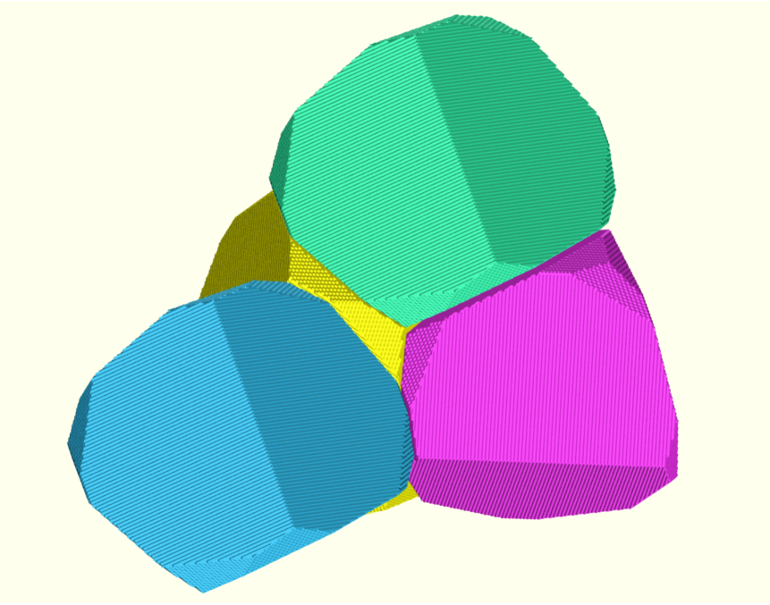
Figure 2: The Dirichlet domain is shown for the observer position $(x,y,z)=\left(\frac{1}{4},\frac{1}{4},\frac{1}{4}\right)$ with three adjacent domains. The arrow points towards a corner on the Dirichlet domain, where three small patches meet. This corner fits into the region shown in the centre of the image, where the yellow, green and purple domains are in direct contact.

Another possibility to obtain information about the shape of the Dirichlet domain is to consider the range of distances $r$ of the observer positions from the surface of the Dirichlet domain. In figure 3 the values of the minimum of these distances $r_{\hbox{\scriptsize min}}$ and of the maximum $r_{\hbox{\scriptsize max}}$ are plotted for two sets of observer positions. Panel 3(a) shows the distances for the line parameterised as $(x,y,z)=(t,t,t)$, $t\in[0,1]$, which for $t=0$ and $t=\frac{1}{4}$ agrees with the observer positions of figures 1(a) and 1(b). One observes that for $t=0$ the width of the distribution of the distances is maximal that is $r_{\hbox{\scriptsize min}}$ is minimal and $r_{\hbox{\scriptsize max}}$ is maximal. The reverse situation occurs for $t=\frac{1}{4}$ where the width is minimal. Figure 3(b) shows the distances for the line $(x,y,z)=(0,t,0)$, where the example for $t=\frac{1}{2}$ is displayed in figure 1(d). This position belongs to the rhombic dodecahedron having a minimal width $r_{\hbox{\scriptsize max}}-r_{\hbox{\scriptsize min}}$ as figure 3(b) reveals.

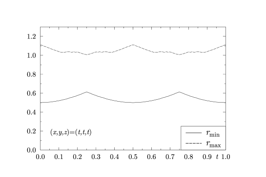
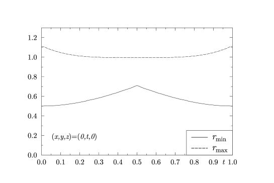
Figure 3: The distance to the surface of the Dirichlet domain measured from the observer position is shown. The minimal distance is plotted as $r_{\hbox{\scriptsize min}}$ and the maximal distance as $r_{\hbox{\scriptsize max}}$. The position of the observer is varied along the line $(x,y,z)=(t,t,t)$ in panel (a) and along $(x,y,z)=(0,t,0)$ in panel (b) for $t\in[0,1]$. The topological parameters are set as $L_{x}=L_{y}=L_{z}=1$.

In the following, we will measure $L_{x}$, $L_{y}$, and $L_{z}$ in units of the Hubble length $L_{\hbox{\scriptsize H}}=c/H_{0}$. The parameters of the $\Lambda$CDM concordance model used in this paper are obtained from Table 8, column “WMAP+BAO+$H_{0}$” of [27] stating the values $\Omega_{\hbox{\scriptsize bar}}=0.0456$, $\Omega_{\hbox{\scriptsize cdm}}=0.227$, a present day reduced Hubble constant $h=0.704$, a reionization optical depth $\tau=0.087$, and a scalar spectral index $n_{s}=0.963$. These parameters lead to a diameter of the surface of last scattering of $D_{\hbox{\scriptsize sls}}=6.605$ in units of $L_{\hbox{\scriptsize H}}\simeq 4.258\hbox{ Gpc}$. The order of the topological length scale should not significantly be above $D_{\hbox{\scriptsize sls}}$ in order to leave a signature on the CMB sky [28]. Although the cosmological parameters of $\Lambda$CDM concordance model differ for the different WMAP data releases and also depend on the inclusions of other cosmological observations, it is not expected that the topological results referring to the largest scales are affected by these changes. This statement also applies to the parameter set given by the Planck collaboration [29].

The fact that all three generators are half-turn corkscrew motions leads to the important consequence that the matched circles pairs with the largest radii are not of the back-to-back type. The difficulties in detecting such matched circles pairs motivate the CMB analysis of the Hantzsche-Wendt space as discussed in the Introduction. Let us now discuss how many matched back-to-back circle pairs exist for a given Hantzsche-Wendt manifold on the corresponding CMB sky. Although, for general observer positions, the generators do not lead to back-to-back circles, it is clear that the group element obtained by applying one of the generators twice, will lead to a back-to-back circle pair since the two rotations by $\pi$ lead to a full turn. That transformation, however, has twice the length scale $L_{x,y,z}$ and matched circle pairs with smaller radii in turn. This example shows that the group $\Gamma$ generated by (1) contains pure translations, i. e. without a corkscrew motion. The point is, however, that these group elements lead to circles with smaller radii.

Figure 4: The number $N_{\alpha}$ of matched back-to-back circle pairs with a radius greater than $\alpha$ is plotted for the Hantzsche-Wendt space and several values of $\alpha$. Since this multiply connected space is inhomogeneous, the number $N_{\alpha}$ is computed for a large sample of positions on the Hantzsche-Wendt manifold defined by the length scale $L$. Panel (a) shows the minimum of $N_{\alpha}$ taken over all positions with fixed $L$, whereas panel (b) shows the maximum of $N_{\alpha}$.

Let us define $N_{\alpha}$ as the number of matched back-to-back circle pairs with a radius greater than $\alpha$. The larger the value of $N_{\alpha}$ for $\alpha>25^{\circ}\dots 30^{\circ}$ is, the more increases the likelihood that the topology will be detected by a CITS search. The dependence of $N_{\alpha}$ on the size of the Hantzsche-Wendt space is shown in figure 4. There the symmetrical case $L=L_{x}=L_{y}=L_{z}$ is considered, and the variable $L$ is used as the size parameter. One could compare its value with the diameter of the surface of last scattering which is $D_{\hbox{\scriptsize sls}}=6.605$. Since the Hantzsche-Wendt space is inhomogeneous, it does not suffice to compute the number $N_{\alpha}$ for one observer position. One obtains different values for $N_{\alpha}$ for different positions. A cubic mesh with $51^{3}$ positions is generated covering the Hantzsche-Wendt space, and the values of $N_{\alpha}$ are calculated thereon. Panel (a) of figure 4 shows the smallest number of $N_{\alpha}$ that occurs on the grid for various circle radii $\alpha$ as a function of $L$. The other panel shows the corresponding maximal values. One observes in panel (a) that there is no back-to-back circle pair for $L>3$ with a radius $\alpha>25^{\circ}$, at least for some observer positions, while there is at most one such circle pair, see panel (b). This panel shows that one back-to-back circle pair exists for $L$ up to $L\simeq 6$ for special observer positions. This can be read off from the definition of the group generators (1). Consider the first generator in (1) and set $y=z=0$ such that the selected position is on the axis of rotation belonging to this generator. Then the positions on the axis of rotation, i. e. the $x$ axis, have all to be identified if their distances are multiples of $L_{x}$ from each other. This leads to back-to-back circles with circle centres on the axis of rotation for such special selected observer positions. But an arbitrarily chosen observer will not observe back-to-back circle pairs for $L>3$. The radius of the largest non-back-to-back circle pair also depends on the observer position. Figure 5 shows the range of radii found on the same set of observer positions that is used in the computation of figure 4. Above $L=4.4$ there are positions without a non-back-to-back circle pair as can be received from figure 5 showing that the radius of the largest pair can approach zero. The angle of antipodicity covers the large interval from almost zero up to $96.37^{\circ}$ depending on the position, of course. Other considerations concerning the largest circle pair can be found in [6, 7].

Figure 5: The range of radii of the largest non-back-to-back circle pair is plotted in dependence on the length scale $L$. The distribution is obtained from the same mesh of observer positions as in figure 4. For $L>4.4$ there are positions where the radius of the largest non-back-to-back circle pair approaches zero, so that no non-back-to-back circle pair occurs.

One thus concludes that the Hantzsche-Wendt space with $L>3$ will not be discovered by searches for matched back-to-back circle pairs. Even for slightly smaller topological length scales, the matched back-to-back circle pairs possess small radii so that large parts of a circle could be obscured by residual foregrounds. The original motivation for studying cosmic topology derives mainly from the natural ability of multiply connected spaces to suppress the temperature correlations on large angular scales on the CMB sky. At least, if the multiply connected spaces are smaller than the surface of last scattering. It is therefore important to compute these CMB temperature correlations for the Hantzsche-Wendt manifold for various values of $L$ and for a large set of observer positions in order to allow a representative comparison with the CMB observations. This requires the computation of the eigenmodes of the Laplacian in the Hantzsche-Wendt space which is the topic of the next section.

3 Eigenmodes in the Hantzsche-Wendt Space

In Euclidean space the eigenmodes can be represented as linear combinations of plane waves. They are discussed in [26, 25, 9, 30], where they are given with respect to the origin of the considered coordinate system. For a CMB analysis build on a large set of observer positions, it is, however, necessary to effectively calculate the eigenmodes in the spherical basis with respect to an arbitrarily chosen observer position. This can be achieved in the following way.

In the Hantzsche-Wendt space the eigenmodes can be expressed as a linear combination of four plane waves

$$\Psi_{\vec{k}}(\vec{x}\,)\;=\;\gamma\sum_{j=1}^{4}\exp(\hbox{i}\,\vec{k}_{j}\vec{x}\,)\,\exp(\hbox{i}\,\phi_{j})\hskip 10.0pt.$$ (2)

Since the eigenmodes have to be invariant under the action of the holonomy group $\Gamma$ generated by (1), the wave numbers $\vec{k}$ take on the values

$$\vec{k}\;=\;(k_{x},k_{y},k_{z})\;=\;\pi\,\left(\frac{n_{x}}{L_{x}},\frac{n_{y}}{L_{y}},\frac{n_{z}}{L_{z}}\right)\hskip 10.0pt\hbox{ with }\hskip 10.0pt(n_{x},n_{y},n_{z})\in{\mathbb{Z}^{3}}$$ (3)

with some restrictions to $(n_{x},n_{y},n_{z})$. The factor $\gamma$ in (2) takes on the value $1/\sqrt{2}$ if two of the numbers $n_{x},n_{y},n_{z}$ are equal zero and is one otherwise. This definition of $\gamma$ leads to normalised eigenmodes. The allowed values of the numbers $n_{x},n_{y},n_{z}$ are $n_{x},n_{y},n_{z}\in{\mathbb{N}}$, $-n_{x},-n_{y},-n_{z}\in{\mathbb{N}}$, and $n_{x}=0$, $n_{y},n_{z}\in{\mathbb{N}}$ and cyclic permutations thereof. Finally, the last possibility is $n_{x}=n_{y}=0$, $n_{z}\in 2{\mathbb{N}}$ together with cyclic permutations. The wave numbers $\vec{k}_{j}$ and the phases $\phi_{j}$ occurring in the plane wave representation (2) are related to $\vec{k}$, equation (3), by

$$\vec{k}_{1} = (k_{x},k_{y},k_{z})\hskip 29.0pt,\hskip 10.0pt\phi_{1}\;=\;0$$

$$\vec{k}_{2} = (k_{x},-k_{y},-k_{z})\hskip 10.0pt,\hskip 10.0pt\phi_{2}\;=\;\pi\,n_{x}$$

$$\vec{k}_{3} = (-k_{x},k_{y},-k_{z})\hskip 10.0pt,\hskip 10.0pt\phi_{3}\;=\;\pi(n_{y}+n_{z})$$

$$\vec{k}_{4} = (-k_{x},-k_{y},k_{z})\hskip 10.0pt,\hskip 10.0pt\phi_{4}\;=\;\pi(n_{x}+n_{y}+n_{z})\hskip 10.0pt.$$

Let us expand in the plane wave for a general observer position $\vec{x}_{o}$, i. e.

$$\Psi_{\vec{k}}(\vec{x}\,)\;=\;\gamma\sum_{j=1}^{4}\exp(\hbox{i}\,\vec{k}_{j}\vec{x}_{o})\,\exp\big{(}\hbox{i}\,\vec{k}_{j}(\vec{x}-\vec{x}_{o})\big{)}\,\exp(\hbox{i}\,\phi_{j})\hskip 10.0pt,$$ (4)

the factor $\exp(\hbox{i}\,\vec{k}_{j}(\vec{x}-\vec{x}_{o}))$ with respect to the spherical basis using

$$\exp(\hbox{i}\,\vec{k}(\vec{x}-\vec{x}_{o}))\,\;=\;4\pi\sum_{l=0}^{\infty}\sum_{m=-l}^{l}\hbox{i}^{l}\,j_{l}(kr)\,Y_{lm}^{\star}(\hat{n}_{k})\,Y_{lm}(\hat{n}_{r})\hskip 10.0pt,$$ (5)

with $r=|\vec{x}-\vec{x}_{o}|$ and $k=|\vec{k}|$. Furthermore, $j_{l}$ denotes the spherical Bessel function, $Y_{lm}(\hat{n})$ the spherical harmonics, and the unit vector $\hat{n}$ provides the usual angles $\vartheta$ and $\phi$ as arguments for $Y_{lm}$.

Note that the wave numbers $\vec{k}_{2}$, $\vec{k}_{3}$, and $\vec{k}_{4}$ are obtained from $\vec{k}_{1}$ by a half-turn rotation around the $x$-, $y$-, and $z$-axis in the $k$ space, respectively,

$$\vec{k}_{2}\;=\;{\cal R}_{x}(\pi)\,\vec{k}_{1}\hskip 10.0pt,\hskip 10.0pt\vec{k}_{3}\;=\;{\cal R}_{y}(\pi)\,\vec{k}_{1}\hskip 10.0pt\hbox{ and }\hskip 10.0pt\vec{k}_{4}\;=\;{\cal R}_{z}(\pi)\,\vec{k}_{1}\hskip 10.0pt.$$ (6)

This allows to rewrite $Y_{lm}(\hat{n}_{j})$ with $\hat{n}_{j}:=\vec{k}_{j}/|\vec{k}_{j}|$ as

$$Y_{lm}(\hat{n}_{j})\;=\;\sum_{m^{\prime}=-l}^{l}Y_{lm^{\prime}}(\hat{n}_{1})\,D_{mm^{\prime}}^{l}(\alpha_{j},\beta_{j},\gamma_{j})\hskip 10.0pt,\hskip 10.0ptj=2,3,4\hskip 10.0pt,$$ (7)

where $D_{mm^{\prime}}^{l}(\alpha,\beta,\gamma)=e^{-\hbox{\scriptsize i}m^{\prime}\alpha}d_{mm^{\prime}}^{l}(\beta)e^{-\hbox{\scriptsize i}m\gamma}$ denote the Wigner polynomials. By setting the angles $\alpha_{j},\beta_{j},\gamma_{j}$ according to the rotations (6), the plane wave can be written as

$$\Psi_{\vec{k}}(r,\hat{n}_{r},\vec{x}_{o}) = 4\pi\gamma\sum_{l=0}^{\infty}\sum_{m=-l}^{l}\hbox{i}^{l}\,j_{l}(kr)\,Y_{lm}(\hat{n}_{r})\Big{\{}e^{\hbox{\scriptsize i}\vec{k}_{1}\vec{x}_{o}}Y_{lm}^{\star}(\hat{n}_{1})\,$$

$$\hskip 10.0pt+\;(-1)^{l+m}\,e^{\hbox{\scriptsize i}(\vec{k}_{2}\vec{x}_{o}+\phi_{2})}Y_{lm}(\hat{n}_{1})\;+\;(-1)^{l}\,e^{\hbox{\scriptsize i}(\vec{k}_{3}\vec{x}_{o}+\phi_{3})}Y_{lm}(\hat{n}_{1})$$

$$\hskip 50.0pt+\;(-1)^{m}\,e^{\hbox{\scriptsize i}(\vec{k}_{4}\vec{x}_{o}+\phi_{4})}Y_{lm}^{\star}(\hat{n}_{1})\Big{\}}\hskip 10.0pt.$$

The next step is to construct real eigenmodes from the expression (3). One defines a complex coefficient $c$ and obtains the real eigenmode

$$\Psi^{R}_{\vec{k}}(r,\hat{n}_{r},\vec{x}_{o})\;:=\;c\,\Psi_{\vec{k}}(r,\hat{n}_{r},\vec{x}_{o})\,+\,c^{\star}\,\Psi_{-\vec{k}}(r,\hat{n}_{r},\vec{x}_{o})\hskip 10.0pt.$$ (9)

With the observer position dependent phases

$$\alpha\;:=\;e^{\hbox{\scriptsize i}\vec{k}_{1}\vec{x}_{o}}\,+\,(-1)^{m}e^{\hbox{\scriptsize i}(\vec{k}_{4}\vec{x}_{o}+\phi_{4})}$$ (10)

and

$$\beta\;:=\;(-1)^{m}e^{\hbox{\scriptsize i}(\vec{k}_{2}\vec{x}_{o}+\phi_{2})}\,+\,e^{\hbox{\scriptsize i}(\vec{k}_{3}\vec{x}_{o}+\phi_{3})}\hskip 10.0pt,$$ (11)

the real eigenmode can be written as

$$\Psi^{R}_{\vec{k}}(r,\hat{n}_{r},\vec{x}_{o}) = 4\pi\gamma\sum_{l=0}^{\infty}\sum_{m=-l}^{l}\hbox{i}^{l}\,Y_{lm}(\hat{n}_{r})\,j_{l}(kr)\;\Big{\{}Y_{lm}^{\star}(\hat{n}_{1})\,\left[c\alpha+(-1)^{l}c^{\star}\alpha^{\star}\right]$$ (12)

$$\hskip 90.0pt+\;Y_{lm}(\hat{n}_{1})\,\left[(-1)^{l}c\beta+c^{\star}\beta^{\star}\right]\Big{\}}\hskip 10.0pt.$$

After defining the spherical expansion coefficients

$$\xi_{lm}^{\vec{k}}(\vec{x}_{o})\;:=\;\hbox{i}^{l}\gamma\Big{\{}Y_{lm}^{\star}(\hat{n}_{1})\,\left[c\alpha+(-1)^{l}c^{\star}\alpha^{\star}\right]\;+\;Y_{lm}(\hat{n}_{1})\,\left[(-1)^{l}c\beta+c^{\star}\beta^{\star}\right]\Big{\}}\hskip 10.0pt,$$ (13)

one can write the eigenmode as $\Psi^{R}_{\vec{k}}(r,\hat{n}_{r},\vec{x}_{o})=\sum_{l=0}^{\infty}\sum_{m=-l}^{l}\xi_{lm}^{\vec{k}}(\vec{x}_{o})\,R_{kl}(r)\,Y_{lm}(\hat{n}_{r})$ with the radial function $R_{kl}(r)=4\pi j_{l}(kr)$.

In CMB simulations a Gaussian random superposition of the eigenmodes is required. One has to ensure that all eigenmodes contribute with the same statistical weight. This can be realised by Gaussian random coefficients $c=(c_{R}+\hbox{i}c_{I})/\sqrt{2}$, such that real and imaginary parts $c_{R}$ and $c_{I}$ are Gaussian random variables with zero mean and unit variance and thus $\left<|c|^{2}\right>=1$. However, one special case has to be taken into account. If at least one of the components $k_{x}$, $k_{y}$ or $k_{z}$ of the wave number $\vec{k}$ vanishes, the function in (3) is already real or purely imaginary. In that case the coefficient $c$ has to be multiplied by an additional factor $1/\sqrt{2}$ to ensure the same statistical weight.

4 CMB Statistics

The CMB anisotropies $\delta T(\hat{n}_{r})$ are expanded with respect to the spherical harmonics

$$\delta T(\hat{n}_{r})\;=\;\sum_{l=0}^{\infty}\sum_{m=-l}^{l}a_{lm}\,Y_{lm}(\hat{n}_{r})$$ (14)

with

$$a_{lm}\;=\;\sum_{\vec{k}}T_{l}(k)\,\sqrt{P(k)}\,\xi_{lm}^{\vec{k}}(\vec{x}_{o})\hskip 10.0pt,$$ (15)

where the Gaussian random coefficients are contained in $\xi_{lm}^{\vec{k}}(\vec{x}_{o})$. Here, $P(k)\sim k^{n_{s}-4}$ with $k=|\vec{k}|$ denotes the initial power spectrum and $T_{l}(k)$ is the transfer function. The transfer function is computed for the cosmological parameters given in section 2 using the full Boltzmann physics [31, 32]. The program takes into account the ordinary and the integrated Sachs-Wolfe contribution, the Doppler contribution, Silk damping, reionization, polarisation of photons and neutrinos with standard thermal history. The code yields the same angular power spectrum as CAMB for the simply connected space.

For a single realisation of an CMB sky, the multipole moments are given by

$$C_{l}\;:=\;\frac{1}{2l+1}\sum_{m=-l}^{l}|a_{lm}|^{2}$$ (16)

with $a_{lm}$ obtained from eq.(15). The ensemble average simplifies the expression to

$$C_{l}\;=\;\sum_{\vec{k}}\frac{T_{l}^{2}(k)\,P(k)}{4\pi}\;\Big{[}\;1$$

$$+\;P_{l}(\hat{k}_{1}\cdot\hat{k}_{2})(-1)^{n_{x}}\cos(2\pi n_{y}y)\cos(2\pi n_{z}z)$$

$$+\;P_{l}(\hat{k}_{1}\cdot\hat{k}_{3})(-1)^{n_{y}+n_{z}}\cos(2\pi n_{x}x)\cos(2\pi n_{z}z)$$

$$+\;P_{l}(\hat{k}_{2}\cdot\hat{k}_{3})(-1)^{n_{x}+n_{y}+n_{z}}\cos(2\pi n_{x}x)\cos(2\pi n_{y}y)\;\Big{]}$$

where $n_{x}$, $n_{y}$, and $n_{z}$ are determined by $\vec{k}$ via eq. (3). The Legendre functions are denoted by $P_{l}(x)$. The normalisation of the initial power spectrum $P(k)\sim k^{n_{s}-4}$ is determined by fitting the ensemble averaged multipole moments (4) to the power spectrum from $l=50$ to $l=400$ based on the WMAP seven year data. This is at sufficiently small angular scales, such that the influence of the cosmic topology on the large-angle correlations does not alter the normalisation of $P(k)$, so that we fit to the standard local physics.

The multipole moments $C_{l}$ are related to the full-sky temperature 2-point correlation function

$$C(\vartheta)\;:=\;\left<\delta T(\hat{n})\delta T(\hat{n}^{\prime})\right>\hskip 10.0pt\hbox{with}\hskip 10.0pt\hat{n}\cdot\hat{n}^{\prime}=\cos\vartheta\hskip 10.0pt,$$ (18)

by the equation

$$C(\vartheta)\;=\;\sum_{l}\frac{2l+1}{4\pi}\,C_{l}\,P_{l}(\cos\vartheta)\hskip 10.0pt.$$ (19)

The brackets in equation (18) denote an averaging over all directions $\hat{n}$ and $\hat{n}^{\prime}$ with an angular separation $\vartheta$. Since the Hantzsche-Wendt space is not statistically isotropic, this averaging leads to an information lost compared to the correlation function $C_{ll^{\prime}}^{mm^{\prime}}:=\left<a_{lm}a_{l^{\prime}m^{\prime}}^{\star}\right>$. The anisotropic correlation leads to further constraints for a given topology, see e. g. [33, 34, 18, 28, 35, 23]. Thus, we note that the consistency with the statistically isotropic measure $C(\vartheta)$ is not sufficient, since statistics measuring the statistically anisotropic properties in the CMB maps could conflict with the observations. However, since an analysis of the deviations from statistical isotropy is computationally too demanding for an inhomogeneous manifold, we restrict us to the correlation (18). As already emphasised, this correlation measure is already unusually low [36].

Figure 6: The two-point angular correlation function $C(\vartheta)$ is plotted for the standard $\Lambda$CDM model and for those derived from the WMAP 9yr angular power spectrum $C_{l}$. Furthermore, four correlation functions are shown for the regular Hantzsche-Wendt manifold having a size $L=2.3$, 2.7, 3.1, and 4.5. The observer positions $\vec{x}_{o}$ with the smallest median of the $S(60^{\circ})$ distribution are chosen, see figure 8.

Figure 6 shows the correlation function $C(\vartheta)$ for the $\Lambda$CDM concordance model as well as those obtained from the unbinned WMAP 9yr angular power spectrum $C_{l}$ [37] using equation (19). Furthermore, the correlation $C(\vartheta)$ is plotted for the Hantzsche-Wendt space using the multipole moments (16) in equation (19) for the length parameters $L=2.3$, 2.7, 3.1, and 4.5 with $L=L_{x}=L_{y}=L_{z}$. Here and in the following, we mean with the $\Lambda$CDM concordance model the model with the $E_{18}$ topology, while both the $\Lambda$CDM model as well as the Hantzsche-Wendt space are considered for the same set of cosmological parameters.

5 Suppression of Large-Scale CMB Correlations

The COBE mission made the important observation that the temperature fluctuations $\delta T(\hat{n}_{r})$ are almost uncorrelated above angular scales of $\vartheta=60^{\circ}$ [38]. The lack of correlations is unexpected since the $\Lambda$CDM concordance model predicts much higher correlations. This strange behaviour persisted every time, new and improved CMB data were released. An analysis of the correlations $C(\vartheta)$ concerning various combinations of recent CMB data sets and diverse masks can be found in [39, 36]. The discrepancy between the CMB data and the concordance model is also illustrated by figure 6 which emphasises the large values predicted by the $\Lambda$CDM model. The lack of correlations above $\vartheta=60^{\circ}$ is conveniently described by the scalar statistical measure

$$S(60^{\circ})\;:=\;\int^{\cos(60^{\circ})}_{\cos(180^{\circ})}\hbox{d}\cos\vartheta\;|C(\vartheta)|^{2}$$ (20)

which is introduced in [40]. A compilation of the values of $S(60^{\circ})$ based on various CMB data sets and masks can be found in [39, 36]. The latter paper concludes that $C(\vartheta)$ is “anomalously low in all relevant maps since the days of the COBE-DMR”.

Since compact multiply connected spaces possess a lower cut-off in their wave number spectrum $\{\vec{k}\,\}$, see for example (3), they could provide a natural explanation for the lack of correlations. In the following an analysis is presented for the regular Hantzsche-Wendt space for which the three lengths $L_{x}$, $L_{y}$, and $L_{z}$ are equal.

5.1 Full-sky CMB analysis

In this section we study the full-sky correlations obtained from numerous simulations of CMB maps based on the Hantzsche-Wendt topology. Models with the topological length scale $L=L_{x}=L_{y}=L_{z}$ are studied from $L=1.5$ to $L=6.0$ in steps of $\Delta L=0.1$. Between $L=6.0$ and $L=9.0$ a step size of $\Delta L=0.5$ is chosen. As already emphasised, the considered topology is inhomogenous and requires a CMB analysis for a large set of observer positions $\vec{x}_{o}$. Using the dimensionless coordinates $(x,y,z)$ with $\vec{x}:=(xL_{x},yL_{y},zL_{z})$, observer positions on the cube with $x,y,z\in[0,0.5]$ with a step size of 0.01 are chosen. This leads to $51^{3}$ positions $\vec{x}_{o}$ for which the CMB is computed for each value of $L$. For each position $\vec{x}_{o}$ and each value of $L$, a set of 50 000 simulations is generated according to the multipole spectrum (16) and the $S(60^{\circ})$ statistic is calculated. This allows the determination of the median of the distribution of $S(60^{\circ})$, so that the probability to observe a value larger than the median or a smaller one is 50% in either case. Since the distribution of $S(60^{\circ})$ is asymmetrical, the median is preferred to the mean. We thus obtain the median of $S(60^{\circ})$ for each of the $51^{3}$ positions from which the mean value over all observer positions is computed for fixed $L$. Furthermore, the maximum and the minimum of the position dependent median is determined, and the position is stored of that observer to whom belongs the largest or the smallest median.

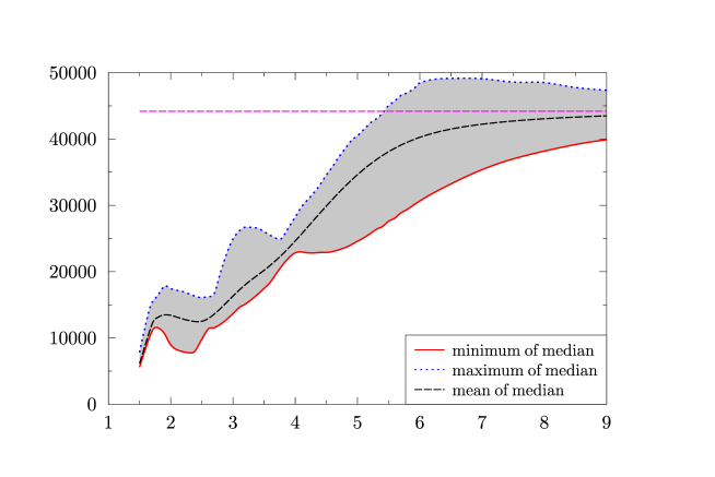
Figure 7: The width of the distribution of the position dependent median of $S(60^{\circ})$ is shown in dependence on the size $L$ of the regular Hantzsche-Wendt manifold. For each value of $L$, an ensemble of 50 000 CMB simulations is generated for each of the $51^{3}$ observer positions within the manifold, so that a distribution of $51^{3}$ median values of $S(60^{\circ})$ is obtained from which the mean, the minimum and the maximum is determined. The dashed horizontal line at $44182\mu\hbox{K}^{4}$ belongs to the median of the $\Lambda$CDM concordance model. Since there is no position dependence in this case, only one curve can be plotted.

The results are shown in figures 7 and 8. Figure 7 reveals the suppression of correlations compared to the $\Lambda$CDM concordance model, whose $S(60^{\circ})$ median is plotted as a horizontal line. For lengths below $L\simeq 4$, the large-scale correlations of the Hantzsche-Wendt space are at least a factor of two smaller than those of the $\Lambda$CDM model. For the minimum of the median, the suppression is remarkable even up to length scales of almost $L=5$ where the figure reveals a plateau. The diameter of the surface of last scattering is $D_{\hbox{\scriptsize sls}}=6.605$, so that the suppression is less pronounced for $L>D_{\hbox{\scriptsize sls}}$ as it is confirmed by figure 7. At $L=9$ the mean of the median of $S(60^{\circ})$ nearly agrees with the $\Lambda$CDM value. We showed in section 2 that the Hantzsche-Wendt space with $L>3$ will not be discovered by searches for matched back-to-back circle pairs. In the length interval $L=3$ to $L=6$ exists only one matched back-to-back circle pair with radius $\alpha>25^{\circ}$ and that only for very special observer positions $\vec{x}_{o}$. Therefore, there exists a range of sizes of the Hantzsche-Wendt space having a significant suppression of large-scale correlations without betraying themselves by back-to-back circle pairs for general observers.

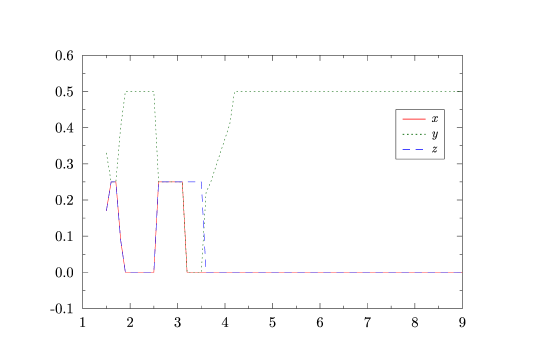
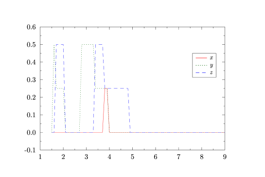
Figure 8: Panel (a) shows the positions $(x,y,z)$ of that observer for which the minimum of the median of $S(60^{\circ})$ is obtained as plotted in figure 7. Panel (b) reveals the corresponding positions for the maximum.

The positions $(x,y,z)$ of the observers for which the lowest and the highest values of the median of $S(60^{\circ})$ are found, can be read off from figure 8. Whereas panel (a) shows the positions for the smallest values of the median, panel (b) plots the positions for the maximum. One observes several switches for these positions. From $L=2.6$ to $L=3.1$, small medians occur at $(x,y,z)=\big{(}\frac{1}{4},\frac{1}{4},\frac{1}{4}\big{)}$. Around $L=3$ large medians belong to $(x,y,z)=\big{(}0,\frac{1}{2},0\big{)}$. It is interesting to note that exactly the position $\big{(}0,\frac{1}{2},0\big{)}$ corresponds to small medians for large spaces $L\geq 4.2$ which persists up to the largest investigated spaces with $L=9$. This position also leads to small medians between $L=2$ and $L=2.5$. Since the two positions $(x,y,z)=\big{(}\frac{1}{4},\frac{1}{4},\frac{1}{4}\big{)}$ and $\big{(}0,\frac{1}{2},0\big{)}$ are distinguished, we will investigate them in more detail below. The Dirichlet domain for these two cases is shown in figure 1, panels (b) and (d).

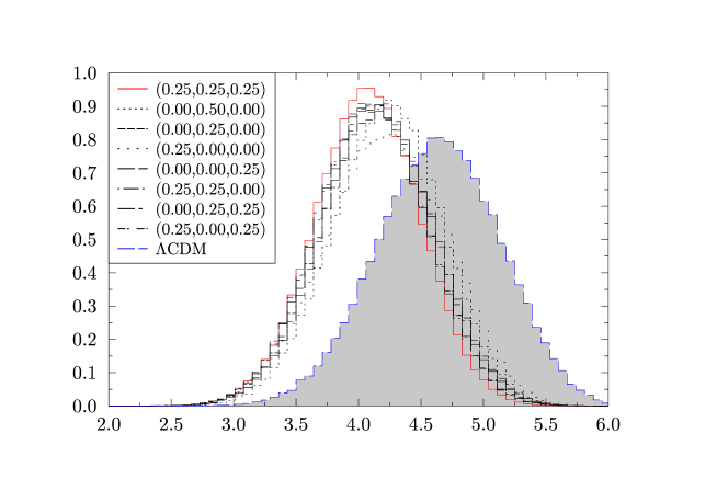
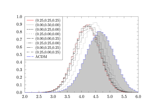
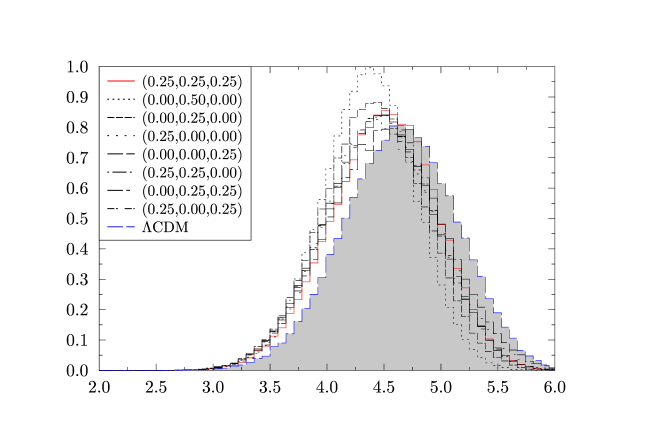
Figure 9: The distribution of $\log_{10}(S(60^{\circ}))$ is shown for three different topological lengths $L$ in panels (a) to (c). The histograms are computed from 100 000 simulations for various positions $(x,y,z)$ of the observer as stated in the legend. In addition, all panels show the corresponding distribution of the $\Lambda$CDM model.

Figure 7 shows the width of the distribution of the medians of $S(60^{\circ})$, and thus does not reveal the distribution of the medians for a fixed observer position $\vec{x}_{o}$. This information is provided by figure 9 which displays the distribution for several observer positions $\vec{x}_{o}$. Since the distributions are very asymmetrical having a pronounced tail towards large values, the histograms are plotted using a logarithmic scale. With such a scaling the distributions virtually look almost like Gaussians, but they are not, of course. For the three topological scales $L=2.7$, $L=3.1$, and $L=4.5$, the histograms belonging to 8 different positions are shown in comparison to the distribution of the $\Lambda$CDM model which is shaded in grey. All histograms are based on 100 000 simulations and reveal the position dependence of the distributions. The histograms show the degree of how much the distributions of the Hantzsche-Wendt space are shifted towards smaller medians of $S(60^{\circ})$ compared to the $\Lambda$CDM model. Note that due to the logarithmic scale, the difference between the Hantzsche-Wendt space and the infinite space is more pronounced than figure 9 suggests. The switch of the positions belonging to extreme medians described in connection with figure 8 can also be seen in figure 9. Panels (a) and (b), belonging to $L=2.7$ and $L=3.1$, respectively, show that the histogram belonging to $(x,y,z)=\big{(}\frac{1}{4},\frac{1}{4},\frac{1}{4}\big{)}$ is shifted towards small medians, while the histogram belonging to $\big{(}0,\frac{1}{2},0\big{)}$ is shifted towards the $\Lambda$CDM histogram. Panel (c), belonging to $L=4.5$, shows the reverse behaviour so that the distribution due to $\big{(}0,\frac{1}{2},0\big{)}$ has smaller medians as well as the most pronounced peak.

For $L=2.7$ there are 3 back-to-back circle pairs with a radius of $35^{\circ}$, and for the position $\vec{x}_{o}=\big{(}\frac{1}{4},0,0\big{)}$ lying on the axis of rotation of the first generator in (1) exists an additional one with $66^{\circ}$ (compare figure 4). The larger fundamental domain with $L=3.1$ does not possess back-to-back circle pairs with radii above $25^{\circ}$ except for the position $\vec{x}_{o}=\big{(}\frac{1}{4},0,0\big{)}$ where one occurs with radius $62^{\circ}$. The same applies for the space with $L=4.5$ except that for the special position the radius is reduced to $47^{\circ}$.

Since the CMB observations point to an exceedingly small value of $S(60^{\circ})$, the most important detail in the histograms lies in the left tail. The paper [36] discusses only the lack of large-angle correlations in the cut sky, but the values listed in their tables 1 and 2 are always below $1900\mu\hbox{K}^{4}$ for different combinations of CMB measurements and masks. Although these $S(60^{\circ})$ values refer to the cut sky, we nevertheless compute the corresponding values for our full-sky simulations. The cut-sky maps are discussed in the next section.

To calculate the likelihood that a given model has a correlation of $S(60^{\circ})$ below a given threshold $S_{\hbox{\scriptsize threshold}}$, a set of 100 000 CMB simulations is generated and the number of simulations having $S(60^{\circ})<S_{\hbox{\scriptsize threshold}}$ gives the probability $p(S_{\hbox{\scriptsize threshold}})$. For the $\Lambda$CDM model, one gets the probabilities $p(1000\mu\hbox{K}^{4})=0.044\%$, $p(1500\mu\hbox{K}^{4})=0.158\%$, and $p(2000\mu\hbox{K}^{4})=0.363\%$. For the Hantzsche-Wendt space we compute the probabilities for these thresholds for the observer position $\vec{x}_{o}$ belonging to the minimum of median of the $S(60^{\circ})$ distribution as shown in figure 8. Throughout the considered $L$ interval the Hantzsche-Wendt probabilities are higher than the corresponding ones of the $\Lambda$CDM model, as can be seen in figure 10. As expected for $L<D_{\hbox{\scriptsize sls}}$ the occurrences of small medians are much more likely for the Hantzsche-Wendt space than for the $\Lambda$CDM model. A pronounced peak probability occurs around $L\simeq 2.4$, see figure 10. Let us now turn to a comparison which takes a mask into account.

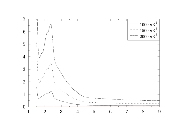
Figure 10: The probability given in percent $\%$ is plotted for obtaining a model with an value of $S(60^{\circ})$ below the threshold $1000\mu K^{4}$, $1500\mu K^{4}$, and $2000\mu K^{4}$, respectively. The probabilities are obtained from 100 000 simulations and the value is taken for that observer position for which the largest probability occurs. The straight horizontal lines give the corresponding probabilities of the $\Lambda$CDM model.

5.2 Analysis with WMAP mask kq75 9yr

In this section we analyse the reduction of large-scale correlations of the Hantzsche-Wendt topology in the presence of a mask. As pointed out in [36] the correlations on the cut sky are already unusually low, so that it is not compelling to delve into a full-sky reconstruction which will burden the analysis with unknown biases. Thus we will now focus on the cut-sky correlations which will be derived analogous to the observational data in order to provide an internally consistent comparison of the large-scale correlations.

The correlations of the Hantzsche-Wendt space are obtained according the following pipeline. At first the expansion coefficients of the temperature anisotropy (14) are computed using

$$a_{lm}\;=\;\sum_{\vec{k}}T_{l}(k)\,\sqrt{P(k)}\,\xi_{lm}^{\vec{k}}(\vec{x}_{o})\hskip 10.0pt,$$ (21)

where $\xi_{lm}^{\vec{k}}(\vec{x}_{o})$ is given by equation (13). Since the generators (1) single out the axes of the coordinate system, the CMB radiation is statistically anisotropic. Therefore, a random rotation is applied to the coefficients $a_{lm}$ which is done using the Wigner $D$ matrices $D_{m_{1}m_{2}}^{l}(\alpha,\beta,\gamma)$, where $\alpha,\beta,\gamma$ denote the Euler angles of the rotation. Choosing the rotation angles $\alpha,\beta,\gamma$ uniformly distributed over their definition interval, one gets simulated sky maps with a random orientation of the fundamental cell. In the next step the monopole and dipole is removed. Thereafter a full-sky map is generated and the kq75 9year mask of the WMAP team [37] is applied. From this cut-sky map the coefficients $\widetilde{a}_{lm}$ are computed which in turn lead to the pseudo-$C_{l}$

$$\widetilde{C}_{l}\;:=\;\frac{1}{2l+1}\sum_{m=-l}^{l}|\widetilde{a}_{lm}|^{2}\hskip 10.0pt.$$ (22)

This allows the computation of the pseudo-correlation function

$$\widetilde{C}(\vartheta)\;=\;\frac{1}{A(\vartheta)}\,\sum_{l=0}^{l_{\hbox{\scriptsize max}}}\,\frac{2l+1}{4\pi}\,\widetilde{C}_{l}\,P_{l}(\cos\vartheta)\hskip 10.0pt,$$ (23)

where

$$A(\vartheta)\;:=\;\sum_{l=0}^{l_{\hbox{\scriptsize max}}}\,\frac{2l+1}{4\pi}\,A_{l}\,P_{l}(\cos\vartheta)\hskip 10.0pt\hbox{ with }\hskip 10.0ptA_{l}:=\frac{1}{2l+1}\,\sum_{m=-l}^{l}|w_{lm}|^{2}$$ (24)

takes the correct normalisation into account. The spherical expansion coefficients of the mask are denoted by $w_{lm}$. Thereafter the final step is the calculation of $S(60^{\circ})$ from $\widetilde{C}(\vartheta)$.

We investigate the distribution of $S(60^{\circ})$ for the regular Hantzsche-Wendt space with $L=2.7$, $3.1$, and $4.5$. The two special points $(x,y,z)=\big{(}\frac{1}{4},\frac{1}{4},\frac{1}{4}\big{)}$ and $\big{(}0,\frac{1}{2},0\big{)}$ are selected for the observer positions. Then 200 different sets of Euler angles $\alpha,\beta,\gamma$ are randomly generated. For each of the 200 orientations of the fundamental cell, we compute the distributions of $S(60^{\circ})$ from 100 000 simulations as described above. The results are shown in figure 11 where an overlay of the 200 histograms is plotted for each case of $L$ and $\vec{x}_{o}$. In addition, the distribution for the $\Lambda$CDM model is displayed as the histogram shaded in grey. The application of the kq75 9yr mask modifies the $\Lambda$CDM histogram only slightly, as can be inferred from figure 11. Furthermore, the figure reveals the anisotropic behaviour of the cut-sky maps of the Hantzsche-Wendt space, since the histograms differ only in the orientation of the CMB maps determined by $\alpha,\beta,\gamma$. One sees that the histograms are significantly shifted towards smaller values of $S(60^{\circ})$ for $L=2.7$ and $L=3.1$ compared to the $\Lambda$CDM case.

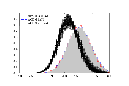
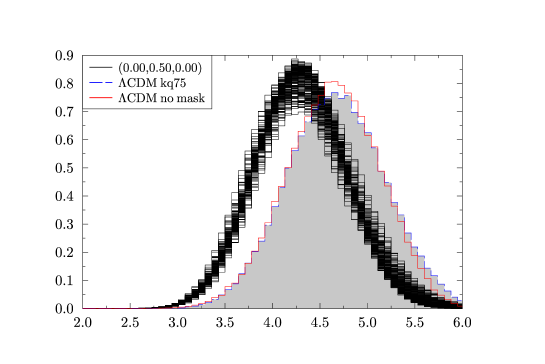
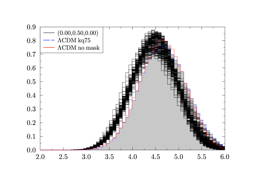
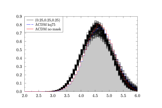
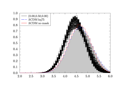
Figure 11: The distribution of $\log_{10}(S(60^{\circ}))$ is shown for three different topological lengths $L$ in panels (a) to (f). In contrast to figure 9, the distributions are computed for 200 random orientations of simulated sky maps relative to the kq75 mask. The histograms are based on 100 000 simulations for the observer position $(x,y,z)$ stated in the legend. In addition, all panels show the corresponding distribution of the $\Lambda$CDM model using the kq75 mask. To demonstrate the modest influence of the mask in the case of the $\Lambda$CDM simulations we also show its distribution without a mask.

Although the Hantzsche-Wendt topology possesses significantly smaller large-angle correlations than the $\Lambda$CDM model, the most interesting point lies in the tail of the distribution towards very small values of $S(60^{\circ})<2000\mu\hbox{K}^{4}$. To discuss that issue we compute the probabilities $p(S_{\hbox{\scriptsize threshold}})$ from the 200 histograms for the six cases shown in figure 11. The table 1 gives the result together with the probabilities belonging to the $\Lambda$CDM case with and without the application of a mask. One observes that, as expected, the probabilities $p(S_{\hbox{\scriptsize threshold}})$ are always enhanced with respect to the $\Lambda$CDM model.

model	position	$p(1000\mu\hbox{K}^{4})$	$p(1500\mu\hbox{K}^{4})$	$p(2000\mu\hbox{K}^{4})$
HW $L=2.7$	(0.25, 0.25, 0.25)	0.235%	0.891%	1.984%
HW $L=2.7$	(0.00, 0.50, 0.00)	0.174%	0.665%	1.492%
HW $L=3.1$	(0.25, 0.25, 0.25)	0.164%	0.642%	1.465%
HW $L=3.1$	(0.00, 0.50, 0.00)	0.079%	0.309%	0.719%
HW $L=4.5$	(0.25, 0.25, 0.25)	0.046%	0.196%	0.481%
HW $L=4.5$	(0.00, 0.50, 0.00)	0.049%	0.211%	0.525%
HW $L=9.0$	(0.00, 0.50, 0.00)	0.030%	0.131%	0.324%
3-torus $L=4.0$	independent	0.118%	0.511%	1.231%
$\Lambda$CDM kq75 9yr	independent	0.028%	0.103%	0.260%
$\Lambda$CDM no mask	independent	0.044%	0.158%	0.363%

Table 1: The probabilities $p(1000\mu\hbox{K}^{4})$, $p(1500\mu\hbox{K}^{4})$, and $p(2000\mu\hbox{K}^{4})$ are computed for CMB maps which are masked using a random orientation relative to the kq75 mask. The distributions of $S(60^{\circ})$ belonging to the first six models are shown in figure 11. Only the last row of the table refers to probabilities computed without applying a mask.

Since the 3-torus topology is well studied, it is interesting to compare it with the Hantzsche-Wendt topology. Because the volume of the regular Hantzsche-Wendt space is $2\,L^{3}$, i. e. twice that of the cubic 3-torus having a volume of $L^{3}$, the 3-torus length $L=4$ corresponds to the regular Hantzsche-Wendt space with $L=4/2^{1/3}\simeq 3.17$ by volume. So we compare the cubic 3-torus with $L=4$ with the Hantzsche-Wendt manifold with $L=3.1$ in the following. Although the 3-torus topology is homogeneous, its CMB radiation is not statistically isotropic. The same procedure that is applied to cut-sky simulations in the case of the Hantzsche-Wendt space is also applied for the 3-torus topology. Their CMB maps were rotated by randomly chosen Euler angles, and the kq75 mask is used. Figure 12 shows the histograms for the cubic 3-torus with $L=4$ analogous to figure 11 demonstrating the degree of anisotropy. The probabilities $p(S_{\hbox{\scriptsize threshold}})$ of this cubic 3-torus topology are also given in table 1. Since the 3-torus topology is homogeneous, it does not possess a position dependence, and a single row in the table suffices. Comparing the torus probabilities with the Hantzsche-Wendt space with $L=3.1$, one observes that they lie between the probabilities of the Hantzsche-Wendt observer positions belonging to the highest and the lowest probability, respectively. So one concludes that the suppression of large-scale correlations of the 3-torus is comparable to the Hantzsche-Wendt topology. However, the 3-torus has at that size several matched back-to-back circle pairs which contrasts to the Hantzsche-Wendt case as discussed in section 2.

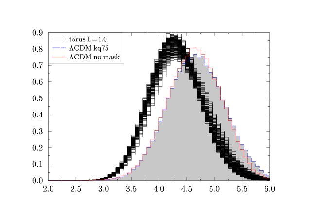
Figure 12: The distribution of $\log_{10}(S(60^{\circ}))$ is shown for the homogeneous cubic 3-torus topology with $L=4.0$. The kq75 9yr mask is applied to the torus simulations similar to figure 11.

6 Summary

The observed low amplitudes of large-angle temperature correlations $C(\vartheta)$ could be explained naturally by multiply connected spaces if their sizes fits well within the surface of last scattering from which the CMB radiation originates. Because of missing convincing hints for matched circle pairs in the CMB sky, the explanation for the suppression of correlations as a consequence of a non-trivial cosmic topology is currently somewhat disfavoured. We thus devote this paper to the Hantzsche-Wendt manifold which is a compact and orientable manifold and lives in the flat three-dimensional Euclidean space $\mathbb{E}^{3}$.

It is shown that the regular Hantzsche-Wendt space with lengths $L\gtrsim 3$ in units of the Hubble length $L_{\hbox{\scriptsize H}}$ possesses only for carefully selected observer positions a single matched back-to-back circle pair. For general observers there will be none. There are non-back-to-back circle pairs, but they are much harder to detect due to the enhanced background of spurious signals. It is shown that Hantzsche-Wendt spaces with $L\simeq 3$ possess large-angle correlations which are reduced around a factor of two or more in comparison to the $\Lambda$CDM concordance model. Furthermore, the amplitude of the correlations in the Hantzsche-Wendt topology is comparable to that of the 3-torus topology, if spaces of the same volume are considered. However, in contrast to the Hantzsche-Wendt space, the 3-torus has matched back-to-back circle pairs at that size.

So we conclude that a Hantzsche-Wendt space around $L\simeq 3$ is a very interesting topology for the spatial structure of our Universe which might escape the detection by searches after matched circle pairs and nevertheless has low large-angle temperature correlations.

References

References

- [1] M. Lachièze-Rey and J.-P. Luminet, Physics Report 254, 135 (1995).
- [2] J.-P. Luminet and B. F. Roukema, Topology of the Universe: Theory and Observation, in NATO ASIC Proc. 541: Theoretical and Observational Cosmology, p. 117, 1999, astro-ph/9901364.
- [3] J. Levin, Physics Report 365, 251 (2002).
- [4] M. J. Rebouças and G. I. Gomero, Braz. J. Phys. 34, 1358 (2004), astro-ph/0402324.
- [5] J.-P. Luminet, (2008), arXiv:0802.2236 [astro-ph].
- [6] B. Mota, M. J. Rebouças, and R. Tavakol, Phys. Rev. D 81, 103516 (2010), arXiv:1002.0834 [astro-ph.CO].
- [7] B. Mota, M. J. Rebouças, and R. Tavakol, Phys. Rev. D 84, 083507 (2011), arXiv:1108.2842 [astro-ph.CO].
- [8] H. Fujii and Y. Yoshii, Astron. & Astrophy. 529, A121 (2011), arXiv:1103.1466 [astro-ph.CO].
- [9] A. Riazuelo, J. Weeks, J.-P. Uzan, R. Lehoucq, and J.-P. Luminet, Phys. Rev. D 69, 103518 (2004), arXiv:astro-ph/0311314.
- [10] N. J. Cornish, D. N. Spergel, and G. D. Starkman, Class. Quantum Grav. 15, 2657 (1998), arXiv:astro-ph/9801212.
- [11] B. F. Roukema, Mon. Not. R. Astron. Soc. 312, 712 (2000), arXiv:astro-ph/9910272.
- [12] B. F. Roukema, Class. Quantum Grav. 17, 3951 (2000), arXiv:astro-ph/0007140.
- [13] N. J. Cornish, D. N. Spergel, G. D. Starkman, and E. Komatsu, Phys. Rev. Lett. 92, 201302 (2004), arXiv:astro-ph/0310233.
- [14] B. F. Roukema, B. Lew, M. Cechowska, A. Marecki, and S. Bajtlik, Astron. & Astrophy. 423, 821 (2004), arXiv:astro-ph/0402608.
- [15] R. Aurich, S. Lustig, and F. Steiner, Mon. Not. R. Astron. Soc. 369, 240 (2006), arXiv:astro-ph/0510847.
- [16] H. Then, Mon. Not. R. Astron. Soc. 373, 139 (2006), arXiv:astro-ph/0511726.
- [17] J. S. Key, N. J. Cornish, D. N. Spergel, and G. D. Starkman, Phys. Rev. D 75, 084034 (2007), arXiv:astro-ph/0604616.
- [18] R. Aurich, H. S. Janzer, S. Lustig, and F. Steiner, Class. Quantum Grav. 25, 125006 (2008), arXiv:0708.1420 [astro-ph].
- [19] P. Bielewicz and A. J. Banday, Mon. Not. R. Astron. Soc. 412, 2104 (2011), arXiv:1012.3549 [astro-ph.CO].
- [20] P. M. Vaudrevange, G. D. Starkman, N. J. Cornish, and D. N. Spergel, Phys. Rev. D 86, 083526 (2012), arXiv:1206.2939 [astro-ph.CO].
- [21] B. Rathaus, A. Ben-David, and N. Itzhaki, Journal of Cosmology and Astroparticle Physics 10, 45 (2013), arXiv:1302.7161 [astro-ph.CO].
- [22] R. Aurich and S. Lustig, Mon. Not. R. Astron. Soc. 433, 2517 (2013), arXiv:1303.4226 [astro-ph.CO].
- [23] Planck Collaboration et al., (2013), arXiv:1303.5086 [astro-ph.CO].
- [24] W. Hantzsche and H. Wendt, Math. Annalen 110, 593 (1935).
- [25] E. Scannapieco, J. Levin, and J. Silk, Mon. Not. R. Astron. Soc. 303, 797 (1999), arXiv:astro-ph/9811226.
- [26] J. Levin, E. Scannapieco, and J. Silk, Phys. Rev. D 58, 103516 (1998), arXiv:astro-ph/9802021.
- [27] N. Jarosik et al., Astrophys. J. Supp. 192, 14 (2011), arXiv:1001.4744 [astro-ph.CO].
- [28] O. Fabre, S. Prunet, and J.-P. Uzan, (2013), arXiv:1311.3509 [astro-ph.CO].
- [29] Planck Collaboration et al., (2013), arXiv:1303.5076 [astro-ph.CO].
- [30] A. Riazuelo, J. Uzan, R. Lehoucq, and J. Weeks, Phys. Rev. D 69, 103514 (2004), astro-ph/0212223.
- [31] C. Ma and E. Bertschinger, Astrophys. J. 455, 7 (1995).
- [32] W. Hu, Wandering in the Background: A CMB Explorer, PhD thesis, University of California at Berkeley, 1995, arXiv:astro-ph/9508126.
- [33] J. R. Bond, D. Pogosyan, and T. Souradeep, Class. Quantum Grav. 15, 2671 (1998).
- [34] K. T. Inoue and N. Sugiyama, Phys. Rev. D 67, 043003 (2003), astro-ph/0205394.
- [35] G. Aslanyan, A. V. Manohar, and A. P. S. Yadav, Journal of Cosmology and Astroparticle Physics 8, 9 (2013), arXiv:1304.1811 [astro-ph.CO].
- [36] C. J. Copi, D. Huterer, D. J. Schwarz, and G. D. Starkman, (2013), arXiv:1310.3831 [astro-ph.CO].
- [37] C. L. Bennett et al., Astrophys. J. Supp. 208, 20 (2013), arXiv:1212.5225 [astro-ph.CO].
- [38] G. Hinshaw et al., Astrophys. J. Lett. 464, L25 (1996).
- [39] C. J. Copi, D. Huterer, D. J. Schwarz, and G. D. Starkman, Mon. Not. R. Astron. Soc. 399, 295 (2009), arXiv:0808.3767 [astro-ph].
- [40] D. N. Spergel et al., Astrophys. J. Supp. 148, 175 (2003), arXiv:astro-ph/0302209.