The expansion rate of the intermediate universe in light of Planck
Abstract
We use cosmology-independent measurements of the expansion history in the redshift range and compare them with the Cosmic Microwave Background-derived expansion history predictions. The motivation is to investigate if the tension between the local (cosmology independent) Hubble constant value and the Planck-derived is also present at other redshifts. We conclude that there is no tension between Planck and cosmology independent-measurements of the Hubble parameter at for the CDM model (odds of tension are only 1:15, statistically not significant). Considering extensions of the CDM model does not improve these odds (actually makes them worse), thus favouring the simpler model over its extensions. On the other hand the data are also not in tension with the local measurements but the combination of all three data-sets shows a highly significant tension (odds ). Thus the new data deepen the mystery of the mismatch between Planck and local measurements, and cannot univocally determine wether it is an effect localised at a particular redshift. Having said this, we find that assuming the NGC4258 maser distance as the correct anchor for , brings the odds to comfortable values.
Further, using only the expansion history measurements we constrain, within the CDM model, and without relying on any CMB prior. We also address the question of how smooth the expansion history of the universe is given the cosmology independent data and conclude that there is no evidence for deviations from smoothness on the expansion history, neither variations with time in the value of the equation of state of dark energy.
keywords:
Cosmology, Hubble parameter, Cosmic Microwave Background, Bayesian methods1 Introduction
The recent release of the determination of cosmological parameters from the Planck [1, 2] Cosmic Microwave Background (CMB) observations, has shown that for a CDM model, the extrapolated value at of the Hubble parameter, , is in tension with the one measured locally via astronomical observations of the local distance scale [3, 4]. This could be due to unaccounted systematics in the data in either (or both) experiment, or to a failure of the adopted cosmological model to describe nature.
In a previous paper [3] we discussed the importance of local () measurements in order to assess the consistency of the currently favoured cosmology model: CDM. Because the CMB mostly probes the universe at , any cosmological parameter defined at any other redshift is necessarily model-dependent. Therefore, if cosmological parameters can be measured directly, precisely and robustly at other redshifts than , the comparison with the same quantities derived from the CMB using the standard CDM model can serve as a test of the model itself.
In Ref. [4] we concluded that local measurements of the expansion rate () and of the age of the Universe were in tension (odds 1:53) with the Planck-derived parameters from the CMB within the CDM model. The tension was driven by and not by the age. With only the data-sets considered there, it was however not possible to determine wether this tension is a signature of systematics in either measurement or new physics: independent data are needed to make further progress.
One way to further investigate this is to “fill the gap” by focusing on but still . This can be done by using the recent measurements of between redshift from the cosmic chronometers project [5, 6, 7, 8, 9]. This adds cosmology-independent measurements of the expansion rate back to when the Universe was only of its current age ( to the distance of last-scattering), thus significantly increasing the volume surveyed in the Universe to test the CMB-derived cosmology model. The cosmic chronometer method is the only method that provides cosmology-independent, direct measurements of the expansion history of the universe. In fact, Supernovae data measure the luminosity distance-redshift relation, which is related to an integral of . However the necessary marginalisation over the (unknown) intrinsic magnitude of the standard candles is effectively equivalent to a marginalisation over an overall amplitude i.e., over . Baryon acoustic oscillations must rely on the CMB measurement of a standard ruler (the sound horizon at radiation drag) to extract information from radial clustering; angular clustering yields a combination of the angular diameter distance and the sound horizon at radiation drag and angle averaged clustering yields a combination of angular diameter distance, and sound horizon. While the CMB determination of the sound horizon is robust e.g., Ref. [10] it is still somewhat model-dependent (e.g., [11, 12, 13]). Following Ref. [9] we concentrate on the redshift range where the dependence on the assumed stellar model is small.
In this paper we explore whether the expansion history at intermediate redshifts shows any signature of possible deviations from the CMB-inferred one. The paper is organised as follows: we first investigate (§2), in a mostly parameter-independent way via Gaussian Processes (GP), if the data show any sign of the expansion not being smooth: we find none. We also find no evidence for variations of the dark energy equation of state parameter (§3). We then explore the constraints on the parameters of several cosmological models (the standard CDM and its popular extensions) using only data and no CMB prior (§4). Finally we compute the tension between the data and the Planck-derived expansion history for different cosmological models (§5). We conclude in §6.
2 Is the expansion history “smooth”?
Here and in what follows we use the cosmology-independent expansion history measurements from Refs. [6, 7, 9]. Ref. [9] showed that at the dependence on the assumed stellar population model becomes important. A full treatment that marginalises over the model uncertainty will be presented elsewhere, here we only consider . In addition we increase slightly (20%) the error bars of the point at to encompass the stellar model uncertainty.
We start by investigating if there are any signatures of deviation from smoothness using Gaussian Processes (GP) [14, 15], which is a non-parameric Bayesian inference formalism. Ref. [17] have been the first ones to recently use GP on the same dataset to extrapolate the value of the the Hubble parameter at assuming smoothness of the expansion history. Here we use GP with a different purpose: to determine, in the least parametric way, if the data show any deviation from smoothness as a function of redshift.
We will not enter into a detailed description of GPs here but instead refer the interested reader to the literature (see e.g., [14, 15] for standard references in the field). GP is a stochastic process that considers independent and identically distributed Gaussian measurement errors, the relations or correlations between measurements are defined via a covariance matrix. Using standard Bayesian methodology, the estimation of at any value of is determined by a probability distribution (posterior predictive). This results into a fully probabilistic estimation of the expansion history given the measurements. In our application the different determinations are uncorrelated, therefore the off-diagonal terms of the covariance matrix determine the smoothness of the fitting function. In this approach, the only choice we have to make is the form of the off diagonal terms of the covariance matrix. We have experimented with various choices of the covariance matrix with similar results, but we report here the outcome of employing the most commonly used covariance matrix, the radial exponential:
| (1) |
where and are two different z values (i.e., ) and , are the latent parameters or hyper-parameters which are determined using data themselves. Intuitively, controls the correlation length and therefore the “smoothness” and controls the importance of the off-diagonal terms compared to the diagonal ones. The bigger the is, the smoother the predictive function would look. Similarly, the higher the is the lower the signal-to-noise ratio is. The values of and can be obtained using maximum likelihood estimation. Since we are dealing with hyper-parameters and not parameters, we maximise the marginal likelihood (over functions) and not the likelihood directly. Note that this approach is the same as the hierarchical Bayesian one [16]. To do so we calculate the partial derivative of the marginal likelihood with respect to the hyper-parameters and optimise the hyper-parameters using gradient based search [14].
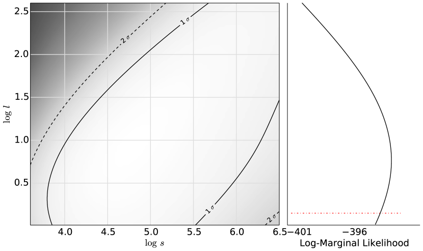
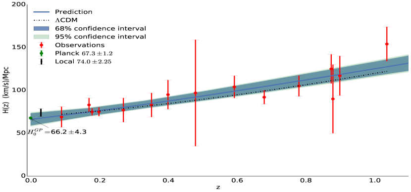
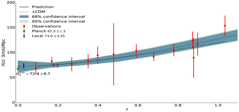
Fig.1 shows the marginalized likelihood given the data as a function of the two hyperparameters, and . The right panel shows the marginalized full likelihood (left panel) over . The dotted red line indicates the 5% confidence of the hyperparameter. This lower bound gives us the least smooth predictive posterior shown in Fig. 2.
The top panel of Fig. 2 shows the 68% and 95% confidence bound of the predicted posterior using the GP with the radial exponential covariance and the best estimate for the hyper-parameters, as described above. The bottom panel shows the same prediction but using hyper-parameters that produce the 5% least smooth features.
These regions are fully compatible with the Planck CMB derived expansion rate (dot-dashed line). But more interestingly is the fact that there is no signature for deviations from smoothness even when we considered the least likely value of that creates the least smooth curve. Any sharp or asymmetric variation of the equation of state parameter, , that results in a non-smooth expansion history, does not seem to be present at the accuracy of the data.
Another interesting feature is the value of the extrapolation at (as already pointed out and studied by Ref. [17]). While the error at is larger than the one from Planck 111The Planck determination reported here assumes a flat CDM model., it is fully compatible with it. It however points to the central value of the locally determined being slightly high. Here we use the Ref. [3] “world average” value for obtained from the [18] and [19] determinations.
3 Does w vary with time?
In this section, we examine possible variations of the dark energy equation of state parameter as a function of . We use the CDM model as the true model and we simply ask if for different domains of the best estimates of are statistically different or similar222We use weakly informative priors: uniform prior on between 0 and 1, Gaussian prior on centred around Km s-1Mpc-1 with a width of 10 Km s-1Mpc-1 and uniform prior on between -2 and 0.. We first estimate all three parameters for the whole dataset and then we divide the data into subsets and compare the posteriors of looking for significant statistical differences. For easy reference, in the appendix we report useful formulae for the expression of as a function of cosmological parameters.
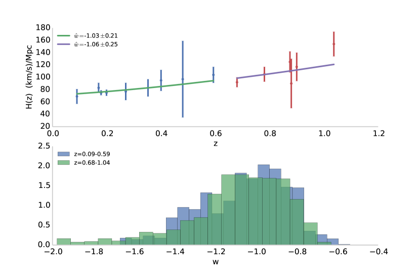
We perform multiple tests by dividing the data into different subsets and repeat the experiment many times. None of these tests produce any significant evidence that varies above the noise of the measurement given the CDM model. In order to enhance the power of our test, we fixed the values of and to the values estimated from the whole data set and repeat the test looking for statistically different values of , an indication of a varying . This is shown in Fig. 3. In this particular test the data were divided into two sub-sets and we find the marginalised posteriors for for both sub-sets. On the top panel we show the results of the fit using Bayesian linear regression, where on the bottom we compared the marginalized posteriors. All test we performed show similar results. We conclude that given the measurement error is invariant in time.
4 What does the expansion history tell us about the cosmological model?
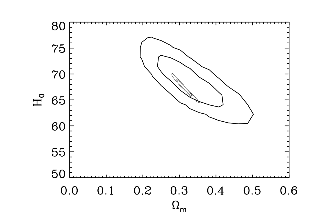
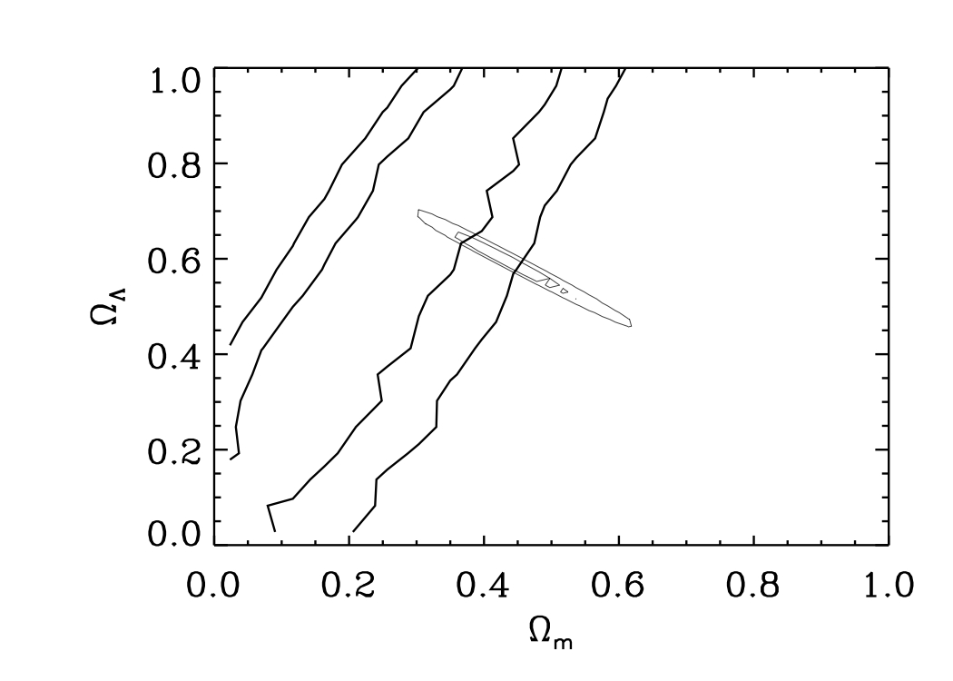
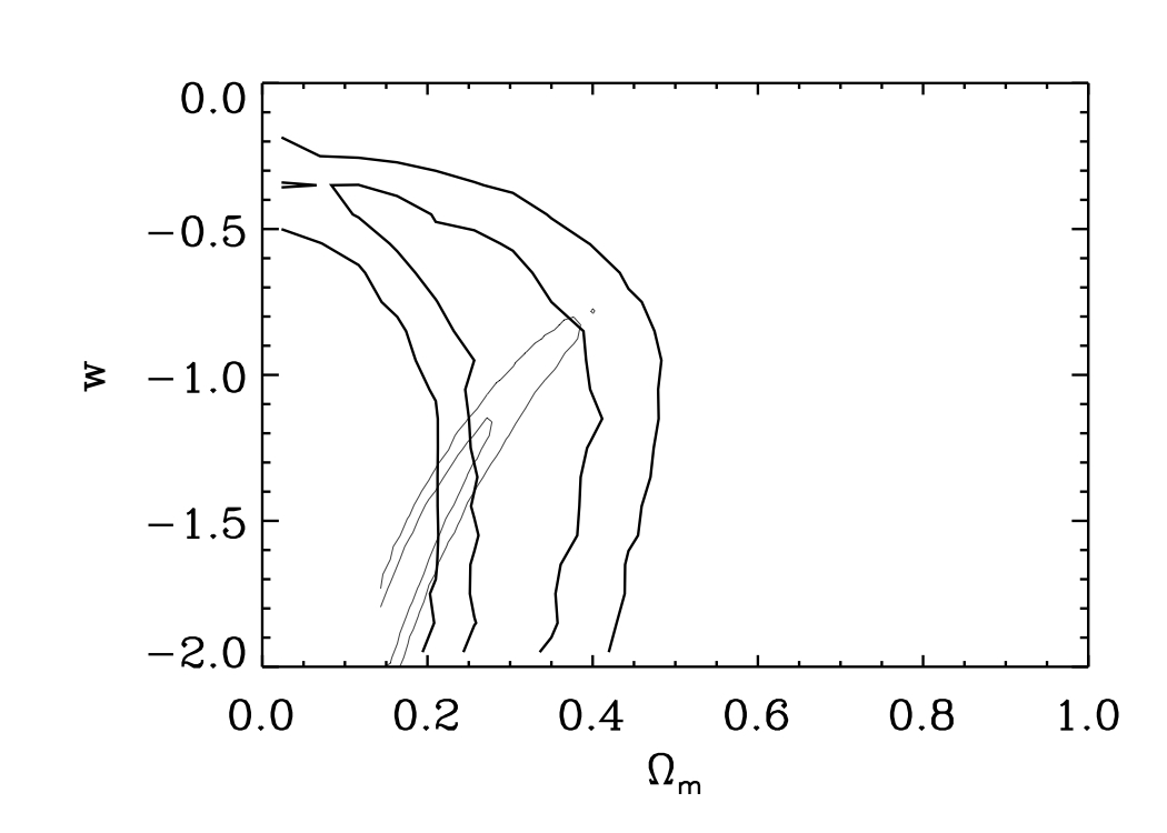
It is interesting to investigate what constraints on cosmology (cosmological models and parameters) one can impose by using only the cosmic chronometers data. This is shown in table 1 and Fig. 4. The models we consider are: the standard CDM, CDM where the (constant) parameter describing the equation of state of dark energy can differ from , oCDM where we allow the curvature to be non-zero and finally CDM, where the Universe is spatially flat but the equation of state of dark energy can change as a function of time. The constraints are qualitatively similar (and in agreement with) to the ones obtained from Supernovae type 1 A data, perhaps not surprisingly given that cosmic chronometers and supernovae are probes of the expansion history. As illustrated in Fig. 4 the constraints and degeneracy direction in parameter space, for models that are generalisations of the CDM are complementary to the ones obtained from the CMB.
| model | ||||||
|---|---|---|---|---|---|---|
| CDM | 0 | |||||
| wCDM | (95%) | 0 | (95%) | |||
| oCDM | (95 %) | – | – | – | ||
| (95 %) | – | – | – | – | – |
When considering marginalised constraints on single parameters, table 1 shows that the CDM model is fairly well constrained for the two parameters that affect the expansion history ( and the density parameter ). Once the CDM is extended, the cosmic chronometers data by themselves are not very constraining, being able to provide only upper(lower) limits on the parameters of the cosmology model. It is worth noting that for the most general extension of the CDM model (CDM) has to be larger than km s-1 Mpc-1.
5 Comparing with the universe at
In Ref. [4] we introduced a new statistical tool to determine the odds of two distributions being in tension and thus decide if one could combine the two distributions to further restrict the parameter space of the model. We briefly review here our main argument for completeness and to clarify notation.
Imagine we have performed two experiments: and for each experiment we produce a posterior where represents the parameters of the model and represents the data from experiments respectively. Let us also assume that for producing both posteriors we have used the same, uniform priors over the same “support”, x, i.e., , or and therefore . Let be the (null) hypothesis that both experiments measure the same quantity, the models are correct and there are no unaccountable errors. In this case, the two experiments will produce two posteriors, which, although can have different (co)variances, and different distributions, have means that are in agreement. The alternative hypothesis, is when the two experiments, for some unknown reason, do not agree, either because of systematic errors or because they are effectively measuring different things or the model (parameterization) is incorrect. In this case, the two experiments will produce two posteriors with two different means and different variances. To distinguish the two hypothesis we use the Bayes factor, imagine that we can perform a translation (shift) of (one or both of) the distributions in and let us define the shifted distribution. This translation changes the location of the maximum but does not change the shape or the width of the distribution. If the maxima of the two distributions coincide then
| (2) |
This can be considered our “straw man” null hypothesis (). As the distance between the maxima increases (but the shape of the distributions remains the same),
| (3) |
and eventually as the two distributions diverge. Clearly the Evidence ratio for the (null) hypothesis is , as the normalization factors cancel out, and the Evidence ratio for the alternative is its reciprocal. We therefore introduce:
| (4) |
which denotes the degree of tension that can be interpreted in the widely used (slightly modified, [21]) Jeffrey’s [20] scale. indicates the odds: are the chances for the null hypothesis. In other words, a large tension means that the null hypothesis ( = ) is unlikely.
Continuing on with the logic outlined above, let us consider that experiment A gives us the prior and experiment B gives us the data. is the evidence ratio between the integrated posterior in two cases. On the numerator: the prior from experiment A has a maximum that coincides with the maximum likelihood from experiment B; on the denominator: the prior from experiment A has a maximum that happened to be where it is.333Note that here one could loosely exchange “likelihood” with “posterior” for experiment B since we assume uniform priors for experiments A and B that are either 1 or 0 over the same “support” and therefore one can absorb the prior for experiment B into the A prior. Note that since the evidence is translation-invariant it does not matter which data set is considered as prior and which one as “data”: the result is symmetric.
This argument can be extended to as many measurements as we want: the relevant integral just becomes higher-dimensional. For example let us consider the 15 measurements in light of a Planck CMB prior for .
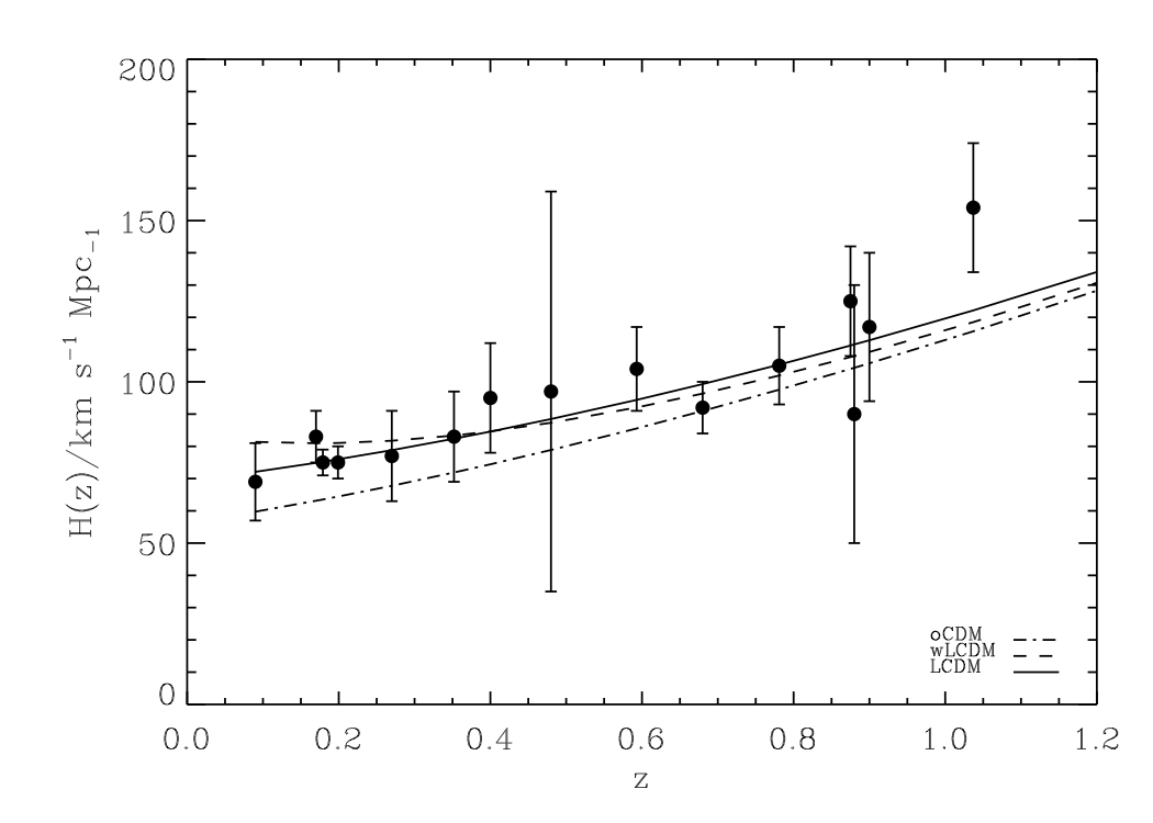
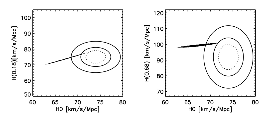
Table 2 shows the tension and odds for three different cosmology models while Fig. 5 shows the corresponding expansion history.
The first result to note is that the odds of the expansion history data and the Planck CMB CDM model derived parameters being in tension are very low: just 1:15, which is above 1 but below 2 ; we conclude that for the redshift range there is no evidence for tension between “local” data and CMB model derived expansion parameters. We also note that extensions to the CDM model are in tension with the “local” data, thus disfavouring extensions to the minimal CDM model.
| model | odds | |
|---|---|---|
| CDM | 2.73 | 1:15 |
| CDM | 3.27 | 1:26 |
| oCDM | 4.93 | 1:138 |
Ref. [23] excludes the 217 GHz channel from the analysis with the motivation that it has been shown to fail a number of null tests and therefore could be affected by some systematics. They also independently re-do the cleaning and analysis. As a result some of the parameters show some shifts, most notably (down by ) and (up by ): ; . We do not have access to their full posterior therefore we shift the Planck posteriors to be centred to these values and we refer to this as Planck “revisited”. This underestimates the final error-bars by some 20-30% but it is a conservative estimate of the agreement of the new analysis with lower redshift measurements. Ref. [22] studies the dependence of the measurement on the choice of distance scale anchor and on the procedure for outliers rejection. LMC and MW cepheids distance anchor yield values of in agreement with each other but NGC 4258 maser distance gives lower values.
Using all distance anchors he obtains km s-1Mpc-1 while using the maser distance yields km s-1Mpc-1. The combination LMC + MW yields a value very close to the “world average” ( in this table) used above (we do not consider this combination below as results are virtually unchanged). In table 3 we report the results of the various combinations; the tension between CMB and cosmic chronometers remains virtually unchanged between the original Planck and the revisited Planck constraints.
| data combination | Planck orig. | Planck Revisited | ||
|---|---|---|---|---|
| odds | odds | |||
| Planck+ | 2.73 | 1:15 | 2.71 | 1:14 |
| Planck + | 3.55 | 1:35 | 2.85 | 1:17 |
| Planck + | 0.44 | 1:1.6 | 0.27 | 1:1.3 |
| Planck + | 1.77 | 1:6 | 1.33 | 1:3.7 |
| Planck++ | 6.17 | 1:473 | 5.5 | 1:245 |
| Planck++ | 3.1 | 1:22 | 3.0 | 1:20 |
| Planck++ | 4.4 | 1:81 | 4.0 | 1:55 |
Clearly both re-analyses lower the tension. If only Planck and the local measurements are considered either reanalysis brings the tension to comfortable values, but if all measurements are considered (i.e. we consider a 16 dimensional tension) both re-analyses are needed and only the maser distance brings the odds to comfortable values. Note that + are consistent with each other (odds 1:2.4, ). What we see here is the power of combining many different determinations and therefore evaluating the tension in high-dimensions. When degeneracies are present (as for example in the case of the Planck extrapolated values of ) single determinations might be in agreement but the multi-dimensional distribution might be less so; this is illustrated in Fig. 6.
6 Discussion and Conclusions
Using the cosmology independent expansion history data () from the compilation of Ref. [9] we have explored if the intermediate redshift universe is in tension with the Planck CDM derived one. To do so we have generalised the two-dimensional tension introduced in Ref. [4] to an arbitrary number of dimensions. The inclusion of new data adds cosmology-independent measurements of the expansion rate back to when the Universe was only of its current age ( to the distance of last-scattering), thus significantly increasing the volume surveyed to test the CMB-derived cosmology model. We find no tension (odds only 1:15) between Planck and . This is in contrast with the local universe () which is in significant tension [4] (1:57) with Planck. However and are not in tension within a CDM model: the central value for the Hubble constant obtained from happens to be very near the Planck-CMB inferred one, but the error-bars are larger. When considering the three datasets–Planck, and – the tension becomes highly significant (odds become uncomfortably low ). Thus the addition of deepens the mystery of the mis-match between Planck and local measurements, and cannot univocally determine wether it is an effect localised at or or if it shows as a smooth change of the measured value of as a function of the redshift of the measurement.
Both the Planck and the local measurements have been independently re-visited and re-analysed. Either re-analysis brings the tension between Planck and local measurements to comfortable level. On the other hand, when the three datasets are considered the Planck re-analysis has very little effect, and only assuming the NGC4258 maser distance as the correct anchor for brings the odds to comfortable values. However at present there are no compelling reasons to discard the other anchors [18, 22].
The highly significant tension for the combined data set within the CDM model however warrants further investigation: if we were to interpret the number in terms of Gaussian standard deviations it would correspond to 4.9 . Of course at this level it is very important to know extremely well the tails of the distributions, here we have assumed that all errors on measurements of and are Gaussian and this might not be exact. The intermediate redshift measurements from the cosmic chronometers project, seems not to be explicitly in tension either with the nor with the CMB. Elsewhere (Cuesta et al. 2014 in prep.) we will consider other probes of the expansion history that cover a similar redshift range: baryon acoustic oscillations and supernovae. Moreover significant improvements in the measurements is forthcoming (Moresco et al. 2014 in prep.), the significantly smaller error-bars might be able to localise or to point to a possible reason for the tension.
We have also explored how smooth the expansion history data are. This is motivated by the fact that we wanted to investigate if with cosmology independent expansion history data we could see departures from a cosmological constant prediction. Using gaussian processes we concluded that the data are smooth with no sign of sharp deviations from a constant equation of state of dark energy over the redshift range .
Acknowledgements
LV is supported by FP7- IDEAS Phys.LSS 240117. LV and RJ are supported by MICINN grant FPA2011-29678.
Appendix: Useful formulas
For completeness we report here the expressions for for a homogeneous and isotropic FRW Universe.
For a flat universe, generic equation of state parameter for dark energy
| (5) |
for a non-flat Universe, equation of state parameter for dark energy given by the parameterization:
| (6) |
of course for a flat CDM model we have:
| (7) |
References
- [1] P. A. R. Ade et al. [Planck collaboration], arXiv:1303.5062
- [2] P. A. R. Ade et al.[Planck collaboration], arXiv:1303.5076
- [3] L. Verde, R. Jimenez and S. Feeney, Phys. Dark Univ. 2 (2013) 65 [arXiv:1303.5341 [astro-ph.CO]].
- [4] L. Verde, P. Protopapas and R. Jimenez, Phys. Dark Univ. 2 (2013) 166 [arXiv:1306.6766 [astro-ph.CO]].
- [5] R. Jimenez, A. Loeb, Astrophys. J. 573 (2002) 37-42. [astro-ph/0106145].
- [6] J. Simon, L. Verde, R. Jimenez, Phys. Rev. D71 (2005) 123001. [astro-ph/0412269].
- [7] D. Stern, R. Jimenez, L. Verde, M. Kamionkowski, S. A. Stanford, JCAP 1002 (2010) 008. [arXiv:0907.3149 [astro-ph.CO]].
- [8] M. Moresco, R. Jimenez, A. Cimatti, L. Pozzetti, JCAP 1103 (2011) 045. [arXiv:1010.0831 [astro-ph.CO]].
- [9] M. Moresco, A. Cimatti, R. Jimenez, L. Pozzetti, G. Zamorani, M. Bolzonella, J. Dunlop and F. Lamareille et al., JCAP 1208 (2012) 006 [arXiv:1201.3609 [astro-ph.CO]].
- [10] Eisenstein D. J., and White, M. J., Phys. Rev. D 70 (2004) 103523
- [11] Linder, E. V. and Robbers, G., JCAP 0806, 004 (2008)
- [12] de Bernardis, F., Bean, R., Galli, S., et al. 2009, PRD, 79, 043503
- [13] Mangilli, A., Verde, L., & Beltran, M. 2010, JCAP, 10, 9
- [14] C. Rasmussen and C. K. I. William, The MIT Press, 2006. ISBN 0-262-18253-X.
- [15] C. M. Bishop Pattern Recognition and Machine Learning. Springer, 2006.
- MacKay [1992] MacKay, D. J. C. 1992, Neural Computation 4 (3): 415 447
- [17] V. C. Busti, C. Clarkson and M. Seikel, arXiv:1402.5429 [astro-ph.CO].
- [18] Riess, A. G., Macri, L., Casertano, S., et al. 2011, ApJ, 730, 119
- [19] Freedman, W. L., et al. 2012, ApJ, 758, 24
- [20] Jeffreys, H., 1973. Scientific Inference. Cambridge University Press.
- [21] Kass, R.E. and Raftery, A. E., 1995, JASA 90, 430, 773-795.
- [22] Efstathiou, G. 2013. ArXiv e-prints arXiv:1311.3461.
- [23] Spergel, D., Flauger, R., Hlozek, R. 2013. ArXiv e-prints arXiv:1312.3313.