Constraint-based Causal Discovery from Multiple Interventions over Overlapping Variable Sets

\nameSofia Triantafillou \emailstriant@ics.forth.gr
\nameIoannis Tsamardinos \emailtsamard@ics.forth.gr
\addrInstitute of Computer Science
Foundation for Research and Technology - Hellas (FORTH)
N. Plastira 100 Vassilika Vouton
GR-700 13 Heraklion, Crete, Greece
Also in Department of Computer Science, University of Crete.
Abstract

Scientific practice typically involves repeatedly studying a system, each time trying to unravel a different perspective. In each study, the scientist may take measurements under different experimental conditions (interventions, manipulations, perturbations) and measure different sets of quantities (variables). The result is a collection of heterogeneous data sets coming from different data distributions. In this work, we present algorithm COmbINE, which accepts a collection of data sets over overlapping variable sets under different experimental conditions; COmbINE  then outputs a summary of all causal models indicating the invariant and variant structural characteristics of all models that simultaneously fit all of the input data sets. COmbINE  converts estimated dependencies and independencies in the data into path constraints on the data-generating causal model and encodes them as a SAT instance. The algorithm is sound and complete in the sample limit. To account for conflicting constraints arising from statistical errors, we introduce a general method for sorting constraints in order of confidence, computed as a function of their corresponding p-values. In our empirical evaluation, COmbINE  outperforms in terms of efficiency the only pre-existing similar algorithm; the latter additionally admits feedback cycles, but does not admit conflicting constraints which hinders the applicability on real data. As a proof-of-concept, COmbINE  is employed to co-analyze 4 real, mass-cytometry data sets measuring phosphorylated protein concentrations of overlapping protein sets under 3 different interventions.

1 Introduction

Causal discovery is an abiding goal in almost every scientific field. In order to discover the causal mechanisms of a system, scientists typically have to perform a series of experiments (interchangeably: manipulations, interventions, or perturbations). Each experiment adds to the existing knowledge of the system and sheds light to the sought-after mechanism from a different perspective. In addition, each measurement may include a different set of quantities (variables), when for example the technology used allows only a limited number of measured quantities.

However, for the most part, machine learning and statistical methods focus on analyzing a single data set. They are unable to make joint inferences from the complete collection of available heterogeneous data sets, since each one is following a different data distribution (albeit stemming from the same system under study). Thus, data sets are often analyzed in isolation and independently of each other; the resulting knowledge is typically synthesized ad hoc in the researcher’s mind.

The proposed work tries to automate the above inferences. We propose a general, constraint-based algorithm named COmbINE  for learning causal structure characteristics from the integrative analysis of collections of data sets. The data sets can be heterogeneous in the following manners: they may be measuring different overlapping sets of variables 𝐎isubscript𝐎𝑖{\bf O}_{i} under different hard manipulations on a set of observed variables 𝐈isubscript𝐈𝑖{\bf I}_{i}. A hard manipulation on a variable I𝐼I, corresponds to a Randomized Controlled Trial (Fisher, 1922) where the experimentation procedure completely eliminates any other causal effect on I𝐼I (e.g., randomizing mice to two groups having two different diets; the effect of all other factors on the diet is completely eliminated).

What connects together the available data sets and allows their co-analysis is the assumption that there exists a single underlying causal mechanism that generates the data, even though it is measured with a different experimental setting each time. A causal model is plausible as an explanation if it simultaneously fits all data-sets when the effect of manipulations and selection of measured variables is taken into consideration.

COmbINE  searches for the set of causal models that simultaneously fits all available data-sets in the sense given above. The algorithm outputs a summary network that includes all the variant and invariant pairwise causal characteristics of the set of fitting models. For example, it indicates the causal relations upon which all fitting models agree, as well as the ones for which conflicting explanations are plausible. As our formalism of choice for causal modeling, we employ Semi-Markov Causal Models (SMCMs). SMCMs (Tian and Pearl, 2003) are extensions of Causal Bayesian Networks (CBNs) that can account for latent confounding variables, but do not admit feedback cycles. Internally, the algorithm also makes heavy use of the theory and learning algorithm for Maximal Ancestral Graphs (MAGs) (Richardson and Spirtes, 2002).

The algorithm builds upon the ideas in Triantafillou et al. (2010) to convert the observed statistical dependencies and independencies in the data to path constraints on the plausible data generating structures. The constraints are encoded as a SAT instance and solved with modern SAT engines, exploiting the efficiency of state-of-the-art solvers. However, due to statistical errors in the determination of dependencies and independencies, conflicting constraints may arise. In this case, the SAT instance is unsolvable and no useful information can be inferred. COmbINE  includes a technique for sorting constraints according to confidence: The constraints are added to the SAT instance in increasing order of confidence, and the ones that conflict with the set of higher-ranked constraints are discarded. The technique is general and the ranking score is a function of the p-values of the statistical tests of independence. It can therefore be applied to any type of data, provided an appropriate test exists.

COmbINE  is empirically compared against a similar, recently developed algorithm by Hyttinen et al. (2013). The latter is also based on conversion to SAT and is able to additionally deal with cyclic structures, but assumes lack of statistical errors and corresponding conflicts. It can therefore not be directly applied to typical real problems that may generate such conflicts. COmbINE  proves to be more efficient than Hyttinen et al. (2013) and scales to larger problem sizes, due to an inherently more compact representation of the path-constraints. The empirical evaluation also includes a quantification of the effect of sample size, number of data-sets co-analyzed, and other factors on the quality and computational efficiency of learning. In addition, the proposed conflict resolution technique’s superiority is demonstrated over several other alternative conflict resolution methods. Finally, we present a proof-of-concept computational experiment by applying the algorithm on 5 heterogeneous data sets from Bendall et al. (2011) and Bodenmiller et al. (2012) measuring overlapping variable sets under 3 different manipulations. The data sets measure protein concentrations in thousands of human cells of the autoimmune system using mass-cytometry technologies. Mass cytometers can perform single-cell measurements with a rate of about 10,000 cells per second, but can currently only measure up to circa 30 variables per run. Thus, they seem to form a suitable test-bed for integrative causal analysis algorithms.

The rest of this paper is organized as follows: Section 2 presents the related literature on learning causal models and combining multiple data sets. Section 3 reviews the necessary theory of MAGs and SMCMs and discusses the relation between the two and how hard manipulations are modeled in each. Section 4 is the core of this paper, and it is split in three subsections; presenting the conversion to SAT; introducing the algorithm and proving soundness and completeness; introducing the conflict resolution strategy. Section 5 is devoted to the experimental evaluation of the algorithm: testing the algorithm’s performance in several settings and presenting an actual case study where the algorithm can be applied. Finally, Section 6 summarizes the conclusions and proposes some future directions of this work.

2 Related Work

Methods for causal discovery have been, for the most part, limited to the analysis of a single data set. However, the great advancement of intervention and data collection technology has led to a vast increase of available data sets, both observational and experimental. Therefore, over the last few years, there have been a number of works that focus on causal discovery from multiple sources. Algorithms in that area may differ in the formalism the use to model causality or in the type of heterogeneity in the studies they co-analyze. In any case, the goal is always to discover the single underlying data-generating causal mechanism.

One group of algorithms focuses on combining observational data that measure overlapping variables. Tillman et al. (2008) and Triantafillou et al. (2010) both provide sound and complete algorithms for learning the common characteristics of MAGs from data sets measuring overlapping variables. Tillman et al. (2008) handles conflicts by ignoring conflicting evidence, while the method presented in Triantafillou et al. (2010) only works with an oracle of conditional independence. Tillman and Spirtes (2011) present an algorithm for the same task that handles a limited type of conflicts (those conserning p-values for the same pair of variables stemming from different data sets) by combining the p-values for conditional independencies that are testable in more than one data sets. Claassen and Heskes (2010b) present a sound, but not complete, algorithm for causal structure learning from multiple independence models over overlapping variables by transforming independencies into a set of causal ancestry rules.

Another line of work deals with learning causal models from multiple experiments. Cooper and Yoo (1999) use a Bayesian score to combine experimental and observational data in the context of causal Bayesian networks. Hauser and Bühlmann (2012) extend the notion of Markov equivalence for DAGs to the case of interventional distributions arising from multiple experiments, and propose a learning algorithm. Tong and Koller (2001) and Murphy (2001) use Bayesian network theory to propose experiments that are most informative for causal structure discovery. Eberhardt and Scheines (2007) and Eaton and Murphy (2007a) discuss how some other types of interventions can be modeled and used to learn Bayesian networks. Hyttinen et al. (2012a) provides an algorithm for learning linear cyclic models from a series of experiments, along with sufficient and necessary conditions for identifiability. This method admits latent confounders but uses linear structural equations to model causal relations and is therefore inherently limited to linear relations. Meganck et al. (2006) propose learning SMCMs by learning the Markov equivalence classes of MAGs from observational data and then designing the experiments necessary to convert it to a SMCM.

Finally, there is a limited number of methods that attempt to co-analyze data sets measuring overlapping variables under different experimental conditions. In Hyttinen et al. (2012b) the authors extend the methods of Hyttinen et al. (2012a) to handle overlapping variables, again under the assumption of linearity. Hyttinen et al. (2013) propose a constraint-based algorithm for learning causal structure from different manipulations of overlapping variable sets. The method works by transforming the observed m𝑚m-connection and m𝑚m-separation constraints into a SAT instance. The method uses a path analysis heuristic to reduce the number of tests translated into path constraints. Causal insufficiency is allowed, as well as feedback cycles. However, this method cannot handle conflicts and therefore relies on an oracle of conditional independence. Moreover, the method can only scale up to about 12 variables. Claassen and Heskes (2010a) present an algorithm for learning causal models from multiple experiments; the experiments here are not hard manipulations, but general experimental conditions, modeled like variables that have no parents in the graph but can cause other variables in some of the conditions.

To the best of our knowledge, COmbINE  is the first algorithm to address both overlapping variables and multiple interventions for acyclic structures without relying on specific parametric assumptions or requiring an oracle of conditional independence. While the limits of COmbINE  in terms of input size have not been exhaustively checked, the algorithm scales up to networks of up to 100 variables for relatively sparse networks (maximum number of parents equals 5).

3 Mixed Causal Models

Causally insufficient systems are often described using Semi-Markov causal models (SMCMs) (Tian and Pearl, 2003) or Maximal Ancestral Graphs (MAGs) (Richardson and Spirtes, 2002). Both of them are mixed graphs, meaning they can contain both directed ( ) and bi-directed ( ) edges. We use the term mixed causal graph to denote both. In this section, we will briefly present their common and unique properties. First, let us review the basic mixed graph notation:

In a mixed graph 𝒢𝒢\mathcal{G}, a path is a sequence of distinct nodes V0,V1,,Vnsubscript𝑉0subscript𝑉1subscript𝑉𝑛\langle V_{0},V_{1},\dots,V_{n}\rangle s.t for 0i<n0𝑖𝑛0\leq i<n, Visubscript𝑉𝑖V_{i} and Vi+1subscript𝑉𝑖1V_{i+1} are adjacent in 𝒢𝒢\mathcal{G}. X𝑋X is called a parent of Y𝑌Y and Y𝑌Y a child of X𝑋X in 𝒢𝒢\mathcal{G} if X Y𝑋 𝑌X\raisebox{2.2pt}{ \leavevmode\hbox to14.63pt{\vbox to0.4pt{\pgfpicture\makeatletter\hbox{\hskip 0.2pt\lower-0.2pt\hbox to0.0pt{\pgfsys@beginscope\pgfsys@invoke{ }\definecolor{pgfstrokecolor}{rgb}{0,0,0}\pgfsys@color@rgb@stroke{0}{0}{0}\pgfsys@invoke{ }\pgfsys@color@rgb@fill{0}{0}{0}\pgfsys@invoke{ }\pgfsys@setlinewidth{0.4pt}\pgfsys@invoke{ }\nullfont\hbox to0.0pt{\pgfsys@beginscope\pgfsys@invoke{ }\pgfsys@setlinewidth{0.1pt}\pgfsys@invoke{ } {{}}\hbox{\hbox{{\pgfsys@beginscope\pgfsys@invoke{ }{{}{{}}{}{}} \pgfsys@invoke{\lxSVG@closescope }\pgfsys@endscope}}} {{{{}}}}{{}}\hbox{\hbox{{\pgfsys@beginscope\pgfsys@invoke{ }{{}{{}}{}{}} \pgfsys@invoke{\lxSVG@closescope }\pgfsys@endscope}}} {{}}{}{{}}{}\hbox{\hbox{{\pgfsys@beginscope\pgfsys@invoke{ }{}{{}}{}{{}} {}{}\pgfsys@beginscope\pgfsys@invoke{ }\pgfsys@setlinewidth{0.4pt}\pgfsys@invoke{ }{}{}{}{}{{}}\pgfsys@moveto{0.0pt}{0.0pt}\pgfsys@lineto{10.62643pt}{0.0pt}\pgfsys@stroke\pgfsys@invoke{ }{{}{{}}{}{}{{}}{{{}}{{{}}{\pgfsys@beginscope\pgfsys@invoke{ }\pgfsys@transformcm{1.0}{0.0}{0.0}{1.0}{10.62643pt}{0.0pt}\pgfsys@invoke{ }\pgfsys@invoke{ \lxSVG@closescope }\pgfsys@invoke{\lxSVG@closescope }\pgfsys@endscope}}{{}}}} \pgfsys@invoke{\lxSVG@closescope }\pgfsys@endscope\pgfsys@invoke{\lxSVG@closescope }\pgfsys@endscope}}} \pgfsys@invoke{\lxSVG@closescope }\pgfsys@endscope{}{}{}\hss}\pgfsys@discardpath\pgfsys@invoke{\lxSVG@closescope }\pgfsys@endscope\hss}}\lxSVG@closescope\endpgfpicture}}}Y in 𝒢𝒢\mathcal{G}. A path from V0subscript𝑉0V_{0} to Vnsubscript𝑉𝑛V_{n} is directed if for 0i<n0𝑖𝑛0\leq i<n, Visubscript𝑉𝑖V_{i} is a parent Vi+1subscript𝑉𝑖1V_{i+1}. X𝑋X is called a ancestor of Y𝑌Y and Y𝑌Y is called a descendant of X𝑋X in 𝒢𝒢\mathcal{G} if X=Y𝑋𝑌X=Y in 𝒢𝒢\mathcal{G} or there exists a directed path from X𝑋X to Y𝑌Y in 𝒢𝒢\mathcal{G}. We use the notation 𝐏𝐚𝒢(𝐗),𝐂𝐡𝒢(𝐗),𝐀𝐧𝒢(𝐗),𝐃𝐞𝐬𝐜𝒢(𝐗)subscript𝐏𝐚𝒢𝐗subscript𝐂𝐡𝒢𝐗subscript𝐀𝐧𝒢𝐗subscript𝐃𝐞𝐬𝐜𝒢𝐗\mathbf{Pa}_{\mathcal{G}}(\mathbf{X}),\mathbf{Ch}_{\mathcal{G}}(\mathbf{X}),\mathbf{An}_{\mathcal{G}}(\mathbf{X}),\mathbf{Desc}_{\mathcal{G}}(\mathbf{X}) to denote the set of parents, children, ancestors and descendants of nodes 𝐗𝐗\mathbf{X} in 𝒢𝒢\mathcal{G}. A directed cycle in 𝒢𝒢\mathcal{G} occurs when XY𝐄𝑋𝑌𝐄X\rightarrow Y\in{\bf E} and Y𝐀𝐧𝒢(X)𝑌subscript𝐀𝐧𝒢𝑋Y\in\mathbf{An}_{\mathcal{G}}(X). An almost directed cycle in 𝒢𝒢\mathcal{G} occurs when XY𝐄𝑋𝑌𝐄X\leftrightarrow Y\in{\bf E} and Y𝐀𝐧𝒢(X)𝑌subscript𝐀𝐧𝒢𝑋Y\in\mathbf{An}_{\mathcal{G}}(X). Given a path p𝑝p in a mixed graph, a non-endpoint node V𝑉V on p𝑝p is called a collider if the two edges incident to V𝑉V on p𝑝p are both into V𝑉V. Otherwise V𝑉V is called a non-collider. A path p=X,Y,Z𝑝𝑋𝑌𝑍p=\langle X,Y,Z\rangle, where X𝑋X and Z𝑍Z are not adjacent in 𝒢𝒢\mathcal{G} is called an unshielded triple. If Z𝑍Z is a collider on this path, the triple is called an unshielded collider. A path p=XW,V,Y𝑝𝑋𝑊𝑉𝑌p=\langle X\dots W,V,Y\rangle is called discriminating for V𝑉V if X𝑋X is not adjacent to Y𝑌Y and every node on the path from X𝑋X to V𝑉V is a collider and a parent of Y𝑌Y.

MAGs and SMCMs are graphical models that represent both causal relations and conditional independencies among a set of measured (observed) variables 𝐎𝐎\mathbf{O}, and can be viewed as generalizations of causal Bayesian networks that can account for latent confounders. MAGs can also account for selection bias, but in this work we assume selection bias is not present.

sufficient. We call this hypothetical extended model the underlying causal DAG.

3.1 Semi-Markov Causal Models

Semi-Markov causal models (SMCMs), introduced by Tian and Pearl (2003), often also reported as Acyclic Directed Mixed Graphs (ADMGs), are causal models that implicitly model hidden confounders using bi-directed edges. A directed edge X𝑋X Y𝑌Y denotes that X𝑋X is a direct cause of Y𝑌Y in the context of the variables included in the model. A bi-directed edge X𝑋X Y𝑌Y denotes that X𝑋X and Y𝑌Y are confounded by an unobserved variable. Two variables can be joined by at most two edges, one directed and one bi-directed.

Semi-Markov causal models are designed to represent marginals of causal Bayesian networks. In DAGs, the probabilistic properties of the distribution of variables included in the model can be determined graphically using the criterion of d𝑑d-separation. The natural extension of d-separation to mixed causal graphs is called m𝑚m-separation:

Definition 1

(m𝑚m-connection, m𝑚m-separation) In a mixed graph 𝒢=(𝐄,𝐕)𝒢𝐄𝐕\mathcal{G}=({\bf E},{\bf V}), a path p𝑝p between A𝐴A and B𝐵B is m-connecting given (conditioned on) a set of nodes 𝐙𝐙{\bf Z} , 𝐙𝐕{A,B}𝐙𝐕𝐴𝐵{\bf Z}\subseteq{\bf V}\setminus\{A,B\} if

  1. 1.

    Every non-collider on p𝑝p is not a member of 𝐙𝐙\bf{Z}.

  2. 2.

    Every collider on the path is an ancestor of some member of 𝐙𝐙\bf{Z}.

A𝐴A and B𝐵B are said to be m𝑚m-separated by 𝐙𝐙\mathbf{Z} if there is no m𝑚m-connecting path between A𝐴A and B𝐵B relative to 𝐙𝐙\mathbf{Z}. Otherwise, we say they are m𝑚m-connected given 𝐙𝐙\mathbf{Z}.

Let 𝒢𝒢\mathcal{G} be a SMCM over a set of variables 𝐎𝐎\mathbf{O}, 𝒫𝒫\mathcal{P} the joint probability distribution (JPD) over the same set of variables and 𝒥𝒥\mathcal{J} the independence model, defined as the set of conditional independencies that hold in 𝒫𝒫\mathcal{P}. We use 𝐗,𝐘|𝐙inner-product𝐗𝐘𝐙\langle\mathbf{X},\mathbf{Y}|\mathbf{Z}\rangle to denote the conditional independence of variables in 𝐗𝐗\mathbf{X} with variables in 𝐘𝐘\mathbf{Y} given variables in 𝐙𝐙\mathbf{Z}. Under the Causal Markov (CMC) and Faithfulness (FC) conditions (Spirtes et al., 2001), every m𝑚m-separation present in 𝒢𝒢\mathcal{G} corresponds to a conditional independence in 𝒥𝒥\mathcal{J} and vice-versa.

In causal Bayesian networks, every missing edge in 𝒢𝒢\mathcal{G} corresponds to a conditional independence in 𝒥𝒥\mathcal{J}, meaning there exists a subset of the variables in the model that renders the two non-adjacent variables independent. Respectively, every conditional independence in 𝒥𝒥\mathcal{J} corresponds to a missing edge in the DAG 𝒢𝒢\mathcal{G}. This is not always true for SMCMs. Figure 1 illustrates an example of a SMCM where two non-adjacent variables are not independent given any subset of observed variables.

Evans and Richardson (2010, 2011) deal with the factorization and parametrization of SMCMs for discrete variables. Based on this parametrization, score-based methods have also recently been explored Richardson et al. (2012); Shpitser et al. (2013), but are still limited to small sets of discrete variables. To the best of our knowledge, there exists no constraint-based algorithm for learning the structure of SMCMs, probably due to the fact that the lack of conditional independence for a pair of variables does not necessarily mean non-adjacency. Richardson and Spirtes (2002) overcome this obstacle by introducing a causal mixed graph with slightly different semantics, the maximal ancestral graph.

3.2 Maximal Ancestral Graphs

Maximal ancestral graphs (MAGs) are ancestral mixed graphs, meaning that they contain no directed or almost directed cycles. Every pair of variables X𝑋X, Y𝑌Y in an ancestral graph is joined by at most one edge. The orientation of this edge represents (non) causal ancestry: A bi-directed edge X𝑋X Y𝑌Y denotes that X𝑋X does not cause Y𝑌Y and Y𝑌Y does not cause X𝑋X, but (under the faithfulness assumption) the two share a latent confounder. A directed edge X𝑋X Y𝑌Y denotes causal ancestry: X𝑋X is a causal ancestor of Y𝑌Y. Thus, if X𝑋X causes Y𝑌Y (not necessarily directly in the context of observed variables) and they are also confounded, there is an edge X𝑋X Y𝑌Y in the corresponding MAG. Undirected edges can also be present in MAGs that account for selection bias. As mentioned above, we assume no selection bias in this work and the theory of MAGs presented here is restricted to MAGs with no undirected edges.

Like SMCMs, ancestral graphs are also designed to represent marginals of causal Bayesian networks. Thus, under the causal Markov and faithfulness conditions, X𝑋X and Y𝑌Y are m𝑚m-separated given 𝐙𝐙\mathbf{Z} in an ancestral graph \mathcal{M} if and only if X,Y|𝐙inner-product𝑋𝑌𝐙\langle X,Y|\mathbf{Z}\rangle is in the corresponding independence model 𝒥𝒥\mathcal{J}. Still, like in SMCMs, a missing edge does not necessarily correspond to a conditional independence. The following definition describes a subset of ancestral graphs in which every missing edge (non-adjacency) corresponds to a conditional independence:

Definition 2

(Maximal Ancestral Graph, MAG)(Richardson and Spirtes, 2002) A mixed graph is called ancestral if it contains no directed and almost directed cycles. An ancestral graph 𝒢𝒢\mathcal{G} is called maximal if for every pair of non-adjacent nodes (X,Y)𝑋𝑌(X,Y), there is a (possibly empty) set 𝐙𝐙\mathbf{Z}, X,Y𝐙𝑋𝑌𝐙X,Y\notin\mathbf{Z} such that X,Y|𝐙𝒥inner-product𝑋𝑌𝐙𝒥\langle X,Y|\mathbf{Z}\rangle\in\mathcal{J}.

Figure 1 illustrates an ancestral graph that is not maximal, and the corresponding maximal ancestral graph. MAGs are closed under marginalization (Richardson and Spirtes, 2002). Thus, if 𝒢𝒢\mathcal{G} is a MAG faithful to 𝒫𝒫\mathcal{P}, then there is a unique MAG 𝒢𝒢\mathcal{G} faithful to any marginal distribution of 𝒫𝒫\mathcal{P}.

Refer to caption Refer to caption
(a) (b)
Figure 1: Maximality and primitive inducing paths.(a) Both (i) a semi Markov causal model over variables {A,B,C,D}𝐴𝐵𝐶𝐷\{A,\;B,\;C,\;D\}. Variables A𝐴A and D𝐷D are m𝑚m-connected given any subset of observed variables, but they do not share a direct relationship in the context of observed variables and (ii) a non-maximal ancestral graph over variables {A,B,C,D}𝐴𝐵𝐶𝐷\{A,\;B,\;C,\;D\}. (b) The corresponding MAG. A𝐴A and D𝐷D are adjacent, since they cannot be m𝑚m-separated given any subset of {B,C}𝐵𝐶\{B,C\}. Path A,B,C,D𝐴𝐵𝐶𝐷\langle A,B,C,D\rangle is a primitive inducing path. This example was presented in Zhang (2008b).

We use [𝐋[_{\mathbf{L}} to denote the act of marginalizing out variables 𝐋𝐋\mathbf{L}, thus, if 𝒢𝒢\mathcal{G} is a MAG over variables 𝐎𝐋𝐎𝐋\mathbf{O}\cup\mathbf{L} faithful to a joint probability distribution 𝒫𝒫\mathcal{P}, 𝒢𝒢\mathcal{G}[𝐋[_{\mathbf{L}} is the MAG over 𝐎𝐎\mathbf{O} faithful to the marginal joint probability distribution 𝒫𝒫\mathcal{P}[𝐋[_{\mathbf{L}}. Obviously, the DAG of a causal Bayesian network is also a MAG. For a MAG 𝒢𝒢\mathcal{G} over 𝐎𝐎\mathbf{O} and a set of variables 𝐋𝐎𝐋𝐎\mathbf{L}\subset\mathbf{O}, the marginal MAG 𝒢𝒢\mathcal{G}[𝐋[_{\mathbf{L}} is defined as follows:

Definition 3

(Richardson and Spirtes, 2002) MAG 𝒢𝒢\mathcal{G}[𝐋[_{\mathbf{L}} has node set 𝐎𝐋𝐎𝐋\mathbf{O}\setminus\mathbf{L} and edges specified as follows: If X𝑋X, Y𝑌Y are s.t. 𝐙𝐎𝐋{X,Y}for-all𝐙𝐎𝐋𝑋𝑌\forall\mathbf{Z}\subset\mathbf{O}\setminus\mathbf{L}\cup\{X,Y\}, X𝑋X and Y𝑌Y are m𝑚m-connected given 𝐙𝐙\mathbf{Z} in 𝒢𝒢\mathcal{G}, then

 if {X𝐀𝐧𝒢(Y);Y𝐀𝐧𝒢(X)X𝐀𝐧𝒢(Y);Y𝐀𝐧𝒢(X)X𝐀𝐧𝒢(Y);Y𝐀𝐧𝒢(X)} then {XYXYXY} in 𝒢[𝐋\textnormal{ if }\left\{\begin{array}[]{rl}X\notin\mathbf{An}_{\mathcal{G}}(Y);Y\notin\mathbf{An}_{\mathcal{G}}(X)\\ X\in\mathbf{An}_{\mathcal{G}}(Y);Y\notin\mathbf{An}_{\mathcal{G}}(X)\\ X\notin\mathbf{An}_{\mathcal{G}}(Y);Y\in\mathbf{An}_{\mathcal{G}}(X)\end{array}\right\}\textnormal{ then }\left\{\begin{array}[]{rl}X\leftrightarrow Y\\ X\rightarrow Y\\ X\leftarrow Y\end{array}\right\}\textnormal{ in }\mathcal{G}[_{\mathbf{L}}

As mentioned above, every conditional independence in an independence model 𝒥𝒥\mathcal{J} corresponds to a missing edge in the corresponding faithful MAG 𝒢𝒢\mathcal{G}. Conversely, if X𝑋X and Y𝑌Y are dependent given every subset of observed variables, then X𝑋X and Y𝑌Y are adjacent in 𝒢𝒢\mathcal{G}. Thus, given an oracle of conditional independence it is possible to learn the skeleton of a MAG 𝒢𝒢\mathcal{G} over variables 𝐎𝐎\mathbf{O} from a data set. Still, some of the orientations of 𝒢𝒢\mathcal{G} are not distinguishable by mere observations. The set of MAGs 𝒢𝒢\mathcal{G} faithful to distributions 𝒫𝒫\mathcal{P} that entail a set of conditional independencies form a Markov equivalence class. The following result was proved in Spirtes and Richardson (1996):

Proposition 4

Two MAGs over the same variable set are Markov equivalent if and only if:

  1. 1.

    They share the same edges.

  2. 2.

    They share the same unshielded colliders.

  3. 3.

    If a path p𝑝p is discriminating for a node V𝑉V in both graphs, V𝑉V is a collider on the path on one graph if and only if it is a collider on the path on the other.

We use [𝒢𝒢\mathcal{G}] to denote the class of MAGs that are Markov equivalent to 𝒢𝒢\mathcal{G}. A partial ancestral graph (PAG) is a representative graph of this class, and has the skeleton shared by all the graphs in [𝒢𝒢\mathcal{G}], and all the orientations invariant in all the graphs in [𝒢𝒢\mathcal{G}]. Endpoints that can be either arrows or tails in different MAGs in 𝒢𝒢\mathcal{G} are denoted with a circle “\circ” in the representative PAG. We use the symbol as a wildcard to denote any of the three marks. We use the notations 𝒫𝒫\mathcal{M}\in\mathcal{P} to denote that MAG \mathcal{M} belongs to the Markov equivalence class represented by PAG 𝒫𝒫\mathcal{P}, and we use the notation 𝒥𝒥\mathcal{M}\in\mathcal{J} to denote that MAG \mathcal{M} is faithful to the conditional independence model 𝒥𝒥\mathcal{J}. FCI Algorithm (Spirtes et al., 2001; Zhang, 2008a) is a sound and complete algorithm for learning the complete (maximally informative) PAG of the MAGs faithful to a distribution 𝒫𝒫\mathcal{P} over variables 𝐎𝐎\mathbf{O} in which a set of conditional independencies 𝒥𝒥\mathcal{J} hold. An important advantage of FCI is that it employs CMC, faithfulness and some graph theory to reduce the number of tests required to identify the correct PAG.

3.3 Correspondence between SMCMs and MAGs

Semi Markov Causal Models and Maximal Ancestral Graphs both represent causally insufficient causal structures, but they have some significant differences. While they both entail the conditional independence and causal ancestry structure of the observed variables, SMCMs describe the causal relations among observed variables, while MAGs encode independence structure with partial causal ordering. Edge semantics in SMCMs are closer to the semantics of causal Bayesian networks, whereas edge semantics in MAGs are more complicated. On the other hand, unlike in DAGs and MAGs, a missing edge in a SMCM does not necessarily correspond to a conditional independence (SMCMs do not obey a pairwise Markov property).

Figure 2 summarizes the main differences of SMCMs and MAGs. It shows two different DAGs, and the corresponding marginal SMCMs and MAGs over four observed variables. SMCMs have a many-to-one relationship to MAGs: For a MAG \mathcal{M}, there can exist more than one SMCMs that entail the same probabilistic and causal ancestry relations. On the other hand, for any given SMCM there exists only one MAG entailing the same probabilistic and causal ancestry relations. This is clear in Figure 2, where a unique MAG, 1=2subscript1subscript2\mathcal{M}_{1}=\mathcal{M}_{2} entails the same information as two different SMCMs, 𝒮1subscript𝒮1\mathcal{S}_{1} and 𝒮2subscript𝒮2\mathcal{S}_{2} in the same figure.

Directed edges in a SMCM denote a causal relation that is direct in the context of observed variables. In contrast, a directed edge in a MAG merely denotes causal ancestry; the causal relation is not necessarily direct. An edge X𝑋X Y𝑌Y can be present in a MAG even though X𝑋X does not directly causes Y𝑌Y; this happens when X𝑋X is a causal ancestor of Y𝑌Y and the two cannot be rendered independent given any subset of observed variables. Depending on the structure of latent variables, this edge can be either missing or bi-directed in the respective SMCM.

In Figure 2 we can see examples of both cases. For example, A𝐴A is a causal ancestor of D𝐷D in DAG 𝒢1subscript𝒢1\mathcal{G}_{1}, but not a direct cause (in the context of observed variables). Therefore, the two are not adjacent in the corresponding SMCM 𝒮1subscript𝒮1\mathcal{S}_{1} over {A,B,C,D}𝐴𝐵𝐶𝐷\{A,B,C,D\}. However, the two cannot be rendered independent given any subset of {B,C}𝐵𝐶\{B,C\}, and therefore A𝐴A D𝐷D is in the respective MAG 1subscript1\mathcal{M}_{1}.

Refer to caption Refer to caption Refer to caption Refer to caption
Figure 2: An example two different DAGs and the corresponding mixed causal graphs over observed variables. On the right we can see DAGs 𝒢1subscript𝒢1\mathcal{G}_{1} over variables {A,B,C,D,L}𝐴𝐵𝐶𝐷𝐿\{A,\;B,\;C,\;D,\;L\} (top) and 𝒢2subscript𝒢2\mathcal{G}_{2} over variables {A,B,C,D}𝐴𝐵𝐶𝐷\{A,\;B,\;C,\;D\} (bottom). From left to right, on the same row as the underlying causal DAG, we can see the respective SMCMs 𝒮1subscript𝒮1\mathcal{S}_{1} and 𝒮2subscript𝒮2\mathcal{S}_{2} over {A,B,C,D}𝐴𝐵𝐶𝐷\{A,\;B,\;C,\;D\}; the respective MAGs 1=𝒢1[L\mathcal{M}_{1}=\mathcal{G}_{1}[_{L} and 2=𝒢2subscript2subscript𝒢2\mathcal{M}_{2}=\mathcal{G}_{2} over variables {A,B,C,D}𝐴𝐵𝐶𝐷\{A,\;B,\;C,\;D\}; finally, the respective PAGs 𝒫1subscript𝒫1\mathcal{P}_{1} and 𝒫2subscript𝒫2\mathcal{P}_{2}. Notice that, 1subscript1\mathcal{M}_{1} and 2subscript2\mathcal{M}_{2} are identical, despite representing different underlying causal structures.
Refer to caption Refer to caption Refer to caption Refer to caption
Figure 3: Effect of manipulating variable C𝐶C on the causal graphs of Figure 2. From right to left we can see the manipulated DAGs 𝒢1Csuperscriptsubscript𝒢1𝐶\mathcal{G}_{1}^{C} (top) and 𝒢2Csuperscriptsubscript𝒢2𝐶\mathcal{G}_{2}^{C} (bottom), the manipulated SMCMs 𝒮1Csuperscriptsubscript𝒮1𝐶\mathcal{S}_{1}^{C} (top) and 𝒮2Csuperscriptsubscript𝒮2𝐶\mathcal{S}_{2}^{C} (bottom) over variables {A,B,C,D}𝐴𝐵𝐶𝐷\{A,\;B,\;C,\;D\}, the manipulated MAGs 1C=𝒢1C[L\mathcal{M}_{1}^{C}=\mathcal{G}_{1}^{C}[_{L} (top) and 2C=𝒢2Csuperscriptsubscript2𝐶superscriptsubscript𝒢2𝐶\mathcal{M}_{2}^{C}=\mathcal{G}_{2}^{C} (bottom) over the same set of variables, and the corresponding PAGs 𝒫1Csuperscriptsubscript𝒫1𝐶\mathcal{P}_{1}^{C} (top) and 𝒫2Csuperscriptsubscript𝒫2𝐶\mathcal{P}_{2}^{C} (bottom). Notice that edge A D𝐴 𝐷A\raisebox{2.2pt}{ \leavevmode\hbox to14.63pt{\vbox to0.4pt{\pgfpicture\makeatletter\hbox{\hskip 0.2pt\lower-0.2pt\hbox to0.0pt{\pgfsys@beginscope\pgfsys@invoke{ }\definecolor{pgfstrokecolor}{rgb}{0,0,0}\pgfsys@color@rgb@stroke{0}{0}{0}\pgfsys@invoke{ }\pgfsys@color@rgb@fill{0}{0}{0}\pgfsys@invoke{ }\pgfsys@setlinewidth{0.4pt}\pgfsys@invoke{ }\nullfont\hbox to0.0pt{\pgfsys@beginscope\pgfsys@invoke{ }\pgfsys@setlinewidth{0.1pt}\pgfsys@invoke{ } {{}}\hbox{\hbox{{\pgfsys@beginscope\pgfsys@invoke{ }{{}{{}}{}{}} \pgfsys@invoke{\lxSVG@closescope }\pgfsys@endscope}}} {{{{}}}}{{}}\hbox{\hbox{{\pgfsys@beginscope\pgfsys@invoke{ }{{}{{}}{}{}} \pgfsys@invoke{\lxSVG@closescope }\pgfsys@endscope}}} {{}}{}{{}}{}\hbox{\hbox{{\pgfsys@beginscope\pgfsys@invoke{ }{}{{}}{}{{}} {}{}\pgfsys@beginscope\pgfsys@invoke{ }\pgfsys@setlinewidth{0.4pt}\pgfsys@invoke{ }{}{}{}{}{{}}\pgfsys@moveto{0.0pt}{0.0pt}\pgfsys@lineto{10.62643pt}{0.0pt}\pgfsys@stroke\pgfsys@invoke{ }{{}{{}}{}{}{{}}{{{}}{{{}}{\pgfsys@beginscope\pgfsys@invoke{ }\pgfsys@transformcm{1.0}{0.0}{0.0}{1.0}{10.62643pt}{0.0pt}\pgfsys@invoke{ }\pgfsys@invoke{ \lxSVG@closescope }\pgfsys@invoke{\lxSVG@closescope }\pgfsys@endscope}}{{}}}} \pgfsys@invoke{\lxSVG@closescope }\pgfsys@endscope\pgfsys@invoke{\lxSVG@closescope }\pgfsys@endscope}}} \pgfsys@invoke{\lxSVG@closescope }\pgfsys@endscope{}{}{}\hss}\pgfsys@discardpath\pgfsys@invoke{\lxSVG@closescope }\pgfsys@endscope\hss}}\lxSVG@closescope\endpgfpicture}}}D is removed in 1Csuperscriptsubscript1𝐶\mathcal{M}_{1}^{C}, even though it is not adjacent to the manipulated variable. Moreover, on the same graph, edge B D𝐵 𝐷B\raisebox{2.2pt}{ \leavevmode\hbox to14.63pt{\vbox to0.4pt{\pgfpicture\makeatletter\hbox{\hskip 0.2pt\lower-0.2pt\hbox to0.0pt{\pgfsys@beginscope\pgfsys@invoke{ }\definecolor{pgfstrokecolor}{rgb}{0,0,0}\pgfsys@color@rgb@stroke{0}{0}{0}\pgfsys@invoke{ }\pgfsys@color@rgb@fill{0}{0}{0}\pgfsys@invoke{ }\pgfsys@setlinewidth{0.4pt}\pgfsys@invoke{ }\nullfont\hbox to0.0pt{\pgfsys@beginscope\pgfsys@invoke{ }\pgfsys@setlinewidth{0.1pt}\pgfsys@invoke{ } {{}}\hbox{\hbox{{\pgfsys@beginscope\pgfsys@invoke{ }{{}{{}}{}{}} \pgfsys@invoke{\lxSVG@closescope }\pgfsys@endscope}}} {{{{}}}}{{}}\hbox{\hbox{{\pgfsys@beginscope\pgfsys@invoke{ }{{}{{}}{}{}} \pgfsys@invoke{\lxSVG@closescope }\pgfsys@endscope}}} {{}}{}{{}}{}\hbox{\hbox{{\pgfsys@beginscope\pgfsys@invoke{ }{}{{}}{}{{}} {}{}\pgfsys@beginscope\pgfsys@invoke{ }\pgfsys@setlinewidth{0.4pt}\pgfsys@invoke{ }{}{}{}{}{{}}\pgfsys@moveto{0.0pt}{0.0pt}\pgfsys@lineto{10.62643pt}{0.0pt}\pgfsys@stroke\pgfsys@invoke{ }{{}{{}}{}{}{{}}{{{}}{{{}}{\pgfsys@beginscope\pgfsys@invoke{ }\pgfsys@transformcm{1.0}{0.0}{0.0}{1.0}{10.62643pt}{0.0pt}\pgfsys@invoke{ }\pgfsys@invoke{ \lxSVG@closescope }\pgfsys@invoke{\lxSVG@closescope }\pgfsys@endscope}}{{}}}} \pgfsys@invoke{\lxSVG@closescope }\pgfsys@endscope\pgfsys@invoke{\lxSVG@closescope }\pgfsys@endscope}}} \pgfsys@invoke{\lxSVG@closescope }\pgfsys@endscope{}{}{}\hss}\pgfsys@discardpath\pgfsys@invoke{\lxSVG@closescope }\pgfsys@endscope\hss}}\lxSVG@closescope\endpgfpicture}}}D is now B D𝐵 𝐷B\raisebox{2.2pt}{ \leavevmode\hbox to14.63pt{\vbox to0.4pt{\pgfpicture\makeatletter\hbox{\hskip 0.2pt\lower-0.2pt\hbox to0.0pt{\pgfsys@beginscope\pgfsys@invoke{ }\definecolor{pgfstrokecolor}{rgb}{0,0,0}\pgfsys@color@rgb@stroke{0}{0}{0}\pgfsys@invoke{ }\pgfsys@color@rgb@fill{0}{0}{0}\pgfsys@invoke{ }\pgfsys@setlinewidth{0.4pt}\pgfsys@invoke{ }\nullfont\hbox to0.0pt{\pgfsys@beginscope\pgfsys@invoke{ }\pgfsys@setlinewidth{0.1pt}\pgfsys@invoke{ } {{}}\hbox{\hbox{{\pgfsys@beginscope\pgfsys@invoke{ }{{}{{}}{}{}} \pgfsys@invoke{\lxSVG@closescope }\pgfsys@endscope}}} {{{{}}}}{{}}\hbox{\hbox{{\pgfsys@beginscope\pgfsys@invoke{ }{{}{{}}{}{}} \pgfsys@invoke{\lxSVG@closescope }\pgfsys@endscope}}} {{}}{}{{}}{}\hbox{\hbox{{\pgfsys@beginscope\pgfsys@invoke{ }{}{{}}{}{{}} {}{}\pgfsys@beginscope\pgfsys@invoke{ }\pgfsys@setlinewidth{0.4pt}\pgfsys@invoke{ }{}{}{}{}{{}}{}{}{}{{}}\pgfsys@moveto{3.59995pt}{0.0pt}\pgfsys@lineto{10.62643pt}{0.0pt}\pgfsys@stroke\pgfsys@invoke{ }{{}{{}}{}{}{{}}{{{}}{{{}}{\pgfsys@beginscope\pgfsys@invoke{ }\pgfsys@transformcm{-1.0}{0.0}{0.0}{-1.0}{3.59995pt}{0.0pt}\pgfsys@invoke{ }\pgfsys@invoke{ \lxSVG@closescope }\pgfsys@invoke{\lxSVG@closescope }\pgfsys@endscope}}{{}}}}{{}{{}}{}{}{{}}{{{}}{{{}}{\pgfsys@beginscope\pgfsys@invoke{ }\pgfsys@transformcm{1.0}{0.0}{0.0}{1.0}{10.62643pt}{0.0pt}\pgfsys@invoke{ }\pgfsys@invoke{ \lxSVG@closescope }\pgfsys@invoke{\lxSVG@closescope }\pgfsys@endscope}}{{}}}} \pgfsys@invoke{\lxSVG@closescope }\pgfsys@endscope\pgfsys@invoke{\lxSVG@closescope }\pgfsys@endscope}}} \pgfsys@invoke{\lxSVG@closescope }\pgfsys@endscope{}{}{}\hss}\pgfsys@discardpath\pgfsys@invoke{\lxSVG@closescope }\pgfsys@endscope\hss}}\lxSVG@closescope\endpgfpicture}}}D.

On the same DAG, B𝐵B is another causal ancestor (but not a direct cause) of D𝐷D. The two variables share the common cause L𝐿L. Thus, in the corresponding SMCM 𝒮1subscript𝒮1\mathcal{S}_{1} over {A,B,C,D}𝐴𝐵𝐶𝐷\{A,B,C,D\} we can see the edge B𝐵B D𝐷D. However, a bi-directed edge between B𝐵B and D𝐷D is not allowed in MAG 1subscript1\mathcal{M}_{1}, since it would create an almost directed cycle. Thus, B𝐵B D𝐷D is in 1subscript1\mathcal{M}_{1}.

We must also note that unlike SMCMs, MAGs only allow one edge per variable pair. Thus, if X𝑋X directly causes Y𝑌Y and the two are also confounded, both edges will be in a relevant SMCM (X𝑋X Y𝑌Y), while the two will share a directed edge from X𝑋X to Y𝑌Y in the corresponding MAG.

Overall, a SMCM has a subset of adjacencies (but not necessarily edges) of its MAG counterpart. These extra adjacencies correspond to pairs of variables that cannot be m𝑚m-separated given any subset of observed variables, but neither directly causes the other, and the two are not confounded. These adjacencies can be checked in a SMCM using a special type of path, called inducing path (Richardson and Spirtes, 2002).

Definition 5

(inducing path) A path p=V1,V2,,Vn𝑝subscript𝑉1subscript𝑉2subscript𝑉𝑛p=\langle V_{1},V_{2},\dots,V_{n}\rangle on a mixed causal graph 𝒢𝒢\mathcal{G} over a set of variables 𝐕=𝐎˙𝐋𝐕𝐎˙𝐋\mathbf{V}=\mathbf{O}\dot{\cup}\mathbf{L} is called inducing with respect to 𝐋𝐋\mathbf{L} if every non-collider on the path is in 𝐋𝐋\mathbf{L} and every collider is an ancestor of either V1subscript𝑉1V_{1} or Vnsubscript𝑉𝑛V_{n}. A path that is inducing with respect to the empty set is called a primitive inducing path.

Obviously, an edge joining X𝑋X and Y𝑌Y is a primitive inducing path. Intuitively, an inducing path with respect to 𝐋𝐋\mathbf{L} is m𝑚m-connecting given any subset of variables that does not include variables in 𝐋𝐋\mathbf{L}. Path A𝐴A B𝐵B L𝐿L D𝐷D is an inducing path with respect to L𝐿L in 𝒢1subscript𝒢1\mathcal{G}_{1} of Figure 2, and A𝐴A B𝐵B D𝐷D is an inducing path with respect to the empty set in 𝒮1subscript𝒮1\mathcal{S}_{1} of the same figure. Inducing paths are extensively discussed in Richardson and Spirtes (2002), where the following theorem is proved:

Theorem 6

If 𝒢𝒢\mathcal{G} is an ancestral graph over variables 𝐕=𝐎˙𝐋𝐕𝐎˙𝐋\mathbf{V}=\mathbf{O}\dot{\cup}\mathbf{L}, and X,Y𝐎𝑋𝑌𝐎X,Y\in\mathbf{O} then the following statements are equivalent:

  1. 1.

    X𝑋X and Y𝑌Y are adjacent in 𝒢𝒢\mathcal{G}[𝐋[_{\mathbf{L}}.

  2. 2.

    There is an inducing path with respect to 𝐋𝐋\mathbf{L} in 𝒢𝒢\mathcal{G}.

  3. 3.

    𝐙for-all𝐙\forall\mathbf{Z}, 𝐙𝐕𝐋{X,Y}𝐙𝐕𝐋𝑋𝑌\mathbf{Z}\subseteq\mathbf{V}\setminus\mathbf{L}\cup\{X,Y\}, X𝑋X and Y𝑌Y are m𝑚m-connected given 𝐙𝐙\mathbf{Z} in 𝒢𝒢\mathcal{G}.

Proof See proof of Theorem 4.2 in Richardson and Spirtes (2002).  

This theorem links inducing paths in an ancestral graph to m𝑚m-separations in the same graph and to adjacencies in any marginal ancestral graph. The equivalence of (ii) and (iii) can also be proved for SMCMs, using the proof presented in Richardson and Spirtes (2002) for Theorem 6:

Theorem 7

If 𝒢𝒢\mathcal{G} is a SMCM over variables 𝐕=𝐎˙𝐋𝐕𝐎˙𝐋\mathbf{V}=\mathbf{O}\dot{\cup}\mathbf{L}, and X,Y𝐎𝑋𝑌𝐎X,Y\in\mathbf{O} then the following statements are equivalent:

  1. 1.

    There is an inducing path with respect to 𝐋𝐋\mathbf{L} in 𝒢𝒢\mathcal{G}.

  2. 2.

    𝐙for-all𝐙\forall\mathbf{Z}, 𝐙𝐕𝐋{X,Y}𝐙𝐕𝐋𝑋𝑌\mathbf{Z}\subseteq\mathbf{V}\setminus\mathbf{L}\cup\{X,Y\}, X𝑋X and Y𝑌Y are m𝑚m-connected given 𝐙𝐙\mathbf{Z} in 𝒢𝒢\mathcal{G}.

Primitive inducing paths are connected to the notion of maximality in ancestral graphs: Every ancestral graph can be transformed into a maximal ancestral graph with the addition of a finite number of bi-directed edges. Such edges are added between variables X,Y𝑋𝑌X,Y that are m-connected through a primitive inducing path (Richardson and Spirtes, 2002). Path A B C D𝐴 𝐵 𝐶 𝐷A\raisebox{2.2pt}{ \leavevmode\hbox to14.63pt{\vbox to0.4pt{\pgfpicture\makeatletter\hbox{\hskip 0.2pt\lower-0.2pt\hbox to0.0pt{\pgfsys@beginscope\pgfsys@invoke{ }\definecolor{pgfstrokecolor}{rgb}{0,0,0}\pgfsys@color@rgb@stroke{0}{0}{0}\pgfsys@invoke{ }\pgfsys@color@rgb@fill{0}{0}{0}\pgfsys@invoke{ }\pgfsys@setlinewidth{0.4pt}\pgfsys@invoke{ }\nullfont\hbox to0.0pt{\pgfsys@beginscope\pgfsys@invoke{ }\pgfsys@setlinewidth{0.1pt}\pgfsys@invoke{ } {{}}\hbox{\hbox{{\pgfsys@beginscope\pgfsys@invoke{ }{{}{{}}{}{}} \pgfsys@invoke{\lxSVG@closescope }\pgfsys@endscope}}} {{{{}}}}{{}}\hbox{\hbox{{\pgfsys@beginscope\pgfsys@invoke{ }{{}{{}}{}{}} \pgfsys@invoke{\lxSVG@closescope }\pgfsys@endscope}}} {{}}{}{{}}{}\hbox{\hbox{{\pgfsys@beginscope\pgfsys@invoke{ }{}{{}}{}{{}} {}{}\pgfsys@beginscope\pgfsys@invoke{ }\pgfsys@setlinewidth{0.4pt}\pgfsys@invoke{ }{}{}{}{}{{}}{}{}{}{{}}\pgfsys@moveto{3.59995pt}{0.0pt}\pgfsys@lineto{10.62643pt}{0.0pt}\pgfsys@stroke\pgfsys@invoke{ }{{}{{}}{}{}{{}}{{{}}{{{}}{\pgfsys@beginscope\pgfsys@invoke{ }\pgfsys@transformcm{-1.0}{0.0}{0.0}{-1.0}{3.59995pt}{0.0pt}\pgfsys@invoke{ }\pgfsys@invoke{ \lxSVG@closescope }\pgfsys@invoke{\lxSVG@closescope }\pgfsys@endscope}}{{}}}}{{}{{}}{}{}{{}}{{{}}{{{}}{\pgfsys@beginscope\pgfsys@invoke{ }\pgfsys@transformcm{1.0}{0.0}{0.0}{1.0}{10.62643pt}{0.0pt}\pgfsys@invoke{ }\pgfsys@invoke{ \lxSVG@closescope }\pgfsys@invoke{\lxSVG@closescope }\pgfsys@endscope}}{{}}}} \pgfsys@invoke{\lxSVG@closescope }\pgfsys@endscope\pgfsys@invoke{\lxSVG@closescope }\pgfsys@endscope}}} \pgfsys@invoke{\lxSVG@closescope }\pgfsys@endscope{}{}{}\hss}\pgfsys@discardpath\pgfsys@invoke{\lxSVG@closescope }\pgfsys@endscope\hss}}\lxSVG@closescope\endpgfpicture}}}B\raisebox{2.2pt}{ \leavevmode\hbox to14.63pt{\vbox to0.4pt{\pgfpicture\makeatletter\hbox{\hskip 0.2pt\lower-0.2pt\hbox to0.0pt{\pgfsys@beginscope\pgfsys@invoke{ }\definecolor{pgfstrokecolor}{rgb}{0,0,0}\pgfsys@color@rgb@stroke{0}{0}{0}\pgfsys@invoke{ }\pgfsys@color@rgb@fill{0}{0}{0}\pgfsys@invoke{ }\pgfsys@setlinewidth{0.4pt}\pgfsys@invoke{ }\nullfont\hbox to0.0pt{\pgfsys@beginscope\pgfsys@invoke{ }\pgfsys@setlinewidth{0.1pt}\pgfsys@invoke{ } {{}}\hbox{\hbox{{\pgfsys@beginscope\pgfsys@invoke{ }{{}{{}}{}{}} \pgfsys@invoke{\lxSVG@closescope }\pgfsys@endscope}}} {{{{}}}}{{}}\hbox{\hbox{{\pgfsys@beginscope\pgfsys@invoke{ }{{}{{}}{}{}} \pgfsys@invoke{\lxSVG@closescope }\pgfsys@endscope}}} {{}}{}{{}}{}\hbox{\hbox{{\pgfsys@beginscope\pgfsys@invoke{ }{}{{}}{}{{}} {}{}\pgfsys@beginscope\pgfsys@invoke{ }\pgfsys@setlinewidth{0.4pt}\pgfsys@invoke{ }{}{}{}{}{{}}{}{}{}{{}}\pgfsys@moveto{3.59995pt}{0.0pt}\pgfsys@lineto{10.62643pt}{0.0pt}\pgfsys@stroke\pgfsys@invoke{ }{{}{{}}{}{}{{}}{{{}}{{{}}{\pgfsys@beginscope\pgfsys@invoke{ }\pgfsys@transformcm{-1.0}{0.0}{0.0}{-1.0}{3.59995pt}{0.0pt}\pgfsys@invoke{ }\pgfsys@invoke{ \lxSVG@closescope }\pgfsys@invoke{\lxSVG@closescope }\pgfsys@endscope}}{{}}}}{{}{{}}{}{}{{}}{{{}}{{{}}{\pgfsys@beginscope\pgfsys@invoke{ }\pgfsys@transformcm{1.0}{0.0}{0.0}{1.0}{10.62643pt}{0.0pt}\pgfsys@invoke{ }\pgfsys@invoke{ \lxSVG@closescope }\pgfsys@invoke{\lxSVG@closescope }\pgfsys@endscope}}{{}}}} \pgfsys@invoke{\lxSVG@closescope }\pgfsys@endscope\pgfsys@invoke{\lxSVG@closescope }\pgfsys@endscope}}} \pgfsys@invoke{\lxSVG@closescope }\pgfsys@endscope{}{}{}\hss}\pgfsys@discardpath\pgfsys@invoke{\lxSVG@closescope }\pgfsys@endscope\hss}}\lxSVG@closescope\endpgfpicture}}}C\raisebox{2.2pt}{ \leavevmode\hbox to14.63pt{\vbox to0.4pt{\pgfpicture\makeatletter\hbox{\hskip 0.2pt\lower-0.2pt\hbox to0.0pt{\pgfsys@beginscope\pgfsys@invoke{ }\definecolor{pgfstrokecolor}{rgb}{0,0,0}\pgfsys@color@rgb@stroke{0}{0}{0}\pgfsys@invoke{ }\pgfsys@color@rgb@fill{0}{0}{0}\pgfsys@invoke{ }\pgfsys@setlinewidth{0.4pt}\pgfsys@invoke{ }\nullfont\hbox to0.0pt{\pgfsys@beginscope\pgfsys@invoke{ }\pgfsys@setlinewidth{0.1pt}\pgfsys@invoke{ } {{}}\hbox{\hbox{{\pgfsys@beginscope\pgfsys@invoke{ }{{}{{}}{}{}} \pgfsys@invoke{\lxSVG@closescope }\pgfsys@endscope}}} {{{{}}}}{{}}\hbox{\hbox{{\pgfsys@beginscope\pgfsys@invoke{ }{{}{{}}{}{}} \pgfsys@invoke{\lxSVG@closescope }\pgfsys@endscope}}} {{}}{}{{}}{}\hbox{\hbox{{\pgfsys@beginscope\pgfsys@invoke{ }{}{{}}{}{{}} {}{}\pgfsys@beginscope\pgfsys@invoke{ }\pgfsys@setlinewidth{0.4pt}\pgfsys@invoke{ }{}{}{}{}{{}}{}{}{}{{}}\pgfsys@moveto{3.59995pt}{0.0pt}\pgfsys@lineto{10.62643pt}{0.0pt}\pgfsys@stroke\pgfsys@invoke{ }{{}{{}}{}{}{{}}{{{}}{{{}}{\pgfsys@beginscope\pgfsys@invoke{ }\pgfsys@transformcm{-1.0}{0.0}{0.0}{-1.0}{3.59995pt}{0.0pt}\pgfsys@invoke{ }\pgfsys@invoke{ \lxSVG@closescope }\pgfsys@invoke{\lxSVG@closescope }\pgfsys@endscope}}{{}}}}{{}{{}}{}{}{{}}{{{}}{{{}}{\pgfsys@beginscope\pgfsys@invoke{ }\pgfsys@transformcm{1.0}{0.0}{0.0}{1.0}{10.62643pt}{0.0pt}\pgfsys@invoke{ }\pgfsys@invoke{ \lxSVG@closescope }\pgfsys@invoke{\lxSVG@closescope }\pgfsys@endscope}}{{}}}} \pgfsys@invoke{\lxSVG@closescope }\pgfsys@endscope\pgfsys@invoke{\lxSVG@closescope }\pgfsys@endscope}}} \pgfsys@invoke{\lxSVG@closescope }\pgfsys@endscope{}{}{}\hss}\pgfsys@discardpath\pgfsys@invoke{\lxSVG@closescope }\pgfsys@endscope\hss}}\lxSVG@closescope\endpgfpicture}}}D in Figure 1 is an example of a primitive inducing path.

Inducing paths are crucial in this work because adjacencies and non-adjacencies in marginal ancestral graphs can be translated into existence or absence of inducing paths in causal graphs that include some additional variables. For example, path A B L D𝐴 𝐵 𝐿 𝐷A\raisebox{2.2pt}{ \leavevmode\hbox to14.63pt{\vbox to0.4pt{\pgfpicture\makeatletter\hbox{\hskip 0.2pt\lower-0.2pt\hbox to0.0pt{\pgfsys@beginscope\pgfsys@invoke{ }\definecolor{pgfstrokecolor}{rgb}{0,0,0}\pgfsys@color@rgb@stroke{0}{0}{0}\pgfsys@invoke{ }\pgfsys@color@rgb@fill{0}{0}{0}\pgfsys@invoke{ }\pgfsys@setlinewidth{0.4pt}\pgfsys@invoke{ }\nullfont\hbox to0.0pt{\pgfsys@beginscope\pgfsys@invoke{ }\pgfsys@setlinewidth{0.1pt}\pgfsys@invoke{ } {{}}\hbox{\hbox{{\pgfsys@beginscope\pgfsys@invoke{ }{{}{{}}{}{}} \pgfsys@invoke{\lxSVG@closescope }\pgfsys@endscope}}} {{{{}}}}{{}}\hbox{\hbox{{\pgfsys@beginscope\pgfsys@invoke{ }{{}{{}}{}{}} \pgfsys@invoke{\lxSVG@closescope }\pgfsys@endscope}}} {{}}{}{{}}{}\hbox{\hbox{{\pgfsys@beginscope\pgfsys@invoke{ }{}{{}}{}{{}} {}{}\pgfsys@beginscope\pgfsys@invoke{ }\pgfsys@setlinewidth{0.4pt}\pgfsys@invoke{ }{}{}{}{}{{}}\pgfsys@moveto{0.0pt}{0.0pt}\pgfsys@lineto{10.62643pt}{0.0pt}\pgfsys@stroke\pgfsys@invoke{ }{{}{{}}{}{}{{}}{{{}}{{{}}{\pgfsys@beginscope\pgfsys@invoke{ }\pgfsys@transformcm{1.0}{0.0}{0.0}{1.0}{10.62643pt}{0.0pt}\pgfsys@invoke{ }\pgfsys@invoke{ \lxSVG@closescope }\pgfsys@invoke{\lxSVG@closescope }\pgfsys@endscope}}{{}}}} \pgfsys@invoke{\lxSVG@closescope }\pgfsys@endscope\pgfsys@invoke{\lxSVG@closescope }\pgfsys@endscope}}} \pgfsys@invoke{\lxSVG@closescope }\pgfsys@endscope{}{}{}\hss}\pgfsys@discardpath\pgfsys@invoke{\lxSVG@closescope }\pgfsys@endscope\hss}}\lxSVG@closescope\endpgfpicture}}}B\raisebox{2.2pt}{ \leavevmode\hbox to14.63pt{\vbox to0.4pt{\pgfpicture\makeatletter\hbox{\hskip 0.2pt\lower-0.2pt\hbox to0.0pt{\pgfsys@beginscope\pgfsys@invoke{ }\definecolor{pgfstrokecolor}{rgb}{0,0,0}\pgfsys@color@rgb@stroke{0}{0}{0}\pgfsys@invoke{ }\pgfsys@color@rgb@fill{0}{0}{0}\pgfsys@invoke{ }\pgfsys@setlinewidth{0.4pt}\pgfsys@invoke{ }\nullfont\hbox to0.0pt{\pgfsys@beginscope\pgfsys@invoke{ }\pgfsys@setlinewidth{0.1pt}\pgfsys@invoke{ } {{}}\hbox{\hbox{{\pgfsys@beginscope\pgfsys@invoke{ }{{}{{}}{}{}} \pgfsys@invoke{\lxSVG@closescope }\pgfsys@endscope}}} {{{{}}}}{{}}\hbox{\hbox{{\pgfsys@beginscope\pgfsys@invoke{ }{{}{{}}{}{}} \pgfsys@invoke{\lxSVG@closescope }\pgfsys@endscope}}} {{}}{}{{}}{}\hbox{\hbox{{\pgfsys@beginscope\pgfsys@invoke{ }{}{{}}{}{{}} {}{}\pgfsys@beginscope\pgfsys@invoke{ }\pgfsys@setlinewidth{0.4pt}\pgfsys@invoke{ }{}{}{}{}{{}}\pgfsys@moveto{3.59995pt}{0.0pt}\pgfsys@lineto{14.22638pt}{0.0pt}\pgfsys@stroke\pgfsys@invoke{ }{{}{{}}{}{}{{}}{{{}}{{{}}{\pgfsys@beginscope\pgfsys@invoke{ }\pgfsys@transformcm{-1.0}{0.0}{0.0}{-1.0}{3.59995pt}{0.0pt}\pgfsys@invoke{ }\pgfsys@invoke{ \lxSVG@closescope }\pgfsys@invoke{\lxSVG@closescope }\pgfsys@endscope}}{{}}}} \pgfsys@invoke{\lxSVG@closescope }\pgfsys@endscope\pgfsys@invoke{\lxSVG@closescope }\pgfsys@endscope}}} \pgfsys@invoke{\lxSVG@closescope }\pgfsys@endscope{}{}{}\hss}\pgfsys@discardpath\pgfsys@invoke{\lxSVG@closescope }\pgfsys@endscope\hss}}\lxSVG@closescope\endpgfpicture}}}L\raisebox{2.2pt}{ \leavevmode\hbox to14.63pt{\vbox to0.4pt{\pgfpicture\makeatletter\hbox{\hskip 0.2pt\lower-0.2pt\hbox to0.0pt{\pgfsys@beginscope\pgfsys@invoke{ }\definecolor{pgfstrokecolor}{rgb}{0,0,0}\pgfsys@color@rgb@stroke{0}{0}{0}\pgfsys@invoke{ }\pgfsys@color@rgb@fill{0}{0}{0}\pgfsys@invoke{ }\pgfsys@setlinewidth{0.4pt}\pgfsys@invoke{ }\nullfont\hbox to0.0pt{\pgfsys@beginscope\pgfsys@invoke{ }\pgfsys@setlinewidth{0.1pt}\pgfsys@invoke{ } {{}}\hbox{\hbox{{\pgfsys@beginscope\pgfsys@invoke{ }{{}{{}}{}{}} \pgfsys@invoke{\lxSVG@closescope }\pgfsys@endscope}}} {{{{}}}}{{}}\hbox{\hbox{{\pgfsys@beginscope\pgfsys@invoke{ }{{}{{}}{}{}} \pgfsys@invoke{\lxSVG@closescope }\pgfsys@endscope}}} {{}}{}{{}}{}\hbox{\hbox{{\pgfsys@beginscope\pgfsys@invoke{ }{}{{}}{}{{}} {}{}\pgfsys@beginscope\pgfsys@invoke{ }\pgfsys@setlinewidth{0.4pt}\pgfsys@invoke{ }{}{}{}{}{{}}\pgfsys@moveto{0.0pt}{0.0pt}\pgfsys@lineto{10.62643pt}{0.0pt}\pgfsys@stroke\pgfsys@invoke{ }{{}{{}}{}{}{{}}{{{}}{{{}}{\pgfsys@beginscope\pgfsys@invoke{ }\pgfsys@transformcm{1.0}{0.0}{0.0}{1.0}{10.62643pt}{0.0pt}\pgfsys@invoke{ }\pgfsys@invoke{ \lxSVG@closescope }\pgfsys@invoke{\lxSVG@closescope }\pgfsys@endscope}}{{}}}} \pgfsys@invoke{\lxSVG@closescope }\pgfsys@endscope\pgfsys@invoke{\lxSVG@closescope }\pgfsys@endscope}}} \pgfsys@invoke{\lxSVG@closescope }\pgfsys@endscope{}{}{}\hss}\pgfsys@discardpath\pgfsys@invoke{\lxSVG@closescope }\pgfsys@endscope\hss}}\lxSVG@closescope\endpgfpicture}}}D is an inducing path w.r.t. L𝐿L in 𝒢1subscript𝒢1\mathcal{G}_{1} in Figure 2, and therefore A𝐴A and D𝐷D are adjacent in 1subscript1\mathcal{M}_{1}. Thus, inducing paths are useful for combining causal mixed graphs over overlapping variables.

Inducing paths are also necessary to decide whether two variables in an SMCM will be adjacent in a MAG over the same variables without having to check all possible m𝑚m-separations. Algorithm 1 describes how to turn a SMCM into a MAG over the same variables. To prove the algorithm’s soundness, we first need to prove the following:

Proposition 8

Let 𝐎𝐎\mathbf{O} be a set of variables and 𝒥𝒥\mathcal{J} the independence model over 𝐕𝐕\mathbf{V}. Let 𝒮𝒮\mathcal{S} be a SMCM over variables 𝐕𝐕\mathbf{V} that is faithful to 𝒥𝒥\mathcal{J} and \mathcal{M} be the MAG over the same variables that is faithful to 𝒥𝒥\mathcal{J}. Let X,Y𝐎𝑋𝑌𝐎X,Y\in\mathbf{O}. Then there is an inducing path between X𝑋X and Y𝑌Y with respect to 𝐋𝐋\mathbf{L}, 𝐋𝐕𝐋𝐕\mathbf{L}\subseteq\mathbf{V} in 𝒮𝒮\mathcal{S} if and only if there is an inducing path between X𝑋X and Y𝑌Y with respect to 𝐋𝐋\mathbf{L} in \mathcal{M}.

Proof See Appendix Appendix A...  

input : SMCM 𝒮𝒮\mathcal{S}
output : MAG \mathcal{M}
1 \mathcal{M}\leftarrow𝒮𝒮\mathcal{S};
2 foreach ordered pair of variables X𝑋X, Y𝑌Y not adjacent in 𝒮𝒮\mathcal{S} do
3       if \exists primitive inducing path from X𝑋X to Y𝑌Y in 𝒮𝒮\mathcal{S} then
4             if X𝐀𝐧𝒮(Y)𝑋subscript𝐀𝐧𝒮𝑌X\in\mathbf{An}_{\mathcal{S}}(Y) then
5                  add X𝑋X Y𝑌Y to \mathcal{M};
6                  
7             else if Y𝐀𝐧𝒮(X)𝑌subscript𝐀𝐧𝒮𝑋Y\in\mathbf{An}_{\mathcal{S}}(X) then
8                  add Y𝑌Y X𝑋X to \mathcal{M};
9                  
10             else
11                  add Y𝑌Y X𝑋X to \mathcal{M};
12                  
13             end if
14            
15       end if
16      
17 end foreach
18foreach X𝑋X Y𝑌Y in \mathcal{M} do
19      remove X𝑋X Y𝑌Y;
20 end foreach
Algorithm 1 SMCMtoMAG

Algorithm 1 takes as input a SMCM and adds the necessary edges to transform it into a MAG by looking for primitive inducing paths. The soundness of the algorithm is a direct consequence of Proposition 8. The inverse procedure, converting a MAG into the underlying SMCM, is not possible, since we cannot know in general which of the edges correspond to direct causation or confounding and which are there because of a (non-trivial) primitive inducing path. Note though that, there exist sound and complete algorithms that identify all edges for which such a determination is possible (Borboudakis et al., 2012). In addition, we later show that co-examining manipulated distributions can indicate that some edges stand for indirect causality (or indirect confounding).

3.4 Manipulations under causal insufficiency

An important motivation for using causal models is to predict causal effects. In this work, we focus on hard manipulations, where the value of the manipulated variables is set exclusively by the manipulation procedure. We also adopt the assumption of locality, denoting that the intervention of each manipulated variable should not directly affect any variable other than its direct target, and more importantly, local mechanisms for other variables should remain the same as before the intervention (Zhang, 2006). Thus, the intervention is merely a local surgery with respect to causal mechanisms. These assumptions may seem a bit restricting, but this type of experiment is fairly common in several modern fields where the technical capability for precise interventions is available, such as, for example, molecular biology. Finally, we assume that the manipulated model is faithful to the corresponding manipulated distributions.

In the context of causal Bayesian networks, hard interventions are modeled using what is referred to as “graph surgery”, in which all edges incoming to the manipulated variables are removed from the graph. The resulting graph is referred to as the manipulated graph. Parameters of the distribution that refer to the probability of manipulated variables given their parents are replaced by the parameters set by the manipulation procedure, while all other parameters remain intact. Naturally, DAGs are closed under manipulation. We use the term intervention target to denote a set of manipulated variables. For a DAG 𝒟𝒟\mathcal{D} and an intervention target 𝐈𝐈\mathbf{I}, we use 𝒟𝒟\mathcal{D}I to denote the manipulated DAG. The same notation (the intervention targets as a superscript) is used to denote a manipulated independence model.

Graph surgery can be easily extended to SMCMs: One must simply remove edges into the manipulated variables. Again, we use the notation 𝒮𝒮\mathcal{S}I to denote the graph resulting from a SMCM 𝒮𝒮\mathcal{S} after the manipulation of variables in 𝐈𝐈\mathbf{I}. On the contrary, predicting the effect of manipulations in MAGs is not trivial. Due to the complicated semantics of the edges, the manipulated graph is usually not unique.

This becomes more obvious by looking at Figures 2 and 3. Figure 2 shows two different causal DAGs and the corresponding SMCMs and MAGs, and Figure 3 shows the effect of a manipulation on the same graphs. In Figure 2 the marginals DAGs 𝒟1subscript𝒟1\mathcal{D}_{1} and 𝒟2subscript𝒟2\mathcal{D}_{2} are represented by the same MAG 1subscript1\mathcal{M}_{1} =2subscript2\mathcal{M}_{2}. However, after manipulating variable C𝐶C, the resulting manipulated MAGs 1Csuperscriptsubscript1𝐶\mathcal{M}_{1}^{C} and 2Csuperscriptsubscript2𝐶\mathcal{M}_{2}^{C} do not belong to the same equivalence class (they do not even share the same skeleton). We must point out, that the indistinguishability of 1subscript1\mathcal{M}_{1} and 2subscript2\mathcal{M}_{2} refers to m𝑚m-separation only; the absence of a direct causal edge between A𝐴A and D𝐷D could be detected using other types of tests, like the Verma constraint (Verma and Pearl, 2003).

While we cannot predict the effect of manipulations on a MAG \mathcal{M}, given a data set measuring variables 𝐎𝐎\mathbf{O} when variables in 𝐈𝐎𝐈𝐎\mathbf{I}\subset\mathbf{O} are manipulated, we can obtain (assuming an oracle of conditional independence) the PAG representative of the actual manipulated MAG \mathcal{M}I. We use 𝒫𝒫\mathcal{P}I to denote this PAG. Moreover, by observing PAGs {𝒫𝐈i}isubscriptsuperscript𝒫subscript𝐈𝑖𝑖\{\mathcal{P}^{\mathbf{I}_{i}}\}_{i} that stem from different manipulations of the same underlying distribution, we can infer some more refined information for the underlying causal model.

Let’s suppose, for example, that 𝒢1subscript𝒢1\mathcal{G}_{1} in Figure 2 is the true underlying causal graph for variables {A,B,C,D,L}𝐴𝐵𝐶𝐷𝐿\{A,B,C,D,L\} and that we have the learnt PAGs 𝒫1Asuperscriptsubscript𝒫1𝐴\mathcal{P}_{1}^{A} and 𝒫1Csuperscriptsubscript𝒫1𝐶\mathcal{P}_{1}^{C} from relevant data sets. Graph 𝒫1Asuperscriptsubscript𝒫1𝐴\mathcal{P}_{1}^{A} is not shown, but is identical to 𝒫1subscript𝒫1\mathcal{P}_{1} in Figure 2 since A𝐴A has no incoming edges in the underlying DAG (and SMCM). 𝒫1Csuperscriptsubscript𝒫1𝐶\mathcal{P}_{1}^{C} is illustrated in Figure 3. Edge A𝐴A D𝐷D is present in 𝒫1Asuperscriptsubscript𝒫1𝐴\mathcal{P}_{1}^{A}, but is missing in 𝒫1Csuperscriptsubscript𝒫1𝐶\mathcal{P}_{1}^{C} even though neither A𝐴A nor D𝐷D are manipulated in 𝒫1Csuperscriptsubscript𝒫1𝐶\mathcal{P}_{1}^{C}. By reasoning on the basis of both graphs, we can infer that edge A𝐴A D𝐷D in 𝒫1Asuperscriptsubscript𝒫1𝐴\mathcal{P}_{1}^{A} cannot denote a direct causal relation among the two variables, but must be the result of a primitive, non-trivial inducing path.

4 Learning causal structure from multiple data sets measuring overlapping variables under different manipulations

In the previous section we described the effect of manipulation on MAGs and saw an example of how co-examining PAGs faithful to different manipulations of the same underlying distribution can help classify an edge between two variables as not direct.

In this section, we expand this idea and present a general, constraint-based algorithm for learning causal structure from overlapping manipulations. The algorithm takes as input a set of data sets measuring overlapping variable sets {𝐎i}i=1Nsuperscriptsubscriptsubscript𝐎𝑖𝑖1𝑁\{\mathbf{O}_{i}\}_{i=1}^{N}; in each data set, some of the observed variables can be manipulated. The set of manipulated variables in data set i𝑖i is also provided and is denoted with 𝐈isubscript𝐈𝑖\mathbf{I}_{i}.

We assume that there exists an underlying causal mechanism over the union of observed variables 𝐎=i𝐎i𝐎subscript𝑖subscript𝐎𝑖\mathbf{O}=\bigcup_{i}{\mathbf{O}_{i}} that can be described with a probability distribution 𝒫𝒫\mathcal{P} over 𝐎𝐎\mathbf{O} and a semi Markov causal model 𝒮𝒮\mathcal{S} such that 𝒫𝒫\mathcal{P} and 𝒮𝒮\mathcal{S} are faithful to each other. We denote with 𝒥𝒥\mathcal{J} the independence model of 𝒫𝒫\mathcal{P}. Every manipulation is then performed on 𝒮𝒮\mathcal{S} and only on variables observed in the corresponding data set. In addition, we assume Faithfulness holds for the manipulated graphs as well. The data are then sampled from the manipulated distribution. In each data set i𝑖i, the set 𝐋i=𝐎𝐎isubscript𝐋𝑖𝐎subscript𝐎𝑖\mathbf{L}_{i}=\mathbf{O}\setminus\mathbf{O}_{i} is latent. We denote the independence model of each data set i𝑖i as 𝒥i𝒥𝐈i[𝐋i\mathcal{J}_{i}\equiv\mathcal{J}^{\mathbf{I}_{i}}[_{\mathbf{L}_{i}}. We now define the following problem:

Definition 9 (Identify a consistent SMCM)

Given sets {𝐎i}i=1Nsuperscriptsubscriptsubscript𝐎𝑖𝑖1𝑁\{\mathbf{O}_{i}\}_{i=1}^{N}, {𝐈i}i=1Nsuperscriptsubscriptsubscript𝐈𝑖𝑖1𝑁\{\mathbf{I}_{i}\}_{i=1}^{N}, and {𝒥i}i=1Nsuperscriptsubscriptsubscript𝒥𝑖𝑖1𝑁\{\mathcal{J}_{i}\}_{i=1}^{N} identify a SMCM 𝒮𝒮\mathcal{S}, such that:

i𝒥i,i where i=SMCMtoMAG(𝒮𝐈i)[𝐋i\mathcal{M}_{i}\in\mathcal{J}_{i},\;\forall i\textnormal{ where }\mathcal{M}_{i}=\textnormal{SMCMtoMAG}(\mathcal{S}^{\mathbf{I}_{i}})[_{\mathbf{L}_{i}}

that is, isubscript𝑖\mathcal{M}_{i} is the MAG corresponding to the manipulated marginal of 𝒮𝒮\mathcal{S}, for each data set i𝑖i. We call such a graph 𝒮𝒮\mathcal{S} a possibly underlying SMCM for {𝒥i}i=1Nsuperscriptsubscriptsubscript𝒥𝑖𝑖1𝑁\{\mathcal{J}_{i}\}_{i=1}^{N}.

We present an algorithm that converts the problem above into a satisfiability instance s.t. a SMCM is consistent iff it corresponds to a truth-setting assignment of the SAT instance. Notice that, an independence model 𝒥𝒥\mathcal{J} corresponds to a PAG 𝒫𝒫\mathcal{P} over the same variables when they represent the same Markov equivalence class of MAGs. Thus, in what follows we use the corresponding set of manipulated marginal PAGs {𝒫i}i=1Nsuperscriptsubscriptsubscript𝒫𝑖𝑖1𝑁\{\mathcal{P}_{i}\}_{i=1}^{N} instead of the independence models {𝒥i}i=1Nsuperscriptsubscriptsubscript𝒥𝑖𝑖1𝑁\{\mathcal{J}_{i}\}_{i=1}^{N}. Notice that, PAGs {𝒫i}i=1Nsuperscriptsubscriptsubscript𝒫𝑖𝑖1𝑁\{\mathcal{P}_{i}\}_{i=1}^{N} can be learnt with a sound and complete algorithm such as FCI.

In the following section, we discuss converting the problem presented above into a constraint satisfaction problem.

4.1 Conversion to SAT

Formulae relating properties of observed PAGs to the underlying SMCM 𝒮𝒮\mathcal{S}: 𝐚𝐝𝐣𝐚𝐜𝐞𝐧𝐭(𝐗,𝐘,𝒫𝐢)pXY:inducing(pXY,i)𝐚𝐝𝐣𝐚𝐜𝐞𝐧𝐭𝐗𝐘subscript𝒫𝐢subscript𝑝𝑋𝑌:𝑖𝑛𝑑𝑢𝑐𝑖𝑛𝑔subscript𝑝𝑋𝑌𝑖\displaystyle\mathbf{adjacent(X,Y,\mathcal{P}_{i})}\leftrightarrow\exists p_{XY}:inducing(p_{XY},i) 𝐮𝐧𝐬𝐡𝐢𝐞𝐥𝐝𝐞𝐝_𝐝𝐧𝐜(X,Y,Z,𝒫i)unshielded(X,Y,Z,𝒫i)(ancestor(Y,X,i)ancestor(Y,Z,i))]\displaystyle\begin{multlined}\mathbf{unshielded\_dnc}(X,Y,Z,\mathcal{P}_{i})\rightarrow\\ unshielded(\langle X,Y,Z\rangle,\mathcal{P}_{i})\wedge(ancestor(Y,X,i)\vee ancestor(Y,Z,i))\big{]}\end{multlined}\mathbf{unshielded\_dnc}(X,Y,Z,\mathcal{P}_{i})\rightarrow\\ unshielded(\langle X,Y,Z\rangle,\mathcal{P}_{i})\wedge(ancestor(Y,X,i)\vee ancestor(Y,Z,i))\big{]} 𝐝𝐢𝐬𝐜𝐫𝐢𝐦𝐢𝐧𝐚𝐭𝐢𝐧𝐠_𝐝𝐧𝐜(W,,X,Y,Z,Y,𝒫i)(discriminating(W,,X,Y,Z,Y,𝒫i)ancestor(Y,X,i)ancestor(Y,Z,i))𝐝𝐢𝐬𝐜𝐫𝐢𝐦𝐢𝐧𝐚𝐭𝐢𝐧𝐠_𝐝𝐧𝐜𝑊𝑋𝑌𝑍𝑌subscript𝒫𝑖𝑑𝑖𝑠𝑐𝑟𝑖𝑚𝑖𝑛𝑎𝑡𝑖𝑛𝑔𝑊𝑋𝑌𝑍𝑌subscript𝒫𝑖𝑎𝑛𝑐𝑒𝑠𝑡𝑜𝑟𝑌𝑋𝑖𝑎𝑛𝑐𝑒𝑠𝑡𝑜𝑟𝑌𝑍𝑖\displaystyle\begin{multlined}\mathbf{discriminating\_dnc}(\langle W,\dots,X,Y,Z\rangle,Y,\mathcal{P}_{i})\rightarrow\\ (discriminating(\langle W,\dots,X,Y,Z\rangle,Y,\mathcal{P}_{i})\wedge ancestor(Y,X,i)\vee ancestor(Y,Z,i))\end{multlined}\mathbf{discriminating\_dnc}(\langle W,\dots,X,Y,Z\rangle,Y,\mathcal{P}_{i})\rightarrow\\ (discriminating(\langle W,\dots,X,Y,Z\rangle,Y,\mathcal{P}_{i})\wedge ancestor(Y,X,i)\vee ancestor(Y,Z,i)) 𝐮𝐧𝐬𝐡𝐢𝐞𝐥𝐝𝐞𝐝_𝐜𝐨𝐥𝐥𝐢𝐝𝐞𝐫(X,Y,Z,𝒫i)unshielded(X,Y,Z,𝒫i)(¬ancestor(Y,X,i)¬ancestor(Y,Z,i))𝐮𝐧𝐬𝐡𝐢𝐞𝐥𝐝𝐞𝐝_𝐜𝐨𝐥𝐥𝐢𝐝𝐞𝐫𝑋𝑌𝑍subscript𝒫𝑖𝑢𝑛𝑠𝑖𝑒𝑙𝑑𝑒𝑑𝑋𝑌𝑍subscript𝒫𝑖𝑎𝑛𝑐𝑒𝑠𝑡𝑜𝑟𝑌𝑋𝑖𝑎𝑛𝑐𝑒𝑠𝑡𝑜𝑟𝑌𝑍𝑖\displaystyle\begin{multlined}\mathbf{unshielded\_collider}(X,Y,Z,\mathcal{P}_{i})\rightarrow\\ unshielded(\langle X,Y,Z\rangle,\mathcal{P}_{i})\wedge(\neg ancestor(Y,X,i)\wedge\neg ancestor(Y,Z,i))\end{multlined}\mathbf{unshielded\_collider}(X,Y,Z,\mathcal{P}_{i})\rightarrow\\ unshielded(\langle X,Y,Z\rangle,\mathcal{P}_{i})\wedge(\neg ancestor(Y,X,i)\wedge\neg ancestor(Y,Z,i)) 𝐝𝐢𝐬𝐫𝐢𝐦𝐢𝐧𝐚𝐭𝐢𝐧𝐠_𝐜𝐨𝐥𝐥𝐢𝐝𝐞𝐫(W,,X,Y,Z,Y,𝒫i)(discriminating(W,,X,Y,Z,Y,𝒫i)(¬ancestor(Y,X,i)¬ancestor(Y,Z,i)))𝐝𝐢𝐬𝐫𝐢𝐦𝐢𝐧𝐚𝐭𝐢𝐧𝐠_𝐜𝐨𝐥𝐥𝐢𝐝𝐞𝐫𝑊𝑋𝑌𝑍𝑌subscript𝒫𝑖𝑑𝑖𝑠𝑐𝑟𝑖𝑚𝑖𝑛𝑎𝑡𝑖𝑛𝑔𝑊𝑋𝑌𝑍𝑌subscript𝒫𝑖𝑎𝑛𝑐𝑒𝑠𝑡𝑜𝑟𝑌𝑋𝑖𝑎𝑛𝑐𝑒𝑠𝑡𝑜𝑟𝑌𝑍𝑖\displaystyle\begin{multlined}\mathbf{disriminating\_collider}(\langle W,\dots,X,Y,Z\rangle,Y,\mathcal{P}_{i})\rightarrow\\ (discriminating(\langle W,\dots,X,Y,Z\rangle,Y,\mathcal{P}_{i})\wedge(\neg ancestor(Y,X,i)\wedge\neg ancestor(Y,Z,i)))\end{multlined}\mathbf{disriminating\_collider}(\langle W,\dots,X,Y,Z\rangle,Y,\mathcal{P}_{i})\rightarrow\\ (discriminating(\langle W,\dots,X,Y,Z\rangle,Y,\mathcal{P}_{i})\wedge(\neg ancestor(Y,X,i)\wedge\neg ancestor(Y,Z,i))) 𝐮𝐧𝐬𝐡𝐢𝐞𝐥𝐝𝐞𝐝(X,Y,Z,𝒫i)adjacent(X,Y,𝒫i)adjacent(Y,Z,𝒫i)¬adjacent(X,Z,𝒫i)𝐮𝐧𝐬𝐡𝐢𝐞𝐥𝐝𝐞𝐝𝑋𝑌𝑍subscript𝒫𝑖𝑎𝑑𝑗𝑎𝑐𝑒𝑛𝑡𝑋𝑌subscript𝒫𝑖𝑎𝑑𝑗𝑎𝑐𝑒𝑛𝑡𝑌𝑍subscript𝒫𝑖𝑎𝑑𝑗𝑎𝑐𝑒𝑛𝑡𝑋𝑍subscript𝒫𝑖\displaystyle\begin{multlined}\mathbf{unshielded}(\langle X,Y,Z\rangle,\mathcal{P}_{i})\leftrightarrow\\ adjacent(X,Y,\mathcal{P}_{i})\wedge adjacent(Y,Z,\mathcal{P}_{i})\wedge\neg adjacent(X,Z,\mathcal{P}_{i})\end{multlined}\mathbf{unshielded}(\langle X,Y,Z\rangle,\mathcal{P}_{i})\leftrightarrow\\ adjacent(X,Y,\mathcal{P}_{i})\wedge adjacent(Y,Z,\mathcal{P}_{i})\wedge\neg adjacent(X,Z,\mathcal{P}_{i}) 𝐝𝐢𝐬𝐜𝐫𝐢𝐦𝐢𝐧𝐚𝐭𝐢𝐧𝐠(V0,V1,,Vn1,Vn,Vn+1,Vn,𝒫i)j[Vj𝐈iadjacent(Vj1,Y,𝒫i)ancestor(Vj,Vn+1,i)adjacent(Vj1,Vj,𝒫i)¬ancestor(Vj,Vj1,i)¬ancestor(Vj1,Vj,i)]𝐝𝐢𝐬𝐜𝐫𝐢𝐦𝐢𝐧𝐚𝐭𝐢𝐧𝐠subscript𝑉0subscript𝑉1subscript𝑉𝑛1subscript𝑉𝑛subscript𝑉𝑛1subscript𝑉𝑛subscript𝒫𝑖for-all𝑗delimited-[]subscript𝑉𝑗subscript𝐈𝑖𝑎𝑑𝑗𝑎𝑐𝑒𝑛𝑡subscript𝑉𝑗1𝑌subscript𝒫𝑖𝑎𝑛𝑐𝑒𝑠𝑡𝑜𝑟subscript𝑉𝑗subscript𝑉𝑛1𝑖𝑎𝑑𝑗𝑎𝑐𝑒𝑛𝑡subscript𝑉𝑗1subscript𝑉𝑗subscript𝒫𝑖𝑎𝑛𝑐𝑒𝑠𝑡𝑜𝑟subscript𝑉𝑗subscript𝑉𝑗1𝑖𝑎𝑛𝑐𝑒𝑠𝑡𝑜𝑟subscript𝑉𝑗1subscript𝑉𝑗𝑖\displaystyle\begin{multlined}\mathbf{discriminating}(\langle V_{0},V_{1},\dots,V_{n-1},V_{n},V_{n+1}\rangle,V_{n},\mathcal{P}_{i})\leftrightarrow\\ \forall j\big{[}V_{j}\not\in\mathbf{I}_{i}\wedge adjacent(V_{j-1},Y,\mathcal{P}_{i})\wedge ancestor(V_{j},V_{n+1},i)\wedge\\ adjacent(V_{j-1},V_{j},\mathcal{P}_{i})\wedge\neg ancestor(V_{j},V_{j-1},i)\wedge\neg ancestor(V_{j-1},V_{j},i)\big{]}\\ \end{multlined}\mathbf{discriminating}(\langle V_{0},V_{1},\dots,V_{n-1},V_{n},V_{n+1}\rangle,V_{n},\mathcal{P}_{i})\leftrightarrow\\ \forall j\big{[}V_{j}\not\in\mathbf{I}_{i}\wedge adjacent(V_{j-1},Y,\mathcal{P}_{i})\wedge ancestor(V_{j},V_{n+1},i)\wedge\\ adjacent(V_{j-1},V_{j},\mathcal{P}_{i})\wedge\neg ancestor(V_{j},V_{j-1},i)\wedge\neg ancestor(V_{j-1},V_{j},i)\big{]}\\ Formulae reducing path properties of 𝒮𝒮\mathcal{S} to the core variables: 𝐢𝐧𝐝𝐮𝐜𝐢𝐧𝐠(pXY,i)jVj𝐈i(X𝐈itail(V1,X))(Y𝐈itail(Vn,Y))(|pXY|=2edge(X,Y))(|pXY|>2junblocked(Vj1,Vj,Vj+1,X,Y,i))𝐢𝐧𝐝𝐮𝐜𝐢𝐧𝐠subscript𝑝𝑋𝑌𝑖for-all𝑗subscript𝑉𝑗subscript𝐈𝑖𝑋subscript𝐈𝑖𝑡𝑎𝑖𝑙subscript𝑉1𝑋𝑌subscript𝐈𝑖𝑡𝑎𝑖𝑙subscript𝑉𝑛𝑌subscript𝑝𝑋𝑌2𝑒𝑑𝑔𝑒𝑋𝑌subscript𝑝𝑋𝑌2for-all𝑗𝑢𝑛𝑏𝑙𝑜𝑐𝑘𝑒𝑑subscript𝑉𝑗1subscript𝑉𝑗subscript𝑉𝑗1𝑋𝑌𝑖\displaystyle\begin{multlined}\mathbf{inducing}(p_{XY},i)\leftrightarrow\\ \forall j\;V_{j}\not\in\mathbf{I}_{i}\wedge(X\in\mathbf{I}_{i}\rightarrow tail(V_{1},X))\wedge(Y\in\mathbf{I}_{i}\rightarrow tail(V_{n},Y))\wedge\\ (|p_{XY}|=2\rightarrow edge(X,Y))\wedge(|p_{XY}|>2\rightarrow\forall j\;unblocked(\langle V_{j-1},V_{j},V_{j+1}\rangle,X,Y,i))\end{multlined}\mathbf{inducing}(p_{XY},i)\leftrightarrow\\ \forall j\;V_{j}\not\in\mathbf{I}_{i}\wedge(X\in\mathbf{I}_{i}\rightarrow tail(V_{1},X))\wedge(Y\in\mathbf{I}_{i}\rightarrow tail(V_{n},Y))\wedge\\ (|p_{XY}|=2\rightarrow edge(X,Y))\wedge(|p_{XY}|>2\rightarrow\forall j\;unblocked(\langle V_{j-1},V_{j},V_{j+1}\rangle,X,Y,i)) 𝐮𝐧𝐛𝐥𝐨𝐜𝐤𝐞𝐝(Z,V,W,X,Y,i)edge(Z,V)edge(V,W)[V𝐋i¬head2head(Z,V,W,i)ancestor(V,X,i)ancestor(V,Y,i)][V𝐋ihead2head(Z,V,W,i)(ancestor(V,X,i)ancestor(V,Y,i))]𝐮𝐧𝐛𝐥𝐨𝐜𝐤𝐞𝐝𝑍𝑉𝑊𝑋𝑌𝑖𝑒𝑑𝑔𝑒𝑍𝑉𝑒𝑑𝑔𝑒𝑉𝑊delimited-[]𝑉subscript𝐋𝑖𝑒𝑎𝑑2𝑒𝑎𝑑𝑍𝑉𝑊𝑖𝑎𝑛𝑐𝑒𝑠𝑡𝑜𝑟𝑉𝑋𝑖𝑎𝑛𝑐𝑒𝑠𝑡𝑜𝑟𝑉𝑌𝑖delimited-[]𝑉subscript𝐋𝑖𝑒𝑎𝑑2𝑒𝑎𝑑𝑍𝑉𝑊𝑖𝑎𝑛𝑐𝑒𝑠𝑡𝑜𝑟𝑉𝑋𝑖𝑎𝑛𝑐𝑒𝑠𝑡𝑜𝑟𝑉𝑌𝑖\displaystyle\begin{multlined}\mathbf{unblocked}(\langle Z,V,W\rangle,X,Y,i)\leftrightarrow\\ edge(Z,V)\wedge edge(V,W)\wedge\\ [V\in\mathbf{L}_{i}\rightarrow\neg head2head(Z,V,W,i)\vee ancestor(V,X,i)\vee ancestor(V,Y,i)]\wedge\\ [V\not\in\mathbf{L}_{i}\rightarrow head2head(Z,V,W,i)\wedge(ancestor(V,X,i)\vee ancestor(V,Y,i))]\end{multlined}\mathbf{unblocked}(\langle Z,V,W\rangle,X,Y,i)\leftrightarrow\\ edge(Z,V)\wedge edge(V,W)\wedge\\ [V\in\mathbf{L}_{i}\rightarrow\neg head2head(Z,V,W,i)\vee ancestor(V,X,i)\vee ancestor(V,Y,i)]\wedge\\ [V\not\in\mathbf{L}_{i}\rightarrow head2head(Z,V,W,i)\wedge(ancestor(V,X,i)\vee ancestor(V,Y,i))] 𝐡𝐞𝐚𝐝𝟐𝐡𝐞𝐚𝐝(X,Y,Z,i)Y𝐈iarrow(X,Y)arrow(Z,Y)𝐡𝐞𝐚𝐝𝟐𝐡𝐞𝐚𝐝𝑋𝑌𝑍𝑖𝑌subscript𝐈𝑖𝑎𝑟𝑟𝑜𝑤𝑋𝑌𝑎𝑟𝑟𝑜𝑤𝑍𝑌\displaystyle\mathbf{head2head}(X,Y,Z,i)\leftrightarrow Y\not\in\mathbf{I}_{i}\wedge arrow(X,Y)\wedge arrow(Z,Y) 𝐚𝐧𝐜𝐞𝐬𝐭𝐨𝐫(X,Y,i)pXY:ancestral(pXY,i)𝐚𝐧𝐜𝐞𝐬𝐭𝐨𝐫𝑋𝑌𝑖subscript𝑝𝑋𝑌:𝑎𝑛𝑐𝑒𝑠𝑡𝑟𝑎𝑙subscript𝑝𝑋𝑌𝑖\displaystyle\mathbf{ancestor}(X,Y,i)\leftrightarrow\exists p_{XY}:ancestral(p_{XY},i) 𝐚𝐧𝐜𝐞𝐬𝐭𝐫𝐚𝐥(pXY,i)j[Vj𝐈i(edge(Vj1,Vj)tail(Vj,Vj1)arrow(Vj1,Vj))]𝐚𝐧𝐜𝐞𝐬𝐭𝐫𝐚𝐥subscript𝑝𝑋𝑌𝑖for-all𝑗delimited-[]subscript𝑉𝑗subscript𝐈𝑖𝑒𝑑𝑔𝑒subscript𝑉𝑗1subscript𝑉𝑗𝑡𝑎𝑖𝑙subscript𝑉𝑗subscript𝑉𝑗1𝑎𝑟𝑟𝑜𝑤subscript𝑉𝑗1subscript𝑉𝑗\displaystyle\begin{multlined}\mathbf{ancestral}(p_{XY},i)\leftrightarrow\\ \forall j\big{[}V_{j}\not\in\mathbf{I}_{i}\wedge(edge(V_{j-1},V_{j})\wedge tail(V_{j},V_{j-1})\wedge arrow(V_{j-1},V_{j}))\big{]}\end{multlined}\mathbf{ancestral}(p_{XY},i)\leftrightarrow\\ \forall j\big{[}V_{j}\not\in\mathbf{I}_{i}\wedge(edge(V_{j-1},V_{j})\wedge tail(V_{j},V_{j-1})\wedge arrow(V_{j-1},V_{j}))\big{]}

Figure 4: Graph properties expressed as boolean formulae using the variables edge𝑒𝑑𝑔𝑒edge, arrow𝑎𝑟𝑟𝑜𝑤arrow and tail𝑡𝑎𝑖𝑙tail. In all equations, we use pXYsubscript𝑝𝑋𝑌p_{XY} to denote a path of length n+2 between X𝑋X and Y𝑌Y in 𝒮𝒮\mathcal{S}: pXY=V0=X,V1,Vj,Vn,Vn+1=Ysubscript𝑝𝑋𝑌delimited-⟨⟩formulae-sequencesubscript𝑉0𝑋subscript𝑉1subscript𝑉𝑗subscript𝑉𝑛subscript𝑉𝑛1𝑌p_{XY}=\langle V_{0}=X,V_{1},\dots V_{j},\dots V_{n},V_{n}+1=Y\rangle. Index i is used to denote experiment i, where variables 𝐋isubscript𝐋𝑖\mathbf{L}_{i} are latent and variables 𝐎isubscript𝐎𝑖\mathbf{O}_{i} are manipulated. Conjunction and disjunction are assumed to have precedence over implication with regard to bracketing.

Definition 9 implies that each isubscript𝑖\mathcal{M}_{i} has the same edges (adjacencies), the same unshielded colliders and the same discriminating colliders as 𝒫isubscript𝒫𝑖\mathcal{P}_{i}, for all i𝑖i. We impose these constraints on 𝒮𝒮\mathcal{S} by converting them to a SAT instance. We express the constraints in terms of the following core variables, denoting edges and orientation orientations in any consistent SMCM 𝒮𝒮\mathcal{S}.

  • edge(X𝑋X, Y𝑌Y): true if X𝑋X and Y𝑌Y are adjacent in 𝒮𝒮\mathcal{S}, false otherwise.

  • tail(X𝑋X, Y𝑌Y): true if there exists an edge between X𝑋X and Y𝑌Y in 𝒮𝒮\mathcal{S} that is out of Y𝑌Y, false otherwise.

  • arrow(X𝑋X, Y𝑌Y): true if there exists an edge between X𝑋X and Y𝑌Y in 𝒮𝒮\mathcal{S} that is into Y𝑌Y, false otherwise.

Variables tail and arrow are not mutually exclusive, enabling us to represent X Y𝑋 𝑌X\raisebox{1.2pt}{ \leavevmode\hbox to14.63pt{\vbox to6.09pt{\pgfpicture\makeatletter\hbox{\hskip 0.2pt\lower-0.2pt\hbox to0.0pt{\pgfsys@beginscope\pgfsys@invoke{ }\definecolor{pgfstrokecolor}{rgb}{0,0,0}\pgfsys@color@rgb@stroke{0}{0}{0}\pgfsys@invoke{ }\pgfsys@color@rgb@fill{0}{0}{0}\pgfsys@invoke{ }\pgfsys@setlinewidth{0.4pt}\pgfsys@invoke{ }\nullfont\hbox to0.0pt{\pgfsys@beginscope\pgfsys@invoke{ }\pgfsys@setlinewidth{0.1pt}\pgfsys@invoke{ } {{}}\hbox{\hbox{{\pgfsys@beginscope\pgfsys@invoke{ }{{}{{}}{}{}} \pgfsys@invoke{\lxSVG@closescope }\pgfsys@endscope}}} {{{{}}}}{{}}\hbox{\hbox{{\pgfsys@beginscope\pgfsys@invoke{ }{{}{{}}{}{}} \pgfsys@invoke{\lxSVG@closescope }\pgfsys@endscope}}} {{}}{}{}{{}}{{}}\hbox{\hbox{{\pgfsys@beginscope\pgfsys@invoke{ }{{}{{}}{}{}} \pgfsys@invoke{\lxSVG@closescope }\pgfsys@endscope}}} {{}}{}{}{{}}{{}}\hbox{\hbox{{\pgfsys@beginscope\pgfsys@invoke{ }{{}{{}}{}{}} \pgfsys@invoke{\lxSVG@closescope }\pgfsys@endscope}}} {{}}{}{{}}{}\hbox{\hbox{{\pgfsys@beginscope\pgfsys@invoke{ }{}{{}}{}{{}} {}{}\pgfsys@beginscope\pgfsys@invoke{ }\pgfsys@setlinewidth{0.4pt}\pgfsys@invoke{ }{}{}{}{}{{}}\pgfsys@moveto{0.0pt}{0.0pt}\pgfsys@lineto{10.62643pt}{0.0pt}\pgfsys@stroke\pgfsys@invoke{ }{{}{{}}{}{}{{}}{{{}}{{{}}{\pgfsys@beginscope\pgfsys@invoke{ }\pgfsys@transformcm{1.0}{0.0}{0.0}{1.0}{10.62643pt}{0.0pt}\pgfsys@invoke{ }\pgfsys@invoke{ \lxSVG@closescope }\pgfsys@invoke{\lxSVG@closescope }\pgfsys@endscope}}{{}}}} \pgfsys@invoke{\lxSVG@closescope }\pgfsys@endscope\pgfsys@invoke{\lxSVG@closescope }\pgfsys@endscope}}} {{}}{}{{}}{}\hbox{\hbox{{\pgfsys@beginscope\pgfsys@invoke{ }{}{{}}{}{{}} {}{}\pgfsys@beginscope\pgfsys@invoke{ }\pgfsys@setlinewidth{0.4pt}\pgfsys@invoke{ }{}{}{}{}{{}}{}{}{}{{}}\pgfsys@moveto{3.59995pt}{5.69046pt}\pgfsys@lineto{10.62643pt}{5.69046pt}\pgfsys@stroke\pgfsys@invoke{ }{{}{{}}{}{}{{}}{{{}}{{{}}{\pgfsys@beginscope\pgfsys@invoke{ }\pgfsys@transformcm{-1.0}{0.0}{0.0}{-1.0}{3.59995pt}{5.69046pt}\pgfsys@invoke{ }\pgfsys@invoke{ \lxSVG@closescope }\pgfsys@invoke{\lxSVG@closescope }\pgfsys@endscope}}{{}}}}{{}{{}}{}{}{{}}{{{}}{{{}}{\pgfsys@beginscope\pgfsys@invoke{ }\pgfsys@transformcm{1.0}{0.0}{0.0}{1.0}{10.62643pt}{5.69046pt}\pgfsys@invoke{ }\pgfsys@invoke{ \lxSVG@closescope }\pgfsys@invoke{\lxSVG@closescope }\pgfsys@endscope}}{{}}}} \pgfsys@invoke{\lxSVG@closescope }\pgfsys@endscope\pgfsys@invoke{\lxSVG@closescope }\pgfsys@endscope}}} \pgfsys@invoke{\lxSVG@closescope }\pgfsys@endscope{}{}{}\hss}\pgfsys@discardpath\pgfsys@invoke{\lxSVG@closescope }\pgfsys@endscope\hss}}\lxSVG@closescope\endpgfpicture}}}\;Y edges when tail(Y,X)arrow(Y,X)𝑡𝑎𝑖𝑙𝑌𝑋𝑎𝑟𝑟𝑜𝑤𝑌𝑋tail(Y,X)\wedge arrow(Y,X). Each independence model 𝒥isubscript𝒥𝑖\mathcal{J}_{i} is entailed by the (non) adjacencies and (non) colliders in each observed PAG 𝒫isubscript𝒫𝑖\mathcal{P}_{i}. These structural characteristics correspond to paths in any possibly underlying SMCM as follows:

  1. 1.

    X,Y𝐎ifor-all𝑋𝑌subscript𝐎𝑖\forall X,Y\in\mathbf{O}_{i}, X𝑋X and Y𝑌Y are adjacent in 𝒫isubscript𝒫𝑖\mathcal{P}_{i} if and only if there exists an inducing path between X𝑋X and Y𝑌Y with respect to 𝐋𝐢subscript𝐋𝐢\mathbf{L_{i}} in 𝒮𝐈isuperscript𝒮subscript𝐈𝑖\mathcal{S}^{\mathbf{I}_{i}} (by Theorems 6 and 7 and Proposition 8).

  2. 2.

    If X,Y,Z𝑋𝑌𝑍\langle X,Y,Z\rangle is an unshielded definite non collider in 𝒫isubscript𝒫𝑖\mathcal{P}_{i}, then X,Y,Z𝑋𝑌𝑍\langle X,Y,Z\rangle is an unshielded triple in 𝒫isubscript𝒫𝑖\mathcal{P}_{i} and Y𝑌Y is an ancestor of either X𝑋X or Z𝑍Z in 𝒮𝐈isuperscript𝒮subscript𝐈𝑖\mathcal{S}^{\mathbf{I}_{i}} (by the semantics of edges in MAGs).

  3. 3.

    IfX,Y,Z𝑋𝑌𝑍\langle X,Y,Z\rangle is an unshielded collider in 𝒫isubscript𝒫𝑖\mathcal{P}_{i}, then X,Y,Z𝑋𝑌𝑍\langle X,Y,Z\rangle is an unshielded triple in 𝒫isubscript𝒫𝑖\mathcal{P}_{i} and Y𝑌Y is not an ancestor of X𝑋X nor Z𝑍Z in 𝒮𝐈isuperscript𝒮subscript𝐈𝑖\mathcal{S}^{\mathbf{I}_{i}} (by the semantics of edges in MAGs).

  4. 4.

    If W,,X,Y,Z𝑊𝑋𝑌𝑍\langle W,\dots,X,Y,Z\rangle is a discriminating collider in 𝒫isubscript𝒫𝑖\mathcal{P}_{i}, then W,X,Y,Z𝑊𝑋𝑌𝑍\langle W\dots,X,Y,Z\rangle is a discriminating path for Y𝑌Y in 𝒫isubscript𝒫𝑖\mathcal{P}_{i} and Y𝑌Y is an ancestor of either X𝑋X or Z𝑍Z in 𝒮𝐈isuperscript𝒮subscript𝐈𝑖\mathcal{S}^{\mathbf{I}_{i}} (by the semantics of edges in MAGs).

  5. 5.

    If W,,X,Y,Z𝑊𝑋𝑌𝑍\langle W,\dots,X,Y,Z\rangle is a discriminating definite non collider in 𝒫isubscript𝒫𝑖\mathcal{P}_{i}, then W,X,Y,Z𝑊𝑋𝑌𝑍\langle W\dots,X,Y,Z\rangle is a discriminating path for Y𝑌Y in 𝒫isubscript𝒫𝑖\mathcal{P}_{i} and Y𝑌Y is not an ancestor of X𝑋X nor Z𝑍Z in 𝒮𝐈isuperscript𝒮subscript𝐈𝑖\mathcal{S}^{\mathbf{I}_{i}} (by the semantics of edges in MAGs).

These constraints are expressed using the core variables (edges, tails and arrows), as described in Figure 4. For example, if X𝑋X and Y𝑌Y are adjacent in 𝒫isubscript𝒫𝑖\mathcal{P}_{i}, in a consistent SMCM 𝒮𝒮\mathcal{S} there must exist an inducing path p𝑝p between X𝑋X and Y𝑌Y in 𝒮𝒮\mathcal{S}𝐈isubscript𝐈𝑖{}^{\mathbf{I}_{i}} with respect to variables 𝐋𝐢subscript𝐋𝐢\mathbf{L_{i}}. Any truth-assignment to the core variables that does not entail the presence of such an inducing path should not satisfy the SAT instance. The following constraints are added to ensure that the graphs satisfying constraints 1-5 above are SMCMs:

  1. 6.

    X,Y𝐎for-all𝑋𝑌𝐎\forall X,Y\in\mathbf{O}, either X𝑋X is not an ancestor of Y𝑌Y or Y𝑌Y is not an ancestor of X𝑋X in 𝒮𝒮\mathcal{S} (no directed cycles).

  2. 7.

    X,Y𝐎for-all𝑋𝑌𝐎\forall X,Y\in\mathbf{O}, at most one of tail(X,Y)𝑡𝑎𝑖𝑙𝑋𝑌tail(X,Y) and tail(Y,X)𝑡𝑎𝑖𝑙𝑌𝑋tail(Y,X) can be true (no selection bias).

  3. 8.

    X,Y𝐎for-all𝑋𝑌𝐎\forall X,Y\in\mathbf{O}, at least one of tail(X,Y)𝑡𝑎𝑖𝑙𝑋𝑌tail(X,Y) and arrow(Y,X)𝑎𝑟𝑟𝑜𝑤𝑌𝑋arrow(Y,X) must be true.

Naturally, Constraints 7 and 8 are meaningful only if X𝑋X and Y𝑌Y are adjacent (if edge(X, Y) is true), and redundant otherwise.

4.2 Algorithm COmbINE

input : data sets {𝐃i}i=1Nsuperscriptsubscriptsubscript𝐃𝑖𝑖1𝑁\{\mathbf{D}_{i}\}_{i=1}^{N}, sets of intervention targets {𝐈i}i=1Nsuperscriptsubscriptsubscript𝐈𝑖𝑖1𝑁\{\mathbf{I}_{i}\}_{i=1}^{N}, FCI parameters params, maximum path length mpl𝑚𝑝𝑙mpl, conflict resolution strategy str
output : Summary graph \mathcal{H}
1 foreach i do 𝒫iFCI(𝐃i\mathcal{P}_{i}\leftarrow\textnormal{{FCI}}(\mathbf{D}_{i}, params);
2 absent\mathcal{H}\leftarrow initializeSMCM ({𝒫i}i=1Nsuperscriptsubscriptsubscript𝒫𝑖𝑖1𝑁\{\mathcal{P}_{i}\}_{i=1}^{N});
3 (Φ,)Φabsent(\Phi,\mathcal{F})\leftarrow addConstraints (\mathcal{H}, {𝒫i}i=1Nsuperscriptsubscriptsubscript𝒫𝑖𝑖1𝑁\{\mathcal{P}_{i}\}_{i=1}^{N}, {𝐈i}i=1Nsuperscriptsubscriptsubscript𝐈𝑖𝑖1𝑁\{\mathbf{I}_{i}\}_{i=1}^{N}, mpl𝑚𝑝𝑙mpl);
4 \mathcal{F} \leftarrow select a subset of non-conflicting literals \mathcal{F} according to strategy str;
absent\mathcal{H}\leftarrow backBone (ΦΦsuperscript\Phi\wedge\mathcal{F}^{\prime})
Algorithm 2 COmbINE

We now present algorithm COmbINE (Causal discovery from Overlapping INtErventions) that learns causal features from multiple, heterogenous data sets. The algorithm takes as input a set of data sets {𝐃i}i=1Nsuperscriptsubscriptsubscript𝐃𝑖𝑖1𝑁\{\mathbf{D}_{i}\}_{i=1}^{N} over a set of overlapping variable sets {𝐎i}i=1Nsuperscriptsubscriptsubscript𝐎𝑖𝑖1𝑁\{\mathbf{O}_{i}\}_{i=1}^{N}. In each data set, a (possibly empty) subset of the observed variables 𝐈i𝐎isubscript𝐈𝑖subscript𝐎𝑖\mathbf{I}_{i}\subset\mathbf{O}_{i} may be manipulated. FCI is run on each data set and the corresponding PAGs {𝒫i}i=1Nsuperscriptsubscriptsubscript𝒫𝑖𝑖1𝑁\{\mathcal{P}_{i}\}_{i=1}^{N} are produced. The algorithm then creates an candidate underlying SMCM \mathcal{H}. Subsequently, for each PAG 𝒫isubscript𝒫𝑖\mathcal{P}_{i}, the features of 𝒫isubscript𝒫𝑖\mathcal{P}_{i} are translated into constraints, expressed in terms of edges and endpoints in \mathcal{H}, using the formulae in Figure 4. In the sample limit (and under the assumptions discussed above), the SAT formula ΦFΦsuperscript𝐹\Phi\wedge F^{\prime} produced by this procedure is satisfied by all and only the possible underlying SMCMs for {𝐏i}i=1Nsuperscriptsubscriptsubscript𝐏𝑖𝑖1𝑁\{\mathbf{P}_{i}\}_{i=1}^{N}. In the presence of statistical errors, however, ΦFΦsuperscript𝐹\Phi\wedge F^{\prime} may be unsatisfiable. To handle conflicts, the algorithm takes as input a strategy for selecting a non-conflicting subset of constraints and ignores the rest. Finally, COmbINE  queries the SAT formula for variables that have the same truth-value in all satisfying assignments, translates them into graph features, and returns a graph that summarizes the invariant edges and orientations of all possible underlying SMCMs. In the rest of this paper we call the graphical output of COmbINE  a summary graph.

The pseudocode for COmbINE  is presented in Algorithm 2. Apart from the set of data sets described above, COmbINE  takes as input the chosen parameters for FCI (threshold α𝛼\alpha, maximum conditioning set maxK𝑚𝑎𝑥𝐾maxK), the maximum length of possible inducing paths to consider and a strategy for selecting a subset of non-conflicting constraints.

Initially, the algorithm runs FCI on each data set 𝐃isubscript𝐃𝑖\mathbf{D}_{i} and produces the corresponding PAG 𝒫isubscript𝒫𝑖\mathcal{P}_{i}. Then the candidate SMCM \mathcal{H} is initialized: \mathcal{H} is the graph upon which all path constraints will be imposed. Therefore, \mathcal{H} must have at least a superset of edges and at most a subset of orientations of any consistent SMCM 𝒮𝒮\mathcal{S}: If p𝑝p is an inducing (ancestral) path in 𝒮𝒮\mathcal{S}, it must be a possibly inducing (ancestral) path in \mathcal{H}. An obvious–yet not very smart–choice for \mathcal{H} would be the complete unoriented graph. However, looking for possible inducing and ancestral paths on the complete unoriented graph over the union of variables could make the problem intractable even for small input sizes. To reduce the number of possible inducing and ancestral paths, we use Algorithm 3 to construct \mathcal{H}.

Algorithm 3 constructs a graph \mathcal{H} that has all edges observed in any PAG 𝒫isubscript𝒫𝑖\mathcal{P}_{i} as well as some additional edges that would not have been observed even if they existed: Edges connecting variables that have never been observed together, and edges connecting variables that have been observed together, but at least one of them was manipulated in each joint appearance in a data set. For example, variables X9𝑋9X9 and X15𝑋15X15 in Figure 5 are measured together in two data sets: 𝐃2subscript𝐃2\mathbf{D}_{2} and 𝐃3subscript𝐃3\mathbf{D}_{3}. If X9𝑋9X9 X15𝑋15X15 in the underlying SMCM, this edge would be present in 𝒫3subscript𝒫3\mathcal{P}_{3}. Similarly, if X15𝑋15X15 X9𝑋9X9 in the underlying SMCM, the variables would be adjacent in 𝒫2subscript𝒫2\mathcal{P}_{2}. We can therefore rule out the possibility of a directed edge between the two variables in 𝒮𝒮\mathcal{S}. However, it is possible that X15𝑋15X15 and X9𝑋9X9 are confounded in 𝒮𝒮\mathcal{S}, and the edge disappears by the manipulation procedure in both 𝒫2subscript𝒫2\mathcal{P}_{2} and 𝒫3subscript𝒫3\mathcal{P}_{3}. Thus, Algorithm 3 will add these possible edges in \mathcal{H}. In addition, in Line 3, Algorithm 3 adds all the orientations found so far in all 𝒫isubscript𝒫𝑖\mathcal{P}_{i}’s that are invariant111Other options would be to keep all non-conflicting arrows, or keep non-conflicting arrows and tails after some additional analysis on definitely visible edges (see Zhang (2008b), Borboudakis et al. (2012) for more on this subject). These options are asymptotically correct and would constrain search even further. Nevertheless, orientation rules in FCI seem to be prone to error propagation and we chose a more conservative strategy giving a chance to the conflict resolution strategy to improve the learning quality. Naturally, if an oracle of conditional independence is available or there is a reason to be confident on certain features, one can opt to make additional orientations.. The resulting graph has, in the sample limit, a superset of edges and a subset of orientations compared to the actual underlying SMCM. Lemma 10 formalizes and proves this property.

Having initialized the search graph, Algorithm 2 proceeds to generate the constraints. This procedure is described in detail in Algorithm 4, that is the core of COmbINE. These are: (i) the bi-conditionals regarding the presence/absence of edges (Line 4), (ii) conditionals regarding unshielded and discriminating colliders (Lines 4, 4, 4 and 4), (iii) constraints that ensure that any truth-setting assignment is a SMCM, i.e., it has no directed cycles and that every edge has at least one arrowhead (Lines 4 and 4 respectively).

input : PAGs {𝒫i}i=1Nsuperscriptsubscriptsubscript𝒫𝑖𝑖1𝑁\{\mathcal{P}_{i}\}_{i=1}^{N}
output : initial graph \mathcal{H}
1 absent\mathcal{H}\leftarrow empty graph over 𝐎isubscript𝐎𝑖\cup\mathbf{O}_{i};
2 foreach i do  absent\mathcal{H}\leftarrow add all edges in 𝒫isubscript𝒫𝑖\mathcal{P}_{i} unoriented;
3 Orient only arrowheads that are present in every 𝒫isubscript𝒫𝑖\mathcal{P}_{i};
/* Add edges between variables never measured unmanipulated together */
4 foreach pair X𝑋X, Y𝑌Y of non-adjacent nodes do
5       if inot-exists𝑖\not\exists i s.t. X,Y𝐎i𝐈i𝑋𝑌subscript𝐎𝑖subscript𝐈𝑖X,Y\in\mathbf{O}_{i}\setminus\mathbf{I}_{i} then
6             add X𝑋X Y𝑌Y to \mathcal{H};
7             if i𝑖\exists i s.t. X,Y𝐎i𝑋𝑌subscript𝐎𝑖X,Y\in\mathbf{O}_{i}, X𝐈i𝑋subscript𝐈𝑖X\in\mathbf{I}_{i}, Y𝐈i𝑌subscript𝐈𝑖Y\not\in\mathbf{I}_{i} then add arrow into X𝑋X;
8             if i𝑖\exists i s.t. X,Y𝐎i𝑋𝑌subscript𝐎𝑖X,Y\in\mathbf{O}_{i}, Y𝐈i𝑌subscript𝐈𝑖Y\in\mathbf{I}_{i}, X𝐈i𝑋subscript𝐈𝑖X\not\in\mathbf{I}_{i} then add arrow into Y𝑌Y;
9            
10       end if
11      
12 end foreach
Algorithm 3 initializeSMCM
input : \mathcal{H}, {𝒫i}i=1Nsuperscriptsubscriptsubscript𝒫𝑖𝑖1𝑁\{\mathcal{P}_{i}\}_{i=1}^{N}, {𝐈i}i=1Nsuperscriptsubscriptsubscript𝐈𝑖𝑖1𝑁\{\mathbf{I}_{i}\}_{i=1}^{N}, mpl𝑚𝑝𝑙mpl
output : ΦΦ\Phi, list of literals \mathcal{F}
1 ΦΦ\Phi\leftarrow\emptyset\; foreach X,Y𝑋𝑌X,Y do
2       posIndPaths\leftarrow paths in \mathcal{H} of maximum length mpl𝑚𝑝𝑙mpl that are possibly inducing with respect to 𝐋isubscript𝐋𝑖\mathbf{L}_{i};
3      
4      foreach i do
5             ΦΦ[adjacent(X,Y,𝒫i)pXY\Phi\leftarrow\Phi\wedge\big{[}adjacent(X,Y,\mathcal{P}_{i})\leftrightarrow\exists p_{XY}\inposIndPaths s. t. inducing(pXY,i)𝑖𝑛𝑑𝑢𝑐𝑖𝑛𝑔subscript𝑝𝑋𝑌𝑖inducing(p_{XY},i)];
6             if X𝑋X, Y𝑌Y are adjacent in 𝒫isubscript𝒫𝑖\mathcal{P}_{i} then add adjacent(X,Y,𝒫i)𝑎𝑑𝑗𝑎𝑐𝑒𝑛𝑡𝑋𝑌subscript𝒫𝑖adjacent(X,Y,\mathcal{P}_{i}) to \mathcal{F};
7             else add ¬adjacent(X,Y,𝒫i)𝑎𝑑𝑗𝑎𝑐𝑒𝑛𝑡𝑋𝑌subscript𝒫𝑖\neg adjacent(X,Y,\mathcal{P}_{i}) to \mathcal{F};
8            
9       end foreach
10      ΦΦ[¬ancestor(X,Y)¬ancestor(Y,X)\Phi\leftarrow\Phi\wedge\big{[}\neg ancestor(X,Y)\vee\neg ancestor(Y,X)];
11       ΦΦ[¬tail(X,Y)¬tail(Y,X)][(arrow(X,Y)tail(X,Y)\Phi\leftarrow\Phi\wedge\big{[}\neg tail(X,Y)\vee\neg tail(Y,X)\big{]}\wedge\big{[}(arrow(X,Y)\vee tail(X,Y)];
12      
13 end foreach
14foreach i do
15       foreach unshielded triple in 𝒫isubscript𝒫𝑖\mathcal{P}_{i} do
16             ΦΦ[dnc(X,Y,Z,𝒫i)unshielded_dnc(X,Y,Z,𝒫i)]ΦΦdelimited-[]𝑑𝑛𝑐𝑋𝑌𝑍subscript𝒫𝑖𝑢𝑛𝑠𝑖𝑒𝑙𝑑𝑒𝑑_𝑑𝑛𝑐𝑋𝑌𝑍subscript𝒫𝑖\Phi\leftarrow\Phi\wedge\big{[}dnc(X,Y,Z,\mathcal{P}_{i})\rightarrow unshielded\_dnc(X,Y,Z,\mathcal{P}_{i})\big{]};
17             ΦΦ[collider(X,Y,Z,𝒫i)unshielded_collider(X,Y,Z,𝒫i]\Phi\leftarrow\Phi\wedge\big{[}collider(X,Y,Z,\mathcal{P}_{i})\rightarrow unshielded\_collider(X,Y,Z,\mathcal{P}_{i}\big{]};
18             if X,Y,Z𝑋𝑌𝑍\langle X,Y,Z\rangle is a collider in 𝒫isubscript𝒫𝑖\mathcal{P}_{i} then add collider(X,Y,Z,𝒫i)𝑐𝑜𝑙𝑙𝑖𝑑𝑒𝑟𝑋𝑌𝑍subscript𝒫𝑖collider(X,Y,Z,\mathcal{P}_{i}) to \mathcal{F};
19            else add dnc(X,Y,Z,𝒫i)𝑑𝑛𝑐𝑋𝑌𝑍subscript𝒫𝑖dnc(X,Y,Z,\mathcal{P}_{i}) to \mathcal{F};
20            
21       end foreach
22      foreach discriminating path pWZ=W,,X,Y,Zsubscript𝑝𝑊𝑍𝑊𝑋𝑌𝑍p_{WZ}=\langle W,\dots,X,Y,Z\rangle do
23             ΦΦ[dnc(X,Y,Z,𝒫i)discriminating_dnc(pWZ,Y,𝒫i)]ΦΦdelimited-[]𝑑𝑛𝑐𝑋𝑌𝑍subscript𝒫𝑖𝑑𝑖𝑠𝑐𝑟𝑖𝑚𝑖𝑛𝑎𝑡𝑖𝑛𝑔_𝑑𝑛𝑐subscript𝑝𝑊𝑍𝑌subscript𝒫𝑖\Phi\leftarrow\Phi\wedge\big{[}dnc(X,Y,Z,\mathcal{P}_{i})\rightarrow discriminating\_dnc(p_{WZ},Y,\mathcal{P}_{i})\big{]};
24             ΦΦ[collider(X,Y,Z,Pi)discriminating_collider(pWZ,Y,𝒫i)]ΦΦdelimited-[]𝑐𝑜𝑙𝑙𝑖𝑑𝑒𝑟𝑋𝑌𝑍subscript𝑃𝑖𝑑𝑖𝑠𝑐𝑟𝑖𝑚𝑖𝑛𝑎𝑡𝑖𝑛𝑔_𝑐𝑜𝑙𝑙𝑖𝑑𝑒𝑟subscript𝑝𝑊𝑍𝑌subscript𝒫𝑖\Phi\leftarrow\Phi\wedge\big{[}collider(X,Y,Z,P_{i})\rightarrow discriminating\_collider(p_{WZ},Y,\mathcal{P}_{i})\big{]};
25             if X𝑋X, Y𝑌Y, Z𝑍Z is a collider in 𝒫isubscript𝒫𝑖\mathcal{P}_{i} then add collider(X,Y,Z,𝒫i)𝑐𝑜𝑙𝑙𝑖𝑑𝑒𝑟𝑋𝑌𝑍subscript𝒫𝑖collider(X,Y,Z,\mathcal{P}_{i}) to \mathcal{F};
26            else add dnc(X,Y,Z,𝒫i)𝑑𝑛𝑐𝑋𝑌𝑍subscript𝒫𝑖dnc(X,Y,Z,\mathcal{P}_{i}) to \mathcal{F};
27            
28       end foreach
29      
30 end foreach
Algorithm 4 addConstraints

The constraints are realized on the basis of the plausible configurations of \mathcal{H}: Thus, for the constraints corresponding to adjacent(X,Y,i)𝑎𝑑𝑗𝑎𝑐𝑒𝑛𝑡𝑋𝑌𝑖adjacent(X,Y,i) the algorithm finds all paths between X𝑋X and Y𝑌Y in \mathcal{H} that are possibly inducing. Then, for the literal adjacent(X,Y,i)𝑎𝑑𝑗𝑎𝑐𝑒𝑛𝑡𝑋𝑌𝑖adjacent(X,Y,i) to be true, at least one of these paths is constrained to be inducing; for the opposite, none of these paths is allowed to be inducing. This step is the most computationally expensive part of the algorithm. The parameter mpl𝑚𝑝𝑙mpl controls the length of the possibly inducing paths; instead of finding all paths between X𝑋X and Y𝑌Y that are possibly inducing, the algorithm looks for all paths of length at most mpl𝑚𝑝𝑙mpl. This plays a major part in the ability of the algorithm to scale up, since finding all possible paths between every pair of variables can blow up even in relatively small networks, particularly in the presence of unoriented cliques or in relatively dense networks.

Notice that the information on manipulations is included in the satisfiability instance through the encoding of the constraints: For every adjacency between X𝑋X and Y𝑌Y observed in 𝒫isubscript𝒫𝑖\mathcal{P}_{i}, the plausible inducing paths are consistent with the respective intervention targets: No inducing path is allowed to include an edge that is incoming to a manipulated variable. For example, in Figure 5 X15𝑋15X15 and X14𝑋14X14 are adjacent in 𝒫3subscript𝒫3\mathcal{P}_{3}, where X15𝑋15X15 is manipulated. Since no information concerning experiments is employed up to the initialization of the search graph, X15 X14𝑋15 𝑋14X15\raisebox{1.0pt}{ \leavevmode\hbox to16.24pt{\vbox to3.64pt{\pgfpicture\makeatletter\hbox{\hskip 1.81783pt\lower-1.81783pt\hbox to0.0pt{\pgfsys@beginscope\pgfsys@invoke{ }\definecolor{pgfstrokecolor}{rgb}{0,0,0}\pgfsys@color@rgb@stroke{0}{0}{0}\pgfsys@invoke{ }\pgfsys@color@rgb@fill{0}{0}{0}\pgfsys@invoke{ }\pgfsys@setlinewidth{0.4pt}\pgfsys@invoke{ }\nullfont\hbox to0.0pt{\pgfsys@beginscope\pgfsys@invoke{ }\pgfsys@setlinewidth{0.1pt}\pgfsys@invoke{ } {{}}\hbox{\hbox{{\pgfsys@beginscope\pgfsys@invoke{ }{{}{{{}}}{{}}{}{}{}{}{}{}{}{}{}{{}\pgfsys@moveto{1.76782pt}{0.0pt}\pgfsys@curveto{1.76782pt}{0.97635pt}{0.97635pt}{1.76782pt}{0.0pt}{1.76782pt}\pgfsys@curveto{-0.97635pt}{1.76782pt}{-1.76782pt}{0.97635pt}{-1.76782pt}{0.0pt}\pgfsys@curveto{-1.76782pt}{-0.97635pt}{-0.97635pt}{-1.76782pt}{0.0pt}{-1.76782pt}\pgfsys@curveto{0.97635pt}{-1.76782pt}{1.76782pt}{-0.97635pt}{1.76782pt}{0.0pt}\pgfsys@closepath\pgfsys@moveto{0.0pt}{0.0pt}\pgfsys@stroke\pgfsys@invoke{ } }{{{{}}\pgfsys@beginscope\pgfsys@invoke{ }\pgfsys@transformcm{1.0}{0.0}{0.0}{1.0}{0.0pt}{0.0pt}\pgfsys@invoke{ }\hbox{{\definecolor{pgfstrokecolor}{rgb}{0,0,0}\pgfsys@color@rgb@stroke{0}{0}{0}\pgfsys@invoke{ }\pgfsys@color@rgb@fill{0}{0}{0}\pgfsys@invoke{ }\hbox{} }}\pgfsys@invoke{\lxSVG@closescope }\pgfsys@endscope}}} \pgfsys@invoke{\lxSVG@closescope }\pgfsys@endscope}}} {{{{}}}}{{}}\hbox{\hbox{{\pgfsys@beginscope\pgfsys@invoke{ }{{}{{}}{}{}} \pgfsys@invoke{\lxSVG@closescope }\pgfsys@endscope}}} {{}}{}\hbox{\hbox{{\pgfsys@beginscope\pgfsys@invoke{ }{{}}{}{{}} {}{{{{{}}{}{}{}{}{{}}}}}{{}}{}{}\pgfsys@beginscope\pgfsys@invoke{ }\pgfsys@setlinewidth{0.4pt}\pgfsys@invoke{ }{}{}{}{}{{}}\pgfsys@moveto{1.81783pt}{0.0pt}\pgfsys@lineto{10.62643pt}{0.0pt}\pgfsys@stroke\pgfsys@invoke{ }{{}{{}}{}{}{{}}{{{}}{{{}}{\pgfsys@beginscope\pgfsys@invoke{ }\pgfsys@transformcm{1.0}{0.0}{0.0}{1.0}{10.62643pt}{0.0pt}\pgfsys@invoke{ }\pgfsys@invoke{ \lxSVG@closescope }\pgfsys@invoke{\lxSVG@closescope }\pgfsys@endscope}}{{}}}} \pgfsys@invoke{\lxSVG@closescope }\pgfsys@endscope\pgfsys@invoke{\lxSVG@closescope }\pgfsys@endscope}}} \pgfsys@invoke{\lxSVG@closescope }\pgfsys@endscope{}{}{}\hss}\pgfsys@discardpath\pgfsys@invoke{\lxSVG@closescope }\pgfsys@endscope\hss}}\lxSVG@closescope\endpgfpicture}}}X14 is in the initial search graph \mathcal{H}, and the edge is a possible inducing path for X15𝑋15X15 and X14𝑋14X14 in 𝒫3subscript𝒫3\mathcal{P}_{3}. However, since X15𝑋15X15 is manipulated in 𝒫3subscript𝒫3\mathcal{P}_{3}, the edge cannot have an arrow into X15𝑋15X15. This is imposed by the constraint:

inducing(X15,X14,3)(X15𝐈3tail(X14,X15))(X14𝐈3tail(X15,X14))edge(X14,X15)𝑖𝑛𝑑𝑢𝑐𝑖𝑛𝑔𝑋15𝑋143𝑋15subscript𝐈3𝑡𝑎𝑖𝑙𝑋14𝑋15𝑋14subscript𝐈3𝑡𝑎𝑖𝑙𝑋15𝑋14𝑒𝑑𝑔𝑒𝑋14𝑋15\begin{multlined}inducing(\langle X15,X14\rangle,3)\leftrightarrow\\ (X15\in\mathbf{I}_{3}\rightarrow tail(X14,X15))\wedge(X14\in\mathbf{I}_{3}\rightarrow tail(X15,X14))\wedge edge(X14,X15)\end{multlined}inducing(\langle X15,X14\rangle,3)\leftrightarrow\\ (X15\in\mathbf{I}_{3}\rightarrow tail(X14,X15))\wedge(X14\in\mathbf{I}_{3}\rightarrow tail(X15,X14))\wedge edge(X14,X15)

which is then added to ΦΦ\Phi as

inducing(X15,X14,3)tail(X14,X15)edge(X14,X15).𝑖𝑛𝑑𝑢𝑐𝑖𝑛𝑔𝑋15𝑋143𝑡𝑎𝑖𝑙𝑋14𝑋15𝑒𝑑𝑔𝑒𝑋14𝑋15inducing(X15,X14,3)\leftrightarrow tail(X14,X15)\wedge edge(X14,X15).

Thus, in any SMCM 𝒮𝒮\mathcal{S} that satisfies the final formula of Algorithm 2, if
inducing(X15,X14,3)𝑖𝑛𝑑𝑢𝑐𝑖𝑛𝑔𝑋15𝑋143inducing(\langle X15,X14\rangle,3) is true, the edge will be consistent with the manipulation information.

As mentioned above, in the absence of statistical errors, all the constraints stemming from all PAGs 𝒫isubscript𝒫𝑖\mathcal{P}_{i} are simultaneously satisfiable. In practical settings however, it is possible that some of the PAGs have some erroneous features due to statistical errors, and these features can lead to conflicting constraints. To tackle this problem, Algorithm 4 using the following technique: For every observed feature, instead of imposing the implied constraints on the formula ΦΦ\Phi, the algorithm adds a bi-conditional connecting the feature to the constraints. For example, if X𝑋X and Y𝑌Y are found adjacent in 𝒫isubscript𝒫𝑖\mathcal{P}_{i}, then instead of adding the constraints pXY:inducing(X,Y,i):subscript𝑝𝑋𝑌𝑖𝑛𝑑𝑢𝑐𝑖𝑛𝑔𝑋𝑌𝑖\exists p_{XY}:inducing(X,Y,i) to ΦΦ\Phi, we add the bi-conditional adjacent(X,Y,𝒫i)pXY:inducing(X,Y,i)𝑎𝑑𝑗𝑎𝑐𝑒𝑛𝑡𝑋𝑌subscript𝒫𝑖subscript𝑝𝑋𝑌:𝑖𝑛𝑑𝑢𝑐𝑖𝑛𝑔𝑋𝑌𝑖adjacent(X,Y,\mathcal{P}_{i})\leftrightarrow\exists p_{XY}:inducing(X,Y,i). The antecedents of the conditionals are stored in a list of literals \mathcal{F}. The conflict resolution strategy is then imposed on this list of literals, selecting a subset Fsuperscript𝐹F^{\prime} that results in a satisfiable SAT formula ΦΦsuperscript\Phi\wedge\mathcal{F}^{\prime}. The formula ΦΦsuperscript\Phi\wedge\mathcal{F}^{\prime} is expressed in Conjunctive Normal Form (CNF) so it can be input to standard SAT solvers.
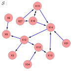
Refer to caption Refer to caption Refer to caption Refer to caption Refer to caption
Figure 5: An example of COmbINE input - output. Graph 𝒮𝒮\mathcal{S} is the actual, data-generating, underlying SMCM over 12 variables. PAGs 𝒫1,𝒫2subscript𝒫1subscript𝒫2\mathcal{P}_{1},\mathcal{P}_{2} and 𝒫3subscript𝒫3\mathcal{P}_{3} are the output of FCI ran with an oracle of conditional independence on three different marginals of 𝒢𝒢\mathcal{G}. \mathcal{H} is the output of COmbINE  algorithm. The sets of latent variables (with respect to the union of observed variables) per data set are: 𝐋1={X9}subscript𝐋1𝑋9\mathbf{L}_{1}=\{X9\}, 𝐋2={}subscript𝐋2\mathbf{L}_{2}=\{\emptyset\}, 𝐋3={X18}subscript𝐋3𝑋18\mathbf{L}_{3}=\{X18\}. The sets of manipulated variables (annotated as rectangle nodes instead of circles in the respective graphs) are: 𝐈1={X14,X34}subscript𝐈1𝑋14𝑋34\mathbf{I}_{1}=\{X14,X34\}, 𝐈2={X15,X8}subscript𝐈2𝑋15𝑋8\mathbf{I}_{2}=\{X15,X8\}, 𝐈3={X9,X12}subscript𝐈3𝑋9𝑋12\mathbf{I}_{3}=\{X9,X12\}. Notice that X10𝑋10X10 and X31𝑋31X31 are adjacent in 𝒫2subscript𝒫2\mathcal{P}_{2}, but not in 𝒫1subscript𝒫1\mathcal{P}_{1} or 𝒫3subscript𝒫3\mathcal{P}_{3}. This happens because there exists an inducing path in the underlying SMCM (X31 X14 X10𝑋31 𝑋14 𝑋10X31\raisebox{2.2pt}{ \leavevmode\hbox to14.63pt{\vbox to0.4pt{\pgfpicture\makeatletter\hbox{\hskip 0.2pt\lower-0.2pt\hbox to0.0pt{\pgfsys@beginscope\pgfsys@invoke{ }\definecolor{pgfstrokecolor}{rgb}{0,0,0}\pgfsys@color@rgb@stroke{0}{0}{0}\pgfsys@invoke{ }\pgfsys@color@rgb@fill{0}{0}{0}\pgfsys@invoke{ }\pgfsys@setlinewidth{0.4pt}\pgfsys@invoke{ }\nullfont\hbox to0.0pt{\pgfsys@beginscope\pgfsys@invoke{ }\pgfsys@setlinewidth{0.1pt}\pgfsys@invoke{ } {{}}\hbox{\hbox{{\pgfsys@beginscope\pgfsys@invoke{ }{{}{{}}{}{}} \pgfsys@invoke{\lxSVG@closescope }\pgfsys@endscope}}} {{{{}}}}{{}}\hbox{\hbox{{\pgfsys@beginscope\pgfsys@invoke{ }{{}{{}}{}{}} \pgfsys@invoke{\lxSVG@closescope }\pgfsys@endscope}}} {{}}{}{{}}{}\hbox{\hbox{{\pgfsys@beginscope\pgfsys@invoke{ }{}{{}}{}{{}} {}{}\pgfsys@beginscope\pgfsys@invoke{ }\pgfsys@setlinewidth{0.4pt}\pgfsys@invoke{ }{}{}{}{}{{}}\pgfsys@moveto{0.0pt}{0.0pt}\pgfsys@lineto{10.62643pt}{0.0pt}\pgfsys@stroke\pgfsys@invoke{ }{{}{{}}{}{}{{}}{{{}}{{{}}{\pgfsys@beginscope\pgfsys@invoke{ }\pgfsys@transformcm{1.0}{0.0}{0.0}{1.0}{10.62643pt}{0.0pt}\pgfsys@invoke{ }\pgfsys@invoke{ \lxSVG@closescope }\pgfsys@invoke{\lxSVG@closescope }\pgfsys@endscope}}{{}}}} \pgfsys@invoke{\lxSVG@closescope }\pgfsys@endscope\pgfsys@invoke{\lxSVG@closescope }\pgfsys@endscope}}} \pgfsys@invoke{\lxSVG@closescope }\pgfsys@endscope{}{}{}\hss}\pgfsys@discardpath\pgfsys@invoke{\lxSVG@closescope }\pgfsys@endscope\hss}}\lxSVG@closescope\endpgfpicture}}}X14\raisebox{2.2pt}{ \leavevmode\hbox to14.63pt{\vbox to0.4pt{\pgfpicture\makeatletter\hbox{\hskip 0.2pt\lower-0.2pt\hbox to0.0pt{\pgfsys@beginscope\pgfsys@invoke{ }\definecolor{pgfstrokecolor}{rgb}{0,0,0}\pgfsys@color@rgb@stroke{0}{0}{0}\pgfsys@invoke{ }\pgfsys@color@rgb@fill{0}{0}{0}\pgfsys@invoke{ }\pgfsys@setlinewidth{0.4pt}\pgfsys@invoke{ }\nullfont\hbox to0.0pt{\pgfsys@beginscope\pgfsys@invoke{ }\pgfsys@setlinewidth{0.1pt}\pgfsys@invoke{ } {{}}\hbox{\hbox{{\pgfsys@beginscope\pgfsys@invoke{ }{{}{{}}{}{}} \pgfsys@invoke{\lxSVG@closescope }\pgfsys@endscope}}} {{{{}}}}{{}}\hbox{\hbox{{\pgfsys@beginscope\pgfsys@invoke{ }{{}{{}}{}{}} \pgfsys@invoke{\lxSVG@closescope }\pgfsys@endscope}}} {{}}{}{{}}{}\hbox{\hbox{{\pgfsys@beginscope\pgfsys@invoke{ }{}{{}}{}{{}} {}{}\pgfsys@beginscope\pgfsys@invoke{ }\pgfsys@setlinewidth{0.4pt}\pgfsys@invoke{ }{}{}{}{}{{}}{}{}{}{{}}\pgfsys@moveto{3.59995pt}{0.0pt}\pgfsys@lineto{10.62643pt}{0.0pt}\pgfsys@stroke\pgfsys@invoke{ }{{}{{}}{}{}{{}}{{{}}{{{}}{\pgfsys@beginscope\pgfsys@invoke{ }\pgfsys@transformcm{-1.0}{0.0}{0.0}{-1.0}{3.59995pt}{0.0pt}\pgfsys@invoke{ }\pgfsys@invoke{ \lxSVG@closescope }\pgfsys@invoke{\lxSVG@closescope }\pgfsys@endscope}}{{}}}}{{}{{}}{}{}{{}}{{{}}{{{}}{\pgfsys@beginscope\pgfsys@invoke{ }\pgfsys@transformcm{1.0}{0.0}{0.0}{1.0}{10.62643pt}{0.0pt}\pgfsys@invoke{ }\pgfsys@invoke{ \lxSVG@closescope }\pgfsys@invoke{\lxSVG@closescope }\pgfsys@endscope}}{{}}}} \pgfsys@invoke{\lxSVG@closescope }\pgfsys@endscope\pgfsys@invoke{\lxSVG@closescope }\pgfsys@endscope}}} \pgfsys@invoke{\lxSVG@closescope }\pgfsys@endscope{}{}{}\hss}\pgfsys@discardpath\pgfsys@invoke{\lxSVG@closescope }\pgfsys@endscope\hss}}\lxSVG@closescope\endpgfpicture}}}X10 in 𝒮𝒮\mathcal{S}) that is “broken” by the manipulation of X14𝑋14X14 and X12𝑋12X12, respectively. Also notice a dashed edge between X9𝑋9X9 and X15𝑋15X15, which cannot be excluded since the variables have never been observed unmanipulated together. Even if the link existed, it would be destroyed in both 𝒫2subscript𝒫2\mathcal{P}_{2} and 𝒫3subscript𝒫3\mathcal{P}_{3}, where both variables are observed. All graphs were visualized in Cytoscape (Smoot et al., 2011).

without imposing the antecedent. These semantics should always be guaranteed and thus, ΦΦ\Phi forms a set of hard-constraints. In contrast, if the list of antecedents in \mathcal{F} leads to a conflict, one can select only a subset of antecedents to satisfy (soft-constraints).

Recall that the propositional variables of ΦΦ\Phi correspond to the features of the actual underlying SMCM (its edges and endpoints). Some of these variables have the same value in all the possible truth-setting assignments of ΦΦsuperscript\Phi\wedge\mathcal{F}^{\prime}, meaning the respective features are invariant in all possible underlying SMCMs. Such variables are called backbone variables of ΦΦsuperscript\Phi\wedge\mathcal{F}^{\prime} (Hyttinen et al., 2013). The actual value of a backbone variable is called the polarity of the variable. For sake of brevity, we say an edge or endpoint has polarity 0/1 if the corresponding variable is a backbone variable in ΦΦsuperscript\Phi\wedge\mathcal{F}^{\prime} and has polarity 0/1. Based on the backbone of ΦΦsuperscript\Phi\wedge\mathcal{F}^{\prime}, the final step of COmbINE  is to construct the summary graph 𝒮𝒮\mathcal{S}. 𝒮𝒮\mathcal{S} has the following types of edges and endpoints:

  • Solid Edges: in \mathcal{H} that have polarity 1 in ΦΦsuperscript\Phi\wedge\mathcal{F}^{\prime}, meaning that they are present in all possible underlying SMCM.

  • Absent Edges: Edges that are not in \mathcal{H} or edges in \mathcal{H} that have polarity 0 in ΦΦ\Phi, meaning that they are absent in all possible underlying SMCM.

  • Dashed Edges: Edges in \mathcal{H} that are not backbone variables in ΦΦsuperscript\Phi\wedge\mathcal{F}^{\prime}, meaning that there exists at least one possible underlying SMCM where this edge is present and one where this edge is absent.

  • Solid Endpoints: Endpoints in \mathcal{H} that are backbone variables in ΦΦsuperscript\Phi\wedge\mathcal{F}^{\prime}, meaning that this orientation is invariant in all possible underlying SMCMs.

  • Dashed (circled) Endpoints: Endpoints in \mathcal{H} that are not backbone variables in ΦΦsuperscript\Phi\wedge\mathcal{F}^{\prime}, meaning that there exists at least one SMCM where this orientation does not hold.

We use the term solid features of the summary graph to denote the set of solid edges, absent edges and solid endpoints of the summary graph.

Refer to caption Refer to caption Refer to caption
Figure 6: A detailed example of a non-trivial inference. From left to right: The true underlying SMCM over variables X𝑋X, Y𝑌Y, Z𝑍Z, W𝑊W; PAGs 𝒫1subscript𝒫1\mathcal{P}_{1} and 𝒫2subscript𝒫2\mathcal{P}_{2} over {X,Y,W}𝑋𝑌𝑊\{X,Y,W\} and {X,Z,W}𝑋𝑍𝑊\{X,Z,W\}, respectively; The output \mathcal{H} of Algorithm 2 ran with an oracle of conditional independence. Notice that, the edges in 𝒫1subscript𝒫1\mathcal{P}_{1} can not both simultaneously occur in a consistent SMCM 𝒮𝒮\mathcal{S}: This would make X Y W𝑋 𝑌 𝑊X\raisebox{1.0pt}{ \leavevmode\hbox to17.86pt{\vbox to3.64pt{\pgfpicture\makeatletter\hbox{\hskip 1.81783pt\lower-1.81783pt\hbox to0.0pt{\pgfsys@beginscope\pgfsys@invoke{ }\definecolor{pgfstrokecolor}{rgb}{0,0,0}\pgfsys@color@rgb@stroke{0}{0}{0}\pgfsys@invoke{ }\pgfsys@color@rgb@fill{0}{0}{0}\pgfsys@invoke{ }\pgfsys@setlinewidth{0.4pt}\pgfsys@invoke{ }\nullfont\hbox to0.0pt{\pgfsys@beginscope\pgfsys@invoke{ }\pgfsys@setlinewidth{0.1pt}\pgfsys@invoke{ } {{}}\hbox{\hbox{{\pgfsys@beginscope\pgfsys@invoke{ }{{}{{{}}}{{}}{}{}{}{}{}{}{}{}{}{{}\pgfsys@moveto{1.76782pt}{0.0pt}\pgfsys@curveto{1.76782pt}{0.97635pt}{0.97635pt}{1.76782pt}{0.0pt}{1.76782pt}\pgfsys@curveto{-0.97635pt}{1.76782pt}{-1.76782pt}{0.97635pt}{-1.76782pt}{0.0pt}\pgfsys@curveto{-1.76782pt}{-0.97635pt}{-0.97635pt}{-1.76782pt}{0.0pt}{-1.76782pt}\pgfsys@curveto{0.97635pt}{-1.76782pt}{1.76782pt}{-0.97635pt}{1.76782pt}{0.0pt}\pgfsys@closepath\pgfsys@moveto{0.0pt}{0.0pt}\pgfsys@stroke\pgfsys@invoke{ } }{{{{}}\pgfsys@beginscope\pgfsys@invoke{ }\pgfsys@transformcm{1.0}{0.0}{0.0}{1.0}{0.0pt}{0.0pt}\pgfsys@invoke{ }\hbox{{\definecolor{pgfstrokecolor}{rgb}{0,0,0}\pgfsys@color@rgb@stroke{0}{0}{0}\pgfsys@invoke{ }\pgfsys@color@rgb@fill{0}{0}{0}\pgfsys@invoke{ }\hbox{} }}\pgfsys@invoke{\lxSVG@closescope }\pgfsys@endscope}}} \pgfsys@invoke{\lxSVG@closescope }\pgfsys@endscope}}} {{{{}}}}{{}}\hbox{\hbox{{\pgfsys@beginscope\pgfsys@invoke{ }{{}{{{}}}{{}}{}{}{}{}{}{}{}{}{}{{}\pgfsys@moveto{15.9942pt}{0.0pt}\pgfsys@curveto{15.9942pt}{0.97635pt}{15.20273pt}{1.76782pt}{14.22638pt}{1.76782pt}\pgfsys@curveto{13.25003pt}{1.76782pt}{12.45856pt}{0.97635pt}{12.45856pt}{0.0pt}\pgfsys@curveto{12.45856pt}{-0.97635pt}{13.25003pt}{-1.76782pt}{14.22638pt}{-1.76782pt}\pgfsys@curveto{15.20273pt}{-1.76782pt}{15.9942pt}{-0.97635pt}{15.9942pt}{0.0pt}\pgfsys@closepath\pgfsys@moveto{14.22638pt}{0.0pt}\pgfsys@stroke\pgfsys@invoke{ } }{{{{}}\pgfsys@beginscope\pgfsys@invoke{ }\pgfsys@transformcm{1.0}{0.0}{0.0}{1.0}{14.22638pt}{0.0pt}\pgfsys@invoke{ }\hbox{{\definecolor{pgfstrokecolor}{rgb}{0,0,0}\pgfsys@color@rgb@stroke{0}{0}{0}\pgfsys@invoke{ }\pgfsys@color@rgb@fill{0}{0}{0}\pgfsys@invoke{ }\hbox{} }}\pgfsys@invoke{\lxSVG@closescope }\pgfsys@endscope}}} \pgfsys@invoke{\lxSVG@closescope }\pgfsys@endscope}}} {{}}{}\hbox{\hbox{{\pgfsys@beginscope\pgfsys@invoke{ }{{}}{}{{}} {{{{{}}{}{}{}{}{{}}}}}{}{{{{{}}{}{}{}{}{{}}}}}{{}}{}{}{}{}\pgfsys@moveto{1.81783pt}{0.0pt}\pgfsys@lineto{12.40855pt}{0.0pt}\pgfsys@stroke\pgfsys@invoke{ } \pgfsys@invoke{\lxSVG@closescope }\pgfsys@endscope}}} \pgfsys@invoke{\lxSVG@closescope }\pgfsys@endscope{}{}{}\hss}\pgfsys@discardpath\pgfsys@invoke{\lxSVG@closescope }\pgfsys@endscope\hss}}\lxSVG@closescope\endpgfpicture}}}Y\raisebox{1.0pt}{ \leavevmode\hbox to17.86pt{\vbox to3.64pt{\pgfpicture\makeatletter\hbox{\hskip 1.81783pt\lower-1.81783pt\hbox to0.0pt{\pgfsys@beginscope\pgfsys@invoke{ }\definecolor{pgfstrokecolor}{rgb}{0,0,0}\pgfsys@color@rgb@stroke{0}{0}{0}\pgfsys@invoke{ }\pgfsys@color@rgb@fill{0}{0}{0}\pgfsys@invoke{ }\pgfsys@setlinewidth{0.4pt}\pgfsys@invoke{ }\nullfont\hbox to0.0pt{\pgfsys@beginscope\pgfsys@invoke{ }\pgfsys@setlinewidth{0.1pt}\pgfsys@invoke{ } {{}}\hbox{\hbox{{\pgfsys@beginscope\pgfsys@invoke{ }{{}{{{}}}{{}}{}{}{}{}{}{}{}{}{}{{}\pgfsys@moveto{1.76782pt}{0.0pt}\pgfsys@curveto{1.76782pt}{0.97635pt}{0.97635pt}{1.76782pt}{0.0pt}{1.76782pt}\pgfsys@curveto{-0.97635pt}{1.76782pt}{-1.76782pt}{0.97635pt}{-1.76782pt}{0.0pt}\pgfsys@curveto{-1.76782pt}{-0.97635pt}{-0.97635pt}{-1.76782pt}{0.0pt}{-1.76782pt}\pgfsys@curveto{0.97635pt}{-1.76782pt}{1.76782pt}{-0.97635pt}{1.76782pt}{0.0pt}\pgfsys@closepath\pgfsys@moveto{0.0pt}{0.0pt}\pgfsys@stroke\pgfsys@invoke{ } }{{{{}}\pgfsys@beginscope\pgfsys@invoke{ }\pgfsys@transformcm{1.0}{0.0}{0.0}{1.0}{0.0pt}{0.0pt}\pgfsys@invoke{ }\hbox{{\definecolor{pgfstrokecolor}{rgb}{0,0,0}\pgfsys@color@rgb@stroke{0}{0}{0}\pgfsys@invoke{ }\pgfsys@color@rgb@fill{0}{0}{0}\pgfsys@invoke{ }\hbox{} }}\pgfsys@invoke{\lxSVG@closescope }\pgfsys@endscope}}} \pgfsys@invoke{\lxSVG@closescope }\pgfsys@endscope}}} {{{{}}}}{{}}\hbox{\hbox{{\pgfsys@beginscope\pgfsys@invoke{ }{{}{{{}}}{{}}{}{}{}{}{}{}{}{}{}{{}\pgfsys@moveto{15.9942pt}{0.0pt}\pgfsys@curveto{15.9942pt}{0.97635pt}{15.20273pt}{1.76782pt}{14.22638pt}{1.76782pt}\pgfsys@curveto{13.25003pt}{1.76782pt}{12.45856pt}{0.97635pt}{12.45856pt}{0.0pt}\pgfsys@curveto{12.45856pt}{-0.97635pt}{13.25003pt}{-1.76782pt}{14.22638pt}{-1.76782pt}\pgfsys@curveto{15.20273pt}{-1.76782pt}{15.9942pt}{-0.97635pt}{15.9942pt}{0.0pt}\pgfsys@closepath\pgfsys@moveto{14.22638pt}{0.0pt}\pgfsys@stroke\pgfsys@invoke{ } }{{{{}}\pgfsys@beginscope\pgfsys@invoke{ }\pgfsys@transformcm{1.0}{0.0}{0.0}{1.0}{14.22638pt}{0.0pt}\pgfsys@invoke{ }\hbox{{\definecolor{pgfstrokecolor}{rgb}{0,0,0}\pgfsys@color@rgb@stroke{0}{0}{0}\pgfsys@invoke{ }\pgfsys@color@rgb@fill{0}{0}{0}\pgfsys@invoke{ }\hbox{} }}\pgfsys@invoke{\lxSVG@closescope }\pgfsys@endscope}}} \pgfsys@invoke{\lxSVG@closescope }\pgfsys@endscope}}} {{}}{}\hbox{\hbox{{\pgfsys@beginscope\pgfsys@invoke{ }{{}}{}{{}} {{{{{}}{}{}{}{}{{}}}}}{}{{{{{}}{}{}{}{}{{}}}}}{{}}{}{}{}{}\pgfsys@moveto{1.81783pt}{0.0pt}\pgfsys@lineto{12.40855pt}{0.0pt}\pgfsys@stroke\pgfsys@invoke{ } \pgfsys@invoke{\lxSVG@closescope }\pgfsys@endscope}}} \pgfsys@invoke{\lxSVG@closescope }\pgfsys@endscope{}{}{}\hss}\pgfsys@discardpath\pgfsys@invoke{\lxSVG@closescope }\pgfsys@endscope\hss}}\lxSVG@closescope\endpgfpicture}}}W an inducing path for X𝑋X and W𝑊W with respect to 𝐋2={Y}subscript𝐋2𝑌\mathbf{L}_{2}=\{Y\} and contradict the features of 𝒫2subscript𝒫2\mathcal{P}_{2}, where X𝑋X and W𝑊W are not adjacent. Similarly, X Z W𝑋 𝑍 𝑊X\raisebox{1.0pt}{ \leavevmode\hbox to17.86pt{\vbox to3.64pt{\pgfpicture\makeatletter\hbox{\hskip 1.81783pt\lower-1.81783pt\hbox to0.0pt{\pgfsys@beginscope\pgfsys@invoke{ }\definecolor{pgfstrokecolor}{rgb}{0,0,0}\pgfsys@color@rgb@stroke{0}{0}{0}\pgfsys@invoke{ }\pgfsys@color@rgb@fill{0}{0}{0}\pgfsys@invoke{ }\pgfsys@setlinewidth{0.4pt}\pgfsys@invoke{ }\nullfont\hbox to0.0pt{\pgfsys@beginscope\pgfsys@invoke{ }\pgfsys@setlinewidth{0.1pt}\pgfsys@invoke{ } {{}}\hbox{\hbox{{\pgfsys@beginscope\pgfsys@invoke{ }{{}{{{}}}{{}}{}{}{}{}{}{}{}{}{}{{}\pgfsys@moveto{1.76782pt}{0.0pt}\pgfsys@curveto{1.76782pt}{0.97635pt}{0.97635pt}{1.76782pt}{0.0pt}{1.76782pt}\pgfsys@curveto{-0.97635pt}{1.76782pt}{-1.76782pt}{0.97635pt}{-1.76782pt}{0.0pt}\pgfsys@curveto{-1.76782pt}{-0.97635pt}{-0.97635pt}{-1.76782pt}{0.0pt}{-1.76782pt}\pgfsys@curveto{0.97635pt}{-1.76782pt}{1.76782pt}{-0.97635pt}{1.76782pt}{0.0pt}\pgfsys@closepath\pgfsys@moveto{0.0pt}{0.0pt}\pgfsys@stroke\pgfsys@invoke{ } }{{{{}}\pgfsys@beginscope\pgfsys@invoke{ }\pgfsys@transformcm{1.0}{0.0}{0.0}{1.0}{0.0pt}{0.0pt}\pgfsys@invoke{ }\hbox{{\definecolor{pgfstrokecolor}{rgb}{0,0,0}\pgfsys@color@rgb@stroke{0}{0}{0}\pgfsys@invoke{ }\pgfsys@color@rgb@fill{0}{0}{0}\pgfsys@invoke{ }\hbox{} }}\pgfsys@invoke{\lxSVG@closescope }\pgfsys@endscope}}} \pgfsys@invoke{\lxSVG@closescope }\pgfsys@endscope}}} {{{{}}}}{{}}\hbox{\hbox{{\pgfsys@beginscope\pgfsys@invoke{ }{{}{{{}}}{{}}{}{}{}{}{}{}{}{}{}{{}\pgfsys@moveto{15.9942pt}{0.0pt}\pgfsys@curveto{15.9942pt}{0.97635pt}{15.20273pt}{1.76782pt}{14.22638pt}{1.76782pt}\pgfsys@curveto{13.25003pt}{1.76782pt}{12.45856pt}{0.97635pt}{12.45856pt}{0.0pt}\pgfsys@curveto{12.45856pt}{-0.97635pt}{13.25003pt}{-1.76782pt}{14.22638pt}{-1.76782pt}\pgfsys@curveto{15.20273pt}{-1.76782pt}{15.9942pt}{-0.97635pt}{15.9942pt}{0.0pt}\pgfsys@closepath\pgfsys@moveto{14.22638pt}{0.0pt}\pgfsys@stroke\pgfsys@invoke{ } }{{{{}}\pgfsys@beginscope\pgfsys@invoke{ }\pgfsys@transformcm{1.0}{0.0}{0.0}{1.0}{14.22638pt}{0.0pt}\pgfsys@invoke{ }\hbox{{\definecolor{pgfstrokecolor}{rgb}{0,0,0}\pgfsys@color@rgb@stroke{0}{0}{0}\pgfsys@invoke{ }\pgfsys@color@rgb@fill{0}{0}{0}\pgfsys@invoke{ }\hbox{} }}\pgfsys@invoke{\lxSVG@closescope }\pgfsys@endscope}}} \pgfsys@invoke{\lxSVG@closescope }\pgfsys@endscope}}} {{}}{}\hbox{\hbox{{\pgfsys@beginscope\pgfsys@invoke{ }{{}}{}{{}} {{{{{}}{}{}{}{}{{}}}}}{}{{{{{}}{}{}{}{}{{}}}}}{{}}{}{}{}{}\pgfsys@moveto{1.81783pt}{0.0pt}\pgfsys@lineto{12.40855pt}{0.0pt}\pgfsys@stroke\pgfsys@invoke{ } \pgfsys@invoke{\lxSVG@closescope }\pgfsys@endscope}}} \pgfsys@invoke{\lxSVG@closescope }\pgfsys@endscope{}{}{}\hss}\pgfsys@discardpath\pgfsys@invoke{\lxSVG@closescope }\pgfsys@endscope\hss}}\lxSVG@closescope\endpgfpicture}}}Z\raisebox{1.0pt}{ \leavevmode\hbox to17.86pt{\vbox to3.64pt{\pgfpicture\makeatletter\hbox{\hskip 1.81783pt\lower-1.81783pt\hbox to0.0pt{\pgfsys@beginscope\pgfsys@invoke{ }\definecolor{pgfstrokecolor}{rgb}{0,0,0}\pgfsys@color@rgb@stroke{0}{0}{0}\pgfsys@invoke{ }\pgfsys@color@rgb@fill{0}{0}{0}\pgfsys@invoke{ }\pgfsys@setlinewidth{0.4pt}\pgfsys@invoke{ }\nullfont\hbox to0.0pt{\pgfsys@beginscope\pgfsys@invoke{ }\pgfsys@setlinewidth{0.1pt}\pgfsys@invoke{ } {{}}\hbox{\hbox{{\pgfsys@beginscope\pgfsys@invoke{ }{{}{{{}}}{{}}{}{}{}{}{}{}{}{}{}{{}\pgfsys@moveto{1.76782pt}{0.0pt}\pgfsys@curveto{1.76782pt}{0.97635pt}{0.97635pt}{1.76782pt}{0.0pt}{1.76782pt}\pgfsys@curveto{-0.97635pt}{1.76782pt}{-1.76782pt}{0.97635pt}{-1.76782pt}{0.0pt}\pgfsys@curveto{-1.76782pt}{-0.97635pt}{-0.97635pt}{-1.76782pt}{0.0pt}{-1.76782pt}\pgfsys@curveto{0.97635pt}{-1.76782pt}{1.76782pt}{-0.97635pt}{1.76782pt}{0.0pt}\pgfsys@closepath\pgfsys@moveto{0.0pt}{0.0pt}\pgfsys@stroke\pgfsys@invoke{ } }{{{{}}\pgfsys@beginscope\pgfsys@invoke{ }\pgfsys@transformcm{1.0}{0.0}{0.0}{1.0}{0.0pt}{0.0pt}\pgfsys@invoke{ }\hbox{{\definecolor{pgfstrokecolor}{rgb}{0,0,0}\pgfsys@color@rgb@stroke{0}{0}{0}\pgfsys@invoke{ }\pgfsys@color@rgb@fill{0}{0}{0}\pgfsys@invoke{ }\hbox{} }}\pgfsys@invoke{\lxSVG@closescope }\pgfsys@endscope}}} \pgfsys@invoke{\lxSVG@closescope }\pgfsys@endscope}}} {{{{}}}}{{}}\hbox{\hbox{{\pgfsys@beginscope\pgfsys@invoke{ }{{}{{{}}}{{}}{}{}{}{}{}{}{}{}{}{{}\pgfsys@moveto{15.9942pt}{0.0pt}\pgfsys@curveto{15.9942pt}{0.97635pt}{15.20273pt}{1.76782pt}{14.22638pt}{1.76782pt}\pgfsys@curveto{13.25003pt}{1.76782pt}{12.45856pt}{0.97635pt}{12.45856pt}{0.0pt}\pgfsys@curveto{12.45856pt}{-0.97635pt}{13.25003pt}{-1.76782pt}{14.22638pt}{-1.76782pt}\pgfsys@curveto{15.20273pt}{-1.76782pt}{15.9942pt}{-0.97635pt}{15.9942pt}{0.0pt}\pgfsys@closepath\pgfsys@moveto{14.22638pt}{0.0pt}\pgfsys@stroke\pgfsys@invoke{ } }{{{{}}\pgfsys@beginscope\pgfsys@invoke{ }\pgfsys@transformcm{1.0}{0.0}{0.0}{1.0}{14.22638pt}{0.0pt}\pgfsys@invoke{ }\hbox{{\definecolor{pgfstrokecolor}{rgb}{0,0,0}\pgfsys@color@rgb@stroke{0}{0}{0}\pgfsys@invoke{ }\pgfsys@color@rgb@fill{0}{0}{0}\pgfsys@invoke{ }\hbox{} }}\pgfsys@invoke{\lxSVG@closescope }\pgfsys@endscope}}} \pgfsys@invoke{\lxSVG@closescope }\pgfsys@endscope}}} {{}}{}\hbox{\hbox{{\pgfsys@beginscope\pgfsys@invoke{ }{{}}{}{{}} {{{{{}}{}{}{}{}{{}}}}}{}{{{{{}}{}{}{}{}{{}}}}}{{}}{}{}{}{}\pgfsys@moveto{1.81783pt}{0.0pt}\pgfsys@lineto{12.40855pt}{0.0pt}\pgfsys@stroke\pgfsys@invoke{ } \pgfsys@invoke{\lxSVG@closescope }\pgfsys@endscope}}} \pgfsys@invoke{\lxSVG@closescope }\pgfsys@endscope{}{}{}\hss}\pgfsys@discardpath\pgfsys@invoke{\lxSVG@closescope }\pgfsys@endscope\hss}}\lxSVG@closescope\endpgfpicture}}}W cannot occur in any consistent SMCM 𝒮𝒮\mathcal{S}. The only possible edge structures that explain all the observed adjacencies and definite non colliders are X Y Z W𝑋 𝑌 𝑍 𝑊X\raisebox{1.0pt}{ \leavevmode\hbox to17.86pt{\vbox to3.64pt{\pgfpicture\makeatletter\hbox{\hskip 1.81783pt\lower-1.81783pt\hbox to0.0pt{\pgfsys@beginscope\pgfsys@invoke{ }\definecolor{pgfstrokecolor}{rgb}{0,0,0}\pgfsys@color@rgb@stroke{0}{0}{0}\pgfsys@invoke{ }\pgfsys@color@rgb@fill{0}{0}{0}\pgfsys@invoke{ }\pgfsys@setlinewidth{0.4pt}\pgfsys@invoke{ }\nullfont\hbox to0.0pt{\pgfsys@beginscope\pgfsys@invoke{ }\pgfsys@setlinewidth{0.1pt}\pgfsys@invoke{ } {{}}\hbox{\hbox{{\pgfsys@beginscope\pgfsys@invoke{ }{{}{{{}}}{{}}{}{}{}{}{}{}{}{}{}{{}\pgfsys@moveto{1.76782pt}{0.0pt}\pgfsys@curveto{1.76782pt}{0.97635pt}{0.97635pt}{1.76782pt}{0.0pt}{1.76782pt}\pgfsys@curveto{-0.97635pt}{1.76782pt}{-1.76782pt}{0.97635pt}{-1.76782pt}{0.0pt}\pgfsys@curveto{-1.76782pt}{-0.97635pt}{-0.97635pt}{-1.76782pt}{0.0pt}{-1.76782pt}\pgfsys@curveto{0.97635pt}{-1.76782pt}{1.76782pt}{-0.97635pt}{1.76782pt}{0.0pt}\pgfsys@closepath\pgfsys@moveto{0.0pt}{0.0pt}\pgfsys@stroke\pgfsys@invoke{ } }{{{{}}\pgfsys@beginscope\pgfsys@invoke{ }\pgfsys@transformcm{1.0}{0.0}{0.0}{1.0}{0.0pt}{0.0pt}\pgfsys@invoke{ }\hbox{{\definecolor{pgfstrokecolor}{rgb}{0,0,0}\pgfsys@color@rgb@stroke{0}{0}{0}\pgfsys@invoke{ }\pgfsys@color@rgb@fill{0}{0}{0}\pgfsys@invoke{ }\hbox{} }}\pgfsys@invoke{\lxSVG@closescope }\pgfsys@endscope}}} \pgfsys@invoke{\lxSVG@closescope }\pgfsys@endscope}}} {{{{}}}}{{}}\hbox{\hbox{{\pgfsys@beginscope\pgfsys@invoke{ }{{}{{{}}}{{}}{}{}{}{}{}{}{}{}{}{{}\pgfsys@moveto{15.9942pt}{0.0pt}\pgfsys@curveto{15.9942pt}{0.97635pt}{15.20273pt}{1.76782pt}{14.22638pt}{1.76782pt}\pgfsys@curveto{13.25003pt}{1.76782pt}{12.45856pt}{0.97635pt}{12.45856pt}{0.0pt}\pgfsys@curveto{12.45856pt}{-0.97635pt}{13.25003pt}{-1.76782pt}{14.22638pt}{-1.76782pt}\pgfsys@curveto{15.20273pt}{-1.76782pt}{15.9942pt}{-0.97635pt}{15.9942pt}{0.0pt}\pgfsys@closepath\pgfsys@moveto{14.22638pt}{0.0pt}\pgfsys@stroke\pgfsys@invoke{ } }{{{{}}\pgfsys@beginscope\pgfsys@invoke{ }\pgfsys@transformcm{1.0}{0.0}{0.0}{1.0}{14.22638pt}{0.0pt}\pgfsys@invoke{ }\hbox{{\definecolor{pgfstrokecolor}{rgb}{0,0,0}\pgfsys@color@rgb@stroke{0}{0}{0}\pgfsys@invoke{ }\pgfsys@color@rgb@fill{0}{0}{0}\pgfsys@invoke{ }\hbox{} }}\pgfsys@invoke{\lxSVG@closescope }\pgfsys@endscope}}} \pgfsys@invoke{\lxSVG@closescope }\pgfsys@endscope}}} {{}}{}\hbox{\hbox{{\pgfsys@beginscope\pgfsys@invoke{ }{{}}{}{{}} {{{{{}}{}{}{}{}{{}}}}}{}{{{{{}}{}{}{}{}{{}}}}}{{}}{}{}{}{}\pgfsys@moveto{1.81783pt}{0.0pt}\pgfsys@lineto{12.40855pt}{0.0pt}\pgfsys@stroke\pgfsys@invoke{ } \pgfsys@invoke{\lxSVG@closescope }\pgfsys@endscope}}} \pgfsys@invoke{\lxSVG@closescope }\pgfsys@endscope{}{}{}\hss}\pgfsys@discardpath\pgfsys@invoke{\lxSVG@closescope }\pgfsys@endscope\hss}}\lxSVG@closescope\endpgfpicture}}}Y\raisebox{1.0pt}{ \leavevmode\hbox to17.86pt{\vbox to3.64pt{\pgfpicture\makeatletter\hbox{\hskip 1.81783pt\lower-1.81783pt\hbox to0.0pt{\pgfsys@beginscope\pgfsys@invoke{ }\definecolor{pgfstrokecolor}{rgb}{0,0,0}\pgfsys@color@rgb@stroke{0}{0}{0}\pgfsys@invoke{ }\pgfsys@color@rgb@fill{0}{0}{0}\pgfsys@invoke{ }\pgfsys@setlinewidth{0.4pt}\pgfsys@invoke{ }\nullfont\hbox to0.0pt{\pgfsys@beginscope\pgfsys@invoke{ }\pgfsys@setlinewidth{0.1pt}\pgfsys@invoke{ } {{}}\hbox{\hbox{{\pgfsys@beginscope\pgfsys@invoke{ }{{}{{{}}}{{}}{}{}{}{}{}{}{}{}{}{{}\pgfsys@moveto{1.76782pt}{0.0pt}\pgfsys@curveto{1.76782pt}{0.97635pt}{0.97635pt}{1.76782pt}{0.0pt}{1.76782pt}\pgfsys@curveto{-0.97635pt}{1.76782pt}{-1.76782pt}{0.97635pt}{-1.76782pt}{0.0pt}\pgfsys@curveto{-1.76782pt}{-0.97635pt}{-0.97635pt}{-1.76782pt}{0.0pt}{-1.76782pt}\pgfsys@curveto{0.97635pt}{-1.76782pt}{1.76782pt}{-0.97635pt}{1.76782pt}{0.0pt}\pgfsys@closepath\pgfsys@moveto{0.0pt}{0.0pt}\pgfsys@stroke\pgfsys@invoke{ } }{{{{}}\pgfsys@beginscope\pgfsys@invoke{ }\pgfsys@transformcm{1.0}{0.0}{0.0}{1.0}{0.0pt}{0.0pt}\pgfsys@invoke{ }\hbox{{\definecolor{pgfstrokecolor}{rgb}{0,0,0}\pgfsys@color@rgb@stroke{0}{0}{0}\pgfsys@invoke{ }\pgfsys@color@rgb@fill{0}{0}{0}\pgfsys@invoke{ }\hbox{} }}\pgfsys@invoke{\lxSVG@closescope }\pgfsys@endscope}}} \pgfsys@invoke{\lxSVG@closescope }\pgfsys@endscope}}} {{{{}}}}{{}}\hbox{\hbox{{\pgfsys@beginscope\pgfsys@invoke{ }{{}{{{}}}{{}}{}{}{}{}{}{}{}{}{}{{}\pgfsys@moveto{15.9942pt}{0.0pt}\pgfsys@curveto{15.9942pt}{0.97635pt}{15.20273pt}{1.76782pt}{14.22638pt}{1.76782pt}\pgfsys@curveto{13.25003pt}{1.76782pt}{12.45856pt}{0.97635pt}{12.45856pt}{0.0pt}\pgfsys@curveto{12.45856pt}{-0.97635pt}{13.25003pt}{-1.76782pt}{14.22638pt}{-1.76782pt}\pgfsys@curveto{15.20273pt}{-1.76782pt}{15.9942pt}{-0.97635pt}{15.9942pt}{0.0pt}\pgfsys@closepath\pgfsys@moveto{14.22638pt}{0.0pt}\pgfsys@stroke\pgfsys@invoke{ } }{{{{}}\pgfsys@beginscope\pgfsys@invoke{ }\pgfsys@transformcm{1.0}{0.0}{0.0}{1.0}{14.22638pt}{0.0pt}\pgfsys@invoke{ }\hbox{{\definecolor{pgfstrokecolor}{rgb}{0,0,0}\pgfsys@color@rgb@stroke{0}{0}{0}\pgfsys@invoke{ }\pgfsys@color@rgb@fill{0}{0}{0}\pgfsys@invoke{ }\hbox{} }}\pgfsys@invoke{\lxSVG@closescope }\pgfsys@endscope}}} \pgfsys@invoke{\lxSVG@closescope }\pgfsys@endscope}}} {{}}{}\hbox{\hbox{{\pgfsys@beginscope\pgfsys@invoke{ }{{}}{}{{}} {{{{{}}{}{}{}{}{{}}}}}{}{{{{{}}{}{}{}{}{{}}}}}{{}}{}{}{}{}\pgfsys@moveto{1.81783pt}{0.0pt}\pgfsys@lineto{12.40855pt}{0.0pt}\pgfsys@stroke\pgfsys@invoke{ } \pgfsys@invoke{\lxSVG@closescope }\pgfsys@endscope}}} \pgfsys@invoke{\lxSVG@closescope }\pgfsys@endscope{}{}{}\hss}\pgfsys@discardpath\pgfsys@invoke{\lxSVG@closescope }\pgfsys@endscope\hss}}\lxSVG@closescope\endpgfpicture}}}Z\raisebox{1.0pt}{ \leavevmode\hbox to17.86pt{\vbox to3.64pt{\pgfpicture\makeatletter\hbox{\hskip 1.81783pt\lower-1.81783pt\hbox to0.0pt{\pgfsys@beginscope\pgfsys@invoke{ }\definecolor{pgfstrokecolor}{rgb}{0,0,0}\pgfsys@color@rgb@stroke{0}{0}{0}\pgfsys@invoke{ }\pgfsys@color@rgb@fill{0}{0}{0}\pgfsys@invoke{ }\pgfsys@setlinewidth{0.4pt}\pgfsys@invoke{ }\nullfont\hbox to0.0pt{\pgfsys@beginscope\pgfsys@invoke{ }\pgfsys@setlinewidth{0.1pt}\pgfsys@invoke{ } {{}}\hbox{\hbox{{\pgfsys@beginscope\pgfsys@invoke{ }{{}{{{}}}{{}}{}{}{}{}{}{}{}{}{}{{}\pgfsys@moveto{1.76782pt}{0.0pt}\pgfsys@curveto{1.76782pt}{0.97635pt}{0.97635pt}{1.76782pt}{0.0pt}{1.76782pt}\pgfsys@curveto{-0.97635pt}{1.76782pt}{-1.76782pt}{0.97635pt}{-1.76782pt}{0.0pt}\pgfsys@curveto{-1.76782pt}{-0.97635pt}{-0.97635pt}{-1.76782pt}{0.0pt}{-1.76782pt}\pgfsys@curveto{0.97635pt}{-1.76782pt}{1.76782pt}{-0.97635pt}{1.76782pt}{0.0pt}\pgfsys@closepath\pgfsys@moveto{0.0pt}{0.0pt}\pgfsys@stroke\pgfsys@invoke{ } }{{{{}}\pgfsys@beginscope\pgfsys@invoke{ }\pgfsys@transformcm{1.0}{0.0}{0.0}{1.0}{0.0pt}{0.0pt}\pgfsys@invoke{ }\hbox{{\definecolor{pgfstrokecolor}{rgb}{0,0,0}\pgfsys@color@rgb@stroke{0}{0}{0}\pgfsys@invoke{ }\pgfsys@color@rgb@fill{0}{0}{0}\pgfsys@invoke{ }\hbox{} }}\pgfsys@invoke{\lxSVG@closescope }\pgfsys@endscope}}} \pgfsys@invoke{\lxSVG@closescope }\pgfsys@endscope}}} {{{{}}}}{{}}\hbox{\hbox{{\pgfsys@beginscope\pgfsys@invoke{ }{{}{{{}}}{{}}{}{}{}{}{}{}{}{}{}{{}\pgfsys@moveto{15.9942pt}{0.0pt}\pgfsys@curveto{15.9942pt}{0.97635pt}{15.20273pt}{1.76782pt}{14.22638pt}{1.76782pt}\pgfsys@curveto{13.25003pt}{1.76782pt}{12.45856pt}{0.97635pt}{12.45856pt}{0.0pt}\pgfsys@curveto{12.45856pt}{-0.97635pt}{13.25003pt}{-1.76782pt}{14.22638pt}{-1.76782pt}\pgfsys@curveto{15.20273pt}{-1.76782pt}{15.9942pt}{-0.97635pt}{15.9942pt}{0.0pt}\pgfsys@closepath\pgfsys@moveto{14.22638pt}{0.0pt}\pgfsys@stroke\pgfsys@invoke{ } }{{{{}}\pgfsys@beginscope\pgfsys@invoke{ }\pgfsys@transformcm{1.0}{0.0}{0.0}{1.0}{14.22638pt}{0.0pt}\pgfsys@invoke{ }\hbox{{\definecolor{pgfstrokecolor}{rgb}{0,0,0}\pgfsys@color@rgb@stroke{0}{0}{0}\pgfsys@invoke{ }\pgfsys@color@rgb@fill{0}{0}{0}\pgfsys@invoke{ }\hbox{} }}\pgfsys@invoke{\lxSVG@closescope }\pgfsys@endscope}}} \pgfsys@invoke{\lxSVG@closescope }\pgfsys@endscope}}} {{}}{}\hbox{\hbox{{\pgfsys@beginscope\pgfsys@invoke{ }{{}}{}{{}} {{{{{}}{}{}{}{}{{}}}}}{}{{{{{}}{}{}{}{}{{}}}}}{{}}{}{}{}{}\pgfsys@moveto{1.81783pt}{0.0pt}\pgfsys@lineto{12.40855pt}{0.0pt}\pgfsys@stroke\pgfsys@invoke{ } \pgfsys@invoke{\lxSVG@closescope }\pgfsys@endscope}}} \pgfsys@invoke{\lxSVG@closescope }\pgfsys@endscope{}{}{}\hss}\pgfsys@discardpath\pgfsys@invoke{\lxSVG@closescope }\pgfsys@endscope\hss}}\lxSVG@closescope\endpgfpicture}}}W or X Z Y W𝑋 𝑍 𝑌 𝑊X\raisebox{1.0pt}{ \leavevmode\hbox to17.86pt{\vbox to3.64pt{\pgfpicture\makeatletter\hbox{\hskip 1.81783pt\lower-1.81783pt\hbox to0.0pt{\pgfsys@beginscope\pgfsys@invoke{ }\definecolor{pgfstrokecolor}{rgb}{0,0,0}\pgfsys@color@rgb@stroke{0}{0}{0}\pgfsys@invoke{ }\pgfsys@color@rgb@fill{0}{0}{0}\pgfsys@invoke{ }\pgfsys@setlinewidth{0.4pt}\pgfsys@invoke{ }\nullfont\hbox to0.0pt{\pgfsys@beginscope\pgfsys@invoke{ }\pgfsys@setlinewidth{0.1pt}\pgfsys@invoke{ } {{}}\hbox{\hbox{{\pgfsys@beginscope\pgfsys@invoke{ }{{}{{{}}}{{}}{}{}{}{}{}{}{}{}{}{{}\pgfsys@moveto{1.76782pt}{0.0pt}\pgfsys@curveto{1.76782pt}{0.97635pt}{0.97635pt}{1.76782pt}{0.0pt}{1.76782pt}\pgfsys@curveto{-0.97635pt}{1.76782pt}{-1.76782pt}{0.97635pt}{-1.76782pt}{0.0pt}\pgfsys@curveto{-1.76782pt}{-0.97635pt}{-0.97635pt}{-1.76782pt}{0.0pt}{-1.76782pt}\pgfsys@curveto{0.97635pt}{-1.76782pt}{1.76782pt}{-0.97635pt}{1.76782pt}{0.0pt}\pgfsys@closepath\pgfsys@moveto{0.0pt}{0.0pt}\pgfsys@stroke\pgfsys@invoke{ } }{{{{}}\pgfsys@beginscope\pgfsys@invoke{ }\pgfsys@transformcm{1.0}{0.0}{0.0}{1.0}{0.0pt}{0.0pt}\pgfsys@invoke{ }\hbox{{\definecolor{pgfstrokecolor}{rgb}{0,0,0}\pgfsys@color@rgb@stroke{0}{0}{0}\pgfsys@invoke{ }\pgfsys@color@rgb@fill{0}{0}{0}\pgfsys@invoke{ }\hbox{} }}\pgfsys@invoke{\lxSVG@closescope }\pgfsys@endscope}}} \pgfsys@invoke{\lxSVG@closescope }\pgfsys@endscope}}} {{{{}}}}{{}}\hbox{\hbox{{\pgfsys@beginscope\pgfsys@invoke{ }{{}{{{}}}{{}}{}{}{}{}{}{}{}{}{}{{}\pgfsys@moveto{15.9942pt}{0.0pt}\pgfsys@curveto{15.9942pt}{0.97635pt}{15.20273pt}{1.76782pt}{14.22638pt}{1.76782pt}\pgfsys@curveto{13.25003pt}{1.76782pt}{12.45856pt}{0.97635pt}{12.45856pt}{0.0pt}\pgfsys@curveto{12.45856pt}{-0.97635pt}{13.25003pt}{-1.76782pt}{14.22638pt}{-1.76782pt}\pgfsys@curveto{15.20273pt}{-1.76782pt}{15.9942pt}{-0.97635pt}{15.9942pt}{0.0pt}\pgfsys@closepath\pgfsys@moveto{14.22638pt}{0.0pt}\pgfsys@stroke\pgfsys@invoke{ } }{{{{}}\pgfsys@beginscope\pgfsys@invoke{ }\pgfsys@transformcm{1.0}{0.0}{0.0}{1.0}{14.22638pt}{0.0pt}\pgfsys@invoke{ }\hbox{{\definecolor{pgfstrokecolor}{rgb}{0,0,0}\pgfsys@color@rgb@stroke{0}{0}{0}\pgfsys@invoke{ }\pgfsys@color@rgb@fill{0}{0}{0}\pgfsys@invoke{ }\hbox{} }}\pgfsys@invoke{\lxSVG@closescope }\pgfsys@endscope}}} \pgfsys@invoke{\lxSVG@closescope }\pgfsys@endscope}}} {{}}{}\hbox{\hbox{{\pgfsys@beginscope\pgfsys@invoke{ }{{}}{}{{}} {{{{{}}{}{}{}{}{{}}}}}{}{{{{{}}{}{}{}{}{{}}}}}{{}}{}{}{}{}\pgfsys@moveto{1.81783pt}{0.0pt}\pgfsys@lineto{12.40855pt}{0.0pt}\pgfsys@stroke\pgfsys@invoke{ } \pgfsys@invoke{\lxSVG@closescope }\pgfsys@endscope}}} \pgfsys@invoke{\lxSVG@closescope }\pgfsys@endscope{}{}{}\hss}\pgfsys@discardpath\pgfsys@invoke{\lxSVG@closescope }\pgfsys@endscope\hss}}\lxSVG@closescope\endpgfpicture}}}Z\raisebox{1.0pt}{ \leavevmode\hbox to17.86pt{\vbox to3.64pt{\pgfpicture\makeatletter\hbox{\hskip 1.81783pt\lower-1.81783pt\hbox to0.0pt{\pgfsys@beginscope\pgfsys@invoke{ }\definecolor{pgfstrokecolor}{rgb}{0,0,0}\pgfsys@color@rgb@stroke{0}{0}{0}\pgfsys@invoke{ }\pgfsys@color@rgb@fill{0}{0}{0}\pgfsys@invoke{ }\pgfsys@setlinewidth{0.4pt}\pgfsys@invoke{ }\nullfont\hbox to0.0pt{\pgfsys@beginscope\pgfsys@invoke{ }\pgfsys@setlinewidth{0.1pt}\pgfsys@invoke{ } {{}}\hbox{\hbox{{\pgfsys@beginscope\pgfsys@invoke{ }{{}{{{}}}{{}}{}{}{}{}{}{}{}{}{}{{}\pgfsys@moveto{1.76782pt}{0.0pt}\pgfsys@curveto{1.76782pt}{0.97635pt}{0.97635pt}{1.76782pt}{0.0pt}{1.76782pt}\pgfsys@curveto{-0.97635pt}{1.76782pt}{-1.76782pt}{0.97635pt}{-1.76782pt}{0.0pt}\pgfsys@curveto{-1.76782pt}{-0.97635pt}{-0.97635pt}{-1.76782pt}{0.0pt}{-1.76782pt}\pgfsys@curveto{0.97635pt}{-1.76782pt}{1.76782pt}{-0.97635pt}{1.76782pt}{0.0pt}\pgfsys@closepath\pgfsys@moveto{0.0pt}{0.0pt}\pgfsys@stroke\pgfsys@invoke{ } }{{{{}}\pgfsys@beginscope\pgfsys@invoke{ }\pgfsys@transformcm{1.0}{0.0}{0.0}{1.0}{0.0pt}{0.0pt}\pgfsys@invoke{ }\hbox{{\definecolor{pgfstrokecolor}{rgb}{0,0,0}\pgfsys@color@rgb@stroke{0}{0}{0}\pgfsys@invoke{ }\pgfsys@color@rgb@fill{0}{0}{0}\pgfsys@invoke{ }\hbox{} }}\pgfsys@invoke{\lxSVG@closescope }\pgfsys@endscope}}} \pgfsys@invoke{\lxSVG@closescope }\pgfsys@endscope}}} {{{{}}}}{{}}\hbox{\hbox{{\pgfsys@beginscope\pgfsys@invoke{ }{{}{{{}}}{{}}{}{}{}{}{}{}{}{}{}{{}\pgfsys@moveto{15.9942pt}{0.0pt}\pgfsys@curveto{15.9942pt}{0.97635pt}{15.20273pt}{1.76782pt}{14.22638pt}{1.76782pt}\pgfsys@curveto{13.25003pt}{1.76782pt}{12.45856pt}{0.97635pt}{12.45856pt}{0.0pt}\pgfsys@curveto{12.45856pt}{-0.97635pt}{13.25003pt}{-1.76782pt}{14.22638pt}{-1.76782pt}\pgfsys@curveto{15.20273pt}{-1.76782pt}{15.9942pt}{-0.97635pt}{15.9942pt}{0.0pt}\pgfsys@closepath\pgfsys@moveto{14.22638pt}{0.0pt}\pgfsys@stroke\pgfsys@invoke{ } }{{{{}}\pgfsys@beginscope\pgfsys@invoke{ }\pgfsys@transformcm{1.0}{0.0}{0.0}{1.0}{14.22638pt}{0.0pt}\pgfsys@invoke{ }\hbox{{\definecolor{pgfstrokecolor}{rgb}{0,0,0}\pgfsys@color@rgb@stroke{0}{0}{0}\pgfsys@invoke{ }\pgfsys@color@rgb@fill{0}{0}{0}\pgfsys@invoke{ }\hbox{} }}\pgfsys@invoke{\lxSVG@closescope }\pgfsys@endscope}}} \pgfsys@invoke{\lxSVG@closescope }\pgfsys@endscope}}} {{}}{}\hbox{\hbox{{\pgfsys@beginscope\pgfsys@invoke{ }{{}}{}{{}} {{{{{}}{}{}{}{}{{}}}}}{}{{{{{}}{}{}{}{}{{}}}}}{{}}{}{}{}{}\pgfsys@moveto{1.81783pt}{0.0pt}\pgfsys@lineto{12.40855pt}{0.0pt}\pgfsys@stroke\pgfsys@invoke{ } \pgfsys@invoke{\lxSVG@closescope }\pgfsys@endscope}}} \pgfsys@invoke{\lxSVG@closescope }\pgfsys@endscope{}{}{}\hss}\pgfsys@discardpath\pgfsys@invoke{\lxSVG@closescope }\pgfsys@endscope\hss}}\lxSVG@closescope\endpgfpicture}}}Y\raisebox{1.0pt}{ \leavevmode\hbox to17.86pt{\vbox to3.64pt{\pgfpicture\makeatletter\hbox{\hskip 1.81783pt\lower-1.81783pt\hbox to0.0pt{\pgfsys@beginscope\pgfsys@invoke{ }\definecolor{pgfstrokecolor}{rgb}{0,0,0}\pgfsys@color@rgb@stroke{0}{0}{0}\pgfsys@invoke{ }\pgfsys@color@rgb@fill{0}{0}{0}\pgfsys@invoke{ }\pgfsys@setlinewidth{0.4pt}\pgfsys@invoke{ }\nullfont\hbox to0.0pt{\pgfsys@beginscope\pgfsys@invoke{ }\pgfsys@setlinewidth{0.1pt}\pgfsys@invoke{ } {{}}\hbox{\hbox{{\pgfsys@beginscope\pgfsys@invoke{ }{{}{{{}}}{{}}{}{}{}{}{}{}{}{}{}{{}\pgfsys@moveto{1.76782pt}{0.0pt}\pgfsys@curveto{1.76782pt}{0.97635pt}{0.97635pt}{1.76782pt}{0.0pt}{1.76782pt}\pgfsys@curveto{-0.97635pt}{1.76782pt}{-1.76782pt}{0.97635pt}{-1.76782pt}{0.0pt}\pgfsys@curveto{-1.76782pt}{-0.97635pt}{-0.97635pt}{-1.76782pt}{0.0pt}{-1.76782pt}\pgfsys@curveto{0.97635pt}{-1.76782pt}{1.76782pt}{-0.97635pt}{1.76782pt}{0.0pt}\pgfsys@closepath\pgfsys@moveto{0.0pt}{0.0pt}\pgfsys@stroke\pgfsys@invoke{ } }{{{{}}\pgfsys@beginscope\pgfsys@invoke{ }\pgfsys@transformcm{1.0}{0.0}{0.0}{1.0}{0.0pt}{0.0pt}\pgfsys@invoke{ }\hbox{{\definecolor{pgfstrokecolor}{rgb}{0,0,0}\pgfsys@color@rgb@stroke{0}{0}{0}\pgfsys@invoke{ }\pgfsys@color@rgb@fill{0}{0}{0}\pgfsys@invoke{ }\hbox{} }}\pgfsys@invoke{\lxSVG@closescope }\pgfsys@endscope}}} \pgfsys@invoke{\lxSVG@closescope }\pgfsys@endscope}}} {{{{}}}}{{}}\hbox{\hbox{{\pgfsys@beginscope\pgfsys@invoke{ }{{}{{{}}}{{}}{}{}{}{}{}{}{}{}{}{{}\pgfsys@moveto{15.9942pt}{0.0pt}\pgfsys@curveto{15.9942pt}{0.97635pt}{15.20273pt}{1.76782pt}{14.22638pt}{1.76782pt}\pgfsys@curveto{13.25003pt}{1.76782pt}{12.45856pt}{0.97635pt}{12.45856pt}{0.0pt}\pgfsys@curveto{12.45856pt}{-0.97635pt}{13.25003pt}{-1.76782pt}{14.22638pt}{-1.76782pt}\pgfsys@curveto{15.20273pt}{-1.76782pt}{15.9942pt}{-0.97635pt}{15.9942pt}{0.0pt}\pgfsys@closepath\pgfsys@moveto{14.22638pt}{0.0pt}\pgfsys@stroke\pgfsys@invoke{ } }{{{{}}\pgfsys@beginscope\pgfsys@invoke{ }\pgfsys@transformcm{1.0}{0.0}{0.0}{1.0}{14.22638pt}{0.0pt}\pgfsys@invoke{ }\hbox{{\definecolor{pgfstrokecolor}{rgb}{0,0,0}\pgfsys@color@rgb@stroke{0}{0}{0}\pgfsys@invoke{ }\pgfsys@color@rgb@fill{0}{0}{0}\pgfsys@invoke{ }\hbox{} }}\pgfsys@invoke{\lxSVG@closescope }\pgfsys@endscope}}} \pgfsys@invoke{\lxSVG@closescope }\pgfsys@endscope}}} {{}}{}\hbox{\hbox{{\pgfsys@beginscope\pgfsys@invoke{ }{{}}{}{{}} {{{{{}}{}{}{}{}{{}}}}}{}{{{{{}}{}{}{}{}{{}}}}}{{}}{}{}{}{}\pgfsys@moveto{1.81783pt}{0.0pt}\pgfsys@lineto{12.40855pt}{0.0pt}\pgfsys@stroke\pgfsys@invoke{ } \pgfsys@invoke{\lxSVG@closescope }\pgfsys@endscope}}} \pgfsys@invoke{\lxSVG@closescope }\pgfsys@endscope{}{}{}\hss}\pgfsys@discardpath\pgfsys@invoke{\lxSVG@closescope }\pgfsys@endscope\hss}}\lxSVG@closescope\endpgfpicture}}}W. Either way, Y𝑌Y and Z𝑍Z share an edge in all consistent SMCMs, and the algorithm will predict a solid edge between Y𝑌Y and Z𝑍Z, even if the two have not been measured in the same data set. This example is discussed in detail in (Tsamardinos et al., 2012).

Overall, Algorithm 2 takes as input a set of data sets and a list of parameters and outputs a summary graph that has all invariant edges and orientations of the SMCMs that satisfy as many constraints as possible (according to some strategy). The algorithm is capable of non-trivial inferences, like for example the presence of a solid edge among variables never measured together. Figures 5 and 6 illustrate the output of Algorithm 2, along with the corresponding input PAGs. For an oracle of conditional independence, Algorithm 2 is sound and complete in the manner described in Theorem 13. Lemmas 10 to 12 are necessary for the proof of soundness and completeness: Lemma 10 proves that the possibly inducing and ancestral paths employed by COmbINE  are complete: for any consistent 𝒮𝒮\mathcal{S}, if p𝑝p is a path that is inducing with respect to a set 𝐋𝐋\mathbf{L} (ancestral) in 𝒮𝒮\mathcal{S}, p𝑝p is possibly inducing with respect to 𝐋𝐋\mathbf{L} (possibly ancestal) in the initial search graph \mathcal{H}, and will therefore be considered during Algorithm 4. This also implies that if there exists no possibly inducing (ancestral) path in \mathcal{H} there exists no inducing (ancestral) in 𝒮𝒮\mathcal{S}. Lemma 11 proves that any consistent SMCM 𝒮𝒮\mathcal{S} satisfies the final formula ΦFΦsuperscript𝐹\Phi\wedge F^{\prime} of Algorithm 2, and Lemma 12 proves that any truth-setting assignment of the final formula ΦFΦsuperscript𝐹\Phi\wedge F^{\prime} corresponds to a consistent SMCM 𝒮𝒮\mathcal{S}.

Lemma 10

Let {𝒫i}i=1Nsuperscriptsubscriptsubscript𝒫𝑖𝑖1𝑁\{\mathcal{P}_{i}\}_{i=1}^{N} be a set of PAGs and 𝒮𝒮\mathcal{S} a SMCM such that 𝒮𝒮\mathcal{S} is possibly underlying for {𝒫i}i=1Nsuperscriptsubscriptsubscript𝒫𝑖𝑖1𝑁\{\mathcal{P}_{i}\}_{i=1}^{N}, and let \mathcal{H} be the initial search graph returned by Algorithm 3 for {𝒫i}i=1Nsuperscriptsubscriptsubscript𝒫𝑖𝑖1𝑁\{\mathcal{P}_{i}\}_{i=1}^{N}. Then, if p𝑝p is an ancestral path in 𝒮𝒮\mathcal{S}, then p𝑝p is a possibly ancestral path in \mathcal{H}. Similarly, if p𝑝p is a possibly inducing path with respect to 𝐋𝐋\mathbf{L} in 𝒮𝒮\mathcal{S}, then p𝑝p is a possibly inducing path with respect to 𝐋𝐋\mathbf{L} in \mathcal{H}.

Proof  See Appendix Appendix A..  

Lemma 11

Let {𝐃i}i=1Nsuperscriptsubscriptsubscript𝐃𝑖𝑖1𝑁\{\mathbf{D}_{i}\}_{i=1}^{N} be a set of data sets over overlapping subsets of 𝐎𝐎\mathbf{O}, and {𝐈i}i=1Nsuperscriptsubscriptsubscript𝐈𝑖𝑖1𝑁\{\mathbf{I}_{i}\}_{i=1}^{N} be a set of (possibly empty) intervention targets such that 𝐈i𝐎isubscript𝐈𝑖subscript𝐎𝑖\mathbf{I}_{i}\subset\mathbf{O}_{i} for each i. Let 𝒫isubscript𝒫𝑖\mathcal{P}_{i} be output PAG of FCI for data set 𝐃isubscript𝐃𝑖\mathbf{D}_{i}, ΦΦsuperscript\Phi\wedge\mathcal{F}^{\prime} be the final formula of Algorithm 2, and 𝒮𝒮\mathcal{S} be a possibly underlying SMCM for {𝐏i}i=1Nsuperscriptsubscriptsubscript𝐏𝑖𝑖1𝑁\{\mathbf{P}_{i}\}_{i=1}^{N}. Then 𝒮𝒮\mathcal{S} satisfies ΦΦsuperscript\Phi\wedge\mathcal{F}^{\prime} .

Proof  See Appendix Appendix A..  

Lemma 12

Let {𝐃i}i=1Nsuperscriptsubscriptsubscript𝐃𝑖𝑖1𝑁\{\mathbf{D}_{i}\}_{i=1}^{N}, {𝐈i}i=1Nsuperscriptsubscriptsubscript𝐈𝑖𝑖1𝑁\{\mathbf{I}_{i}\}_{i=1}^{N}, {𝐏i}i=1Nsuperscriptsubscriptsubscript𝐏𝑖𝑖1𝑁\{\mathbf{P}_{i}\}_{i=1}^{N}, ΦΦsuperscript\Phi\wedge\mathcal{F}^{\prime} be defined as in Lemma 11. If graph S satisfies ΦΦsuperscript\Phi\wedge\mathcal{F}^{\prime}, then 𝒮𝒮\mathcal{S} is a possibly underlying SMCM for {𝐏i}i=1Nsuperscriptsubscriptsubscript𝐏𝑖𝑖1𝑁\{\mathbf{P}_{i}\}_{i=1}^{N}.

Proof  See Appendix Appendix A..  

Theorem 13

(Soundness and completeness of Algorithm 2) Let {𝐃i}i=1Nsuperscriptsubscriptsubscript𝐃𝑖𝑖1𝑁\{\mathbf{D}_{i}\}_{i=1}^{N}, {𝐈i}i=1Nsuperscriptsubscriptsubscript𝐈𝑖𝑖1𝑁\{\mathbf{I}_{i}\}_{i=1}^{N}, {𝐏i}i=1Nsuperscriptsubscriptsubscript𝐏𝑖𝑖1𝑁\{\mathbf{P}_{i}\}_{i=1}^{N}, ΦΦsuperscript\Phi\wedge\mathcal{F}^{\prime} be defined as in Lemma 11. Finally, let \mathcal{H} be the summary graph returned by COmbINE . Then the following hold:
Soundness: If a feature (edge, absent edge, endpoint) is solid in \mathcal{H}, then this feature is present in all consistent SMCMs.
Completeness: If a feature is present in all consistent SMCMs, the feature is solid in \mathcal{H}.

Proof  Soundness: Solid features correspond to backbone variables. By Lemma 11 every possible underlying SMCM 𝒮𝒮\mathcal{S} for {𝐏i}i=1Nsuperscriptsubscriptsubscript𝐏𝑖𝑖1𝑁\{\mathbf{P}_{i}\}_{i=1}^{N} satisfies the final formula ΦΦsuperscript\Phi\wedge\mathcal{F}^{\prime}. Thus, if a core variable has the same value in all the possible truth-setting assignments of ΦΦsuperscript\Phi\wedge\mathcal{F}^{\prime}, this feature is present in all possible underlying SMCMs. Completeness: By Lemma 12 the final formula ΦΦ\Phi\wedge\mathcal{F}’ of Algorithm 2 is satisfied only by possibly underlying SMCMs. Thus, if a core variable is present in all consistent SMCMs, the corresponding core variable will be a backbone variable for ΦΦsuperscript\Phi\wedge\mathcal{F}^{\prime}.  

4.3 A strategy for conflict resolution based on the Maximum MAP Ratio

In this section, we present a method for assigning a measure of confidence to every literal in list \mathcal{F} described in Algorithm 2, and a strategy for selecting a subset of non-conflicting constraints. List \mathcal{F} includes four types of literals, expressing different statistical information:

  1. 1.

    adjacent(X,Y,𝒫i)𝑎𝑑𝑗𝑎𝑐𝑒𝑛𝑡𝑋𝑌subscript𝒫𝑖adjacent(X,Y,\mathcal{P}_{i}): X𝑋X and Y𝑌Y are independent given some 𝐙𝐎i𝐙subscript𝐎𝑖\mathbf{Z}\subset\mathbf{O}_{i}

  2. 2.

    ¬adjacent(X,Y,𝒫i)𝑎𝑑𝑗𝑎𝑐𝑒𝑛𝑡𝑋𝑌subscript𝒫𝑖\neg adjacent(X,Y,\mathcal{P}_{i}): X𝑋X and Y𝑌Y are not independent given any subset of 𝐎isubscript𝐎𝑖\mathbf{O}_{i}.

  3. 3.

    collider(X,Y,Z,𝒫i)𝑐𝑜𝑙𝑙𝑖𝑑𝑒𝑟𝑋𝑌𝑍subscript𝒫𝑖collider(X,Y,Z,\mathcal{P}_{i}): Y𝑌Y is in no subset of 𝐎isubscript𝐎𝑖\mathbf{O}_{i} that renders X𝑋X and Z𝑍Z independent.

  4. 4.

    dnc(X,Y,Z,𝒫i)𝑑𝑛𝑐𝑋𝑌𝑍subscript𝒫𝑖dnc(X,Y,Z,\mathcal{P}_{i}): Y𝑌Y is in every subset of 𝐎isubscript𝐎𝑖\mathbf{O}_{i} that renders X𝑋X and Z𝑍Z independent.

For the scope of this work, we will focus on ranking the first two types of antecedents: Adjacencies and non-adjacencies. We will then assign unshielded colliders and non-colliders to the same rank as the non-adjacency of the triple’s endpoints; similarly, discriminating colliders and non-colliders will be assigned to the same rank as the non-adjacency of the path’s endpoints. Naturally, this criterion of sorting colliders and non-colliders is merely a heuristic, as more than one tests of independence are involved in deciding that a triple is a (non) collider.

Assigning a measure of likelihood or posterior probability to every single (non) adjacency would enable their comparison. A non-adjacency in a PAG corresponds to a conditional independence given some subset of the observed variables. In contrast, an adjacency corresponds to the lack of such a subset. Thus, an edge between X𝑋X and Y𝑌Y should be present in 𝒫isubscript𝒫𝑖\mathcal{P}_{i} if the evidence (data) is less in favor of hypothesis:

H0:𝐙𝐎i:Ind(X,Y|𝐙) than the alternative H1:𝐙𝐎i:Ind(X,Y|𝐙):subscript𝐻0𝐙subscript𝐎𝑖:𝐼𝑛𝑑𝑋conditional𝑌𝐙 than the alternative subscript𝐻1:not-exists𝐙subscript𝐎𝑖:𝐼𝑛𝑑𝑋conditional𝑌𝐙H_{0}:\exists\mathbf{Z}\subset\mathbf{O}_{i}:Ind(X,Y|\mathbf{Z})\textnormal{ than the alternative }H_{1}:\not\exists\mathbf{Z}\subset\mathbf{O}_{i}:Ind(X,Y|\mathbf{Z}) (1)

This is a complicated set of hypotheses, that involves multiple tests of independence. We try to approximate testing by using a single test of independence as a surrogate: During FCI, several conditioning sets are tested for every pair of variables X𝑋X and Y𝑌Y. Let 𝐙XYsubscript𝐙𝑋𝑌\mathbf{Z}_{XY} be the conditioning test for which the highest p-value is identified for the given pair of variables. Notice that it is this maximum p-value that is employed in FCI and similar algorithms to determine whether an edge is included in the output or not. We use the set of hypotheses

H0:Ind(X,Y|𝐙XY) against the alternative H1:¬Ind(X,Y|𝐙XY):subscript𝐻0𝐼𝑛𝑑𝑋conditional𝑌subscript𝐙𝑋𝑌 against the alternative subscript𝐻1:𝐼𝑛𝑑𝑋conditional𝑌subscript𝐙𝑋𝑌H_{0}:Ind(X,Y|\mathbf{Z}_{XY})\textnormal{ against the alternative }H_{1}:\neg Ind(X,Y|\mathbf{Z}_{XY})

as a surrogate for the set of hypotheses in Equation 1. Under the null hypothesis, the p-values follow a uniform 𝒰([0,1])𝒰01\mathcal{U}([0,1]) distribution222This is actually an approximation in this case, since these p-values are maximum p-values over several tests., also known as the Beta(1,1)𝐵𝑒𝑡𝑎11Beta(1,1) distribution. Under the alternative hypothesis, the density of the p-values should be decreasing in p𝑝p. One class of decreasing densities is the Beta(ξ,1)𝐵𝑒𝑡𝑎𝜉1Beta(\xi,1) distribution for 0<ξ<10𝜉10<\xi<1, with density f(p|ξ)=ξpξ1𝑓conditional𝑝𝜉𝜉superscript𝑝𝜉1f(p|\xi)=\xi p^{\xi-1}. Thus, we can approximate the null and alternative hypotheses in terms of the p-value as

H0:pXY.𝐙Beta(1,1) against H1:pXY.𝐙Beta(ξ,1) for some ξ(0,1).:subscript𝐻0similar-tosubscript𝑝formulae-sequence𝑋𝑌𝐙𝐵𝑒𝑡𝑎11 against subscript𝐻1:similar-tosubscript𝑝formulae-sequence𝑋𝑌𝐙𝐵𝑒𝑡𝑎𝜉1 for some 𝜉01H_{0}:p_{XY.\mathbf{Z}}\sim Beta(1,1)\text{ against }H_{1}:p_{XY.\mathbf{Z}}\sim Beta(\xi,1)\text{ for some }\xi\in(0,1). (2)

Taking the Beta alternatives was presented as a method for calibrating p-values in Sellke et al. (2001). For the purpose of this work, we use them to estimate whether dependence is more probable than independence for a given p-value p𝑝p, by estimating which of the Beta alternatives it is most likely to follow.

Let \mathcal{F} be a set of M𝑀M literals corresponding to adjacencies and non-adjacencies, and {pj}j=1Msuperscriptsubscriptsubscript𝑝𝑗𝑗1𝑀\{p_{j}\}_{j=1}^{M} the respective maximum p-values: If the j-th literal in \mathcal{F} is (¬)adjacent(X,Y,𝒫i)𝑎𝑑𝑗𝑎𝑐𝑒𝑛𝑡𝑋𝑌subscript𝒫𝑖(\neg)adjacent(X,Y,\mathcal{P}_{i}), then pjsubscript𝑝𝑗p_{j} is the maximum p-value obtained for X𝑋X, Y𝑌Y during FCI over 𝐃isubscript𝐃𝑖\mathbf{D}_{i}. We assume that this population of p-values follows a mixture of Beta(ξ,1)𝐵𝑒𝑡𝑎𝜉1Beta(\xi,1) and Beta(1,1)𝐵𝑒𝑡𝑎11Beta(1,1) distribution. If π0subscript𝜋0\pi_{0} is the proportion of p-values following Beta(ξ,1)𝐵𝑒𝑡𝑎𝜉1Beta(\xi,1), the probability density function is

f(p|ξ,π0)=π0+(1π0)ξpξ1𝑓conditional𝑝𝜉subscript𝜋0subscript𝜋01subscript𝜋0𝜉superscript𝑝𝜉1f(p|\xi,\pi_{0})=\pi_{0}+(1-\pi_{0})\xi p^{\xi-1}

and the likelihood for a set of p-values {pj}j=1Msuperscriptsubscriptsubscript𝑝𝑗𝑗1𝑀\{p_{j}\}_{j=1}^{M} is

L(ξ,π0)=j(π0+(1π0)ξpjξ1).𝐿𝜉subscript𝜋0subscriptproduct𝑗subscript𝜋01subscript𝜋0𝜉superscriptsubscript𝑝𝑗𝜉1L(\xi,\pi_{0})=\prod_{j}(\pi_{0}+(1-\pi_{0})\xi p_{j}^{\xi-1}).

The respective negative log likelihood is

LL(ξ,π0)=jlog(π0+(1π0)ξpiξ1).𝐿𝐿𝜉subscript𝜋0subscript𝑗𝑙𝑜𝑔subscript𝜋01subscript𝜋0𝜉superscriptsubscript𝑝𝑖𝜉1-LL(\xi,\pi_{0})=-\sum_{j}log(\pi_{0}+(1-\pi_{0})\xi p_{i}^{\xi-1}). (3)

For given estimates π0^^subscript𝜋0\hat{\pi_{0}} and ξ^^𝜉\hat{\xi}, the MAP ratio of H0subscript𝐻0H_{0} against H1subscript𝐻1H_{1} is

E0(p)=P(p|H0)P(H0)P(p|H1)P(H1)=P(p|pBeta(1,1))P(pBeta(1,1))P(p|pBeta(ξ^,1))P(pBeta(ξ^,1))=π0^ξ^pξ^1(1π0^).subscript𝐸0𝑝𝑃conditional𝑝subscript𝐻0𝑃subscript𝐻0𝑃conditional𝑝subscript𝐻1𝑃subscript𝐻1𝑃similar-toconditional𝑝𝑝𝐵𝑒𝑡𝑎11𝑃similar-to𝑝𝐵𝑒𝑡𝑎11𝑃similar-toconditional𝑝𝑝𝐵𝑒𝑡𝑎^𝜉1𝑃similar-to𝑝𝐵𝑒𝑡𝑎^𝜉1^subscript𝜋0^𝜉superscript𝑝^𝜉11^subscript𝜋0E_{0}(p)=\frac{P(p|H_{0})P(H_{0})}{P(p|H_{1})P(H_{1})}=\frac{P(p|p\sim Beta(1,1))P(p\sim Beta(1,1))}{P(p|p\sim Beta(\hat{\xi},1))P(p\sim Beta(\hat{\xi},1))}=\frac{\hat{\pi_{0}}}{\hat{\xi}p^{\hat{\xi}-1}(1-\hat{\pi_{0}})}.

E0(p)>1subscript𝐸0𝑝1E_{0}(p)>1 implies that for the test of independence represented by the p-value p𝑝p, independence is more probable than dependence, while E0(p)<1subscript𝐸0𝑝1E_{0}(p)<1 implies the opposite. Moreover, the value of E0(p)subscript𝐸0𝑝E_{0}(p) quantifies this belief. Conversely, the corresponding MAP ratio of H1subscript𝐻1H_{1} against H0subscript𝐻0H_{0} is

E1(p)=ξ^pξ^1(1π0^)π0^.subscript𝐸1𝑝^𝜉superscript𝑝^𝜉11^subscript𝜋0^subscript𝜋0E_{1}(p)=\frac{\hat{\xi}p^{\hat{\xi}-1}(1-\hat{\pi_{0}})}{\hat{\pi_{0}}}.

We define the maximum MAP ratio (MMR) for a p-value p𝑝p to be the maximum between the two:

E(p)=max{π0^ξ^pξ^1(1π0^),ξ^pξ^1(1π0^)π0^}.𝐸𝑝𝑚𝑎𝑥^subscript𝜋0^𝜉superscript𝑝^𝜉11^subscript𝜋0^𝜉superscript𝑝^𝜉11^subscript𝜋0^subscript𝜋0E(p)=max\big{\{}\frac{\hat{\pi_{0}}}{\hat{\xi}p^{\hat{\xi}-1}(1-\hat{\pi_{0}})},\frac{\hat{\xi}p^{\hat{\xi}-1}(1-\hat{\pi_{0}})}{\hat{\pi_{0}}}\big{\}}. (4)
Refer to caption Refer to caption Refer to caption
Figure 7: Log of the maximum map ratio E(p)𝐸𝑝E(p) versus log of the p-value p𝑝p for various π0^^subscript𝜋0\hat{\pi_{0}} and ξ^^𝜉\hat{\xi}.. For π0^=0.6^subscript𝜋00.6\hat{\pi_{0}}=0.6 and ξ^=0.1^𝜉0.1\hat{\xi}=0.1, an adjacency supported by a maximum p-value of 0.0038 corresponds to the same E𝐸E as a non-adjacency supported by a p-value of 0.6373. The intersection point of the line with the x axis is the p for which E0(p)=E1(p)=1subscript𝐸0𝑝subscript𝐸1𝑝1E_{0}(p)=E_{1}(p)=1.
Refer to caption
Refer to caption
Refer to caption
Figure 8: Distribution of p-values and estimated π0^^subscript𝜋0\hat{\pi_{0}}. We used the method of Storey and Tibshirani (2003) to estimate π0^^subscript𝜋0\hat{\pi_{0}} for a sample of p-values corresponding to 2 (left), 5 (center) and 10 (right) input data sets. We generated networks by manipulating a marginal of the ALARM network (Beinlich et al., 1989) consisting of 14 variables. In each experiment, at most 3 variables were latent and at most 2 variables were manipulated. We simulated data sets of 100 samples each from the resulting manipulated graphs. We ran FCI on each data set with α=0.1𝛼0.1\alpha=0.1 and maxK=5𝑚𝑎𝑥𝐾5maxK=5 and cached the maximum p-value reported for each pair of variables. We used the p-values from all data sets to estimate π0^^subscript𝜋0\hat{\pi_{0}}. The dashed line corresponds to the proportion of p-values that come from the null distribution based on the estimated π0^^subscript𝜋0\hat{\pi_{0}}.

MMR estimates heuristically quantify our confidence in the observed adjacencies and non-adjacencies and are employed to create a list of literals as follows: Let X𝑋X and Y𝑌Y be a pair of observed variables, and pXYsubscript𝑝𝑋𝑌p_{XY} be the maximum p-value reported during FCI for these variables. Then, if E0(pXY)>E1(pXY)subscript𝐸0subscript𝑝𝑋𝑌subscript𝐸1subscript𝑝𝑋𝑌E_{0}(p_{XY})>E_{1}(p_{XY}), the literal ¬adjacent(X,Y,i)𝑎𝑑𝑗𝑎𝑐𝑒𝑛𝑡𝑋𝑌𝑖\neg adjacent(X,Y,i) is added to \mathcal{F} with confidence estimate E(pXY)𝐸subscript𝑝𝑋𝑌E(p_{XY}). Otherwise, the literal adjacent(X,Y,i)𝑎𝑑𝑗𝑎𝑐𝑒𝑛𝑡𝑋𝑌𝑖adjacent(X,Y,i) is added to \mathcal{F} with a confidence estimate E(pXY)𝐸subscript𝑝𝑋𝑌E(p_{XY}). The list can then be sorted in order of confidence, and the literals can be satisfied incrementally. Whenever a literal in the list is encountered that cannot be satisfied in conjunction with the ones already selected, it is ignored.

Notice that, it is possible that for a p-value E0(pXY)>E1(pXY)subscript𝐸0subscript𝑝𝑋𝑌subscript𝐸1subscript𝑝𝑋𝑌E_{0}(p_{XY})>E_{1}(p_{XY}) (i.e., MMR determines independence is more probable), even though pXYsubscript𝑝𝑋𝑌p_{XY} is smaller than the FCI threshold used. In other words, given a fixed FCI threshold, dependence maybe accepted; but, when analyzing the set of p-values encountered to compute MMR, independence seems more probable. The reverse situation is also possible. The pseudo-code in Algorithm 5 (Lines 6—10) accepts the MMR decisions for dependencies and independencies; this is equivalent to dynamically readjusting the decisions made by FCI. Nevertheless, in anecdotal experiments we found that the literals for which this situation occurs are near the end of the sorted list; thus, whether one accepts the initial decisions of FCI based on a fixed threshold, or a dynamic threshold based on MMR usually does not have a large impact on the output of the algorithm.

input : SAT formula ΦΦ\Phi, list of literals \mathcal{F}, their corresponding p-values {pj}subscript𝑝𝑗\{p_{j}\}
output : List of non conflicting literals superscript\mathcal{F}^{\prime}
1 superscript\mathcal{F}^{\prime}\leftarrow\emptyset;
2 Estimate π0^^subscript𝜋0\hat{\pi_{0}} from {pj}subscript𝑝𝑗\{p_{j}\} using the method described in Storey and Tibshirani (2003);
3 Find ξ^^𝜉\hat{\xi} that minimizes jlog(π0^+(1π0^)ξpiξ1)subscript𝑗𝑙𝑜𝑔^subscript𝜋01^subscript𝜋0𝜉superscriptsubscript𝑝𝑖𝜉1-\sum_{j}log(\hat{\pi_{0}}+(1-\hat{\pi_{0}})\xi p_{i}^{\xi-1});
4 foreach literal (¬)adjacent(X,Y,𝒫i)𝑎𝑑𝑗𝑎𝑐𝑒𝑛𝑡𝑋𝑌subscript𝒫𝑖(\neg)adjacent(X,Y,\mathcal{P}_{i})\in\mathcal{F} with p-value pjsubscript𝑝𝑗p_{j} do
5       E0(pj)π0^ξ^pjξ^1(1π0^)subscript𝐸0subscript𝑝𝑗^subscript𝜋0^𝜉superscriptsubscript𝑝𝑗^𝜉11^subscript𝜋0E_{0}(p_{j})\leftarrow\frac{\hat{\pi_{0}}}{\hat{\xi}p_{j}^{\hat{\xi}-1}(1-\hat{\pi_{0}})}, E1(pj)ξ^pjξ^1(1π0^)π0^subscript𝐸1subscript𝑝𝑗^𝜉superscriptsubscript𝑝𝑗^𝜉11^subscript𝜋0^subscript𝜋0E_{1}(p_{j})\leftarrow\frac{\hat{\xi}p_{j}^{\hat{\xi}-1}(1-\hat{\pi_{0}})}{\hat{\pi_{0}}};
6       if E1(pj)<E0(pj)subscript𝐸1subscript𝑝𝑗subscript𝐸0subscript𝑝𝑗E_{1}(p_{j})<E_{0}(p_{j}) then
7            add ¬adjacent(X,Y,𝒫i)𝑎𝑑𝑗𝑎𝑐𝑒𝑛𝑡𝑋𝑌subscript𝒫𝑖\neg adjacent(X,Y,\mathcal{P}_{i}) to \mathcal{F}
8       else
9            add adjacent(X,Y,𝒫i)𝑎𝑑𝑗𝑎𝑐𝑒𝑛𝑡𝑋𝑌subscript𝒫𝑖adjacent(X,Y,\mathcal{P}_{i}) in \mathcal{F}
10       end if
11      Score(literal)max{E0(pj),E1(pj)}𝑆𝑐𝑜𝑟𝑒𝑙𝑖𝑡𝑒𝑟𝑎𝑙𝑚𝑎𝑥subscript𝐸0subscript𝑝𝑗subscript𝐸1subscript𝑝𝑗Score(literal)\leftarrow max\{E_{0}(p_{j}),E_{1}(p_{j})\};
12      
13 end foreach
14foreach literal collider(X,Y,Z,𝒫i)𝑐𝑜𝑙𝑙𝑖𝑑𝑒𝑟𝑋𝑌𝑍subscript𝒫𝑖collider(X,Y,Z,\mathcal{P}_{i}), dnc(X,Y,Z,𝒫i)𝑑𝑛𝑐𝑋𝑌𝑍subscript𝒫𝑖dnc(X,Y,Z,\mathcal{P}_{i}) do
15       if X𝑋X, Y𝑌Y, Z𝑍Z is an unshielded triple in 𝒫isubscript𝒫𝑖\mathcal{P}_{i} then
16            Score(literal)Score(X,Z,𝒫i)𝑆𝑐𝑜𝑟𝑒𝑙𝑖𝑡𝑒𝑟𝑎𝑙𝑆𝑐𝑜𝑟𝑒𝑋𝑍subscript𝒫𝑖Score(literal)\leftarrow Score(X,Z,\mathcal{P}_{i});
17       else if WX,Y,Z𝑊𝑋𝑌𝑍\langle W\dots X,Y,Z\rangle is discriminating for Y𝑌Y in 𝒫isubscript𝒫𝑖\mathcal{P}_{i} then
18            Score(literal)Score(W,Z,𝒫i)𝑆𝑐𝑜𝑟𝑒𝑙𝑖𝑡𝑒𝑟𝑎𝑙𝑆𝑐𝑜𝑟𝑒𝑊𝑍subscript𝒫𝑖Score(literal)\leftarrow Score(W,Z,\mathcal{P}_{i});
19       end if
20      
21 end foreach
22absent\mathcal{F}\leftarrow sort \mathcal{F} by descending score;
23
24foreach ϕitalic-ϕ\phi\in\mathcal{F} do
25       if ΦϕΦitalic-ϕ\Phi\wedge\phi is satisfiable then
26            ΦΦϕΦΦitalic-ϕ\Phi\leftarrow\Phi\wedge\phi;
27             Add ϕitalic-ϕ\phi to superscript\mathcal{F}^{\prime}
28       end if
29      
30 end foreach
Algorithm 5 MMRstrategy

Figure 7 shows how the MMR varies with the p-value for several combinations of π0^^subscript𝜋0\hat{\pi_{0}} and ξ^^𝜉\hat{\xi}. The lowest possible value of the MMR is 1, and corresponds to the p-value p𝑝p for which E0(p)=E1(p)subscript𝐸0𝑝subscript𝐸1𝑝E_{0}(p)=E_{1}(p). Naturally, for the same ξ𝜉\xi, this p-value (where the odds switch in favor of non-adjacency) is larger for a lower π0subscript𝜋0\pi_{0}. In Figure 7 for π0=0.6subscript𝜋00.6\pi_{0}=0.6 we can see an example of two p-values that correspond to the same E𝐸E: An adjacency represented by a p-value of 0.00380.00380.0038 (0.00380.00380.0038 being the maximum p-value of any test performed by FCI for the pair of variables) is as likely as a non-adjacency represented by a p-value of 0.63730.63730.6373 (0.63730.63730.6373 being the p-value based on which FCI removed this edge).

To obtain MMR estimates, we need to estimate π0subscript𝜋0\pi_{0} and ξ𝜉\xi. We used the method described in Storey and Tibshirani (2003) to estimate π0subscript𝜋0\pi_{0} on the pooled (maximum) p-values {pj}j=1Msuperscriptsubscriptsubscript𝑝𝑗𝑗1𝑀\{p_{j}\}_{j=1}^{M} over all data-sets obtained during FCI. For a given π0^^subscript𝜋0\hat{\pi_{0}}, Equation 3 can then be easily optimized for ξ𝜉\xi.

The method used to obtain π0^^subscript𝜋0\hat{\pi_{0}} assumes independent p-values, which is of course not the case since the test schedule of FCI depends on previous decisions. In addition, each p-value may be the maximum of several p-values; these maximum p-values may not follow a uniform distribution even when the non-adjacency (null) hypothesis is true. Finally, given that p-values stem from tests over different conditioning set sizes, p-values corresponding to adjacencies do not necessarily follow the same beta distribution. Thus, the approach presented here is at best an approximation.

In the algorithm as presented, a single beta is fit from the pooled p-values of FCI runs over all data-sets. This is strategy is perhaps more appropriate when individual data-sets have a small number of p-values, so the pooled set provides a larger sample size for the fitting. Other strategies though, are also possible. One could instead fit a different beta for each data-set and its corresponding set of p-values. This approach could perhaps be more appropriate in case the PAG structures 𝒫isubscript𝒫𝑖\mathcal{P}_{i} vary greatly in terms of sparseness. In addition, one could also fit different beta distributions for each conditioning set size. Figure 8 shows the empirical distribution of p-values and the estimated π0^^subscript𝜋0\hat{\pi_{0}} based on the p-values returned from FCI on 2, 5 and 10 input data sets, simulated from a network of 14 variables.

The strategy for selecting non-conflicting constraints based on the MMR strategy is presented in Algorithm 5. MMR is a general criterion that can be used to compare confidence in dependencies and independencies. The method is based on p-values and thus, can be applied in different types of data (e.g., continuous and discrete) in conjunction with any appropriate test of independence. Moreover, since it is based on cached p-values, and fitting a beta distribution is efficient, it adds minimal computational complexity. On the other hand, the estimation of maximum MAP ratios is based on heuristic assumptions and approximations. Nevertheless, experiments presented in the following section showcase that the method works similarly if not better than other conflict resolution methods, while being orders of magnitude computationally more efficient.

5 Experimental Evaluation

We present a series of experiments to characterize how the behavior of COmbINE  is affected by the characteristics of the problem instance and compare it against other alternative algorithm in the literature. We also present a comparative evaluation of conflict resolution methods, including the one based on the proposed MMR estimation technique. Finally, we present a proof-of-concept application on real mass cytometry data on human T-cells. In more detail, we initially compare the complete version of COmbINE  (i.e., without restrictions on the maximum path length or the conditioning set) against SBCSD (Hyttinen et al., 2013) in ideal conditions (i.e., both algorithms are provided with an independence oracle). We perform a series of experiments to explore the (a) learning accuracy of COmbINE  as a function of the maximum path length considered by the algorithm, the density and size of the network to reconstruct, the number of input data sets, the sample size, and the number of latent variables, and (b) the computational time as a function of the above factors.

All experiments were performed on data simulated from randomly generated networks as follows. The graph of each network is a DAG with a specified number of variables and maximum number of parents per variable. Variables are randomly sorted topologically and for each variable the number of parents is uniformly selected between 0 and the maximum allowed. The parents of each variable are selected with uniform probability from the set of preceding nodes. Each DAG is then coupled with random parameters to generate conditional linear gaussian networks. To avoid very weak interactions, minimum absolute conditional correlation was set to 0.2. Before generating a data set, the variables of the graph are partitioned to unmanipulated, manipulated, and latent. Mean value and standard deviation for the manipulated variables were set to 0 and 1, respectively. Subsequently, data instances are sampled from the network distribution, considering the manipulations and removing the latent variables. All experiments are performed on conservative families of targets; the term was introduced in Hauser and Bühlmann (2012) to denote families of intervention targets in which all variables have been observed unmanipulated at least once.

Problem attribute Default value used
Number of variables in the generating DAG 20
Maximum number of parents per variable 5
Number of input data sets 5
Maximum number of latent variables per data set 3
Maximum number of manipulated variables per data set 2
Sample size per data set 1000
Table 1: Default values used in generating experiments in each iteration of COmbINE. Unless otherwise stated, the input data sets of COmbINE  were generated according to these values.

For each invocation of the algorithm, the problem instance (set of data sets) is generated using the parameters shown in Table 1. COmbINE  default parameters were set as follows: maximum path length = 3, α=0.1𝛼0.1\alpha=0.1 and maximum conditioning set maxK=5𝑚𝑎𝑥𝐾5maxK=5, and the Fisher z-test of conditional independence. As far as orientations are concerned, in our experience, FCI is very prone to error propagation, we therefore used the rule in (Ramsey et al., 2006) for conservative colliders. Unless otherwise stated, Algorithm 5 is employed to resolve conflicts. SAT instances were solved using MINISAT2.0 (Eén and Sörensson, 2004) along with the modifications presented in Hyttinen et al. (2013) for iterative solving and computing the backbone with some minor modifications for sequentially performing literal queries. In the subsequent experiments, one of the problem parameters in Table 1 is varied each time, while the others retain the values above.

To measure learning performance, ideally one should know the ground truth, i.e., the structure that the algorithm would learn if ran with an oracle of conditional independence, and unrestricted infinite maxK and maximum path length parameters. Notice, that the original generating DAG structure cannot serve directly as the ground truth. This is because the presence of manipulated and latent variables implies that not all structural features of the generating DAG can be recovered. For example, for the problem instance presented in Figure 6(middle), the ground truth structure has one solid edge out of 5, no solid endpoint 6(right), one absent, and four dashed edges. Dashed edges and endpoints in the output of the algorithm can only be evaluated if one knows the ground truth structure. Unfortunately, the ground truth structure cannot be recovered in a timely fashion in most problems involving more than 15 variables.

As a surrogate, we defined metrics that do not consider dashed edges or endpoints and can be directly computed by comparing the “solid” features of the output with the original data generating graph. Specifically, we used two types of precision and recall; one for edges (s-Precision/s-Recall) and one for orientations (o-Precision/o-Recall). Let 𝒢𝒢\mathcal{G} be the graph that generated the data (the SMCM stemming from the initial random DAG after marginalizing out variables latent in all data sets), and \mathcal{H} be the summary graph returned by COmbINE. s-Precision and s-Recall were then calculated as follows:

s-Precision=# solid edges in  that are also in 𝒢# solid edges in s-Precision# solid edges in  that are also in 𝒢# solid edges in \textnormal{s-Precision}=\frac{\textnormal{\# solid edges in $\mathcal{H}$ that are also in $\mathcal{G}$}}{\textnormal{\# solid edges in $\mathcal{H}$}}

and

s-Recall=# solid edges in  that are also in 𝒢# edges in 𝒢.s-Recall# solid edges in  that are also in 𝒢# edges in 𝒢\textnormal{s-Recall}=\frac{\textnormal{\# solid edges in $\mathcal{H}$ that are also in $\mathcal{G}$}}{\textnormal{\# edges in $\mathcal{G}$}}.

Similarly, orientation precision and recall are calculated as follows:

o-Precision=# endpoints in 𝒢 correctly oriented in # of orientations(arrows/tails) in o-Precision# endpoints in 𝒢 correctly oriented in # of orientations(arrows/tails) in \textnormal{o-Precision}=\frac{\textnormal{\# endpoints in $\mathcal{G}$ correctly oriented in $\mathcal{H}$}}{\textnormal{\# of orientations(arrows/tails) in $\mathcal{H}$}}

and

o-Recall=# endpoints in 𝒢 correctly oriented in # endpoints in 𝒢.o-Recall# endpoints in 𝒢 correctly oriented in # endpoints in 𝒢\textnormal{o-Recall}=\frac{\textnormal{\# endpoints in $\mathcal{G}$ correctly oriented in $\mathcal{H}$}}{\textnormal{\# endpoints in $\mathcal{G}$}}.

Since dashed edges and endpoints do not contribute to these metrics, precision in particular could be favorable for conservative algorithms that tend to categorize all edges (endpoints) as dashed. To alleviate this problem, we accompany each precision / recall figure with the percentage of dashed edges out of all edges in the output graph to indicate how conservative is the algorithm. Similarly, we present the percentage of dashed (circled) endpoints out of all endpoints in the output graph. Finally, we note that in the experiments that follow, unless otherwise stated, we report the median, 5, and 95 percentile over 100 runs of the algorithm with the same settings.

5.1 COmbINE vs. SBCSD

Running time Completed instances/
# # max Median (5 %ile, 95 %ile) total instances
variables parents COmbINE SBCSD SBCSD COmbINE SBCSD SBCSD
10 3 17(1,113)171113\textbf{17}(1,113) 149(14,470)149superscript14470\textbf{149}(14,470)^{*} 91(30,369)91superscript30369\textbf{91}(30,369)^{*} 50/50505050/50 30/50 48/50485048/50
5 80(4,1192)8041192\textbf{80}(4,1192) 365(133,500)365superscript133500\textbf{365}(133,500)^{*} 264(68,554)264superscript68554\textbf{264}(68,554)^{*} 50/50505050/50 16/50 32/50325032/50
14 3 28(4,6361)28superscript46361\textbf{28}(4,6361)^{*} - 451(407,492)451superscript407492\textbf{451}(407,492)^{*} 49/50495049/50 0/50 4/504504/50
5 272(23,16107)272superscript2316107\textbf{272}(23,16107)^{*} - - 43/50435043/50 0/500500/50 0/500500/50
Table 2: Comparison of running times for COmbINE  and SBCSD for networks of 10 and 14 variables. The table reports the median running time along with the 5 and 95 percentiles, as well as the number of instances (problem inputs) in which each algorithm managed to complete; numbers are computed only on the problems for which the algorithm completed.

Hyttinen et al. (2013) presented a similar algorithm, named SAT-based causal structure discovery (SBCSD). SBCSD is also capable of learning causal structure from manipulated data-sets over overlapping variable sets. In addition, if linearity is assumed, it can admit feedback cycles. SBCSD also uses similar techniques for converting conditional (in)dependencies into a SAT instance. However, the algorithm requires all m𝑚m-connections to constrain the search space (at least the ones that guarantee completeness), while COmbINE  uses inducing paths to avoid that. For each adjacency X Y𝑋 𝑌X\raisebox{1.0pt}{ \leavevmode\hbox to18.13pt{\vbox to3.72pt{\pgfpicture\makeatletter\hbox{\hskip 1.95213pt\lower-1.66805pt\hbox to0.0pt{\pgfsys@beginscope\pgfsys@invoke{ }\definecolor{pgfstrokecolor}{rgb}{0,0,0}\pgfsys@color@rgb@stroke{0}{0}{0}\pgfsys@invoke{ }\pgfsys@color@rgb@fill{0}{0}{0}\pgfsys@invoke{ }\pgfsys@setlinewidth{0.4pt}\pgfsys@invoke{ }\nullfont\hbox to0.0pt{\pgfsys@beginscope\pgfsys@invoke{ }\pgfsys@setlinewidth{0.1pt}\pgfsys@invoke{ } {{}}\hbox{\hbox{{\pgfsys@beginscope\pgfsys@invoke{ }{{{}{}}{{}{}}{{}{}}{{}{}}{}{}{}{}{}{}{}{{}}{}{{}{}}{{}{}}{}{{}{}}{}{{}{}}{}{{}{}}{}{{}{}}{}{{}{}}{}{{}{}}{}{{}{}}{}{{}{}}{}{{}\pgfsys@moveto{0.0pt}{2.0pt}\pgfsys@lineto{-0.29388pt}{0.40451pt}\pgfsys@lineto{-1.90213pt}{0.61804pt}\pgfsys@lineto{-0.47552pt}{-0.15451pt}\pgfsys@lineto{-1.17557pt}{-1.61804pt}\pgfsys@lineto{0.0pt}{-0.5pt}\pgfsys@lineto{1.17557pt}{-1.61804pt}\pgfsys@lineto{0.47552pt}{-0.15451pt}\pgfsys@lineto{1.90213pt}{0.61804pt}\pgfsys@lineto{0.29388pt}{0.40451pt}\pgfsys@closepath\pgfsys@stroke\pgfsys@invoke{ } }{{{{}}\pgfsys@beginscope\pgfsys@invoke{ }\pgfsys@transformcm{1.0}{0.0}{0.0}{1.0}{0.0pt}{0.0pt}\pgfsys@invoke{ }\hbox{{\definecolor{pgfstrokecolor}{rgb}{0,0,0}\pgfsys@color@rgb@stroke{0}{0}{0}\pgfsys@invoke{ }\pgfsys@color@rgb@fill{0}{0}{0}\pgfsys@invoke{ }\hbox{} }}\pgfsys@invoke{\lxSVG@closescope }\pgfsys@endscope}}} \pgfsys@invoke{\lxSVG@closescope }\pgfsys@endscope}}} {{{{}}}}{{}}\hbox{\hbox{{\pgfsys@beginscope\pgfsys@invoke{ }{{{}{}}{{}{}}{{}{}}{{}{}}{}{}{}{}{}{}{}{{}}{}{{}{}}{{}{}}{}{{}{}}{}{{}{}}{}{{}{}}{}{{}{}}{}{{}{}}{}{{}{}}{}{{}{}}{}{{}{}}{}{{}\pgfsys@moveto{14.22638pt}{2.0pt}\pgfsys@lineto{13.9325pt}{0.40451pt}\pgfsys@lineto{12.32425pt}{0.61804pt}\pgfsys@lineto{13.75085pt}{-0.15451pt}\pgfsys@lineto{13.05081pt}{-1.61804pt}\pgfsys@lineto{14.22638pt}{-0.5pt}\pgfsys@lineto{15.40195pt}{-1.61804pt}\pgfsys@lineto{14.7019pt}{-0.15451pt}\pgfsys@lineto{16.12851pt}{0.61804pt}\pgfsys@lineto{14.52026pt}{0.40451pt}\pgfsys@closepath\pgfsys@stroke\pgfsys@invoke{ } }{{{{}}\pgfsys@beginscope\pgfsys@invoke{ }\pgfsys@transformcm{1.0}{0.0}{0.0}{1.0}{14.22638pt}{0.0pt}\pgfsys@invoke{ }\hbox{{\definecolor{pgfstrokecolor}{rgb}{0,0,0}\pgfsys@color@rgb@stroke{0}{0}{0}\pgfsys@invoke{ }\pgfsys@color@rgb@fill{0}{0}{0}\pgfsys@invoke{ }\hbox{} }}\pgfsys@invoke{\lxSVG@closescope }\pgfsys@endscope}}} \pgfsys@invoke{\lxSVG@closescope }\pgfsys@endscope}}} {{}}{}\hbox{\hbox{{\pgfsys@beginscope\pgfsys@invoke{ }{{}}{}{{}} {{{{{}}{}{}{}{{}{}}{{}{}{{}{}}{{}{}}{}{{}}}}}}{}{{{{{}}{}{}{}{{}{}}{{}{}{{}{}}{{}{}}{}{{}}}}}}{{}}{}{}{}{}\pgfsys@moveto{0.86581pt}{0.0pt}\pgfsys@lineto{13.36052pt}{0.0pt}\pgfsys@stroke\pgfsys@invoke{ } \pgfsys@invoke{\lxSVG@closescope }\pgfsys@endscope}}} \pgfsys@invoke{\lxSVG@closescope }\pgfsys@endscope{}{}{}\hss}\pgfsys@discardpath\pgfsys@invoke{\lxSVG@closescope }\pgfsys@endscope\hss}}\lxSVG@closescope\endpgfpicture}}}Y in a data set, COmbINE  creates a constraint specifying that at least one path between the variables is inducing with respect to 𝐋𝐢subscript𝐋𝐢\mathbf{L_{i}}. In contrast, SBCSD creates a constraint specifying that at least one path between the variables is m𝑚m-connecting path given each possible conditioning set. So, both algorithms are forced to check every possible path, yet COmbINE  examines each path once (with respect to 𝐋𝐢subscript𝐋𝐢\mathbf{L_{i}}), while SBCSD examines it for multiple possible conditioning sets. The latter choice may be necessary to deal with cyclic structures, but leads to significantly larger SAT problems when acyclicity is assumed.

SBCSD is not presented with a conflict resolution strategy and so it can only be tested by using an oracle of conditional independence. Equipping SBCSD with such a strategy is possible, but it may not be straightforward: SBCSD computes the SAT backbone incrementally for efficiency, which complicates pre-ranking constraints according to some criterion. Since SBCSD cannot handle conflicts, we compared it to the complete version of our algorithm (infinite maxK and maximum path length) using an oracle of conditional independence. Since no statistical errors are assumed, the initial search graph for COmbINE  includes all observed arrows. Both algorithms are sound and complete, hence we only compare running time. SBCSD uses a path-analysis heuristic to limit the number of tests to perform. However, the authors suggest that in cases of acyclic structures, this heuristic could be substituted with the FCI test schedule. To better characterize the behavior of SBCSD on acyclic structures, we equipped the original implementation as suggested333However, we do not include the Possible d-Separating step of FCI; this step hardly influences the quality of the algorithm Colombo et al. (2012). Thus, the timing results of Table 2 are a lower bound on the execution time of the SBCSD algorithm.. We denote this version of the algorithm as SBCSD. Also note, that the available implementation of SBCSD by its authors has an option to restrict the search to acyclic structures, which was employed in the comparative evaluation. Finally, we note that SBCSD is implemented in C, while COmbINE is implemented in Matlab.

For the comparative evaluation, we simulated random acyclic networks with 10 and 14 variables. The default parameters were used to generate 50 problem instances for networks with 3 and 5 maximum parents per variable. Both algorithms were run on the same computer, with 4GB of available memory. SBCSD reached maximum memory and aborted without concluding in several cases for networks of 10 variables, and in all cases for networks of 14 variables. SBCSD slightly improves the running time over SBCSD. Median running time along with the 5 and 95 percentiles as well as number of cases completed are reported in Table 2. The metrics for each algorithm were calculated only on the cases where the algorithm completed.

The results in Table 2 indicate that COmbINE  is more time-efficient than SBCSD and SBCSD. While the running times do depend on implementation, the fact that SBCSD have much higher memory requirements indicates that the results must be at least in part due to the more compact representation of constraints by COmbINE . COmbINE  managed to complete all cases for networks of 10 and most cases for 14 variables, while SBCSD completed less than 50% and 0%, respectively. SBCSD completed most cases for 10 variables but only 4% of cases for 14 variables. Interestingly, the percentiles for COmbINE are quite wide spanning two orders of magnitude for problems with maxParents equal to 5 (we cannot compute the actual 95 percentile for SBCSD since it did not complete for most problems). Thus, performance highly depends on the input structure. Such heavy-tailed distributions are well-noted in the constraint satisfaction literature (Gomes et al., 2000). We also note the fact that COmbINE  seems to depend more on the sparsity and less on the number of variables, while SBCSD’s time increases monotonically with the number of variables. Based on these results, we would suggest the use of COmbINE  for problems where acyclity is a reasonable assumption and the number of variables is relatively high.

5.2 Evaluation of Conflict Resolution Strategies

In this section we evaluate our Maximum Map Ratio strategy (MMR) against three other alternatives: A ranking strategy where constraints are sorted based on Bayesian probabilities as proposed in Claassen and Heskes (2012) (BCCDR), as well as a Max-SAT (MaxSAT) and a weighted max-SAT (wMaxSAT) approach.

MMR: This strategy sorts constraints according to the Maximum Map Ratio (Algorithm 5) and greedily satisfies constraints in order of confidence; whenever a new constraint is not satisfiable given the ones already selected, it is ignored (lines 5- 5 in Algorithm 5).

BCCDR: BCCDR sorts constraints according to Bayesian probability estimates of the literals in \mathcal{F} as presented in Claassen and Heskes (2012). The same greedy strategy for satisfying constraints in order is employed. Briefly, the authors of (Claassen and Heskes, 2012) propose a method for calculating Bayesian probabilities for any feature of a causal graph (e.g. adjacency, m𝑚m-connection, causal ancestry). To estimate the probability of a feature, for a given data set 𝐃𝐃\mathbf{D}, the authors calculate the score of all DAGs of N𝑁N variables. Let 𝒢fproves𝒢𝑓\mathcal{G}\vdash f denote that a feature f𝑓f is present in DAG 𝒢𝒢\mathcal{G}. The probability of the feature is then calculated as P(f)=𝒢fP(𝐃|𝒢)P(𝒢)𝑃𝑓subscriptproves𝒢f𝑃conditional𝐃𝒢𝑃𝒢P(f)=\sum_{\mathcal{G}\vdash\textnormal{f}}{P(\mathbf{D}|\mathcal{G})P(\mathcal{G})}. Scoring all DAGs is practically infeasible for networks with more than 5 or 6 variables. Thus, for data sets with more variables, a subset of variables must be selected for the calculation of the probability of a feature. Following (Claassen and Heskes, 2012), we use 5 as the maximum N𝑁N attempted.

The literals in \mathcal{F} represent information on adjacencies: (¬)adjacent(X,Y,𝒫i)𝑎𝑑𝑗𝑎𝑐𝑒𝑛𝑡𝑋𝑌subscript𝒫𝑖(\neg)adjacent(X,Y,\mathcal{P}_{i}) and colliders: (¬)collider(X,Y,Z,𝒫i)𝑐𝑜𝑙𝑙𝑖𝑑𝑒𝑟𝑋𝑌𝑍subscript𝒫𝑖(\neg)collider(X,Y,Z,\mathcal{P}_{i}). To apply the method above for a given feature, we have to select the variables used in the DAGs, a suitable scoring function, and suitable DAG priors. For (non) adjacencies X𝑋X Y𝑌Y in PAG 𝒫isubscript𝒫𝑖\mathcal{P}_{i}, we scored the DAGs over variables X𝑋X, Y𝑌Y and 𝐙𝐙\mathbf{Z}, for the conditioning set 𝐙𝐙\mathbf{Z} maximizing the p-value of the tests X𝑋Xperpendicular-toabsentperpendicular-to\perp\!\!\!\perpY𝑌Y||\;|\;𝐙𝐙\mathbf{Z} performed by FCI. Since the total number of variables cannot exceed 5, the maximum conditioning set for FCI is limited to 3 in all experiments in this section for a fair comparison. For a (non) collider X𝑋X Y𝑌Y Z𝑍Z, we score all networks over X𝑋X, Y𝑌Y and Z𝑍Z.

Refer to caption
Figure 9: Learning performance of COmbINE  with various conflict resolution strategies. From left to right: Median s-Precision, s-Recall, proportion of dashed edges (top) and o-Precision, o-Recall and proportion of dashed endpoints (bottom) for networks of several sizes for various conflict resolution strategies. Each data set consists of 100 samples. The numbers for wMaxSAT and maxSAT correspond to 22 and 23 cases, respectively, in which the algorithms managed to return a solution within 500 seconds.

We use the BGE metric for gaussian distributions (Geiger and Heckerman, 1994) as implemented in the BDAGL package Eaton and Murphy (2007b) to calculate the likelihoods of the DAGs. This metric is score equivalent, so we pre-computed representatives of the Markov equivalent networks of up to 5 nodes, and scored only one network per equivalence class to speed up the method. Priors for the DAGs were also pre-computed to be consistent with respect to the maximum attempted number of nodes (i.e. 5) as suggested in Claassen and Heskes (2012).

MaxSAT: This approach tries to satisfy as many literals in \mathcal{F} as possible. Recall that the SAT problem consists of a set of hard-constraints (conditionals, no cycles, no tail-tail edges), which should always be satisfied (hard constraints), and a set of literals \mathcal{F}. Maximum SAT solvers cannot be directly applied to the entire SAT formula since they do not distinguish between hard and soft constraints. To maximize the number of literals satisfied, while ensuring all hard-constraints are satisfied we resorted to the following technique: we use the akmaxsat (Kuegel, 2010) weighted max SAT solver that tries to maximize the sum of the weights of the satisfied clauses. Each literal is assigned a weight of 1, and each hard-constraint is assigned a weight equal to the sum of all weights in \mathcal{F} plus 10000. The summary graph returned by Algorithm 2 is based on the backbone of the subset of literals selected by akmaxsat.

wMaxSAT: Finally, we augmented the above technique with a different weighted strategy that considers the importance of each literal. Specifically, each literal was weighted proportionally to the logarithm of the corresponding MMR. Again, each hard-constraint was assigned a weight equal to the sum of all weights in \mathcal{F} plus 10000, to ensure that the solver will always satisfy these statements. The summary graph returned by Algorithm 2 is based on the backbone of the subset of literals selected by akmaxsat.

We ran all methods for networks of 10, 20, 30, 40 and 50 variables for data sets of 100 samples to test them on cases where statistical errors are common. For each network size we performed 50 iterations. MaxSAT and wMaxSAT often failed to complete in a timely fashion; to complete the experiments we aborted the solver after 500 seconds. We note that this amount of time corresponds to more than 10 times the maximum running time of the MMR method (calculating MMRs and solving the SAT instance), and more than twice times the maximum running time of the BCCDR-based method (for 50 variables). Cases where the solver did not complete were not included in the reported statistics. Unfortunately, the methods using weighted max SAT solving failed to complete in most cases for 10 variables, and all cases for more than 10 variables.

The results are shown in Figure 9, where we can see the median performance of both algorithms over 50 iterations. Overall, MMR exhibits better Precision and identifies more solid edges, while BCCDR exhibits slightly better Recall. BCCDR is better for variable size equal to 10, which could be explained from the fact that MMR is not provided with sufficient number of p-values to estimate π^0subscript^𝜋0\hat{\pi}_{0} and ξ^^𝜉\hat{\xi}. In terms of computational complexity, for networks of 50 variables, estimating the BCCDR ratios takes about 150 seconds on average, while estimating the MMR ratios takes less than a second. The more sophisticated search strategies MaxSAT and wMaxSAT do not seem to offer any significant quality benefits, at least for the single variable size for which we could evaluate them. Based on these results, we believe that MMR is a reasonable and relatively efficient conflict resolution strategy.

5.3 COmbINE performance with increasing maximum path length
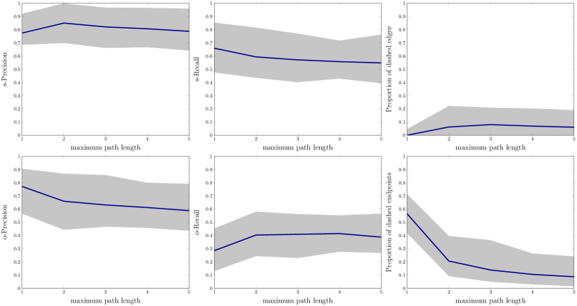
Refer to caption
Figure 10: Learning performance of COmbINE  against maximum path length. From left to right: s-Precision, s-Recall, percentage dashed edges and o-Precision, o-Recall and percentage of dashed endpoints (bottom) for varying maximum path length, averaged over all networks. Shaded area ranges from the 5 to the 95 percentile. Maximum path length 3 seems to be a be a reasonable trade-off between performance, percentage of dashed features, and efficiency.

In this section, we examine the behavior of the algorithm when the length of the paths considered is limited, in which case the output is an approximation of the actual solution. The COmbINE  pseudo-code in Algorithm 2 accepts the maximum path length as a parameter.
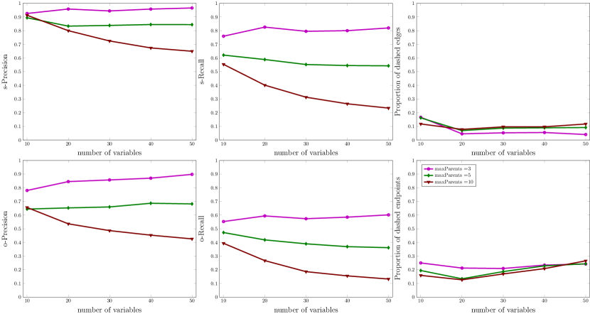
Refer to caption
Figure 11: Learning performance of COmbINE  for various network sizes and densities. From left to right: Median s-Precision, s-Recall, proportion of dashed edges (top) and o-Precision, o-Recall and proportion of dashed endpoints (bottom) for varying network size and density. Density is controlled by limiting the number of possible parents per variable. As expected, the performance deteriorates as networks become denser.

Learning performance as a function of the maximum path length is shown in Figure 10. Notice that when the path length is increased from 1 to 2 there is drop in the percentage of dashed endpoints, implying more orientations are possible. For length equal to 1, only unshielded and discriminating colliders are identified, while for length larger than 2 further orientations become possible thanks to reasoning with the inducing paths. When length is 1, notice that there are almost no dashed edges (except for the edges added in line 3 of Algorithm 3). When the maximum length increases, adjacencies in one data set, can be explained with longer inducing paths in the underlying graph and more dashed edges appear. The learning performance of the algorithm is not monotonic with the maximum length. Explaining an association (adjacency) through the presence of a long inducing path may be necessary for asymptotic correctness. However, in the presence of statistical errors, allowing such long paths could lead to complicated solutions or the propagation of errors.

Overall, it seems any increase of the maximum path length above 3 does not significantly affect performance. It seems that a maximum path length of 3 is a reasonable trade-off among learning performance (precision and recall), percentage of uncertainties, and computational efficiency. These experiments justify our choice of maximum length 3 as the default parameter value of the algorithm.

5.4 COmbINE performance as a function of network density and size

In Figure 11 the learning performance of the algorithm is presented as a function of network density and size. Density was controlled by the maximum parents allowed per variable, set by parameter maxParents during the generation of the random networks. For all network sizes, learning performance monotonically decreases with increased density, while the percentage of dashed features does not significantly vary. The size of the network has a smaller impact on the performance, particularly for the sparser networks. For dense networks, performance is relatively poor and becomes worse with larger sizes.

5.5 COmbINE performance over sample size and number of input data sets
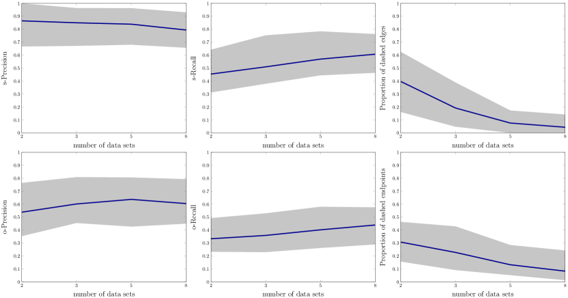
Refer to caption
Figure 12: Learning performance of COmbINE  for varying number of input data sets. From left to right: Median s-Precision, s-Recall, Proportion of dashed edges (top) and o-Precision, o-Recall and proportion of dashed endpoints of (bottom) for varying number of input data sets. Shaded area ranges from the 5 to the 95 percentile. Increasing the number of input data sets improves the performance of the algorithm.
Refer to caption
Figure 13: Learning performance of COmbINE  for varying sample size per data set. From left to right: s-Precision, s-Recall, Proportion of dashed edges (top) and o-Precision, o-Recall and proportion of dashed endpoints of (bottom) for varying sample size per data set. Shaded area ranges from the 5 to the 95 percentile. Increasing the sample size improves the performance of the algorithm.

Figure 12 shows the performance of the algorithm with increasing the number of input data sets. As expected, the percentage of uncertainties (dashed features) is steadily decreasing with increased number of input data sets. Recall also steadily improves, while Precision is relatively unaffected. Figure 13 holds the number of input data set constant to the default value 5, while increasing the sample size per data set. Recall in particular improves with larger sample sizes, while the percentage of dashed endpoints drops.

5.6 COmbINE performance for increasing number of latent variables
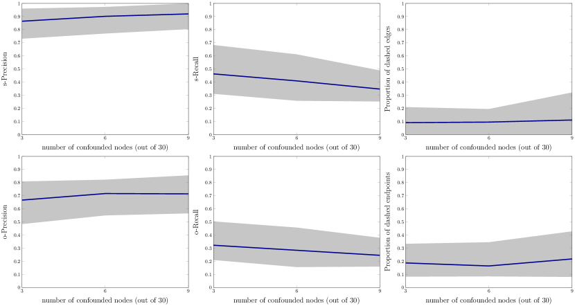
Refer to caption
Figure 14: Learning performance of COmbINE  for varying percentage of confounded variables. From left to right: s-Precision, s-Recall, percentage of dashed edges (top) and o-Precision, o-Recall and percentage of dashed endpoints (bottom) for varying number of confounded nodes for networks of 30 variables. Shaded area ranges from the 5 to the 95 percentile. Overall, the number of confounding variables does not seem to greatly affect the algorithm’ s performance.

We also examine the effect of confounding to the performance of COmbINE . To do so, we generated semi-Markov causal models instead of DAGs in the generation of the experiments: We generated random DAG networks of 30 variables and then marginalized out a percentage of the variables. Figure 14 depicts COmbINE’s performance against 3, 6, and 9 of latent variables, corresponding to 10%, 20% and 30% of the total number of variables in the graph, respectively. Overall, confounding does not seem to greatly affect the performance of COmbINE. We must point out however, that s-Recall is lower than the s-Recall with no confounded variables for the same network size (see Figure 11).

5.7 Running Time for COmbINE
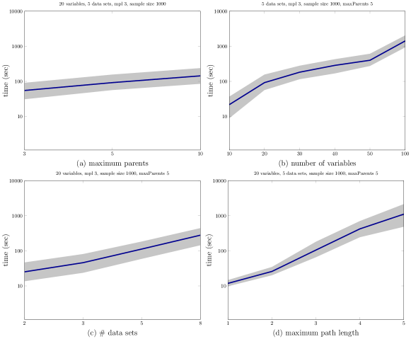
Refer to caption
Figure 15: Running time of COmbINE . From left to right: Running time (in seconds) is plotted in logarithmic scale against maximum parents per variable and number of variables (top row); number of data sets and maximum path length (bottom row). Shaded area ranges from the 5 to the 95 percentile. The number of variables and the maximum path length seem to be the most critical factors of computational performance. Notice that, COmbINE  scales up to problems with 100 total variables for limited path length and relatively sparse networks.

The running time of COmbINE  depends on several factors, including the ones examined in the previous experiments: Maximum path length, number of input data sets and sample size, and, naturally, the number of variables. Figure 15 illustrates the running time of COmbINE  against these factors. Figure 15 (b) presents the running time of COmbINE  against number of variables for networks of 5 maximum parents per variable. The experiments regarding 10 to 50 variables have also been presented in terms of learning performance in section 5.4. To further examine the scalability of the algorithm, we also ran COmbINE  in networks of 100 variables, with 5 maximum parents per variable. The experiments were ran with the default parameter values. As we can see in Figure 15, the restriction on the maximum path length is the most critical factor for the scalability of the algorithm.

5.8 A case study: Mass Cytometry data

Mass cytometry (Bendall et al., 2011) is a recently introduced technique that enables measuring protein activity in cells, and its main use is to classify hematopoietic cells and identify signaling profiles in the immune system. Therefore, the proteins are usually measured in a sample of cells and then in a different sample of the same (type of) cells after they have been stimulated with a compound that triggers some kind of signaling behavior. Identifying the causal succession of events during cell signaling is crucial to designing drugs that can trigger or suppress immune reaction. Therefore in several studies both stimulated and un-stimulated cells are treated with several perturbing compounds to monitor the potential effect on the signaling pathway.

Mass cytometry data seem to be an suitable test-bed for causal discovery methods: The proteins are measured in single cells instead of representing tissue averages, the latter being known to be problematic for causal discovery (Chu et al., 2003), and the samples range in thousands. However, the mass cytometer can measure only up to 34 variables, which may be too low a number to measure all the variables involved in a signaling pathway. Moreover, about half of these variables are surface proteins that are necessary to distinguish (gate) the cells into sub-populations, but are not functional proteins involved in the signaling pathway. It is therefore reasonable for scientists to perform experiments measuring overlapping variable sets.

Bendall et al. (2011) and Bodenmiller et al. (2012) both use mass cytometry to measure protein abundance in cells of the immune system. In both studies, the samples were treated with several different signaling stimuli. Some of the stimuli were common in both studies. After stimulation with each activating compound, Bodenmiller et al. (2012) also test the cell’s response to 27 inhibitors. One of these inhibitors is also used in Bendall et al. (2011). For this inhibitor, Bendall et al. (2011) measured bone marrow cell samples of a single donor. In Bodenmiller et al. (2012), measurements were taken from Peripheral blood mononuclear cell samples of a (different) single donor. Despite differences in the experimental setup, the signaling pathway of every stimulus and every sub-population of cells is considered universal across (healthy) donors, so the data should reflect the same underlying causal structure.

We focused on two sup-populations of the cells, CD4+ and CD8+ T-cells, which are known to play a central role in immune signaling. The data were manually gated by the researchers in the original studies. We also focused on one of the stimuli present in both studies, PMA-Ionomycin, which is known to have prominent effects on T-cells. Proteins pBtk, pStat3, pStat5, pNfkb, pS6, pp38, pErk, pZap70 and pSHP2 are measured in both data sets (initial p denotes that the concentration of the phosphorylated protein is measured). Four additional variables were included in the analysis, pAkt, pLat and pStat1 measured only in Bodenmiller et al. (2012) and pMAPK measured only in Bendall et al. (2011). To be able to detect signaling behavior, we formed data sets that contain both stimulated and unstimulated samples. As mentioned above, the cells were treated with several inhibitors. Some of these inhibitors target a specific protein, and some of them perturb the system in a more general or unidentified way. We used three target specific compounds that can be modeled as hard interventions (i.e. the compounds used to target these proteins are known to be specific and to have an effect in the phosphorylation levels of the target). More information on the specific compounds can be found in the respective publications. We ended up with four data sets for each sub-population. Details can be found in Table 3.

Data set Source latent (𝐋𝐢subscript𝐋𝐢\mathbf{L_{i}}): manipulated(𝐈𝐢subscript𝐈𝐢\mathbf{I_{i}}) Donor
𝐃𝟏subscript𝐃1\mathbf{D_{1}} Bodenmiller et al. (2012) pMAPK pAkt 1
𝐃𝟐subscript𝐃2\mathbf{D_{2}} Bodenmiller et al. (2012) pMAPK pBtk 1
𝐃𝟑subscript𝐃3\mathbf{D_{3}} Bodenmiller et al. (2012) pMAPK pErk 1
𝐃𝟒subscript𝐃4\mathbf{D_{4}} Bendall et al. (2011) pAkt, pLat, pStat1 pErk 2
Table 3: Summary of the mass cytometry data sets co-analyzed with COmbINE. The procedure was repeated for two sub-populations of cells, CD4+ cells and CD8+ cells.
Refer to caption Refer to caption
Figure 16: A case study for COmbINE: Mass cytometry data. COmbINE  was run on 4 different mass cytometry data for two different cell populations: CD4+ T-cells (left) and CD8+ T-cells (right). In each data set, one variable was manipulated (pAkt, pBTk, pErk, pErk respectively). Variables pAkt, pLat and pStat1 are only measured in data sets 1-3, while pMAPK is only measured in data set 4. Notice that pAkt is predicted to be a direct cause of pMAPK in both CD4+ and CD8+ cells, even though the two variables have never been measured together.

Protein interactions are typically non-linear, so we discretized the data into 4 bins. We ran Algorithm 2 with maximum path length 3. We used the G2superscript𝐺2G^{2} test of independence for FCI with α=0.1𝛼0.1\alpha=0.1 and maxK=5. We used Cytoscape (Smoot et al., 2011) to visualize the summary graphs produced by COmbINE, illustrated in Figure 16.

Unfortunately, the ground truth for this problem is not known for a full quantitative evaluation of the results. Nevertheless, this set of experiments demonstrates the availability of real and important data sets and problems that are suited integrative causal analysis. Second, these experiments provide a proof-of-concept for the specific algorithm. One type of interesting type of inference possible with COmbINE  and similar algorithms is the prediction that pAkt is a direct cause of pMAPK in both CD4+ and CD8+ cells, even though the variables are not jointly measured in any of the input data sets. Evidence of a direct protein interaction between the two proteins does exists in the literature Rane et al. (2001). Thus, methods for learning causal structure from multiple manipulations over overlapping variables potentially constitute a powerful tool in the field of mass cytometry.

We do not make any claims for the validity of the output graphs and they are presented only as a proof-of-concept, as there are several potential pitfalls. COmbINE  assumes lack of feedback cycles, which is not guaranteed in this system (we note however, that acyclic networks have been successfully used for reverse engineering protein pathways in the past (Sachs et al., 2005)). Causal discovery methods that allow cycles Hyttinen et al. (2013) on the other hand rely on the assumption of linearity, which is also known to be heavily violated in such networks. Thus, which set of assumptions best approximates the specific system is unknown.

6 Conclusions and Future Work

We have presented COmbINE, a sound and complete algorithm that performs causal discovery from multiple data sets that measure overlapping variable sets under different interventions in acyclic domains. COmbINE  works by converting the constraints on inducing paths in the sought out semi Markov causal model (SMCMs) that stem from the discovered (in)dependencies into a SAT instance. COmbINE  outputs a summary of the structural characteristics of the underlying SMCM, distinguishing between the characteristics that are identifiable from the data (e.g., causal relations that are postulated as present), and the ones that are not (e.g., relations that could be present or not). In the empirical evaluation the algorithm outperforms in efficiency a recently published similar one (Hyttinen et al., 2013) that, given an oracle of conditional independence, performs the same inferences by checking all m𝑚m-connections necessary for completeness.

COmbINE  is equipped with a conflict resolution technique that ranks dependencies and independencies discovered according to confidence as a function of their p-values. This technique allows it to be applicable on real data that may present conflicting constraints due to statistical errors. To the best of our knowledge, COmbINE  is the only implemented algorithm of its kind that can be applied on real data.

The algorithm is empirically evaluated in various scenarios, where it is shown to exhibit high precision and recall and reasonable behavior against sample size and number of input data sets. It scales up to networks with up to 100 variables for relatively sparse networks. Moreover, it is possible for the user to trade the number of inferences for improved computational efficiency by limiting the maximum path length considered by the algorithm. As a proof-of-concept application, we used COmbINE  to analyze a real set of experimental mass-cytometry data sets measuring overlapping variables under three different interventions.

COmbINE  outputs a summary of the characteristics of the underlying SMCM that can be identified by computing the backbone of the corresponding SAT instance. The conversion of a causal discovery problem to a SAT instance makes COmbINE  easily extendable to other inference tasks. One could instead produce all SAT solutions and obtain all the SMCMs that are plausible (i.e., fit all data sets). In this case, COmbINE  with input a single PAG would output all SMCMs that are Markov Equivalent with the PAG; there is no other known procedure for this task. Alternatively, one could easily query whether there are solution models with certain structural characteristics of interest (e.g., a directed path from A𝐴A to B𝐵B); this is easily done by imposing additional SAT clauses expressing the presence of these features. Incorporating certain types of prior knowledge such as causal precedence information can also be achieved by imposing additional path constraints. Future work includes extending this work for admitting soft interventions and known instrumental variables. The conflict resolution technique proposed could be employed to standard causal discovery algorithms that learn from single data sets, in an effort to improve their learning quality.

Appendix A.

Proof of Proposition 8
Proposition
Let 𝐎𝐎\mathbf{O} be a set of variables and 𝒥𝒥\mathcal{J} the independence model over 𝐕𝐕\mathbf{V}. Let 𝒮𝒮\mathcal{S} be a SMCM over variables 𝐕𝐕\mathbf{V} that is faithful to 𝒥𝒥\mathcal{J} and \mathcal{M} be the MAG over the same variables that is faithful to 𝒥𝒥\mathcal{J}. Let X,Y𝐎𝑋𝑌𝐎X,Y\in\mathbf{O}. Then there is an inducing path between X𝑋X and Y𝑌Y with respect to 𝐋𝐋\mathbf{L}, 𝐋𝐕𝐋𝐕\mathbf{L}\subseteq\mathbf{V} in 𝒮𝒮\mathcal{S} if and only if there is an inducing path between X𝑋X and Y𝑌Y with respect to 𝐋𝐋\mathbf{L} in \mathcal{M}.

Proof (\Rightarrow) Assume there exists a path p𝑝p in 𝒮𝒮\mathcal{S} that is inducing w.r.t. 𝐋𝐋\mathbf{L}. Then by theorem 7 there exists no 𝐙𝐕𝐋{X,Y}𝐙𝐕𝐋𝑋𝑌\mathbf{Z}\subseteq\mathbf{V}\setminus\mathbf{L}\cup\{X,Y\} such that X𝑋X and Y𝑌Y are m𝑚m-separated given 𝐙𝐙\mathbf{Z} in 𝒮𝒮\mathcal{S}, and since 𝒮𝒮\mathcal{S} and \mathcal{M} entail the same m𝑚m-separations there exists no 𝐙𝐕𝐋{X,Y}𝐙𝐕𝐋𝑋𝑌\mathbf{Z}\subseteq\mathbf{V}\setminus\mathbf{L}\cup\{X,Y\} such that X𝑋X and Y𝑌Y are m𝑚m-separated given 𝐙𝐙\mathbf{Z} in \mathcal{M}. Thus, by Theorem 6 there exists an inducing path between X𝑋X and Y𝑌Y with respect to 𝐋𝐋\mathbf{L} in \mathcal{M}.
(\Leftarrow) Similarly, assume there exists a path p𝑝p in \mathcal{M} that is inducing w.r.t. 𝐋𝐋\mathbf{L}. Then by theorem 6 there exists no 𝐙𝐕𝐋{X,Y}𝐙𝐕𝐋𝑋𝑌\mathbf{Z}\subseteq\mathbf{V}\setminus\mathbf{L}\cup\{X,Y\} such that X𝑋X and Y𝑌Y are m𝑚m-separated given 𝐙𝐙\mathbf{Z} in \mathcal{M}, and since 𝒮𝒮\mathcal{S} and \mathcal{M} entail the same m𝑚m-separations there exists no 𝐙𝐕𝐋{X,Y}𝐙𝐕𝐋𝑋𝑌\mathbf{Z}\subseteq\mathbf{V}\setminus\mathbf{L}\cup\{X,Y\} such that X𝑋X and Y𝑌Y are m𝑚m-separated given 𝐙𝐙\mathbf{Z} in 𝒮𝒮\mathcal{S}. Thus, by Theorem 7 there exists an inducing path between X𝑋X and Y𝑌Y with respect to 𝐋𝐋\mathbf{L} in 𝒮𝒮\mathcal{S}.  
Proof of Lemma 10
Lemma
Let {𝒫i}i=1Nsuperscriptsubscriptsubscript𝒫𝑖𝑖1𝑁\{\mathcal{P}_{i}\}_{i=1}^{N} be a set of PAGs and 𝒮𝒮\mathcal{S} a SMCM such that 𝒮𝒮\mathcal{S} is possibly underlying for {𝒫i}i=1Nsuperscriptsubscriptsubscript𝒫𝑖𝑖1𝑁\{\mathcal{P}_{i}\}_{i=1}^{N}, and let \mathcal{H} be the initial search graph returned by Algorithm 3 for {𝒫i}i=1Nsuperscriptsubscriptsubscript𝒫𝑖𝑖1𝑁\{\mathcal{P}_{i}\}_{i=1}^{N}. Then, if p𝑝p is an ancestral path in 𝒮𝒮\mathcal{S}, then p𝑝p is a possibly ancestral path in \mathcal{H}. Similarly, if p𝑝p is a possibly inducing path with respect to 𝐋𝐋\mathbf{L} in 𝒮𝒮\mathcal{S}, then p𝑝p is a possibly inducing path with respect to 𝐋𝐋\mathbf{L} in \mathcal{H}.

Proof  We will first prove that any path in 𝒮𝒮\mathcal{S} is a path also in \mathcal{H}, i.e. \mathcal{H} has a superset of edges compared to 𝒮𝒮\mathcal{S}. If X𝑋X and Y𝑌Y are adjacent in 𝒮𝒮\mathcal{S}, then one of the following holds:

  1. 1.

    i𝑖\exists i s.t. X,Y𝐎i𝐈i𝑋𝑌subscript𝐎𝑖subscript𝐈𝑖X,Y\in\mathbf{O}_{i}\setminus\mathbf{I}_{i}. Then the edge is present in 𝒮𝐈isuperscript𝒮subscript𝐈𝑖\mathcal{S}^{\mathbf{I}_{i}}, and X𝑋X and Y𝑌Y are adjacent in 𝒫isubscript𝒫𝑖\mathcal{P}_{i}: the edge is added to \mathcal{H} in Lines 3 of Algorithm 3.

  2. 2.

    inot-exists𝑖\not\exists i s.t. X,Y𝐎i𝐈i𝑋𝑌subscript𝐎𝑖subscript𝐈𝑖X,Y\in\mathbf{O}_{i}\setminus\mathbf{I}_{i}. Then the edge is added in \mathcal{H} in Line 3 of Algorithm 3.

Therefore, every edge in 𝒮𝒮\mathcal{S} is present also in \mathcal{H}. We must also prove that no orientation in \mathcal{H} is oriented differently in 𝒮𝒮\mathcal{S}: \mathcal{H} has only arrowhead orientations, so we must prove that, if X𝑋X Y𝑌Y in \mathcal{H} and X𝑋X and Y𝑌Y are adjacent in both graphs, X𝑋X Y𝑌Y in 𝒮𝒮\mathcal{S}.

Arrows are added to \mathcal{H} in Line 3 or in Lines 3 of the Algorithm. Arrowheads added in Line 3 occur in all 𝒫isubscript𝒫𝑖\mathcal{P}_{i}. If X Y𝑌Y in 𝒫isubscript𝒫𝑖\mathcal{P}_{i}, this means that Y𝑌Y is not an ancestor of X𝑋X in 𝒮𝐈isuperscript𝒮subscript𝐈𝑖\mathcal{S}^{\mathbf{I}_{i}}. Assume that X𝑋X Y𝑌Y in 𝒮𝒮\mathcal{S}: If X𝑋X in 𝐈isubscript𝐈𝑖\mathbf{I}_{i}, the edge would be absent in 𝒮𝐈isuperscript𝒮subscript𝐈𝑖\mathcal{S}^{\mathbf{I}_{i}} and 𝒫isubscript𝒫𝑖\mathcal{P}_{i}. If X𝐈i𝑋subscript𝐈𝑖X\not\in\mathbf{I}_{i}, X𝑋X would be ancestor of Y𝑌Y in 𝒮𝒮\mathcal{S}𝐈isubscript𝐈𝑖{}^{\mathbf{I}_{i}}, which is a contradiction. Therefore, if X𝑋X and Y𝑌Y are adjacent in 𝒮𝒮\mathcal{S}, X Y𝑌Y in 𝒮𝒮\mathcal{S}.

The latter type of arrows correspond to cases where an edge is not present in any 𝒫isubscript𝒫𝑖\mathcal{P}_{i}, inot-exists𝑖\not\exists i s.t. X,Y𝐎i𝐈i𝑋𝑌subscript𝐎𝑖subscript𝐈𝑖X,Y\in\mathbf{O}_{i}\setminus\mathbf{I}_{i}, but i𝑖\exists i s.t. X,Y𝐎i𝑋𝑌subscript𝐎𝑖X,Y\in\mathbf{O}_{i}, X𝐈i𝑋subscript𝐈𝑖X\in\mathbf{I}_{i} and Y𝐈i𝑌subscript𝐈𝑖Y\not\in\mathbf{I}_{i}. Then an arrow is added towards X𝑋X. Assume the opposite holds: X𝑋X Y𝑌Y in 𝒮𝒮\mathcal{S}, then X𝑋X Y𝑌Y in 𝒮𝐈isuperscript𝒮subscript𝐈𝑖\mathcal{S}^{\mathbf{I}_{i}}, and since both variables are observed in i𝑖i the edge would be present in 𝒫isubscript𝒫𝑖\mathcal{P}_{i}, which is a contradiction. Thus, if the edge is present in 𝒮𝒮\mathcal{S}, the edge is oriented into X𝑋X.

Thus, \mathcal{H} has a superset of edges of 𝒮𝒮\mathcal{S}, and for any edge present in both graphs, the orientations are the same. Thus, if Then, if p𝑝p is an ancestral path in 𝒮𝒮\mathcal{S}, then p𝑝p is a possibly ancestral path in \mathcal{H}. Similarly, if p𝑝p is a possibly inducing path with respect to 𝐋𝐋\mathbf{L} in 𝒮𝒮\mathcal{S}, then p𝑝p is a possibly inducing path with respect to 𝐋𝐋\mathbf{L} in \mathcal{H}.  
Proof of Lemma 11
Lemma
Let {𝐃i}i=1Nsuperscriptsubscriptsubscript𝐃𝑖𝑖1𝑁\{\mathbf{D}_{i}\}_{i=1}^{N} be a set of data sets over overlapping subsets of 𝐎𝐎\mathbf{O}, and {𝐈i}i=1Nsuperscriptsubscriptsubscript𝐈𝑖𝑖1𝑁\{\mathbf{I}_{i}\}_{i=1}^{N} be a set of (possibly empty) intervention targets such that 𝐈i𝐎isubscript𝐈𝑖subscript𝐎𝑖\mathbf{I}_{i}\subset\mathbf{O}_{i} for each i. Let 𝒫isubscript𝒫𝑖\mathcal{P}_{i} be output PAG of FCI for data set 𝐃isubscript𝐃𝑖\mathbf{D}_{i}, ΦΦsuperscript\Phi\wedge\mathcal{F}^{\prime} be the final formula of Algorithm 2, and 𝒮𝒮\mathcal{S} be a possibly underlying SMCM for {𝐏i}i=1Nsuperscriptsubscriptsubscript𝐏𝑖𝑖1𝑁\{\mathbf{P}_{i}\}_{i=1}^{N}. Then 𝒮𝒮\mathcal{S} satisfies ΦΦsuperscript\Phi\wedge\mathcal{F}^{\prime}.

Proof  Constraints in Lines 4 and 4 of Algorithm 4 are satisfied since 𝒮𝒮\mathcal{S} is a semi-Markov causal model.

Since i𝒫iisubscript𝑖subscript𝒫𝑖for-all𝑖\mathcal{M}_{i}\in\mathcal{P}_{i}\forall i, isubscript𝑖\mathcal{M}_{i} and 𝒫isubscript𝒫𝑖\mathcal{P}_{i} share the same adjacencies and non-adjacencies. If X𝑋X and Y𝑌Y are adjacent in 𝒫isubscript𝒫𝑖\mathcal{P}_{i}, X𝑋X and Y𝑌Y are adjacent in isubscript𝑖\mathcal{M}_{i}, and by Proposition 8 there exists an inducing path with respect to 𝐋isubscript𝐋𝑖\mathbf{L}_{i} in 𝒮𝐈isuperscript𝒮subscript𝐈𝑖\mathcal{S}^{\mathbf{I}_{i}}, and by Lemma 10 this path is a possibly inducing path in the initial search graph. If X𝑋X and Y𝑌Y are not adjacent in 𝒫isubscript𝒫𝑖\mathcal{P}_{i}, X𝑋X and Y𝑌Y are not adjacent in isubscript𝑖\mathcal{M}_{i}, and by Proposition 8 there exists no inducing path with respect to 𝐋isubscript𝐋𝑖\mathbf{L}_{i} in 𝒮𝐈isuperscript𝒮subscript𝐈𝑖\mathcal{S}^{\mathbf{I}_{i}}. Thus, constraints added in Line 4 of Algorithm 4 along with the corresponding literals (¬)adjacent(X,Y,𝒫i)𝑎𝑑𝑗𝑎𝑐𝑒𝑛𝑡𝑋𝑌subscript𝒫𝑖(\neg)adjacent(X,Y,\mathcal{P}_{i}) are satisfied by 𝒮𝒮\mathcal{S}.

If X𝑋X Y𝑌Y Z𝑍Z is an unshielded triple in 𝒫isubscript𝒫𝑖\mathcal{P}_{i}, X𝑋X Y𝑌Y Z𝑍Z is an unshielded triple in isubscript𝑖\mathcal{M}_{i}. If Y𝑌Y is a collider on the triple on 𝒫isubscript𝒫𝑖\mathcal{P}_{i} then Y𝑌Y is a collider on the triple on isubscript𝑖\mathcal{M}_{i} and by the semantics of edges in MAGs Y𝑌Y is not an ancestor of X𝑋X nor Z𝑍Z 𝒮𝐈isuperscript𝒮subscript𝐈𝑖\mathcal{S}^{\mathbf{I}_{i}}. Thus, constraints added to ΦΦ\Phi in Line 4 along with the corresponding literal collider(X,Y,Z,𝒫i)𝑐𝑜𝑙𝑙𝑖𝑑𝑒𝑟𝑋𝑌𝑍subscript𝒫𝑖collider(X,Y,Z,\mathcal{P}_{i}) are satisfied by 𝒮𝒮\mathcal{S}. Similarly, if Y𝑌Y is not a collider on the triple, Y𝑌Y is an ancestor of either X𝑋X or Z𝑍Z in isubscript𝑖\mathcal{M}_{i} and there exists a relative ancestral path pYXsubscript𝑝𝑌𝑋p_{YX} or pYZsubscript𝑝𝑌𝑍p_{YZ} in 𝒮𝐈isuperscript𝒮subscript𝐈𝑖\mathcal{S}^{\mathbf{I}_{i}}. By Lemma 10, this path is a possibly ancestral path in the initial \mathcal{H}. Thus, 𝒮𝒮\mathcal{S} satisfies the constraints added to ΦΦ\Phi in in Line 4 along with the corresponding literal dnc(X,Y,Z,𝒫i)𝑑𝑛𝑐𝑋𝑌𝑍subscript𝒫𝑖dnc(X,Y,Z,\mathcal{P}_{i}).

If W,,X,Y,Z𝑊𝑋𝑌𝑍\langle W,\dots,X,Y,Z\rangle is a discriminating path for V𝑉V in 𝒫isubscript𝒫𝑖\mathcal{P}_{i} and isubscript𝑖\mathcal{M}_{i} and Y𝑌Y is a collider on the path in 𝒫isubscript𝒫𝑖\mathcal{P}_{i}, then Y𝑌Y is a collider on the path in isubscript𝑖\mathcal{M}_{i}, therefore Y𝑌Y is not an ancestor of either X𝑋X or Z𝑍Z in 𝒮𝐈isuperscript𝒮subscript𝐈𝑖\mathcal{S}^{\mathbf{I}_{i}}, so 𝒮𝒮\mathcal{S} satisfies the constraints added to ΦΦ\Phi in Line 4 of Algorithm 4 along with the corresponding literal collider(X,Y,Z,𝒫i)𝑐𝑜𝑙𝑙𝑖𝑑𝑒𝑟𝑋𝑌𝑍subscript𝒫𝑖collider(X,Y,Z,\mathcal{P}_{i}). Similarly, if Y𝑌Y is not a collider on the triple, Y𝑌Y is an ancestor of either X𝑋X or Z𝑍Z in isubscript𝑖\mathcal{M}_{i} and there exists a relative ancestral path pYXsubscript𝑝𝑌𝑋p_{YX} or pYZsubscript𝑝𝑌𝑍p_{YZ} in 𝒮𝐈isuperscript𝒮subscript𝐈𝑖\mathcal{S}^{\mathbf{I}_{i}}. By Lemma 10, this path is a possibly ancestral path in the initial \mathcal{H}. Thus, 𝒮𝒮\mathcal{S} satisfies the constraints added to ΦΦ\Phi in in Line 4 along with the corresponding literal dnc(X,Y,Z,𝒫i)𝑑𝑛𝑐𝑋𝑌𝑍subscript𝒫𝑖dnc(X,Y,Z,\mathcal{P}_{i}).  
Proof of Lemma 12
Lemma
Let {𝐃i}i=1Nsuperscriptsubscriptsubscript𝐃𝑖𝑖1𝑁\{\mathbf{D}_{i}\}_{i=1}^{N}, {𝐈i}i=1Nsuperscriptsubscriptsubscript𝐈𝑖𝑖1𝑁\{\mathbf{I}_{i}\}_{i=1}^{N}, {𝐏i}i=1Nsuperscriptsubscriptsubscript𝐏𝑖𝑖1𝑁\{\mathbf{P}_{i}\}_{i=1}^{N}, ΦΦsuperscript\Phi\wedge\mathcal{F}^{\prime} be defined as in Lemma 11. If graph S satisfies ΦΦsuperscript\Phi\wedge\mathcal{F}^{\prime}, then 𝒮𝒮\mathcal{S} is a possibly underlying SMCM for {𝐏i}i=1Nsuperscriptsubscriptsubscript𝐏𝑖𝑖1𝑁\{\mathbf{P}_{i}\}_{i=1}^{N}.

Proof 𝒮𝒮\mathcal{S} is a SMCM: 𝒮𝒮\mathcal{S} is by construction a mixed graph, and it satisfies constraints in Lines 4 and 4 of Algorithm 4, so it has no directed cycles, and at most one tail per edge.

isubscript𝑖\mathcal{M}_{i} and 𝒫isubscript𝒫𝑖\mathcal{P}_{i} share the same edges: If X𝑋X and Y𝑌Y are adjacent in 𝒫isubscript𝒫𝑖\mathcal{P}_{i}, then by the constraints in Line 4 of Algorithm 4 there exists an inducing path with respect to 𝐋isubscript𝐋𝑖\mathbf{L}_{i} in 𝒮𝐈isuperscript𝒮subscript𝐈𝑖\mathcal{S}^{\mathbf{I}_{i}}, therefore X𝑋X and Y𝑌Y are adjacent in isubscript𝑖\mathcal{M}_{i}. If X𝑋X and Y𝑌Y are not adjacent in 𝒫isubscript𝒫𝑖\mathcal{P}_{i} then by the same constraints there exists no inducing path with respect to 𝐋isubscript𝐋𝑖\mathbf{L}_{i} in 𝒮𝐈isuperscript𝒮subscript𝐈𝑖\mathcal{S}^{\mathbf{I}_{i}}, therefore X𝑋X and Y𝑌Y are not adjacent in isubscript𝑖\mathcal{M}_{i}.

isubscript𝑖\mathcal{M}_{i} and 𝒫isubscript𝒫𝑖\mathcal{P}_{i} share the same unshielded colliders: Let X𝑋X Y𝑌Y Z𝑍Z be an unshielded triple in 𝒫isubscript𝒫𝑖\mathcal{P}_{i}. Since 𝒫isubscript𝒫𝑖\mathcal{P}_{i} and isubscript𝑖\mathcal{M}_{i} share the same edges, X𝑋X Y𝑌Y Z𝑍Z is an unshielded triple in isubscript𝑖\mathcal{M}_{i}. If the triple is an unshielded collider in 𝒫isubscript𝒫𝑖\mathcal{P}_{i} then by the constraints in Line 4 of Algorithm 4 Y𝑌Y is not an ancestor of either X𝑋X or Z𝑍Z in 𝒮𝐈isuperscript𝒮subscript𝐈𝑖\mathcal{S}^{\mathbf{I}_{i}}, thus X𝑋X Y𝑌Y Z𝑍Z in isubscript𝑖\mathcal{M}_{i}. If on the other hand the triple is a definite non-collider in 𝒫isubscript𝒫𝑖\mathcal{P}_{i}, then by the constraints in Line 4 of Algorithm 4 Y𝑌Y is an ancestor of either X𝑋X or Z𝑍Z in 𝒮𝐈isuperscript𝒮subscript𝐈𝑖\mathcal{S}^{\mathbf{I}_{i}}, therefore either Y𝑌Y X𝑋X or Y𝑌Y Z𝑍Z in isubscript𝑖\mathcal{M}_{i}, thus, the triple is an unshielded non-collider in isubscript𝑖\mathcal{M}_{i}.

If W,,X,Y,Z𝑊𝑋𝑌𝑍\langle W,\dots,X,Y,Z\rangle is a discriminating path for V𝑉V in both isubscript𝑖\mathcal{M}_{i} and 𝒫isubscript𝒫𝑖\mathcal{P}_{i}, and Y𝑌Y is a collider on the path, then by the constraints in Line 4 of Algorithm 4 Y𝑌Y is not an ancestor of X𝑋X or Z𝑍Z in 𝒮𝐈isuperscript𝒮subscript𝐈𝑖\mathcal{S}^{\mathbf{I}_{i}}, therefore Y𝑌Y is a collider on the same path in isubscript𝑖\mathcal{M}_{i}. If, conversely, Y𝑌Y is not a collider on the path, then by the constraints in Line 4 of Algorithm 4, Y𝑌Y is an ancestor of either X𝑋X or Z𝑍Z, thus, X𝑋X is not a collider on the same path in isubscript𝑖\mathcal{M}_{i}.  

References

  • Beinlich et al. (1989) IA Beinlich, HJ Suermondt, RM Chavez, and GF Cooper. The ALARM monitoring system: A case study with two probabilistic inference techniques for belief networks. In Second European Conference on Artificial Intelligence in Medicine, volume 38, pages 247–256. Springer-Verlag, Berlin, 1989.
  • Bendall et al. (2011) SC Bendall, EF Simonds, P Qiu, El-ad D Amir, PO Krutzik, R Finck, RV Bruggner, R Melamed, A Trejo, OI Ornatsky, RS Balderas, SK Plevritis, K Sachs, D Peér, SD Tanner, and GP Nolan. Single-cell mass cytometry of differential immune and drug responses across a human hematopoietic continuum. Science, 332(6030):687–696, 2011.
  • Bodenmiller et al. (2012) B Bodenmiller, ER Zunder, R Finck, TJ Chen, ES Savig, RV Bruggner, EF Simonds, SC Bendall, K Sachs, PO Krutzik, et al. Multiplexed mass cytometry profiling of cellular states perturbed by small-molecule regulators. Nature biotechnology, 30(9):858–867, 2012.
  • Borboudakis et al. (2012) G Borboudakis, S Triantafillou, and I Tsamardinos. Tools and algorithms for causally interpreting directed edges in maximal ancestral graphs. In Sixth European Workshop on Probabilistic Graphical Models(PGM), 2012.
  • Chu et al. (2003) T Chu, C Glymour, R Scheines, and P Spirtes. A statistical problem for inference to regulatory structure from associations of gene expression measurements with microarrays. Bioinformatics, 19(9):1147–1152, 2003.
  • Claassen and Heskes (2010a) T Claassen and T Heskes. Causal discovery in multiple models from different experiments. In Advances in Neural Information Processing Systems (NIPS 2010), volume 23, pages 1–9, 2010a.
  • Claassen and Heskes (2010b) T Claassen and T Heskes. Learning causal network structure from multiple (in) dependence models. In Proc. of the Fifth European Workshop on Probabilistic Graphical Models (PGM), pages 81–88, 2010b.
  • Claassen and Heskes (2012) T Claassen and T Heskes. A Bayesian Approach to Constraint Based Causal Inference. In Proceedings of the 28th Conference on Uncertainty in Artificial Intelligence (UAI2012), pages 207–217, 2012.
  • Colombo et al. (2012) Diego Colombo, Marloes H. Maathuis, Markus Kalisch, and Thomas S. Richardson. Learning high-dimensional directed acyclic graphs with latent and selection variables. The Annals of Statistics, 40(1):294–321, 02 2012.
  • Cooper and Yoo (1999) GF Cooper and Ch Yoo. Causal discovery from a mixture of experimental and observational data. In Proceedings of Uncertainty in Artificial Intelligence (UAI 1999), volume 10, pages 116–125, 1999.
  • Eaton and Murphy (2007a) D Eaton and K Murphy. Belief net structure learning from uncertain interventions. J Mach Learn Res, 1:1–48, 2007a.
  • Eaton and Murphy (2007b) D Eaton and K Murphy. Bdagl: Bayesian dag learning. http://www.cs.ubc.ca/ murphyk/Software/BDAGL/, 2007b.
  • Eberhardt and Scheines (2007) F Eberhardt and R Scheines. Interventions and causal inference. Philosophy of science, 74(5):981–995, 2007.
  • Eén and Sörensson (2004) N Eén and N Sörensson. An extensible SAT-solver. In Theory and Applications of Satisfiability Testing, pages 333–336, 2004.
  • Evans and Richardson (2010) RJ Evans and TS Richardson. Maximum likelihood fitting of acyclic directed mixed graphs to binary data. In Proceedings of the 26th International Conference on Uncertainty in Artificial Intelligence, 2010.
  • Evans and Richardson (2011) RJ Evans and TS Richardson. Marginal log-linear parameters for graphical markov models. arXiv preprint arXiv:1105.6075, 2011.
  • Fisher (1922) RA Fisher. On the interpretation of χ𝜒\chi2 from contingency tables, and the calculation of p. Journal of the Royal Statistical Society, 85(1):87–94, 1922.
  • Geiger and Heckerman (1994) Dan Geiger and David Heckerman. Learning gaussian networks. In Proceedings of the Tenth Conference Annual Conference on Uncertainty in Artificial Intelligence (UAI-94), pages 235–243, San Francisco, CA, 1994. Morgan Kaufmann.
  • Gomes et al. (2000) Carla P Gomes, Bart Selman, Nuno Crato, and Henry Kautz. Heavy-tailed phenomena in satisfiability and constraint satisfaction problems. Journal of automated reasoning, 24(1-2):67–100, 2000.
  • Hauser and Bühlmann (2012) A Hauser and P Bühlmann. Characterization and Greedy Learning of Interventional Markov Equivalence Classes of Directed Acyclic Graphs. JMLR, 13, August 2012.
  • Hyttinen et al. (2012a) A Hyttinen, F Eberhardt, and PO Hoyer. Learning linear cyclic causal models with latent variables. JMLR, 13:3387–3439, 2012a.
  • Hyttinen et al. (2012b) A Hyttinen, F Eberhardt, and PO Hoyer. Causal discovery of linear cyclic models from multiple experimental data sets with overlapping variables. In Uncertainty in Artificial Intelligence, 2012b.
  • Hyttinen et al. (2013) A Hyttinen, PO Hoyer, F Eberhardt, and M Järvisalo. Discovering cyclic causal models with latent variables: A general sat-based procedure. In Uncertainty in Artificial Intelligence, 2013.
  • Kuegel (2010) Adrian Kuegel. Improved exact solver for the weighted max-sat problem. In Workshop Pragmatics of SAT, 2010.
  • Meganck et al. (2006) S Meganck, S Maes, P Leray, and B Manderick. Learning semi-markovian causal models using experiments. In Third European Workshop on Probabilistic Graphical Models(PGM), 2006.
  • Murphy (2001) K Murphy. Active learning of causal bayes net structure. Technical report, UC Berkeley, 2001.
  • Ramsey et al. (2006) J Ramsey, P Spirtes, and J Zhang. Adjacency faithfulness and conservative causal inference. In Proceedings of Uncertainty in Artificial Intelligence, 2006.
  • Rane et al. (2001) MJ Rane, PY Coxon, DW Powell, R Webster, JB Klein, W Pierce, P Ping, and KR McLeish. p38 kinase-dependent mapkapk-2 activation functions as 3-phosphoinositide-dependent kinase-2 for akt in human neutrophils. Journal of Biological Chemistry, 276(5):3517–3523, 2001.
  • Richardson and Spirtes (2002) TS Richardson and P Spirtes. Ancestral graph markov models. The Annals of Statistics, 30(4):962–1030, 2002.
  • Richardson et al. (2012) TS Richardson, JM Robins, and I Shpitser. Nested markov properties for acyclic directed mixed graphs. In Proceedings of the Twenty Eighth Conference on Uncertainty in Artificial Intelligence, page 13. AUAI Press, 2012.
  • Sachs et al. (2005) K Sachs, O Perez, D Pe’er, DA Lauffenburger, and GP Nolan. Causal protein-signaling networks derived from multiparameter single-cell data. Science, 308(5721):523–529, 2005.
  • Sellke et al. (2001) T Sellke, MJ Bayarri, and JO Berger. Calibration of ρ𝜌\rho values for testing precise null hypotheses. The American Statistician, 55(1):62–71, 2001.
  • Shpitser et al. (2013) I Shpitser, R Evans, TS Richardson, and JM Robins. Sparse nested markov models with log-linear parameters. In Proceedings of the Twenty Ninth Conference on Uncertainty in Artificial Intelligence (UAI-13), pages 576–585. AUAI Press, 2013.
  • Smoot et al. (2011) ME Smoot, K Ono, J Ruscheinski, PL Wang, and T Ideker. Cytoscape 2.8: new features for data integration and network visualization. Bioinformatics, 27(3):431–432, 2011.
  • Spirtes and Richardson (1996) P Spirtes and TS Richardson. A polynomial time algorithm for determining DAG equivalence in the presence of latent variables and selection bias. In Proceedings of the 6th International Workshop on Artificial Intelligence and Statistics, pages 489–500, 1996.
  • Spirtes et al. (2001) P Spirtes, C Glymour, and R Scheines. Causation, Prediction, and Search. The MIT Press, second edition, January 2001.
  • Storey and Tibshirani (2003) JD Storey and R Tibshirani. Statistical significance for genomewide studies. Proceedings of the National Academy of Sciences of the United States of America, 100(16):9440, 2003.
  • Tian and Pearl (2003) J Tian and J Pearl. On the identification of causal effects. Technical Report R-290-L, UCLA Cognitive Systems Laboratory, 2003.
  • Tillman and Spirtes (2011) RE Tillman and P Spirtes. Learning equivalence classes of acyclic models with latent and selection variables from multiple datasets with overlapping variables. In Proceedings of the 14th International Conference on Artificial Intelligence and Statistics, volume 15, pages 3–15, 2011.
  • Tillman et al. (2008) RE Tillman, D Danks, and C Glymour. Integrating locally learned causal structures with overlapping variables. In Advances in Neural Information Processing Systems (NIPS, 2008.
  • Tong and Koller (2001) S Tong and D Koller. Active learning for structure in bayesian networks. In International joint conference on artificial intelligence, pages 863–869, 2001.
  • Triantafillou et al. (2010) S Triantafillou, I Tsamardinos, and IG Tollis. Learning causal structure from overlapping variable sets. In Proceedings of Artificial Intelligence and Statistics, volume 9, 2010.
  • Tsamardinos et al. (2012) Ioannis Tsamardinos, Sofia Triantafillou, and Vincenzo Lagani. Towards integrative causal analysis of heterogeneous data sets and studies. The Journal of Machine Learning Research, 98888:1097–1157, 2012.
  • Verma and Pearl (2003) TS Verma and J Pearl. Equivalence and Synthesis of Causal Models. Technical Report R-150, UCLA Department of Computer Science, 2003.
  • Zhang (2006) J Zhang. Causal inference and reasoning in causally insufficient systems. PhD thesis, PhD thesis, Carnegie Mellon University, 2006.
  • Zhang (2008a) J Zhang. On the completeness of orientation rules for causal discovery in the presence of latent confounders and selection bias. Artificial Intelligence, 172(16-17):1873–1896, 2008a.
  • Zhang (2008b) J Zhang. Causal Reasoning with Ancestral Graphs. Journal of Machine Learning Research, 9(1):1437–1474, 2008b.