Adjoint accuracy for the full-Stokes ice flow model: limits to the transmission of basal friction variability to the surface

Zusammenfassung

This work focuses on the numerical assessment of the accuracy of an adjoint-based gradient in the perspective of variational data assimilation and parameter identification in glaciology. Using noisy synthetic data, we quantify the ability to identify the friction coefficient for such methods with a non-linear friction law. The exact adjoint problem is solved, based on second order numerical schemes, and a comparison with the so called “self-adjoint” approximation, neglecting the viscosity dependency to the velocity (leading to an incorrect gradient), common in glaciology, is carried out. For data with a noise of $1\%$, a lower bound of identifiable wavelengths of $10$ ice thicknesses in the friction coefficient is established, when using the exact adjoint method, while the “self-adjoint” method is limited, even for lower noise, to a minimum of $20$ ice thicknesses wavelengths. The second order exact gradient method therefore provides robustness and reliability for the parameter identification process. In other respect, the derivation of the adjoint model using algorithmic differentiation leads to formulate a generalization of the “self-adjoint” approximation towards an incomplete adjoint method, adjustable in precision and computational burden.

The main available observations of the cryosphere are generally obtained from remote-sensed techniques and are thus essentially surface observations. However, ice dynamics is known to be highly sensitive to the state of the bed (and therefore to how the bed is modeled, see e.g. Cuffey and Paterson (2010)), not to the surface which is more easily observable. The friction coefficient is consequently a critical parameter in terms of controlling ice flows. This raises questions about, on one hand, whether the surface can provide the necessary information about basal conditions and, on the other hand, whether inverse methods can adequately recover this information.

Many authors have address the first question by investigatin how bedrock topography affects the surface. Balise and Raymond (1985) conducted one of the earliest studies concerning the transmission of fluctuations in basal slip to the surface for a Newtonian fluid, using perturbation methods. The non-local aspect of the transmission of the variations of the friction coefficient at surface is established by Raymond (1996) where it is dependent upon the slip ratio (ratio between mean sliding velocities and mean ice deformation velocities). These queries are extended in Gudmundsson (2003), still under the Newtonian hypothesis using perturbation methods. In these studies, one of the main conclusions is that the transmission of basal variability at the surface increases with increased sliding.

The question of the representability of the friction coefficient through surface velocity observations (horizontal and vertical) using an inverse method is studied by Gudmundsson and Raymond (2008). The method, based on a Bayesian approach, is used to study the effect of density and quality of surface velocity data on the estimation of the friction coefficient for a Newtonian fluid and a linear sliding law. In the reconstruction of small amplitude variations of the friction coefficient, a wavelength limit of around $50$ times the ice thickness is found. A similar method in the case of a non-Newtonian fluid and a non-linear sliding law is developed in Raymond and Gudmundsson (2009).

In other respects, the identification method based on MacAyeal (1993) and widely used (see e.g. Larour et al. (2005); Joughin et al. (2004); Morlighem et al. (2010)) makes the assumption that viscosity is independent of the velocity, and a limited attention has been paid to the quality of the resulting estimations in terms of spatial variability of the friction coefficient (see Gudmundsson and Raymond (2008)). Comparisons with the “self-adjoint” method and the use of an exact adjoint are made by Goldberg and Sergienko (2011), based on a vertically integrated approximation and by Morlighem et al. (2013) based on the higher-order model. Limitations for the minimizing process are highlighted by Goldberg and Sergienko (2011) when using the “self-adjoint” method. To the best of our knowledge, the use of an exact adjoint in a glaciological context for the full-Stokes problem has been done only by Petra et al. (2012). A comparison between their results and the results of Gudmundsson and Raymond (2008) on an academic problem allowed then to conclude that the exact adjoint is able to recover wavelengths in the friction coefficient of approximately $20$ times the ice thickness in the case of a linear sliding law.

The purpose of this study is the numerical evaluation of the limitations of the “self-adjoint” method compared to the method using the exact adjoint solution, referred as the full adjoint method in what hereafter. The “self-adjoint” approximation for the full-Stokes problem is detailed in terms of equations and presented as a limited case of the reverse accumulation method used to compute the adjoint when obtained using source-to-source automatic differentiation. From a strictly numerical perspective, tests on the accuracy reached by the gradients for both methods are performed, demonstrating an important limitation for the gradient computed by the “self-adjoint” method. We then study the identifiability, for a non-linear sliding law, of high frequencies in the friction coefficient depending on the level of noise considered on synthetic data. The quality of the estimations provided by both methods is compared in the case of dense horizontal surface velocity observations for a quasi-uniform flow and then for a realistic flow presenting an important spatial variability. The realistic case is then applied for less dense data.

1 Forward and adjoint model

In this section, we briefly present what shall be referred to hereafter as the forward model and describe the derivation of the adjoint model and the computation of the adjoint state.

1.1 Forward model

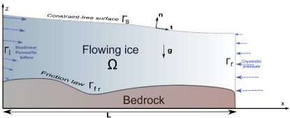
The flow model considered here is the bidimensional flowline power-law Stokes model applied to a gravity driven flow (see e.g. Cuffey and Paterson (2010)) and solved on a given domain $\Omega$ of horizontal extent $L$ (see Figure 1):

$$\hskip 72.26999pt\mathbf{div}(\mathbf{u})= 0 \leavevmode\nobreak\ \mbox{ in }\Omega,$$ (1)

$$-\mathbf{div}(2\eta(\mathbf{u})\underline{\boldsymbol{D}})+\nabla p= \rho\mathbf{g} \leavevmode\nobreak\ \mbox{ in }\Omega,$$ (2)

$$\eta(\mathbf{u})=\eta_{0}\|\underline{\boldsymbol{D}}\|_{F}^{\frac{1-n}{n}}.$$ (3)

where $\underline{\boldsymbol{\sigma}}=\eta(\mathbf{u})\underline{\boldsymbol{D}}-p\boldsymbol{Id}$ represents the Cauchy stress tensor (with $\boldsymbol{Id}$ the second-order two-dimension identity tensor), $\eta(\mathbf{u})$ the viscosity, $\eta_{0}$ the consistency of the fluid, $n$ the power-law exponent, $\underline{\boldsymbol{D}}$ the strain rate tensor, $\mathbf{u}=(u_{x},u_{z})$ the velocity field defined in the Cartesian frame $(x,z)$, $p$ the pressure field, $\rho$ the ice density, $\mathbf{g}$ the gravity and $\|\underline{\boldsymbol{D}}\|^{2}_{F}=\underline{\boldsymbol{D}}:\underline{\boldsymbol{D}}$ the Frobenius matrix norm.

A Weertman-type sliding law is then prescribed at the bedrock boundary $\Gamma_{fr}$:

$$|\mathbf{\sigma}_{nt}|^{m-1}\mathbf{\sigma}_{\mathbf{n}\mathbf{t}}= \beta\mathbf{u}\cdot\mathbf{t} \mbox{ on }\Gamma_{fr},$$ (4)

$$\mathbf{u}\cdot\mathbf{n}= 0 \leavevmode\nobreak\ \mbox{ on }\Gamma_{fr}.$$ (5)

where $\beta=\beta(x)$ is a spatially variable parameter and where $(\boldsymbol{t},\boldsymbol{n})$, the tangent-normal pair of unit vectors, is such that:

$$\underline{\boldsymbol{\sigma}}=(\underline{\boldsymbol{\sigma}}\cdot\boldsymbol{n})\boldsymbol{n}+(\underline{\boldsymbol{\sigma}}\cdot\boldsymbol{t})\boldsymbol{t}\quad$$ (6)

and:

$$\underline{\boldsymbol{\sigma}}\cdot\boldsymbol{n}=\sigma_{nn}\boldsymbol{n}+\sigma_{nt}\boldsymbol{t}\quad,\quad\underline{\boldsymbol{\sigma}}\cdot\boldsymbol{t}=\sigma_{tn}\boldsymbol{n}+\sigma_{tt}\boldsymbol{t}$$ (7)

A velocity profile corresponding to the solution of the Stokes problem for a uniform steady flow of a parallel sided slab on an inclined bed with non-linear friction defined by (4) at the bottom is prescribed on the inflow boundary. This solution $\mathbf{u}=(u_{\overline{x}},u_{\overline{z}})$, expressed in the “mean-slope” reference frame $(\overline{x},\overline{z})$, is written (see e.g. Martin (2013)):

$$\begin{array}[]{c}u_{\overline{x}}(\overline{z})=\displaystyle{\frac{(-\rho\mathbf{g}sin(\theta)h)^{m}}{\beta}}+\\ \displaystyle{\frac{1}{1+n}(2\eta_{0})^{-n}(\rho\mathbf{g}sin(\theta))^{n}(h^{1+n}-(H-\overline{z})^{1+n})},\\ \end{array}$$ (8)

$${u_{\overline{z}}=0},$$ (9)

$${p(\overline{z})=\rho gcos(\theta)(H-\overline{z})}.$$ (10)

with $\theta$ defining the slope of the slab, $H$ the height of the upper-surface and $h$ the thickness.

A hydrostatic pressure is considered on the outflow. All the simulations are performed with an exponent $m=3$ for the sliding law. The domain is discretized using triangular Taylor-Hood finite elements and the solution of the continuous forward problem is obtained using a classical fixed point algorithm. The geometry and notations of the problem are plotted in Figure 1.

Abbildung 1: Geometry, boundary conditions and notations of the problem

The sensitivities and identifications carried out in this work use adjoint-based computation and thus require the solution of the adjoint problem associated with the full-Stokes model.

All the computations are performed using the software DassFlow (DassFlow Software (2007)). The fixed point algorithm is used here as a typical iterative method for solving of the full-Stokes problem but the assessments on the precision and efficiency of the adjoint-based inverse problems should be valid for any iterative algorithm. The details on the different approaches used in DassFlow for the solution of the power-law Stokes problem can be found in Martin and Monnier (2014a).

1.2 The basic principles of the adjoint model

The output of the forward model is represented by a scalar valued function $j$ called a cost function, which depends on the parameters of the model and represents a quantity to be minimized. In presence of observations, part of the cost measures the discrepancy (the misfit) between the computed state and an observed state (through any type of data).

The parameters of interest are called control variables and constitute a control vector $\boldsymbol{k}$. The minimizing procedure operates on this control vector to generate a set of parameters which allows a computed state closer to the observations to be obtained. In the following the control vector includes only the friction coefficient field $\beta(x)$. The corresponding optimal control problem can be written:

$$\underset{\boldsymbol{k}}{Min}\hskip 3.99994ptj(\boldsymbol{k})$$ (11)

This optimization problem is solved numerically by a descent algorithm. Thus, we need to compute the gradient of the cost function. This is done by introducing the adjoint model.

1.3 Cost Function, Twin Experiments and Morozov’s Discrepancy Principle

The cost function used for the identification is defined by:

$$j(\beta;\gamma)=\frac{1}{2}\int_{\Gamma_{s}}\|u^{obs}_{s}(\beta_{t})-u_{s}(\beta)\|_{2}^{2}\leavevmode\nobreak\ \leavevmode\nobreak\ d\mathbf{x}+\gamma\mathcal{T}(\beta^{\prime}),$$ (12)

where the data $u^{obs}_{s}$ are synthetic horizontal surface velocities obtained using a given friction coefficient $\beta_{t}$ and perturbed with a random Gaussian noise of varying level $\delta$. The term $\mathcal{T}(\beta^{\prime})$ called Tikhonov’s regularization controls the oscillations of the control variable gradient $\beta^{\prime}$. It is defined by:

$$\mathcal{T}(\beta^{\prime})=\int_{[0,L]}\|\beta^{\prime}\|^{2}_{2}\leavevmode\nobreak\ ds.$$ (13)

where $L$ is the length of the domain. The parameter $\gamma$ quantifies the strength of the imposed smoothness. This term regularizes the functional to be minimized and introduces a bias toward smoothly varying field. The tuning of these weights can be achieved from various considerations generally related to the quality of the data (or the noise level) and the degree of smoothness sought on the control variable. A classical approach, referred to as the Morozov’s discrepancy principle (see e.g. Vogel (2002)), consists of choosing $\gamma$ such that $j(\beta;\gamma)=j(\beta_{t};0)$ i.e. when the final cost matches the noise level on the data. The methodology that consists of using noisy synthetic data in order to retrieve a set of reference parameters (here defined as $\beta_{t}$) a priori known is called a twin experiment. The gradient of the cost function is given by solving the adjoint problem and used by the algorithm to compute at each iteration a new set of parameters in order to make the cost $j$ decrease until convergence.

1.4 Derivation of the adjoint model

In order to efficiently compute all partial derivatives of a cost function $j(\boldsymbol{k})$ with respect to the components of a control vector $\boldsymbol{k}$, we introduce the adjoint model (see e.g. Lions, J.L. (1971)).

In DassFlow software, the adjoint model is obtained by using algorithmic differentiation of the source code (see Honnorat (2007); Honnorat et al. (2007); DassFlow Software (2007)). This last approach ensures a better consistency between the computed cost function and its gradient, since it is the computed cost function that is differentiated. A large part of this extensive task can be automated using automatic differentiation (see Griewank et al. (1989)). In the case of DassFlow-Ice, the direct code is written in Fortran 95 and is derived using the automatic differentiation tool Tapenade (see Hascoët and Pascual (2004)). The linear solver used is MUMPS (Amestoy et al. (2001)) and the differentiation of the linear system solving process is achieved using a “bypass” approach which considers the linear solver as an unknown black-box (see appendix A). This approach is similar to the one used by Goldberg and Heimbach (2013).

Let $\mathcal{K}$ be the space of control variables and $\mathcal{Y}$ the space of the forward code response. In the present case, we have :

$$\boldsymbol{k}=(\beta)\mbox{ and }Y=(y,j)^{T}$$

where $\beta$ is defined by (4).

Let us point out that we include both the state and the cost function in the response of the forward code. The direct code can be represented as an operator $\mathcal{M}\,:\mathcal{K}\longrightarrow\mathcal{Y}$ such that:

$$\mathcal{Y}=\mathcal{M}(\mathcal{K}).$$

The tangent model becomes $\frac{\partial\mathcal{M}}{\partial\boldsymbol{k}}(\boldsymbol{k})\,:\mathcal{K}\longrightarrow\mathcal{Y}$. As input variable, it takes a perturbation of the control vector $d\boldsymbol{k}\in\mathcal{K}$, it then gives the variation $dY\in\mathcal{Y}$ as output variable:

$$dY=\frac{\partial\mathcal{M}}{\partial\boldsymbol{k}}(\boldsymbol{k})\cdot d\boldsymbol{k}\ .$$

The adjoint model is defined as the adjoint operator of the tangent model. This can be represented as follows:

$$\left(\frac{\partial\mathcal{M}}{\partial\boldsymbol{k}}(\boldsymbol{k})\right)^{*}\,:\mathcal{Y}^{\prime}\longrightarrow\mathcal{K}^{\prime}.$$

It takes $dY^{*}\in\mathcal{Y}^{\prime}$ as an input variable and provides the adjoint variable $d\boldsymbol{k}^{*}\in\mathcal{K}^{\prime}$ at output:

$$d\boldsymbol{k}^{*}=\left(\frac{\partial\mathcal{M}}{\partial\boldsymbol{k}}(\boldsymbol{k})\right)^{*}\!\!\cdot dY^{*}\ .$$

Now, let us make the link between the adjoint code and the gradient $\frac{dj}{d\boldsymbol{k}}$ we seek to compute. By definition of the adjoint, we have :

$$\textstyle\Big{\langle}\left(\frac{\partial\mathcal{M}}{\partial\boldsymbol{k}}\right)^{*}\!\!\cdot dY^{*},\,d\boldsymbol{k}\Big{\rangle}_{\mathcal{K}^{\prime}\times\mathcal{K}}=\ \Big{\langle}dY^{*},\,\left(\frac{\partial\mathcal{M}}{\partial\boldsymbol{k}}\right)\cdot d\boldsymbol{k}\Big{\rangle}_{\mathcal{Y}^{\prime}\times\mathcal{Y}}\ .$$ (14)

It reads, using the relations presented above:

$$\textstyle\big{\langle}d\boldsymbol{k}^{*},\,d\boldsymbol{k}\big{\rangle}_{\mathcal{K}^{\prime}\times\mathcal{K}}=\ \big{\langle}dY^{*},\,dY\big{\rangle}_{\mathcal{Y}^{\prime}\times\mathcal{Y}}\ .$$ (15)

If we set $dY^{*}=(0,1)^{T}$ and by denoting the perturbation vector $d\boldsymbol{k}=\left(\delta\beta\right)^{T}$, we obtain:

$$\begin{array}[]{lcr}&\textstyle\left\langle\left(\begin{array}[]{c}0\\ 1\end{array}\right),\,\left(\begin{array}[]{c}dy^{*}\\ dj^{*}\end{array}\right)\right\rangle_{\mathcal{Y}^{\prime}\times\mathcal{Y}}\par&=\ \Bigg{\langle}\left(\begin{array}[]{c}\delta\beta^{*}\end{array}\right),\left(\begin{array}[]{c}\delta\beta\end{array}\right)\Bigg{\rangle}_{\mathcal{K}^{\prime}\times\mathcal{K}}.\\ \end{array}$$

Furthermore, we have by definition:

$$dj\ =\ \frac{\partial j}{\partial\beta}(\boldsymbol{k})\cdot\delta\beta.$$ (16)

Therefore, the adjoint variable $d\boldsymbol{k}^{*}$ (output of the adjoint code with $dY^{*}=(0,1)^{T}$) corresponds to the partial derivatives of the cost function $j$:

$$\frac{\partial j}{\partial\beta}(\boldsymbol{k})=\beta^{*}.$$ (17)

A single integration of the forward model followed by a single integration of the adjoint model allow to compute all components of the gradient of the cost function.

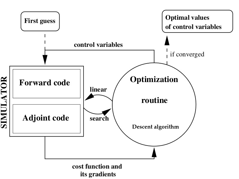
The optimal control problem (11) is solved using a local descent algorithm, more precisely the L-BFGS algorithm (a quasi-Newton method), implemented in the M1QN3 routine (see Gilbert and Lemaréchal (1989)). Thus, these partial derivatives are used as input to the minimization algorithm M1QN3. The global optimization process is represented in Figure 2.

Abbildung 2: Principle of a 3D-Var type variational data assimilation algorithm.

1.5 The gradient test

The gradient test is a classical adjoint code validation test and is used hereafter in order to assess the precision of the “self-adjoint” approximation. The test aims to verify that the partial derivatives of the cost function are correctly computed by comparing it with a finite difference approximation (see e.g. Honnorat et al. (2007) for the detailed test procedures).

Let us consider the following order two central finite difference approximation of the gradient:

$$\frac{j(\mathbf{k}+\alpha\delta\mathbf{k})-j(\mathbf{k}-\alpha\delta\mathbf{k})}{2\alpha}=\frac{\partial j}{\partial\mathbf{k}}\cdot\delta\mathbf{k}+O\left(\alpha^{2}\delta\mathbf{k}^{3}\right)$$ (18)

with $d\boldsymbol{k}=\alpha\delta\boldsymbol{k}$. This scheme leads us to define:

$$I_{\alpha}\ =\ \frac{j(\mathbf{k}+\alpha\,\delta\mathbf{k})-j(\mathbf{k}-\alpha\,\delta\mathbf{k})}{2\alpha\;\frac{\partial j}{\partial\mathbf{k}}(\mathbf{k})\cdot\delta\mathbf{k}}\ .$$ (19)

According to (18), one must have: $\displaystyle\lim_{\alpha\rightarrow 0}\>I_{\alpha}=1$.
The gradient test consists of verifying this property.

2 “Self-adjoint” approximation, full adjoint and reverse accumulation

The model considered here has been obtained using algorithmic (or automatic) differentiation of the source code. Automatic differentiation of a fixed point type iterative routine of the form $y=\Phi(y,u)$ (such as the solution of the non-linear Stokes problem using a Picard method) is carried out by reverse accumulation (see Griewank et al. (1989, 1993)). The reverse accumulation technique consists of building a computational graph for the function evaluation where the nodes of the graph represent every value taken by the function. To every node, an adjoint quantity containing the gradient of the function $\Phi$ with respect to the node, is associated.

The adjoint values are computed in reverse order. The final value of the gradient is given by the sum of the partial derivatives of the function of the nodes of the computational graph. This result is a consequence of the chain rule. This process a priori requires the storing of as many states of the system as iterations performed by the forward solver to reach the converged state.

It is shown by Christianson (1994) that, in the case of a forward computation carried out by a fixed point method, the adjoint quantity also satisfies a fixed point problem whose rate of convergence is at least equal to the rate of convergence of the forward fixed point. Based on this result, it is a priori necessary to retain every iteration of the forward run to evaluate the gradient. In practice, as further detailed in section 2.4, the number of reverse iterations required to obtain an adjoint state with the same precision of the forward state can be adjusted depending on the convergence speed of the direct construction.

2.1 The “self-adjoint” approximation

The “self-adjoint” method in glaciology, applied to the shelfy-stream approximation, has been proposed by MacAyeal (1993). The approximation consists of deriving the adjoint equation system without taking into account the explicit dependency of the viscosity $\eta$ on the velocity field $\mathbf{u}$. Let us recall that the terminology self-adjoint only makes sense in the Newtonian case ($n=1$). It is important to precise that the gradient resulting from this procedure is therefore an incorrect gradient.

For the full-Stokes case, the adjoint system considered under this approximation is the adjoint associated to the forward problem (1)-(2) using a viscosity field $\eta(u_{0})=2\eta_{0}\|\underline{\boldsymbol{D}}(u_{0})\|_{F}$ for a given $u_{0}$. This problem is indeed a “self-adjoint” problem (the underlying operator is linear and symmetrical with respect to $\mathbf{u}$).

In general, the procedure consists of calculating a mechanical equilibrium based on the complete non-linear system to obtain a converged $u_{0}$ and the gradient is then obtained by simply transposing the final computed state. This method applied to the full-Stokes problem can be found in Morlighem et al. (2010).

In the automatic differentiation context, this approximation is equivalent to retain, in the reverse accumulation process, only the gradient computed from the final evaluation of the function $\Phi$. The quality of such an approximation is thus questionable and will strongly depend on the problem one considers and the required accuracy on the gradient.

The quality of this approximation (compared to the exact adjoint state) for parameter identification is assessed by Goldberg and Sergienko (2011) for depth-integrated shallow-ice type equations but has never been treated for the full-Stokes equations.

2.2 The continuous adjoint system

Before the numerical assessment of the “self-adjoint” approximation it seems relevant to look into the continuous adjoint equation system in order to highlight the terms that are being ignored by the approximation and to estimate their weight in the complete adjoint system.

Omitting the lateral boundaries, the adjoint system of the full-Stokes problem (1)-(5) is (see e.g. Petra et al. (2012)):

$$-\operatorname{\boldsymbol{div}}(\underline{\boldsymbol{\Sigma}}) = 0\mbox{ in }\Omega,$$ (20)

$$\operatorname{\boldsymbol{div}}(\mathbf{v}) = 0\mbox{ in }\Omega,$$ (21)

$$\underline{\boldsymbol{\Sigma}}\boldsymbol{n} = \mathbf{u}_{s}^{obs}-\mathbf{u}\mbox{ on }\Gamma_{s},$$ (22)

$$\Sigma_{nt} = \beta^{1/m}\left(|\mathbf{u}_{\tau}|^{\frac{1-m}{m}}\mathbf{v}_{\tau}+\right.,$$ (23)

$$\left.(m-1)|\mathbf{u}_{\tau}|^{\frac{1-3m}{m}}(\mathbf{u}_{\tau}\otimes\mathbf{u}_{\tau})\mathbf{v}_{\tau}\right)\mbox{ on }\Gamma_{fr},$$

$$\mathbf{v}\cdot\boldsymbol{n} = 0\mbox{ on }\Gamma_{fr},$$ (24)

where $\mathbf{v}$ denotes the adjoint velocity and $\underline{\boldsymbol{\Sigma}}$ the adjoint stress tensor. The quantity $\Sigma_{nt}$ is defined in the same way as $\sigma_{nt}$ (see equation (7)). The adjoint stress tensor is written:

$$\underline{\boldsymbol{\Sigma}}=2\eta(\mathbf{u})\left(\textrm{I}+\frac{2(1-n)}{n}\frac{\underline{\boldsymbol{D}}(\mathbf{u})\otimes\underline{\boldsymbol{D}}(\mathbf{u})}{\|\underline{\boldsymbol{D}}(\mathbf{u})\|_{F}^{2}}\right)\underline{\boldsymbol{D}}(\mathbf{v})-\operatorname{\boldsymbol{Id}}q$$ (25)

with $q$ denoting the adjoint pressure, I the fourth-order identity tensor applied to order two tensors, $\operatorname{\boldsymbol{Id}}$ the second order identity tensor and ${}^{\prime}\otimes^{\prime}$ the tensor product.

By construction, this problem is a linear problem in $\mathbf{v}$ and depends on the forward velocity $\mathbf{u}$. The method to derive the adjoint system associated to any non-linear elliptic problem can be found in e.g. Monnier (2013).

First, the non-linearity of the forward problem appears in the definition of the adjoint stress given in equation (25). The norm of the term $\frac{\underline{\boldsymbol{D}}(\mathbf{u})\otimes\underline{\boldsymbol{D}}(\mathbf{u})}{\|\underline{\boldsymbol{D}}(\mathbf{u})\|_{F}^{2}}$ is simply one (since $\|\underline{\boldsymbol{D}}\otimes\underline{\boldsymbol{D}}\|=\|\underline{\boldsymbol{D}}\|_{F}\times\|\underline{\boldsymbol{D}}\|_{F}$ given a consistent choice of the fourth-order tensor norm with the Frobenius matrix norm) and the norm of the identity tensor is known to be greater or equal to one (and typically equal to one for the sup norm). The linearity assumption of the ßelf-adjointmethod leads to set $n=m=1$ in the adjoint system (20)-(24). It then leads to the dropping of a term that is comparable to the one that is kept, for $\frac{1-n}{n}$ close to one ($2/3$ for $n=3$). It logically follows that the greater the non-linearity (the value of $n$), the greater the non-linear contribution, and the coarser the “self-adjoint”approximation.

The other non-linearity comes from the non-linear friction law and appears in equation (23). A similar calculation leads to a similar conclusion: for $m>1$, the norm of the terms that are being dropped by the “self-adjoint” approximation is comparable to the one being kept.

Let us point out that, in equation (23), for larger values of $m$ (representing hard-rock sliding or mimicking Coulomb friction), the nonlinear contribution is no longer comparable to the linear part and becomes dominant due to the factor $(m-1)$, and to neglect the nonlinear terms is most certainly unsuited.

These observations are clearly retrieved numerically in the gradient test performed hereafter (see Figure 3) which shows a relative error around $1$ for the “ self-adjoint” approximation.

2.3 Numerical evaluation of the “self-adjoint” approximation

We consider the flow described in section 1.1. The domain is a parallel sided slab on an inclined bed with an aspect ratio of $1/10$ on a $10\%$ slope. The friction condition at the bottom is given by (4) with a constant $\beta$ and an exponent $m=3$. A stationary free surface flow, uniform with respect to $x$, is thus obtained.

The cost function $j$ used here corresponds to the one defined by (12) withtout regularization:

$$j=j(\beta;0)=\frac{1}{2}\int_{\Gamma_{s}}\left|u(\beta,\overline{z})-u_{s}^{obs}\right|^{2}\leavevmode\nobreak\ d\overline{\boldsymbol{x}}$$ (26)

where the observations $u^{obs}$ are the horizontal velocities at the surface $\Gamma_{s}$, $(\overline{x},\overline{z})$ designates the mean-slope frame and the control variable is the discrete friction coefficient field $\beta$.

Abbildung 3: Gradient test for the full adjoint method the “self-adjoint” method for various levels of precision $\nu$ of the forward solution. The quantity $I_{\alpha}$ is defined by (19).

The gradient tests carried out for the “self-adjoint” and full adjoint methods, using cost function (26), are plotted in Figure 3. The tests are performed for various levels of precision of the forward problem $\nu=\|u_{k+1}-u_{k}\|/\|u_{k}\|$ in order to quantify the best attainable precision by the adjoint problem with respect to $\nu$. This precision is explicitly given to the direct solver through a convergence threshold for the nonlinear loop but can be seen as the available accuracy on the data $u^{obs}$ ; a direct solution accuracy $\nu=10^{-4}$ mimics data presenting a noise of $0.01\%$. The use of unnoisy data helps to preserve the theoretical constant rate decreasing error of the gradient test, thus validating the method.

The gradient test compares the gradient computed by the adjoint code to a reference gradient. For these tests, the reference gradient is obtained using a centered finite difference approximation (of order $2$) computed for a precision on the function evaluation of $10^{-12}$. This precision being considerably higher than those considered for the solution of the forward problem, the finite difference gradient plays the role of an “exact” value (see section 1.5).

The full adjoint method shows the expected theoretical behavior. We recover the slope of $2$ (in logarithmic scale) associated with the order of convergence of the finite difference approximation (18). Figure 3 thus shows that the precision of the adjoint state is of the same order as the one of the direct solver.

On the contrary, the precision of the gradient provided by the “self-adjoint” approximation is rather limited. The best reachable precision, as expected from the continuous adjoint system analysis, is slightly smaller than $1$ irrespective of the direct solver precision $\nu$ (and thus, only one gradient test curve is plotted in Figure 3, for the case $\nu=10^{-8}$, $\nu$ being the precision of the forward solution).

The “self-adjoint” approximation used within a parameter identification process is thus not able to compute an accurate gradient. However, as further discussed thereafter, numerical tests demonstrate a certain ability for this approximation to partially reconstruct the friction coefficient (for a computational cost well below the one of the full adjoint method in the automatic differentiation context). Nevertheless, significant weaknesses for the reconstruction of high frequencies as well as the reconstruction of the main frequency of the friction coefficient signal, specifically for extreme situations of sliding (very slow or very fast), are brought to the forefront.

2.4 Adjustable adjoint accuracy & truncation of the reverse accumulation

This section focuses on the effect of a truncation of the reverse accumulation process. Figure 4 plots gradient test results obtained for a truncated evaluation of the adjoint state. To do so, the number of iterations of the adjoint loop is truncated from one to $N$, the total number of iterations performed by the direct solver. We thus obtain $N$ gradient tests providing every level of precision for each intermediary adjoint states between the exact adjoint ($N$ iterations) and the “self-adjoint” approximation. This test is carried out for various levels of precision $\nu$ of the direct solver. The number of iterations $N$ performed by the direct solver to reach the required accuracy $\nu$ depends on this precision.

Abbildung 4: Accuracy of the gradient for incomplete reverse accumulation for various levels of precision of the direct solution $\nu$.

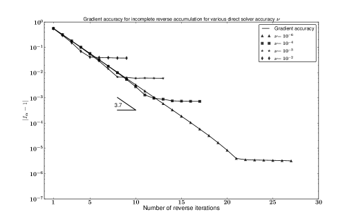
The results concerning the precision of the gradient presented previously are well recovered (see Figure 3). The lowest precision, identical for every $\nu$ and equal to $0.6$, is obtained from the “self-adjoint” approximation (corresponding to $1$ reverse iteration) and the highest precision is reached by the full adjoint method (corresponding to the last point of each curve).

A linear decrease of the error (in logarithmic scale) resulting in a slope of $3.7$ is observed. This behavior of the error is coherent with the result of Christianson (1994) who states that the computation of the adjoint state by reverse accumulation is equivalent to a fixed point computation. In the present case, we have a reverse accumulation algorithm presenting a rate of convergence of $3.7$. Yet, the convergence speed of the forward fixed point (not plotted here) leads to a slope of $3$. The convergence of the adjoint state computation is therefore higher than the one of the direct state computation. This result explains the plateau observed for the final iterations; indeed, a faster convergence of the reverse accumulation algorithm allows us to reach the converged adjoint state with fewer iterations.

Again, the accuracy of the “self-adjoint” approximation appears strongly limited and the possibility of an incomplete method, intermediary between the full adjoint method and the retention of only one iteration could bring an important gain of precision ; taking into account the linearly decreasing error (in logarithmic scale) leads to significantly improved accuracy for each additional iteration retained during the computation of the adjoint state.

Furthermore, the faster convergence of the reverse accumulation algorithm compared to the direct solver allows, in any case, to spare a few iterations during the computation of the adjoint state without any loss of precision. The number of unnecessary iterations is likely to be strongly dependent on the situation and must be studied in every case.

For the present test case, we observe that the $5$ last iterations during the reverse accumulation are useless whatever the level of precision of the forward run (see the plateau in Figure 4). These $5$ last iterations correspond to the $5$ first iterations carried out by the direct solver. Avoiding the accumulation of these iterations for the adjoint state evaluation amounts to starting the reverse accumulation from a residual on the forward run of $0.1$ (i.e. a relative variation between two successive iterates of $0.1$). This observation, although dependent on the considered case, can be seen as an empirical method to define a criteria on the number of direct iterations that should be accumulated to obtain the best accuracy on the adjoint state. In the present case, it amounts to initiating the memory storage of direct iterations once the direct solver residual is lower than $0.1$.

In a more general point of view, the threshold imposed on the direct solver to limit the accuracy of the computed state is a quite numerical artifice and should not be seen as a way of saving time, regardless of the data precision. A reliable approach for real numerical simulations could be to perform an accurate direct simulation but a truncated adjoint in adequation with the level of noise on the data. This adjustment could be made based on one gradient test which allows to quantify the rate of convergence of the reverse accumulation loop.

3 Friction coefficient identifiability

This section focuses on the practical limits of identifiability of the friction coefficient by both the full adjoint and the “self-adjoint” method.

The main goal is to draw conclusions on the possibility of using the “self-adjoint” method (which brings an important time and memory saving) and then on the quality of the results it provides in the perspective of realistic identification of the friction coefficient. The quality of the results is evaluated in terms of frequencies and amplitudes of the reconstructed friction coefficients compared to the target ones.

As presented before, the precision of the “self-adjoint” gradient is bounded, whatever the level of precision of the direct solver $\nu$. This level of precision can be seen as an a priori accuracy on the data considered in the cost function. In view of a thorouh analysis of the invertibility capacities of an adjoint-based inverse method, only synthetic data are used in the present work. A Gaussian noise of level $\delta$ is thus added a posteriori to emulate real data. The precision of the exact adjoint gradient depending on $\nu$ (and equivalently on the level of noise $\delta$ on the data), we seek to observe which value of $\nu$ is required to observe the limit of precision of the self-adjoint method.

To this end, we consider three noise levels $\delta$ of $0.01\%$, $0.1\%$ and $1\%$. representing referred as very low, low and realistic noise. Although, a realistic level of noise depends on many aspects, the use of GPS techniques and InSAR velocity measurements can provide this type of precision (King (2004), Joughin et al. (2010), Rignot et al. (2011)).

In all cases, the final cost reached by both methods is not sufficient enough to inform their precision, especially for noise level greater or equal to 1% (which is typically the case for real data). This means that one cannot draw conclusions about the quality of the “self-adjoint” approximation solely based on a comparison of the costs provided by both methods.

On the contrary the frequency analysis suggests that an identical final cost is not equivalent to an identical inferred friction coefficient. It demonstrates that this type of inverse problem is ill-posed, which can be seen as an equifinality issue (i.e. an identical state, and consequently an identical cost, can be obtained with different sets of input parameters).

It is important to point out that the poorer the data (or similarly the greater the noise), the stronger the equifinality.

In what follows, we first consider the idealized case of a quasi-uniform flow on an inclined parallel sided slab with very low and low noise level in order to highlight the numerical limits of the “self-adjoint” method.

We then perform pseudo-realistic, spatially variable, flow experiments with a realistic noise for various density of the surface data. All the identifications presented hereafter use, as an initial guess for the friction coefficient, the average value $a$ of the target coefficient. The optimization procedure stops when the three following criterions are achieved: a relative variation of the cost smaller than $10^{-8}$, a relative variation of the norm of the gradient smaller than $10^{-4}$ and a relative variation of the norm of the inferred friction coefficient smaller than $10^{-4}$.

3.1 Quasi-uniform flow

The following experiments are performed on the same inclined parallel sided slab as in section 2.3. A non-linear friction law, defined by (4) is considered at the bottom with an exponent $m=3$. The target friction coefficient, variable in $x$, is given by:

$$\beta_{r}^{N}(x)=a+\frac{a}{2}\sin\left(\frac{2\pi x}{20dx}\right)+\frac{a}{5}\sum_{i=1}^{N}f_{i}(x)$$ (27)

with

$$f_{i}(x)=\sin\left(\frac{2\pi x}{w_{i}dx}\right)\mbox{ with }w_{1}=10,\leavevmode\nobreak\ w_{2}=4,\leavevmode\nobreak\ w_{3}=2,$$ (28)

and by extension, we set:

$$\boldsymbol{f_{0}}(x)=\sin\left(\frac{2\pi x}{w_{0}dx}\right)\mbox{ with }w_{0}=20.$$ (29)

The quantity $a$ is the average value of the friction coefficient in $\mbox{Pa}\cdot\mbox{s}\cdot\mbox{m}^{-1}$ and $dx=0.2$m denotes the length of a basal edge or, in other words, the sharpness of the bedrock discretization.

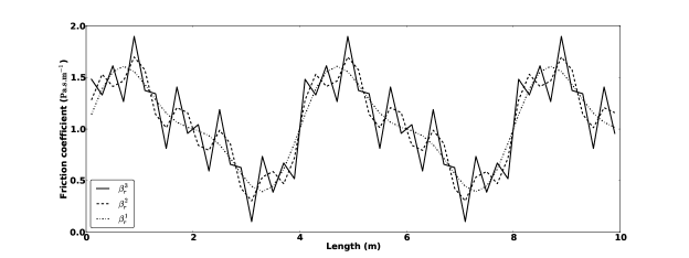
We set $\beta_{r}=\beta_{r}^{3}$, the friction coefficient resulting from the sum of $4$ frequencies corresponding to wavelengths of $20$, $10$, $5$ and $2$ edge length $dx$. The low frequency $f_{0}$ represents a carrier wave for the $3$ higher frequencies $f_{i},i\in\llbracket 1,3\rrbracket$. In terms of thickness of the domain $h$ (here constant and equal to $1$m, see Table 1), frequencies $f_{i},i\in\llbracket 1,3\rrbracket$ correspond to wavelengths of $4h$, $2h$, $0.8h$ and $0.4h$ respectively. The coefficients $\beta_{r}^{N},N\in\llbracket 1,3\rrbracket$ are plotted in Figure 5 for the case $a=1$. These properties are summarized in Table 1.

Abbildung 5: Friction coefficient $\beta_{r}^{n},1\leq n\leq 3$ given by (27) with $a=1$.

	$\boldsymbol{f_{0}}$	$f_{1}$	$f_{2}$	$f_{3}$
Wavelength w.r.t $h=1$m (thickness)	$4h$	$2h$	$0.8h$	$0.4h$
Wavelength w.r.t. $dx=0.2$m (edge length)	$20dx$	$10dx$	$4dx$	$2dx$
Wavenumber w.r.t. $L=10$m (domain length)	$2.5$m-1	$5$m-1	$12.5$m-1	$25$m-1

Tabelle 1: Characteristics of signal $\beta$ given by (27).

The flow is uniform when the friction coefficient is constant along the domain and can be described as quasi-uniform when the friction coefficient is given by (27).

We seek to determine the level of spatial variability of the friction coefficient the full adjoint and the “self-adjoint” methods can provide through the identification process, based on surface velocity observations, with respect to the degree of slip. The degree of slip depends on the value of parameter $a$ and will be described thereafter in terms of slip ratio $r$. The slip ratio is a dimensionless quantity that quantifies how slippery the bedrock is. It is calculated as the ratio of the mean sliding velocity $\overline{u_{b}}$ to the difference between mean surface velocity$\overline{u_{s}}$ and mean basal velocity $\overline{u_{b}}$ (cf. Hindmarsh (2004)). It leads to:

$$r=\overline{u_{b}}/|\overline{u_{s}}-\overline{u_{b}}|.$$ (30)

A slip ratio $r=1$ represents a situation where half of the surface velocities are attributed to sliding and half are attributed to deformation.

We consider $6$ different slip ratios ranging from very high friction (close to adherence) to very rapid sliding. The slip ratios $r=0.005$, $r=0.05$ and $r=0.5$ can be described as moderate sliding and the slip ratios $r=5$, $r=50$ and $r=500$ as rapid sliding.

In order to highlight the limitations of the “self-adjoint” approximation, the identifications of $\beta$ performed hereafter consider noise levels $\delta=0.1\%$ and $\delta=0.01\%$ on the surface velocity data. Let us point out that the “self-adjoint” method provides very similar results to the full adjoint one in terms of final cost when $\delta=1\%$ (not plotted in Figure 6) and the distinction between both methods clearly appears for lower noises.

The cost function is defined by (12). The tuning of the regularization parameter $\gamma$ is achieved according to the Morozov discrepancy principle (see section 1.3). We plot in Figure 6 the application of this method to the identifications performed with both methods (full adjoint and “self-adjoint”) in the case of an intermediate friction ($r=0.5$). The corresponding curves for other slip ratios are identical and consequently not plotted.

Abbildung 6: Application of Morozov’s discrepancy principle. Final discrepancy (or misfit) $j_{1}=\int_{\Gamma_{s}}\left|u_{s}(n)-u_{s}^{obs}(n_{t})\right|^{2}\leavevmode\nobreak\ d\boldsymbol{x}$ with respect to the value of the regularization parameter $\gamma$. The horizontal line represents the level of noise corresponding to the optimal discrepancy obtained from the target coefficient.

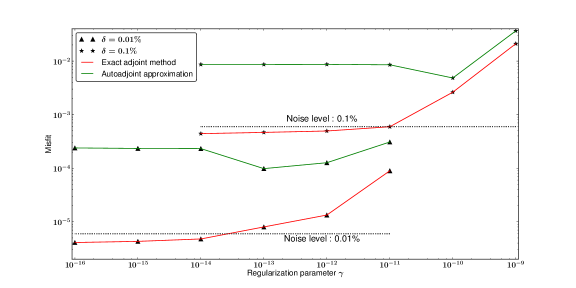
Figure 6 clearly demonstrates the inability, for the “self-adjoint” method, to provide a gradient for sufficiently low noise. For noise levels $\delta=0.1\%$ and $\delta=0.01\%$, the “self-adjoint” gradient does not allow the optimal misfit to be reached. Therefore, in these situations, the “self-adjoint” approximation is theoretically not valid. However, as we will see, the “self-adjoint” method shows a certain ability to retrieve the target parameter. This observation is independent of the degree of slip.

In order to study the effects of the approximation on the gradient computation, we compare, in the following, the friction coefficient inferred by both methods for $\delta=0.01\%$ and $\delta=0.1\%$.

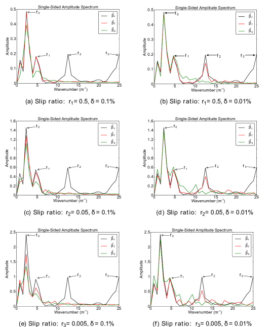
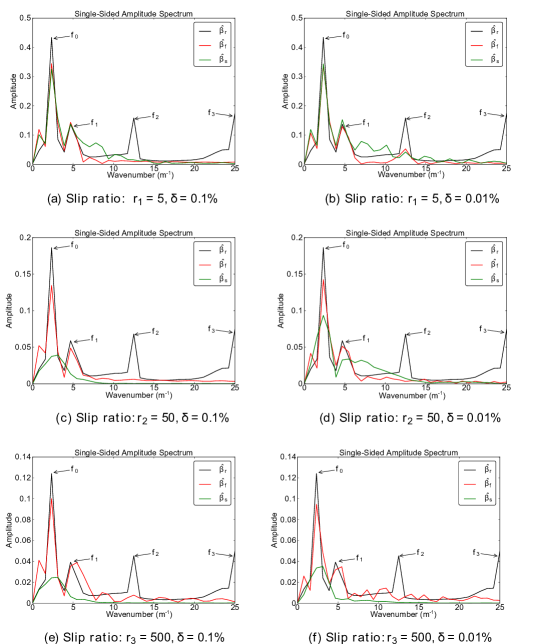
The best inferred friction coefficient (according to Morozov) are noted $\beta_{f}$ for the full-adjoint and $\beta_{s}$ for the self-adjoint. The quantities $\widehat{\beta_{f}}$ and $\widehat{\beta_{s}}$ thus denote their associated Discrete Fourier Transform (DFT). We denote by $\widehat{\beta_{r}}$ the DFT associated to the target friction coefficient (27). The single-sided amplitude spectrum of the DFTs $\widehat{\beta_{r}}$, $\widehat{\beta_{f}}$ and $\widehat{\beta_{s}}$ obtained for the three small slip ratios (moderate sliding) are plotted in Figure 7 and those obtained for the three high slip ratios (rapid sliding) are plotted in Figure 8. The amplitude spectrum plots the modulus of the complex Fourier coefficient multiply by two, providing the original amplitude of the frequencies of the signal (approximated by the sharpness of the sampling frequency). The abscissae have been rescaled according to the discretization of the bedrock $dx$ and the length of the domain $L$ in order to directly provide the original wavenumber of the frequencies. All the signals have been centered (to have a zero mean) in order to remove the peak corresponding to the average. Since the zero mean amplitude spectrum is symmetrical, the single-sided spectrum is plotted everywhere. The single-sided amplitude spectrum plotted in Figures 12, and 14 are identically defined.

Abbildung 7: Discrete Fourier Transform of inferred friction coefficient $\beta_{f}$ and $\beta_{s}$ and of the target friction coefficient $\beta_{r}$. Moderate sliding.

Abbildung 8: Discrete Fourier Transform of inferred friction coefficient $\beta_{f}$ and $\beta_{s}$ and of the target friction coefficient $\beta_{r}$. Rapid sliding.

Moderate sliding

One observes first that frequencies $f_{0}$ and $f_{1}$ (see Table 1) are globally well reproduced by both methods for $\delta=0.01\%$ whatever the slip ratio. Namely the carrier frequency $f_{0}$ is very well reconstructed by both methods and this property seems desirable. The full adjoint method shows a greater robustness when identifying these two low frequencies with respect to the slip ratio whereas a noticeable deterioration for the identification of frequency $f_{1}$ occurs for the “self-adjoint” method when slip ratio decreases.

However, frequency $f_{2}$ appears correctly captured by the full adjoint method while it does not appear in the spectrum of the “self-adjoint” one. An increased difficulty in capturing this frequency occurs with slip ratio increasing.

Finally, the highest frequency $f_{3}$ does not appear in any of the spectrums of both $\beta_{f}$ and $\beta_{s}$ whatever the degree of slip.

For a noise level $\delta=0.1\%$, one loses the ability to retrieve frequency $f_{2}$ using the full adjoint method. The identification of frequency $f_{1}$ is accurately obtained for the slip ratio $r_{1}=0.5$ but we observe a deterioration of the result when slip ratio decreases. The “self-adjoint” method captures almost none of frequency $f_{1}$ whatever the slip ratio.

Concerning the carrier frequency, one observes difficulties for the “self-adjoint” method to reconstruct it accurately even for the slip ratio $r_{1}=0.5$. The frequency distinctly appears on the spectrum but only $80\%$ of the target amplitude is recovered. The decreasing of the slip ratio deteriorates, for both methods, the identification of $f_{0}$. In the case $r_{3}=0.005$, the full adjoint method recovers $70\%$ of the target amplitude where the “self-adjoint” method recovers $50\%$.

Rapid sliding

Again, low frequencies $f_{0}$ and $f_{1}$ are well retrieved with the full adjoint method for every noise level. The carrier wave reconstruction is nevertheless diminished (around $80\%$ of the target amplitude) compared to the moderate sliding situation $r_{1}=0.5$ but is stable with the increasing of $r$. Similarly, frequency $f_{1}$ is rather well represented by the full adjoint method for all the situations despite a certain degradation with increasing $r$. However, frequency $f_{2}$ does not appear in any spectrum irrespective of both slip ratio and method, contrarily to the moderate sliding situations. Again, frequency $f_{3}$ is never captured. A small but noticeable noise appears for the case $r=500$ for the full adjoint method, particularly when $\delta=0.01\%$.

The “self-adjoint” method shows a relatively good reconstruction of $f_{0}$ and $f_{1}$ for the case $r=5$ but introduces noise between frequencies $f_{1}$ and $f_{2}$. A strong deterioration of the reconstruction occurs when $r$ increases ; for a noise level $\delta=0.1\%$, the “self-adjoint” identification is almost unable to recover the signal for $r\geq 50$.

Assessments

From these observations, we draw the following conclusions. Firstly, the degree of slip of the target plays a strong role for the limit of identifiability of the friction coefficient in terms of frequencies ; a smaller slip ratio induces a lower sensitivity of the flow to the friction coefficient and consequently a higher filtering on the transmission of information from the bedrock to the surface.

A strong friction induces a vertical velocity profile that is rather convex with velocity gradients (shearing) mostly concentrated close to the bottom leading to a weaker transmission of the information from the bottom to the surface. A similar observation can be made from the sensitivity of the model to the rheological constant $\eta_{0}$: the high sensitivity areas are strongly correlated to the areas of high shearing.

Similar to strong frictions, low frictions also reduce the quality of the reconstruction. This again comes from a reduced sensitivity of the flow to the friction coefficient when rapid sliding occurs however this lower sensitivity appears for different reasons. Intuitively, the case of a very low friction leads to lower local topographical effects and the resistance to the ice flow acts through an equivalent global topography at larger scale. This characteristic appears in the explicit solution of the uniform flow (8): in order for the mathematical expression to make sense when $\beta$ tends to $0$, it requires the slope parameter $\theta$ to tend to $0$ as well. This phenomena is physically observed: in the presence of an extended sub-glacial lake, one observes a signature of this lake at the surface as a very flat surface topography over the lake. This interpretation is retrieved in the normalized sensitivities plotted in Figure 13.

These two observations support the existence of a numerical identifiability maximum for the friction coefficient using adjoint-based method ; the best situation to carry out identifications corresponds to the intermediate friction range where sliding effects and deformation effects on the dynamics are balanced (typically $0.5<r<5$). The low accuracy of the “self-adjoint” gradient appears to be a strong limitation in the case of rapid sliding ($r>5$).

For the current quasi-uniform flow, for a noise level $\delta=0.1\%$, a limit on identifiable wavelength using the full adjoint method, for any degree of slip, is $2h$, where $h$ is the thickness of the domain. More accurate data could allow us to infer higher frequencies in the case of moderate sliding ($r\geq 0.5$).

For the “self-adjoint” method, for a slip ratio $r\leq 5$, a wavelength of $4h$ is well inferred and a wavelength of $2h$ is captured for $r=0.5$ and $r=5$. For a slip ratio $r>5$, the frequencies considered in the experiment are inappropriate.

In other respects, a tendency for the “self-adjoint” method to introduce non-physical interferences within the inferred coefficient for very low noise appears. This non desirable phenomena increases when the slip ratio takes on extreme values. Beyond the approximation aspect, one can deduce a lack of robustness of the “self-adjoint” method for very low noises. It seems coherent with regards to the low precision the “self-adjoint” gradient provides. On the contrary, the full adjoint method provides a less accurate identification when the slip ratio goes away from $1$ without introducing non physical effects in the inferred parameter.

It is of interest to notice that the inability to recover frequency $f_{3}$ is not a numerical limitation but a limitation due to the noise on the data. For sufficiently accurate data, it is also identifiable using the second order exact adjoint method.

Similar experiments are performed in the next section for a pseudo-realistic flow ran on a radar vertical profile of the grounded part of the Mertz glacier in Antarctica for surface velocity data with different density and a $1\%$ noise.

3.2 Real topography flow: the Mertz glacier

The flow considered in this section is identical to the one presented in subsection 1.1. The computational domain is built from real field data; topography of the bedrock and of the surface are bidimensional radar-sensed layers of the Mertz ice tongue in East Antarctica. These layers have been measured along a flowline of this outlet glacier (American program ICECAP 2010, see Greenbaum et al. (2010)). Our study focuses on the grounded part of the glacier. The computational domain is plotted in Figure 9.

Abbildung 9: Vertical cut of the outlet glacier Mertz, Antarctica (topography profile from ICECAP 2010 within Ice bridge, provided by B. Legrésy, LEGOS, France) , x-scale $=2/5$

Synthetic data are obtained using the following friction coefficient:

$$\beta_{r}^{N}(x)=a+\frac{a}{2}\sin\left(\frac{2\pi x}{50dx}\right)+\frac{a}{5}\sum_{i=1}^{N}f_{i}(x)$$ (31)

with

$$f_{i}(x)=\sin\left(\frac{2\pi x}{w_{i}dx}\right)\mbox{ with }w_{1}=20,\leavevmode\nobreak\ w_{2}=10,\leavevmode\nobreak\ w_{3}=5,$$ (32)

and by extension, we set:

$$\boldsymbol{f_{0}}(x)=\sin\left(\frac{2\pi x}{w_{0}dx}\right)\mbox{ with }w_{0}=50.$$ (33)

The quantity $a$ is the average friction coefficient and $dx=100$m is the bedrock edge length. The context of a non-uniform flow on a complex topography allows to carry on the comparison between both methods in the case of a realistic flow simulation. We can then draw practical conclusions on the validity of using the “self-adjoint” approximation. Frequency $f_{0}$ is a carrier wave with $50dx$ wavelength corresponding to $5h$, where $h\sim 1$km is the average thickness of the domain. Frequencies $f_{1}$, $f_{2}$ and $f_{3}$ correspond then to wavelengths of $2h$, $h$ and $h/2$ respectively, providing a situation similar to the inclined slab test case (see Table 2).

	$\boldsymbol{f_{0}}$	$f_{1}$	$f_{2}$	$f_{3}$
Wavelength w.r.t $h=1$km (thickness)	$5h$	$2h$	$h$	$0.5h$
Wavelength w.r.t $dx=100$m (edge length)	$50dx$	$20dx$	$10dx$	$5dx$
Wavenumber w.r.t $L=33.3$km (domain length)	$6.6$m-1	$16.6$m-1	$33.3$m-1	$66.6$m-1

Tabelle 2: Characteristics of signal $\beta$ given by (31).

In the present case of a non uniform flow with complex topography, it is not feasible to simulate an average slip ratio $r=500$. Given the important spatial variability, we are able to achieve a maximum average slip ratio $r=50$. In the following identification, we consider only $5$ slip ratios ranging from $r=0.005$ to $r=50$. The synthetic horizontal surface velocity perturbed with a $1\%$ noise are plotted in Figure10 for the case $r=5$.

Abbildung 10: Horizontal surface velocities used as synthetic data in the case $r=5$ perturbed with a 1% noise

The Morozov’s discrepancy principle applied to these $5$ situations is plotted in Figure 11.

Abbildung 11: Morozov’s discrepancy principle applied to slip ratios $r=0.005$, $r=0.05$, $r=0.5$, $r=5$ and $r=50$ on the realistic flow. Absolute values of the discrepancy correspond to the real value obtained during the simulations. The range of parameter $\gamma$ has been modified to remain between $1$ and $10^{5}$ for the sake of readability

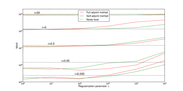
The observed behavior is similar to the one previously noted (but not plotted) for the idealized situation. Both methods behave identically in terms of cost decreasing for a $1\%$ noise level on the data. In all cases, they demonstrate a robust behavior that provides an optimal discrepancy (according to Morozov). The expected behavior of over-fitting (i.e. to reach a final misfit smaller than the one computed from the target friction coefficient with perturbed data) for $\gamma$ small enough suggests that the gradient provided by both methods is a priori accurate enough with regards to the noise level (unlike the slab case with smaller noise, see Figure 6). The peculiar behavior for the case $r=50$ where the discrepancy remains lower than the optimal one regardless of the regularization parameter $\gamma$ is detailed hereafter.

Figure 12 plots the DFT of the friction coefficients inferred by both methods and of the target coefficient (27) for a noise level of $1\%$ on the data and for the $5$ slip ratios $r$.

Abbildung 12: Discrete Fourier Transform for inferred friction coefficients $\beta_{f}$ and $\beta_{s}$ and for the target one $\beta_{r}$. Frequency $f_{3}$ is never captured by any method and is thus not plotted on the curves. A noise level $\delta=1\%$ is used in all situations.

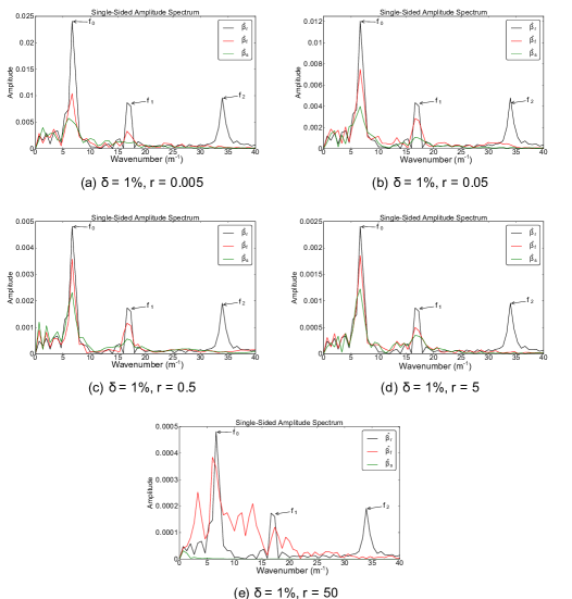
While the wavelengths considered in the friction coefficient (27) are similar (in terms of thickness ratio) to those considered for the quasi-uniform test case, the use of a higher noise on a non-uniform flow deteriorated the reconstruction at all levels. The carrier frequency amplitude (of wavelength $5h$) is never fully recovered by any method but clearly appears for $r\leq 5$. Likewise, frequency $f_{1}$ (of wavelength $2h$), well captured in previous simulations by the full adjoint method, is fairly well reconstructed only for $0.05\leq r\leq 5$. Again the “self-adjoint” method is able to recover it only partially. However, the interferences introduced by the “self-adjoint” method within the inferred friction coefficient do not appear anymore for this level of noise on the surface data. It therefore seems coherent with the limited accuracy of the gradient provided by this method.

As a consequence, the chosen frequencies for these simulations are too high to be recovered in this non-uniform flow with realistic data. Numerical experiments using higher wavelengths in the friction coefficient show that an accurate reconstruction for any slip ratio can be obtained, for the full adjoint method, for a carrier wave of wavelength $10h$ and a perturbation of wavelength $5h$ ; shorter wavelengths are not accessible.

What is of further interest is that the full adjoint method brings, in all cases, an enhanced and more faithful reconstruction of the friction coefficient for both the carrier wave and the first perturbation.

The pattern of behavior of the rapid sliding case ($r=50$) is different compared to the other cases. The full adjoint method retrieves roughly the carrier frequency with very high interferences (including one low frequency high amplitude interference) and the “self-adjoint” method does not capture any information of the target signal in addition to the initial guess.

In order to understand this phenomena, we plot in Figure 13 the gradients $\partial j/\partial\beta(\beta_{0})$ with $\beta$ defined by (31) for several average value $a$ of the friction coefficient, described in terms of slip ratio $r$. The computed gradients are evaluated around $\beta_{0}=a$.

Abbildung 13: Relative sensitivities to the friction coefficient with respect to the abscissa $x$ for various slip ratios, evaluated around the average value $a$.

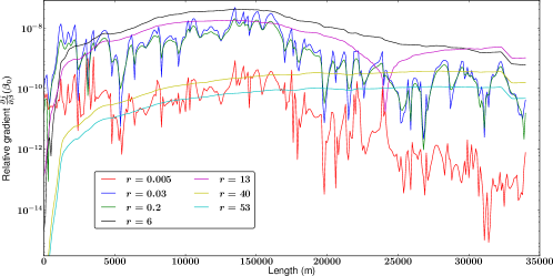
Increasing the slip ratio has a very clear effect on the sensitivities. For slip ratios $r<1$, the sensitivities include the local effects of the high frequencies contained in $\beta$, thus providing a highly variable gradient around an average behavior. The fact that the sensitivity decreases with $r$, due to poorer information transmission between the bottom and the surface, is recovered. It follows that, in the cases $r<1$, the limitations in the identification of all the frequencies of the friction coefficient come from the precision on the data.

The situations $r>1$ bring significantly smoother gradients. The cases $r=6$ and $r=13$, that still represent moderate slip ratios, contain a certain local variability but their rather smooth appearance shows a strong correlation with the global topography (or similarly the surface velocities, see Figure 9 and Figure 10) and the high frequencies of $\beta$ seem already erased from the gradient. In these situations, the main component resisting the flow is more the large scale (or equivalent) topography than the friction itself.

For higher slip ratios, the topographical effects seem to vanish as well, and the gradient only grows from the inflow boundary to the outflow boundary to reach a maximum value close to the right border. In the present case, one can deduce that the only effect resisting the flow is the cryostatic pressure considered on the right boundary.

A global decreasing of the sensitivity with increasing $r$ is also observed, reinforcing the existence of a sensitivity peak for in-between $r$. For $r>1$, it is not the quality of the data that prevents an accurate reconstruction of $\beta$ but the non-local behavior of the flow. When basal friction vanishes, it does not embody more than a small fraction of the global resistance to the flow. An extreme example is the progress of an ice-shelf on water where the friction resistance is close to zero. In the case of a tridimensional solution, stresses would be taken over by lateral shearing. In our case, these effects do not exist and it is the hydrostatic pressure boundary condition that resists the flow. These clearly non-local effects suggest than the flow can only be globally controlled, thus limiting the range of identifiable frequencies, regardless of data accuracy. Let us recall that, in terms of absolute errors, a higher slip ratio leads to a smaller absolute value of the friction coefficient and thus to a smaller amplitude of errors. We also point out that the vanishing of the sensitivities close to the left boundary is due to the Dirichlet boundary condition.

These phenomena imply a strong equifinality for friction coefficient lower than a certain value. This observation appears in the Morozov’s curves (see Figure 11) for the case $r=50$. Indeed, the discrepancies for both methods are smaller than the theoretical optimal one, even for very strong regularization ($\gamma$ large) providing almost constant $\beta$ around $\beta_{0}$. The initial cost itself, evaluated for a constant $\beta$ equal to the average value, is barely higher than the theoretical optimal cost. The associated minimization problem is ill-posed and the Tikhonov regularization on the gradient of $\beta$ does not allow to overcome this problem.

For the case $r=50$ and a regularization small enough (considering that the Morozov’s principle does not allow the optimal $\gamma$ value to be selected) it is noticeable that the full adjoint method is able to retrieve a small quantity of information, along with a large noise (optimal control problem obviously ill-posed) whereas the “self-adjoint” method does not provide anything else than the initial guess, irrespective of the value of $\gamma$.

4 Density of the data

The previous simulations have been performed using surface velocity data quite dense (one measurement every $dx$). This section deals with test cases identical to the previous section but using sparser (one measure point every $1$km) and thus more realistic data (corresponding to one ice thickness, see e.g. Gudmundsson and Raymond (2008)). This density corresponds to approximately $10$ times less measurement points than the previous case. We consider thereafter the following friction coefficient for the synthetic data:

$$\beta_{r}^{N}(x)=a+\frac{a}{2}\sin\left(\frac{2\pi x}{200dx}\right)+\frac{a}{5}\sum_{i=1}^{N}f_{i}(x)$$ (34)

with

$$f_{i}(x)=\sin\left(\frac{2\pi x}{w_{i}dx}\right)\mbox{ with }w_{1}=100,\leavevmode\nobreak\ w_{2}=50,\leavevmode\nobreak\ w_{3}=20,$$ (35)

and by extension, we set:

$$\boldsymbol{f_{0}}(x)=\sin\left(\frac{2\pi x}{w_{0}dx}\right)\mbox{ with }w_{0}=200.$$ (36)

The friction coefficient chosen for these simulation contains lower frequencies than the previous one, simulating a carrier wave of wavelength $20h$ perturbed by high frequencies of wavelengths $10h$, $5h$ and $2h$. These characteristics are summarized in Table 3. Results are plotted in Figure 14 for a noise level of $1\%$.

	$\boldsymbol{f_{0}}$	$f_{1}$	$f_{2}$	$f_{3}$
Wavelength w.r.t $h=1$km (thickness)	$20h$	$10h$	$5h$	$2h$
Wavelength w.r.t $dx=100$m (edge length)	$200dx$	$100dx$	$50dx$	$20dx$
Wavenumber w.r.t $L=33.3$km (domain length)	$1.66$m-1	$3.33$m-1	$6.66$m-1	$16.6$m-1

Tabelle 3: Characteristics of signal $\beta$ given by (34).

Abbildung 14: Discrete Fourier Transform for inferred friction coefficients $\beta_{f}$ and $\beta_{s}$ and for the target one $\beta_{r}$ for sparse data a $1\%$ noise level.

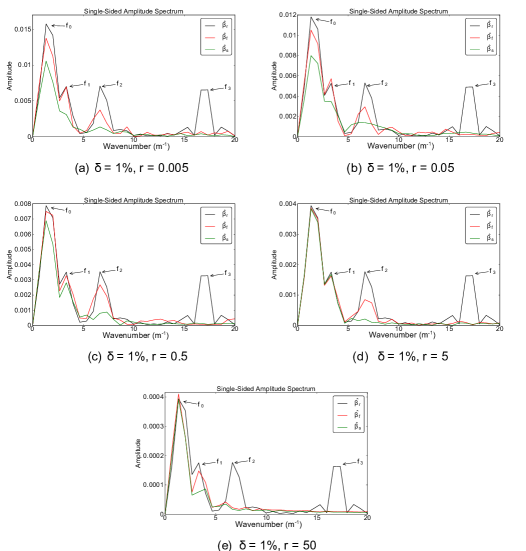
As a consequence, the level of identifiability assessed for dense data in the previous section is no longer valid. However, considering that one out of ten points has been retained, results seem rather convincing. The full adjoint method is able to accurately recover frequencies of wavelengths $20h$ and $10h$ (corresponding to $f_{0}$ and $f_{1}$) for all degrees of slip. The “self-adjoint” method recovers the carrier wave quite well although a stronger friction ($r\leq 0.05$) significantly degrades the reconstruction of the amplitude. Frequency $f_{1}$ is well captured for propitious situations ($0.5\leq r\leq 5$). Frequency $f_{2}$ (of wavelength $5h$, the lowest frequency considered in the dense data situation) is partially reconstructed by the full adjoint method for $r\leq 5$ and never captured by the “self-adjoint” method.

The case $r=50$ is a lot less problematic than previously found, due to lower frequencies and subsequently less local effects regarding the sharpness of the bed discretization. A pronounced difficulty appears for the identification of frequency $f_{1}$ (of wavelength $10h$). The case $r=50$ is the only one where frequency $f_{2}$ does not appear in the spectrum of $\widehat{\beta}_{f}$ (consistently to the previous simulations).

The significant time saving brought by the “self-adjoint” method due to its straightforward implementation is a favorable asset. However, its reliability is questionable and it seems important to know its limitations in order to perform realistic experiments.

The realistic simulation (low density data, $1\%$ noise, real topography, non-linear friction) allows us to assess the full adjoint method ability to accurately identify wavelengths greater or equal to $10$ ice thicknesses and to capture effects of wavelengths up to $5$ thicknesses for slip ratio lower than $5$. These bounds are defined by the level of noise considered on the data and a higher accuracy on the data would allow to identify higher frequencies.

The “self-adjoint” method , based on second order numerical schemes, while providing an incorrect gradient, is able to reconstruct wavelengths greater than $20$ ice thicknesses (with noticeable difficulties for strong friction). Wavelengths of $10$ ice thicknesses can be captured in propitious situations of intermediate sliding ($0.5\leq r\leq 5$). These bounds are strict and a lower noise would not allow to overcome the limited precision of the “self-adjoint” gradient.

The results provided by the full adjoint method are significantly better than those given by Petra et al. (2012) (who assess a limit of $20$ ice thicknesses for a non-linear rheology). It is difficult to compare considering that the authors provide neither their slip ratio nor the density of the data. In addition, the authors of Petra et al. (2012) consider a linear friction law.

The use of a non-linear friction allows us to simulate complex behaviors of the ice-bedrock interaction. This type of law can describe a non-linear deformation of the basal substrate or a non-linear response of the sliding velocity to the water pressure of sub-glacial cavities. The former reconstructions focus on the identification of a generic $\beta$. However one may confidently generalize these results to more complex sliding laws where $\beta$ would be identified through its parameterization (by a water pressure, a contact surface with sub-glacial cavities, a sedimentary roughness, a geothermal flux, …). It is important to recall that an identical cost $j$ does not mean an identical results due to the equifinality aspect and that over-parameterization is hardly ever in favor of an accurate identification; the identification of several parameters simultaneously would strongly reinforce the problem of equifinality (i.e. the ill-posedness of the inverse problem).

In other respect, we recall that the use of a “self-adjoint” gradient in the case of a non-linear friction law leads to ignore important extra contribution (compared to the case of a linear friction, see Section 2.2) in the gradient computation (see equation (23)) which adds even more discrepancy into the adjoint problem.

This work focuses on the identification of the friction coefficient that plays a major role to control the flow (i.e. the model shows a great sensitivity to the friction). The identification of a parameter such as the consistency $\eta_{0}$, for which the model sensitivity is significantly lower, needs to be done with caution for the full adjoint method (see e.g. Martin and Monnier (2014b)) and thus with increased caution for the “self-adjoint” method.

Finally, the adjoint obtained from source-to-source algorithmic differentiation allows us to simulate every level of needed precision between the best precision of the exact adjoint to the lowest one of the “self-adjoint” approximation. This leads to the consideration of an incomplete adjoint methodology where the approximation is completely adjustable, thus allowing the right compromise between CPU-time, memory burden and required accuracy to be achieved. Numerical experiments show that the retention of the last two states of the forward iterative loop (or equivalently the first two states of the reverse accumulation loop) within the gradient computation significantly improves its precision while maintaining a quite small computational burden. Let us recall that such an approach should be combine with an accurate solution for the forward problem

Anhang A Adjoint of a linear solver

This appendix describes how to generate the adjoint of a generic routine containing a call to a linear solver whose contents is a priori unknown.

The direct routine

A general direct routine can be described as follows. Let $c$ and $d$ be two given input parameters such that:

$$\left(\begin{array}[]{c}A\\ b\end{array}\right)=f(c,d)=\left(\begin{array}[]{c}f_{1}(c,d)\\ f_{2}(c,d)\end{array}\right)$$

with $A$ a matrix and $b$ a vector. Let $x$ be the solution of the linear system $Ax=b$ and $j$ defining a cost function evaluated at $x$. Figure 15 illustrates the direct routines dependencies.

Abbildung 15: Direct routine scheme

The linear tangent routine

The linear tangent routine associated to the direct routine described herebefore is then written:

$$\left(\begin{array}[]{c}\dot{A}\\ \dot{b}\end{array}\right)=df(c,d)\cdot\left(\begin{array}[]{c}\dot{c}\\ \dot{d}\end{array}\right)$$

where $df$ is the linear tangent model and $\dot{c}$ and $\dot{d}$ are the tangent variables corresponding to parameters $c$ and $d$. They serve as input parameters for the linear tangent model in order to compute $\dot{A}$ and $\dot{b}$. We can now differentiate the linear system operation $Ax=b$ to obtain the following linear tangent system:

$$A\dot{x}=\dot{b}-\dot{A}x.$$

The matrix $A$ and the vector $x$ are provided by the direct routine and the quantities $\dot{A}$ and $\dot{b}$ are given by the tangent linear routine. The linear solver is finally called, as a black-box, to solve this equation and to obtain the linear tangent unknown $\dot{x}$ where the gradient of the cost $\dot{j}$ can be evaluated. The quantity $\dot{x}$ represents the derivative value of $x$ at $(c,d)$ in a given direction $(\dot{c},\dot{d})$. The linear tangent routine is illustrated in Figure 16.

Abbildung 16: Linear tangent routine scheme

The generated adjoint routines

Let us recall that the adjoint code corresponds to the linear tangent code in a reverse order. It follows that the output variables of the the linear tangent routine are input variables for the adjoint routine. Therefore, the output variables of the adjoint routine are $\bar{c}$ and $\bar{d}$ and represent the adjoint variables of $(c,d)$ (and are consequently of same type and size). The adjoint cost $\bar{j}$ is the input variable of the adjoint cost function and similarly, the adjoint state $\bar{x}$ is the input variable of the adjoint linear system.

The computation of the adjoint state can be split into three steps (see Fig. 16):

1. From $\bar{j}$, obtain $\bar{x}$ (generally provided by an independent routine called the adjoint cost function)

2. From $\bar{x}$, obtain $\bar{A}$ and $\bar{b}$

3. From $\bar{A}$ and $\bar{b}$, obtain $\bar{c}$ and $\bar{d}$ using the adjoint model $df^{*}$ such that:

   $$\left(\begin{array}[]{c}\bar{c}\\ \bar{d}\end{array}\right)=df^{*}(c,d)\cdot\left(\begin{array}[]{c}\bar{A}\\ \bar{b}\end{array}\right).$$

The adjoint of the linear system

The linear solver call occurs in the second step. The input variable is $\bar{x}$ and the output variables are $\bar{A}$ and $\bar{b}$. In the linear tangent code, we have: $A\dot{x}=\dot{b}-\dot{A}x$ or if one splits it into two steps:

$$\begin{array}[]{lcl}2a.&\dot{b^{\prime}}&=\dot{b}-\dot{A}x,\\ 2b.&A\dot{x}&=\dot{b^{\prime}}.\end{array}$$

An adjoint calculation being performed in the reverse order, the adjoint of this procedure starts with instruction $2b$ which can be written as follows:

$$\left(\begin{array}[]{c}\dot{x}\\ \dot{b}^{\prime}\end{array}\right)=\left(\begin{array}[]{ccc}0&A^{-1}\\ 0&1\end{array}\right)\times\left(\begin{array}[]{c}\dot{x}\\ \dot{b}^{\prime}\end{array}\right)\,.$$

Since $\dot{b^{\prime}}$ is the input variable for the instruction $2b$, its adjoint counterpart $\bar{b}^{\prime}$ is the output of the adjoint instruction of $2b$ (by convention, the adjoint output variables are set to $0$ before entering the adjoint routine). Similarly, since $\dot{x}$ is the output variable, its adjoint counterpart $\bar{x}$ is an input one. The adjoint instruction of step $2b$ are then written:

$$\left(\begin{array}[]{c}\bar{x}\\ \bar{b}^{\prime}\end{array}\right)=\left(\begin{array}[]{ccc}0&0\\ A^{-T}&1\end{array}\right)\times\left(\begin{array}[]{c}\bar{x}\\ \bar{b}^{\prime}\end{array}\right)\,.$$

The variable $\bar{b}^{\prime}$ is an output variable, hence set to $0$ before entering the adjoint routine. This operation corresponds to solving the linear system $A^{T}\bar{b}^{\prime}=\bar{x}$ in order to obtain $\bar{b}^{\prime}$ (using the linear solver).

Once $\bar{b}^{\prime}$ has been computed, one has to perform the adjoint of the instruction $2a)$. This instruction can be written as the following linear operation:

$$(\dot{b}^{\prime},\dot{b},\dot{A})=(\dot{b}^{\prime},\dot{b},\dot{A})\times\left(\begin{array}[]{ccc}0&0&0\\ 1&1&0\\ -x&0&1\end{array}\right).$$

The corresponding adjoint instruction is written:

$$(\bar{b}^{\prime},\bar{b},\bar{A})=(\bar{b}^{\prime},\bar{b},\bar{A})\times\left(\begin{array}[]{ccc}0&1&-x^{T}\\ 0&1&0\\ 0&0&1\end{array}\right)$$

which leads, in reverse order, to perform the following operations:

$$\left\{\begin{array}[]{rcl}\bar{b}&=&\bar{b}^{\prime},\\ \bar{A}&=&-\bar{b}x^{T}.\\ \end{array}\right.$$

The variables $\bar{A},\leavevmode\nobreak\ \bar{b}$ are output variables, hence set to $0$ before entering the adjoint routine and $\bar{b}^{\prime}$ has been obtained from the previous step (the adjoint of step $2b$).

In summary, the adjoint of the tangent linear instructions $A\dot{x}=\dot{b}-\dot{A}x$ (referred as step 2)) can be written:

$$\left\{\begin{array}[]{rcl}A^{T}\bar{b}&=&\bar{x},\\ \bar{A}&=&-\bar{b}x^{T},\\ \bar{x}&=&0.\\ \end{array}\right.$$

where $(\bar{c},\bar{d})$ are the components of the gradient with respect to $(c,d)$ obtained from the adjoint model $df^{*}$. The first instruction can then be solved using the same linear solver as the one used in the direct routine. The second instruction is written: $\bar{A}_{ij}=-\bar{b}_{i}x_{j}$.

Let us point out that the matrix $\bar{A}$ is of the same type as $A$ with the same sparse profile (even if $-\bar{b}x^{T}$ is a priori a full matrix). Therefore, only the adjoint values of coefficients $A_{i,j}$ are required.

The steps of the adjoint routine are illustrated in Figure 17.

Abbildung 17: Adjoint routine representation