Generalized Canonical Correlation Analysis and Its Application to Blind Source Separation Based on a Dual-Linear Predictor Structure

Abstract

Blind source separation (BSS) is one of the most important and established research topics in signal processing and many algorithms have been proposed based on different statistical properties of the source signals. For second-order statistics (SOS) based methods, canonical correlation analysis (CCA) has been proved to be an effective solution to the problem. In this work, the CCA approach is generalized to accommodate the case with added white noise and it is then applied to the BSS problem for noisy mixtures. In this approach, the noise component is assumed to be spatially and temporally white, but the variance information of noise is not required. An adaptive blind source extraction algorithm is derived based on this idea and a further extension is proposed by employing a dual-linear predictor structure for blind source extraction (BSE).

I INTRODUCTION

The problem of blind source separation (BSS) has been studied extensively in the past and a plethora of algorithms have been proposed in the past based on statistical properties of the source signals [1, 2]. For those based on the second-order statistics (SOS), one particular class of them is those based on the canonical correlation analysis (CCA) approach [3, 4, 5, 6, 7, 8, 9, 10, 11], where the demixing matrix is found by maximizing the autocorrelation of each of the recovered signals. This approach rests on the idea that the sum of any uncorrelated signals has an autocorrelation whose value is less or equal to the maximum value of individual signals. As shown in [8], the maximization of the autocorrelation value is equivalent to finding the generalised eigenvectors within the matrix pencil approach [12].

As shown in  [8], the CCA approach will work for the noise-free situations. For noisy mixtures, its performance will no doubt degrade. If we can estimate the variance of white noise in the mixtures, then we can remove the effect of noise from the mixtures before applying the noise-free BSS algorithms [13, 14]. However, the variance of noise in the mixtures is not always available and in this case the algorithm proposed in  [14] will not work.

In this paper, we will generalise the traditional CCA to include the case with noise and then apply it to the separation problem of noisy mixtures [15, 16]. A key advantage of this approach is that successful separation of source signals can be achieved without estimation of the white noise parameters. An online adaptive algorithm is derived accordingly as its adaptive realisation.

Moreover, similar to the CCA case [8], we have also related the GCCA approach to a dual-linear predictor based blind source extraction (BSE) structure, and an adaptive algorithm based on such a structure is also derived with rigorous proof for its effectiveness in this context.

This paper is organised as follows. In Section II, the generalised CCA approach will be provided with a detailed proof and analysis about its condition on which it can be applied to the BSS problem. The class of adaptive BSE algorithms is derived in Sec. III. Simulation results are shown in Section IV and conclusions drawn in Section V.

II Generalised CCA and Its Application to BSS

II-A Overview of the CCA Approach to BSS

The instantaneous mixing problem in BSS with $M$ mixtures, $L$ sources and a mixing matrix ${\bf A}$ can be expressed as

$${\bf x}[n]={\bf A}\cdot{\bf s}[n],$$ (1)

with

$${\bf s}[n] = \left[s_{0}[n]\;s_{1}[n]\;\cdots\;s_{L\!-\!1}[n]\right]^{\mathrm{T}}$$

$${\bf x}[n] = \left[x_{0}[n]\;x_{1}[n]\;\cdots\;x_{M\!-\!1}[n]\right]^{\mathrm{T}}$$

$$\left[{\bf A}\right]_{m,l} = a_{m,l}\;,m=0,\dots,M-1,\;l=0,\dots,L-1.$$ (2)

For BSS employing second-order statistics (SOS), we assume the sources are spatially uncorrelated and have different temporal structures:

$${\bf R}_{ss}[0] = E\{{\bf s}[n]{\bf s}^{T}[n]\}=\mbox{diag}\{\rho_{0}[0],\rho_{1}[0],\dots,\rho_{L-1}[0]\}$$

$${\bf R}_{ss}[\Delta n] = E\{{\bf s}[n]{\bf s}^{T}[n-\Delta n]\}=\mbox{diag}\{\rho_{0}[\Delta n],\rho_{1}[\Delta n],\dots,\rho_{L-1}[\Delta n]\}$$ (3)

with $\rho_{l}[n]$ being the autocorrelation function of the $l$th source signal and $\rho_{l}[\Delta n]\neq 0$ for some nonzero delays $\Delta n$.

The BSS problem can be solved in one single step by the CCA approach. In CCA [17], two sets of zero-mean variables ${\bf z}_{1}[n]$ (with $q_{1}$ components) and ${\bf z}_{2}[n]$ (with $q_{2}$ components) with a joint distribution are considered. For convenience, we assume $q_{1}\leq q_{2}$. The linear combination of the variables in each of the vectors is respectively given by

$$a_{0}[n] = \boldsymbol{\alpha}_{0}^{T}{\bf z}_{1}[n]$$

$$b_{0}[n] = \boldsymbol{\beta}_{0}^{T}{\bf z}_{2}[n]\;,$$ (4)

where $\boldsymbol{\alpha}_{0}$ and $\boldsymbol{\beta}_{0}$ are vectors containing the combination coefficients and they are determined by maximizing the correlation between $a_{0}$ and $b_{0}$

$$\max_{\boldsymbol{\alpha}_{0},\boldsymbol{\beta}_{0}}J_{0}(\boldsymbol{\alpha}_{0},\boldsymbol{\beta}_{0})\;$$ (5)

with

$$J_{0}(\boldsymbol{\alpha}_{0},\boldsymbol{\beta}_{0}) = \frac{E\{a_{0}[n]b_{0}[n]\}}{\sqrt{E\{a_{0}^{2}[n]\}E\{b_{0}^{2}[n]\}}}$$ (6)

$$= \frac{\boldsymbol{\alpha}_{0}^{T}\boldsymbol{\Sigma}_{12}\boldsymbol{\beta}_{0}}{\sqrt{(\boldsymbol{\alpha}_{0}^{T}\boldsymbol{\Sigma}_{11}[0]\boldsymbol{\alpha}_{0})(\boldsymbol{\beta}_{0}^{T}\boldsymbol{\Sigma}_{22}[0]\boldsymbol{\beta}_{0})}}\;,$$

where $\boldsymbol{\Sigma}_{11}[0]=E\{{\bf z}_{1}[n]{\bf z}_{1}^{T}[n]\}$, $\boldsymbol{\Sigma}_{12}=E\{{\bf z}_{1}[n]{\bf z}_{2}^{T}[n]\}$, $\boldsymbol{\Sigma}_{22}=E\{{\bf z}_{2}[n]{\bf z}_{2}^{T}[n]\}$ and $E\{\cdot\}$ denotes the statistical expectation operator.

After finding the first pair of optimal vectors $\boldsymbol{\alpha}_{0}$ and $\boldsymbol{\beta}_{0}$, we can proceed to find the second pair $\boldsymbol{\alpha}_{1}$ and $\boldsymbol{\beta}_{1}$ which maximizes the correlation and at the same time ensures that the new pair of combinations $\{a_{1}[n],\;b_{1}[n]\}$ is uncorrelated with the first set $\{a_{0}[n],\;b_{0}[n]\}$. This process is repeated until we find all the $\min(q_{1},q_{2})=q_{1}$ pairs of optimal vectors $\boldsymbol{\alpha}_{i}$ and $\boldsymbol{\beta}_{i}$, $i=0$, $\dots$, $q_{1}-1$.

It has been shown that $\boldsymbol{\alpha}_{i}$ can be obtained by solving the following generalized eigenvalue problem [8]

$$\boldsymbol{\Sigma}_{12}\boldsymbol{\Sigma}_{22}^{-1}\boldsymbol{\Sigma}_{21}\boldsymbol{\alpha}_{i}=\lambda_{i}^{2}\boldsymbol{\Sigma}_{11}\boldsymbol{\alpha}_{i}\;.$$ (7)

$\boldsymbol{\beta}_{i}$ can be found in the same way by changing the subscripts of the matrices in (7) accordingly.

To apply CCA to the BSS problem [8], we choose the vector ${\bf x}[n]$ as ${\bf z}_{1}$ in CCA and ${\bf x}[n-\Delta_{n}]$ as ${\bf z}_{2}$. Then the eigenvalue problem in (7) becomes

$${\bf R}_{xx}[\Delta n]{\bf R}_{xx}[0]^{-1}{\bf R}_{xx}[\Delta n]\boldsymbol{\alpha}_{i}=\lambda_{i}^{2}{\bf R}_{xx}[0]\boldsymbol{\alpha}_{i}\;.$$ (8)

In the context of BSS, $\boldsymbol{\alpha}_{i}$ and $\boldsymbol{\beta}_{i}$ are the same and we use ${\bf w}_{i}$ to represent it. (8) can be simplified as

$${\bf R}_{xx}[0]^{-1}{\bf R}_{xx}[\Delta n]{\bf w}_{i}=\lambda_{i}{\bf w}_{i}\;.$$ (9)

Multiplying both sides with ${\bf R}_{xx}[0]$, we arrive at the following generalised eigenvector problem

$${\bf R}_{xx}[\Delta n]{\bf w}_{i}=\lambda_{i}{\bf R}_{xx}[0]{\bf w}_{i}\;.$$ (10)

Moreover, the correlation maximization problem in (5) becomes

$$\max_{{\bf w}_{0}}J_{0}({\bf w}_{0})=\frac{{\bf w}_{0}^{T}{\bf R}_{xx}[\Delta n]{\bf w}_{0}}{{\bf w}_{0}^{T}{\bf R}_{xx}[0]{\bf w}_{0}}=\frac{{\bf w}_{0}^{T}{\bf A}{\bf R}_{ss}[\Delta n]{\bf A}^{T}{\bf w}_{0}}{{\bf w}_{0}^{T}{\bf A}{\bf R}_{ss}[0]{\bf A}^{T}{\bf w}_{0}}\;,$$ (11)

and we can prove that by CCA the source signals will be recovered completely [8]. However, with added noise, the proof given in the noise-free case will not be valid any more since the denominator in (6) will have a noise component. As a result, the performance of the CCA approach will degrade with increasing noise level.

II-B Generalised CCA (GCCA)

For noisy mixtures, ${\bf x}[n]$ is given by

$${\bf x}[n]={\bf A}{\bf s}[n]+{\bf v}[n],$$ (12)

where ${\bf v}[n]$ is the additive noise vector, which is spatially and temporally white and uncorrelated with the source signals. Its correlation matrix is given by

$${\bf R}_{vv}[\Delta_{n}]=E\{{\bf v}[n]{\bf v}^{T}[n-\Delta_{n}]\}=\left\{\begin{array}[]{ll}{\bf 0}&\mbox{for }\Delta_{n}\neq 0\\ \sigma_{v}^{2}{\bf I}&\mbox{for }\Delta_{n}=0\end{array}\right..$$ (13)

where ${\bf I}$ is the identity matrix and $\sigma_{v}^{2}$ is the variance of noise.

Similarly, we can form a modified CCA problem for two set of variables with added white noise. Now consider the two sets of zero-mean variables

$$\hat{{\bf z}}_{1}[n] = {\bf z}_{1}[n]+{\bf v}_{1}[n]$$

$$\hat{{\bf z}}_{2}[n] = {\bf z}_{2}[n]+{\bf v}_{2}[n]$$ (14)

and their corresponding linear combinations:

$$\hat{a}_{0}[n] = \boldsymbol{\alpha}_{0}^{T}\hat{{\bf z}}_{1}[n]$$

$$\hat{b}_{0}[n] = \boldsymbol{\beta}_{0}^{T}\hat{{\bf z}}_{2}[n]\;,$$ (15)

where ${\bf v}_{1}$ and ${\bf v}_{2}$ are the added white noise vectors and not correlated with each other. Now the two vectors $\boldsymbol{\alpha}_{0}$ and $\boldsymbol{\beta}_{0}$ are not given by (5) any more, but by

$$\max_{\boldsymbol{\alpha}_{0},\boldsymbol{\beta}_{0}}\hat{J}_{0}(\boldsymbol{\alpha}_{0},\boldsymbol{\beta}_{0})\;$$ (16)

with

$$\hat{J}_{0}(\boldsymbol{\alpha}_{0},\boldsymbol{\beta}_{0}) = \frac{E\{\hat{a}_{0}[n]\hat{b}_{0}[n]\}}{E\{\hat{a}_{0}[n]\hat{a}_{0}[n-\Delta_{0}]\}E\{\hat{b}_{0}[n]\hat{b}_{0}[n-\Delta_{0}]\}}$$ (17)

$$= \frac{\boldsymbol{\alpha}_{0}^{T}\hat{\boldsymbol{\Sigma}}_{12}\boldsymbol{\beta}_{0}}{\sqrt{(\boldsymbol{\alpha}_{0}^{T}\hat{\boldsymbol{\Sigma}}_{11}[\Delta_{0}]\boldsymbol{\alpha}_{0})(\boldsymbol{\beta}_{0}^{T}\hat{\boldsymbol{\Sigma}}_{22}[\Delta_{0}]\boldsymbol{\beta}_{0})}}\;,$$

where $\hat{\boldsymbol{\Sigma}}_{12}=E\{\hat{{\bf z}}_{1}[n]\hat{{\bf z}}_{2}^{T}[n]\}$, $\hat{\boldsymbol{\Sigma}}_{11}[\Delta_{0}]=E\{\hat{{\bf z}}_{1}[n]\hat{{\bf z}}_{1}^{T}[n-\Delta_{0}]\}$, $\hat{\boldsymbol{\Sigma}}_{22}[\Delta_{0}]=E\{\hat{{\bf z}}_{2}[n]\hat{{\bf z}}_{2}^{T}[n-\Delta_{0}]\}$ and $\Delta_{0}$ is a non-zero integer. In this new function, the correlation between the two variables $a_{0}[n]$ and $b_{0}[n]$ is not normalised by their variances, but by their own correlation for a common time lag of $\Delta_{0}$. $\boldsymbol{\alpha}_{i}$ and $\boldsymbol{\beta}_{i}$, $i=0,1,\dots,q_{1}-1$, are all obtained in a similar way with the same normalisation. Since the noise components are not correlated with each other and not correlated with ${\bf z}_{1}$ and ${\bf z}_{2}$ either, we have $\hat{\boldsymbol{\Sigma}}_{12}=\boldsymbol{\Sigma}_{12}$ and for nonzero $\Delta_{0}$, the denominator in (17) does not include any noise information. So although there is noise component existing in the original variables, the vectors $\boldsymbol{\alpha}_{i}$ and $\boldsymbol{\beta}_{i}$ obtained in this way will not depend on the noise component at all. So the effect of noise has been removed without estimating its variances.

II-C Applying GCCA to the BSS Problem

Applying this generalised CCA to the BSS problem, we can replace $\hat{{\bf z}}_{1}[n]$ by ${\bf x}[n]$ in (12) and $\hat{{\bf z}}_{2}[n]$ by ${\bf x}[n-\Delta_{1}]$ with $\Delta_{1}\neq\Delta_{0}$. The two vectors $\boldsymbol{\alpha}_{0}$ and $\boldsymbol{\beta}_{0}$ will be the same as the extraction vector ${\bf w}_{0}$ [8]. The extracted signal will be

$$y_{0}[n]={\bf w}_{0}^{T}{\bf x}[n]\;.$$ (18)

Then the maximization problem in (16) becomes

$$\max_{{\bf w}_{0}}\hat{J}_{0}({\bf w}_{0})\;,$$ (19)

with

$$\hat{J}_{0}({\bf w}_{0})=\frac{E\{y_{0}[n]y_{0}[n-\Delta_{1}]\}}{E\{y_{0}[n]y_{0}[n-\Delta_{0}]\}}=\frac{{\bf w}_{0}^{T}{\bf R}_{xx}[\Delta_{1}]{\bf w}_{0}}{{\bf w}_{0}^{T}{\bf R}_{xx}[\Delta_{0}]{\bf w}_{0}}\;,$$ (20)

where ${\bf R}_{xx}[\Delta_{i}]=E\{{\bf x}[n]{\bf x}[n-\Delta_{i}]^{T}\}$, $i=0,1$, is the correlation matrix of the observed mixtures. From (12), we have

$${\bf R}_{xx}[\Delta_{i}] = {\bf A}E\{{\bf s}[n]{\bf s}^{T}[n-\Delta_{i}]\}{\bf A}^{T}$$ (21)

$$+E\{{\bf v}[n]{\bf v}^{T}[n-\Delta_{i}]\}$$

$$= {\bf A}{\bf R}_{ss}[\Delta_{i}]{\bf A}^{T}\;,$$

since ${\bf R}_{vv}[\Delta_{i}]=0$ for $\Delta_{i}\neq 0$.

So the cost function $\hat{J}_{0}$ can be further simplified to

$$\hat{J}_{0}({\bf w}_{0})=\frac{{\bf w}_{0}^{T}{\bf A}{\bf R}_{ss}[\Delta_{1}]{\bf A}^{T}{\bf w}_{0}}{{\bf w}_{0}^{T}{\bf A}{\bf R}_{ss}[\Delta_{0}]{\bf A}^{T}{\bf w}_{0}}\;.$$ (22)

We assume that all of the diagonal elements of ${\bf R}_{ss}[\Delta_{0}]$ are positive, which means each of the source signals themselves should have a positive correlation value with its delayed version by $\Delta_{0}$.

In the next, we give a brief proof that maximization of $\hat{J}_{0}({\bf w}_{0})$ with respect to ${\bf w}_{0}$ will lead to a successful extraction of one of the source signals in the presence of noise.

Let ${\bf g}_{0}={\bf A}^{T}{\bf w}_{0}$ denote the first global mixing vector. Then $\hat{J}_{0}({\bf w}_{0})$ in (22) changes into

$$\hat{J}_{0}({\bf w}_{0})=\frac{{\bf g}_{0}^{T}{\bf R}_{ss}[\Delta_{1}]{\bf g}_{0}}{{\bf g}_{0}^{T}{\bf R}_{ss}[\Delta_{0}]{\bf g}_{0}}\;.$$ (23)

Since all of the diagonal elements of the diagonal matrix ${\bf R}_{ss}[\Delta_{0}]$ are positive, we shall assume ${\bf R}_{ss}[\Delta_{0}]={\bf I}$, as the differences in the diagonal elements of ${\bf R}_{ss}[\Delta_{0}]$ can always be absorbed into the mixing matrix ${\bf A}$. This way, the diagonal elements of ${\bf R}_{ss}[\Delta_{1}]$ become the “normalised” autocorrelation values of each source signal and they are assumed to be different from each other. Note the “normalisation” here is not by $E\{s^{2}_{l}[n]\}$, but by $E\{s_{l}[n]s_{l}[n-\Delta_{0}]\}$, $l=0,1,\dots,L-1$. Now we have

$$J_{0}({\bf w}_{0})=\hat{{\bf g}}_{0}^{T}{\bf R}_{ss}[\Delta_{l}]\hat{{\bf g}}_{0}\;,$$ (24)

where $\hat{{\bf g}}_{0}=\frac{{\bf g}_{0}}{\sqrt{{\bf g}_{0}^{T}{\bf g}_{0}}}$, which has a property $\hat{{\bf g}}_{0}^{T}\hat{{\bf g}}_{0}=1$.

This is an eigenvalue problem and starting from here, we can use the results given in [8] to complete the proof and draw the conclusion that when we maximize $\hat{J}_{0}({\bf w}_{0})$ with respect to ${\bf w}_{0}$, this will result in a successful extraction of the source signal with the maximum “normalised” autocorrelation value.

After extracting the first source signal, we may use a deflation approach to remove it from the mixtures and then subsequently perform the next extraction [2]. This procedure is repeated until the last source signal is recovered.

III Adaptive Realisation

III-A A direction approach

As in the noise-free case [8], from the proof we can see that both the correlation matrix in both the numerator and the denominator in the cost function $\hat{J}_{0}$ can be replaced by a linear combination of the correlation matrices at different time lags to improve its robustness, as long as the one at the denominator is positive definite. More specifically, instead of maximizing the correlation between $y_{0}[n]$ and $y_{0}[n-\Delta_{1}]$, we maximize the correlation between $y_{0}[n]$ and a weighted sum of $y_{0}[n-p]$, $p=2,3,\dots,P+1$ [16]. Now the new cost function is given by

$$J({\bf w}_{0})=\frac{E\{y_{0}[n]e_{0}[n]\}}{E\{y_{0}[n]y_{0}[n-1]\}}\;,$$ (25)

where

$$e_{0}[n]={\bf b}^{T}{\bf y}_{0}[n]$$ (26)

with

$${\bf b} = \left[b_{1}\;b_{2}\;\cdots\;b_{P}\right]^{\mathrm{T}}$$

$${\bf y}_{0}[n] = \left[y_{0}[n-2]\;y_{0}[n-3]\cdots y_{0}[n\!-P\!-1]\right]^{\mathrm{T}}$$ (27)

As shown in (25), we have chosen $\Delta_{0}=1$ because in reality more likely the signal is positively correlated with its delayed version by one sample.

Applying the standard gradient descent method to $J_{0}({\bf w}_{0},{\bf b})$, we have

$$\nabla_{{\bf w}_{0}}J = \frac{1}{E\{y_{0}[n]y_{0}[n-1]\}^{2}}\left(E\{y_{0}[n]\hat{{\bf x}}[n]+\right.$$ (28)

$${\bf x}[n]e_{0}[n]\}E\{y_{0}[n]y_{0}[n-1]\}-$$

$$\left.E\{y_{0}[n]e_{0}[n]\}E\{y_{0}[n]{\bf x}[n-1]+{\bf x}[n]y_{0}[n-1]\}\right)$$

where

$$\hat{{\bf x}}[n]=\sum_{p=2}^{P+1}b_{p}{\bf x}[n-p]\;.$$ (29)

The correlation $E\{y_{0}[n]y_{0}[n-1]\}$ can be estimated recursively by

$$\sigma_{y}[n] = \beta\sigma_{y}[n-1]+(1-\beta)y_{0}[n]y_{0}[n-1]\;,$$ (30)

where$\beta$ is the corresponding forgetting factor with $0\leq\beta<1$.

Following some standard stochastic approximation techniques [18], we obtain the following online update equation

$${\bf w}_{0}[n+1]\!\! =\!\! {\bf w}_{0}[n]+$$ (31)

$$\frac{\mu}{\sigma_{y}^{2}}\left((y_{0}[n]\hat{{\bf x}}[n]+{\bf x}[n]e_{0}[n])(y_{0}[n]y_{0}[n-1])-\right.$$

$$\left.(y_{0}[n]e_{0}[n])(y_{0}[n]{\bf x}[n-1]+{\bf x}[n]y_{0}[n-1])\right)$$

where $\mu$ is the updating step size.

To avoid the critical case where the norm of ${\bf w}_{0}[n]$ becomes too small, after each update, we normalize it to unit length, which yields

$${\bf w}_{0}[n+1]\leftarrow{\bf w}_{0}[n+1]/\sqrt{{\bf w}_{0}^{T}[n+1]{\bf w}_{0}[n+1]}\;.$$ (32)

III-B Adaptive Realisation Based on the Dual-Linear Predictor Structure

For noise-free mixtures, a linear predictor can be employed to extract one of the sources [19, 20, 21, 22], and it is closely related to the CCA approach, as shown in [8]. Similarly, for the GCCA approach, we can develop a corresponding dual-linear predictor structure for its implementation [15].

III-B1 The Structure

Figure 1: A linear predictor based BSE structure.

For noise-free mixtures, a linear predictor can be employed to extract one of the sources, as shown in Figure 1, where the extracted signal $y[n]$ and the instantaneous output error $e[n]$ of the linear predictor with a length $P$ are given by

$$y[n] = {\bf w}^{T}{\bf x}[n]$$

$$e[n] = y[n]-{\bf b}^{T}{\bf y}[n]\;,$$ (33)

where ${\bf w}$ is the demixing vector and

$${\bf b} = \left[b_{1}\;b_{2}\;\cdots\;b_{P}\right]^{\mathrm{T}}$$

$${\bf y}[n] = \left[y[n-1]\;y[n-2]\;\cdots\;y[n\!-P]\right]^{\mathrm{T}}\;.$$ (34)

The cost function is given by

$$J_{0}({\bf w})=\frac{E\{e^{2}[n]\}}{E\{y^{2}[n]\}}\;.$$ (35)

As proved in [21], by minimising $J_{0}({\bf w})$ with respect to ${\bf w}$, the sources can be extracted successfully.

Figure 2: The proposed dual-linear predictor structure for BSE.

However, in the presence of noise, there will be a noise term in both the numerator and the denominator of (35) and the proof in [21] is not valid any more. To remove the effect of noise, as in GCCA, we propose to exploit the white nature of the noise components and employ a dual-linear predictor structure as shown in Fig. 2, where a second linear predictor with coefficients vector ${\bf d}$ of length $P_{d}$ is employed and the error signal $f[n]$ is given by

$$f[n] = y[n]-{\bf d}^{T}{\bf y}_{d}[n]\;,$$ (36)

where

$${\bf d} = \left[b_{1}\;b_{2}\;\cdots\;b_{P_{d}}\right]^{\mathrm{T}}$$

$${\bf y}_{d}[n] = \left[y[n-1]\;y[n-2]\;\cdots\;y[n\!-P_{d}]\right]^{\mathrm{T}}\;.$$ (37)

For the first linear predictor, the mean square prediction error (MSPE) $E\{e^{2}[n]\}$ is given by

$$E\{e^{2}[n]\} = E\{y^{2}[n]\}-2E\{y[n]{\bf b}^{T}{\bf y}[n]\}+$$ (38)

$$E\{{\bf b}^{T}{\bf y}[n]{\bf y}^{T}[n]{\bf b}\}$$

$$= \sum_{p=0}^{P}b_{p}^{2}E\{y^{2}[n-p]\}-$$

$$\sum_{p,q=0;p\neq q}^{P}s_{pq}b_{p}b_{q}E\{y[n-p]y[n-q]\}$$

$$= q_{c}E\{y^{2}[n]\}-$$

$$\sum_{p,q=0;p\neq q}^{P}s_{pq}b_{p}b_{q}{\bf w}^{T}{\bf R}_{xx}[q-p]{\bf w}$$

$$= q_{c}E\{y^{2}[n]\}-$$

$${\bf w}^{T}(\sum_{p,q=0;p\neq q}^{P}s_{pq}b_{p}b_{q}{\bf R}_{xx}[q-p]){\bf w}\;,$$

where $q_{c}=\sum_{p=0}^{P}b_{p}^{2}$ with $b_{0}=1$, and $s_{pq}$ is $1$ when $p=0$ or $q=0$, and $-1$ otherwise. From (12), (13) and (3), we have

$${\bf R}_{xx}[p-q] = {\bf A}E\{{\bf s}[n]{\bf s}^{T}[n-(p-q)]\}{\bf A}^{T}$$ (39)

$$+E\{{\bf v}[n]{\bf v}^{T}[n-(p-q)]\}$$

$$= {\bf A}{\bf R}_{ss}[p-q]{\bf A}^{T}\;,$$

for $p\neq q$. Then we have

$$E\{e^{2}[n]\} = q_{c}E\{y^{2}[n]\}-$$ (40)

$${\bf w}^{T}{\bf A}(\sum_{p,q=0;p\neq q}^{P}s_{pq}b_{p}b_{q}{\bf R}_{ss}[q-p]){\bf A}^{T}{\bf w}$$

$$= q_{c}E\{y^{2}[n]\}-$$

$${\bf g}^{T}(\sum_{p,q=0;p\neq q}^{P}s_{pq}b_{p}b_{q}{\bf R}_{ss}[q-p]){\bf g}$$

$$= q_{c}E\{y^{2}[n]\}-{\bf g}^{T}\hat{{\bf R}}_{ss}{\bf g}\;,$$

with ${\bf g}={\bf A}^{T}{\bf w}$ denoting the global demixing vector and $\hat{{\bf R}}_{ss}$ is a diagonal matrix given by

$$\hat{{\bf R}}_{ss}=\sum_{p,q=0;p\neq q}^{P}s_{pq}b_{p}b_{q}{\bf R}_{ss}[q-p]\;,$$ (41)

with its $l-th$ diagonal element $\hat{r}_{l}$ given by

$$\hat{r}_{l}=\sum_{p,q=0;p\neq q}^{P}s_{pq}b_{p}b_{q}\rho_{l}[q-p]\;.$$ (42)

Similarly, for the second linear predictor, we have

$$E\{f^{2}[n]\} = E\{y^{2}[n]\}-2E\{y[n]{\bf d}^{T}{\bf y}_{d}[n]\}+$$ (43)

$$E\{{\bf d}^{T}{\bf y}_{d}[n]{\bf y}_{d}^{T}[n]{\bf d}\}$$

$$= a_{c}E\{y^{2}[n]\}-$$

$${\bf g}^{T}(\sum_{p,q=0;p\neq q}^{P_{d}}s_{pq}d_{p}d_{q}{\bf R}_{ss}[q-p]){\bf g}$$

$$= a_{c}E\{y^{2}[n]\}-{\bf g}^{T}\tilde{{\bf R}}_{ss}{\bf g}\;,$$

with $a_{c}=\sum_{p=0}^{P_{d}}d_{p}^{2}$ with $d_{0}=1$ and $\tilde{{\bf R}}_{ss}$ is a diagonal matrix given by

$$\tilde{{\bf R}}_{ss}=\sum_{p,q=0;p\neq q}^{P_{d}}s_{pq}d_{p}d_{q}{\bf R}_{ss}[q-p]\;,$$ (44)

with its $l-th$ diagonal element $\tilde{r}_{l}$ given by

$$\tilde{r}_{l}=\sum_{p,q=0;p\neq q}^{P_{d}}s_{pq}d_{p}d_{q}\rho_{l}[q-p]\;.$$ (45)

III-B2 The Proposed Cost Function

Note in the second term of both (40) and (43), there is not any noise component. Then we can construct a new cost function as follows

$$J({\bf w})=\frac{q_{c}E\{y^{2}[n]\}-E\{e^{2}[n]\}}{a_{c}E\{y^{2}[n]\}-E\{f^{2}[n]\}}=\frac{{\bf g}^{T}\hat{{\bf R}}_{ss}{\bf g}}{{\bf g}^{T}\tilde{{\bf R}}_{ss}{\bf g}}\;.$$ (46)

Now we impose another condition on the second linear predictor: suppose the coefficients ${\bf d}$ are chosen in such a way that all of the diagonal elements of $\tilde{{\bf R}}_{ss}$ are of positive value. This is a difficult condition due to the blind nature of the problem. However, for a special case with $P_{d}=1$ and $d_{1}=1$, i.e. a one step ahead predictor, we have

$$\tilde{{\bf R}}_{ss}=2{\bf R}_{ss}[1]\;,$$ (47)

which is the correlation matrix of the source signals with a time lag of $1$. Then the condition means each of the source signals should have a positive correlation with a delayed version of itself by lag $1$. As mentioned in Sec. III-A, in reality, there are many signals having this correlation property and therefore can meet this requirement. Now we can see the cost function has the same form as in 23. Therefore, we can consider this dual-linear predictor structure as an indirect implementation of the GCCA approach for solving the BSS problem.

Since all of the diagonal elements of $\tilde{{\bf R}}_{ss}$ are positive, we shall assume $\tilde{{\bf R}}_{ss}={\bf I}$, i.e. $\tilde{r}_{l}=1$, $l=0,1,\dots,L-1$, as the differences in the diagonal elements can always be absorbed into the mixing matrix ${\bf A}$. This way, the diagonal elements $\hat{r}_{l}$, $l=0,1,\dots,L-1$, of $\hat{{\bf R}}_{ss}$ in the numerator become the “normalised” autocorrelation values of each source signal and they are assumed to be different from each other. For the case with $P_{d}=1$ and $d_{1}=1$, the “normalisation” here is not by $E\{s^{2}_{l}[n]\}$, but by $\tilde{r}_{l}=2E\{s_{l}[n]s_{l}[n-1]\}$.

Now we have

$$J({\bf w})=\hat{{\bf g}}^{T}\hat{{\bf R}}_{ss}\hat{{\bf g}}\;,$$ (48)

where $\hat{{\bf g}}=\frac{{\bf g}}{\sqrt{{\bf g}^{T}{\bf g}}}$, which has a property $\hat{{\bf g}}^{T}\hat{{\bf g}}=1$. Clearly, according to the proof provided earlier, we can draw the conclusion that when we minimize $J({\bf w})$ with respect to ${\bf w}$, this will result in successful extraction of the source signal with the minimum “normalised” autocorrelation value. Note here the extracted signal is not the one with the maximum “normalised” autocorrelation value.

III-B3 Adaptive Algorithm

Applying the standard gradient descent method to $J({\bf w})$, we have

$$\nabla_{{\bf w}}J = \frac{2}{(a_{c}E\{y^{2}[n]\}-E\{f^{2}[n]\})^{2}}\left((q_{c}E\{y[n]{\bf x}[n]\}-\right.$$ (49)

$$E\{e[n]\hat{{\bf x}}[n]\})(a_{c}E\{y^{2}[n]\}-E\{f^{2}[n]\})-$$

$$(q_{c}E\{y^{2}[n]\}-E\{e^{2}[n]\})(a_{c}E\{y[n]{\bf x}[n]\}-$$

$$\left.E\{f[n]\tilde{{\bf x}}[n]\})\right)\;,$$

where

$$\hat{{\bf x}}[n] = {\bf x}[n]-\sum_{p=1}^{P}b_{p}{\bf x}[n-p]$$

$$\tilde{{\bf x}}[n] = {\bf x}[n]-\sum_{p=1}^{P_{d}}d_{p}{\bf x}[n-p]\;.$$ (50)

$E\{e^{2}[n]\}$, $E\{y^{2}[n]\}$ and $E\{f^{2}[n]\}$ can be estimated respectively by

$$\sigma_{e}[n] = \beta_{e}\sigma_{e}[n-1]+(1-\beta_{e})e^{2}[n]\;,$$

$$\sigma_{y}[n] = \beta_{y}\sigma_{y}[n-1]+(1-\beta_{y})y^{2}[n]\;,$$

$$\sigma_{f}[n] = \beta_{f}\sigma_{f}[n-1]+(1-\beta_{u})f^{2}[n]\;,$$ (51)

where $\beta_{e}$, $\beta_{y}$ and $\beta_{f}$ are the corresponding forgetting factors with $0\leq\beta_{e},\beta_{y},\beta_{f}<1$.

Following standard stochastic approximation techniques [18], we obtain the following online update for ${\bf w}[n]$

$${\bf w}[n+1] = {\bf w}[n]-\frac{2\mu}{(a_{c}\sigma_{y}-\sigma_{f})^{2}}\left((q_{c}y[n]{\bf x}[n]-\right.$$ (52)

$$\left.e[n]\hat{{\bf x}}[n])(a_{c}\sigma_{y}-\sigma_{f})\right.-(q_{c}\sigma_{y}-\sigma_{e})\cdot$$

$$\left.(a_{c}y[n]{\bf x}[n]-f[n]\tilde{{\bf x}}[n])\right)\;,$$

where $\mu$ is the learning rate. For the case with $P_{d}=1$ and $d_{1}=1$, we have $a_{c}=2$ in (52), which will be used in our simulations.

IV Simulations

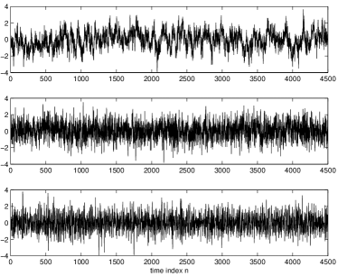
Figure 3: The three source signals used in the simulations.

Here we only provide some preliminary simulation results based on the dual-linear predictor structure [15]. Three source signals are used which are generated by passing three randomly generated white Gaussian signals through three different filters. The power of the sources is normalised to one. The correlation value of each of the source signals is checked to make sure it is positive and not close to zero for one sample shift. Fig. 3 shows the three source signals, denoted by $s_{0}$, $s_{1}$ and $s_{2}$, respectively.

The coefficients of the first linear predictor coefficients ${\bf b}$ were randomly generated with a length of $P=5$, and given by

$${\bf b}=[-0.4548\;-1.0053\;1.1957\;-0.5590\;-0.3617]\;.$$ (53)

For the second linear predictor, $P_{d}=1$, $d_{1}=1$, and $a_{c}=2$.

The normalised correlation value $\hat{r}_{l}$ for each source signal with this dual-linear predictor configuration is $0.0395$, $0.2174$ and $0.7949$, respectively. As already proved, since the first source signal has the smallest correlation value of $0.0395$, it will be extracted by minimizing the cost function.

The $3\times 3$ mixing matrix ${\bf A}$ is randomly generated and given by

$${\bf A}=\left[\begin{array}[]{ccc}0.9207&0.0299&0.3891\\ 0.5165&0.3676&0.7733\\ 0.7822&-0.2735&-0.5598\end{array}\right]\;.$$ (54)

Its row vector is normalised to unity to make sure it is comparable to the noise variance, which is $\sigma_{v}^{2}=0.09$. The forgetting factors is $\beta_{e}=\beta_{y}=\beta_{f}=0.975$ and the stepsize $\mu=0.0015$. A learning curve for this case is shown in Fig. 4, with the performance index defined as [2]

$$PI=10\log_{10}\left(\frac{1}{L-1}(\sum_{l=0}^{L-1}\frac{g_{l}^{2}}{\max\{g_{0}^{2},\dots,g_{L-1}^{2}\}}-1)\right),$$ (55)

with ${\bf g}=[g_{0}\;g_{1}\;\cdots\;g_{L-1}]$.

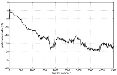
Figure 4: One of the learning curves obtained in our simulations.

To show its performance in a more general context, we change the initial value of the demixing vector ${\bf w}$ randomly each time to run the algorithm and the average learning curve over $1000$ runs is given in Fig. 5. Both curves show a successful extraction of the source signal.

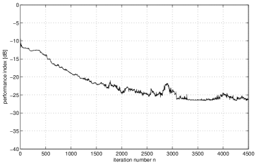
Figure 5: The averaged learning curve over $1000$ runs.

V CONCLUSIONS

The traditional canonical correlation analysis has been generalised to include noisy signals where the effect of noise can be eliminated effectively by the proposed approach. It was then applied to the blind source separation problem and adaptive implementations were derived. In particular, a dual-linear predictor structure was proposed to blindly extract the source signals from their noisy mixtures, and it can be considered as an indirect implementation of GCCA. Some preliminary simulation results have been provided to show the effectiveness of the proposed approach.

References

• [1] A. Hyvarinen, J. Karhunen, and E. Oja, Independent Component Analysis, John Wiley & Sons, Inc., New York, 2001.
• [2] A. Cichocki and S. Amari, Adaptive Blind Signal and Image Processing, John Wiley & Sons, Inc., New York, 2003.
• [3] S.V. Schell and W.A. Gardner, “Programmable canonical correlation analysis: a flexible framework for blind adaptive spatial filtering,” IEEE Transactions on Signal Processing, vol. 42, no. 12, pp. 2898–2908, December 1995.
• [4] J. Galy and C. Adnet, “Canonical correlation analysis: a blind source separation using non-circularity,” in IEEE Workshop on Neural Networks for Signal Processing, Australia, December 2000, vol. 1, pp. 465–473.
• [5] M. Borga and H. Knutsson, “A canonical correlation approach to blind source separation,” Technical report LiU-IMT-EX-0062, Department of Biomedical Engineering, Linkoping University, Sweden, June 2001.
• [6] O. Friman, M. Borga, P. Lundberg, and H. Knutsson, “Exploratory fMRI analysis by autocorrelation maximization,” NeuroImage, vol. 16, pp. 454–464, June 2002.
• [7] W. Liu, D. P. Mandic, and A. Cichocki, “An analysis of the CCA approach for blind source separation and its adaptive realization,” in Proc. IEEE International Symposium on Circuits and Systems, Kos, Greece, May 2006, pp. 3590–3593.
• [8] W. Liu, D. P. Mandic, and A. Cichocki, “Analysis and online realization of the CCA approach for blind source separation,” IEEE Transactions on Neural Networks, vol. 18, no. 5, pp. 1505–1510, September 2007.
• [9] Y. O. Li, T. Adalı, W. Wang, and V. D. Calhoun, “Joint blind source separation by multi-set canonical correlation analysis,” IEEE Transactions on Signal Processing, vol. 57, no. 10, pp. 3918–3929, October 2009.
• [10] B. Peng, W. Liu, and D. P. Mandic, “Subband-based joint blind source separation for convolutive mixtures employing M-CCA,” in Proc. the Constantinides International Workshop on Signal Processing, January 2013.
• [11] B. Peng, W. Liu, and D. P. Mandic, “Design of oversampled generalized discrete fourier transform filter banks for application to subband based blind source separation,” IET Signal Processing, pp. 843–853, December 2013.
• [12] C. Chang, Z. Ding, S. Yau, and F. Chan, “A matrix-pencil approach to blind separation of nonwhite signals in white noise,” in Proc. IEEE International Conference on Acoustics, Speech, and Signal Processing, Seattle, USA, May 1998, vol. 4, pp. 2485–2488.
• [13] W. Liu and D. P. Mandic, “A normalised kurtosis based algorithm for blind source extraction from noisy measurements,” Signal Processing, vol. 86, pp. 1580–1585, July 2006.
• [14] W. Liu, D. P. Mandic, and A. Cichocki, “Blind second-order source extraction of instantaneous noisy mixtures,” IEEE Trans. Circuits and Systems II: Express Briefs, vol. 53, no. 9, pp. 931–935, September 2006.
• [15] W. Liu, D. P. Mandic, and A. Cichocki, “A dual-linear predictor approach to blind source extraction for noisy mixtures,” in Proc. IEEE Workshop on Sensor Array and Multichannel Signal Processing, Darmstadt, Germany, July 2008, pp. 515–519.
• [16] W. Liu, D. P. Mandic, and A. Cichocki, “Blind source separation based on generalised canonical correlation analysis and its adaptive realization,” in Proc. International Congress on Image and Signal Processing, Hainan, China, May 2008, vol. 5, pp. 417–421.
• [17] T. W. Anderson, An Introduction to Multivariate statistical Analysis, John Wiley & Sons, New York, 2rd edition, 1984.
• [18] S. Haykin, Adaptive Filter Theory, Prentice Hall, Englewood Cliffs, New York, 3rd edition, 1996.
• [19] W. Liu, D. P. Mandic, and A. Cichocki, “A class of novel blind source extraction algorithms based on a linear predictor,” in Proc. IEEE International Symposium on Circuits and Systems, Kobe, Japan, May 2005, pp. 3599–3602.
• [20] W. Liu, D. P. Mandic, and A. Cichocki, “Blind source extraction of instantaneous noisy mixtures using a linear predictor,” in Proc. IEEE International Symposium on Circuits and Systems, Kos, Greece, May 2006, pp. 4199–4202.
• [21] W. Liu, D. P. Mandic, and A. Cichocki, “Blind source extraction based on a linear predictor,” IET Signal Processing, vol. 1, no. 1, pp. 29–34, March 2007.
• [22] W. Y. Leong, W. Liu, and D. P. Mandic, “Blind source extraction: standard approaches and extensions to noisy and post-nonlinear mixing,” Neurocomputing, vol. 71, no. 10-12, pp. 2344–2355, June 2008.