Era of Big Data Processing: A New Approach via Tensor Networks and Tensor Decompositions

Andrzej CICHOCKI
RIKEN Brain Science Institute, Japan
and Systems Research Institute of the Polish Academy of Science, Poland
a.cichocki@riken.jp
Part of this work was presented on the International Workshop on Smart Info-Media Systems in Asia, (invited talk - SISA-2013) Sept.30–Oct.2, 2013, Nagoya, Japan
Abstract

Many problems in computational neuroscience, neuroinformatics, pattern/image recognition, signal processing and machine learning generate massive amounts of multidimensional data with multiple aspects and high dimensionality. Tensors (i.e., multi-way arrays) provide often a natural and compact representation for such massive multidimensional data via suitable low-rank approximations. Big data analytics require novel technologies to efficiently process huge datasets within tolerable elapsed times. Such a new emerging technology for multidimensional big data is a multiway analysis via tensor networks (TNs) and tensor decompositions (TDs) which represent tensors by sets of factor (component) matrices and lower-order (core) tensors. Dynamic tensor analysis allows us to discover meaningful hidden structures of complex data and to perform generalizations by capturing multi-linear and multi-aspect relationships. We will discuss some fundamental TN models, their mathematical and graphical descriptions and associated learning algorithms for large-scale TDs and TNs, with many potential applications including: Anomaly detection, feature extraction, classification, cluster analysis, data fusion and integration, pattern recognition, predictive modeling, regression, time series analysis and multiway component analysis.

Keywords: Large-scale HOSVD, Tensor decompositions, CPD, Tucker models, Hierarchical Tucker (HT) decomposition, low-rank tensor approximations (LRA), Tensorization/Quantization, tensor train (TT/QTT) - Matrix Product States (MPS), Matrix Product Operator (MPO), DMRG, Strong Kronecker Product (SKP).

I Introduction and Motivations

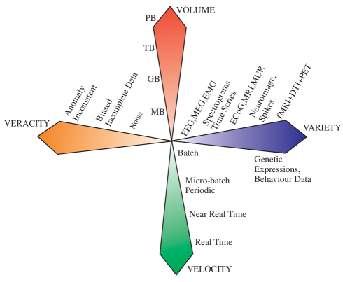
Big Data consists of multidimensional, multi-modal data-sets that are so huge and complex that they cannot be easily stored or processed by using standard computers. Big data are characterized not only by big Volume but also another specific “V” features (see Fig. 1). High Volume implies the need for algorithms that are scalable; High Velocity address the challenges related to process data in near real-time, or virtually real-time; High Veracity demands robust and predictive algorithms for noisy, incomplete or inconsistent data, and finally, high Variety may require integration across different kind of data, e.g., neuroimages, time series, spiking trains, genetic and behavior data.
Refer to caption
Figure  1: Big Data analysis for neuroscience recordings. Brain data can be recorded by electroencephalography (EEG), electrocorticography (ECoG), magnetoencephalography (MEG), fMRI, DTI, PET, Multi Unit Recording (MUR). This involves analysis of multiple modalities/multiple subjects neuroimages, spectrograms, time series, genetic and behavior data. One of the challenges in computational and system neuroscience is to make fusion (assimilation) of such data and to understand the multiple relationships among them in such tasks as perception, cognition and social interactions. The our “V”s of big data: Volume - scale of data, Variety - different forms of data, Veracity - uncertainty of data, and Velocity - analysis of streaming data, comprise the challenges ahead of us.

Many challenging problems for big data are related to capture, manage, search, visualize, cluster, classify, assimilate, merge, and process the data within a tolerable elapsed time, hence demanding new innovative solutions and technologies. Such emerging technology is Tensor Decompositions (TDs) and Tensor Networks (TNs) via low-rank matrix/tensor approximations. The challenge is how to analyze large-scale, multiway data sets. Data explosion creates deep research challenges that require new scalable, TD and TN algorithms.
Refer to caption
Refer to caption
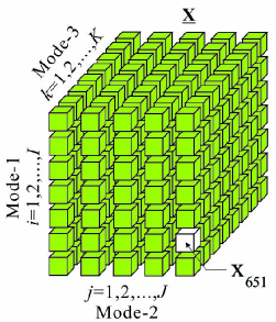
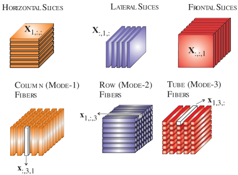
Figure  2: A 3rd-order tensor 𝐗¯I×J×K¯𝐗superscript𝐼𝐽𝐾\underline{{\bf X}}\in\mathbb{R}^{I\times J\times K}, with entries xi,j,k=𝐗¯(i,j,k)subscript𝑥𝑖𝑗𝑘¯𝐗𝑖𝑗𝑘x_{i,j,k}=\underline{{\bf X}}(i,j,k) and its sub-tensors: Slices and fibers. All fibers are treated as column vectors.

(a)

Refer to caption

(b)

Refer to caption
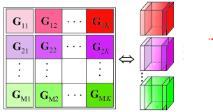
Figure  3: Block matrices and their representations by (a) a 3rd-order tensor and (b) a 4th-order tensor.

Tensors are adopted in diverse branches of science such as a data analysis, signal and image processing [1, 2, 3, 4], Psychometric, Chemometrics, Biometric, Quantum Physics/Information, and Quantum Chemistry [5, 6, 7]. Modern scientific areas such as bioinformatics or computational neuroscience generate massive amounts of data collected in various forms of large-scale, sparse tabular, graphs or networks with multiple aspects and high dimensionality.

Tensors, which are multi-dimensional generalizations of matrices (see Fig. 2 and Fig. 3), provide often a useful representation for such data. Tensor decompositions (TDs) decompose data tensors in factor matrices, while tensor networks (TNs) represent higher-order tensors by interconnected lower-order tensors. We show that TDs and TNs provide natural extensions of blind source separation (BSS) and 2-way (matrix) Component Analysis (2-way CA) to multi-way component analysis (MWCA) methods. In addition, TD and TN algorithms are suitable for dimensionality reduction and they can handle missing values, and noisy data. Moreover, they are potentially useful for analysis of linked (coupled) block of tensors with millions and even billions of non-zero entries, using the map-reduce paradigm, as well as divide-and-conquer approaches [8, 9, 10]. This all suggest that multidimensional data can be represented by linked multi-block tensors which can be decomposed into common (or correlated) and distinctive (uncorrelated, indpendent) components [3, 11, 12]. Effective analysis of coupled tensors requires the development of new models and associated algorithms that can identify the core relations that exist among the different tensor modes, and the same tome scale to extremely large datasets. Our objective is to develop suitable models and algorithms for linked low-rank tensor approximations (TAs), and associated scalable software to make such analysis possible.

Review and tutorial papers [2, 4, 13, 14, 15] and books [6, 5, 1] dealing with TDs already exist, however, they typically focus on standard TDs and/or do not provide explicit links to big data processing topics and do not explore natural connections with emerging areas including multi-block coupled tensor analysis and tensor networks. This paper extends beyond the standard TD models and aims to elucidate the power and flexibility of TNs in the analysis of multi-dimensional, multi-modal, and multi-block data, together with their role as a mathematical backbone for the discovery of hidden structures in large-scale data [1, 2, 4].

Motivations - Why low-rank tensor approximations? A wealth of literature on (2-way) component analysis (CA) and BSS exists, especially on Principal Component Analysis (PCA), Independent Component Analysis (ICA), Sparse Component Analysis (SCA), Nonnegative Matrix Factorizations (NMF), and Morphological Component Analysis (MCA) [16, 1, 17]. These techniques are maturing, and are promising tools for blind source separation (BSS), dimensionality reduction, feature extraction, clustering, classification, and visualization [1, 17].

The “flattened view” provided by 2-way CA and matrix factorizations (PCA/SVD, NMF, SCA, MCA) may be inappropriate for large classes of real-world data which exhibit multiple couplings and cross-correlations. In this context, higher-order tensor networks give us the opportunity to develop more sophisticated models performing distributed computing and capturing multiple interactions and couplings, instead of standard pairwise interactions. In other words, to discover hidden components within multiway data the analysis tools should account for intrinsic multi-dimensional distributed patterns present in the data.
Refer to caption
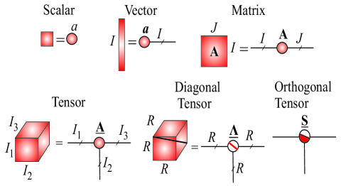
Figure  4: Basic symbols for tensor network diagrams.

II Basic Tensor Operations

TABLE I: Basic tensor notation and symbols. A tensor are denoted by underline bold capital letters, matrices by uppercase bold letters, vectors by lowercase boldface letters and scalars by lowercase letters.

𝐗¯I1×I2××IN¯𝐗superscriptsubscript𝐼1subscript𝐼2subscript𝐼𝑁\underline{{\bf X}}\in\mathbb{R}^{I_{1}\times I_{2}\times\cdots\times I_{N}} N𝑁Nth-order tensor of size I1×I2××INsubscript𝐼1subscript𝐼2subscript𝐼𝑁I_{1}\times I_{2}\times\cdots\times I_{N} 𝐆¯,𝐆¯r,𝐆¯𝐗,𝐆¯𝐘,𝐒¯¯𝐆subscript¯𝐆𝑟subscript¯𝐆𝐗subscript¯𝐆𝐘¯𝐒\underline{{\bf G}},\;\underline{{\bf G}}_{r},\;\underline{{\bf G}}_{{\bf X}},\;\underline{{\bf G}}_{{\bf Y}},\;\underline{{\bf S}} core tensors 𝚲¯R×R××R¯𝚲superscript𝑅𝑅𝑅\underline{\mbox{\boldmath$\Lambda$}}\in\mathbb{R}^{R\times R\times\cdots\times R} N𝑁Nth-order diagonal core tensor with nonzero λrsubscript𝜆𝑟\lambda_{r} entries on main diagonal 𝐀=[𝒂1,𝒂2,,𝒂R]I×R𝐀subscript𝒂1subscript𝒂2subscript𝒂𝑅superscript𝐼𝑅{\bf A}=[\mbox{\boldmath$a$}_{1},\mbox{\boldmath$a$}_{2},\ldots,\mbox{\boldmath$a$}_{R}]\in\mathbb{R}^{I\times R} matrix with column vectors 𝒂rIsubscript𝒂𝑟superscript𝐼\mbox{\boldmath$a$}_{r}\in\mathbb{R}^{I} and entries airsubscript𝑎𝑖𝑟a_{ir} 𝐀,𝐁,𝐂,𝐁(n),𝐔(n)𝐀𝐁𝐂superscript𝐁𝑛superscript𝐔𝑛{\bf A},\,{\bf B},\,{\bf C},\;{\bf B}^{(n)},\;{\bf U}^{(n)} component matrices 𝒊=[i1,i2,,iN]𝒊subscript𝑖1subscript𝑖2subscript𝑖𝑁\mbox{\boldmath$i$}=[i_{1},i_{2},\ldots,i_{N}] vector of indices 𝐗(n)In×I1In1In+1INsubscript𝐗𝑛superscriptsubscript𝐼𝑛subscript𝐼1subscript𝐼𝑛1subscript𝐼𝑛1subscript𝐼𝑁{\bf X}_{(n)}\in\mathbb{R}^{I_{n}\times I_{1}\cdots I_{n-1}I_{n+1}\cdots I_{N}} mode-n𝑛n unfolding of 𝐗¯¯𝐗\underline{{\bf X}} 𝒙:,i2,i3,,iNsubscript𝒙:subscript𝑖2subscript𝑖3subscript𝑖𝑁\mbox{\boldmath$x$}_{:,i_{2},i_{3},\ldots,i_{N}} mode-1 fiber of 𝐗¯¯𝐗\underline{{\bf X}} obtained by fixing all but one index 𝐗:,:,i3,,iNsubscript𝐗::subscript𝑖3subscript𝑖𝑁{\bf X}_{:,:,i_{3},\ldots,i_{N}} tensor slice of 𝐗¯¯𝐗\underline{{\bf X}} obtained by fixing all but two indices 𝐗¯:,:,:,i4,,iNsubscript¯𝐗:::subscript𝑖4subscript𝑖𝑁\underline{{\bf X}}_{:,:,:,i_{4},\ldots,i_{N}} subtensor of 𝐗¯¯𝐗\underline{{\bf X}}, in which several indices are fixed 𝒙=vec(𝐗¯)𝒙vec¯𝐗\mbox{\boldmath$x$}=\operatorname{vec}\left(\underline{{\bf X}}\right) vectorization of 𝐗¯¯𝐗\underline{{\bf X}} diag{}diag\mathop{\rm diag}\nolimits\{\bullet\} diagonal matrix

(a)

Refer to caption

(b)

Refer to caption

(c)

Refer to caption
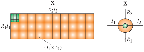
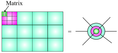
Figure  5: Hierarchical block matrices and their representations as tensors: (a) a 4th-order tensor for a block matrix 𝐗R1I1×R2I2𝐗superscriptsubscript𝑅1subscript𝐼1subscript𝑅2subscript𝐼2{\bf X}\in\mathbb{R}^{R_{1}I_{1}\times R_{2}I_{2}}, comprising block matrices 𝐗r1,r2I1×I2subscript𝐗subscript𝑟1subscript𝑟2superscriptsubscript𝐼1subscript𝐼2{\bf X}_{r_{1},r_{2}}\in\mathbb{R}^{I_{1}\times I_{2}}, (b) a 5th-order tensor and (c) a 6th-order tensor.
Refer to caption

4th-order tensor
Refer to captionRefer to caption
5th-order tensors
Refer to caption
6th-order tensor

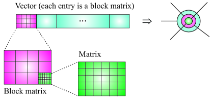
Figure  6: Graphical representations and symbols for higher-order block tensors. Each block represents a 3rd-order tensor or 2nd-order tensor. An external circle represent a global structure of the block tensor (e.g., a vector, a matrix, a 3rd-order tensor) and inner circle represents a structure of each element of the block tensor.

(a)
Refer to caption
(b)
Refer to caption

Figure  7: Unfoldings in tensor networks: (a) Graphical representation of the basic mode-n𝑛n unfolding (matricization, flattening) 𝐀(n)In×I1In1In+1INsubscript𝐀𝑛superscriptsubscript𝐼𝑛subscript𝐼1subscript𝐼𝑛1subscript𝐼𝑛1subscript𝐼𝑁{\bf A}_{(n)}\in\mathbb{R}^{I_{n}\times I_{1}\cdots I_{n-1}I_{n+1}\cdots I_{N}} for an N𝑁Nth-order tensor 𝐀¯I1×I2××IN¯𝐀superscriptsubscript𝐼1subscript𝐼2subscript𝐼𝑁\underline{{\bf A}}\in\mathbb{R}^{I_{1}\times I_{2}\times\cdots\times I_{N}}. (b) More general unfolding of the N𝑁Nth-order tensor into a matrix 𝐀([n])=𝐀(i1,,in¯;in+1,,iN¯)I1I2In×In+1INsubscript𝐀delimited-[]𝑛subscript𝐀¯subscript𝑖1subscript𝑖𝑛¯subscript𝑖𝑛1subscript𝑖𝑁superscriptsubscript𝐼1subscript𝐼2subscript𝐼𝑛subscript𝐼𝑛1subscript𝐼𝑁{\bf A}_{([n])}={\bf A}_{(\overline{i_{1},\ldots,i_{n}}\;;\;\overline{i_{n+1},\ldots,i_{N}})}\in\mathbb{R}^{I_{1}I_{2}\cdots I_{n}\times I_{n+1}\cdots I_{N}}. All entries of an unfolded tensor are arranged in a specific order, e.g., in lexicographical order. In a more general case, let 𝒓={m1,m2,,mR}{1,2,,N}𝒓subscript𝑚1subscript𝑚2subscript𝑚𝑅12𝑁\mbox{\boldmath$r$}=\{m_{1},m_{2},\ldots,m_{R}\}\subset\{1,2,\ldots,N\} be the row indices and 𝒄={n1,n2,,nC}{1,2,,N}𝒓𝒄subscript𝑛1subscript𝑛2subscript𝑛𝐶12𝑁𝒓\mbox{\boldmath$c$}=\{n_{1},n_{2},\ldots,n_{C}\}\subset\{1,2,\ldots,N\}-\mbox{\boldmath$r$} be the column indices, then the mode-(𝒓,𝒄)𝒓𝒄(\mbox{\boldmath$r$},\mbox{\boldmath$c$}) unfolding of 𝐀¯¯𝐀\underline{{\bf A}} is denoted as 𝐀(𝒓,𝒄)Im1Im2ImR×In1In2InCsubscript𝐀𝒓𝒄superscriptsubscript𝐼subscript𝑚1subscript𝐼subscript𝑚2subscript𝐼subscript𝑚𝑅subscript𝐼subscript𝑛1subscript𝐼subscript𝑛2subscript𝐼subscript𝑛𝐶{\bf A}_{(\mbox{\boldmath$r$},\mbox{\boldmath$c$})}\in\mathbb{R}^{I_{m_{1}}I_{m_{2}}\cdots I_{m_{R}}\times I_{n_{1}}I_{n_{2}}\cdots I_{n_{C}}}.
TABLE II: Basic tensor/matrix operations.

𝐂¯=𝐀¯×n𝐁¯𝐂subscript𝑛¯𝐀𝐁\underline{{\bf C}}=\underline{{\bf A}}\times_{n}{\bf B} mode-n𝑛n product of 𝐀¯I1×I2××IN¯𝐀superscriptsubscript𝐼1subscript𝐼2subscript𝐼𝑁\underline{{\bf A}}\in\mathbb{R}^{I_{1}\times I_{2}\times\cdots\times I_{N}} and 𝐁Jn×In𝐁superscriptsubscript𝐽𝑛subscript𝐼𝑛{\bf B}\in\mathbb{R}^{J_{n}\times I_{n}} yields 𝐂¯I1××In1×Jn×In+1××IN¯𝐂superscriptsubscript𝐼1subscript𝐼𝑛1subscript𝐽𝑛subscript𝐼𝑛1subscript𝐼𝑁\underline{{\bf C}}\in\mathbb{R}^{I_{1}\times\cdots\times I_{n-1}\times J_{n}\times I_{n+1}\times\cdots\times I_{N}}, with entries ci1,,in1,j,in+1,iN=in=1Inai1,,in,,iNbj,insubscript𝑐subscript𝑖1subscript𝑖𝑛1𝑗subscript𝑖𝑛1subscript𝑖𝑁superscriptsubscriptsubscript𝑖𝑛1subscript𝐼𝑛subscript𝑎subscript𝑖1subscript𝑖𝑛subscript𝑖𝑁subscript𝑏𝑗subscript𝑖𝑛c_{i_{1},\ldots,i_{n-1},\,j,\,i_{n+1},\ldots i_{N}}=\sum_{i_{n}=1}^{I_{n}}a_{i_{1},\ldots,i_{n},\ldots,i_{N}}b_{j,\,i_{n}}, or equivalently 𝐂(n)=𝐁𝐀(n)subscript𝐂𝑛𝐁subscript𝐀𝑛{\bf C}_{(n)}={\bf B}\,{\bf A}_{(n)} 𝐂¯=𝐀¯;𝐁(1),,𝐁(N)=𝐀¯×1𝐁(1)×2𝐁(2)×N𝐁(N)¯𝐂¯𝐀superscript𝐁1superscript𝐁𝑁subscript𝑁subscript2subscript1¯𝐀superscript𝐁1superscript𝐁2superscript𝐁𝑁\underline{{\bf C}}=\llbracket\underline{{\bf A}};{\bf B}^{(1)},\ldots,{\bf B}^{(N)}\rrbracket=\underline{{\bf A}}\times_{1}{\bf B}^{(1)}\times_{2}{\bf B}^{(2)}\cdots\times_{N}{\bf B}^{(N)} 𝐂¯=𝐀¯𝐁¯¯𝐂¯𝐀¯𝐁\underline{{\bf C}}=\underline{{\bf A}}\circ\underline{{\bf B}} tensor or outer product of 𝐀¯I1×I2××IN¯𝐀superscriptsubscript𝐼1subscript𝐼2subscript𝐼𝑁\underline{{\bf A}}\in\mathbb{R}^{I_{1}\times I_{2}\times\cdots\times I_{N}} and 𝐁¯J1×J2××JM¯𝐁superscriptsubscript𝐽1subscript𝐽2subscript𝐽𝑀\underline{{\bf B}}\in\mathbb{R}^{J_{1}\times J_{2}\times\cdots\times J_{M}} yields (N+M)𝑁𝑀(N+M)th-order tensor 𝐂¯¯𝐂\underline{{\bf C}}, with entries ci1,,iN,j1,,jM=ai1,,iNbj1,,jMsubscript𝑐subscript𝑖1subscript𝑖𝑁subscript𝑗1subscript𝑗𝑀subscript𝑎subscript𝑖1subscript𝑖𝑁subscript𝑏subscript𝑗1subscript𝑗𝑀c_{i_{1},\ldots,i_{N},\,j_{1},\ldots,j_{M}}=a_{i_{1},\ldots,i_{N}}b_{j_{1},\ldots,j_{M}} 𝐗¯=𝒂𝒃𝒄I×J×K¯𝐗𝒂𝒃𝒄superscript𝐼𝐽𝐾\underline{{\bf X}}=\mbox{\boldmath$a$}\circ\mbox{\boldmath$b$}\circ\mbox{\boldmath$c$}\in\mathbb{R}^{I\times J\times K} tensor or outer product of vectors forms a rank-1 tensor, with entries xijk=aibjcksubscript𝑥𝑖𝑗𝑘subscript𝑎𝑖subscript𝑏𝑗subscript𝑐𝑘x_{ijk}=a_{i}b_{j}c_{k} 𝐀Tsuperscript𝐀𝑇{{\bf A}}^{T}, 𝐀1superscript𝐀1{{\bf A}}^{-1}, 𝐀superscript𝐀{{\bf A}}^{{\dagger}} transpose, inverse and Moore-Penrose pseudo-inverse of 𝐀𝐀{\bf A} 𝐂¯=𝐀¯𝐁¯¯𝐂tensor-product¯𝐀¯𝐁\underline{{\bf C}}=\underline{{\bf A}}\otimes\underline{{\bf B}} Kronecker product of 𝐀¯I1×I2××IN¯𝐀superscriptsubscript𝐼1subscript𝐼2subscript𝐼𝑁\underline{{\bf A}}\in\mathbb{R}^{I_{1}\times I_{2}\times\cdots\times I_{N}} and 𝐁¯J1×J2××JN¯𝐁superscriptsubscript𝐽1subscript𝐽2subscript𝐽𝑁\underline{{\bf B}}\in\mathbb{R}^{J_{1}\times J_{2}\times\cdots\times J_{N}} yields 𝐂¯I1J1××INJN¯𝐂superscriptsubscript𝐼1subscript𝐽1subscript𝐼𝑁subscript𝐽𝑁\underline{{\bf C}}\in\mathbb{R}^{I_{1}J_{1}\times\cdots\times I_{N}J_{N}}, with entries ci1,j1¯,,iN,jN¯=ai1,,iNbj1,,jNsubscript𝑐¯subscript𝑖1subscript𝑗1¯subscript𝑖𝑁subscript𝑗𝑁subscript𝑎subscript𝑖1subscript𝑖𝑁subscript𝑏subscript𝑗1subscript𝑗𝑁c_{\overline{i_{1},j_{1}},\ldots,\overline{i_{N},j_{N}}}=a_{i_{1},\ldots,i_{N}}\>b_{j_{1},\ldots,j_{N}}, where in,jn¯=jn+(in1)Jn¯subscript𝑖𝑛subscript𝑗𝑛subscript𝑗𝑛subscript𝑖𝑛1subscript𝐽𝑛\overline{i_{n},j_{n}}=j_{n}+(i_{n}-1)J_{n} 𝐂=𝐀𝐁𝐂direct-product𝐀𝐁{\bf C}={\bf A}\odot{\bf B} Khatri-Rao product of 𝐀I×J𝐀superscript𝐼𝐽{\bf A}\in\mathbb{R}^{I\times J} and 𝐁K×J𝐁superscript𝐾𝐽{\bf B}\in\mathbb{R}^{K\times J} yields 𝐂IK×J𝐂superscript𝐼𝐾𝐽{\bf C}\in\mathbb{R}^{IK\times J}, with columns 𝒄j=𝒂j𝒃jsubscript𝒄𝑗tensor-productsubscript𝒂𝑗subscript𝒃𝑗\mbox{\boldmath$c$}_{j}=\mbox{\boldmath$a$}_{j}\otimes\mbox{\boldmath$b$}_{j}

A higher-order tensor can be interpreted as a multiway array, as illustrated graphically in Figs. 2, 3 and 4. Our adopted convenience is that tensors are denoted by bold underlined capital letters, e.g., 𝐗¯I1×I2××IN¯𝐗superscriptsubscript𝐼1subscript𝐼2subscript𝐼𝑁\underline{{\bf X}}\in\mathbb{R}^{I_{1}\times I_{2}\times\cdots\times I_{N}}, and that all data are real-valued. The order of a tensor is the number of its “modes”, “ways” or “dimensions”, which can include space, time, frequency, trials, classes, and dictionaries. Matrices (2nd-order tensors) are denoted by boldface capital letters, e.g., 𝐗𝐗{\bf X}, and vectors (1st-order tensors) by boldface lowercase letters; for instance the columns of the matrix 𝐀=[𝒂1,𝒂2,,𝒂R]I×R𝐀subscript𝒂1subscript𝒂2subscript𝒂𝑅superscript𝐼𝑅{\bf A}=[\mbox{\boldmath$a$}_{1},\mbox{\boldmath$a$}_{2},\ldots,\mbox{\boldmath$a$}_{R}]\in\mathbb{R}^{I\times R} are denoted by 𝒂rsubscript𝒂𝑟\mbox{\boldmath$a$}_{r} and elements of a matrix (scalars) are denoted by lowercase letters, e.g., airsubscript𝑎𝑖𝑟a_{ir} (see Table I).

The most common types of tensor multiplications are denoted by: tensor-product\otimes for the Kronecker, direct-product\odot for the Khatri-Rao, \circledast for the Hadamard (componentwise), \circ for the outer and ×nsubscript𝑛\times_{n} for the mode-n𝑛n products (see Table II).

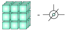
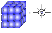
TNs and TDs can be represented by tensor network diagrams, in which tensors are represented graphically by nodes or any shapes (e.g., circles, spheres, triangular, squares, ellipses) and each outgoing edge (line) emerging from a shape represents a mode (a way, dimension, indices) (see Fig. 4) Tensor network diagrams are very useful not only in visualizing tensor decompositions, but also in their different transformations/reshapings and graphical illustrations of mathematical (multilinear) operations.

It should also be noted that block matrices and hierarchical block matrices can be represented by tensors. For example, 3rd-order and 4th-order tensors that can be represented by block matrices as illustrated in Fig. 3 and all algebraic operations can be performed on block matrices. Analogously, higher-order tensors can be represented as illustrated in Fig. 5 and Fig. 6. Subtensors are formed when a subset of indices is fixed. Of particular interest are fibers, defined by fixing every index but one, and matrix slices which are two-dimensional sections (matrices) of a tensor, obtained by fixing all the indices but two (see Fig. 2). A matrix has two modes: rows and columns, while an N𝑁Nth-order tensor has N𝑁N modes.

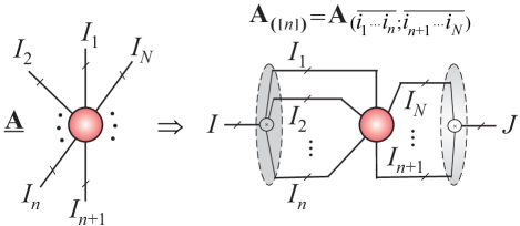
The process of unfolding (see Fig. 7) flattens a tensor into a matrix. In the simplest scenario, mode-n𝑛n unfolding (matricization, flattening) of the tensor 𝐀¯I1×I2××IN¯𝐀superscriptsubscript𝐼1subscript𝐼2subscript𝐼𝑁\underline{{\bf A}}\in\mathbb{R}^{I_{1}\times I_{2}\times\cdots\times I_{N}} yields a matrix 𝐀(n)In×(I1In1In+1IN)subscript𝐀𝑛superscriptsubscript𝐼𝑛subscript𝐼1subscript𝐼𝑛1subscript𝐼𝑛1subscript𝐼𝑁{\bf A}_{(n)}\in\mathbb{R}^{I_{n}\times(I_{1}\cdots I_{n-1}I_{n+1}\cdots I_{N})}, with entries ain,(j1,,in1,jn+1,,in)subscript𝑎subscript𝑖𝑛subscript𝑗1subscript𝑖𝑛1subscript𝑗𝑛1subscript𝑖𝑛a_{i_{n},(j_{1},\ldots,i_{n-1},j_{n+1},\ldots,i_{n})} such that remaining indices (i1,,in1,in+1,,iN)subscript𝑖1subscript𝑖𝑛1subscript𝑖𝑛1subscript𝑖𝑁(i_{1},\ldots,i_{n-1},i_{n+1},\ldots,i_{N}) are arranged in a specific order, e.g., in the lexicographical order [4]. In tensor networks we use, typically a generalized mode-([n])delimited-[]𝑛([n]) unfolding as illustrated in Fig. 7 (b).

By a multi-index i=i1,i2,,iN¯𝑖¯subscript𝑖1subscript𝑖2subscript𝑖𝑁i=\overline{i_{1},i_{2},\ldots,i_{N}}, we denote an index which takes all possible combinations of values of i1,i2,,insubscript𝑖1subscript𝑖2subscript𝑖𝑛i_{1},i_{2},\ldots,i_{n}, for in=1,2,,Insubscript𝑖𝑛12subscript𝐼𝑛i_{n}=1,2,\ldots,I_{n} in a specific and consistent orders. The entries of matrices or tensors in matricized and/or vectorized forms can be ordered in at least two different ways.

Remark: The multi–index can be defined using two different conventions:

1) The little -endian convention

i1,i2,,iN¯¯subscript𝑖1subscript𝑖2subscript𝑖𝑁\displaystyle\overline{i_{1},i_{2},\ldots,i_{N}} =\displaystyle= i1+(i21)I1+(i31)I1I2subscript𝑖1subscript𝑖21subscript𝐼1subscript𝑖31subscript𝐼1subscript𝐼2\displaystyle i_{1}+(i_{2}-1)I_{1}+(i_{3}-1)I_{1}I_{2} (1)
\displaystyle\cdots +(iN1)I1IN1.subscript𝑖𝑁1subscript𝐼1subscript𝐼𝑁1\displaystyle+(i_{N}-1)I_{1}\cdots I_{N-1}.

2) The big -endian

i1,i2,,iN¯=iN+(iN11)IN+¯subscript𝑖1subscript𝑖2subscript𝑖𝑁subscript𝑖𝑁limit-fromsubscript𝑖𝑁11subscript𝐼𝑁\displaystyle\overline{i_{1},i_{2},\ldots,i_{N}}=i_{N}+(i_{N-1}-1)I_{N}+
+(iN21)ININ1++(i11)I2IN.subscript𝑖𝑁21subscript𝐼𝑁subscript𝐼𝑁1subscript𝑖11subscript𝐼2subscript𝐼𝑁\displaystyle+(i_{N-2}-1)I_{N}I_{N-1}+\cdots+(i_{1}-1)I_{2}\cdots I_{N}. (2)

The little–endian notation is consistent with the Fortran style of indexing, while the big–endian notation is similar to numbers written in the positional system and corresponds to reverse lexicographic order. The definition unfolding of tensors and the Kronecker (tensor) product tensor-product\otimes should be also consistent with the chosen convention111The standard and more popular definition in multilinear algebra assumes the big–endian convention, while for the development of the efficient program code for big data usually the little–endian convention seems to be more convenient (see for more detail papers of Dolgov and Savostyanov [18, 19]).. In this paper we will use the big-endian notation, however it is enough to remember that 𝒄=𝒂𝒃𝒄tensor-product𝒂𝒃\mbox{\boldmath$c$}=\mbox{\boldmath$a$}\otimes\mbox{\boldmath$b$} means that ci,j¯=aibjsubscript𝑐¯𝑖𝑗subscript𝑎𝑖subscript𝑏𝑗c_{\overline{i,j}}=a_{i}b_{j}.

The Kronecker product of two tensors: 𝐀¯I1×I2×IN¯𝐀superscriptsubscript𝐼1subscript𝐼2subscript𝐼𝑁\underline{{\bf A}}\in\mathbb{R}^{I_{1}\times I_{2}\cdots\times I_{N}} and 𝐁¯J1×J2××JN¯𝐁superscriptsubscript𝐽1subscript𝐽2subscript𝐽𝑁\underline{{\bf B}}\in\mathbb{R}^{J_{1}\times J_{2}\times\cdots\times J_{N}} yields 𝐂¯=𝐀¯𝐁¯I1I2××INJN¯𝐂tensor-product¯𝐀¯𝐁superscriptsubscript𝐼1subscript𝐼2subscript𝐼𝑁subscript𝐽𝑁\underline{{\bf C}}=\underline{{\bf A}}\otimes\underline{{\bf B}}\in\mathbb{R}^{I_{1}I_{2}\times\cdots\times I_{N}J_{N}}, with entries ci1,j1¯,,iN,jN¯=ai1,,iNbj1,,jNsubscript𝑐¯subscript𝑖1subscript𝑗1¯subscript𝑖𝑁subscript𝑗𝑁subscript𝑎subscript𝑖1subscript𝑖𝑁subscript𝑏subscript𝑗1subscript𝑗𝑁c_{\overline{i_{1},j_{1}},\ldots,\overline{i_{N},j_{N}}}=a_{i_{1},\ldots,i_{N}}\>b_{j_{1},\ldots,j_{N}}, where in,jn¯=jn+(in1)Jn¯subscript𝑖𝑛subscript𝑗𝑛subscript𝑗𝑛subscript𝑖𝑛1subscript𝐽𝑛\overline{i_{n},j_{n}}=j_{n}+(i_{n}-1)J_{n}.

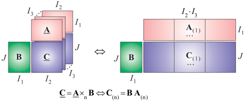
The mode-n𝑛n product of a tensor 𝐀¯I1××IN¯𝐀superscriptsubscript𝐼1subscript𝐼𝑁\underline{{\bf A}}\in\mathbb{R}^{I_{1}\times\cdots\times I_{N}} by a vector 𝒃In𝒃superscriptsubscript𝐼𝑛\mbox{\boldmath$b$}\in\mathbb{R}^{I_{n}} is defined as a tensor 𝐂¯=𝐀¯×¯n𝒃I1××In1×In+1××IN¯𝐂¯𝐀subscript¯𝑛𝒃superscriptsubscript𝐼1subscript𝐼𝑛1subscript𝐼𝑛1subscript𝐼𝑁\underline{{\bf C}}=\underline{{\bf A}}\bar{\times}_{n}\mbox{\boldmath$b$}\in\mathbb{R}^{I_{1}\times\cdots\times I_{n-1}\times I_{n+1}\times\cdots\times I_{N}}, with entries ci1,,in1,in+1,,iN=in=1In(ai1,i2,,iN)binsubscript𝑐subscript𝑖1subscript𝑖𝑛1subscript𝑖𝑛1subscript𝑖𝑁superscriptsubscriptsubscript𝑖𝑛1subscript𝐼𝑛subscript𝑎subscript𝑖1subscript𝑖2subscript𝑖𝑁subscript𝑏subscript𝑖𝑛c_{i_{1},\ldots,i_{n-1},i_{n+1},\ldots,i_{N}}=\sum_{i_{n}=1}^{I_{n}}(a_{i_{1},i_{2},\ldots,i_{N}})\;b_{i_{n}}, while a mode-n𝑛n product of the tensor 𝐀¯I1××IN¯𝐀superscriptsubscript𝐼1subscript𝐼𝑁\underline{{\bf A}}\in\mathbb{R}^{I_{1}\times\cdots\times I_{N}} by a matrix 𝐁J×In𝐁superscript𝐽subscript𝐼𝑛{\bf B}\in\mathbb{R}^{J\times I_{n}} is the tensor 𝐂¯=𝐀¯×n𝐁I1××In1×J×In+1××IN¯𝐂subscript𝑛¯𝐀𝐁superscriptsubscript𝐼1subscript𝐼𝑛1𝐽subscript𝐼𝑛1subscript𝐼𝑁\underline{{\bf C}}=\underline{{\bf A}}\times_{n}{\bf B}\in\mathbb{R}^{I_{1}\times\cdots\times I_{n-1}\times J\times I_{n+1}\times\cdots\times I_{N}}, with entries ci1,i2,,in1,j,in+1,,iN=in=1Inai1,i2,,iNbj,insubscript𝑐subscript𝑖1subscript𝑖2subscript𝑖𝑛1𝑗subscript𝑖𝑛1subscript𝑖𝑁superscriptsubscriptsubscript𝑖𝑛1subscript𝐼𝑛subscript𝑎subscript𝑖1subscript𝑖2subscript𝑖𝑁subscript𝑏𝑗subscript𝑖𝑛c_{i_{1},i_{2},\ldots,i_{n-1},j,i_{n+1},\ldots,i_{N}}=\sum_{i_{n}=1}^{I_{n}}a_{i_{1},i_{2},\ldots,i_{N}}\;b_{j,i_{n}}. This can also be expressed in a matrix form as 𝐂(n)=𝐁𝐀(n)subscript𝐂𝑛subscript𝐁𝐀𝑛{\bf C}_{(n)}={\bf B}{\bf A}_{(n)} (see Fig. 8), which allows us to employ fast matrix by vector and matrix by matrix multiplications for very large scale problems.

(a)
Refer to caption
(b)
Refer to caption

Figure  8: From a matrix format to the tensor network format. (a) Multilinear mode-111 product of a 3rd-order tensor 𝐀¯I1×I2×I3¯𝐀superscriptsubscript𝐼1subscript𝐼2subscript𝐼3\underline{{\bf A}}\in\mathbb{R}^{I_{1}\times I_{2}\times I_{3}} and a factor (component) matrix 𝐁J×I1𝐁superscript𝐽subscript𝐼1{\bf B}\in\mathbb{R}^{J\times I_{1}} yields a tensor 𝐂¯=𝐀¯×1𝐁J×I2×I3¯𝐂subscript1¯𝐀𝐁superscript𝐽subscript𝐼2subscript𝐼3\underline{{\bf C}}=\underline{{\bf A}}\times_{1}{\bf B}\in\mathbb{R}^{J\times I_{2}\times I_{3}}. This is equivalent to simple matrix multiplication formula 𝐂(1)=𝐁𝐀(1)subscript𝐂1subscript𝐁𝐀1{\bf C}_{(1)}={\bf B}{\bf A}_{(1)}. (b) Multilinear mode-n𝑛n product an N𝑁Nth-order tensor and a factor matrix 𝐁J×In𝐁superscript𝐽subscript𝐼𝑛{\bf B}\in\mathbb{R}^{J\times I_{n}}.

If we take all the modes, then we have a full multilinear product of a tensor and a set of matrices, which is compactly written as [4] (see Fig. 9 (a))):

𝐂¯¯𝐂\displaystyle\underline{{\bf C}} =\displaystyle= 𝐆¯×1𝐁(1)×2𝐁(2)×N𝐁(N)subscript𝑁subscript2subscript1¯𝐆superscript𝐁1superscript𝐁2superscript𝐁𝑁\displaystyle\underline{{\bf G}}\times_{1}{\bf B}^{(1)}\times_{2}{\bf B}^{(2)}\cdots\times_{N}{\bf B}^{(N)} (3)
=\displaystyle= 𝐆¯;𝐁(1),𝐁(2),,𝐁(N).¯𝐆superscript𝐁1superscript𝐁2superscript𝐁𝑁\displaystyle\llbracket\underline{{\bf G}};{\bf B}^{(1)},{\bf B}^{(2)},\ldots,{\bf B}^{(N)}\rrbracket.

(a)                                               (b)
Refer to caption

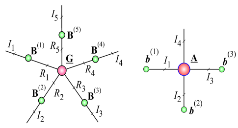
Figure  9: Multilinear products via tensor network diagrams. (a) Multilinear full product of tensor (Tucker decomposition) 𝐆¯R1×R2××R5¯𝐆superscriptsubscript𝑅1subscript𝑅2subscript𝑅5\underline{{\bf G}}\in\mathbb{R}^{R_{1}\times R_{2}\times\cdots\times R_{5}} and factor (component) matrices 𝐁(n)In×Rnsuperscript𝐁𝑛superscriptsubscript𝐼𝑛subscript𝑅𝑛{\bf B}^{(n)}\in\mathbb{R}^{I_{n}\times R_{n}} (n=1,2,,5𝑛125n=1,2,\ldots,5) yields the Tucker tensor decomposition 𝐂¯=𝐆¯×1𝐁(1)×2𝐁(2)×5𝐁(5)I1×I2××I5¯𝐂subscript5subscript2subscript1¯𝐆superscript𝐁1superscript𝐁2superscript𝐁5superscriptsubscript𝐼1subscript𝐼2subscript𝐼5\underline{{\bf C}}=\underline{{\bf G}}\times_{1}{\bf B}^{(1)}\times_{2}{\bf B}^{(2)}\cdots\times_{5}{\bf B}^{(5)}\in\mathbb{R}^{I_{1}\times I_{2}\times\cdots\times I_{5}}. b) Multilinear product of tensor 𝐀¯I1×I2××I4¯𝐀superscriptsubscript𝐼1subscript𝐼2subscript𝐼4\underline{{\bf A}}\in\mathbb{R}^{I_{1}\times I_{2}\times\cdots\times I_{4}} and vectors 𝒃nInsubscript𝒃𝑛superscriptsubscript𝐼𝑛\mbox{\boldmath$b$}_{n}\in\mathbb{R}^{I_{n}} (n=1,2,3)𝑛123(n=1,2,3) yields a vector 𝒄=𝐀¯×¯1𝒃(1)ׯ2𝒃(2)ׯ3𝒃(3)I4𝒄¯𝐀subscript¯1superscript𝒃1subscript¯2superscript𝒃2subscript¯3superscript𝒃3superscriptsubscript𝐼4\mbox{\boldmath$c$}=\underline{{\bf A}}\bar{\times}_{1}\mbox{\boldmath$b$}^{(1)}\bar{\times}_{2}\mbox{\boldmath$b$}^{(2)}\bar{\times}_{3}\;\mbox{\boldmath$b$}^{(3)}\in\mathbb{R}^{I_{4}}.

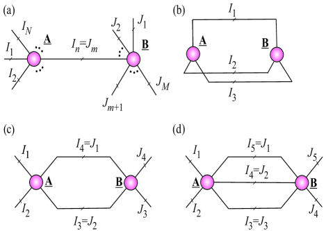
In a similar way to mode-n𝑛n multilinear product, we can define the mode-(nm)(_{n}^{m}) product of two tensors (tensor contraction) 𝐀¯I1×I2××IN¯𝐀superscriptsubscript𝐼1subscript𝐼2subscript𝐼𝑁\underline{{\bf A}}\in\mathbb{R}^{I_{1}\times I_{2}\times\ldots\times I_{N}} and 𝐁¯J1×J2××JM¯𝐁superscriptsubscript𝐽1subscript𝐽2subscript𝐽𝑀\underline{{\bf B}}\in\mathbb{R}^{J_{1}\times J_{2}\times\cdots\times J_{M}}, with common modes In=Jmsubscript𝐼𝑛subscript𝐽𝑚I_{n}=J_{m} that yields an (N+M2)𝑁𝑀2(N+M-2)-order tensor 𝐂¯I1×In1×In+1××IN×J1×Jm1×Jm+1××JM¯𝐂superscriptsubscript𝐼1subscript𝐼𝑛1subscript𝐼𝑛1subscript𝐼𝑁subscript𝐽1subscript𝐽𝑚1subscript𝐽𝑚1subscript𝐽𝑀\underline{{\bf C}}\in\mathbb{R}^{I_{1}\times\cdots I_{n-1}\times I_{n+1}\times\cdots\times I_{N}\times J_{1}\times\cdots J_{m-1}\times J_{m+1}\times\cdots\times J_{M}}:

𝐂¯=𝐀¯×nm𝐁¯,¯𝐂superscriptsubscript𝑛𝑚¯𝐀¯𝐁\displaystyle\underline{{\bf C}}=\underline{{\bf A}}\;{\times}_{n}^{m}\;\underline{{\bf B}}, (4)

with entries ci1,in1,in+1,iN,j1,jm1,jm+1,jM=i=1Inai1,in1,iin+1,iNbj1,jm1,i,jm+1,jMsubscript𝑐subscript𝑖1subscript𝑖𝑛1subscript𝑖𝑛1subscript𝑖𝑁subscript𝑗1subscript𝑗𝑚1subscript𝑗𝑚1subscript𝑗𝑀superscriptsubscript𝑖1subscript𝐼𝑛subscript𝑎subscript𝑖1subscript𝑖𝑛1𝑖subscript𝑖𝑛1subscript𝑖𝑁subscript𝑏subscript𝑗1subscript𝑗𝑚1𝑖subscript𝑗𝑚1subscript𝑗𝑀c_{i_{1},\ldots i_{n-1},\,i_{n+1},\ldots i_{N},\,j_{1},\ldots j_{m-1},\,j_{m+1},\ldots j_{M}}=\sum_{i=1}^{I_{n}}a_{i_{1},\ldots i_{n-1},\;i\;i_{n+1},\ldots i_{N}}b_{j_{1},\ldots j_{m-1},\;i,\;j_{m+1},\ldots j_{M}} (see Fig. 10 (a)). This operation can be considered as a contraction of two tensors in single common mode. Tensors can be contracted in several modes or even in all modes as illustrated in Fig. 10.

If not confusing a super- or sub-index m,n𝑚𝑛m,n can be neglected. For example, the multilinear product of the tensors 𝐀¯I1×I2××IN¯𝐀superscriptsubscript𝐼1subscript𝐼2subscript𝐼𝑁\underline{{\bf A}}\in\mathbb{R}^{I_{1}\times I_{2}\times\cdots\times I_{N}} and 𝐁¯J1×J2××JM¯𝐁superscriptsubscript𝐽1subscript𝐽2subscript𝐽𝑀\underline{{\bf B}}\in\mathbb{R}^{J_{1}\times J_{2}\times\cdots\times J_{M}}, with a common modes IN=J1subscript𝐼𝑁subscript𝐽1I_{N}=J_{1} can be written as

𝐂¯=𝐀¯×N1𝐁¯=𝐀¯×N𝐁¯=𝐀¯𝐁¯¯𝐂superscriptsubscript𝑁1¯𝐀¯𝐁subscript𝑁¯𝐀¯𝐁¯𝐀¯𝐁\displaystyle\underline{{\bf C}}=\underline{{\bf A}}\;\times_{N}^{1}\;\underline{{\bf B}}=\underline{{\bf A}}\times_{N}\underline{{\bf B}}=\underline{{\bf A}}\bullet\underline{{\bf B}}
I1×I2××IN1××J2××JM,absentsuperscriptsubscript𝐼1subscript𝐼2absentsubscript𝐼𝑁1absentsubscript𝐽2subscript𝐽𝑀\displaystyle\in\;\mathbb{R}^{I_{1}\times I_{2}\times\times I_{N-1}\times\times J_{2}\times\cdots\times J_{M}}, (5)

with entries: ci2,i3,,iN,j1,j3,,jM=i=1I1ai,i2,,iNbj1,i,j3,,jMsubscript𝑐subscript𝑖2subscript𝑖3subscript𝑖𝑁subscript𝑗1subscript𝑗3subscript𝑗𝑀superscriptsubscript𝑖1subscript𝐼1subscript𝑎𝑖subscript𝑖2subscript𝑖𝑁subscript𝑏subscript𝑗1𝑖subscript𝑗3subscript𝑗𝑀c_{i_{2},i_{3},\ldots,i_{N},j_{1},j_{3},\ldots,j_{M}}=\sum_{i=1}^{I_{1}}a_{i,i_{2},\ldots,i_{N}}\;b_{j_{1},i,j_{3},\ldots,j_{M}}. Furthermore, note that for multiplications of matrices and vectors this notation implies that 𝐀×21𝐁=𝐀𝐁subscriptsuperscript12𝐀𝐁𝐀𝐁{\bf A}\times^{1}_{2}{\bf B}={\bf A}{\bf B}, 𝐀×22𝐁=𝐀𝐁Tsubscriptsuperscript22𝐀𝐁superscript𝐀𝐁𝑇\;{\bf A}\times^{2}_{2}{\bf B}={\bf A}{\bf B}^{T}, 𝐀×1,21,2𝐁=𝐀,𝐁subscriptsuperscript1212𝐀𝐁𝐀𝐁\;{\bf A}\times^{1,2}_{1,2}{\bf B}=\langle{\bf A},{\bf B}\rangle, and 𝐀×21𝒙=𝐀×2𝒙=𝐀𝒙subscriptsuperscript12𝐀𝒙subscript2𝐀𝒙𝐀𝒙{\bf A}\times^{1}_{2}\mbox{\boldmath$x$}={\bf A}\times_{2}\mbox{\boldmath$x$}={\bf A}\mbox{\boldmath$x$}.

Remark: If we use contraction for more than two tensors the order has to be specified (defined) as follows:
𝐀¯×ab𝐁¯×cd𝐂¯=𝐀¯×ab(𝐁¯×cd𝐂¯)superscriptsubscript𝑐𝑑subscriptsuperscript𝑏𝑎¯𝐀¯𝐁¯𝐂subscriptsuperscript𝑏𝑎¯𝐀superscriptsubscript𝑐𝑑¯𝐁¯𝐂\underline{{\bf A}}\times^{b}_{a}\underline{{\bf B}}\times_{c}^{d}\underline{{\bf C}}=\underline{{\bf A}}\times^{b}_{a}(\underline{{\bf B}}\times_{c}^{d}\underline{{\bf C}}) for b<c𝑏𝑐b<c.

Refer to caption
Figure  10: Examples of tensor contractions: (a) Multilinear product of two tensors is denoted by 𝐂¯=𝐀¯×nm𝐁¯¯𝐂superscriptsubscript𝑛𝑚¯𝐀¯𝐁\underline{{\bf C}}=\underline{{\bf A}}\;\times_{n}^{m}\;\underline{{\bf B}}. (b) Inner product of two 3rd-order tensors yields a scalar c=𝐀¯,𝐁¯=𝐀¯×1,2,31,2,3𝐁¯=𝐀¯×𝐁¯=i1,i2,i3ai1,i2,i3bi1,i2,i3𝑐¯𝐀¯𝐁superscriptsubscript123123¯𝐀¯𝐁¯𝐀¯𝐁subscriptsubscript𝑖1subscript𝑖2subscript𝑖3subscript𝑎subscript𝑖1subscript𝑖2subscript𝑖3subscript𝑏subscript𝑖1subscript𝑖2subscript𝑖3c=\langle\underline{{\bf A}},\underline{{\bf B}}\rangle=\underline{{\bf A}}\;\times_{1,2,3}^{1,2,3}\;\underline{{\bf B}}=\underline{{\bf A}}\;\times\;\underline{{\bf B}}=\sum_{i_{1},i_{2},i_{3}}\;a_{i_{1},i_{2},i_{3}}\;b_{i_{1},i_{2},i_{3}}. (c) Tensor contraction of two 4th-order tensors yields 𝐂¯=𝐀¯×4,31,2𝐁¯I1×I2×J3×J4¯𝐂superscriptsubscript4312¯𝐀¯𝐁superscriptsubscript𝐼1subscript𝐼2subscript𝐽3subscript𝐽4\underline{{\bf C}}=\underline{{\bf A}}\;\times_{4,3}^{1,2}\;\underline{{\bf B}}\in\mathbb{R}^{I_{1}\times I_{2}\times J_{3}\times J_{4}}, with entries ci1,i2,j3,j4=i3,i4ai1,i2,i3,i4bi4,i3,j3,j4subscript𝑐subscript𝑖1subscript𝑖2subscript𝑗3subscript𝑗4subscriptsubscript𝑖3subscript𝑖4subscript𝑎subscript𝑖1subscript𝑖2subscript𝑖3subscript𝑖4subscript𝑏subscript𝑖4subscript𝑖3subscript𝑗3subscript𝑗4c_{i_{1},i_{2},j_{3},j_{4}}=\sum_{i_{3},i_{4}}\;a_{i_{1},i_{2},i_{3},i_{4}}\;b_{i_{4},i_{3},j_{3},j_{4}}. (d) Tensor contraction of two 5th-order tensors yields 4th-order tensor 𝐂¯=𝐀¯×3,4,51,2,3𝐁¯I1×I2×J4×J5¯𝐂superscriptsubscript345123¯𝐀¯𝐁superscriptsubscript𝐼1subscript𝐼2subscript𝐽4subscript𝐽5\underline{{\bf C}}=\underline{{\bf A}}\;\times_{3,4,5}^{1,2,3}\;\underline{{\bf B}}\in\mathbb{R}^{I_{1}\times I_{2}\times J_{4}\times J_{5}}, with entries ci1,i2,j4,j5=i3,i4,i5ai1,i2,i3,i4,i5bi5,i4,i3,j4,j5subscript𝑐subscript𝑖1subscript𝑖2subscript𝑗4subscript𝑗5subscriptsubscript𝑖3subscript𝑖4subscript𝑖5subscript𝑎subscript𝑖1subscript𝑖2subscript𝑖3subscript𝑖4subscript𝑖5subscript𝑏subscript𝑖5subscript𝑖4subscript𝑖3subscript𝑗4subscript𝑗5c_{i_{1},i_{2},j_{4},j_{5}}=\sum_{i_{3},i_{4},i_{5}}\;a_{i_{1},i_{2},i_{3},i_{4},i_{5}}\;b_{i_{5},i_{4},i_{3},j_{4},j_{5}}.

The outer or tensor product 𝐂¯=𝐀¯𝐁¯¯𝐂¯𝐀¯𝐁\underline{{\bf C}}=\underline{{\bf A}}\circ\underline{{\bf B}} of the tensors 𝐀¯I1××IN¯𝐀superscriptsubscript𝐼1subscript𝐼𝑁\underline{{\bf A}}\in\mathbb{R}^{I_{1}\times\cdots\times I_{N}} and 𝐁¯J1××JM¯𝐁superscriptsubscript𝐽1subscript𝐽𝑀\underline{{\bf B}}\in\mathbb{R}^{J_{1}\times\cdots\times J_{M}} is the tensor 𝐂¯I1××IN×J1××JM¯𝐂superscriptsubscript𝐼1subscript𝐼𝑁subscript𝐽1subscript𝐽𝑀\underline{{\bf C}}\in\mathbb{R}^{I_{1}\times\cdots\times I_{N}\times J_{1}\times\cdots\times J_{M}}, with entries ci1,,iN,j1,,jM=ai1,,iNbj1,,jMsubscript𝑐subscript𝑖1subscript𝑖𝑁subscript𝑗1subscript𝑗𝑀subscript𝑎subscript𝑖1subscript𝑖𝑁subscript𝑏subscript𝑗1subscript𝑗𝑀c_{i_{1},\ldots,i_{N},j_{1},\ldots,j_{M}}=a_{i_{1},\ldots,i_{N}}\;b_{j_{1},\ldots,j_{M}}. Specifically, the outer product of two nonzero vectors 𝒂I,𝒃Jformulae-sequence𝒂superscript𝐼𝒃superscript𝐽\mbox{\boldmath$a$}\in\mathbb{R}^{I},\;\mbox{\boldmath$b$}\in\mathbb{R}^{J} produces a rank-1 matrix 𝐗=𝒂𝒃=𝒂𝒃TI×J𝐗𝒂𝒃superscript𝒂𝒃𝑇superscript𝐼𝐽{\bf X}=\mbox{\boldmath$a$}\circ\mbox{\boldmath$b$}=\mbox{\boldmath$a$}\mbox{\boldmath$b$}^{T}\in\mathbb{R}^{I\times J} and the outer product of three nonzero vectors: 𝒂I,𝒃Jformulae-sequence𝒂superscript𝐼𝒃superscript𝐽\mbox{\boldmath$a$}\in\mathbb{R}^{I},\;\mbox{\boldmath$b$}\in\mathbb{R}^{J} and 𝒄K𝒄superscript𝐾\mbox{\boldmath$c$}\in\mathbb{R}^{K} produces a 3rd-order rank-1 tensor: 𝐗¯=𝒂𝒃𝒄I×J×K¯𝐗𝒂𝒃𝒄superscript𝐼𝐽𝐾\underline{{\bf X}}=\mbox{\boldmath$a$}\circ\mbox{\boldmath$b$}\circ\mbox{\boldmath$c$}\in\mathbb{R}^{I\times J\times K}, whose entries are xijk=aibjcksubscript𝑥𝑖𝑗𝑘subscript𝑎𝑖subscript𝑏𝑗subscript𝑐𝑘x_{ijk}=a_{i}\;b_{j}\;c_{k}. A tensor 𝐗¯I1×I2××IN¯𝐗superscriptsubscript𝐼1subscript𝐼2subscript𝐼𝑁\underline{{\bf X}}\in\mathbb{R}^{I_{1}\times I_{2}\times\cdots\times I_{N}} is said to be rank-1 if it can be expressed exactly as 𝐗¯=𝒃1𝒃2𝒃N¯𝐗subscript𝒃1subscript𝒃2subscript𝒃𝑁\underline{{\bf X}}=\mbox{\boldmath$b$}_{1}\circ\mbox{\boldmath$b$}_{2}\circ\cdots\circ\mbox{\boldmath$b$}_{N}, with entries xi1,i2,,iN=bi1bi2biNsubscript𝑥subscript𝑖1subscript𝑖2subscript𝑖𝑁subscript𝑏subscript𝑖1subscript𝑏subscript𝑖2subscript𝑏subscript𝑖𝑁x_{i_{1},i_{2},\ldots,i_{N}}=b_{i_{1}}b_{i_{2}}\cdots b_{i_{N}}, where 𝒃nInsubscript𝒃𝑛superscriptsubscript𝐼𝑛\mbox{\boldmath$b$}_{n}\in\mathbb{R}^{I_{n}} are nonzero vectors. We refer to [1, 4] for more detail regarding the basic notations and tensor operations.

III Tensor Networks

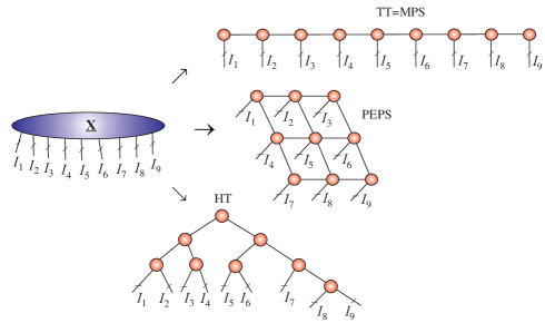
A tensor network aims to represent or decompose a higher-order tensor into a set of lower-order tensors (typically, 2nd (matrices) and 3rd-order tensors called cores or components) which are sparsely interconnected. In other words, in contrast to TDs, TNs represent decompositions of the data tensors into a set of sparsely (weakly) interconnected lower-order tensors. Recently, the curse of dimensionality for higher-order tensors has been considerably alleviated or even completely avoided through the concept of tensor networks (TN) [20, 21]. A TN can be represented by a set of nodes interconnected by lines. The lines (leads, branches, edges) connecting tensors between each other correspond to contracted modes, whereas lines that do not go from one tensor to another correspond to open (physical) modes in the TN (see Fig. 11).

An edge connecting two nodes indicates a contraction of the respective tensors in the associated pair of modes as illustrated in Fig. 10. Each free (dangling) edge corresponds to a mode, that is not contracted and, hence, the order of the entire tensor network is given by the number of free edges (called often physical indices). A tensor network may not contain any loops, i.e., any edges connecting a node with itself. Some examples of tensor network diagrams are given in Fig. 11.
Refer to caption
Figure  11: Examples of tensor networks. Illustration of representation of 9th-order tensor 𝐗¯I1×I2××I9¯𝐗superscriptsubscript𝐼1subscript𝐼2subscript𝐼9\underline{{\bf X}}\in\mathbb{R}^{I_{1}\times I_{2}\times\cdots\times I_{9}} by different kinds of tensor networks (TNs): Tensor Train (TT) which is equivalent to the Matrix Product State (MPS) (with open boundary conditions (OBC)), the Projected Entangled-Pair State (PEPS), called also Tensor Product States (TPS, and Hierarchical Tucker (HT) decomposition, which is equivalent to the Tree-Tensor Network State (TTNS). The objective is to decompose a high-order tensor into sparsely connected low-order and low-rank tensors, typically 3rd-order and/or 4th-order tensors, called cores.

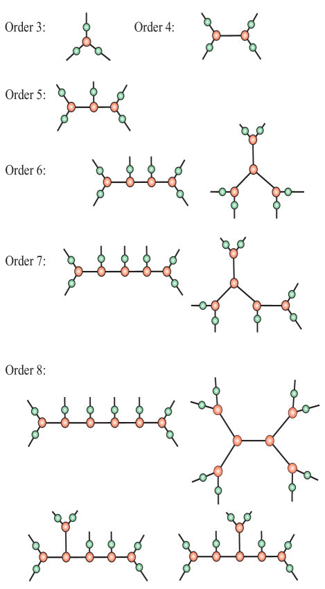
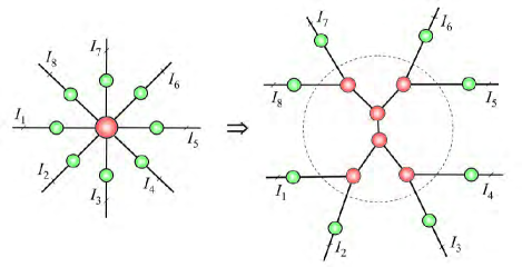
If a tensor network is a tree, i.e., it does not contain any cycle, each of its edges splits the modes of the data tensor into two groups, which is related to the suitable matricization of the tensor. If, in such a tree tensor network, all nodes have degree 3 or less, it corresponds to an Hierarchical Tucker (HT) decomposition shown in Fig. 12 (a). The HT decomposition has been first introduced in scientific computing by Hackbusch and Kühn and further developed by Grasedyck, Kressner, Tobler and others [22, 7, 23, 24, 25, 26]. Note that for 6th-order tensor, there are two such tensor networks (see Fig. 12 (b)), and for 10th-order there are 11 possible HT decompositions [24, 25].

(a)
Refer to caption
(b)
Refer to caption

Figure  12: (a) The standard Tucker decomposition and its transformation into Hierarchical Tucker (HT) model for an 8th-order tensor using interconnected 3rd-order core tensors. (b) Various exemplary structure HT/TT models for different order of data tensors. Green circles indicate factor matrices while red circles indicate cores.

A simple approach to reduce the size of core tensors is to apply distributed tensor networks (DTNs), which consists in two kinds of cores (nodes): Internal cores (nodes) which have no free edges and external cores which have free edges representing physical indices of a data tensor as illustrated in Figs. 12 and 13.

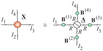
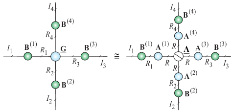
The idea in the case of the Tucker model, is that a core tensor is replaced by distributed sparsely interconnected cores of lower-order, resulting in a Hierarchical Tucker (HT) network in which only some cores are connected (associated) directly with factor matrices [7, 23, 26, 22].

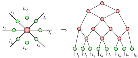
For some very high-order data tensors it has been observed that the ranks Rnsubscript𝑅𝑛R_{n} (internal dimensions of cores) increase rapidly with the order of the tensor and/or with an increasing accuracy of approximation for any choice of tensor network, that is, a tree (including TT and HT decompositions) [25]. For such cases, the Projected Entangled-Pair State (PEPS) or the Multi-scale Entanglement Renormalization Ansatz (MERA) tensor networks can be used. These contain cycles, but have hierarchical structures (see Fig. 13). For the PEPS and MERA TNs the ranks can be kept considerably smaller, at the cost of employing 5th and 4th-order cores and consequently a higher computational complexity w.r.t. tensor contractions. The main advantage of PEPS and MERA is that the size of each core tensor in the internal tensor network structure is usually much smaller than the cores in TT/HT decompositions, so consequently the total number of parameters can be reduced. However, it should be noted that the contraction of the resulting tensor network becomes more difficult when compared to the basic tree structures represented by TT and HT models. This is due to the fact that the PEPS and MERA tensor networks contain loops.
Refer to caption
Figure  13: Alternative distributed representation of 8th-order Tucker decomposition where a core tensor is replaced by MERA (Multi-scale Entanglement Renormalization Ansatz) tensor network which employs 3rd-order and 4th-order core tensors. For some data-sets, the advantage of such model is relatively low size (dimensions) of the distributed cores.

IV Basic Tensor Decompositions and their Representation via Tensor Networks Diagrams

The main objective of a standard tensor decomposition is to factorize a data tensor into physically interpretable or meaningful factor matrices and a single core tensor which indicates the links between components (vectors of factor matrices) in different modes.

IV-A Constrained Matrix Factorizations and Decompositions – Two-Way Component Analysis

Two-way Component Analysis (2-way CA) exploits a priori knowledge about different characteristics, features or morphology of components (or source signals) [1, 27] to find the hidden components thorough constrained matrix factorizations of the form

𝐗=𝐀𝐁T+𝐄=r=1R𝒂r𝒃r+𝐄=r=1R𝒂r𝒃rT+𝐄,𝐗superscript𝐀𝐁𝑇𝐄superscriptsubscript𝑟1𝑅subscript𝒂𝑟subscript𝒃𝑟𝐄superscriptsubscript𝑟1𝑅subscript𝒂𝑟subscriptsuperscript𝒃𝑇𝑟𝐄{\bf X}={\bf A}{\bf B}^{T}+{\bf E}=\sum_{r=1}^{R}\mbox{\boldmath$a$}_{r}\circ\mbox{\boldmath$b$}_{r}+{\bf E}=\sum_{r=1}^{R}\mbox{\boldmath$a$}_{r}\mbox{\boldmath$b$}^{T}_{r}+{\bf E}, (6)

where the constraints imposed on factor matrices 𝐀𝐀{\bf A} and/or 𝐁𝐁{\bf B} include orthogonality, sparsity, statistical independence, nonnegativity or smoothness. The CA can be considered as a bilinear (2-way) factorization, where 𝐗I×J𝐗superscript𝐼𝐽{\bf X}\in\mathbb{R}^{I\times J} is a known matrix of observed data, 𝐄I×J𝐄superscript𝐼𝐽{\bf E}\in\mathbb{R}^{I\times J} represents residuals or noise, 𝐀=[𝒂1,𝒂2,,𝒂R]I×R𝐀subscript𝒂1subscript𝒂2subscript𝒂𝑅superscript𝐼𝑅{\bf A}=[\mbox{\boldmath$a$}_{1},\mbox{\boldmath$a$}_{2},\ldots,\mbox{\boldmath$a$}_{R}]\in\mathbb{R}^{I\times R} is the unknown (usually, full column rank R𝑅R) mixing matrix with R𝑅R basis vectors 𝒂rIsubscript𝒂𝑟superscript𝐼\mbox{\boldmath$a$}_{r}\in\mathbb{R}^{I}, and 𝐁=[𝒃1,𝒃2,{\bf B}=[\mbox{\boldmath$b$}_{1},\mbox{\boldmath$b$}_{2}, ,𝒃R]\ldots,\mbox{\boldmath$b$}_{R}] J×Rabsentsuperscript𝐽𝑅\in\mathbb{R}^{J\times R} is the matrix of unknown components (factors, latent variables, sources).

Two-way component analysis (CA) refers to a class of signal processing techniques that decompose or encode superimposed or mixed signals into components with certain constraints or properties. The CA methods exploit a priori knowledge about the true nature or diversities of latent variables. By diversity, we refer to different characteristics, features or morphology of sources or hidden latent variables [27].

For example, the columns of the matrix 𝐁𝐁{\bf B} that represent different data sources should be: as statistically independent as possible for ICA; as sparse as possible for SCA; take only nonnegative values for (NMF) [1, 27, 16].

Remark: Note that matrix factorizations have an inherent symmetry, Eq. (6) could be written as 𝐗T𝐁𝐀Tsuperscript𝐗𝑇superscript𝐁𝐀𝑇{\bf X}^{T}\approx{\bf B}{\bf A}^{T}, thus interchanging the roles of sources and mixing process.

Singular value decomposition (SVD) of the data matrix 𝐗I×J𝐗superscript𝐼𝐽{\bf X}\in\mathbb{R}^{I\times J} is a special case of the factorization in Eq. (6). It is exact and provides an explicit notion of the range and null space of the matrix 𝐗𝐗{\bf X} (key issues in low-rank approximation), and is given by

𝐗=𝐔𝚺𝐕T=r=1Rσr𝒖r𝒗rT=r=1Rσr𝒖r𝒗r,𝐗𝐔𝚺superscript𝐕𝑇superscriptsubscript𝑟1𝑅subscript𝜎𝑟subscript𝒖𝑟superscriptsubscript𝒗𝑟𝑇superscriptsubscript𝑟1𝑅subscript𝜎𝑟subscript𝒖𝑟subscript𝒗𝑟{\bf X}={\bf U}\mbox{\boldmath$\Sigma$}{\bf V}^{T}=\sum_{r=1}^{R}\sigma_{r}\;\mbox{\boldmath$u$}_{r}\mbox{\boldmath$v$}_{r}^{T}=\sum_{r=1}^{R}\sigma_{r}\;\mbox{\boldmath$u$}_{r}\circ\mbox{\boldmath$v$}_{r}, (7)

where 𝐔𝐔{\bf U} and 𝐕𝐕{\bf V} are column-wise orthonormal matrices and 𝚺𝚺\Sigma is a diagonal matrix containing only nonnegative singular values σrsubscript𝜎𝑟\sigma_{r}.

Another virtue of component analysis comes from a representation of multiple-subject, multiple-task datasets by a set of data matrices 𝐗ksubscript𝐗𝑘{\bf X}_{k}, allowing us to perform simultaneous matrix factorizations:

𝐗k𝐀k𝐁kT,(k=1,2,,K),subscript𝐗𝑘subscript𝐀𝑘superscriptsubscript𝐁𝑘𝑇𝑘12𝐾\displaystyle{\bf X}_{k}\approx{\bf A}_{k}{\bf B}_{k}^{T},\qquad(k=1,2,\ldots,K), (8)

subject to various constraints. In the case of statistical independence constraints, the problem can be related to models of group ICA through suitable pre-processing, dimensionality reduction and post-processing procedures [28].

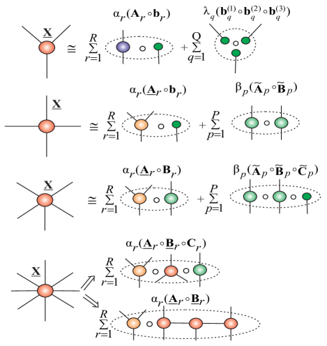
The field of CA is maturing and has generated efficient algorithms for 2-way component analysis (especially, for sparse/functional PCA/SVD, ICA, NMF and SCA) [16, 1, 29]. The rapidly emerging field of tensor decompositions is the next important step that naturally generalizes 2-way CA/BSS algorithms and paradigms. We proceed to show how constrained matrix factorizations and component analysis (CA) models can be naturally generalized to multilinear models using constrained tensor decompositions, such as the Canonical Polyadic Decomposition (CPD) and Tucker models, as illustrated in Figs. 14 and 15.

IV-B The Canonical Polyadic Decomposition (CPD)

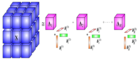
The CPD (called also PARAFAC or CANDECOMP) factorizes an N𝑁Nth-order tensor 𝐗¯I1×I2××IN¯𝐗superscriptsubscript𝐼1subscript𝐼2subscript𝐼𝑁\underline{{\bf X}}\in\mathbb{R}^{I_{1}\times I_{2}\times\cdots\times I_{N}} into a linear combination of terms 𝒃r(1)𝒃r(2)𝒃r(N)subscriptsuperscript𝒃1𝑟subscriptsuperscript𝒃2𝑟subscriptsuperscript𝒃𝑁𝑟\mbox{\boldmath$b$}^{(1)}_{r}\circ\mbox{\boldmath$b$}^{(2)}_{r}\circ\cdots\circ\mbox{\boldmath$b$}^{(N)}_{r}, which are rank-1 tensors, and is given by [30, 31, 32]

𝐗¯¯𝐗\displaystyle\underline{{\bf X}} r=1Rλr𝒃r(1)𝒃r(2)𝒃r(N)absentsuperscriptsubscript𝑟1𝑅subscript𝜆𝑟subscriptsuperscript𝒃1𝑟subscriptsuperscript𝒃2𝑟subscriptsuperscript𝒃𝑁𝑟\displaystyle\cong\sum_{r=1}^{R}\lambda_{r}\;\mbox{\boldmath$b$}^{(1)}_{r}\circ\mbox{\boldmath$b$}^{(2)}_{r}\circ\cdots\circ\mbox{\boldmath$b$}^{(N)}_{r} (9)
=𝚲¯×1𝐁(1)×2𝐁(2)×N𝐁(N)absentsubscript𝑁subscript2subscript1¯𝚲superscript𝐁1superscript𝐁2superscript𝐁𝑁\displaystyle=\underline{\mbox{\boldmath$\Lambda$}}\times_{1}{\bf B}^{(1)}\times_{2}{\bf B}^{(2)}\cdots\times_{N}{\bf B}^{(N)}
=𝚲¯;𝐁(1),𝐁(2),,𝐁(N),absent¯𝚲superscript𝐁1superscript𝐁2superscript𝐁𝑁\displaystyle=\llbracket\underline{\mbox{\boldmath$\Lambda$}};\mathbf{B}^{(1)},\mathbf{B}^{(2)},\ldots,\mathbf{B}^{(N)}\rrbracket,

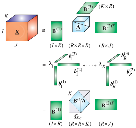
where the only non-zero entries λrsubscript𝜆𝑟\lambda_{r} of the diagonal core tensor 𝐆¯=𝚲¯R×R××R¯𝐆¯𝚲superscript𝑅𝑅𝑅\underline{{\bf G}}=\underline{\mbox{\boldmath$\Lambda$}}\in\mathbb{R}^{R\times R\times\cdots\times R} are located on the main diagonal (see Fig. 14 for a 3rd-order and 4th-order tensors).

Via the Khatri-Rao products the CPD can also be expressed in a matrix/vector form as:

𝐗(n)𝐁(n)𝚲(𝐁(1)𝐁(n1)𝐁(n+1)𝐁(N))Tsubscript𝐗𝑛superscript𝐁𝑛𝚲superscriptdirect-productsuperscript𝐁1superscript𝐁𝑛1superscript𝐁𝑛1superscript𝐁𝑁𝑇{\bf X}_{(n)}\cong{\bf B}^{(n)}\mbox{\boldmath$\Lambda$}({\bf B}^{(1)}\odot\cdots\odot{\bf B}^{(n-1)}\odot{\bf B}^{(n+1)}\odot\cdots\odot{\bf B}^{(N)})^{T}\\
vec(𝐗¯)[𝐁(1)𝐁(2)𝐁(N)]𝝀,vec¯𝐗delimited-[]direct-productsuperscript𝐁1superscript𝐁2superscript𝐁𝑁𝝀\displaystyle\text{vec}(\underline{{\bf X}})\cong[{\bf B}^{(1)}\odot{\bf B}^{(2)}\odot\cdots\odot{\bf B}^{(N)}]\;\mbox{\boldmath$\lambda$}, (10)

where 𝐁(n)=[𝒃1(n),𝒃2(n),,𝒃R(n)]In×Rsuperscript𝐁𝑛superscriptsubscript𝒃1𝑛superscriptsubscript𝒃2𝑛superscriptsubscript𝒃𝑅𝑛superscriptsubscript𝐼𝑛𝑅{\bf B}^{(n)}=[\mbox{\boldmath$b$}_{1}^{(n)},\mbox{\boldmath$b$}_{2}^{(n)},\ldots,\mbox{\boldmath$b$}_{R}^{(n)}]\in\mathbb{R}^{I_{n}\times R}, 𝝀=[λ1,λ2,,λR]T𝝀superscriptsubscript𝜆1subscript𝜆2subscript𝜆𝑅𝑇\mbox{\boldmath$\lambda$}=[\lambda_{1},\lambda_{2},\ldots,\lambda_{R}]^{T} and 𝚲=diag{𝝀}𝚲diag𝝀\mbox{\boldmath$\Lambda$}=\mathop{\rm diag}\nolimits\{\mbox{\boldmath$\lambda$}\} is a diagonal matrix.

(a) Standard block diagram
Refer to caption

(b) CPD in tensor network notation

Refer to caption
Figure  14: Representation of the CPD. (a) The Canonical Polyadic Decomposition (CPD) of a 3rd-order tensor as: 𝐗¯𝚲¯×1𝐁(1)×2𝐁(2)×3𝐁(3)=r=1Rλr𝒃r(1)𝒃r(2)𝒃r(3)=𝐆¯c×1𝐁(1)×2𝐁(2)¯𝐗subscript3subscript2subscript1¯𝚲superscript𝐁1superscript𝐁2superscript𝐁3superscriptsubscript𝑟1𝑅subscript𝜆𝑟subscriptsuperscript𝒃1𝑟subscriptsuperscript𝒃2𝑟subscriptsuperscript𝒃3𝑟subscript2subscript1subscript¯𝐆𝑐superscript𝐁1superscript𝐁2\underline{{\bf X}}\cong\underline{\mbox{\boldmath$\Lambda$}}\times_{1}{\bf B}^{(1)}\times_{2}{\bf B}^{(2)}\times_{3}{\bf B}^{(3)}=\sum_{r=1}^{R}\lambda_{r}\;\mbox{\boldmath$b$}^{(1)}_{r}\circ\mbox{\boldmath$b$}^{(2)}_{r}\circ\mbox{\boldmath$b$}^{(3)}_{r}=\underline{{\bf G}}_{c}\times_{1}{\bf B}^{(1)}\times_{2}{\bf B}^{(2)} with 𝐆¯=𝚲¯¯𝐆¯𝚲\underline{{\bf G}}=\underline{\mbox{\boldmath$\Lambda$}} and 𝐆¯c=𝚲¯×3𝐁(3)subscript¯𝐆𝑐subscript3¯𝚲superscript𝐁3\underline{{\bf G}}_{c}=\underline{\mbox{\boldmath$\Lambda$}}\times_{3}{\bf B}^{(3)}. (b) The CPD for a 4th-order tensor as: 𝐗¯𝚲¯×1𝐁(1)×2𝐁(2)×3𝐁(3)×4𝐁(4)=r=1R𝒃r(1)𝒃r(2)𝒃r(3)𝒃r(4)¯𝐗subscript4subscript3subscript2subscript1¯𝚲superscript𝐁1superscript𝐁2superscript𝐁3superscript𝐁4superscriptsubscript𝑟1𝑅subscriptsuperscript𝒃1𝑟subscriptsuperscript𝒃2𝑟subscriptsuperscript𝒃3𝑟subscriptsuperscript𝒃4𝑟\underline{{\bf X}}\cong\underline{\mbox{\boldmath$\Lambda$}}\times_{1}{\bf B}^{(1)}\times_{2}{\bf B}^{(2)}\times_{3}{\bf B}^{(3)}\times_{4}{\bf B}^{(4)}=\sum_{r=1}^{R}\mbox{\boldmath$b$}^{(1)}_{r}\circ\mbox{\boldmath$b$}^{(2)}_{r}\circ\mbox{\boldmath$b$}^{(3)}_{r}\circ\mbox{\boldmath$b$}^{(4)}_{r}. The objective of the CPD is to estimate the factor matrices 𝐁(n)superscript𝐁𝑛{\bf B}^{(n)} and a rank of tensor R𝑅R, that is, the number of components R𝑅R.

The rank of tensor 𝐗¯¯𝐗\underline{{\bf X}} is defined as the smallest R𝑅R for which CPD (9) holds exactly.

Algorithms to compute CPD. In the presence of noise in real world applications the CPD is rarely exact and has to be estimated by minimizing a suitable cost function, typically of the Least-Squares (LS) type in the form of the Frobenius norm 𝐗¯𝚲¯;𝐁(1),𝐁(2),,𝐁(N)Fsubscriptnorm¯𝐗¯𝚲superscript𝐁1superscript𝐁2superscript𝐁𝑁𝐹||\underline{{\bf X}}-\llbracket\underline{\mbox{\boldmath$\Lambda$}};\mathbf{B}^{(1)},\mathbf{B}^{(2)},\ldots,\mathbf{B}^{(N)}\rrbracket||_{F}, or using Least Absolute Error (LAE) criteria [33]. The Alternating Least Squares (ALS) algorithms [13, 31, 1, 34] minimize the LS cost function by optimizing individually each component matrix, while keeping the other component matrices fixed. For instance, assume that the diagonal matrix 𝚲𝚲\Lambda has been absorbed in one of the component matrices; then, by taking advantage of the Khatri-Rao structure the component matrices 𝐁(n)superscript𝐁𝑛{\bf B}^{(n)} can be updated sequentially as [4]

𝐁(n)𝐗(n)(kn𝐁(k))(kn(𝐁(k)T𝐁(k))),\displaystyle{\bf B}^{(n)}\leftarrow{\bf X}_{(n)}\left(\bigodot_{k\neq n}{\bf B}^{(k)}\right)\left(\circledast_{k\neq n}({\bf B}^{(k)\;T}{\bf B}^{(k)})\right)^{\dagger}, (11)

which requires the computation of the pseudo-inverse of small (R×R)𝑅𝑅(R\times R) matrices.

The ALS is attractive for its simplicity and for well defined problems (not too many, well separated, not collinear components) and high SNR, the performance of ALS algorithms is often satisfactory. For ill-conditioned problems, more advanced algorithms exist, which typically exploit the rank-1 structure of the terms within CPD to perform efficient computation and storage of the Jacobian and Hessian of the cost function [35, 36].

Constraints. The CPD is usually unique by itself, and does not require constraints to impose uniqueness [37]. However, if components in one or more modes are known to be e.g., nonnegative, orthogonal, statistically independent or sparse, these constraints should be incorporated to relax uniqueness conditions. More importantly, constraints may increase the accuracy and stability of the CPD algorithms and facilitate better physical interpretability of components [38, 39].

IV-C The Tucker Decomposition

The Tucker decomposition can be expressed as follows [40]:

𝐗¯¯𝐗\displaystyle\underline{{\bf X}} \displaystyle\cong r1=1R1rN=1RNgr1r2rN(𝒃r1(1)𝒃r2(2)𝒃rN(N))superscriptsubscriptsubscript𝑟11subscript𝑅1superscriptsubscriptsubscript𝑟𝑁1subscript𝑅𝑁subscript𝑔subscript𝑟1subscript𝑟2subscript𝑟𝑁subscriptsuperscript𝒃1subscript𝑟1subscriptsuperscript𝒃2subscript𝑟2subscriptsuperscript𝒃𝑁subscript𝑟𝑁\displaystyle\sum\limits_{r_{1}=1}^{R_{1}}{{\cdots\sum\limits_{r_{N}=1}^{R_{N}}{g_{r_{1}r_{2}\cdots r_{N}}\,\left(\;\mbox{\boldmath$b$}^{(1)}_{r_{1}}\circ\mbox{\boldmath$b$}^{(2)}_{r_{2}}\circ\cdots\circ\mbox{\boldmath$b$}^{(N)}_{r_{N}}\right)}}} (12)
=\displaystyle= 𝐆¯×1𝐁(1)×2𝐁(2)×N𝐁(N)subscript𝑁subscript2subscript1¯𝐆superscript𝐁1superscript𝐁2superscript𝐁𝑁\displaystyle\underline{{\bf G}}\times_{1}{\bf B}^{(1)}\times_{2}{\bf B}^{(2)}\cdots\times_{N}{\bf B}^{(N)}
=\displaystyle= 𝐆¯;𝐁(1),𝐁(2),,𝐁(N).¯𝐆superscript𝐁1superscript𝐁2superscript𝐁𝑁\displaystyle\llbracket\underline{{\bf G}};{\bf B}^{(1)},{\bf B}^{(2)},\ldots,{\bf B}^{(N)}\rrbracket.

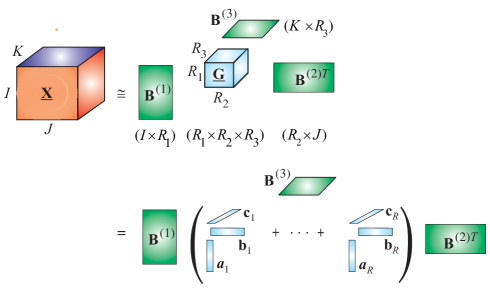
where 𝐗¯I1×I2××IN¯𝐗superscriptsubscript𝐼1subscript𝐼2subscript𝐼𝑁\underline{{\bf X}}\in\mathbb{R}^{I_{1}\times I_{2}\times\cdots\times I_{N}} is the given data tensor, 𝐆¯R1×R2××RN¯𝐆superscriptsubscript𝑅1subscript𝑅2subscript𝑅𝑁\underline{{\bf G}}\in\mathbb{R}^{R_{1}\times R_{2}\times\cdots\times R_{N}} is the core tensor and 𝐁(n)=[𝒃1(n),𝒃2(n),,𝒃Rn(n)]In×Rnsuperscript𝐁𝑛superscriptsubscript𝒃1𝑛superscriptsubscript𝒃2𝑛superscriptsubscript𝒃subscript𝑅𝑛𝑛superscriptsubscript𝐼𝑛subscript𝑅𝑛{\bf B}^{(n)}=[\mbox{\boldmath$b$}_{1}^{(n)},\mbox{\boldmath$b$}_{2}^{(n)},\ldots,\mbox{\boldmath$b$}_{R_{n}}^{(n)}]\in\mathbb{R}^{I_{n}\times R_{n}} are the mode-n𝑛n component matrices, n=1,2,,N𝑛12𝑁n=1,2,\ldots,N (see Fig. 15).

(a) Standard block diagram of TD
Refer to caption

(b) TD in tensor network notations

Refer to caption
Figure  15: Representation of the Tucker Decomposition (TD). (a) TD of a 3rd-order tensor 𝐗¯𝐆¯×1𝐁(1)×2𝐁(2)×3𝐁(3)¯𝐗subscript3subscript2subscript1¯𝐆superscript𝐁1superscript𝐁2superscript𝐁3\underline{{\bf X}}\cong\underline{{\bf G}}\times_{1}{\bf B}^{(1)}\times_{2}{\bf B}^{(2)}\times_{3}{\bf B}^{(3)}. The objective is to compute factor matrices 𝐁(n)superscript𝐁𝑛{\bf B}^{(n)} and core tensor 𝐆¯¯𝐆\underline{{\bf G}}. In some applications, in the second stage, the core tensor is approximately factorized using the CPD as 𝐆¯r=1R𝒂r𝒃r𝒄r¯𝐆superscriptsubscript𝑟1𝑅subscript𝒂𝑟subscript𝒃𝑟subscript𝒄𝑟\underline{{\bf G}}\cong\sum_{r=1}^{R}\mbox{\boldmath$a$}_{r}\circ\mbox{\boldmath$b$}_{r}\circ\mbox{\boldmath$c$}_{r}. (b) Graphical representation of the Tucker and CP decompositions in two-stage procedure for a 4th-order tensor as: 𝐗¯𝐆¯×1𝐁(1)×2𝐁(2)×4𝐁(4)=𝐆¯;𝐁(1),𝐁(2),𝐁(3),𝐁(4)(𝚲¯×1𝐀(1)×2𝐀(2)×4𝐀(4))×1𝐁(1)×2𝐁(2)×4𝐁(4)=𝚲¯;𝐁(1)𝐀(1),𝐁(2)𝐀(2),𝐁(3)𝐀(3),𝐁(4)𝐀(4)¯𝐗subscript4subscript2subscript1¯𝐆superscript𝐁1superscript𝐁2superscript𝐁4¯𝐆superscript𝐁1superscript𝐁2superscript𝐁3superscript𝐁4subscript4subscript2subscript1subscript4subscript2subscript1¯𝚲superscript𝐀1superscript𝐀2superscript𝐀4superscript𝐁1superscript𝐁2superscript𝐁4¯𝚲superscript𝐁1superscript𝐀1superscript𝐁2superscript𝐀2superscript𝐁3superscript𝐀3superscript𝐁4superscript𝐀4\underline{{\bf X}}\cong\underline{{\bf G}}\times_{1}{\bf B}^{(1)}\times_{2}{\bf B}^{(2)}\cdots\times_{4}{\bf B}^{(4)}=\llbracket\underline{{\bf G}};{\bf B}^{(1)},{\bf B}^{(2)},{\bf B}^{(3)},{\bf B}^{(4)}\rrbracket\cong(\underline{\mbox{\boldmath$\Lambda$}}\times_{1}{\bf A}^{(1)}\times_{2}{\bf A}^{(2)}\cdots\times_{4}{\bf A}^{(4)})\times_{1}{\bf B}^{(1)}\times_{2}{\bf B}^{(2)}\cdots\times_{4}{\bf B}^{(4)}=\llbracket\underline{\mbox{\boldmath$\Lambda$}};\;{\bf B}^{(1)}{\bf A}^{(1)},\;{\bf B}^{(2)}{\bf A}^{(2)},\;{\bf B}^{(3)}{\bf A}^{(3)},\;{\bf B}^{(4)}{\bf A}^{(4)}\rrbracket.

Using Kronecker products the decomposition in (12) can be expressed in a matrix and vector form as follows:

𝐗(n)𝐁(n)𝐆(n)(𝐁(1)𝐁(n1)𝐁(n+1)𝐁(N))Tsubscript𝐗𝑛superscript𝐁𝑛subscript𝐆𝑛superscripttensor-producttensor-productsuperscript𝐁1superscript𝐁𝑛1superscript𝐁𝑛1superscript𝐁𝑁𝑇{\bf X}_{(n)}\cong{\bf B}^{(n)}{\bf G}_{(n)}({\bf B}^{(1)}\cdots\otimes{\bf B}^{(n-1)}\otimes{\bf B}^{(n+1)}\cdots\otimes{\bf B}^{(N)})^{T}
vec(𝐗¯)[𝐁(1)𝐁(2)𝐁(N)]vec(𝐆¯).vec¯𝐗delimited-[]tensor-producttensor-productsuperscript𝐁1superscript𝐁2superscript𝐁𝑁vec¯𝐆\displaystyle\text{vec}(\underline{{\bf X}})\cong[{\bf B}^{(1)}\otimes{\bf B}^{(2)}\cdots\otimes{\bf B}^{(N)}]\text{vec}(\underline{{\bf G}}). (13)

(a)

Refer to caption

(b)

Refer to caption
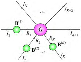
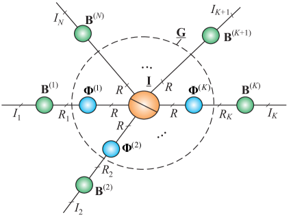
Figure  16: Graphical illustration of constrained Tucker and CPD models: (a) Tucker-(K,N)𝐾𝑁(K,N) decomposition of a N𝑁Nth-order tensor, with NK𝑁𝐾N\geq K, 𝐗¯𝐆¯×1𝐁(1)×2𝐁(2)×K𝐁(K)×K+1𝐈×K+2×N𝐈=𝐆¯;𝐁(1),𝐁(2),,𝐁(K)¯𝐗subscript𝑁subscript𝐾2subscript𝐾1subscript𝐾subscript2subscript1¯𝐆superscript𝐁1superscript𝐁2superscript𝐁𝐾𝐈𝐈¯𝐆superscript𝐁1superscript𝐁2superscript𝐁𝐾\underline{{\bf X}}\cong\underline{{\bf G}}\times_{1}{\bf B}^{(1)}\times_{2}{\bf B}^{(2)}\cdots\times_{K}{\bf B}^{(K)}\times_{K+1}{\bf I}\times_{K+2}\cdots\times_{N}{\bf I}=\llbracket\underline{{\bf G}};{\bf B}^{(1)},{\bf B}^{(2)},\ldots,{\bf B}^{(K)}\rrbracket, (b) Constrained CPD model, called PARALIND/CONFAC-(K,N)𝐾𝑁(K,N) 𝐗¯𝐆¯×1𝐁(1)×2𝐁(2)×N𝐁(N)=𝐈¯;𝐁(1)Φ(1),𝐁(2)Φ(2),,𝐁(K)Φ(K),𝐁(K+1),,𝐁(N)¯𝐗subscript𝑁subscript2subscript1¯𝐆superscript𝐁1superscript𝐁2superscript𝐁𝑁¯𝐈superscript𝐁1superscriptΦ1superscript𝐁2superscriptΦ2superscript𝐁𝐾superscriptΦ𝐾superscript𝐁𝐾1superscript𝐁𝑁\underline{{\bf X}}\cong\underline{{\bf G}}\times_{1}{\bf B}^{(1)}\times_{2}{\bf B}^{(2)}\cdots\times_{N}{\bf B}^{(N)}=\llbracket\underline{{\bf I}};{\bf B}^{(1)}\Phi^{(1)},{\bf B}^{(2)}\Phi^{(2)},\ldots,{\bf B}^{(K)}\Phi^{(K)},{\bf B}^{(K+1)},\ldots,{\bf B}^{(N)}\rrbracket, where core tensor 𝐆=𝐈¯×1Φ(1)×2Φ(2)×KΦ(K)𝐆subscript𝐾subscript2subscript1¯𝐈superscriptΦ1superscriptΦ2superscriptΦ𝐾{\bf G}=\underline{{\bf I}}\times_{1}\Phi^{(1)}\times_{2}\Phi^{(2)}\cdots\times_{K}\Phi^{(K)} with KN𝐾𝑁K\leq N.

The core tensor (typically, Rn<Insubscript𝑅𝑛subscript𝐼𝑛R_{n}<I_{n}) models a potentially complex pattern of mutual interaction between the vectors (components) in different modes.

Multilinear rank. The N𝑁N-tuple (R1,R2,,RN)subscript𝑅1subscript𝑅2subscript𝑅𝑁(R_{1},R_{2},\ldots,R_{N}) is called the multilinear-rank of 𝐗¯¯𝐗\underline{{\bf X}}, if the Tucker decomposition holds exactly.

Note that the CPD can be considered as a special case of the Tucker decomposition, in which the core tensor has nonzero elements only on main diagonal. In contrast to the CPD the Tucker decomposition, in general, is non unique. However, constraints imposed on all factor matrices and/or core tensor can reduce the indeterminacies to only column-wise permutation and scaling [41].

In Tucker model some selected factor matrices can be identity matrices, this leads to Tucker-(K,N)𝐾𝑁(K,N) model, which is graphically illustrated in Fig. 16 (a). In a such model (NK)𝑁𝐾(N-K) factor matrices are equal to identity matrices. In the simplest scenario for 3rd-order tensor 𝐗¯I1×I2×I3¯𝐗superscriptsubscript𝐼1subscript𝐼2subscript𝐼3\underline{{\bf X}}\in\mathbb{R}^{I_{1}\times I_{2}\times I_{3}} the Tucker-(2,3) model, called simply Tucker-2, can be described as

𝐗¯𝐆¯×1𝐁(1)×2𝐁(2).¯𝐗subscript2subscript1¯𝐆superscript𝐁1superscript𝐁2\displaystyle\underline{{\bf X}}\cong\underline{{\bf G}}\times_{1}{\bf B}^{(1)}\times_{2}{\bf B}^{(2)}. (14)

Similarly, we can define PARALIND/CONFAC-(K,N)𝐾𝑁(K,N) models222PARALIND is abbreviation of PARAllel with LINear Dependencies, while CONFAC means CONstrained FACtor model (for more detail see [42] and references therein.)described as [42]

𝐗¯¯𝐗\displaystyle\underline{{\bf X}} \displaystyle\cong 𝐆¯×1𝐁(1)×2𝐁(2)×N𝐁(N)subscript𝑁subscript2subscript1¯𝐆superscript𝐁1superscript𝐁2superscript𝐁𝑁\displaystyle\underline{{\bf G}}\times_{1}{\bf B}^{(1)}\times_{2}{\bf B}^{(2)}\cdots\times_{N}{\bf B}^{(N)}
=\displaystyle= 𝐈¯;𝐁(1)Φ(1),,𝐁(K)Φ(K),𝐁(K+1),𝐁(N),¯𝐈superscript𝐁1superscriptΦ1superscript𝐁𝐾superscriptΦ𝐾superscript𝐁𝐾1superscript𝐁𝑁\displaystyle\llbracket\underline{{\bf I}};{\bf B}^{(1)}\Phi^{(1)},\ldots,{\bf B}^{(K)}\Phi^{(K)},{\bf B}^{(K+1)}\ldots,{\bf B}^{(N)}\rrbracket,

where the core tensor, called constrained tensor or interaction tensor, is expressed as

𝐆=𝐈¯×1Φ(1)×2Φ(2)×KΦ(K),𝐆subscript𝐾subscript2subscript1¯𝐈superscriptΦ1superscriptΦ2superscriptΦ𝐾\displaystyle{\bf G}=\underline{{\bf I}}\times_{1}\Phi^{(1)}\times_{2}\Phi^{(2)}\cdots\times_{K}\Phi^{(K)}, (16)

with KN𝐾𝑁K\leq N. The factor matrices Φ(n)Rn×RsuperscriptΦ𝑛superscriptsubscript𝑅𝑛𝑅\Phi^{(n)}\in\mathbb{R}^{R_{n}\times R}, with Rmax(Rn)𝑅subscript𝑅𝑛R\geq\max(R_{n}) are constrained matrices, called often interaction matrices (see Fig. 16 (b).

Another important, more complex constrained CPD model, which can be represented graphically as nested Tucker-(K,N)𝐾𝑁(K,N) model is the PARATUCK-(K,N)𝐾𝑁(K,N) model (see review paper of Favier and de Almeida [42] and references therein).

IV-D Multiway Component Analysis Using Constrained Tucker Decompositions

A great success of 2-way component analysis (PCA, ICA, NMF, SCA) is largely due to the various constraints we can impose. Without constraints matrix factorization loses its most sense as the components are rather arbitrary and they do not have any physical meaning. There are various constraints that lead to all kinds of component analysis methods which are able give unique components with some desired physical meaning and properties and hence serve for different application purposes. Just similar to matrix factorization, unconstrained Tucker decompositions generally can only be served as multiway data compression as their results lack physical meaning. In the most practical applications we need to consider constrained Tucker decompositions which can provide multiple sets of essential unique components with desired physical interpretation and meaning. This is direct extension of 2-way component analysis and is referred to as multiway component analysis (MWCA) [2].

The MWCA based on Tucker-N𝑁N model can be considered as a natural and simple extension of multilinear SVD and/or multilinear ICA, in which we apply any efficient CA/BSS algorithms to each mode, which provides essential uniqueness [41].

There are two different models to interpret and implement constrained Tucker decompositions for MWCA. (1) the columns of the component matrices 𝐁(n)superscript𝐁𝑛{\bf B}^{(n)} represent the desired latent variables, the core tensor 𝐆¯¯𝐆\underline{{\bf G}} has a role of “mixing process”, modeling the links among the components from different modes, while the data tensor 𝐗¯¯𝐗\underline{{\bf X}} represents a collection of 1-D or 2-D mixing signals; (2) the core tensor represents the desired (but hidden) N𝑁N-dimensional signal (e.g., 3D MRI image or 4D video), while the component matrices represent mixing or filtering processes through e.g., time-frequency transformations or wavelet dictionaries [3].

The MWCA based on the Tucker-N𝑁N model can be computed directly in two steps: (1) for n=1,2,,N𝑛12𝑁n=1,2,\ldots,N perform model reduction and unfolding of data tensors sequentially and apply a suitable set of CA/BSS algorithms to reduced unfolding matrices 𝐗~(n)subscript~𝐗𝑛\tilde{\bf X}_{(n)}, - in each mode we can apply different constraints and algorithms; (2) compute the core tensor using e.g., the inversion formula: 𝐆¯^=𝐗¯×1𝐁(1)×2𝐁(2)×N𝐁(N)\hat{\underline{{\bf G}}}=\underline{{\bf X}}\times_{1}\mathbf{B}^{(1)}{}^{\dagger}\times_{2}\mathbf{B}^{(2)}{}^{\dagger}\cdots\times_{N}\mathbf{B}^{(N)}{}^{\dagger} [41]. This step is quite important because core tensors illuminate complex links among the multiple components in different modes [1].

(a)
Refer to caption

(b)
Refer to caption 

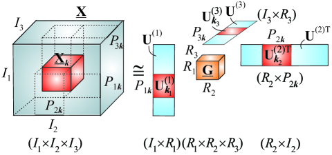
Figure  17: Conceptual models for performing the Tucker decomposition (HOSVD) for large-scale 3rd-order data tensors by dividing the tensors into blocks (a) along one largest dimension mode, with blocks 𝐗¯k𝐆¯×1𝐔(1)×2𝐔k(2)×3𝐔(3)subscript¯𝐗𝑘subscript3subscript2subscript1¯𝐆superscript𝐔1superscriptsubscript𝐔𝑘2superscript𝐔3\underline{{\bf X}}_{k}\cong\underline{{\bf G}}\times_{1}{\bf U}^{(1)}\times_{2}{\bf U}_{k}^{(2)}\times_{3}{\bf U}^{(3)}, (k=1,2,K)𝑘12𝐾(k=1,2\ldots,K), and (b) along all modes with blocks 𝐗¯k𝐆¯×1𝐔k1(1)×2𝐔k2(2)×3𝐔k3(3)subscript¯𝐗𝑘subscript3subscript2subscript1¯𝐆superscriptsubscript𝐔subscript𝑘11superscriptsubscript𝐔subscript𝑘22superscriptsubscript𝐔subscript𝑘33\underline{{\bf X}}_{k}\cong\underline{{\bf G}}\times_{1}{\bf U}_{k_{1}}^{(1)}\times_{2}{\bf U}_{k_{2}}^{(2)}\times_{3}{\bf U}_{k_{3}}^{(3)}. The models can be used for an anomaly detection by fixing a core tensor and some factor matrices and by monitoring the changes along one or more specific modes. First, we compute tensor decompositions for sampled (pre-selected) small blocks and in the next step we analyze changes in specific factor matrices 𝐔(n)superscript𝐔𝑛{\bf U}^{(n)}.

V Block-wise Tensor Decompositions for Very Large-Scale Data

Large-scale tensors cannot be processed by commonly used computers, since not only their size exceeds available working memory but also processing of huge data is very slow. The basic idea is to perform partition of a big data tensor into smaller blocks and then perform tensor related operations block-wise using a suitable tensor format (see Fig. 17). A data management system that divides the data tensor into blocks is important approach to both process and to save large datasets. The method is based on a decomposition of the original tensor dataset into small block tensors, which are approximated via TDs. Each block is approximated using low-rank reduced tensor decomposition, e.g., CPD or a Tucker decomposition.

There are three important steps for such approach before we would be able to generate an output: First, an effective tensor representation should be chosen for the input dataset; second, the resulting tensor needs to be partitioned into sufficiently small blocks stored on a distributed memory system, so that each block can fit into the main memory of a single machine; third, a suitable algorithm for TD needs to be adapted so that it can take the blocks of the original tensor, and still output the correct approximation as if the tensor for the original dataset had not been partitioned [9, 10, 8].

Converting the input data tensors from its original format into this block-structured tensor format is straightforward, and needs to be performed as a preprocessing step. The resulting blocks should be saved into separate files on hard disks to allow efficient random or sequential access to all of blocks, which is required by most TD and TN algorithms.

We have successfully applied such techniques to CPD [10]. Experimental results indicate that our algorithms cannot only process out-of-core data, but also achieve high computation speed and good performance.

(a)
Refer to caption (b)
Refer to caption

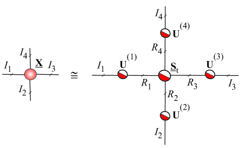
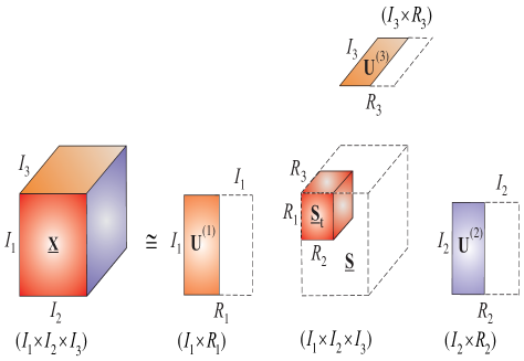
Figure  18: Graphical illustration of the HOSVD. (a) The exact HOSVD and truncated (approximative) HOSVD a for 3rd-order tensor as: 𝐗¯𝐒¯t×1𝐔(1)×2𝐔(2)×3𝐔(3)¯𝐗subscript3subscript2subscript1subscript¯𝐒𝑡superscript𝐔1superscript𝐔2superscript𝐔3\underline{{\bf X}}\cong\underline{{\bf S}}_{t}\times_{1}{\bf U}^{(1)}\times_{2}{\bf U}^{(2)}\times_{3}{\bf U}^{(3)} using a truncated SVD. (b) Tensor network notation for the HOSVD for a 4th-order tensor 𝐗¯𝐒¯t×1𝐔(1)×2𝐔(2)×3𝐔(3)×4𝐔(4)¯𝐗subscript4subscript3subscript2subscript1subscript¯𝐒𝑡superscript𝐔1superscript𝐔2superscript𝐔3superscript𝐔4\underline{{\bf X}}\cong\underline{{\bf S}}_{t}\times_{1}{\bf U}^{(1)}\times_{2}{\bf U}^{(2)}\times_{3}{\bf U}^{(3)}\times_{4}{\bf U}^{(4)}. All factor matrices 𝐔(n)superscript𝐔𝑛{\bf U}^{(n)} and the core tensor 𝐒¯tsubscript¯𝐒𝑡\underline{{\bf S}}_{t} are orthogonal; due to orthogonality of the core tensor the HOSVD is unique for a specific multilinear rank.

VI Multilinear SVD (MLSVD) for Large Scale Problems

MultiLinear Singular Value Decomposition (MLSVD), called also higher-order SVD (HOSVD) can be considered as a special form of the Tucker decomposition [43, 44], in which all factor matrices 𝐁(n)=𝐔(n)In×Imsuperscript𝐁𝑛superscript𝐔𝑛superscriptsubscript𝐼𝑛subscript𝐼𝑚{\bf B}^{(n)}={\bf U}^{(n)}\in\mathbb{R}^{I_{n}\times I_{m}} are orthogonal and the core tensor 𝐆¯=𝐒¯I1×I2××IN¯𝐆¯𝐒superscriptsubscript𝐼1subscript𝐼2subscript𝐼𝑁\underline{{\bf G}}=\underline{{\bf S}}\in\mathbb{R}^{I_{1}\times I_{2}\times\cdots\times I_{N}} is all-orthogonal (see Fig. 18).

We say that the core tensor is all-orthogonal if it satisfies the following conditions:

(1) All orthogonality: Slices in each mode are mutually orthogonal, e.g., for a 3rd-order tensor

𝐒:,k,:𝐒:,l,:=0,forkl,formulae-sequencedelimited-⟨⟩subscript𝐒:𝑘:subscript𝐒:𝑙:0for𝑘𝑙\displaystyle\langle{\bf S}_{:,k,:}{\bf S}_{:,l,:}\rangle=0,\quad\mbox{for}\quad k\neq l, (17)

(2) Pseudo-diagonality: Frobenius norms of slices in each mode are decreasing with the increase of the running index

𝐒:,k,:F𝐒:,l,:F,kl.formulae-sequencesubscriptnormsubscript𝐒:𝑘:𝐹subscriptnormsubscript𝐒:𝑙:𝐹𝑘𝑙\displaystyle||{\bf S}_{:,k,:}||_{F}\geq||{\bf S}_{:,l,:}||_{F},\quad k\geq l. (18)

These norms play a role similar to that of the singular values in the matrix SVD.

The orthogonal matrices 𝐔(n)superscript𝐔𝑛{\bf U}^{(n)} can be in practice computed by the standard SVD or truncated SVD of unfolded mode-n𝑛n matrices 𝐗(n)=𝐔(n)𝚺n𝐕(n)TIn×I1In1In+1INsubscript𝐗𝑛superscript𝐔𝑛subscript𝚺𝑛superscript𝐕𝑛𝑇superscriptsubscript𝐼𝑛subscript𝐼1subscript𝐼𝑛1subscript𝐼𝑛1subscript𝐼𝑁{\bf X}_{(n)}={\bf U}^{(n)}\mbox{\boldmath$\Sigma$}_{n}{\bf V}^{(n)T}\in\mathbb{R}^{I_{n}\times I_{1}\cdots I_{n-1}I_{n+1}\cdots I_{N}}. After obtaining the orthogonal matrices 𝐔(n)superscript𝐔𝑛{\bf U}^{(n)} of left singular vectors of 𝐗(n)subscript𝐗𝑛{\bf X}_{(n)}, for each n𝑛n, we can compute the core tensor 𝐆¯=𝐒¯¯𝐆¯𝐒\underline{{\bf G}}=\underline{{\bf S}} as

𝐒¯=𝐗¯×1𝐔(1)T×2𝐔(2)T×N𝐔(N)T,¯𝐒subscript𝑁subscript2subscript1¯𝐗superscript𝐔1𝑇superscript𝐔2𝑇superscript𝐔𝑁𝑇\displaystyle\underline{{\bf S}}=\underline{{\bf X}}\times_{1}{\bf U}^{(1)\;T}\times_{2}{\bf U}^{(2)\;T}\cdots\times_{N}{\bf U}^{(N)\;T}, (19)

such that

𝐗¯=𝐒¯×1𝐔(1)×2𝐔(2)×N𝐔(N).¯𝐗subscript𝑁subscript2subscript1¯𝐒superscript𝐔1superscript𝐔2superscript𝐔𝑁\displaystyle\underline{{\bf X}}=\underline{{\bf S}}\times_{1}{\bf U}^{(1)}\times_{2}{\bf U}^{(2)}\cdots\times_{N}{\bf U}^{(N)}. (20)

Due to orthogonality of the core tensor 𝐒¯¯𝐒\underline{{\bf S}} its slices are mutually orthogonal, this reduces to the diagonality in the matrix case.

In some applications we may use a modified HOSVD in which the SVD can be performed not on the unfolding mode-n𝑛n matrices 𝐗(n)subscript𝐗𝑛{\bf X}_{(n)} but on their transposes, i.e., 𝐗(n)T𝐕(n)𝚺n𝐔(n)Tsuperscriptsubscript𝐗𝑛𝑇superscript𝐕𝑛subscript𝚺𝑛superscript𝐔𝑛𝑇{\bf X}_{(n)}^{T}\cong{\bf V}^{(n)}\mbox{\boldmath$\Sigma$}_{n}{\bf U}^{(n)T}. This leads to the modified HOSVD corresponding to Grassmann manifolds [45], that requires the computation of very large (tall-and-skinny) factor orthogonal matrices 𝐕(n)In¯×Insuperscript𝐕𝑛superscriptsubscript𝐼¯𝑛subscript𝐼𝑛{\bf V}^{(n)}\in\mathbb{R}^{I_{\bar{n}}\times I_{n}}, where In¯=knIk=I1In1In+1INsubscript𝐼¯𝑛subscriptproduct𝑘𝑛subscript𝐼𝑘subscript𝐼1subscript𝐼𝑛1subscript𝐼𝑛1subscript𝐼𝑁I_{\bar{n}}=\prod_{k\neq n}I_{k}=I_{1}\cdots I_{n-1}I_{n+1}\cdots I_{N}, and the core tensor 𝐒¯~I1¯×I2¯××IN¯¯~𝐒superscriptsubscript𝐼¯1subscript𝐼¯2subscript𝐼¯𝑁\underline{\tilde{\bf S}}\in\mathbb{R}^{I_{\bar{1}}\times I_{\bar{2}}\times\cdots\times I_{\bar{N}}} based on the following model:

𝐗¯=𝐒¯~×1𝐕(1)T×2𝐕(2)T×N𝐕(N)T.¯𝐗subscript𝑁subscript2subscript1¯~𝐒superscript𝐕1𝑇superscript𝐕2𝑇superscript𝐕𝑁𝑇\displaystyle\underline{{\bf X}}=\underline{\tilde{\bf S}}\times_{1}{\bf V}^{(1)\;T}\times_{2}{\bf V}^{(2)\;T}\cdots\times_{N}{\bf V}^{(N)\;T}. (21)

(a) Sequential computation
Refer to caption
(b) Distributed computation
Refer to caption

(c) Divide-and-conquer approach
Refer to caption

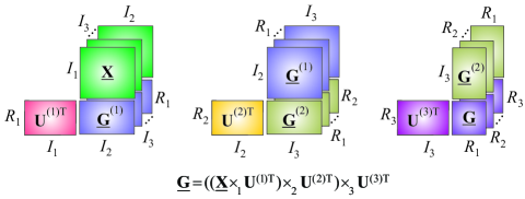
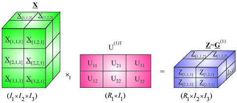
Figure  19: Computation of a core tensor for a large-scale HOSVD: (a) using sequential computing of multilinear products 𝐆¯=𝐒¯=(((𝐗¯×1𝐔(1)T)×2𝐔(2)T)×3𝐔(3)T)¯𝐆¯𝐒subscript3subscript2subscript1¯𝐗superscript𝐔1𝑇superscript𝐔2𝑇superscript𝐔3𝑇\underline{{\bf G}}=\underline{{\bf S}}=(((\underline{{\bf X}}\times_{1}{\bf U}^{(1)T})\times_{2}{\bf U}^{(2)T})\times_{3}{\bf U}^{(3)T}), and (b) by applying fast and distributed implementation of matrix by matrix multiplications; (c) alternative method for very large-scale problems by applying divide and conquer approach, in which a data tensor 𝐗¯¯𝐗\underline{{\bf X}} and factor matrices 𝐔(n)Tsuperscript𝐔𝑛𝑇{\bf U}^{(n)T} are partitioned into suitable small blocks: Subtensors 𝐗¯[k1,k2,k3]subscript¯𝐗subscript𝑘1subscript𝑘2subscript𝑘3\underline{{\bf X}}_{[k_{1},k_{2},k_{3}]} and blocks matrices 𝐔[k1,p1](1)Tsubscriptsuperscript𝐔1𝑇subscript𝑘1subscript𝑝1{\bf U}^{(1)T}_{[k_{1},p_{1}]}, respectively. We compute the blocks of tensor 𝐙¯=𝐆¯(1)=𝐗¯×1𝐔(1)T¯𝐙superscript¯𝐆1subscript1¯𝐗superscript𝐔1𝑇\underline{{\bf Z}}=\underline{{\bf G}}^{(1)}=\underline{{\bf X}}\times_{1}{\bf U}^{(1)T} as follows 𝐙¯[q1,k2,k3]=k1=1K1𝐗[k1,k2,k3]×1𝐔[k1,q1](1)Tsubscript¯𝐙subscript𝑞1subscript𝑘2subscript𝑘3superscriptsubscriptsubscript𝑘11subscript𝐾1subscript1subscript𝐗subscript𝑘1subscript𝑘2subscript𝑘3subscriptsuperscript𝐔1𝑇subscript𝑘1subscript𝑞1\underline{{\bf Z}}_{[q_{1},k_{2},k_{3}]}=\sum_{k_{1}=1}^{K_{1}}{\bf X}_{[k_{1},k_{2},k_{3}]}\times_{1}{\bf U}^{(1)T}_{[k_{1},q_{1}]} (see Eq. (23) for a general case.)
Refer to caption
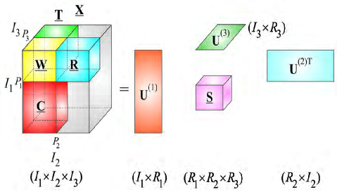
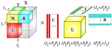
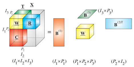
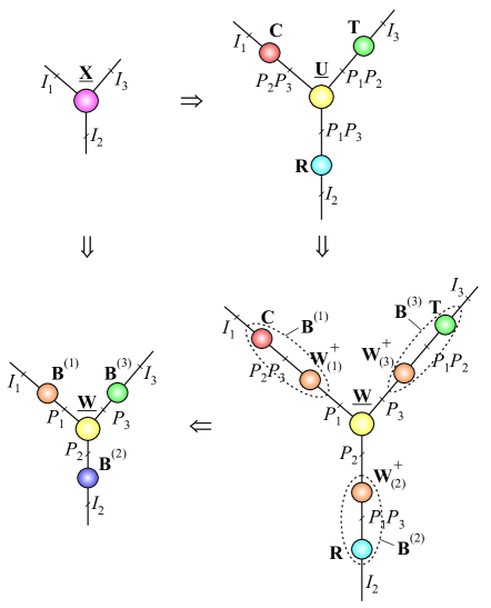
Figure  20: Alternative approach to computation of the HOSVD for very large data tensor, by exploiting multilinear low-rank approximation. The objective is to select such fibers (up to permutation of fibers) that the subtensor 𝐖¯P1×P2×P3¯𝐖superscriptsubscript𝑃1subscript𝑃2subscript𝑃3\underline{{\bf W}}\in\mathbb{R}^{P_{1}\times P_{2}\times P_{3}} with PnRnsubscript𝑃𝑛subscript𝑅𝑛P_{n}\geq R_{n} (n=1,2,3𝑛123n=1,2,3) has the same multilinear rank {R1,R2,R3}subscript𝑅1subscript𝑅2subscript𝑅3\{R_{1},R_{2},R_{3}\} as the whole huge data tensor 𝐗¯¯𝐗\underline{{\bf X}}, with RnInmuch-less-thansubscript𝑅𝑛subscript𝐼𝑛R_{n}\ll I_{n}. Instead of unfolding of the whole data tensor 𝐗¯¯𝐗\underline{{\bf X}} we need to perform unfolding (and applying the standard SVD) for typically much smaller subtensors 𝐗¯(1)=𝐂¯I1×P2×P3,𝐗¯(2)=𝐑¯P1×I2×P3,𝐗¯(3)=𝐓¯P1×P2×I3formulae-sequencesuperscript¯𝐗1¯𝐂superscriptsubscript𝐼1subscript𝑃2subscript𝑃3superscript¯𝐗2¯𝐑superscriptsubscript𝑃1subscript𝐼2subscript𝑃3superscript¯𝐗3¯𝐓superscriptsubscript𝑃1subscript𝑃2subscript𝐼3\underline{{\bf X}}^{(1)}=\underline{{\bf C}}\in\mathbb{R}^{I_{1}\times P_{2}\times P_{3}},\;\underline{{\bf X}}^{(2)}=\underline{{\bf R}}\in\mathbb{R}^{P_{1}\times I_{2}\times P_{3}},\;\underline{{\bf X}}^{(3)}=\underline{{\bf T}}\in\mathbb{R}^{P_{1}\times P_{2}\times I_{3}}, each in a single mode-n𝑛n, (n=1,2,3𝑛123n=1,2,3). This approach can be applied if data tensor admits low multilinear rank approximation. For simplicity of illustration, we assumed that fibers are permuted in a such way that the first P1,P2,P3𝑃1subscript𝑃2subscript𝑃3P-1,P_{2},P_{3} fibers were selected.

In practical applications the dimensions of unfolding matrices 𝐗(n)In×In¯subscript𝐗𝑛superscriptsubscript𝐼𝑛subscript𝐼¯𝑛{\bf X}_{(n)}\in\mathbb{R}^{I_{n}\times I_{\bar{n}}} may be prohibitively large (with In¯Inmuch-greater-thansubscript𝐼¯𝑛subscript𝐼𝑛I_{\bar{n}}\gg I_{n}), easily exceeding memory of standard computers. A truncated SVD of a large-scale unfolding matrix 𝐗(n)=𝐔(n)𝚺n𝐕(n)Tsubscript𝐗𝑛superscript𝐔𝑛subscript𝚺𝑛superscript𝐕𝑛𝑇\mathbf{X}_{(n)}={\bf U}^{(n)}\mathbf{\Sigma}_{n}{\bf V}^{(n)T} is performed by partitioning it into Q𝑄Q slices, as 𝐗(n)=[𝐗1,n,𝐗2,n,,𝐗Q,n]=𝐔(n)𝚺n[𝐕1,nT,𝐕2,nT,,𝐕Q,nT]subscript𝐗𝑛subscript𝐗1𝑛subscript𝐗2𝑛subscript𝐗𝑄𝑛superscript𝐔𝑛subscript𝚺𝑛superscriptsubscript𝐕1𝑛𝑇superscriptsubscript𝐕2𝑛𝑇superscriptsubscript𝐕𝑄𝑛𝑇\mathbf{X}_{(n)}=[\mathbf{X}_{1,n},\mathbf{X}_{2,n},\ldots,\mathbf{X}_{Q,n}]={\bf U}^{(n)}\mathbf{\Sigma}_{n}[\mathbf{V}_{1,n}^{T},\mathbf{V}_{2,n}^{T},\ldots,\mathbf{V}_{Q,n}^{T}]. Next, the orthogonal matrices 𝐔(n)superscript𝐔𝑛{\bf U}^{(n)} and the diagonal matrices 𝚺nsubscript𝚺𝑛\mathbf{\Sigma}_{n} are obtained from eigenvalue decompositions 𝐗(n)𝐗(n)T=𝐔(n)𝚺n2𝐔(n)T=q𝐗q,n𝐗q,nTIn×Insubscript𝐗𝑛superscriptsubscript𝐗𝑛𝑇superscript𝐔𝑛superscriptsubscript𝚺𝑛2superscript𝐔𝑛𝑇subscript𝑞subscript𝐗𝑞𝑛superscriptsubscript𝐗𝑞𝑛𝑇superscriptsubscript𝐼𝑛subscript𝐼𝑛\mathbf{X}_{(n)}\mathbf{X}_{(n)}^{T}={\bf U}^{(n)}\mathbf{\Sigma}_{n}^{2}{\bf U}^{(n)T}=\sum_{q}\mathbf{X}_{q,n}\mathbf{X}_{q,n}^{T}\in\mathbb{R}^{I_{n}\times I_{n}}, allowing for the terms 𝐕q,n=𝐗q,nT𝐔(n)𝚺n1subscript𝐕𝑞𝑛superscriptsubscript𝐗𝑞𝑛𝑇superscript𝐔𝑛superscriptsubscript𝚺𝑛1\mathbf{V}_{q,n}=\mathbf{X}_{q,n}^{T}{\bf U}^{(n)}\mathbf{\Sigma}_{n}^{-1} to be computed separately. This allows us to optimize the size of the q𝑞q-th slice 𝐗q,nIn×(In¯/Q)subscript𝐗𝑞𝑛superscriptsubscript𝐼𝑛subscript𝐼¯𝑛𝑄{\bf X}_{q,n}\in\mathbb{R}^{I_{n}\times(I_{\bar{n}}/Q)} so as to match the available computer memory. Such a simple approach to compute matrices 𝐔(n)superscript𝐔𝑛{\bf U}^{(n)} and/or 𝐕(n)superscript𝐕𝑛{\bf V}^{(n)} does not require loading the entire unfolding matrices at once into computer memory, instead the access to the dataset is sequential. Depending on the size of computer memory, the dimension Insubscript𝐼𝑛I_{n} is typically less than 10,000, while there is no limit on the dimension In¯=knIksubscript𝐼¯𝑛subscriptproduct𝑘𝑛subscript𝐼𝑘I_{\bar{n}}=\prod_{k\neq n}I_{k}. More sophisticated approaches which also exploit partition of matrices or tensors into blocks for QR/SVD, PCA, NMF/NTF and ICA can be found in [46, 47, 48, 10, 29].

When a data tensor 𝐗¯¯𝐗\underline{{\bf X}} is very large and cannot be stored in computer memory, then another challenge is to compute a core tensor 𝐆¯=𝐒¯¯𝐆¯𝐒\underline{{\bf G}}=\underline{{\bf S}} by directly using the formula:

𝐆=𝐗¯×1𝐔(1)T×2𝐔(2)T×n𝐔(n)T,𝐆subscript𝑛subscript2subscript1¯𝐗superscript𝐔1𝑇superscript𝐔2𝑇superscript𝐔𝑛𝑇\displaystyle{\bf G}=\underline{{\bf X}}\times_{1}{\bf U}^{(1)T}\times_{2}{\bf U}^{(2)T}\cdots\times_{n}{\bf U}^{(n)T}, (22)

which is generally performed sequentially as illustrated in Fig. 19 (a) and (b) [8, 9].

For very large tensors it is useful to divide the data tensor 𝐗¯¯𝐗\underline{{\bf X}} into small blocks 𝐗¯[k1,k2,,kN]subscript¯𝐗subscript𝑘1subscript𝑘2subscript𝑘𝑁\underline{{\bf X}}_{[k_{1},k_{2},\ldots,k_{N}]} and in order to store them on hard disks or distributed memory. In similar way, we can divide the orthogonal factor matrices 𝐔(n)Tsuperscript𝐔𝑛𝑇{\bf U}^{(n)T} into corresponding blocks of matrices 𝐔[kn,pn](n)Tsubscriptsuperscript𝐔𝑛𝑇subscript𝑘𝑛subscript𝑝𝑛{\bf U}^{(n)T}_{[k_{n},p_{n}]} as illustrated in Fig. 19 (c) for 3rd-order tensors [9]. In a general case, we can compute blocks within the resulting tensor 𝐆(n)superscript𝐆𝑛{\bf G}^{(n)} sequentially or in parallel way as follows:

𝐆¯[k1,k2,,qn,,kN](n)=kn=1Kn𝐗[k1,k2,,kn,,kN]×n𝐔[kn,qn](n)T.subscriptsuperscript¯𝐆𝑛subscript𝑘1subscript𝑘2subscript𝑞𝑛subscript𝑘𝑁superscriptsubscriptsubscript𝑘𝑛1subscript𝐾𝑛subscript𝑛subscript𝐗subscript𝑘1subscript𝑘2subscript𝑘𝑛subscript𝑘𝑁subscriptsuperscript𝐔𝑛𝑇subscript𝑘𝑛subscript𝑞𝑛\displaystyle\underline{{\bf G}}^{(n)}_{[k_{1},k_{2},\ldots,q_{n},\ldots,k_{N}]}=\sum_{k_{n}=1}^{K_{n}}{\bf X}_{[k_{1},k_{2},\ldots,k_{n},\ldots,k_{N}]}\times_{n}{\bf U}^{(n)\;T}_{[k_{n},q_{n}]}. (23)

If a data tensor has low-multilinear rank, so that its multilinear rank {R1,R2,,RN}subscript𝑅1subscript𝑅2subscript𝑅𝑁\{R_{1},R_{2},\ldots,R_{N}\} with RnIn,nmuch-less-thansubscript𝑅𝑛subscript𝐼𝑛for-all𝑛R_{n}\ll I_{n},\;\;\forall n, we can further alleviate the problem of dimensionality by first identifying a subtensor 𝐖¯P1×P2×PN¯𝐖superscriptsubscript𝑃1subscript𝑃2subscript𝑃𝑁\underline{{\bf W}}\in\mathbb{R}^{P_{1}\times P_{2}\times\cdots P_{N}} for which PnRnsubscript𝑃𝑛subscript𝑅𝑛P_{n}\geq R_{n}, using efficient CUR tensor decompositions [49]. Then the HOSVD can be computed from subtensors as illustrated in Fig. 20 for a 3rd-order tensor. This feature can be formulated in more general form as the following Proposition.

Proposition 1: If a tensor 𝐗¯I1×I2××IN¯𝐗superscriptsubscript𝐼1subscript𝐼2subscript𝐼𝑁\underline{{\bf X}}\in\mathbb{R}^{I_{1}\times I_{2}\times\cdots\times I_{N}} has low multilinear rank {R1,R2,,RN}subscript𝑅1subscript𝑅2subscript𝑅𝑁\{R_{1},R_{2},\ldots,R_{N}\}, with RnIn,nsubscript𝑅𝑛subscript𝐼𝑛for-all𝑛R_{n}\leq I_{n},\;\;\forall n, then it can be fully reconstructed via the HOSVD using only N𝑁N subtensors 𝐗¯(n)P1××Pn1×In×Pn+1××PN,(n=1,2,,N)superscript¯𝐗𝑛superscriptsubscript𝑃1subscript𝑃𝑛1subscript𝐼𝑛subscript𝑃𝑛1subscript𝑃𝑁𝑛12𝑁\underline{{\bf X}}^{(n)}\in\mathbb{R}^{P_{1}\times\cdots\times P_{n-1}\times I_{n}\times P_{n+1}\times\cdots\times P_{N}},\;\ (n=1,2,\ldots,N), under the condition that subtensor 𝐖¯P1×P2××PN¯𝐖superscriptsubscript𝑃1subscript𝑃2subscript𝑃𝑁\underline{{\bf W}}\in\mathbb{R}^{P_{1}\times P_{2}\times\cdots\times P_{N}}, with PnRn,nsubscript𝑃𝑛subscript𝑅𝑛for-all𝑛P_{n}\geq R_{n},\;\;\forall n has the multilinear rank {R1,R2,,RN}subscript𝑅1subscript𝑅2subscript𝑅𝑁\{R_{1},R_{2},\ldots,R_{N}\}.

In practice, we can compute the HOSVD for low-rank, large-scale data tensors in several steps. In the first step, we can apply the CUR FSTD decomposition [49] to identify close to optimal a subtensor 𝐖¯R1×R2××RN¯𝐖superscriptsubscript𝑅1subscript𝑅2subscript𝑅𝑁\underline{{\bf W}}\in\mathbb{R}^{R_{1}\times R_{2}\times\cdots\times R_{N}} (see the next Section), In the next step, we can use the standard SVD for unfolding matrices 𝐗(n)(n)subscriptsuperscript𝐗𝑛𝑛{\bf X}^{(n)}_{(n)} of subtensors 𝐗¯(n)superscript¯𝐗𝑛\underline{{\bf X}}^{(n)} to compute the left orthogonal matrices 𝐔~(n)In×Rnsuperscript~𝐔𝑛superscriptsubscript𝐼𝑛subscript𝑅𝑛\widetilde{\bf U}^{(n)}\in\mathbb{R}^{I_{n}\times R_{n}}. Hence, we compute an auxiliary core tensor 𝐆¯=𝐖¯×1𝐁(1)×N𝐁(N)¯𝐆subscript𝑁subscript1¯𝐖superscript𝐁1superscript𝐁𝑁\underline{{\bf G}}=\underline{{\bf W}}\times_{1}{\bf B}^{(1)}\cdots\times_{N}{\bf B}^{(N)}, where 𝐁(n)Rn×Rnsuperscript𝐁𝑛superscriptsubscript𝑅𝑛subscript𝑅𝑛{\bf B}^{(n)}\in\mathbb{R}^{R_{n}\times R_{n}} are inverses of the sub-matrices consisting the first Rnsubscript𝑅𝑛R_{n} rows of the matrices 𝐔~(n)superscript~𝐔𝑛\widetilde{\bf U}^{(n)}. In the last step, we perform HOSVD decomposition of the relatively small core tensor as 𝐆¯=𝐒¯×1𝐐(1)×N𝐐(N)¯𝐆subscript𝑁subscript1¯𝐒superscript𝐐1superscript𝐐𝑁\underline{{\bf G}}=\underline{{\bf S}}\times_{1}{\bf Q}^{(1)}\cdots\times_{N}{\bf Q}^{(N)}, with 𝐐(n)Rn×Rnsuperscript𝐐𝑛superscriptsubscript𝑅𝑛subscript𝑅𝑛{\bf Q}^{(n)}\in\mathbb{R}^{R_{n}\times R_{n}} and then desired orthogonal matrices are computed as 𝐔(n)=𝐔~(n)𝐐(n)superscript𝐔𝑛superscript~𝐔𝑛superscript𝐐𝑛{\bf U}^{(n)}=\widetilde{\bf U}^{(n)}{\bf Q}^{(n)}.

VII CUR Tucker Decomposition for Dimensionality Reduction and Compression of Tensor Data

Note that instead of using the full tensor, we may compute an approximative tensor decomposition model from a limited number of entries (e.g., selected fibers, slices or subtensors). Such completion-type strategies have been developed for low-rank and low-multilinear-rank [50, 51]. A simple approach would be to apply CUR decomposition or Cross-Approximation by sampled fibers for the columns of factor matrices in a Tucker approximation [52, 49]. Another approach is to apply tensor networks to represent big data by high-order tensors not explicitly but in compressed tensor formats (see next sections). Dimensionality reduction methods are based on the fundamental assumption that large datasets are highly redundant and can be approximated by low-rank matrices and cores, allowing for a significant reduction in computational complexity and to discover meaningful components while exhibiting marginal loss of information.

For very large-scale matrices, the so called CUR matrix decompositions can be employed for dimensionality reduction [53, 54, 52, 49, 55]. Assuming a sufficiently precise low-rank approximation, which implies that data has some internal structure or smoothness, the idea is to provide data representation through a linear combination of a few “meaningful” components, which are exact replicas of columns and rows of the original data matrix [56].
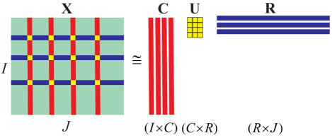
Refer to caption
Figure  21: CUR decomposition for a huge matrix.

(a)
Refer to caption

(b)
Refer to caption

(c)
Refer to caption

Figure  22: (a) CUR decomposition of a large 3rd-order tensor (for simplicity of illustration up to permutation of fibers) 𝐗¯𝐔¯×1𝐂×2𝐑×3𝐓=𝐔¯;𝐂,𝐑,𝐓¯𝐗subscript3subscript2subscript1¯𝐔𝐂𝐑𝐓¯𝐔𝐂𝐑𝐓\underline{{\bf X}}\cong\underline{{\bf U}}\times_{1}{\bf C}\times_{2}{\bf R}\times_{3}{\bf T}=\llbracket\underline{{\bf U}};{\bf C},{\bf R},{\bf T}\rrbracket, where 𝐔¯=𝐖¯×1𝐖(1)×2𝐖(2)×3𝐖(3)=𝐖¯;𝐖(1),𝐖(2),𝐖(3)¯𝐔subscript3subscript2subscript1¯𝐖superscriptsubscript𝐖1superscriptsubscript𝐖2superscriptsubscript𝐖3¯𝐖superscriptsubscript𝐖1superscriptsubscript𝐖2superscriptsubscript𝐖3\underline{{\bf U}}=\underline{{\bf W}}\times_{1}\mathbf{W}_{(1)}^{\dagger}\times_{2}\mathbf{W}_{(2)}^{\dagger}\times_{3}\mathbf{W}_{(3)}^{\dagger}=\llbracket\underline{{\bf W}};\mathbf{W}_{(1)}^{\dagger},\mathbf{W}_{(2)}^{\dagger},\mathbf{W}_{(3)}^{\dagger}\rrbracket. (b) equivalent decomposition expressed via subtensor 𝐖¯¯𝐖\underline{{\bf W}}, (c) Tensor network diagram illustrating transformation from CUR Tucker format (a) to form (b) as: 𝐗¯𝐖¯×1𝐁(1)×2𝐁(2)×3𝐁(3)=𝐖¯;𝐂𝐖(1),𝐑𝐖(2),𝐓𝐖(3)¯𝐗subscript3subscript2subscript1¯𝐖superscript𝐁1superscript𝐁2superscript𝐁3¯𝐖superscriptsubscript𝐂𝐖1superscriptsubscript𝐑𝐖2superscriptsubscript𝐓𝐖3\underline{{\bf X}}\cong\underline{{\bf W}}\times_{1}{\bf B}^{(1)}\times_{2}{\bf B}^{(2)}\times_{3}{\bf B}^{(3)}=\llbracket\underline{{\bf W}};{\bf C}{\bf W}_{(1)}^{\dagger},{\bf R}{\bf W}_{(2)}^{\dagger},{\bf T}{\bf W}_{(3)}^{\dagger}\rrbracket.

The CUR model, also called skeleton Cross-Approximation, decomposes a data matrix 𝐗I×J𝐗superscript𝐼𝐽{\bf X}\in\mathbb{R}^{I\times J} as [53, 54] (see Fig. 21):

𝐗=𝐂𝐔𝐑+𝐄,𝐗𝐂𝐔𝐑𝐄\displaystyle{\bf X}={\bf C}{\bf U}{\bf R}+{\bf E}, (24)

where 𝐂I×C𝐂superscript𝐼𝐶{\bf C}\in\mathbb{R}^{I\times C} is a matrix constructed from C𝐶C suitably selected columns of the data matrix 𝐗𝐗{\bf X}, 𝐑R×J𝐑superscript𝑅𝐽{\bf R}\in\mathbb{R}^{R\times J} consists of R𝑅R rows of 𝐗𝐗{\bf X}, and the matrix 𝐔C×R𝐔superscript𝐶𝑅{\bf U}\in\mathbb{R}^{C\times R} is chosen to minimize the norm of the error 𝐄I×J𝐄superscript𝐼𝐽{\bf E}\in\mathbb{R}^{I\times J}. Since typically, CJmuch-less-than𝐶𝐽C\ll J and RImuch-less-than𝑅𝐼R\ll I, these columns and rows are chosen so as to exhibit high “statistical leverage” and provide the best low-rank fit to the data matrix, at the same time the error cost function 𝐄F2superscriptsubscriptnorm𝐄𝐹2||{\bf E}||_{F}^{2} is minimized. For a given set of columns (𝐂𝐂{\bf C}) and rows (𝐑𝐑{\bf R}), the optimal choice for the core matrix is 𝐔=𝐂𝐗(𝐑)T𝐔superscript𝐂𝐗superscriptsuperscript𝐑𝑇{\bf U}={\bf C}^{\dagger}{\bf X}({\bf R}^{\dagger})^{T}. This requires access to all the entries of 𝐗𝐗{\bf X} and is not practical or feasible for large-scale data. A pragmatic choice for the core matrix would be 𝐔=𝐖𝐔superscript𝐖{\bf U}={\bf W}^{\dagger}, where the matrix 𝐖R×C𝐖superscript𝑅𝐶{\bf W}\in\mathbb{R}^{R\times C} is defined from the intersections of the selected rows and columns. It should be noted that, if rank(𝐗)C,R𝐗𝐶𝑅({\bf X})\leq C,R, then the CUR approximation is exact. For the general case, it has been proven that, when the intersection sub-matrix 𝐖𝐖{\bf W} is of maximum volume (the volume of a sub-matrix 𝐖𝐖{\bf W} is defined as |det(𝐖)|𝐖|\det({\bf W})|), this approximation is close to the optimal SVD solution [54].

The concept of CUR decomposition has been successfully generalized to tensors. In [52] the matrix CUR decomposition was applied to one unfolded version of the tensor data, while in [49] a reconstruction formula of a tensor having a low rank Tucker approximation was proposed, termed the Fiber Sampling Tucker Decomposition (FSTD), which is a practical and fast technique. The FSTD takes into account the linear structure in all the modes of the tensor simultaneously. Since real-life data often have good low multilinear rank approximations, the FSTD provides such a low-rank Tucker decomposition that is directly expressed in terms of a relatively small number of fibers of the data tensor (see Fig. 22).

For a given 3rd-order tensor 𝐗¯I1×I2×I3¯𝐗superscriptsubscript𝐼1subscript𝐼2subscript𝐼3\underline{{\bf X}}\in\mathbb{R}^{I_{1}\times I_{2}\times I_{3}} for which an exact rank-(R1,R2,R3)subscript𝑅1subscript𝑅2subscript𝑅3(R_{1},R_{2},R_{3}) Tucker representation exists, FSTD selects PnRnsubscript𝑃𝑛subscript𝑅𝑛P_{n}\geq R_{n} (n=1,2,3𝑛123n=1,2,3) indices in each mode, which determine an intersection sub-tensor 𝐖¯P1×P2×P3¯𝐖superscriptsubscript𝑃1subscript𝑃2subscript𝑃3\underline{{\bf W}}\in\mathbb{R}^{P_{1}\times P_{2}\times P_{3}} so that the following exact Tucker representation can be obtained:

𝐗¯=𝐔¯;𝐂,𝐑,𝐓,¯𝐗¯𝐔𝐂𝐑𝐓\underline{{\bf X}}=\llbracket\underline{{\bf U}};{\bf C},{\bf R},{\bf T}\rrbracket, (25)

in which the core tensor is computed as 𝐔¯=𝐆¯=𝐖¯;𝐖(1),𝐖(2),𝐖(3)¯𝐔¯𝐆¯𝐖superscriptsubscript𝐖1superscriptsubscript𝐖2superscriptsubscript𝐖3\underline{{\bf U}}=\underline{{\bf G}}=\llbracket\underline{{\bf W}};\mathbf{W}_{(1)}^{\dagger},\mathbf{W}_{(2)}^{\dagger},\mathbf{W}_{(3)}^{\dagger}\rrbracket, and the factor matrices 𝐂I1×P2P3,𝐑I2×P1P3,𝐓I3×P1P2formulae-sequence𝐂superscriptsubscript𝐼1subscript𝑃2subscript𝑃3formulae-sequence𝐑superscriptsubscript𝐼2subscript𝑃1subscript𝑃3𝐓superscriptsubscript𝐼3subscript𝑃1subscript𝑃2{\bf C}\in\mathbb{R}^{I_{1}\times P_{2}P_{3}},{\bf R}\in\mathbb{R}^{I_{2}\times P_{1}P_{3}},{\bf T}\in\mathbb{R}^{I_{3}\times P_{1}P_{2}} contain the fibers (columns, rows and tubes, respectively). This can also be written as a Tucker representation:

𝐗¯=𝐖¯;𝐂𝐖(1),𝐑𝐖(2),𝐓𝐖(3).¯𝐗¯𝐖superscriptsubscript𝐂𝐖1superscriptsubscript𝐑𝐖2superscriptsubscript𝐓𝐖3\underline{{\bf X}}=\llbracket\underline{{\bf W}};\mathbf{C}\mathbf{W}_{(1)}^{\dagger},\mathbf{R}\mathbf{W}_{(2)}^{\dagger},\mathbf{T}\mathbf{W}_{(3)}^{\dagger}\rrbracket. (26)

Observe that for N=2𝑁2N=2 this model simplifies into the CUR matrix case, 𝐗=𝐂𝐔𝐑𝐗𝐂𝐔𝐑{\bf X}={\bf C}{\bf U}{\bf R}, and the core matrix is 𝐔=𝐖;𝐖(1),𝐖(2)=𝐖𝐖𝐖=𝐖𝐔𝐖superscriptsubscript𝐖1superscriptsubscript𝐖2superscript𝐖superscript𝐖𝐖superscript𝐖\mathbf{U}=\llbracket\mathbf{W};\mathbf{W}_{(1)}^{\dagger},\mathbf{W}_{(2)}^{\dagger}\rrbracket=\mathbf{W}^{\dagger}\mathbf{W}\mathbf{W}^{\dagger}=\mathbf{W}^{\dagger}.

In a more general case for an N𝑁Nth-order tensor, we can formulate the following Proposition [49].

Proposition 2: If tensor 𝐗¯I1×I2××IN¯𝐗superscriptsubscript𝐼1subscript𝐼2subscript𝐼𝑁\underline{{\bf X}}\in\mathbb{R}^{I_{1}\times I_{2}\times\cdots\times I_{N}} has low multilinear rank {R1,R2,,RN}subscript𝑅1subscript𝑅2subscript𝑅𝑁\{R_{1},R_{2},\ldots,R_{N}\}, with RnIn,nsubscript𝑅𝑛subscript𝐼𝑛for-all𝑛R_{n}\leq I_{n},\;\;\forall n, then it can be fully reconstructed via the CUR FSTD 𝐗¯=𝐔¯;𝐂(1),𝐂(2),,𝐂(N)¯𝐗¯𝐔superscript𝐂1superscript𝐂2superscript𝐂𝑁\underline{{\bf X}}=\llbracket\underline{{\bf U}};{\bf C}^{(1)},{\bf C}^{(2)},\ldots,{\bf C}^{(N)}\rrbracket, using only N𝑁N factor matrices 𝐂(n)In×Pn,(n=1,2,,N)superscript𝐂𝑛superscriptsubscript𝐼𝑛subscript𝑃𝑛𝑛12𝑁{\bf C}^{(n)}\in\mathbb{R}^{I_{n}\times P_{n}},\;\ (n=1,2,\ldots,N), built up from fibers of the data tensor, and a core tensor 𝐔¯=𝐆¯=𝐖¯;𝐖(1),𝐖(2),,𝐖(N)¯𝐔¯𝐆¯𝐖superscriptsubscript𝐖1superscriptsubscript𝐖2superscriptsubscript𝐖𝑁\underline{{\bf U}}=\underline{{\bf G}}=\llbracket\underline{{\bf W}};\mathbf{W}_{(1)}^{\dagger},\mathbf{W}_{(2)}^{\dagger},\ldots,\mathbf{W}_{(N)}^{\dagger}\rrbracket, under the condition that subtensor 𝐖¯P1×P2××PN¯𝐖superscriptsubscript𝑃1subscript𝑃2subscript𝑃𝑁\underline{{\bf W}}\in\mathbb{R}^{P_{1}\times P_{2}\times\cdots\times P_{N}} with PnRn,nsubscript𝑃𝑛subscript𝑅𝑛for-all𝑛P_{n}\geq R_{n},\;\;\forall n has multilinear rank {R1,R2,,RN}subscript𝑅1subscript𝑅2subscript𝑅𝑁\{R_{1},R_{2},\ldots,R_{N}\}).

An efficient strategy for the selection of suitable fibers, only requiring access to a partial (small) subset of entries of a data tensor through identifying the entries with maximum modulus within single fibers is given in [49]. The indices are selected sequentially using a deflation approach making the FSTD algorithm suitable for very large-scale but relatively low-order tensors (including tensors with missing fibers or entries).

VIII Analysis of Coupled Multi-Block Tensor Data – Linked Multiway Component Analysis (LMWCA)

Group analysis or multi-block data analysis aims to identify links between hidden components in data making it possible to analyze the correlation, variability and consistency of the components across multi-block data sets. This equips us with enhanced flexibility: Some components do not necessarily need to be orthogonal or statistically independent, and can be instead sparse, smooth or non-negative (e.g., for spectral components). Additional constraints can be used to reflect the spatial distributions, spectral, or temporal patterns [3].

Consider the analysis of multi-modal high-dimensional data collected under the same or very similar conditions, for example, a set of EEG and MEG or fMRI signals recorded for different subjects over many trials and under the same experiment configuration and mental tasks. Such data share some common latent (hidden) components but can also have their own independent features. Therefore, it is quite important and necessary that they will be analyzed in a linked way instead of independently.
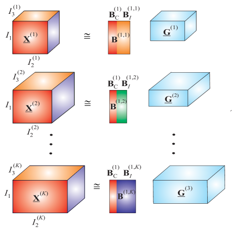
Refer to caption
Figure  23: Linked Multiway Component Analysis (LMWCA) for coupled multi-block 3rd-order tensors, with different dimensions in each mode except of the first mode. The objective is to find the common components 𝐁C(1)I1×C1subscriptsuperscript𝐁1𝐶superscriptsubscript𝐼1subscript𝐶1{\bf B}^{(1)}_{C}\in\mathbb{R}^{I_{1}\times C_{1}}, where C1R1subscript𝐶1subscript𝑅1C_{1}\leq R_{1} is the number of the common components in mode-1.

The linked multiway component analysis (LMWCA) for multi-block tensors data is formulated as a set of approximate joint Tucker-(1,N)1𝑁(1,N) decompositions of a set of data tensors 𝐗¯(k)I1(k)×I2(k)××IN(k)superscript¯𝐗𝑘superscriptsuperscriptsubscript𝐼1𝑘superscriptsubscript𝐼2𝑘superscriptsubscript𝐼𝑁𝑘\underline{{\bf X}}^{(k)}\in\mathbb{R}^{I_{1}^{(k)}\times I_{2}^{(k)}\times\cdots\times I_{N}^{(k)}}, with I1(k)=I1,ksuperscriptsubscript𝐼1𝑘subscript𝐼1for-all𝑘I_{1}^{(k)}=I_{1},\;\;\forall k (k=1,2,,K)𝑘12𝐾\;(k=1,2,\ldots,K) (see Fig. 23):

𝐗¯(k)=𝐆¯(k)×1𝐁(1,k),(k=1,2,K)superscript¯𝐗𝑘subscript1superscript¯𝐆𝑘superscript𝐁1𝑘𝑘12𝐾\displaystyle\underline{{\bf X}}^{(k)}=\underline{{\bf G}}^{(k)}\times_{1}{\bf B}^{(1,k)},\quad(k=1,2,\ldots K) (27)

where each factor (component) matrix 𝐁(1,k)=[𝐁C(1),𝐁I(1,k)]In×Rnsuperscript𝐁1𝑘subscriptsuperscript𝐁1𝐶subscriptsuperscript𝐁1𝑘𝐼superscriptsubscript𝐼𝑛subscript𝑅𝑛{\bf B}^{(1,k)}=[{\bf B}^{(1)}_{C},\;{\bf B}^{(1,k)}_{I}]\in\mathbb{R}^{I_{n}\times R_{n}} has two sets of components: (1) Components 𝐁C(1)I1×Csubscriptsuperscript𝐁1𝐶superscriptsubscript𝐼1𝐶{\bf B}^{(1)}_{C}\in\mathbb{R}^{I_{1}\times C} (with 0CR0𝐶𝑅0\leq C\leq R), which are common for all available blocks and correspond to identical or maximally correlated components, and (2) components 𝐁I(1,k)I1×(R1C1)subscriptsuperscript𝐁1𝑘𝐼superscriptsubscript𝐼1subscript𝑅1subscript𝐶1{\bf B}^{(1,k)}_{I}\in\mathbb{R}^{I_{1}\times(R_{1}-C_{1})}, which are different independent processes, for example, latent variables independent of excitations or stimuli/tasks. The objective is to estimate the common components 𝐁C(1)superscriptsubscript𝐁𝐶1{\bf B}_{C}^{(1)} and independent (distinctive) components 𝐁I(1,k)subscriptsuperscript𝐁1𝑘𝐼{\bf B}^{(1,k)}_{I} (see Fig. 23) [3].

If 𝐁(n,k)=𝐁C(n)In×Rnsuperscript𝐁𝑛𝑘subscriptsuperscript𝐁𝑛𝐶superscriptsubscript𝐼𝑛subscript𝑅𝑛{\bf B}^{(n,k)}={\bf B}^{(n)}_{C}\in\mathbb{R}^{I_{n}\times R_{n}} for a specific mode n𝑛n (in our case n=1𝑛1n=1), under additional assumption that tensors are of the same dimension. Then the problem simplifies into generalized Common Component Analysis or tensor Population Value Decomposition (PVD) [57] and can be solved by concatenating all data tensors along one mode, and perform constrained Tucker or CP tensor decompositions (see [57]).

(a)
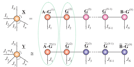
Refer to caption (b)
Refer to caption

Figure  24: Conceptual models of generalized Linked Multiway Component Analysis (LMWCA) applied to tensor networks: The objective is to find core tensors which are maximally correlated for (a) Tenor Train and for (b) Tensor Tree States (Hierarchical Tucker).

In a more general case, when Cn<Rnsubscript𝐶𝑛subscript𝑅𝑛C_{n}<R_{n}, we can unfold each data tensor 𝐗¯(k)superscript¯𝐗𝑘\underline{{\bf X}}^{(k)} in common mode, and perform a set of linked and constrained matrix factorizations: 𝐗(1)(k)𝐁C(1)𝐀C(1,k)+𝐁I(1,k)𝐀I(1,k)superscriptsubscript𝐗1𝑘subscriptsuperscript𝐁1𝐶subscriptsuperscript𝐀1𝑘𝐶subscriptsuperscript𝐁1𝑘𝐼subscriptsuperscript𝐀1𝑘𝐼{\bf X}_{(1)}^{(k)}\cong{\bf B}^{(1)}_{C}\mathbf{A}^{(1,k)}_{C}+\mathbf{B}^{(1,k)}_{I}\mathbf{A}^{(1,k)}_{I} through solving constrained optimization problems:

mink=1K𝐗(1)(k)𝐁C(1)𝐀C(1,k)𝐁I(1,k)𝐀I(1,k)F+f1(𝐁C(1)),s.t.𝐁C(1)T𝐁I(1,k)=𝟎k,formulae-sequencesuperscriptsubscript𝑘1𝐾subscriptdelimited-∥∥superscriptsubscript𝐗1𝑘subscriptsuperscript𝐁1𝐶subscriptsuperscript𝐀1𝑘𝐶subscriptsuperscript𝐁1𝑘𝐼subscriptsuperscript𝐀1𝑘𝐼𝐹subscript𝑓1subscriptsuperscript𝐁1𝐶𝑠𝑡superscriptsubscript𝐁𝐶1𝑇subscriptsuperscript𝐁1𝑘𝐼0for-all𝑘\begin{split}\min\;&\sum_{k=1}^{K}\|{\bf X}_{(1)}^{(k)}-{\bf B}^{(1)}_{C}\mathbf{A}^{(1,k)}_{C}-\mathbf{B}^{(1,k)}_{I}\mathbf{A}^{(1,k)}_{I}\|_{F}\\ &+f_{1}({\bf B}^{(1)}_{C}),\;\;s.t.\;\;{\bf B}_{C}^{(1)\;T}\mathbf{B}^{(1,k)}_{I}=\mathbf{0}\;\;\forall k,\end{split} (28)

where f1subscript𝑓1f_{1} are the penalty terms which impose additional constraints on common components 𝐁C(1)superscriptsubscript𝐁𝐶1{\bf B}_{C}^{(1)}, in order to extract as many as possible unique and desired components. In a special case, when we impose orthogonality constraints, the problem can be transformed to a generalized eigenvalue problem and solved by the power method [11]. The key point is to assume that common factor sub-matrices 𝐁C(1)superscriptsubscript𝐁𝐶1{\bf B}_{C}^{(1)} are present in all multiple data blocks and hence reflect structurally complex (hidden) latent and intrinsic links between them. In practice, the number of common components C1subscript𝐶1C_{1} in each mode is unknown and should be estimated (see [11] for detail).

The linked multiway component analysis model provides a quite flexible and general framework and thus supplements currently available techniques for group ICA and feature extraction for multi-block data. The LWCA models are designed for blocks of K𝐾K tensors, where dimensions naturally split into several different modalities (e.g., time, space and frequency). In this sense, a multi-block multiway CA attempts to estimate both common and independent or uncorrelated components, and is a natural extension of group ICA, PVD, and CCA/PLS methods (see [58, 3, 11, 12] and references therein). The concept of LMWCA can be generalized to tensor networks as illustrated in Fig. 24.

IX Mathematical and Graphical Description of Tensor Trains (TT) Decompositions

In this section we discuss in more detail the Tensor Train (TT) decompositions which are the simplest tensor networks. Tensor train decomposition was introduced by Oseledets and Tyrtyshnikov [21, 59] and can take various forms depending on the order of input data as illustrated in Fig. 25.
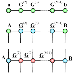
Refer to caption
Figure  25: Various forms of tensor train (TT) models: (Top) Scalar function can be expressed as x=𝒂T𝐆(2)𝐆(3)𝐆(M1)𝒃𝑥superscript𝒂𝑇superscript𝐆2superscript𝐆3superscript𝐆𝑀1𝒃x=\mbox{\boldmath$a$}^{T}{\bf G}^{(2)}{\bf G}^{(3)}\cdots{\bf G}^{(M-1)}\mbox{\boldmath$b$}, (middle) TT/MPS model of an M𝑀Mth-order data tensor (multidimensional vector) is expressed by 3rd-order tensors and two factor matrices as: 𝐗¯=𝐀,𝐆¯(2),𝐆¯(3),,𝐆¯(M1),𝐁¯𝐗𝐀superscript¯𝐆2superscript¯𝐆3superscript¯𝐆𝑀1𝐁\underline{{\bf X}}=\llbracket{\bf A},\underline{{\bf G}}^{(2)},\underline{{\bf G}}^{(3)},\ldots,\underline{{\bf G}}^{(M-1)},{\bf B}\rrbracket; (bottom) TT/MPO model of 2M2𝑀2Mth-order data tensor (multidimensional matrix) can be expressed by the chain of 3rd-order and 4th-order cores as: 𝐗¯=𝐀¯,𝐆¯(2),𝐆¯(3),,𝐆¯(M1),𝐁¯¯𝐗¯𝐀superscript¯𝐆2superscript¯𝐆3superscript¯𝐆𝑀1¯𝐁\underline{{\bf X}}=\llbracket\underline{{\bf A}},\underline{{\bf G}}^{(2)},\underline{{\bf G}}^{(3)},\ldots,\underline{{\bf G}}^{(M-1)},\underline{{\bf B}}\rrbracket.

(a)

Refer to caption

(b)

Refer to caption
Figure  26: Illustration of tensor train decomposition (TT/MPS) of a 4th-order data tensor 𝐗¯I1×I2×I3×I4¯𝐗superscriptsubscript𝐼1subscript𝐼2subscript𝐼3subscript𝐼4\underline{{\bf X}}\in\mathbb{R}^{I_{1}\times I_{2}\times I_{3}\times I_{4}}. (a) Tensor form via multilinear product of cores and/or the outer product of vectors (fibers) as sum of rank-1 tensors as: 𝐗¯𝐆¯(1)×31𝐆¯(2)×31𝐆¯(3)×31𝐆¯(4)=r1=1R1r2=1R2r3=1R3(𝒈 1,r1𝒈r1,r2(2)𝒈r2,r3(3)𝒈r3,1(4))¯𝐗subscriptsuperscript13subscriptsuperscript13subscriptsuperscript13superscript¯𝐆1superscript¯𝐆2superscript¯𝐆3superscript¯𝐆4superscriptsubscriptsubscript𝑟11subscript𝑅1superscriptsubscriptsubscript𝑟21subscript𝑅2superscriptsubscriptsubscript𝑟31subscript𝑅3subscript𝒈1subscript𝑟1subscriptsuperscript𝒈2subscript𝑟1subscript𝑟2subscriptsuperscript𝒈3subscript𝑟2subscript𝑟3subscriptsuperscript𝒈4subscript𝑟31\underline{{\bf X}}\cong\underline{{\bf G}}^{(1)}\times^{1}_{3}\underline{{\bf G}}^{(2)}\times^{1}_{3}\underline{{\bf G}}^{(3)}\times^{1}_{3}\underline{{\bf G}}^{(4)}=\sum_{r_{1}=1}^{R_{1}}\sum_{r_{2}=1}^{R_{2}}\sum_{r_{3}=1}^{R_{3}}(\mbox{\boldmath$g$}_{\,1,r_{1}}\;\circ\;\mbox{\boldmath$g$}^{(2)}_{\,r_{1},r_{2}}\;\circ\;\mbox{\boldmath$g$}^{(3)}_{\,r_{2},r_{3}}\;\circ\;\mbox{\boldmath$g$}^{(4)}_{\,r_{3},1}) (for R1=3,R2=4,R3=5;R0=R4=1formulae-sequencesubscript𝑅13formulae-sequencesubscript𝑅24formulae-sequencesubscript𝑅35subscript𝑅0subscript𝑅41R_{1}=3,R_{2}=4,R_{3}=5;R_{0}=R_{4}=1). All vectors (fibers) 𝒈rn1rn(n)Insubscriptsuperscript𝒈𝑛subscript𝑟𝑛1subscript𝑟𝑛superscriptsubscript𝐼𝑛\mbox{\boldmath$g$}^{(n)}_{r_{n-1}r_{n}}\in\mathbb{R}^{I_{n}} are considered as the column vectors. (b) Scalar form via slice matrices as: xi1,i2,i3,i4𝐆(1)(i1)𝐆(2)(i2)𝐆(3)(i3)𝐆(4)(i4)=r1,r2,r3,r4=1R1,R2,,RNg1,i1,r1(1)gr1,i2,r2(2)gr2,i3,r3(3)gr3,i4,1(4)subscript𝑥subscript𝑖1subscript𝑖2subscript𝑖3subscript𝑖4superscript𝐆1subscript𝑖1superscript𝐆2subscript𝑖2superscript𝐆3subscript𝑖3superscript𝐆4subscript𝑖4superscriptsubscriptsubscript𝑟1subscript𝑟2subscript𝑟3subscript𝑟41subscript𝑅1subscript𝑅2subscript𝑅𝑁subscriptsuperscript𝑔11subscript𝑖1subscript𝑟1subscriptsuperscript𝑔2subscript𝑟1subscript𝑖2subscript𝑟2subscriptsuperscript𝑔3subscript𝑟2subscript𝑖3subscript𝑟3subscriptsuperscript𝑔4subscript𝑟3subscript𝑖41x_{i_{1},i_{2},i_{3},i_{4}}\cong{\bf G}^{(1)}(i_{1})\;{\bf G}^{(2)}(i_{2})\;{\bf G}^{(3)}(i_{3})\;{\bf G}^{(4)}(i_{4})=\sum_{r_{1},r_{2},r_{3},r_{4}=1}^{R_{1},R_{2},\ldots,R_{N}}\;g^{(1)}_{1,i_{1},r_{1}}\;g^{(2)}_{r_{1},i_{2},r_{2}}\;g^{(3)}_{r_{2},i_{3},r_{3}}\;g^{(4)}_{r_{3},i_{4},1}.

The basic Tensor Train [21, 59, 60], called also Matrix Product State (MPS), in quantum physics [61, 62, 63, 64] decomposes the higher-order tensor into set of 3rd-order core tensors and factor matrices as illustrated in Figs. 2627. Note that the TT model is equivalent to the MPS only if the MPS has the open boundary conditions (OBC) [65, 66].
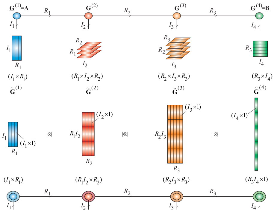
Refer to caption
Figure  27: Alternative representation of the tensor train decomposition (TT/MPS) expressed via strong Kronecker products of block matrices in the form of a vector as: 𝒙i1,i2,i3,i4¯𝐆~(1)||𝐆~(2)||𝐆~(3)||𝐆~(4)I1I2I3I4\mbox{\boldmath$x$}_{\overline{i_{1},i_{2},i_{3},i_{4}}}\cong\widetilde{\bf G}^{(1)}|\otimes|\;\widetilde{\bf G}^{(2)}\;|\otimes|\;\widetilde{\bf G}^{(3)}\;|\otimes|\;\widetilde{\bf G}^{(4)}\in\mathbb{R}^{I_{1}I_{2}I_{3}I_{4}}, where block matrices are defined as 𝐆~(n)Rn1In×Rnsuperscript~𝐆𝑛superscriptsubscript𝑅𝑛1subscript𝐼𝑛subscript𝑅𝑛\widetilde{\bf G}^{(n)}\in\mathbb{R}^{R_{n-1}I_{n}\times R_{n}}, with block vectors 𝒈rn1,rn(n)In×1subscriptsuperscript𝒈𝑛subscript𝑟𝑛1subscript𝑟𝑛superscriptsubscript𝐼𝑛1\mbox{\boldmath$g$}^{(n)}_{r_{n-1},r_{n}}\in\mathbb{R}^{I_{n}\times 1} for n=1,2,3,4𝑛1234n=1,2,3,4 and R0=R4=1subscript𝑅0subscript𝑅41R_{0}=R_{4}=1. For an illustrative purpose, we assumed that N=4𝑁4N=4, R1=3,R2=4formulae-sequencesubscript𝑅13subscript𝑅24R_{1}=3,R_{2}=4 and R3=5subscript𝑅35R_{3}=5.

The tensor train (TT/MPS) for an N𝑁Nth-order data tensor 𝐗¯I1,×I2,××IN¯𝐗superscriptsubscript𝐼1absentsubscript𝐼2absentsubscript𝐼𝑁\underline{{\bf X}}\in\mathbb{R}^{I_{1},\times I_{2},\times\cdots\times I_{N}} can be described in the various equivalent mathematical forms as follows.

  • In a compact tensor form using multilinear products:

    𝐗¯¯𝐗\displaystyle\underline{{\bf X}} \displaystyle\cong 𝐀×21𝐆¯(2)×31𝐆¯(3)×31×31𝐆¯(N1)×31𝐁superscriptsubscript31superscriptsubscript31superscriptsubscript31superscriptsubscript31superscriptsubscript21𝐀superscript¯𝐆2superscript¯𝐆3superscript¯𝐆𝑁1𝐁\displaystyle{\bf A}\times_{2}^{1}\underline{{\bf G}}^{(2)}\times_{3}^{1}\underline{{\bf G}}^{(3)}\times_{3}^{1}\cdots\times_{3}^{1}\underline{{\bf G}}^{(N-1)}\times_{3}^{1}{\bf B} (29)
    =\displaystyle= 𝐀,𝐆¯(2),𝐆¯(3),,𝐆¯(N1),𝐁,𝐀superscript¯𝐆2superscript¯𝐆3superscript¯𝐆𝑁1𝐁\displaystyle\llbracket{\bf A},\underline{{\bf G}}^{(2)},\underline{{\bf G}}^{(3)},\ldots,\underline{{\bf G}}^{(N-1)},{\bf B}\rrbracket,

    where 3rd-order cores are defined as 𝐆¯(n)Rn1×In×Rnsuperscript¯𝐆𝑛superscriptsubscript𝑅𝑛1subscript𝐼𝑛subscript𝑅𝑛\underline{{\bf G}}^{(n)}\in\mathbb{R}^{R_{n-1}\times I_{n}\times R_{n}} for n=2,3,,N1𝑛23𝑁1n=2,3,\ldots,N-1 (see Fig. 26 (a)).

  • By unfolding of cores 𝐆¯(n)superscript¯𝐆𝑛\underline{{\bf G}}^{(n)} and suitable reshaping of matrices, we can obtain other very useful mathematical and graphical descriptions of the MPS, for example, as summation of rank-1 tensors using outer (tensor) product (similar to CPD, Tucker and PARATREE formats):

    𝐗¯¯𝐗\displaystyle\underline{{\bf X}} \displaystyle\cong r1,r2,,rN1=1R1,R2,,RN1𝒈 1,r1(1)𝒈r1,r2(2)𝒈r2,r3(3)𝒈rN1,1(N)superscriptsubscriptsubscript𝑟1subscript𝑟2subscript𝑟𝑁11subscript𝑅1subscript𝑅2subscript𝑅𝑁1subscriptsuperscript𝒈11subscript𝑟1subscriptsuperscript𝒈2subscript𝑟1subscript𝑟2subscriptsuperscript𝒈3subscript𝑟2subscript𝑟3subscriptsuperscript𝒈𝑁subscript𝑟𝑁11\displaystyle\sum_{r_{1},r_{2},\ldots,r_{N-1}=1}^{R_{1},R_{2},\ldots,R_{N-1}}\mbox{\boldmath$g$}^{(1)}_{\,1,r_{1}}\;\circ\;\mbox{\boldmath$g$}^{(2)}_{r_{1},r_{2}}\;\circ\;\mbox{\boldmath$g$}^{(3)}_{r_{2},r_{3}}\;\circ\cdots\circ\;\mbox{\boldmath$g$}^{(N)}_{\,r_{N-1},1}

    where 𝒈rn1,rn(n)Insubscriptsuperscript𝒈𝑛subscript𝑟𝑛1subscript𝑟𝑛superscriptsubscript𝐼𝑛\mbox{\boldmath$g$}^{(n)}_{r_{n-1},r_{n}}\in\mathbb{R}^{I_{n}} are column vectors of matrices 𝐆(2)(n)=[𝒈1,1(n),𝒈2,1(n),,𝒈Rn1,1(n),𝒈1,2(n),,𝒈Rn1,Rn(n)]In×Rn1Rnsubscriptsuperscript𝐆𝑛2subscriptsuperscript𝒈𝑛11subscriptsuperscript𝒈𝑛21subscriptsuperscript𝒈𝑛subscript𝑅𝑛11subscriptsuperscript𝒈𝑛12subscriptsuperscript𝒈𝑛subscript𝑅𝑛1subscript𝑅𝑛superscriptsubscript𝐼𝑛subscript𝑅𝑛1subscript𝑅𝑛{\bf G}^{(n)}_{(2)}=[\mbox{\boldmath$g$}^{(n)}_{1,1},\;\mbox{\boldmath$g$}^{(n)}_{2,1},\ldots,\mbox{\boldmath$g$}^{(n)}_{R_{n-1},1},\mbox{\boldmath$g$}^{(n)}_{1,2},\ldots,\mbox{\boldmath$g$}^{(n)}_{R_{n-1},R_{n}}]\in\mathbb{R}^{I_{n}\times R_{n-1}R_{n}} (n=1,2,,N𝑛12𝑁n=1,2,\ldots,N), with R0=RN=1subscript𝑅0subscript𝑅𝑁1R_{0}=R_{N}=1. Note that 𝒈 1,r1(1)=𝒂r1subscriptsuperscript𝒈11subscript𝑟1subscript𝒂subscript𝑟1\mbox{\boldmath$g$}^{(1)}_{\,1,r_{1}}=\mbox{\boldmath$a$}_{r_{1}} are columns of the matrix 𝐀=[𝒂1,𝒂2,,𝒂R1]I1×R1𝐀subscript𝒂1subscript𝒂2subscript𝒂subscript𝑅1superscriptsubscript𝐼1subscript𝑅1{\bf A}=[\mbox{\boldmath$a$}_{1},\mbox{\boldmath$a$}_{2},\ldots,\mbox{\boldmath$a$}_{R_{1}}]\in\mathbb{R}^{I_{1}\times R_{1}}, while 𝒈rN1,1(N)=𝒃rN1subscriptsuperscript𝒈𝑁subscript𝑟𝑁11subscript𝒃subscript𝑟𝑁1\mbox{\boldmath$g$}^{(N)}_{r_{N-1},1}=\mbox{\boldmath$b$}_{r_{N-1}} are vector of the transposed factor matrix 𝐁T=[𝒃1,𝒃2,,𝒃RN1]IN×RN1superscript𝐁𝑇subscript𝒃1subscript𝒃2subscript𝒃subscript𝑅𝑁1superscriptsubscript𝐼𝑁subscript𝑅𝑁1{\bf B}^{T}=[\mbox{\boldmath$b$}_{1},\mbox{\boldmath$b$}_{2},\ldots,\mbox{\boldmath$b$}_{R_{N-1}}]\in\mathbb{R}^{I_{N}\times R_{N-1}} (see Fig. 26 (a)).

    The minimal (N1)𝑁1(N-1) tuple {R1,R2,,RN1}subscript𝑅1subscript𝑅2subscript𝑅𝑁1\{R_{1},R_{2},\ldots,R_{N-1}\} is called TT-rank (strictly speaking for the exact TT decomposition).

  • Alternatively, we can use the standard scalar form:

    xi1,i2,,iNsubscript𝑥subscript𝑖1subscript𝑖2subscript𝑖𝑁\displaystyle x_{i_{1},i_{2},\ldots,i_{N}} \displaystyle\cong r1,r2,,rN1=1R1,R2,,RN1g 1,i1,r1(1)gr1,i2,r2(2)grN1,iN,1(n),superscriptsubscriptsubscript𝑟1subscript𝑟2subscript𝑟𝑁11subscript𝑅1subscript𝑅2subscript𝑅𝑁1subscriptsuperscript𝑔11subscript𝑖1subscript𝑟1subscriptsuperscript𝑔2subscript𝑟1subscript𝑖2subscript𝑟2subscriptsuperscript𝑔𝑛subscript𝑟𝑁1subscript𝑖𝑁1\displaystyle\sum_{r_{1},r_{2},\ldots,r_{N-1}=1}^{R_{1},R_{2},\ldots,R_{N-1}}g^{(1)}_{\,1,i_{1},r_{1}}\;g^{(2)}_{r_{1},i_{2},r_{2}}\cdots g^{(n)}_{\,r_{N-1},i_{N},1},

    or equivalently using slice representations (see Fig. 26):

    xi1,i2,,iNsubscript𝑥subscript𝑖1subscript𝑖2subscript𝑖𝑁\displaystyle x_{i_{1},i_{2},\ldots,i_{N}} \displaystyle\cong 𝐆(1)(i1)𝐆(2)(i2)𝐆(N)(iN)superscript𝐆1subscript𝑖1superscript𝐆2subscript𝑖2superscript𝐆𝑁subscript𝑖𝑁\displaystyle{\bf G}^{(1)}(i_{1})\;{\bf G}^{(2)}(i_{2})\cdots{\bf G}^{(N)}(i_{N})
    =\displaystyle= 𝒈(1)T(i1)𝐆(2)(i2)𝒈(N)(iN),superscript𝒈1𝑇subscript𝑖1superscript𝐆2subscript𝑖2superscript𝒈𝑁subscript𝑖𝑁\displaystyle\mbox{\boldmath$g$}^{(1)\;T}(i_{1})\;{\bf G}^{(2)}(i_{2})\cdots\mbox{\boldmath$g$}^{(N)}(i_{N}),

    where slice matrices 𝐆(n)(in)=𝐆(n)(:,in,:)superscript𝐆𝑛subscript𝑖𝑛superscript𝐆𝑛:subscript𝑖𝑛:{\bf G}^{(n)}(i_{n})={\bf G}^{(n)}(:,i_{n},:) =𝐆Rn1,Rn(n)(in)Rn1×Rnabsentsubscriptsuperscript𝐆𝑛subscript𝑅𝑛1subscript𝑅𝑛subscript𝑖𝑛superscriptsubscript𝑅𝑛1subscript𝑅𝑛={\bf G}^{(n)}_{R_{n-1},R_{n}}(i_{n})\in\mathbb{R}^{R_{n-1}\times R_{n}} (with 𝐆(1)(i1)=𝒈(1)T(i1)1×R1superscript𝐆1subscript𝑖1superscript𝒈1𝑇subscript𝑖1superscript1subscript𝑅1{\bf G}^{(1)}(i_{1})=\mbox{\boldmath$g$}^{(1)\;T}(i_{1})\in\mathbb{R}^{1\times R_{1}} and 𝐆(N)(iN)=𝒈(N)(iN)RN1×1superscript𝐆𝑁subscript𝑖𝑁superscript𝒈𝑁subscript𝑖𝑁superscriptsubscript𝑅𝑁11{\bf G}^{(N)}(i_{N})=\mbox{\boldmath$g$}^{(N)}(i_{N})\in\mathbb{R}^{R_{N-1}\times 1}) are lateral slices of the cores 𝐆¯(n)Rn1×In×Rnsuperscript¯𝐆𝑛superscriptsubscript𝑅𝑛1subscript𝐼𝑛subscript𝑅𝑛\underline{{\bf G}}^{(n)}\in\mathbb{R}^{R_{n-1}\times I_{n}\times R_{n}} for n=1,2,,N𝑛12𝑁n=1,2,\ldots,N with R0=RN=1subscript𝑅0subscript𝑅𝑁1R_{0}=R_{N}=1.

  • By representing the cores 𝐆¯(n)Rn1×In×Rnsuperscript¯𝐆𝑛superscriptsubscript𝑅𝑛1subscript𝐼𝑛subscript𝑅𝑛\underline{{\bf G}}^{(n)}\in\mathbb{R}^{R_{n-1}\times I_{n}\times R_{n}} by unfolding matrices 𝐆~(n)=(𝐆(3)(n))TRn1In×Rnsuperscript~𝐆𝑛superscriptsubscriptsuperscript𝐆𝑛3𝑇superscriptsubscript𝑅𝑛1subscript𝐼𝑛subscript𝑅𝑛\widetilde{\bf G}^{(n)}=({\bf G}^{(n)}_{(3)})^{T}\in\mathbb{R}^{R_{n-1}I_{n}\times R_{n}} for n=1,2,,N𝑛12𝑁n=1,2,\ldots,N with R0=RN=1subscript𝑅0subscript𝑅𝑁1R_{0}=R_{N}=1 and considering them as block matrices with blocks 𝒈rn1,rn(n)In×1subscriptsuperscript𝒈𝑛subscript𝑟𝑛1subscript𝑟𝑛superscriptsubscript𝐼𝑛1\mbox{\boldmath$g$}^{(n)}_{r_{n-1},r_{n}}\in\mathbb{R}^{I_{n}\times 1}, we can express the TT/MPS in the matrix form via strong Kronecker products [67, 68, 69] (see Fig. 27 (c) and Fig. 28):

    𝒙i1,i2,,iN¯𝐆~(1)||𝐆~(2)||||𝐆~(N),\mbox{\boldmath$x$}_{{\overline{i_{1},i_{2},\ldots,i_{N}}}}\cong\widetilde{\bf G}^{(1)}\;|\otimes|\;\widetilde{\bf G}^{(2)}\;|\otimes|\cdots|\otimes|\;\widetilde{\bf G}^{(N)},\\ (33)

    where the vector 𝒙i1,i2,,iN¯=𝒙(1:N)I1I2INsubscript𝒙¯subscript𝑖1subscript𝑖2subscript𝑖𝑁subscript𝒙:1𝑁superscriptsubscript𝐼1subscript𝐼2subscript𝐼𝑁\mbox{\boldmath$x$}_{\overline{i_{1},i_{2},\ldots,i_{N}}}=\mbox{\boldmath$x$}_{(1:N)}\in\mathbb{R}^{I_{1}I_{2}\cdots I_{N}} denotes vectorization of the tensor 𝐗¯¯𝐗\underline{{\bf X}} in lexicographical order of indices and |||\otimes| denotes strong Kronecker product.

The strong Kronecker product of two block matrices (e.g., unfolding cores):

𝐀=[𝐀1,1𝐀1,R2𝐀R1,1𝐀R1,R2]R1I1×R2J1𝐀matrixsubscript𝐀11subscript𝐀1subscript𝑅2subscript𝐀subscript𝑅11subscript𝐀subscript𝑅1subscript𝑅2superscriptsubscript𝑅1subscript𝐼1subscript𝑅2subscript𝐽1\displaystyle{\bf A}=\begin{bmatrix}{\bf A}_{1,1}&\cdots&{\bf A}_{1,R_{2}}\\ \vdots&\ddots&\vdots\\ {\bf A}_{R_{1},1}&\cdots&{\bf A}_{R_{1},R_{2}}\end{bmatrix}\in\mathbb{R}^{R_{1}I_{1}\times R_{2}J_{1}}

and

𝐁=[𝐁1,1𝐁1,R3𝐁R2,1𝐁R2,R3]R2I2×R3J2𝐁matrixsubscript𝐁11subscript𝐁1subscript𝑅3subscript𝐁subscript𝑅21subscript𝐁subscript𝑅2subscript𝑅3superscriptsubscript𝑅2subscript𝐼2subscript𝑅3subscript𝐽2\displaystyle{\bf B}=\begin{bmatrix}\ {\bf B}_{1,1}&\cdots&{\bf B}_{1,R_{3}}\\ \vdots&\ddots&\vdots\\ {\bf B}_{R_{2},1}&\cdots&{\bf B}_{R_{2},R_{3}}\end{bmatrix}\in\mathbb{R}^{R_{2}I_{2}\times R_{3}J_{2}}

is defined as a block matrix

𝐂=𝐀||𝐁R1I1I2×R3J1J2,\displaystyle{\bf C}={\bf A}\;|\otimes|\;{\bf B}\in\mathbb{R}^{R_{1}I_{1}I_{2}\times R_{3}J_{1}J_{2}}, (34)

with blocks 𝐂r1,r3=r2=1R2𝐀r1,r2𝐁r2,r3I1I2×J1J2subscript𝐂subscript𝑟1subscript𝑟3superscriptsubscriptsubscript𝑟21subscript𝑅2tensor-productsubscript𝐀subscript𝑟1subscript𝑟2subscript𝐁subscript𝑟2subscript𝑟3superscriptsubscript𝐼1subscript𝐼2subscript𝐽1subscript𝐽2{\bf C}_{r_{1},r_{3}}=\sum_{r_{2}=1}^{R_{2}}{\bf A}_{r_{1},r_{2}}\otimes{\bf B}_{r_{2},r_{3}}\in\mathbb{R}^{I_{1}I_{2}\times J_{1}J_{2}}, where 𝐀r1,r2I1×J1subscript𝐀subscript𝑟1subscript𝑟2superscriptsubscript𝐼1subscript𝐽1{\bf A}_{r_{1},r_{2}}\in\mathbb{R}^{I_{1}\times J_{1}} and 𝐁r2,r3I2×J2subscript𝐁subscript𝑟2subscript𝑟3superscriptsubscript𝐼2subscript𝐽2{\bf B}_{r_{2},r_{3}}\in\mathbb{R}^{I_{2}\times J_{2}} are block matrices of 𝐀𝐀{\bf A} and 𝐁𝐁{\bf B}, respectively (see also Fig. 28 for graphical illustration).
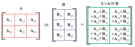
Refer to caption
Figure  28: Illustration of definition of the strong Kronecker product for two block matrices. The strong Kronecker product of two block matrices 𝐀=[𝐀r1,r2]R1I1×R2J1𝐀delimited-[]subscript𝐀subscript𝑟1subscript𝑟2superscriptsubscript𝑅1subscript𝐼1subscript𝑅2subscript𝐽1{\bf A}=[{\bf A}_{r_{1},r_{2}}]\in\mathbb{R}^{R_{1}I_{1}\times R_{2}J_{1}} and 𝐁=[𝐁r2,r3]R2I2×R3J2𝐁delimited-[]subscript𝐁subscript𝑟2subscript𝑟3superscriptsubscript𝑅2subscript𝐼2subscript𝑅3subscript𝐽2{\bf B}=[{\bf B}_{r_{2},r_{3}}]\in\mathbb{R}^{R_{2}I_{2}\times R_{3}J_{2}} is defined as the block matrix 𝐂=𝐀||𝐁R1I1I2×R3J1J2{\bf C}={\bf A}|\otimes|{\bf B}\in\mathbb{R}^{R_{1}I_{1}I_{2}\times R_{3}J_{1}J_{2}}, with blocks 𝐂r1,r3=r2=1R2𝐀r1,r2𝐁r2,r3I1I2×J1J2subscript𝐂subscript𝑟1subscript𝑟3superscriptsubscriptsubscript𝑟21subscript𝑅2tensor-productsubscript𝐀subscript𝑟1subscript𝑟2subscript𝐁subscript𝑟2subscript𝑟3superscriptsubscript𝐼1subscript𝐼2subscript𝐽1subscript𝐽2{\bf C}_{r_{1},r_{3}}=\sum_{r_{2}=1}^{R_{2}}{\bf A}_{r_{1},r_{2}}\otimes{\bf B}_{r_{2},r_{3}}\in\mathbb{R}^{I_{1}I_{2}\times J_{1}J_{2}}, for r1=1,2;r2=1,2,3formulae-sequencesubscript𝑟112subscript𝑟2123r_{1}=1,2;\;\;r_{2}=1,2,3 and r3=1,2subscript𝑟312r_{3}=1,2.

The matrix strong Kronecker product can be generalized to block tensors as follows: Let 𝐀¯=[𝐀¯r1,r2]R1I1×R2J1×K1¯𝐀matrixsubscript¯𝐀subscript𝑟1subscript𝑟2superscriptsubscript𝑅1subscript𝐼1subscript𝑅2subscript𝐽1subscript𝐾1\underline{{\bf A}}=\begin{bmatrix}\underline{{\bf A}}_{r_{1},r_{2}}\end{bmatrix}\in\mathbb{R}^{R_{1}I_{1}\times R_{2}J_{1}\times K_{1}} and 𝐁¯=[𝐁¯r2,r3]R2I2×R3J2×K2¯𝐁matrixsubscript¯𝐁subscript𝑟2subscript𝑟3superscriptsubscript𝑅2subscript𝐼2subscript𝑅3subscript𝐽2subscript𝐾2\underline{{\bf B}}=\begin{bmatrix}\underline{{\bf B}}_{r_{2},r_{3}}\end{bmatrix}\in\mathbb{R}^{R_{2}I_{2}\times R_{3}J_{2}\times K_{2}} are R1×R2subscript𝑅1subscript𝑅2R_{1}\times R_{2} and R2×R3subscript𝑅2subscript𝑅3R_{2}\times R_{3} block tensors, where blocks 𝐀¯r1,r2I1×J1×K1subscript¯𝐀subscript𝑟1subscript𝑟2superscriptsubscript𝐼1subscript𝐽1subscript𝐾1\underline{{\bf A}}_{r_{1},r_{2}}\in\mathbb{R}^{I_{1}\times J_{1}\times K_{1}} and 𝐁¯r2,r3I2×J2×K2subscript¯𝐁subscript𝑟2subscript𝑟3superscriptsubscript𝐼2subscript𝐽2subscript𝐾2\underline{{\bf B}}_{r_{2},r_{3}}\in\mathbb{R}^{I_{2}\times J_{2}\times K_{2}} are 3rd order tensors, then the strong Kronecker product of 𝐀¯¯𝐀\underline{{\bf A}} and 𝐁¯¯𝐁\underline{{\bf B}} is defined by the R1×R3subscript𝑅1subscript𝑅3R_{1}\times R_{3} block tensor

𝐂¯=[𝐂¯r1,r3]=𝐀¯||𝐁¯R1I1I2×R3J1J2×K1K2,\displaystyle\underline{{\bf C}}=\begin{bmatrix}\underline{{\bf C}}_{r_{1},r_{3}}\end{bmatrix}=\underline{{\bf A}}\ |\otimes|\ \underline{{\bf B}}\in\mathbb{R}^{R_{1}I_{1}I_{2}\times R_{3}J_{1}J_{2}\times K_{1}K_{2}}, (35)

where

𝐂¯r1,r3=r2=1R2𝐀¯r1,r2𝐁¯r2,r3I1I2×J1J2×K1K2,subscript¯𝐂subscript𝑟1subscript𝑟3superscriptsubscriptsubscript𝑟21subscript𝑅2tensor-productsubscript¯𝐀subscript𝑟1subscript𝑟2subscript¯𝐁subscript𝑟2subscript𝑟3superscriptsubscript𝐼1subscript𝐼2subscript𝐽1subscript𝐽2subscript𝐾1subscript𝐾2\underline{{\bf C}}_{r_{1},r_{3}}=\sum_{r_{2}=1}^{R_{2}}\underline{{\bf A}}_{r_{1},r_{2}}\otimes\underline{{\bf B}}_{r_{2},r_{3}}\in\mathbb{R}^{I_{1}I_{2}\times J_{1}J_{2}\times K_{1}K_{2}},

for r1=1,2,,R1subscript𝑟112subscript𝑅1r_{1}=1,2,\ldots,R_{1} and r3=1,2,,R3subscript𝑟312subscript𝑅3r_{3}=1,2,\ldots,R_{3}.

Refer to caption
Figure  29: The matrix tensor train decomposition (TT/MPO) for an 8th-order data tensor or equivalently multidimensional matrix 𝐗I¯1×I¯2𝐗superscriptsubscript¯𝐼1subscript¯𝐼2{\bf X}\in\mathbb{R}^{\overline{I}_{1}\times\overline{I}_{2}}, with I¯1=I1I3I5I7subscript¯𝐼1subscript𝐼1subscript𝐼3subscript𝐼5subscript𝐼7\overline{I}_{1}=I_{1}I_{3}I_{5}I_{7} and I¯2=I2I4I6I8subscript¯𝐼2subscript𝐼2subscript𝐼4subscript𝐼6subscript𝐼8\overline{I}_{2}=I_{2}I_{4}I_{6}I_{8}, expressed by the chain of 4th-order cores as: 𝐗¯𝐆¯(1)×41𝐆¯(2)×41𝐆¯(3)×41𝐆¯(4)=𝐆¯(1),𝐆¯(2),𝐆¯(3),𝐆¯(4)¯𝐗superscriptsubscript41superscriptsubscript41superscriptsubscript41superscript¯𝐆1superscript¯𝐆2superscript¯𝐆3superscript¯𝐆4superscript¯𝐆1superscript¯𝐆2superscript¯𝐆3superscript¯𝐆4\underline{{\bf X}}\cong\underline{{\bf G}}^{(1)}\;\times_{4}^{1}\;\underline{{\bf G}}^{(2)}\;\times_{4}^{1}\;\underline{{\bf G}}^{(3)}\;\times_{4}^{1}\;\underline{{\bf G}}^{(4)}=\llbracket\underline{{\bf G}}^{(1)},\underline{{\bf G}}^{(2)},\underline{{\bf G}}^{(3)},\underline{{\bf G}}^{(4)}\rrbracket or in a scalar form as xi1,i2,,i8r1=1R1r2=1R2r3=1R3g 1,i1,r1,i2(1)gr1,i2,r2,i4(2)gr2,i5,r3,i6(3)gr3,i7,i8,1(4)subscript𝑥subscript𝑖1subscript𝑖2subscript𝑖8superscriptsubscriptsubscript𝑟11subscript𝑅1superscriptsubscriptsubscript𝑟21subscript𝑅2superscriptsubscriptsubscript𝑟31subscript𝑅3subscriptsuperscript𝑔11subscript𝑖1subscript𝑟1subscript𝑖2subscriptsuperscript𝑔2subscript𝑟1subscript𝑖2subscript𝑟2subscript𝑖4subscriptsuperscript𝑔3subscript𝑟2subscript𝑖5subscript𝑟3subscript𝑖6subscriptsuperscript𝑔4subscript𝑟3subscript𝑖7subscript𝑖81x_{i_{1},i_{2},\ldots,i_{8}}\cong\sum_{r_{1}=1}^{R_{1}}\sum_{r_{2}=1}^{R_{2}}\sum_{r_{3}=1}^{R_{3}}g^{(1)}_{\,1,i_{1},r_{1},i_{2}}\;g^{(2)}_{r_{1},i_{2},r_{2},i_{4}}\;g^{(3)}_{r_{2},i_{5},r_{3},i_{6}}\;g^{(4)}_{r_{3},i_{7},i_{8},1}. Alternatively, the TT/MPO decomposition can be expressed in a compact and elegant matrix form as strong Kronecker product of block matrices 𝐆~(n)=𝐆(rn1,i2n1¯;rn,i2n¯)(n)Rn1I2n1×RnI2nsuperscript~𝐆𝑛subscriptsuperscript𝐆𝑛¯subscript𝑟𝑛1subscript𝑖2𝑛1¯subscript𝑟𝑛subscript𝑖2𝑛superscriptsubscript𝑅𝑛1subscript𝐼2𝑛1subscript𝑅𝑛subscript𝐼2𝑛\widetilde{\bf G}^{(n)}={\bf G}^{(n)}_{(\overline{r_{n-1},\,i_{2n-1}};\;\overline{r_{n},\,i_{2n}})}\in\mathbb{R}^{R_{n-1}\,I_{2n-1}\times R_{n}\,I_{2n}} (with blocks 𝐆rn1,rn(n)I2n1×I2nsubscriptsuperscript𝐆𝑛subscript𝑟𝑛1subscript𝑟𝑛superscriptsubscript𝐼2𝑛1subscript𝐼2𝑛{\bf G}^{(n)}_{r_{n-1},r_{n}}\in\mathbb{R}^{I_{2n-1}\times I_{2n}}) as: 𝐗(i1,i3,i5,i7¯;i2,i4,i6,i8¯)𝐆~(1)||𝐆~(2)||𝐆~(3)||𝐆~(4)I¯1×I¯2{\bf X}_{(\overline{i_{1},i_{3},i_{5},i_{7}}\;;\;\overline{i_{2},i_{4},i_{6},i_{8}})}\cong\widetilde{\bf G}^{(1)}\;|\otimes|\;\widetilde{\bf G}^{(2)}\;|\otimes|\;\widetilde{\bf G}^{(3)}\;|\otimes|\;\widetilde{\bf G}^{(4)}\in\mathbb{R}^{\overline{I}_{1}\times\overline{I}_{2}}. For simplicity, we assumed that R1=3subscript𝑅13R_{1}=3, R2=4subscript𝑅24R_{2}=4 and R3=5subscript𝑅35R_{3}=5, n=1,2,3,4.

Another important TT model, called matrix TT or MPO (Matrix Product Operator with Open Boundary Conditions), consists of a chain (train) of 3rd-order and 4th-order cores, as illustrated in Fig. 29. Note that a 3rd-order tensor can be represented equivalently as a block (column or row) vector in which each element (block) is a matrix (lateral slice) of the tensor, while a 4th-order tensor can represented equivalently as a block matrix. The TT/MPO model for 2N2𝑁2Nth-order tensor 𝐗¯I1×I2×I2N¯𝐗superscriptsubscript𝐼1subscript𝐼2subscript𝐼2𝑁\underline{{\bf X}}\in\mathbb{R}^{I_{1}\times I_{2}\times\cdots I_{2N}} can be described mathematically in the following general forms (see also Table III).

  • A) In the tensor compact form using multilinear products

    𝐗¯¯𝐗\displaystyle\underline{{\bf X}} \displaystyle\cong 𝐆¯(1)×41𝐆¯(2)×41×41𝐆¯(N)superscriptsubscript41superscriptsubscript41superscriptsubscript41superscript¯𝐆1superscript¯𝐆2superscript¯𝐆𝑁\displaystyle\underline{{\bf G}}^{(1)}\;\times_{4}^{1}\;\underline{{\bf G}}^{(2)}\;\times_{4}^{1}\;\cdots\times_{4}^{1}\;\underline{{\bf G}}^{(N)} (36)
    =\displaystyle= 𝐆¯(1),𝐆¯(2),,𝐆¯(N),superscript¯𝐆1superscript¯𝐆2superscript¯𝐆𝑁\displaystyle\llbracket\underline{{\bf G}}^{(1)},\underline{{\bf G}}^{(2)},\dots,\underline{{\bf G}}^{(N)}\rrbracket,

    where the cores are defined as 𝐆¯(n)Rn1×I2n1×I2n×Rnsuperscript¯𝐆𝑛superscriptsubscript𝑅𝑛1subscript𝐼2𝑛1subscript𝐼2𝑛subscript𝑅𝑛\underline{{\bf G}}^{(n)}\in\mathbb{R}^{R_{n-1}\times I_{2n-1}\times I_{2n}\times R_{n}}, with R0=RN=1subscript𝑅0subscript𝑅𝑁1R_{0}=R_{N}=1, (n=1,2,,N𝑛12𝑁n=1,2,\ldots,N).

  • B) Using the standard (rather long and tedious) scalar form:

    xi1,i2,,i2Nsubscript𝑥subscript𝑖1subscript𝑖2subscript𝑖2𝑁\displaystyle x_{i_{1},i_{2},\ldots,i_{2N}} \displaystyle\cong r1=1R1r2=1R2rN1=1RN1g1,i1,i2,r1(1)gr1,i3,i4,r2(2)superscriptsubscriptsubscript𝑟11subscript𝑅1superscriptsubscriptsubscript𝑟21subscript𝑅2superscriptsubscriptsubscript𝑟𝑁11subscript𝑅𝑁1subscriptsuperscript𝑔11subscript𝑖1subscript𝑖2subscript𝑟1subscriptsuperscript𝑔2subscript𝑟1subscript𝑖3subscript𝑖4subscript𝑟2\displaystyle\sum_{r_{1}=1}^{R_{1}}\sum_{r_{2}=1}^{R_{2}}\cdots\sum_{r_{N-1}=1}^{R_{N-1}}g^{(1)}_{1,i_{1},i_{2},r_{1}}\;g^{(2)}_{r_{1},i_{3},i_{4},r_{2}}\cdots
    \displaystyle\cdots grN2,i2N3,i2N2,rN1(N1)grN1,i2N1,i2N,1(N).subscriptsuperscript𝑔𝑁1subscript𝑟𝑁2subscript𝑖2𝑁3subscript𝑖2𝑁2subscript𝑟𝑁1subscriptsuperscript𝑔𝑁subscript𝑟𝑁1subscript𝑖2𝑁1subscript𝑖2𝑁1\displaystyle g^{(N-1)}_{r_{N-2},i_{2N-3},i_{2N-2},r_{N-1}}\;g^{(N)}_{r_{N-1},i_{2N-1},i_{2N},1}.
  • C) By matrix representations of cores, the TT/MPO decomposition can be expressed by strong Kronecker products (see Fig. 29):

    𝐗(i1,i3,,i2N1¯;i2,i4,,i2N¯)𝐆~(1)||𝐆~(2)||||𝐆~(N),{\bf X}_{(\overline{i_{1},i_{3},\ldots,i_{2N-1}}\;;\;\overline{i_{2},i_{4},\ldots,i_{2N}})}\cong\widetilde{\bf G}^{(1)}\;|\otimes|\;\widetilde{\bf G}^{(2)}\;|\otimes|\cdots\;|\otimes|\;\widetilde{\bf G}^{(N)},\\ (38)

    where 𝐗(i1,i3,,i2N1¯;i2,i4,,i2N¯)I1I3I2N1×I2I4I2Nsubscript𝐗¯subscript𝑖1subscript𝑖3subscript𝑖2𝑁1¯subscript𝑖2subscript𝑖4subscript𝑖2𝑁superscriptsubscript𝐼1subscript𝐼3subscript𝐼2𝑁1subscript𝐼2subscript𝐼4subscript𝐼2𝑁{\bf X}_{(\overline{i_{1},i_{3},\ldots,i_{2N-1}}\;;\;\overline{i_{2},i_{4},\ldots,i_{2N}})}\in\mathbb{R}^{I_{1}I_{3}\cdots I_{2N-1}\times I_{2}I_{4}\cdots I_{2N}} is unfolding matrix of 𝐗¯¯𝐗\underline{{\bf X}} in lexicographical order of indices and 𝐆~(n)Rn1I2n1×RnI2nsuperscript~𝐆𝑛superscriptsubscript𝑅𝑛1subscript𝐼2𝑛1subscript𝑅𝑛subscript𝐼2𝑛\widetilde{\bf G}^{(n)}\in\mathbb{R}^{R_{n-1}I_{2n-1}\times R_{n}I_{2n}} are block matrices with blocks 𝐆rn1,rn(n)I2n1×I2nsubscriptsuperscript𝐆𝑛subscript𝑟𝑛1subscript𝑟𝑛superscriptsubscript𝐼2𝑛1subscript𝐼2𝑛{\bf G}^{(n)}_{r_{n-1},r_{n}}\in\mathbb{R}^{I_{2n-1}\times I_{2n}} and the number of blocks Rn1×Rnsubscript𝑅𝑛1subscript𝑅𝑛R_{n-1}\times R_{n}. In the special case when ranks of the TT/MPO Rn=1,nsubscript𝑅𝑛1for-all𝑛R_{n}=1,\;\forall n the strong Kronecker products simplify to the standard Kronecker products.

TABLE III: Different forms of the Tensor Trains (TT): MPS and MPO (with OBC) representations of an N𝑁Nth-order tensor 𝐗¯I1×I1××IN¯𝐗superscriptsubscript𝐼1subscript𝐼1subscript𝐼𝑁\underline{{\bf X}}\in\mathbb{R}^{I_{1}\times I_{1}\times\cdots\times I_{N}} and a 2N2𝑁2Nth-order tensor 𝐘¯I1×J1×I2×J2×IN×JN¯𝐘superscriptsubscript𝐼1subscript𝐽1subscript𝐼2subscript𝐽2subscript𝐼𝑁subscript𝐽𝑁\underline{{\bf Y}}\in\mathbb{R}^{I_{1}\times J_{1}\times I_{2}\times J_{2}\cdots\times I_{N}\times J_{N}}, respectively. It is assumed that the TT rank is {R1,R2,,RN1}subscript𝑅1subscript𝑅2subscript𝑅𝑁1\{R_{1},R_{2},\ldots,R_{N-1}\}, with R0=RN=1subscript𝑅0subscript𝑅𝑁1R_{0}=R_{N}=1 (r0=rN=1subscript𝑟0subscript𝑟𝑁1r_{0}=r_{N}=1).

                            TT/MPS                             TT/MPO Scalar (standard) Representations xi1,i2,,iN=r1,r2,,rN1=1R1,R2,,RN1g 1,i1,r1(1)gr1,i2,r2(2)gr2,i3,r3(3)grN1,iN,1(N)subscript𝑥subscript𝑖1subscript𝑖2subscript𝑖𝑁superscriptsubscriptsubscript𝑟1subscript𝑟2subscript𝑟𝑁11subscript𝑅1subscript𝑅2subscript𝑅𝑁1subscriptsuperscript𝑔11subscript𝑖1subscript𝑟1subscriptsuperscript𝑔2subscript𝑟1subscript𝑖2subscript𝑟2subscriptsuperscript𝑔3subscript𝑟2subscript𝑖3subscript𝑟3subscriptsuperscript𝑔𝑁subscript𝑟𝑁1subscript𝑖𝑁1x_{\;i_{1},i_{2},\ldots,i_{N}}=\displaystyle{\sum_{r_{1},r_{2},\ldots,r_{N-1}=1}^{R_{1},R_{2},\ldots,R_{N-1}}}\;\;g^{(1)}_{\;1,i_{1},r_{1}}\;g^{(2)}_{\;r_{1},i_{2},r_{2}}\;g^{(3)}_{\;r_{2},i_{3},r_{3}}\cdots g^{(N)}_{\;r_{N-1},i_{N},1} yi1,j1,i2,j2,,iN,jN=r1,r2,,rN1=1R1,R2,,RN1g 1,i1,j1,r1(1)gr1,i2,j2,r2(2)grN1,iN,jN,1(N)subscript𝑦subscript𝑖1subscript𝑗1subscript𝑖2subscript𝑗2subscript𝑖𝑁subscript𝑗𝑁superscriptsubscriptsubscript𝑟1subscript𝑟2subscript𝑟𝑁11subscript𝑅1subscript𝑅2subscript𝑅𝑁1subscriptsuperscript𝑔11subscript𝑖1subscript𝑗1subscript𝑟1subscriptsuperscript𝑔2subscript𝑟1subscript𝑖2subscript𝑗2subscript𝑟2subscriptsuperscript𝑔𝑁subscript𝑟𝑁1subscript𝑖𝑁subscript𝑗𝑁1y_{i_{1},j_{1},i_{2},j_{2},\ldots,i_{N},j_{N}}=\displaystyle{\sum_{r_{1},r_{2},\ldots,r_{N-1}=1}^{R_{1},R_{2},\ldots,R_{N-1}}}\;\;g^{(1)}_{\;1,i_{1},j_{1},r_{1}}\;g^{(2)}_{\;r_{1},i_{2},j_{2},r_{2}}\cdots g^{(N)}_{\;r_{N-1},i_{N},j_{N},1} grn1,in,rn(n)subscriptsuperscript𝑔𝑛subscript𝑟𝑛1subscript𝑖𝑛subscript𝑟𝑛g^{(n)}_{\;r_{n-1},i_{n},r_{n}} entries of a 3rd-order core 𝐆¯(n)Rn1×In×Rnsuperscript¯𝐆𝑛superscriptsubscript𝑅𝑛1subscript𝐼𝑛subscript𝑅𝑛\underline{{\bf G}}^{(n)}\in\mathbb{R}^{R_{n-1}\times I_{n}\times R_{n}} grn1,in,jn,rn(n)subscriptsuperscript𝑔𝑛subscript𝑟𝑛1subscript𝑖𝑛subscript𝑗𝑛subscript𝑟𝑛g^{(n)}_{\;r_{n-1},i_{n},j_{n},r_{n}} entries of a 4th-order core 𝐆¯(n)Rn1×In×Jn×Rnsuperscript¯𝐆𝑛superscriptsubscript𝑅𝑛1subscript𝐼𝑛subscript𝐽𝑛subscript𝑅𝑛\underline{{\bf G}}^{(n)}\in\mathbb{R}^{R_{n-1}\times I_{n}\times J_{n}\times R_{n}} Slice Representations xi1,i2,,iN=𝐆(1)(i1)𝐆(2)(i2)𝐆(N1)(iN1)𝐆(N)(iN)subscript𝑥subscript𝑖1subscript𝑖2subscript𝑖𝑁superscript𝐆1subscript𝑖1superscript𝐆2subscript𝑖2superscript𝐆𝑁1subscript𝑖𝑁1superscript𝐆𝑁subscript𝑖𝑁x_{\;i_{1},i_{2},\ldots,i_{N}}={\bf G}^{(1)}(i_{1})\;{\bf G}^{(2)}(i_{2})\cdots{\bf G}^{(N-1)}(i_{N-1})\;{\bf G}^{(N)}(i_{N}) yi1,j1,i2,j2,,iN,jN=𝐆(1)(i1,j1)𝐆(2)(i2,j2)𝐆(N)(iN,jN)subscript𝑦subscript𝑖1subscript𝑗1subscript𝑖2subscript𝑗2subscript𝑖𝑁subscript𝑗𝑁superscript𝐆1subscript𝑖1subscript𝑗1superscript𝐆2subscript𝑖2subscript𝑗2superscript𝐆𝑁subscript𝑖𝑁subscript𝑗𝑁y_{i_{1},j_{1},i_{2},j_{2},\ldots,i_{N},j_{N}}={\bf G}^{(1)}(i_{1},j_{1})\;{\bf G}^{(2)}(i_{2},j_{2})\cdots{\bf G}^{(N)}(i_{N},j_{N}) 𝐆(n)(in)Rn1×Rnsuperscript𝐆𝑛subscript𝑖𝑛superscriptsubscript𝑅𝑛1subscript𝑅𝑛{\bf G}^{(n)}(i_{n})\in\mathbb{R}^{R_{n-1}\times R_{n}} lateral slices of cores 𝐆¯(n)superscript¯𝐆𝑛\underline{{\bf G}}^{(n)} 𝐆(n)(in,jn)Rn1×Rnsuperscript𝐆𝑛subscript𝑖𝑛subscript𝑗𝑛superscriptsubscript𝑅𝑛1subscript𝑅𝑛{\bf G}^{(n)}(i_{n},j_{n})\in\mathbb{R}^{R_{n-1}\times R_{n}} slices of cores 𝐆¯(n)superscript¯𝐆𝑛\underline{{\bf G}}^{(n)} Tensor Representations: Multilinear Products (tensor contractions) 𝐗¯=𝐆¯(1)×31𝐆¯(2)×31×31𝐆¯(N1)×31𝐆¯(N)¯𝐗superscriptsubscript31superscriptsubscript31superscriptsubscript31superscriptsubscript31superscript¯𝐆1superscript¯𝐆2superscript¯𝐆𝑁1superscript¯𝐆𝑁\underline{{\bf X}}=\underline{{\bf G}}^{(1)}\times_{3}^{1}\;\underline{{\bf G}}^{(2)}\times_{3}^{1}\;\cdots\times_{3}^{1}\;\underline{{\bf G}}^{(N-1)}\times_{3}^{1}\;\underline{{\bf G}}^{(N)}        𝐘¯=𝐆¯(1)×41𝐆¯(2)×41×41𝐆¯(N1)×41𝐆¯(N)¯𝐘superscriptsubscript41superscriptsubscript41superscriptsubscript41superscriptsubscript41superscript¯𝐆1superscript¯𝐆2superscript¯𝐆𝑁1superscript¯𝐆𝑁\underline{{\bf Y}}=\underline{{\bf G}}^{(1)}\times_{4}^{1}\;\underline{{\bf G}}^{(2)}\times_{4}^{1}\cdots\times_{4}^{1}\;\underline{{\bf G}}^{(N-1)}\times_{4}^{1}\;\underline{{\bf G}}^{(N)} 𝐆¯(n)Rn1×In×Rnsuperscript¯𝐆𝑛superscriptsubscript𝑅𝑛1subscript𝐼𝑛subscript𝑅𝑛\underline{{\bf G}}^{(n)}\in\mathbb{R}^{R_{n-1}\times I_{n}\times R_{n}}, (n=1,2,,N)𝑛12𝑁\;(n=1,2,\ldots,N)        𝐆¯(n)Rn1×In×Jn×Rnsuperscript¯𝐆𝑛superscriptsubscript𝑅𝑛1subscript𝐼𝑛subscript𝐽𝑛subscript𝑅𝑛\underline{{\bf G}}^{(n)}\in\mathbb{R}^{R_{n-1}\times I_{n}\times J_{n}\times R_{n}} Tensor Representations: Outer Products 𝐗¯=r1,r2,,rN1=1R1,R2,,RN1𝒈 1,r1(1)𝒈r1,r2(2)𝒈rN2,rN1(N1)𝒈rN1,1(N)¯𝐗superscriptsubscriptsubscript𝑟1subscript𝑟2subscript𝑟𝑁11subscript𝑅1subscript𝑅2subscript𝑅𝑁1subscriptsuperscript𝒈11subscript𝑟1subscriptsuperscript𝒈2subscript𝑟1subscript𝑟2subscriptsuperscript𝒈𝑁1subscript𝑟𝑁2subscript𝑟𝑁1subscriptsuperscript𝒈𝑁subscript𝑟𝑁11\underline{{\bf X}}=\displaystyle{\sum_{r_{1},r_{2},\ldots,r_{N-1}=1}^{R_{1},R_{2},\ldots,R_{N-1}}}\;\;\mbox{\boldmath$g$}^{(1)}_{\;1,r_{1}}\;\circ\;\mbox{\boldmath$g$}^{(2)}_{\;r_{1},r_{2}}\circ\cdots\circ\;\mbox{\boldmath$g$}^{(N-1)}_{\;r_{N-2},r_{N-1}}\;\circ\;\mbox{\boldmath$g$}^{(N)}_{\;r_{N-1},1} 𝐘¯=r1,r2,,rN1=1R1,R2,,RN1𝐆 1,r1(1)𝐆r1,r2(2)𝐆rN2,rN1(N1)𝐆rN1,1(N)¯𝐘superscriptsubscriptsubscript𝑟1subscript𝑟2subscript𝑟𝑁11subscript𝑅1subscript𝑅2subscript𝑅𝑁1subscriptsuperscript𝐆11subscript𝑟1subscriptsuperscript𝐆2subscript𝑟1subscript𝑟2subscriptsuperscript𝐆𝑁1subscript𝑟𝑁2subscript𝑟𝑁1subscriptsuperscript𝐆𝑁subscript𝑟𝑁11\underline{{\bf Y}}=\displaystyle{\sum_{r_{1},r_{2},\ldots,r_{N-1}=1}^{R_{1},R_{2},\ldots,R_{N-1}}}\;\;{\bf G}^{(1)}_{\;1,r_{1}}\;\circ\;{\bf G}^{(2)}_{\;r_{1},r_{2}}\circ\cdots\circ\;{\bf G}^{(N-1)}_{\;r_{N-2},r_{N-1}}\;\circ\;{\bf G}^{(N)}_{\;r_{N-1},1} 𝒈rn1,rn(n)Insubscriptsuperscript𝒈𝑛subscript𝑟𝑛1subscript𝑟𝑛superscriptsubscript𝐼𝑛\mbox{\boldmath$g$}^{(n)}_{\;r_{n-1},r_{n}}\in\mathbb{R}^{I_{n}} blocks of a matrix 𝐆~(n)=(𝐆(3)(n))TRn1In×Rnsuperscript~𝐆𝑛superscriptsubscriptsuperscript𝐆𝑛3𝑇superscriptsubscript𝑅𝑛1subscript𝐼𝑛subscript𝑅𝑛\widetilde{\bf G}^{(n)}=({\bf G}^{(n)}_{(3)})^{T}\in\mathbb{R}^{R_{n-1}I_{n}\times R_{n}} 𝐆rn1,rn(n)In×Jnsubscriptsuperscript𝐆𝑛subscript𝑟𝑛1subscript𝑟𝑛superscriptsubscript𝐼𝑛subscript𝐽𝑛{\bf G}^{(n)}_{\;r_{n-1},r_{n}}\in\mathbb{R}^{I_{n}\times J_{n}} blocks of a matrix 𝐆~(n)Rn1In×RnJnsuperscript~𝐆𝑛superscriptsubscript𝑅𝑛1subscript𝐼𝑛subscript𝑅𝑛subscript𝐽𝑛\widetilde{\bf G}^{(n)}\in\mathbb{R}^{R_{n-1}I_{n}\times R_{n}J_{n}} Vector/Matrix Representations: Kronecker and Strong Kronecker Products 𝒙(i1,,iN¯)=r1,r2,,rN1=1R1,R2,,RN1𝒈 1,r1(1)𝒈r1,r2(2)𝒈rN1,1(N)subscript𝒙¯subscript𝑖1subscript𝑖𝑁superscriptsubscriptsubscript𝑟1subscript𝑟2subscript𝑟𝑁11subscript𝑅1subscript𝑅2subscript𝑅𝑁1tensor-productsubscriptsuperscript𝒈11subscript𝑟1subscriptsuperscript𝒈2subscript𝑟1subscript𝑟2subscriptsuperscript𝒈𝑁subscript𝑟𝑁11\mbox{\boldmath$x$}_{(\overline{i_{1},\ldots,i_{N}})}=\displaystyle{\sum_{r_{1},r_{2},\ldots,r_{N-1}=1}^{R_{1},R_{2},\ldots,R_{N-1}}}\;\;\mbox{\boldmath$g$}^{(1)}_{\;1,r_{1}}\;\otimes\;\mbox{\boldmath$g$}^{(2)}_{\;r_{1},r_{2}}\otimes\cdots\otimes\;\mbox{\boldmath$g$}^{(N)}_{\;r_{N-1},1} 𝐘(i1,,iN¯);j1,,jN¯)=r1,r2,,rN1=1R1,R2,,RN1𝐆 1,r1(1)𝐆r1,r2(2)𝐆rN1,1(N){\bf Y}_{(\overline{i_{1},\ldots,i_{N}});\;\overline{j_{1},\ldots,j_{N}})}=\displaystyle{\sum_{r_{1},r_{2},\ldots,r_{N-1}=1}^{R_{1},R_{2},\ldots,R_{N-1}}}\;\;{\bf G}^{(1)}_{\;1,r_{1}}\;\otimes\;{\bf G}^{(2)}_{\;r_{1},r_{2}}\otimes\cdots\otimes\;{\bf G}^{(N)}_{\;r_{N-1},1} 𝒙(i1,,iN¯)=𝐆~(1)||𝐆~(2)||||𝐆~(N)I1I2IN\mbox{\boldmath$x$}_{(\overline{i_{1},\ldots,i_{N}})}=\widetilde{\bf G}^{(1)}\;|\otimes|\;\widetilde{\bf G}^{(2)}\;|\otimes|\cdots|\otimes|\;\widetilde{\bf G}^{(N)}\in\mathbb{R}^{I_{1}I_{2}\cdots I_{N}} 𝐘(i1,,iN¯);j1,,jN¯)=𝐆~(1)||𝐆~(2)||||𝐆~(N)I1IN×J1JN{\bf Y}_{(\overline{i_{1},\ldots,i_{N}});\;\overline{j_{1},\ldots,j_{N}})}=\widetilde{\bf G}^{(1)}\;|\otimes|\;\widetilde{\bf G}^{(2)}\;|\otimes|\cdots\;|\otimes|\;\widetilde{\bf G}^{(N)}\in\mathbb{R}^{I_{1}\cdots I_{N}\;\times\;J_{1}\cdots J_{N}} 𝐆~(n)Rn1In×Rnsuperscript~𝐆𝑛superscriptsubscript𝑅𝑛1subscript𝐼𝑛subscript𝑅𝑛\widetilde{\bf G}^{(n)}\in\mathbb{R}^{R_{n-1}I_{n}\times R_{n}} a block matrix with blocks 𝒈rn1,rn(n)Insubscriptsuperscript𝒈𝑛subscript𝑟𝑛1subscript𝑟𝑛superscriptsubscript𝐼𝑛\mbox{\boldmath$g$}^{(n)}_{r_{n-1},r_{n}}\in\mathbb{R}^{I_{n}}; 𝐆~(n)Rn1In×RnJnsuperscript~𝐆𝑛superscriptsubscript𝑅𝑛1subscript𝐼𝑛subscript𝑅𝑛subscript𝐽𝑛\widetilde{\bf G}^{(n)}\in\mathbb{R}^{R_{n-1}I_{n}\times R_{n}J_{n}} a block matrix with blocks 𝐆rn1,rn(n)In×Jnsubscriptsuperscript𝐆𝑛subscript𝑟𝑛1subscript𝑟𝑛superscriptsubscript𝐼𝑛subscript𝐽𝑛{\bf G}^{(n)}_{r_{n-1},r_{n}}\in\mathbb{R}^{I_{n}\times J_{n}}

The Tensor Train (TT) format [59], can be interpreted as a special case of the HT [7], where all nodes of the underlying tensor network are aligned and where, moreover, the leaf matrices are assumed to be identities (and thus need not be stored). An advantage of the TT format is its simpler practical implementation using SVD or alternative low-rank matrix approximations, as no binary tree need be involved [70, 21] (see Figs. 30 and 31).

Two different types of approaches to perform tensor approximation via TT exist [26]. The first class of methods is based on combining standard iterative algorithms, with a low-rank decompositions, such as SVD/QR or CUR or Cross-Approximations. Similar to the Tucker decomposition, the TT and HT decompositions are usually based on low rank approximation of generalized unfolding matrices 𝐗([n])subscript𝐗delimited-[]𝑛{\bf X}_{([n])}, and a good approximation in a decomposition for a given TT/HT-rank can be obtained using the truncated SVDs of the unfolding matrices [70, 59].
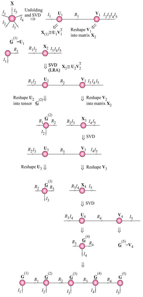
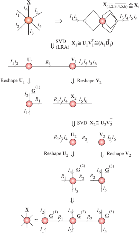
Refer to caption
Figure  30: Illustration of the SVD algorithm for TT/MPS for a 5th-order tensor. Instead of truncated SVD, we can employ any low-rank matrix factorizations, especially QR, CUR, SCA, ICA, NMF.
Refer to caption
Figure  31: SVD algorithm for TT/MPO for a 6th-order tensor. Instead of the SVD we can use alternative Low-Rank Approximations (constrained matrix factorizations, e.g., CUR or NMF).
Refer to caption
Figure  32: Extension of the ALS algorithm for TT decomposition. The idea is to optimize only one core tensor at a time (by a minimization of suitable cost function), while keeping the others fixed. Optimization of each core tensor is followed by an orthogonalization step via the QR or more expensive SVD decomposition. Factor matrices 𝐑𝐑{\bf R} are absorbed (incorporated) into the following core.
Refer to caption
Figure  33: Modified ALS (MALS) algorithm related to the Density Matrix Renormalization Group (DMRG) for TT decomposition. In each optimization step, two neighbor cores are merged. An optimization performed over merged “supercore”. After optimization in the next step we apply truncated SVD or other low-rank matrix factorizations (LRA) to separate the optimized supercore. For example, for nonnegative TT SVD steps can replaced by a non-negative matrix factorization (NMF) algorithm. Note that each optimization sub-problem is more expensive than the standard ALS and complexity increases but convergence speed may increase dramatically (see also [71, 72]).

In [55] Oseledets and Tyrtyshnikov proposed for TT decomposition a new approximative formula in which a N𝑁Nth-order data tensor is interpolated using special form of Cross-Approximation, which is a modification of CUR algorithm. The total number of entries and the complexity of the interpolation algorithm depend linearly on the order of data tensor N𝑁N, so the developed algorithm does not suffer from the curse of dimensionality. The TT-Cross-Approximation is analog to the SVD/HOSVD like algorithms for TT/MPS, but uses adaptive cross-approximation instead of the computationally more expensive SVD.

The second class of algorithms based on optimization of suitable designed cost functions, often with additional penalty or regularization terms. Optimization techniques include gradient descent, conjugate gradient, and Newton-like methods (see [71, 26] and references therein). Gradient descent methods leads often to the Alternating Least Squares (ALS) type of algorithms, which can be improved in various ways [71, 73] (see Fig. 32).

A quite successful improvement in TNs (TT, HT) is called the DMRG method. It joins two neighboring factors (cores), optimize the resulting “supernode”, and splits the result into separate factors by a low-rank matrix factorization [71, 72, 65, 66] (see Fig. 33).

Remark: In most optimization problems it is very convenient to present TT in a canonical form, in which all cores are left or right orthogonal [71, 74] (see also Fig. 32 and Fig. 33).

The N𝑁N-order core tensor is called right-orthogonal if

𝐆(1)𝐆(1)T=𝐈.subscript𝐆1subscriptsuperscript𝐆𝑇1𝐈\displaystyle{\bf G}_{(1)}{\bf G}^{T}_{(1)}={\bf I}. (39)

Analogously the N𝑁N-order core tensor is called left orthogonal if

𝐆(N)𝐆(N)T=𝐈.subscript𝐆𝑁subscriptsuperscript𝐆𝑇𝑁𝐈\displaystyle{\bf G}_{(N)}{\bf G}^{T}_{(N)}={\bf I}. (40)

In contrast, for the all-orthogonal core tensor we have 𝐆(n)𝐆(n)T=𝐈,nsubscript𝐆𝑛subscriptsuperscript𝐆𝑇𝑛𝐈for-all𝑛{\bf G}_{(n)}{\bf G}^{T}_{(n)}={\bf I},\;\;\forall n.

TT-Rounding TT–rounding (also called truncation or recompression) [55] is post-processing procedure to reduce the TT ranks which in the first stage after applying low-rank matrix factorizations are usually not optimal with respect of desired approximation errors. The optimal computation of TT-tensor is generally impossible without TT-rounding. The tensor expressed already in TT format is approximated by another TT-tensor with smaller TT-ranks but with prescribed accuracy of approximation ϵitalic-ϵ\epsilon. The most popular TT-rounding algorithm is based on the QR/SVD algorithm, which requires O(NIR3)𝑂𝑁𝐼superscript𝑅3O(NIR^{3}) operations [21, 75]. In practice, we avoid explicit construction of these matrices and the SVDs when truncating a tensor in TT decomposition to lower TT-rank. Such truncation algorithms for TT are described by Oseledets in [59]. In fact, the method exploits micro-iterations algorithm where the SVD is performed only on a relatively small core at each iteration. A similar approach has been developed by Grasedyck for the HT [76]. HT/TT algorithms that avoid the explicit computation of these SVDs when truncating a tensor that is already in tensor network format are discussed in [26, 72, 77].

TT Toolbox developed by Oseledets (http://spring.inm.ras.ru/osel/?page_id=24) is focussed on TT structures, and deals with the curse of dimensionality [75]. The Hierarchical Tucker (HT) toolbox by Kressner and Tobler (http://www.sam.math.ethz.ch/NLAgroup/htucker_toolbox.html) and Calculus library by Hackbusch, Waehnert and Espig, focuss mostly on HT and TT tensor networks [75, 25, 77]. See also recently developed TDALAB (http://bsp.brain.riken.jp/TDALAB and TENSORBOX http://www.bsp.brain.riken.jp/~phan that provide user-friendly interface and advanced algorithms for selected TD (Tucker, CPD) models [78, 79]. The <http://www.esat.kuleuven.be/sista/tensorlab/>Tensorlab toolbox builds upon the complex optimization framework and offers efficient numerical algorithms for computing the TDs with various constraints (e.g. nonnegativity, orthogonality) and the possibility to combine and jointly factorize dense, sparse and incomplete tensors [80]. The problems related to optimization of existing TN/TD algorithms are active area of research [26, 71, 73, 81, 82].

X Hierarchical Outer Product Tensor Approximation (HOPTA) and Kronecker Tensor Decompositions

Recent advances in TDs/TNs include, TT/HT [60, 71, 26], PARATREE [83], Block Term Decomposition (BTD) [84], Hierarchical Outer Product Tensor Approximation (HOPTA) and Kronecker Tensor Decomposition (KTD) [85, 86, 87].

HOPTA and KTD models can be expressed mathematically in simple nested (hierarchical) forms, respectively (see Fig. 34 and Fig. 35):

𝐗¯¯𝐗\displaystyle\underline{{\bf X}} \displaystyle\cong r=1R(𝐀¯r𝐁¯r),superscriptsubscript𝑟1𝑅subscript¯𝐀𝑟subscript¯𝐁𝑟\displaystyle\sum_{r=1}^{R}(\underline{{\bf A}}_{r}\circ\underline{{\bf B}}_{r}), (41)
𝐗¯~¯~𝐗\displaystyle\underline{\tilde{\bf X}} =\displaystyle= r=1R(𝐀¯r𝐁¯r),superscriptsubscript𝑟1𝑅tensor-productsubscript¯𝐀𝑟subscript¯𝐁𝑟\displaystyle\sum_{r=1}^{R}(\underline{{\bf A}}_{r}\otimes\underline{{\bf B}}_{r}), (42)

where each factor tensor can be represented recursively as 𝐀¯rr1=1R1(𝐀¯r1(1)𝐁¯r1(1))subscript¯𝐀𝑟superscriptsubscriptsubscript𝑟11subscript𝑅1subscriptsuperscript¯𝐀1subscript𝑟1subscriptsuperscript¯𝐁1subscript𝑟1\underline{{\bf A}}_{r}\cong\sum_{r_{1}=1}^{R_{1}}(\underline{{\bf A}}^{(1)}_{r_{1}}\circ\underline{{\bf B}}^{(1)}_{r_{1}}) or 𝐁¯rr2=1R2𝐀¯r2(2)𝐁¯r2(2)subscript¯𝐁𝑟superscriptsubscriptsubscript𝑟21subscript𝑅2subscriptsuperscript¯𝐀2subscript𝑟2subscriptsuperscript¯𝐁2subscript𝑟2\underline{{\bf B}}_{r}\cong\sum_{r_{2}=1}^{R_{2}}\underline{{\bf A}}^{(2)}_{r_{2}}\circ\underline{{\bf B}}^{(2)}_{r_{2}}, etc.

The Kronecker product of two tensors: 𝐀¯I1×I2××IN¯𝐀superscriptsubscript𝐼1subscript𝐼2subscript𝐼𝑁\underline{{\bf A}}\in\mathbb{R}^{I_{1}\times I_{2}\times\cdots\times I_{N}} and 𝐁¯J1×J2××JN¯𝐁superscriptsubscript𝐽1subscript𝐽2subscript𝐽𝑁\underline{{\bf B}}\in\mathbb{R}^{J_{1}\times J_{2}\times\cdots\times J_{N}} yields 𝐂¯=𝐀¯𝐁¯I1J2××INJN¯𝐂tensor-product¯𝐀¯𝐁superscriptsubscript𝐼1subscript𝐽2subscript𝐼𝑁subscript𝐽𝑁\underline{{\bf C}}=\underline{{\bf A}}\otimes\underline{{\bf B}}\in\mathbb{R}^{I_{1}J_{2}\times\cdots\times I_{N}J_{N}}, with entries ci1j1,,iNjN=ai1,,iNbj1,,jNsubscript𝑐tensor-productsubscript𝑖1subscript𝑗1tensor-productsubscript𝑖𝑁subscript𝑗𝑁subscript𝑎subscript𝑖1subscript𝑖𝑁subscript𝑏subscript𝑗1subscript𝑗𝑁c_{i_{1}\otimes j_{1},\ldots,i_{N}\otimes j_{N}}=a_{i_{1},\ldots,i_{N}}\>b_{j_{1},\ldots,j_{N}}, where the operator ¯¯tensor-product\bar{\otimes} for indices in=1,2,,Insubscript𝑖𝑛12subscript𝐼𝑛i_{n}=1,2,\ldots,I_{n} and jn=1,2,,Jnsubscript𝑗𝑛12subscript𝐽𝑛j_{n}=1,2,\ldots,J_{n} is defined as follows in,jn¯=jn+(in1)Jn¯subscript𝑖𝑛subscript𝑗𝑛subscript𝑗𝑛subscript𝑖𝑛1subscript𝐽𝑛\overline{i_{n},j_{n}}=j_{n}+(i_{n}-1)J_{n} (see Fig. 34).

Note that the 2N2𝑁2Nth-order sub-tensors 𝐀¯r𝐁¯rsubscript¯𝐀𝑟subscript¯𝐁𝑟\underline{{\bf A}}_{r}\circ\underline{{\bf B}}_{r} and 𝐀¯r𝐁¯rtensor-productsubscript¯𝐀𝑟subscript¯𝐁𝑟\underline{{\bf A}}_{r}\otimes\underline{{\bf B}}_{r} actually have the same elements, arranged differently. For example, if 𝐗¯=𝐀¯𝐁¯¯𝐗¯𝐀¯𝐁\underline{{\bf X}}=\underline{{\bf A}}\circ\underline{{\bf B}} and 𝐗¯=𝐀¯𝐁¯superscript¯𝐗tensor-product¯𝐀¯𝐁\underline{{\bf X}}^{\prime}=\underline{{\bf A}}\otimes\underline{{\bf B}}, where 𝐀¯J1×J2××JN¯𝐀superscriptsubscript𝐽1subscript𝐽2subscript𝐽𝑁\underline{{\bf A}}\in\mathbb{R}^{J_{1}\times J_{2}\times\cdots\times J_{N}} and 𝐁¯K1×K2××KN¯𝐁superscriptsubscript𝐾1subscript𝐾2subscript𝐾𝑁\underline{{\bf B}}\in\mathbb{R}^{K_{1}\times K_{2}\times\cdots\times K_{N}}, then xj1,j2,,jN,k1,k2,,kN=xk1+K1(j11),,kN(KN1)subscript𝑥subscript𝑗1subscript𝑗2subscript𝑗𝑁subscript𝑘1subscript𝑘2subscript𝑘𝑁subscriptsuperscript𝑥subscript𝑘1subscript𝐾1subscript𝑗11subscript𝑘𝑁subscript𝐾𝑁1x_{j_{1},j_{2},\ldots,j_{N},k_{1},k_{2},\ldots,k_{N}}=x^{\prime}_{k_{1}+K_{1}(j_{1}-1),\ldots,k_{N}(K_{N}-1)}.

Refer to caption
Figure  34: Kronecker product of two 4th-order tensors yields a tensor 𝐂¯=𝐀¯𝐁¯I1J1××I4J4¯𝐂tensor-product¯𝐀¯𝐁superscriptsubscript𝐼1subscript𝐽1subscript𝐼4subscript𝐽4\underline{{\bf C}}=\underline{{\bf A}}\otimes\underline{{\bf B}}\in\mathbb{R}^{I_{1}J_{1}\times\cdots\times I_{4}J_{4}}, with entries ck1,k2,,k4=ai1,,i4bj1,,j4subscript𝑐subscript𝑘1subscript𝑘2subscript𝑘4subscript𝑎subscript𝑖1subscript𝑖4subscript𝑏subscript𝑗1subscript𝑗4c_{k_{1},k_{2},\ldots,k_{4}}=a_{i_{1},\ldots,i_{4}}\>b_{j_{1},\ldots,j_{4}}, where kn=in,jn¯=in¯jn=jn+(in1)Jnsubscript𝑘𝑛¯subscript𝑖𝑛subscript𝑗𝑛subscript𝑖𝑛¯tensor-productsubscript𝑗𝑛subscript𝑗𝑛subscript𝑖𝑛1subscript𝐽𝑛k_{n}=\overline{i_{n},j_{n}}=i_{n}\bar{\otimes}j_{n}=j_{n}+(i_{n}-1)J_{n} (n=1,2,3,4𝑛1234n=1,2,3,4).
Refer to caption
Figure  35: Illustration of Hierarchical Outer Product Tensor Approximation (HOPTA) for higher-order data tensors of different orders. Each component tensor: 𝐀¯rsubscript¯𝐀𝑟\underline{{\bf A}}_{r}, 𝐁¯rsubscript¯𝐁𝑟\underline{{\bf B}}_{r} and/or 𝐂¯rsubscript¯𝐂𝑟\underline{{\bf C}}_{r} can be further decomposed using a suitable tensor network model. The model can be considered as an extension or generalization of the Block Term Decomposition (BTD) model to higher order tensors.
Refer to caption
Figure  36: Illustration of the decomposition of an 6th-order tensor using the BTD of rank-(Lr,Lr,1)subscript𝐿𝑟subscript𝐿𝑟1(L_{r},L_{r},1) as: 𝐗¯=r=1R𝐀¯r(𝒃r(1)𝒃r(2)𝒃r(3))¯𝐗superscriptsubscript𝑟1𝑅subscript¯𝐀𝑟superscriptsubscript𝒃𝑟1superscriptsubscript𝒃𝑟2superscriptsubscript𝒃𝑟3\underline{{\bf X}}=\sum_{r=1}^{R}\underline{{\bf A}}_{r}\circ(\mbox{\boldmath$b$}_{r}^{(1)}\circ\mbox{\boldmath$b$}_{r}^{(2)}\circ\mbox{\boldmath$b$}_{r}^{(3)}) [36], which can be considered as a special case of the HOPTA.

It is interesting to note that the KTD and HOPTA can be considered in special cases as a flexible form of Block Term Decomposition (BTD) introduced first by De Lathauwer [84, 88, 89, 36].

The definition of the tensor Kronecker product assumes that both core tensors 𝐀¯rsubscript¯𝐀𝑟\underline{{\bf A}}_{r} and 𝐁¯rsubscript¯𝐁𝑟\underline{{\bf B}}_{r} have the same order. It should be noted that vectors and matrices can be treated as tensors, e.g, matrix of dimension I×J𝐼𝐽I\times J can be treated formally as 3rd-order tensor of dimension I×J×1𝐼𝐽1I\times J\times 1. In fact, from the KTD model, we can generate many existing and emerging TDs by changing structures and orders of factor tensors: 𝐀¯rsubscript¯𝐀𝑟\underline{{\bf A}}_{r} and 𝐁¯rsubscript¯𝐁𝑟\underline{{\bf B}}_{r}, for example:

  • If 𝐀¯rsubscript¯𝐀𝑟\underline{{\bf A}}_{r} are rank-1 tensors of size I1×I2××INsubscript𝐼1subscript𝐼2subscript𝐼𝑁I_{1}\times I_{2}\times\cdots\times I_{N}, and 𝐁¯rsubscript¯𝐁𝑟\underline{{\bf B}}_{r} are scalars, rfor-all𝑟\forall r, then (42) expresses the rank-R𝑅R CPD.

  • If 𝐀¯rsubscript¯𝐀𝑟\underline{{\bf A}}_{r} are rank-Lrsubscript𝐿𝑟L_{r} tensors in the Kruskal (CP) format, of size I1×I2××IR×1××1subscript𝐼1subscript𝐼2subscript𝐼𝑅11I_{1}\times I_{2}\times\cdots\times I_{R}\times 1\times\cdots\times 1, and 𝐁¯rsubscript¯𝐁𝑟\underline{{\bf B}}_{r} are rank-1 CP tensor of size 1××1×IR+1××IN11subscript𝐼𝑅1subscript𝐼𝑁1\times\cdots\times 1\times I_{R+1}\times\cdots\times I_{N}, rfor-all𝑟\forall r, then (42) expresses the rank-(Lr1subscript𝐿𝑟1L_{r}\circ 1) BTD [84].

  • If 𝐀¯rsubscript¯𝐀𝑟\underline{{\bf A}}_{r} and 𝐁¯rsubscript¯𝐁𝑟\underline{{\bf B}}_{r} are expressed by KTDs, we have Nested Kronecker Tensor Decomposition (NKTD), where Tensor Train (TT) decomposition is a particular case [59, 90, 60]. In fact, the model (42) can be used for) the recursive TT-decompositions [59].

In this way, a large variety of tensor decomposition models can be generated. However, only some of them yield unique decompositions and to date only a few have found concrete applications is scientific computing.

The advantage of HOPTA models over BTD and KTD is that they are more flexible and can approximate very high order tensors with a relative small number of cores, and they allow us to model more complex data structures.

XI Tensorization and Quantization – Blessing of Dimensionality

XI-A Curse of Dimensionality

The term curse of dimensionality, in the context of tensors, refers to the fact that the number of elements of an N𝑁Nth-order (I×I××I)𝐼𝐼𝐼(I\times I\times\cdots\times I) tensor, INsuperscript𝐼𝑁I^{N}, grows exponentially with the tensor order N𝑁N. Tensors can easily become really big for very high order tensors since the size is exponentially growing with the number of dimensions ( ways , or modes ). For example, for the Tucker decomposition the number of entries of a original data tensor but also a core tensor scales exponentially in the tensor order, for instance, the number of entries of an N𝑁Nth-order (R×R××R)𝑅𝑅𝑅(R\times R\times\cdots\times R) core tensor is RNsuperscript𝑅𝑁R^{N}.

If all computations are performed on a CP tensor format and not on the raw data tensor itself, then instead of the original INsuperscript𝐼𝑁I^{N} raw data entries, the number of parameters in a CP representation reduces to NRI𝑁𝑅𝐼NRI, which scales linearly in N𝑁N and I𝐼I (see Table IV). This effectively bypasses the curse of dimensionality, however the CP approximation may involve numerical problems, since existing algorithms are not stable for high-order tensors. At the same time, existing algorithms for tensor networks, especially TT/HT ensure very good numerical properties (in contrast to CPD algorithms), making it possible to control an error of approximation i.e., to achieve a desired accuracy of approximation [60].

XI-B Quantized Tensor Networks

The curse of dimensionality can be overcome through quantized tensor networks, which represents a tensor of possibly very high-order as a set of sparsely interconnected low-order and very low dimensions cores [60, 91]. The concept of quantized tensor networks was first proposed by Khoromskij [92] and Oseledets [91]. The very low-dimensional cores are interconnected via tensor contractions to provide an efficient, highly compressed low-rank representation of a data tensor.

(a)
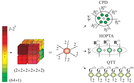
Refer to caption
(b)

Refer to caption

(c)

Refer to caption
Figure  37: Tensorization. (a) Illustration of the concept of tensorization of a (large-scale) vector (I=2K𝐼superscript2𝐾I=2^{K}) or matrix (2L×2Lsuperscript2𝐿superscript2𝐿2^{L}\times 2^{L}) into a higher-order tensor. In order to achieve super-compression through a suitable quantized tensor decomposition (e.g., decomposition into rank-1 tensors 𝐗¯r=1R𝒃r(1)𝒃r(2)𝒃r(6)¯𝐗superscriptsubscript𝑟1𝑅superscriptsubscript𝒃𝑟1superscriptsubscript𝒃𝑟2superscriptsubscript𝒃𝑟6\underline{{\bf X}}\cong\sum_{r=1}^{R}\mbox{\boldmath$b$}_{r}^{(1)}\circ\mbox{\boldmath$b$}_{r}^{(2)}\circ\cdots\circ\mbox{\boldmath$b$}_{r}^{(6)} or rank-q𝑞q terms using Hierarchical Outer Product Tensor Approximation (HOPTA) as: 𝐗¯r~=1R~𝐀r~𝐁r~𝐂r~¯𝐗superscriptsubscript~𝑟1~𝑅subscript𝐀~𝑟subscript𝐁~𝑟subscript𝐂~𝑟\underline{{\bf X}}\cong\sum_{\tilde{r}=1}^{\tilde{R}}{\bf A}_{\tilde{r}}\circ{\bf B}_{\tilde{r}}\circ{\bf C}_{\tilde{r}} or Quantized Tensor Train (QTT). (b) Symbolic representation of tensorization of the vector 𝒙I𝒙superscript𝐼\mbox{\boldmath$x$}\in\mathbb{R}^{I} into K𝐾Kth-order quantized tensor 𝐗¯2×2××2¯𝐗superscript222\underline{{\bf X}}\in\mathbb{R}^{2\times 2\times\cdots\times 2}. (c) Tensorization of a 3rd-order tensor 𝐗¯I1×I2×I3¯𝐗superscriptsubscript𝐼1subscript𝐼2subscript𝐼3\underline{{\bf X}}\in\mathbb{R}^{I_{1}\times I_{2}\times I_{3}} into (K1+K2+K3)subscript𝐾1subscript𝐾2subscript𝐾3(K_{1}+K_{2}+K_{3})th-order tensor 𝐘¯I1,1××I1,K1×I2,1××I3,K3¯𝐘superscriptsubscript𝐼11subscript𝐼1subscript𝐾1subscript𝐼21subscript𝐼3subscript𝐾3\underline{{\bf Y}}\in\mathbb{R}^{I_{1,1}\times\cdots\times I_{1,K_{1}}\times I_{2,1}\times\cdots\times I_{3,K_{3}}} with In,kn=qsubscript𝐼𝑛subscript𝑘𝑛𝑞I_{n,k_{n}}=q.

The procedure of creating a data tensor from lower-order original data is referred to as tensorization. In other words, lower-order data tensors can be reshaped (reformatted) into high-order tensors. The purpose of a such tensorization is to achieve super compression [92]. In general, very large-scale vectors or matrices can be easily tensorized to higher-order tensors, then efficiently compressed by applying a suitable TT decomposition; this is the underlying principle for big data analysis [91, 92]. For example, the quantization and tensorization of a huge vector 𝒙I𝒙superscript𝐼\mbox{\boldmath$x$}\in\mathbb{R}^{I}, I=2K𝐼superscript2𝐾I=2^{K} can be achieved through reshaping to give an (2×2××2)222(2\times 2\times\cdots\times 2) tensor 𝐗¯¯𝐗\underline{{\bf X}} of order K𝐾K, as illustrated in Figure 37 (a). Such a quantized tensor 𝐗¯¯𝐗\underline{{\bf X}} often admits low-rank approximations, so that a good compression of a huge vector 𝒙𝒙x can be achieved by enforcing a maximum possible low-rank structure on the tensor network.

Even more generally, an N𝑁Nth-order tensor 𝐗¯I1××IN¯𝐗superscriptsubscript𝐼1subscript𝐼𝑁\underline{{\bf X}}\in\mathbb{R}^{I_{1}\times\cdots\times I_{N}}, with In=qKnsubscript𝐼𝑛superscript𝑞subscript𝐾𝑛I_{n}=q^{K_{n}}, can be quantized in all modes simultaneously to yield a (q×q×q)𝑞𝑞𝑞(q\times q\times\cdots q) quantized tensor 𝐘¯¯𝐘\underline{{\bf Y}} of higher-order, with small q𝑞q, (see Fig. 37 (c) and Fig. 38).

In the example shown in Fig. 38 the Tensor Train of a huge 3rd-order tensor cab be represented by the strong Kronecker products of block tensors with relatively small 3rd-order blocks.

(a)
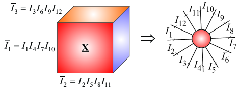
Refer to caption

(b)

Refer to caption
Figure  38: Example of tensorization and decomposition of a large-scale 3rd-order tensor 𝐗¯I¯1×I¯2×I¯3¯𝐗superscriptsubscript¯𝐼1subscript¯𝐼2subscript¯𝐼3\underline{{\bf X}}\in\mathbb{R}^{\overline{I}_{1}\times\overline{I}_{2}\times\overline{I}_{3}} into 12th-order tensor assuming that I¯1=I1I4I7I10subscript¯𝐼1subscript𝐼1subscript𝐼4subscript𝐼7subscript𝐼10\overline{I}_{1}=I_{1}I_{4}I_{7}I_{10}, I¯2=I2I5I8I11subscript¯𝐼2subscript𝐼2subscript𝐼5subscript𝐼8subscript𝐼11\overline{I}_{2}=I_{2}I_{5}I_{8}I_{11} and I¯3=I3I6I9I12subscript¯𝐼3subscript𝐼3subscript𝐼6subscript𝐼9subscript𝐼12\overline{I}_{3}=I_{3}I_{6}I_{9}I_{12}: (a) Tensorization and (b) representation of the higher-order tensor via generalized Tensor Train refereed to as the Tensor Product States (TPS). The data tensor can be expressed by strong Kronecker product of block tensors as 𝐗¯𝐆¯~(1)||𝐆¯~(2)||𝐆¯~(3)||𝐆¯~(4)I¯1×I¯2×I¯3\underline{{\bf X}}\cong\underline{\widetilde{\bf G}}^{(1)}\;|\otimes|\;\underline{\widetilde{\bf G}}^{(2)}\;|\otimes|\;\underline{\widetilde{\bf G}}^{(3)}\;|\otimes|\;\underline{\widetilde{\bf G}}^{(4)}\in\mathbb{R}^{\overline{I}_{1}\times\overline{I}_{2}\times\overline{I}_{3}}, where each block of the core 𝐆¯~(n)Rn1I3n2×RnI3n1×I3nsuperscript¯~𝐆𝑛superscriptsubscript𝑅𝑛1subscript𝐼3𝑛2subscript𝑅𝑛subscript𝐼3𝑛1subscript𝐼3𝑛\underline{\widetilde{\bf G}}^{(n)}\in\mathbb{R}^{R_{n-1}I_{3n-2}\times R_{n}I_{3n-1}\times I_{3n}} is a 3rd-order tensor of dimensions (I3n2×I3n1×I3n)subscript𝐼3𝑛2subscript𝐼3𝑛1subscript𝐼3𝑛(I_{3n-2}\times I_{3n-1}\times I_{3n}), with R0=R4=1subscript𝑅0subscript𝑅41R_{0}=R_{4}=1 for n=1,2,3,4𝑛1234n=1,2,3,4.

Recall that the strong Kronecker product of two block cores: 𝐆¯(n)=[𝐆¯1,1(n)𝐆¯1,Rn(n)𝐆¯Rn1,1(n)𝐆¯Rn1,Rn(n)]Rn1I3n2×RnI3n1×I3nsuperscript¯𝐆𝑛matrixsubscriptsuperscript¯𝐆𝑛11subscriptsuperscript¯𝐆𝑛1subscript𝑅𝑛subscriptsuperscript¯𝐆𝑛subscript𝑅𝑛11subscriptsuperscript¯𝐆𝑛subscript𝑅𝑛1subscript𝑅𝑛superscriptsubscript𝑅𝑛1subscript𝐼3𝑛2subscript𝑅𝑛subscript𝐼3𝑛1subscript𝐼3𝑛\underline{{\bf G}}^{(n)}=\begin{bmatrix}\underline{{\bf G}}^{(n)}_{1,1}&\cdots&\underline{{\bf G}}^{(n)}_{1,R_{n}}\\ \vdots&\ddots&\vdots\\ \underline{{\bf G}}^{(n)}_{R_{n-1},1}&\cdots&\underline{{\bf G}}^{(n)}_{R_{n-1},R_{n}}\end{bmatrix}\in\mathbb{R}^{R_{n-1}I_{3n-2}\times R_{n}I_{3n-1}\times I_{3n}} and

𝐆¯(n+1)=[𝐆¯1,1(n+1)𝐆¯1,Rn+1(n+1)𝐆¯Rn,1(n+1)𝐆¯Rn,Rn+1(n+1)]RnI3n+1×Rn+1I3n+2×I3n+3superscript¯𝐆𝑛1matrixsubscriptsuperscript¯𝐆𝑛111subscriptsuperscript¯𝐆𝑛11subscript𝑅𝑛1subscriptsuperscript¯𝐆𝑛1subscript𝑅𝑛1subscriptsuperscript¯𝐆𝑛1subscript𝑅𝑛subscript𝑅𝑛1superscriptsubscript𝑅𝑛subscript𝐼3𝑛1subscript𝑅𝑛1subscript𝐼3𝑛2subscript𝐼3𝑛3\underline{{\bf G}}^{(n+1)}=\begin{bmatrix}\underline{{\bf G}}^{(n+1)}_{1,1}&\cdots&\underline{{\bf G}}^{(n+1)}_{1,R_{n+1}}\\ \vdots&\ddots&\vdots\\ \underline{{\bf G}}^{(n+1)}_{R_{n},1}&\cdots&\underline{{\bf G}}^{(n+1)}_{R_{n},R_{n+1}}\end{bmatrix}\in\mathbb{R}^{R_{n}I_{3n+1}\times R_{n+1}I_{3n+2}\times I_{3n+3}} is defined as a block tensor

𝐂¯¯𝐂\displaystyle\underline{{\bf C}} =\displaystyle= 𝐆¯(n)||𝐆¯(n+1)\displaystyle\underline{{\bf G}}^{(n)}\;|\otimes|\;\underline{{\bf G}}^{(n+1)} (43)
Rn1I3n2I3n+1×Rn+1I3n1I3n+2×I3nI3n+3,absentsuperscriptsubscript𝑅𝑛1subscript𝐼3𝑛2subscript𝐼3𝑛1subscript𝑅𝑛1subscript𝐼3𝑛1subscript𝐼3𝑛2subscript𝐼3𝑛subscript𝐼3𝑛3\displaystyle\in\mathbb{R}^{R_{n-1}I_{3n-2}I_{3n+1}\times R_{n+1}I_{3n-1}I_{3n+2}\times I_{3n}I_{3n+3}},

with blocks 𝐆¯rn1,rn+1(n)=rn=1Rn𝐆¯rn1,rn(n)𝐆¯rn,rn+1(n+1)subscriptsuperscript¯𝐆𝑛subscript𝑟𝑛1subscript𝑟𝑛1superscriptsubscriptsubscript𝑟𝑛1subscript𝑅𝑛tensor-productsubscriptsuperscript¯𝐆𝑛subscript𝑟𝑛1subscript𝑟𝑛subscriptsuperscript¯𝐆𝑛1subscript𝑟𝑛subscript𝑟𝑛1\underline{{\bf G}}^{(n)}_{r_{n-1},r_{n+1}}=\sum_{r_{n}=1}^{R_{n}}\underline{{\bf G}}^{(n)}_{r_{n-1},r_{n}}\otimes\underline{{\bf G}}^{(n+1)}_{r_{n},r_{n+1}}, where 𝐆¯rn1,rn(n)I3n2×I3n1×I3nsubscriptsuperscript¯𝐆𝑛subscript𝑟𝑛1subscript𝑟𝑛superscriptsubscript𝐼3𝑛2subscript𝐼3𝑛1subscript𝐼3𝑛\underline{{\bf G}}^{(n)}_{r_{n-1},r_{n}}\in\mathbb{R}^{I_{3n-2}\times I_{3n-1}\times I_{3n}} and 𝐆¯rn,rn+1(n+1)I3n+1×I3n+2×I3n+3subscriptsuperscript¯𝐆𝑛1subscript𝑟𝑛subscript𝑟𝑛1superscriptsubscript𝐼3𝑛1subscript𝐼3𝑛2subscript𝐼3𝑛3\underline{{\bf G}}^{(n+1)}_{r_{n},r_{n+1}}\in\mathbb{R}^{I_{3n+1}\times I_{3n+2}\times I_{3n+3}} are block tensors of 𝐆¯(n)superscript¯𝐆𝑛\underline{{\bf G}}^{(n)} and 𝐆¯(n+1)superscript¯𝐆𝑛1\underline{{\bf G}}^{(n+1)}, respectively.

In practice, a fine (q=2,3,4𝑞234q=2,3,4 ) quantization is desirable to create as many virtual modes as possible, thus allowing us to implement efficient low-rank tensor approximations. For example, the binary encoding (q=2𝑞2q=2) reshapes an N𝑁Nth-order tensor with (2K1×2K2××2KN)superscript2subscript𝐾1superscript2subscript𝐾2superscript2subscript𝐾𝑁(2^{K_{1}}\times 2^{K_{2}}\times\cdots\times 2^{K_{N}}) elements into a tensor of order (K1+K2++KN)subscript𝐾1subscript𝐾2subscript𝐾𝑁(K_{1}+K_{2}+\cdots+K_{N}), with the same number of elements. In other words, the idea of the quantized tensor is quantization of each n𝑛n-th physical mode (dimension) by replacing it with Knsubscript𝐾𝑛K_{n} virtual modes, provided that the corresponding mode size Insubscript𝐼𝑛I_{n} are factorized as In=In,1In,2In,Knsubscript𝐼𝑛subscript𝐼𝑛1subscript𝐼𝑛2subscript𝐼𝑛subscript𝐾𝑛I_{n}=I_{n,1}I_{n,2}\cdots I_{n,K_{n}}. This corresponds to reshaping the n𝑛n-th mode of size Insubscript𝐼𝑛I_{n} into Knsubscript𝐾𝑛K_{n} modes of sizes In,1,In,2,,In,Knsubscript𝐼𝑛1subscript𝐼𝑛2subscript𝐼𝑛subscript𝐾𝑛I_{n,1},I_{n,2},\ldots,I_{n,K_{n}}.

The TT decomposition applied to quantized tensors is referred to as the QTT; it was first introduced as a compression scheme for large-scale matrices [91], and also independently for more general settings [92, 74, 93, 94, 69]. The attractive property of QTT is that not only its rank is typically small (below 10) but it is almost independent or at least uniformly bounded by data size (even for I=250𝐼superscript250I=2^{50}), providing a logarithmic (sub-linear) reduction of storage requirements: 𝒪(IN)𝒪(Nlogq(I))𝒪superscript𝐼𝑁𝒪𝑁subscript𝑞𝐼{\cal{O}}(I^{N})\rightarrow{\cal{O}}(N\log_{q}(I)) – so-called super-compression [92].

TABLE IV: Storage complexities of tensor decomposition models for an N𝑁Nth-order tensor 𝐗¯I1×I2××IN¯𝐗superscriptsubscript𝐼1subscript𝐼2subscript𝐼𝑁\underline{{\bf X}}\in\mathbb{R}^{I_{1}\times I_{2}\times\cdots\times I_{N}}, for which the original storage complexity is 𝒪(IN)𝒪superscript𝐼𝑁{\cal{O}}(I^{N}), where I=max{I1,I2,,IN}𝐼subscript𝐼1subscript𝐼2subscript𝐼𝑁I=\max\{I_{1},I_{2},\ldots,I_{N}\}, while R𝑅R is an upper bound on the ranks of tensor decompositions considered, that is R=max{R1,R2,,RN1}𝑅subscript𝑅1subscript𝑅2subscript𝑅𝑁1R=\max\{R_{1},R_{2},\ldots,R_{N-1}\} or R=max{R1,R2,,RN}𝑅subscript𝑅1subscript𝑅2subscript𝑅𝑁R=\max\{R_{1},R_{2},\ldots,R_{N}\}.

1. CPD 𝒪(NIR)𝒪𝑁𝐼𝑅{\cal{O}}(NIR) 2. Tucker 𝒪(NIR+RN)𝒪𝑁𝐼𝑅superscript𝑅𝑁{\cal{O}}(NIR+R^{N}) 3. TT/MPS 𝒪(NIR2)𝒪𝑁𝐼superscript𝑅2{\cal{O}}(NIR^{2}) 4. TT/MPO 𝒪(NI2R2)𝒪𝑁superscript𝐼2superscript𝑅2{\cal{O}}(NI^{2}R^{2}) 5. Quantized TT/MPS (QTT) 𝒪(NR2logq(I))𝒪𝑁superscript𝑅2subscript𝑞𝐼{\cal{O}}(NR^{2}\log_{q}(I)) 6. QTT+Tucker 𝒪(NR2logq(I)+NR3)𝒪𝑁superscript𝑅2subscript𝑞𝐼𝑁superscript𝑅3{\cal{O}}(NR^{2}\log_{q}(I)+NR^{3}) 7. Hierarchical Tucker (HT) 𝒪(NIR+NR3)𝒪𝑁𝐼𝑅𝑁superscript𝑅3{\cal{O}}(NIR+NR^{3})

Compared to the TT decomposition (without quantization), the QTT format often represents more deep structure in the data by introducing some “virtual” dimensions. The high compressibility of the QTT-approximation is a consequence of the noticeable separability properties in the quantized tensor for suitably structured data.

The fact that the TT/QTT ranks are often moderate or even low, e.g., constant or growing linearly with respect to N𝑁N and constant or growing logarithmically with respect to I𝐼I, is an important issue in the context of big data analytic and has been addressed so far mostly experimentally (see [60, 92, 26] and references therein). On the other hand, the high efficiency of multilinear algebra in the TT/QTT algorithms based on the well-posedness of the TT low-rank approximation problems and the fact that such problems are solved quite efficiently with the use of SVD/QR, CUR and other cross-approximation techniques.

In general, tensor networks can be considered as distributed high-dimensional tensors built up from many core tensors of low dimension through specific tensor contractions. Indeed, tensor networks (TT, MPS, MPO, PEPS and HT) have already been successfully used to solve intractable problems in computational quantum chemistry and in scientific computing [63, 95, 94, 69, 68, 96].

However, in some cases, the ranks of the TT or QTT formats grow quite significantly with the linearly increasing of approximation accuracy. To overcome this problem, new tensor models of tensor approximation were developed, e.g., Dolgov and Khoromskij, proposed the QTT-Tucker format [74] (see Fig. 39), which exploits the TT approximation not only for the Tucker core tensor, but also QTT for the factor matrices. This model allows distributed computing, often with bounded ranks and to avoid the curse of dimensionality. For very large scale tensors we can apply a more advanced approach in which factor matrices are tensorized to higher-order tensors and then represented by TTs as illustrated in Fig. 39.

(a)

Refer to caption

(b)
Refer to caption

Figure  39: QTT-Tucker format. (a) Distributed representation of a large matrix 𝐀nIn×Rnsubscript𝐀𝑛superscriptsubscript𝐼𝑛subscript𝑅𝑛{\bf A}_{n}\in\mathbb{R}^{I_{n}\times R_{n}} with large dimension of Insubscript𝐼𝑛I_{n} via QTT by tensorization of the matrix to high-order quantized tensor and next by performing QTT decomposition. (b) Distributed representation of a large-scale N𝑁Nth-order Tucker model via a quantized TT model in which core tensor and all large-scale factor matrices 𝐀nsubscript𝐀𝑛{\bf A}_{n} (n=1,2,,N𝑛12𝑁n=1,2,\ldots,N) are represented by tensor trains [74].

Modern methods of tensor approximations combine many TNs and TDs formats including the CPD, BTD, Tucker, TT, HT decompositions and HOPTA (see Fig. 35) low-parametric tensor format. The concept tensorization and by representation of a very high-order tensor in tensor network formats (TT/QTT, HT, QTT-Tucker) allows us to treat efficiently a very large-scale structured data that admit low rank tensor network approximations. TT/QTT/HT tensor networks have already found promising applications in very large-scale problems in scientific computing, such as eigenanalysis, super-fast Fourier transforms, and solving huge systems of large linear equations (see [93, 97, 74, 66, 26] and references therein).

In summary, the main concept or approach is to apply a suitable tensorization and quantization of tensor data and then perform approximative decomposition of this data into a tensor network and finally perform all computations (tensors/matrix/vectors operations, optimizations) in tensor network formats.

XII Conclusions and Future Directions

Tensor networks can be considered as a generalization and extension of TDs and are promising tools for the analysis of big data due to their extremely good compression abilities and distributed and parallel processing. TDs have already found application in generalized multivariate regression, multi-way blind source separation, sparse representation and coding, feature extraction, classification, clustering and data assimilation. Unique advantages of tensor networks include potential ability of tera- or even peta-byte scaling and distributed fault-tolerant computations.

Overall, the benefits of multiway (tensor) analysis methods can be summarized as follows:

  • “Super” compression of huge multidimensional, structured data which admits a low-rank approximation via TNs of high-order tensors by extracting factor matrices and/or core tensors of low-rank and low-order and perform all mathematical manipulations in tensor formats (especially, TT and HT formats).

  • A compact and very flexible approximate representation of structurally rich data by accounting for their spatio-temporal and spectral dependencies.

  • Opportunity to establish statistical links between cores, factors, components or hidden latent variables for blocks of data.

  • Possibility to operate with noisy, incomplete, missing data by using powerful low-rank tensor/matrix approximation techniques.

  • A framework to incorporate various diversities or constraints in different modes and thus naturally extend the standard (2-way) CA methods to large-scale multidimensional data.

Many challenging problems related to low-rank tensor approximations remain to be addressed.

  • A whole new area emerges when several TNs which operate on different datasets are coupled or linked.

  • As the complexity of big data increases, this requires more efficient iterative algorithms for their computation, extending beyond the ALS, MALS/DMRG, SVD/QR and CUR/Cross-Approximation class of algorithms.

  • Methodological approaches are needed to determine the kind of constraints that should be imposed on cores to extract desired hidden (latent) variables with meaningful physical interpretation.

  • We need methods to reliably estimate the ranks of TNs, especially for structured data corrupted by noise and outliers.

  • The uniqueness of various TN models under different constraints needs to be investigated.

  • Special techniques are needed for distributed computing and to save and process huge ultra large-scale tensors.

  • Better visualization tools need to be developed to address large-scale tensor network representations.

In summary, TNs and TDs is a fascinating and perspective area of research with many potential applications in multi-modal analysis of massive big data sets.

Acknowledgments: The author wish to express his appreciation and gratitude to his colleagues, especially: Drs. Namgill LEE, Danilo MANDIC, Qibin ZHAO, Cesar CAIAFA, Anh Huy PHAN, André ALMEIDA, Qiang WU, Guoxu ZHOU and Chao LI for reading the manuscript and giving him comments and suggestions.

References

  • [1] A. Cichocki, R. Zdunek, A.-H. Phan, and S. Amari, Nonnegative Matrix and Tensor Factorizations: Applications to Exploratory Multi-way Data Analysis and Blind Source Separation.   Chichester: Wiley, 2009.
  • [2] A. Cichocki, D. Mandic, C. Caiafa, A.-H. Phan, G. Zhou, Q. Zhao, and L. D. Lathauwer, “Multiway Component Analysis: Tensor Decompositions for Signal Processing Applications,” (in print), 2013.
  • [3] A. Cichocki, “Tensors decompositions: New concepts for brain data analysis?” Journal of Control, Measurement, and System Integration (SICE), vol. 47, no. 7, pp. 507–517, 2011.
  • [4] T. Kolda and B. Bader, “Tensor decompositions and applications,” SIAM Review, vol. 51, no. 3, pp. 455–500, September 2009.
  • [5] P. Kroonenberg, Applied Multiway Data Analysis.   New York: John Wiley & Sons Ltd, 2008.
  • [6] A. Smilde, R. Bro, and P. Geladi, Multi-way Analysis: Applications in the Chemical Sciences.   New York: John Wiley & Sons Ltd, 2004.
  • [7] W. Hackbusch, Tensor Spaces and Numerical Tensor Calculus, ser. Springer series in computational mathematics.   Heidelberg: Springer, 2012, vol. 42.
  • [8] S. K. Suter, M. Makhynia, and R. Pajarola, “TAMRESH - tensor approximation multiresolution hierarchy for interactive volume visualization,” Comput. Graph. Forum, vol. 32, no. 3, pp. 151–160, 2013.
  • [9] H. Wang, Q. Wu, L. Shi, Y. Yu, and N. Ahuja, “Out-of-core tensor approximation of multi-dimensional matrices of visual data,” ACM Trans. Graph., vol. 24, no. 3, pp. 527–535, 2005.
  • [10] A.-H. Phan and A. Cichocki, “PARAFAC algorithms for large-scale problems,” Neurocomputing, vol. 74, no. 11, pp. 1970–1984, 2011.
  • [11] G. Zhou, A. Cichocki, S. Xie, and D. Mandic, “Beyond Canonical Correlation Analysis: Common and individual features analysis,” ArXive, 2013. [Online]. Available: http://arxiv.org/abs/1212.3913,2012
  • [12] T. Yokota, A. Cichocki, and Y. Yamashita, “Linked PARAFAC/CP tensor decomposition and its fast implementation for multi-block tensor analysis,” in Neural Information Processing.   Springer, 2012, pp. 84–91.
  • [13] P. Comon, X. Luciani, and A. L. F. de Almeida, “Tensor decompositions, Alternating Least Squares and other Tales,” Jour. Chemometrics, vol. 23, pp. 393–405, 2009.
  • [14] H. Lu, K. Plataniotis, and A. Venetsanopoulos, “A survey of multilinear subspace learning for tensor data,” Pattern Recognition, vol. 44, no. 7, pp. 1540–1551, 2011.
  • [15] M. Mørup, “Applications of tensor (multiway array) factorizations and decompositions in data mining,” Wiley Interdisc. Rew.: Data Mining and Knowledge Discovery, vol. 1, no. 1, pp. 24–40, 2011.
  • [16] P. Comon and C. Jutten, Eds., Handbook of Blind Source Separation: Independent Component Analysis and Applications.   Academic Press, 2010.
  • [17] F. De la Torre, “A least-squares framework for component analysis,” IEEE Transactions Pattern Analysis and Machine Intelligence (PAMI), vol. 34, no. 6, pp. 1041–1055, 2012.
  • [18] S. Dolgov and D. Savostyanov, “Alternating minimal energy methods for linear systems in higher dimensions. part i: SPD systems,” arXiv preprint arXiv:1301.6068, 2013.
  • [19] ——, “Alternating minimal energy methods for linear systems in higher dimensions. part ii: Faster algorithm and application to nonsymmetric systems,” arXiv preprint arXiv:1304.1222, 2013.
  • [20] J. Ballani, L. Grasedyck, and M. Kluge, “Black box approximation of tensors in hierarchical Tucker format,” Linear Algebra and its Applications, vol. 438, no. 2, pp. 639–657, 2013.
  • [21] I. Oseledets and E. Tyrtyshnikov, “Breaking the curse of dimensionality, or how to use SVD in many dimensions,” SIAM J. Scientific Computing, vol. 31, no. 5, pp. 3744–3759, 2009.
  • [22] A. Uschmajew and B. Vandereycken, “The geometry of algorithms using hierarchical tensors,” Linear Algebra and its Applications, vol. 439, 2013.
  • [23] L. Grasedyck and W. Hackbusch, “An introduction to hierarchical (h-) rank and tt-rank of tensors with examples,” Comput. Meth. in Appl. Math., vol. 11, no. 3, pp. 291–304, 2011.
  • [24] C. Tobler, “Low-rank Tensor Methods for Linear Systems and Eigenvalue Problems,” Ph.D. dissertation, ETH Zurich, Zurich, Switzerland, 2012.
  • [25] D. Kressner and C. Tobler, “Algorithm 941: htucker - A Matlab Toolbox for Tensors in Hierarchical Tucker Format,” ACM Trans. Math. Softw., vol. 40, no. 3, p. 22, 2014.
  • [26] L. Grasedyck, D. Kessner, and C. Tobler, “A literature survey of low-rank tensor approximation techniques,” CGAMM-Mitteilungen, vol. 36, pp. 53–78, 2013.
  • [27] A. Cichocki, “Generalized Component Analysis and Blind Source Separation Methods for Analyzing Mulitchannel Brain Signals,” in in Statistical and Process Models for Gognitive Neuroscience and Aging.   Lawrence Erlbaum Associates, 2007, pp. 201–272.
  • [28] V. Calhoun, J. Liu, and T. Adali, “A review of group ICA for fMRI data and ICA for joint inference of imaging, genetic, and ERP data,” Neuroimage, vol. 45, pp. 163–172, 2009.
  • [29] G. Zhou, A. Cichocki, and S. Xie, “Fast Nonnegative Matrix/Tensor Factorization Based on Low-Rank Approximation,” IEEE Transactions on Signal Processing, vol. 60, no. 6, pp. 2928–2940, June 2012.
  • [30] F. L. Hitchcock, “Multiple invariants and generalized rank of a p-way matrix or tensor,” Journal of Mathematics and Physics, vol. 7, pp. 39–79, 1927.
  • [31] R. A. Harshman, “Foundations of the PARAFAC procedure: Models and conditions for an explanatory multimodal factor analysis,” UCLA Working Papers in Phonetics, vol. 16, pp. 1–84, 1970.
  • [32] J. Carroll and J.-J. Chang, “Analysis of individual differences in multidimensional scaling via an n𝑛n-way generalization of ’Eckart-Young’ decomposition,” Psychometrika, vol. 35, no. 3, pp. 283–319, September 1970.
  • [33] S. Vorobyov, Y. Rong, N. Sidiropoulos, and A. Gershman, “Robust iterative fitting of multilinear models,” IEEE Transactions Signal Processing, vol. 53, no. 8, pp. 2678–2689, 2005.
  • [34] A. Cichocki and H. A. Phan, “Fast local algorithms for large scale nonnegative matrix and tensor factorizations,” IEICE Transactions on Fundamentals of Electronics, Communications and Computer Sciences, vol. E92-A, no. 3, pp. 708–721, 2009.
  • [35] A.-H. Phan, P. Tichavsky, and A. Cichocki, “Low complexity Damped Gauss-Newton algorithms for CANDECOMP/PARAFAC,” SIAM Journal on Matrix Analysis and Applications (SIMAX), vol. 34, no. 1, pp. 126–147, 2013.
  • [36] L. Sorber, M. Van Barel, and L. De Lathauwer, “Optimization-based algorithms for tensor decompositions: Canonical Polyadic Decomposition, decomposition in rank-(Lr,Lr,1)subscript𝐿𝑟subscript𝐿𝑟1({L}_{r},{L}_{r},1) terms and a new generalization,” SIAM J. Optimization, vol. 23, no. 2, 2013.
  • [37] N. Sidiropoulos and R. Bro, “On the uniqueness of multilinear decomposition of N-way arrays,” J. Chemometrics, vol. 14, no. 3, pp. 229–239, 2000.
  • [38] M. Sørensen, L. De Lathauwer, P. Comon, S. Icart, and L. Deneire, “Canonical Polyadic Decomposition with orthogonality constraints,” SIAM J. Matrix Anal. Appl., vol. 33, no. 4, pp. 1190–1213, 2012.
  • [39] G. Zhou and A. Cichocki, “Canonical Polyadic Decomposition based on a single mode blind source separation,” IEEE Signal Processing Letters, vol. 19, no. 8, pp. 523–526, 2012.
  • [40] L. R. Tucker, “Some mathematical notes on three-mode factor analysis,” Psychometrika, vol. 31, no. 3, pp. 279–311, September 1966.
  • [41] G. Zhou and A. Cichocki, “Fast and unique Tucker decompositions via multiway blind source separation,” Bulletin of Polish Academy of Science, vol. 60, no. 3, pp. 389–407, 2012.
  • [42] G. Favier and A. L. F. de Almeida, “Overview of constrained PARAFAC models,” ArXiv e-prints, May 2014. [Online]. Available: http://adsabs.harvard.edu/abs/2014arXiv1405.7442F
  • [43] L. De Lathauwer, B. De Moor, and J. Vandewalle, “A multilinear singular value decomposition,” SIAM Journal of Matrix Analysis and Applications, vol. 24, pp. 1253–1278, 2000.
  • [44] ——, “On the best rank-1 and rank-(R1,R2,. . .,RN) approximation of higher-order tensors,” SIAM J. Matrix Anal. Appl., vol. 21, pp. 1324–1342, March 2000.
  • [45] Y. Lui, J. Beveridge, and M. Kirby, “Action classification on product manifolds,” in Computer Vision and Pattern Recognition (CVPR), 2010 IEEE Conference on.   IEEE, 2010, pp. 833–839.
  • [46] A. Benson, J. Lee, B. Rajwa, and D. Gleich, “Scalable methods for nonnegative matrix factorizations of near-separable tall-and-skinny matrices,” ArXiv e-prints, vol. abs/1402.6964, 2014. [Online]. Available: http://arxiv.org/abs/1402.6964
  • [47] A. Benson, D. Gleich, and J. Demmel, “Direct QR factorizations for tall-and-skinny matrices in MapReduce architectures,” ArXiv e-prints, vol. abs/1301.1071, 2013. [Online]. Available: http://arxiv.org/abs/1301.1071
  • [48] M. Vasilescu and D. Terzopoulos, “Multilinear analysis of image ensembles: Tensorfaces,” in Proc. European Conf. on Computer Vision (ECCV), vol. 2350, Copenhagen, Denmark, May 2002, pp. 447–460.
  • [49] C. Caiafa and A. Cichocki, “Generalizing the column-row matrix decomposition to multi-way arrays,” Linear Algebra and its Applications, vol. 433, no. 3, pp. 557–573, 2010.
  • [50] E. Acar, D. Dunlavy, T. Kolda, and M. Mørup, “Scalable tensor factorizations for incomplete data,” Chemometrics and Intelligent Laboratory Systems, vol. 106 (1), pp. 41–56, 2011. [Online]. Available: http://www2.imm.dtu.dk/pubdb/p.php?5923
  • [51] S. Gandy, B. Recht, and I. Yamada, “Tensor completion and low-n-rank tensor recovery via convex optimization,” Inverse Problems, vol. 27, no. 2, 2011.
  • [52] M. W. Mahoney, M. Maggioni, and P. Drineas, “Tensor-CUR decompositions for tensor-based data,” SIAM Journal on Matrix Analysis and Applications, vol. 30, no. 3, pp. 957–987, 2008.
  • [53] S. A. Goreinov, N. L. Zamarashkin, and E. E. Tyrtyshnikov, “Pseudo-skeleton approximations by matrices of maximum volume,” Mathematical Notes, vol. 62, no. 4, pp. 515–519, 1997.
  • [54] S. A. Goreinov, E. E. Tyrtyshnikov, and N. L. Zamarashkin, “A theory of pseudo-skeleton approximations,” Linear Algebra Appl., vol. 261, pp. 1–21, 1997.
  • [55] I. Oseledets and E. Tyrtyshnikov, “TT-cross approximation for multidimensional arrays,” Linear Algebra and its Applications, vol. 432, no. 1, pp. 70–88, 2010.
  • [56] M. Mahoney and P. Drineas, “CUR matrix decompositions for improved data analysis,” Proc. National Academy of Science, vol. 106, pp. 697–702, 2009.
  • [57] A. Phan and A. Cichocki, “Tensor decompositions for feature extraction and classification of high dimensional datasets,” Nonlinear Theory and Its Applications, IEICE, vol. 1, no. 1, pp. 37–68, 2010.
  • [58] Q. Zhao, C. Caiafa, D. Mandic, Z. Chao, Y. Nagasaka, N. Fujii, L. Zhang, and A. Cichocki, “Higher-order partial least squares (HOPLS): A generalized multi-linear regression method,” IEEE Trans on Pattern Analysis and Machine Intelligence (PAMI), vol. 35, no. 7, pp. 1660–1673, 2013.
  • [59] I. V. Oseledets, “Tensor-train decomposition,” SIAM J. Scientific Computing, vol. 33, no. 5, pp. 2295–2317, 2011.
  • [60] B. Khoromskij, “Tensors-structured numerical methods in scientific computing: Survey on recent advances,” Chemometrics and Intelligent Laboratory Systems, vol. 110, no. 1, pp. 1–19, 2011.
  • [61] D. Perez-Garcia, F. Verstraete, M. M. Wolf, and J. I. Cirac, “Matrix product state representations,” Quantum Info. Comput., vol. 7, no. 5, pp. 401–430, Jul. 2007. [Online]. Available: http://dl.acm.org/citation.cfm?id=2011832.2011833
  • [62] F. Verstraete, V. Murg, and J. Cirac, “Matrix product states, projected entangled pair states, and variational renormalization group methods for quantum spin systems,” Advances in Physics, vol. 57, no. 2, pp. 143–224, 2008.
  • [63] R. Orus, “A Practical Introduction to Tensor Networks: Matrix Product States and Projected Entangled Pair States,” The Journal of Chemical Physics, 2013.
  • [64] U. Schollwöck, “Matrix product state algorithms: DMRG, TEBD and relatives,” in Strongly Correlated Systems.   Springer, 2013, pp. 67–98.
  • [65] ——, “The density-matrix renormalization group in the age of matrix product states,” Annals of Physics, vol. 326, no. 1, pp. 96–192, 2011.
  • [66] T. Huckle, K. Waldherr, and T. Schulte-Herbriggen, “Computations in quantum tensor networks,” Linear Algebra and its Applications, vol. 438, no. 2, pp. 750 – 781, 2013.
  • [67] W. de Launey and J. Seberry, “The strong Kronecker product.” J. Comb. Theory, Ser. A, vol. 66, no. 2, pp. 192–213, 1994. [Online]. Available: http://dblp.uni-trier.de/db/journals/jct/jcta66.html#LauneyS94
  • [68] V. Kazeev, B. Khoromskij, and E. Tyrtyshnikov, “Multilevel Toeplitz matrices generated by tensor-structured vectors and convolution with logarithmic complexity,” SIAM J. Scientific Computing, vol. 35, no. 3, 2013.
  • [69] V. Kazeev, O. Reichmann, and C. Schwab, “Low-rank tensor structure of linear diffusion operators in the TT and QTT formats,” Linear Algebra and its Applications, vol. 438, no. 11, pp. 4204–42 221, 2013.
  • [70] G. Vidal, “Efficient classical simulation of slightly entangled quantum computations,” Physical Review Letters, vol. 91, no. 14, p. 147902, 2003.
  • [71] S. Holtz, T. Rohwedder, and R. Schneider, “The alternating linear scheme for tensor optimization in the tensor train format,” SIAM J. Scientific Computing, vol. 34, no. 2, pp. 683–713, 2012.
  • [72] D. Kressner and C. Tobler, “htucker—A MATLAB toolbox for tensors in hierarchical Tucker format,” MATHICSE, EPF Lausanne, 2012. [Online]. Available: http://anchp.epfl.ch/htucker
  • [73] T. Rohwedder and A. Uschmajew, “On local convergence of alternating schemes for optimization of convex problems in the tensor train format,” SIAM Journal on Numerical Analysis, vol. 51, no. 2, pp. 1134–1162, 2013.
  • [74] S. Dolgov and B. Khoromskij, “Two-level QTT-Tucker format for optimized tensor calculus,” SIAM J. Matrix Analysis Applications, vol. 34, no. 2, pp. 593–623, 2013.
  • [75] I. Oseledets, “TT-toolbox 2.2,” 2012. [Online]. Available: https://github.com/oseledets/TT-Toolbox
  • [76] L. Grasedyck, “Hierarchical Singular Value Decomposition of tensors,” SIAM J. Matrix Analysis Applications, vol. 31, no. 4, pp. 2029–2054, 2010.
  • [77] M. Espig, M. Schuster, A. Killaitis, N. Waldren, P. Wähnert, S. Handschuh, and H. Auer, “Tensor Calculus library,” 2012. [Online]. Available: http://gitorious.org/tensorcalculus
  • [78] G. Zhou and A. Cichocki, “TDALAB: Tensor Decomposition Laboratory,” LABSP, Wako-shi, Japan, 2013. [Online]. Available: http://bsp.brain.riken.jp/TDALAB/
  • [79] A.-H. Phan, P. Tichavský, and A. Cichocki, “Tensorbox: a matlab package for tensor decomposition,” LABSP, RIKEN, Japan, 2012. [Online]. Available: http://www.bsp.brain.riken.jp/~phan/tensorbox.php
  • [80] L. Sorber, M. Van Barel, and L. De Lathauwer, “Tensorlab v1.0,” Feb. 2013. [Online]. Available: http://esat.kuleuven.be/sista/tensorlab/
  • [81] N. Lee and A. Cichocki, “Fundamental tensor operations for large-scale data analysis in tensor train formats,” RIKEN, Brain Science Institute, LABSP, Tech. Rep., 2014. [Online]. Available: http://www.bsp.brain.riken.jp/
  • [82] Q. Wu and A. Cichocki, “Algorithms for tensor train newtworks,” RIKEN, Brain Science Institute, LABSP, Tech. Rep., 2013. [Online]. Available: http://www.bsp.brain.riken.jp/
  • [83] J. Salmi, A. Richter, and V. Koivunen, “Sequential unfolding SVD for tensors with applications in array signal processing,” IEEE Transactions on Signal Processing, vol. 57, pp. 4719–4733, 2009.
  • [84] L. De Lathauwer, “Decompositions of a higher-order tensor in block terms – Part I and II,” SIAM Journal on Matrix Analysis and Applications (SIMAX), vol. 30, no. 3, pp. 1022–1066, 2008, special Issue on Tensor Decompositions and Applications. [Online]. Available: http://publi-etis.ensea.fr/2008/De08e
  • [85] A. H. Phan, A. Cichocki, P. Tichavsky, D. Mandic, and K. Matsuoka, “On Revealing Replicating Structures in Multiway Data: A Novel Tensor Decomposition Approach,” in Proc. 10th International Conf. LVA/ICA, Tel Aviv, March 12-15,, 2012, pp. 297–305.
  • [86] S. Ragnarsson, “Structured tensor computations: Blocking, symmetries and Kronecker factorizations,” PhD Dissertation, Cornell University, Department of Applied Mathematics, 2012.
  • [87] A.-H. Phan, A. Cichocki, P. Tichavský, R. Zdunek, and S. Lehky, “From basis components to complex structural patterns,” in Proc. of the IEEE International Conference on Acoustics, Speech, and Signal Processing (ICASSP 2013), Vancouver, Canada, 2013.
  • [88] L. De Lathauwer, “Blind separation of exponential polynomials and the decomposition of a tensor in rank-(Lrsubscript𝐿𝑟L_{r},Lrsubscript𝐿𝑟L_{r},1) terms,” SIAM J. Matrix Analysis Applications, vol. 32, no. 4, pp. 1451–1474, 2011.
  • [89] L. De Lathauwer and D. Nion, “Decompositions of a higher-order tensor in block terms – Part III: Alternating least squares algorithms,” SIAM Journal on Matrix Analysis and Applications (SIMAX), vol. 30, no. 3, pp. 1067–1083, 2008.
  • [90] I. V. Oseledets and E. E. Tyrtyshnikov, “Algebraic wavelet transform via quantics tensor train decomposition,” SIAM J. Scientific Computing, vol. 33, no. 3, pp. 1315–1328, 2011.
  • [91] I. Oseledets, “Approximation of 2d×2dsuperscript2𝑑superscript2𝑑2^{d}\times 2^{d} matrices using tensor decomposition,” SIAM J. Matrix Analysis Applications, vol. 31, no. 4, pp. 2130–2145, 2010.
  • [92] B. Khoromskij, “O(dlogN)𝑂𝑑𝑁O(d\log N)-quantics approximation of N𝑁N-d𝑑d tensors in high-dimensional numerical modeling,” Constructive Approximation, vol. 34, no. 2, pp. 257–280, 2011.
  • [93] S. V. Dolgov, B. Khoromskij, I. Oseledets, and D. V. Savostyanov, “Computation of extreme eigenvalues in higher dimensions using block tensor train format,” Computer Physics Communications, vol. 185, no. 4, pp. 1207–1216, 2014.
  • [94] V. Kazeev and B. Khoromskij, “Low-rank explicit qtt representation of the laplace operator and its inverse,” SIAM J. Matrix Analysis Applications, vol. 33, no. 3, pp. 742–758, 2012.
  • [95] N. Nakatani and G. Chan, “Efficient tree tensor network states (TTNS) for quantum chemistry: Generalizations of the density matrix renormalization group algorithm,” The Journal of Chemical Physics, 2013.
  • [96] V. Kazeev, M. Khammash, M. Nip, and C. Schwab, “Direct solution of the Chemical Master Equation using Quantized Tensor Trains,” PLOS Computational Biology, March 2014.
  • [97] D. Kressner, M. Steinlechner, and A. Uschmajev, “Low-rank tensor methods with subspace correction for symmetric eigenvalue problems,” (in print), 2014. [Online]. Available: http://sma.epfl.ch/~uschmaje/paper/EVAMEN.pdf