Diffractive Higgsstrahlung

Abstract

We consider single-diffractive (SD) Higgs production in association with heavy flavour in proton-proton collisions at the LHC. The main focus of our study is a reliable estimate of SD/inclusive ratio, not a precision computation of the cross sections. The calculations are performed within the framework of the phenomenological dipole approach, which includes by default the absorptive corrections, i.e. the gap survival effects at the amplitude level. The dominant mechanism is the diffractive production of heavy quarks, which radiate a Higgs boson (Higgsstrahlung). Although diffractive production of $t$-quarks is grossly suppressed as $1/m_{t}^{2}$, the large Higgs-top coupling compensates this smallness and the Higgsstrahlung by $t$-quarks becomes the dominant contribution at large Higgs boson transverse momenta. We computed the basic observables such as the transverse momentum and rapidity distributions of the diffractively produced Higgs boson in association with the bottom and top quark pair. Finally, we discuss a potential relevance of the diffractive Higgsstrahlung in comparison to the Higgsstrahlung off intrinsic heavy flavor at forward Higgs boson rapidities.

I Introduction

The Higgs boson recently discovered at the LHC ATLAS ; CMS appears to be one of the most prominent standard candles for physics within and beyond the Standard Model (SM) (for more details of the Higgs physics highlights at the LHC see e.g. reviews  Carena:2002es ; Handbook and references therein). Most of the SM extensions predict stronger or weaker distortions in Higgs boson Yukawa couplings. In this sense, measurements of the Higgs-heavy quarks couplings become a very important task of the ongoing Higgs physics studies at the LHC and serve as one of the major probes for the signals of New Physics.

Phenomenological tests of a number of New Physics scenarios at a TeV energy scale relies upon our understanding of the underlined QCD dynamics and backgrounds. The QCD-initiated gluon-gluon fusion mechanism is one of the dominant Higgs bosons production modes in inclusive $pp$ scattering which has contributed to its discovery at the LHC ATLAS ; CMS . The hard loop induced amplitude has been studied in a wealth of theoretical articles so far. The inclusive cross section has been calculated at up to next-to-next-to-leading order in QCD Georgi:1977gs ; Djouadi:1991tka ; Dawson:1990zj ; Spira:1995rr ; Anastasiou:2002yz ; Ravindran:2003um and recently up to N³LO level Ball:2013bra . Also, the QCD soft-gluon re-summation at up to next-to-next-to-leading logarithm approximation was performed in Ref. Catani:2003zt and the next-to-leading order factorized electroweak corrections were incorporated in Ref. Actis:2008ug . Besides the standard collinear factorisation approach, inclusive Higgs boson production has been studied in the $k_{\perp}$-factorisation framework in Refs. Lipatov:2005at ; Lipatov:2014mja . The inclusive associated production of the Higgs boson and heavy quarks has been thoroughly analyzed in the $k_{\perp}$-factorisation in Ref. Lipatov:2009qx .

The phenomenological studies of inclusive Higgs boson production channels typically suffer from large Standard Model backgrounds and theoretical uncertainties, strongly limiting their potential for tracking possibly small New Physics effects. As a promising way out, the exclusive and diffractive Higgs production processes offer new possibilities to constrain the backgrounds, and open up more opportunities for New Physics searches (see e.g. Refs. Durham ; Heinemeyer:2007tu ; Heinemeyer:2010gs ; Tasevsky:2013iea ). Likewise in inclusive production, the loop-induced gluon-gluon fusion $gg\to H$ mechanism is expected to be an important Higgs production channel in single diffractive $pp$ scattering as well, while this is the only possible mechanism for the central exclusive Higgs production Durham .

Once the poorly known nonperturbative elements are constrained by pure SM-driven data sets, they can also be applied for description of other sets of data potentially sensitive to New Physics contributions. This way, it would be possible to pin down and to constrain the yet unknown sources of theoretical uncertainties purely phenomenologically to a precision sufficient for searches of new phenomena at the LHC. In particular, diffractive production of heavy flavoured particles at forward rapidities is often considered as one of the important probes for the QCD dynamics at large distances, which can be efficiently constrained by data.

The understanding of the mechanisms of inelastic diffraction came with the pioneering works of Glauber Glauber , Feinberg and Pomeranchuk FP56 , Good and Walker GW where diffraction is conventionally viewed as shadow of inelastic processes. This picture is realised, in particular, in the framework of the dipole approach zkl where a diffractive process looks like elastic scattering of $\bar{q}q$ dipoles of different sizes, and of higher Fock states containing more partons.

By construction, the phenomenological color dipole approach effectively takes into account the major part of the higher-order and soft QCD corrections nik . In particular, the dipole model predictions appear to be very close to the corresponding predictions of the collinear factorisation approach at Next-to-Leading Order (NLO) for Drell-Yan production process Raufeisen:2002zp as well as in heavy flavor production Kopeliovich:2003cn . In this sense, the dipole approach is analogical to the $k_{\perp}$-factorisation technique (see e.g. Ref. Lipatov:2009qx and references therein).

Besides, it provides a prominent way to study the diffractive factorisation breaking effects due to an interplay between hard and soft interactions. In addition, the gap survival effects are effectively taken into account at the amplitude level. Previously, the latter effects have been successfully studied in the case of forward Abelian radiation of virtual photons (diffractive Drell-Yan reaction) in Refs. Kopeliovich:2006tk ; Pasechnik:2011nw , as well as for the more general case of forward gauge bosons production Pasechnik:2012ac , and in the non-Abelian case of the forward heavy flavour production Kopeliovich:2007vs . The main ingredient of the dipole formalism is the process-independent universal dipole-target scattering cross section. It can thus be determined phenomenologically, for example, from the Deep Inelastic Scattering (DIS) data GBWdip . Based on the formalism developed earlier Kopeliovich:2007vs ; Pasechnik:2012ac , in this work we employ the colour dipole approach specifically for the inclusive and, for the first time, single diffractive Higgs boson production in association with a heavy quark pair in proton-proton collisions at the LHC.

Since the Higgs boson-quark couplings in the SM are proportional to the quark masses, a significant contribution to the Higgs production at forward rapidities comes from the Higgsstrahlung process off heavy quarks (predominantly, off bottom $b$ and top $t$ quarks) in the proton sea. Furthermore, in this work we do not take into consideration the inclusive and diffractive Higgsstrahlung mechanism off the intrinsic heavy flavours, which was previously studied in Refs. Brodsky:2007yz ; Brodsky:2006wb . Here we consider diffractive Higgsstrahlung off heavy quarks produced via the perturbative gluon-gluon fusion mechanism which plays a role as the major background component for the forward diffractive Higgsstrahlung off intrinsic heavy flavour. A relative smallness of the production modes over the intrinsic ones at forward rapidities would be an important message for future forward diffractive Higgs production studies.

The paper is organized as follows. Section II is devoted to a discussion of inclusive Higgsstrahlung off heavy quarks in the dipole framework in the large Higgs boson transverse momentum limit which is then used in derivation of the SD-to-inclusive ratio. The corresponding amplitude in momentum space is derived in Appendix A. The SD Higgsstrahlung process has been thoroughly analysed both analytically and numerically within the dipole picture in Section III. In particular, the SD-to-inclusive ratio has been obtained in analytic form and applied to get an estimate for the SD Higgsstrahlung cross section. Such a ration has been verified against the SD-to-inclusive ratio for beauty production at CDF Tevatron Affolder:1999hm (for more details, see Ref. Kopeliovich:2007vs ). Finally, basic conclusions are made in Section IV.

II Inclusive Higgsstrahlung in the dipole picture

Inclusive production of heavy quarks in association with the Higgs boson at the leading order has been studied earlier in detail in the framework of the $k_{T}$-factorisation approach in Refs. Lipatov:2005at ; Lipatov:2009qx . In this Section, we investigate the corresponding process in the dipole framework.

The basic strategy here is to derive an approximated dipole formula for the inclusive cross section valid at large Higgs boson transverse momenta and then to use it in derivation of analytic expression for the SD-to-inclusive ratio. The latter can then be employed beyond the high-$p_{T}$ approximation and would provide an important answer about a relative smallness of the SD Higgsstrahlung component, which is the basic goal of this work.

The amplitude of the inclusive Higgsstrahlung process in gluon-proton scattering by means of single gluon exchange in the $t$ channel

$$G_{a}+p\to Q\bar{Q}H+X\,,\qquad Q=c,b,t\,,$$ (1)

where $G_{a}$ is the initial gluon in colour state $a$, is described in Born approximation by the set of eight diagrams shown in Fig. 1.

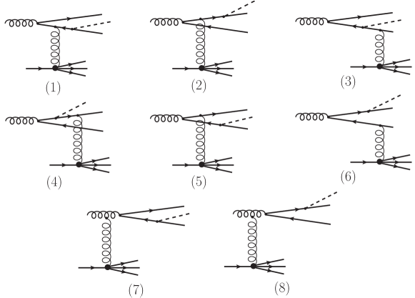
Figure 1: Leading-order gluon-initiated contributions to the inclusive $\bar{Q}QH$ system production in the gluon-proton scattering in the proton rest frame.

Note, the Born-level diagrams are shown in Fig. 1 only for illustration. By the virtue of the color dipole framework, the inclusion of the universal dipole cross section phenomenologically generalises the Born diagrams and effectively resums the lower gluonic ladder diagrams at small x to all orders, similarly to the $k_{\perp}$-factorisation technique. The upper partonic ladder will be accounted via DGLAP evolution of the gluonic density at the NLO.

The kinematics and a detailed derivation of the corresponding amplitude in impact parameter representation are presented in Appendix A. In order to derive the dipole formula for the corresponding process, one should switch to the impact parameter representation performing 2D Fourier transform over the relative transverse momentum between $Q$ and $\bar{Q}$, $\vec{\varkappa}$, total transverse momentum of the $\bar{Q}QH$ system, $\vec{k}_{\perp}$, and the transverse momentum of the Higgs boson, $\vec{\kappa}$, defined in the gluon-target c.m. frame in the limit $\kappa\gg k_{\perp}$ and $\alpha_{3}\ll 1$. The latter differs from the standard Higgs boson transverse momentum defined in proton-target c.m. frame. Corresponding amplitudes in the impact parameter space are

$$A^{\mu\bar{\mu}}_{a}\equiv\int\frac{d^{2}k_{\perp}}{(2\pi)^{2}}\frac{d^{2}\varkappa}{(2\pi)^{2}}\frac{d^{2}\kappa}{(2\pi)^{2}}\,B^{\mu\bar{\mu}}_{a}\,e^{-i\vec{k}_{\perp}\vec{s}-i\vec{\varkappa}\vec{r}-i\vec{\kappa}\vec{\rho}}=3\sum_{d=1}^{N_{c}^{2}-1}\,{\xi_{Q}^{\mu}}^{\dagger}\Big{\{}\tau_{a}\tau_{d}\,\hat{\cal T}^{(d)}_{1}+\tau_{d}\tau_{a}\,\hat{\cal T}^{(d)}_{2}\Big{\}}\tilde{\xi}_{\bar{Q}}^{\bar{\mu}}\,,$$

in terms of the impact parameter dependent amplitudes

$$\hat{\cal T}^{(d)}_{1}(\vec{s},\vec{r},\vec{\rho}) = \hat{\Psi}_{1}(\alpha,\alpha_{3};\vec{r},\vec{\rho})\,\Big{[}\hat{\gamma}^{(d)}(\vec{s}-\alpha\vec{r})-\hat{\gamma}^{(d)}\Big{(}\vec{s}-\alpha\vec{r}-\frac{\alpha_{3}}{\bar{\alpha}}(\vec{\rho}+\alpha\vec{r})\Big{)}\Big{]}\,,$$

$$\hat{\cal T}^{(d)}_{2}(\vec{s},\vec{r},\vec{\rho}) = \hat{\Psi}_{2}(\alpha,\alpha_{3};\vec{r},\vec{\rho})\,\Big{[}\hat{\gamma}^{(d)}(\vec{s}+\bar{\alpha}\vec{r})-\hat{\gamma}^{(d)}\Big{(}\vec{s}+\bar{\alpha}\vec{r}-\frac{\alpha_{3}}{\alpha}(\vec{\rho}-\bar{\alpha}\vec{r})\Big{)}\Big{]}\,.$$

Here, we introduced short-hand notations for the respective production of the wave functions for given scales

$$\hat{\Psi}_{1}(\alpha,\alpha_{3};\vec{r},\vec{\rho}) \equiv \frac{\alpha_{3}}{\bar{\alpha}}\,\hat{\Phi}_{\bar{Q}Q}(\vec{r},m_{Q})\,\hat{\Phi}_{QH}(\vec{\rho}+\alpha\vec{r},\tau)\,,$$ (2)

$$\hat{\Psi}_{2}(\alpha,\alpha_{3};\vec{r},\vec{\rho}) \equiv \frac{\alpha_{3}}{\alpha}\,\hat{\Phi}_{\bar{Q}H}(-\vec{\rho}+\bar{\alpha}\vec{r},\tau)\,\hat{\Phi}_{\bar{Q}Q}(\vec{r},m_{Q})\,,$$ (3)

where $\tau$ is the hard scale determined in Eq. (72), $\tau_{a}$ are the standard $SU(N_{c})$ generators related to the Gell-Mann matrices as $\lambda_{a}=\tau_{a}/2$, and the gluon-target interaction amplitude $\hat{\gamma}^{(d)}(\vec{s})$ is an operator in colour and coordinate space of the target quarks defined as Kopeliovich:2001ee

$$\hat{\gamma}^{(d)}(\vec{s})\equiv\frac{\sqrt{\alpha_{s}}}{\sqrt{6}}\,\int\frac{d^{2}k_{\perp}}{(2\pi)^{2}}\,\frac{\hat{F}^{(d)}_{Gp\to X}(\vec{k}_{\perp},\{X\})}{\vec{k}_{\perp}^{2}+m_{g}^{2}}\;e^{-i\vec{k}_{\perp}\vec{s}}=\sum_{j}\tau^{(j)}_{a}\chi(\vec{s}-\vec{b}_{j})\,.$$ (4)

Here, $\chi(\vec{s}-\vec{b}_{j})$ is the interaction amplitude of projectile heavy quark with $j$-th constituent valence quark in the target proton, $\vec{s}$ is the transverse distance between projectile heavy quark and the center of gravity of the target, $\vec{b}_{j}$ the transverse distance between $j$-th constituent valence quark in the target and the center of gravity of the target.

The $G_{a}\to Q\bar{Q}$ and $Q/\bar{Q}\to Q/\bar{Q}+H$ distribution amplitudes in impact parameter representation read

$$\hat{\Phi}_{\bar{Q}Q}(\vec{r},\epsilon) \equiv \int\frac{d^{2}\varkappa}{(2\pi)^{2}}\,\hat{\Theta}_{\bar{Q}Q}(\vec{\varkappa},\epsilon)\,e^{-i\vec{\varkappa}\vec{r}}$$

$$= \frac{\sqrt{\alpha_{s}}}{(2\pi)\sqrt{2}}\,\Big{\{}m_{Q}(\vec{e}\cdot\vec{\sigma})+i(1-2\alpha)(\vec{\sigma}\cdot\vec{n})(\vec{e}\cdot\vec{\nabla}_{r})-(\vec{e}\times\vec{n})\cdot\vec{\nabla}_{r}\Big{\}}\,K_{0}(\epsilon\,r)\,,$$

$$\hat{\Phi}_{QH}(\vec{\rho},\varepsilon) \equiv \int\frac{d^{2}\kappa}{(2\pi)^{2}}\,\hat{\Theta}_{QH}(\vec{\kappa},\varepsilon)\,e^{-i\vec{\kappa}\vec{\rho}}=\frac{m_{Q}}{(2\pi)\sqrt{3\pi}v}\,\Big{\{}2m_{Q}\,\vec{\sigma}\cdot\vec{n}+\,\vec{\sigma}\cdot\vec{\nabla}_{\rho}\Big{\}}\,K_{0}(\varepsilon\,\rho)\,,$$ (6)

$$\hat{\Theta}_{\bar{Q}Q}(\vec{\varkappa},\epsilon) \equiv \frac{\sqrt{\alpha_{s}}}{\sqrt{2}}\,\frac{\hat{U}(\vec{\varkappa})}{\vec{\varkappa}^{2}+\epsilon^{2}}\,,\qquad\hat{\Theta}_{QH}(\vec{\kappa},\varepsilon)\equiv\frac{m_{Q}}{\sqrt{3\pi}v}\,\frac{\hat{V}(\gamma)}{\vec{\kappa}^{2}+\varepsilon^{2}}\,,$$ (7)

respectively, where $\hat{V}(\gamma)$ ($\gamma=\alpha_{3}/\bar{\alpha}$ or $\alpha_{3}/\alpha$) and $\hat{U}(\vec{\varkappa})$ are defined in Eq. (66), $r\equiv|\vec{r}|$ and $\rho\equiv|\vec{\rho}|$. When taking square of the total inclusive $G_{a}+p\to Q\bar{Q}H+X$ amplitude in impact parameter representation

$$\overline{|A|^{2}}(\vec{r}_{1},\vec{\rho}_{1};\vec{r}_{2},\vec{\rho}_{2})\equiv\int d^{2}s\,d\{X\}\sum_{\lambda_{*},a,\mu,\bar{\mu}}\langle A^{\mu\bar{\mu}}_{a}(\vec{r}_{1},\vec{\rho}_{1})\big{(}A^{\mu\bar{\mu}}_{a}\big{)}^{\dagger}(\vec{r}_{2},\vec{\rho}_{2})\rangle_{|3q\rangle_{1}}$$ (8)

one implicitly performs an averaging over colour indices and polarisation $\lambda_{*}$ of the incoming projectile gluon $G_{a}$ in the $G_{a}\to Q\bar{Q}$ and $Q/\bar{Q}\to Q/\bar{Q}+H$ distribution amplitudes as well as over valence quarks and their relative coordinates in the target proton $|3q\rangle_{1}$. Besides, one uses the general properties of the 2-spinors

$$\sum_{\mu,\bar{\mu}}\tilde{\xi}_{\bar{Q}}^{\bar{\mu}}\big{(}{\xi_{Q}^{\mu}}^{\dagger}\big{)}^{*}=\hat{1}\,,\qquad\sum_{\mu,\bar{\mu}}\big{(}{\xi_{Q}^{\mu}}^{\dagger}\hat{a}\tilde{\xi}_{\bar{Q}}^{\bar{\mu}}\big{)}^{*}\,\big{(}{\xi_{Q}^{\mu}}^{\dagger}\hat{b}\tilde{\xi}_{\bar{Q}}^{\bar{\mu}}\big{)}={\rm Tr}\big{(}\hat{a}^{\dagger}\hat{b}\big{)}\,.$$ (9)

Then, squaring the operator $\hat{\gamma}^{(d)}$ and then averaging it over quark positions and quantum numbers the initial nucleon wave function $|3q\rangle_{1}$ and summing over the final $\{X\}$ leads to

$$\int d\{X\}\langle i|\hat{\gamma}_{a}(\vec{s}_{k})\hat{\gamma}^{\dagger}_{a^{\prime}}(\vec{s}_{l})|i\rangle_{|3q\rangle_{1}}=\frac{1}{8}\,\delta_{aa^{\prime}}\,S(\vec{s}_{k},\vec{s}_{l})\,,$$ (10)

where the colour averaging procedure

$$\langle i|\tau_{a}^{(j)}\cdot\tau_{a^{\prime}}^{(j^{\prime})}|i\rangle_{|3q\rangle_{1}}=\left\{\begin{array}[]{lr}\frac{1}{6}\delta_{aa^{\prime}}&:j=j^{\prime}\\ -\frac{1}{12}\delta_{aa^{\prime}}&:j\not=j^{\prime}\end{array}\right.$$ (13)

has been performed, and $S(\vec{s}_{k},\vec{s}_{l})$ is the scalar function given by

$$S(\vec{s}_{k},\vec{s}_{l}) \equiv \frac{2}{9}\int d\{b\}\Big{[}\sum_{j=1}^{3}\chi(\vec{s}_{k}-\vec{b}_{j})\chi(\vec{s}_{l}-\vec{b}_{j})$$

$$- \frac{1}{2}\sum_{j\not=j^{\prime}}\chi(\vec{s}_{k}-\vec{b}_{j})\chi(\vec{s}_{l}-\vec{b}_{j^{\prime}})\Big{]}\,|\Phi_{|3q\rangle_{1}}(\{\vec{b}\})|\,.$$

in terms of the quark-target scattering amplitude, $\chi(\vec{R})$, and the proton wave function, $\Phi_{|3q\rangle_{1}}\{\vec{b}\}$. This function is directly related to the universal $q\bar{q}$ dipole cross section known from phenomenology as follows

$$\sigma_{\bar{q}q}(\vec{s}_{1}-\vec{s}_{2})\equiv\int d^{2}s\Big{[}S(\vec{s}+\vec{s}_{1},\vec{s}+\vec{s}_{1})+S(\vec{s}+\vec{s}_{2},\vec{s}+\vec{s}_{2})-2S(\vec{s}+\vec{s}_{1},\vec{s}+\vec{s}_{2})\Big{]}\,.$$ (14)

The universal dipole cross section $\sigma_{\bar{q}q}$ implicitly depends on energy. Although being universal, it cannot be calculated reliably from the first principles, but is known from phenomenology. A popular simple GBW ansatz for the saturated shape of the dipole cross section with $x_{2}$-dependent parameters fitted to the HERA hard DIS data at small $x$ GBWdip

$$\sigma_{\bar{q}q}(\vec{R})=\bar{\sigma}_{0}\Big{[}1-e^{-\vec{R}^{2}/\bar{R}_{0}^{2}(x_{2})}\Big{]}$$ (15)

is sufficient for our purposes here since the typical hard scale of inclusive Higgsstrahlung is large, i.e. $\mu\sim M\gg m_{g}$, and thus all the incident dipole sizes are small compared to the hadron scale (the latter is not true for diffraction, see below). In this case, due to the colour transparency property it suffices to use

$$\sigma_{\bar{q}q}(\vec{R})\simeq\frac{\bar{\sigma}_{0}}{\bar{R}_{0}^{2}(x_{2})}\;\vec{R}^{2}\,,\qquad R\ll\bar{R}_{0}(x_{2})\,,$$ (16)

to the first approximation. The GBW fits provide

$$\bar{\sigma}_{0}=23.03\;\mathrm{mb}\,,\qquad\bar{R}_{0}(x)=0.4\,\mathrm{fm}\times(x/x_{0})^{0.144}\,,\qquad x_{0}=3.04\times 10^{-4}\,.$$ (17)

Following to the above scheme one obtains the amplitude squared $\overline{|A|^{2}}$ in an analytic form as a linear combination of the dipole cross sections for different dipole separations, with coefficients given by colour structure and distribution amplitudes. The dipole formula for the differential cross section of the $G_{a}+p\to\bar{Q}QH+X$ process then reads

$$\frac{d\sigma(Gp\to\bar{Q}QH+X)}{d\alpha d\ln\alpha_{3}}=\int d^{2}rd^{2}\rho\;\overline{|A|^{2}}(\vec{r},\vec{\rho})\,,$$ (18)

Here, the amplitude squared in the general form

$$\overline{|A|^{2}}(\vec{r},\vec{\rho})=\frac{3}{8}(\Psi_{1}\Psi_{2}^{\dagger}+\Psi_{2}\Psi_{1}^{\dagger})\,\sigma_{\rm eff}(\vec{r},\vec{R}_{1},-\vec{R}_{2})+\,6\big{(}\Psi_{1}\Psi_{1}^{\dagger}\,\sigma_{\bar{q}q}(\vec{R}_{1})+\Psi_{2}\Psi_{2}^{\dagger}\,\sigma_{\bar{q}q}(\vec{R}_{2})\big{)}\,,$$

where

$$\sigma_{\rm eff}(\vec{l}_{1},\vec{l}_{2},\vec{l}_{3})\equiv\sigma_{\bar{q}q}(\vec{l}_{1})-\sigma_{\bar{q}q}(\vec{l}_{1}+\vec{l}_{3})-\sigma_{\bar{q}q}(\vec{l}_{1}+\vec{l}_{2})+\sigma_{\bar{q}q}(\vec{l}_{1}+\vec{l}_{2}+\vec{l}_{3})\,,$$

$$\vec{R}_{1}\equiv\frac{\alpha_{3}}{\bar{\alpha}}\,(\vec{\rho}+\alpha\vec{r})\,,\quad\vec{R}_{2}\equiv\frac{\alpha_{3}}{\alpha}\,(\vec{\rho}-\bar{\alpha}\vec{r})\,.$$ (19)

Transition to the hadron level is usually performed as follows (see e.g. Ref. Kopeliovich:2001ee )

$$\frac{d\sigma_{\rm incl}}{dY\,d\alpha\,d\ln\alpha_{3}}=G(x_{1},\mu^{2})\,\frac{d\sigma(Gp\to\bar{Q}QH+X)}{d\alpha d\ln\alpha_{3}}\,,$$ (20)

where the projectile gluon distribution in the incoming proton is treated via the collinear factorisation technique, $Y$ is the rapidity of the $\bar{Q}QH$ system, and

$$G(x_{1},\mu^{2})\equiv x_{1}g(x_{1},\mu^{2})\,,\qquad x_{1,2}=\frac{M}{\sqrt{s}}\,e^{\pm Y}\,.$$ (21)

are the collinear gluon density at the hard scale $\mu^{2}\simeq M^{2}$ being the invariant mass of the $Q\bar{Q}H$ system defined in Eq. (70) and the momentum fractions of the projectile and $t$-channel gluon, respectively.

Figure 2: The differential Higgs boson transverse momentum $\kappa$ distribution of the inclusive Higgsstrahlung obtained via the asymptotic dipole formula (22) valid in the limit of small $k_{\perp}\ll\varkappa,\,\kappa$ and $\alpha_{3}\ll 1$ in comparison to the exact result of $k_{\perp}$-factorisation from Ref. Lipatov:2009qx .

In order to obtain the Higgsstrahlung cross section differential in relative transverse momenta $\vec{\kappa}$ and $\vec{\varkappa}$, one can directly use the asymptotic amplitudes (73) and (73) in the limit of small $k_{\perp}\ll\varkappa,\,\kappa$. At the level of cross section, this asymptotics is equivalent to taking the first quadratic term in the dipole cross section (16). In this case, we obtain the fully differential inclusive Higgsstrahlung cross section which reads

$$\frac{d\sigma_{\rm incl}}{d\Omega}\simeq\frac{1}{(2\pi)^{4}}\,\frac{3\bar{\sigma}_{0}}{4\bar{R}_{0}^{2}(x_{2})}\,g(x_{1},\mu^{2})\;\mathrm{Tr}\Big{[}8\vec{\hat{{\cal K}}}_{1}\cdot\vec{\hat{{\cal K}}}^{\dagger}_{1}+8\vec{\hat{{\cal K}}}_{2}\cdot\vec{\hat{{\cal K}}}^{\dagger}_{2}-\vec{\hat{{\cal K}}}_{1}\cdot\vec{\hat{{\cal K}}}^{\dagger}_{2}-\vec{\hat{{\cal K}}}_{2}\cdot\vec{\hat{{\cal K}}}^{\dagger}_{1}\Big{]}\,,$$ (22)

where $\vec{\hat{{\cal K}}}_{1,2}$ are defined in terms of momentum-space wave functions (7) as

$$\vec{\hat{{\cal K}}}_{1} \equiv -\frac{\alpha_{3}}{\bar{\alpha}}\,\hat{\Theta}_{\bar{Q}Q}(\vec{\varkappa}-\alpha\vec{\kappa},m_{Q})\,\frac{\partial}{\partial\vec{z}}\Big{[}\hat{\Theta}_{QH}(\vec{z},\tau)\Big{]}_{\vec{z}=\vec{\kappa}}\,,$$ (23)

$$\vec{\hat{{\cal K}}}_{2} \equiv \frac{\alpha_{3}}{\alpha}\,\frac{\partial}{\partial\vec{z}}\Big{[}\hat{\Theta}_{QH}(\vec{z},\tau)\Big{]}_{\vec{z}=-\vec{\kappa}}\,\hat{\Theta}_{\bar{Q}Q}(\vec{\varkappa}+\bar{\alpha}\vec{\kappa},m_{Q})\,,$$ (24)

and

$$d\Omega\equiv dx_{1}\,d\alpha\,d\ln\alpha_{3}\,d^{2}\varkappa\,d^{2}\kappa$$ (25)

is the element of the phase space volume associated with the produced system $\bar{Q}QH$. The remaining momentum integrals can then be numerically evaluated over a given phase space volume specific to a given measurement (see below).

In Fig. 2 the approximated dipole formula result for the inclusive Higgsstrahlung cross section differential in Higgs boson transverse momentum $\kappa$ (22) is compared to the corresponding exact calculation in the $k_{\perp}$-factorisation approach of Ref. Lipatov:2009qx . Remind, the asymptotic dipole formula Eq. (22) is obtained in the collinear projectile gluon and soft target gluon $k_{\perp}\ll\varkappa,\,\kappa$ approximations, as well as for $\alpha_{3}\ll 1$. In this case, the final Higgs boson transverse momentum is entirely generated by a recoil against heavy quarks in the final state. Besides, the Higgs boson is assumed to take only a relatively small fraction of the quark momenta. A comparison with the exact result of Ref. Lipatov:2009qx shows that the asymptotic Higgs boson spectrum (22) generated by purely final state kinematics dominates the total cross section at large Higgs boson transverse momenta $\kappa\gtrsim m_{H}$ and approaches the exact result both in shape and normalisation. At lower transverse momenta, however, we notice a missing strength due to the omitted diagrams as well as a potentially large role of the non-Gaussian tail in primordial gluon transverse momenta distribution. The latter should be accounted for by the use of unintegrated gluon distribution functions as was done in Ref. Lipatov:2009qx .

On the other hand, the simplified dipole formula (20) with a collinear starting PDF (21) and the quadratic approximation in the dipole cross section (16) will enable us to calculate the SD-to-inclusive ratio in a fully analytic form which does not depend on higher order QCD corrections and on projectile gluon evolution and is given only in terms of parameters of the universal dipole cross section (see below). As will be discussed below, the ratio is not sensitive to the high-$p_{T}$ approximation we adopted in the analysis of the absolute cross sections as well as to the short-distance corrections to the $gg\to Q\bar{Q}H$ subprocess. It therefore can be applied to the conventional NNLO+NNLL $Q\bar{Q}H$ inclusive cross sections and/or those obtained in the $k_{\perp}$ factorisation approach known from the literature in order to get a good first estimate of the diffractive Higgsstrahlung cross section.

III Single diffractive Higgsstrahlung in the dipole picture

When it comes to diffraction, the QCD factorisation in hadronic collisions is severely broken by the interplay of soft and hard QCD interactions and by the absorptive effects Kopeliovich:2006tk ; Pasechnik:2011nw . While the former mechanism, which is the leading twist, is frequently missed, the latter effect is modelled by the gap survival probability factor, which is usually applied to correct the factorisation-based results. A successful alternative to the factorisation-based parton model, the colour dipole description zkl goes beyond the QCD factorisation and naturally accounts for the hard-soft QCD dynamics interplay, and for the absorptive effects at the amplitude level (see e.g. Refs. Kopeliovich:2007vs ; Pasechnik:2012ac ). The single diffractive $Q\bar{Q}+H$ production (with the leading proton and a rapidity gap) is not yet available in the literature, and this Section is devoted to the corresponding analysis in the dipole approach.

III.1 Diffractive amplitude

In order to derive the single diffractive Higgsstrahlung amplitude in impact parameter representation we refer to the corresponding framework previously developed for diffractive gluon radiation and diffractive DIS processes in Refs. GBWdip ; Raufeisen:2002zp ; kst1 and we adopt similar notations in what follows. Similarly to the inclusive case considered above, we are interested in single-diffractive Higgsstrahlung at high energies when the Higgs boson takes relatively small fraction of the heavy quark momentum since the well-known wave functions for $G\to Q\bar{Q}$ and $Q(\bar{Q})\to Q(\bar{Q})+H$ are factorized out in the impact parameter space. The latter situation thus enables us to employ the dipole approach in this first study of the diffractive Higgsstrahlung process.

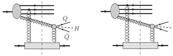
Figure 3: The dominating gluon-initiated contributions to the single diffractive $\bar{Q}Q+H$ production in $pp$ collisions. The hard $G_{a}+p\to\bar{Q}QH+X$ subprocess via single gluon exchange where all possible di-gluon couplings to $Q\bar{Q}H$ system are resummed and denoted by filled grey circle and explicitly described in Fig. 1. The unitarity cut between the $t$-channel “active” (rightmost gluon) and “screening” (leftmost gluon) exchanges is shown by vertical dashed line. In actual calculations, we adopt the Good-Walker picture of diffraction GW (see main text).

For illustration, the dominating parton-level gluon-initiated graphs are shown in Fig. 3 where we account only for the diagrams where the “active” gluon is coupled to the hard $Q\bar{Q}+H$ system, while the soft “screening” gluon couples to a spectator parton at a large impact distance. Other diagrams where both “active” and “screening” gluons couple to partons at small relative distances are the higher twist ones and thus are strongly suppressed by extra powers of the hard scale $\mu^{2}\sim M^{2}$ (see e.g. Refs. Kopeliovich:2007vs ; Pasechnik:2012ac ). This becomes even more obvious in the colour dipole framework due to colour transparency zkl making the medium more transparent for smaller dipoles.

In what follows, we do not explicitly calculate the Feynman graphs in Fig. 3 but instead adopt the Good-Walker picture of diffraction GW where a diffractive scattering amplitude is proportional to a difference between elastic scatterings of different Fock states off the target in the target rest frame. To this end, applying the generalized optical theorem in the high energy limit with a cut between the “screening” and “active” $t$-channel gluons as illustrated in Fig. 3, we write

$$\hat{A}^{a}_{\rm SD}(\vec{r}_{1},\vec{r}_{2},\vec{r}_{3})=\frac{i}{2}\sum_{Y^{*}}\langle{\rm in}|(A^{\mu\bar{\mu}}_{a})^{\dagger}|Y^{*}\rangle\langle Y^{*}|A_{\rm scr}(\vec{r}_{1},\vec{r}_{2},\vec{r}_{3})|{\rm in}^{\prime}\rangle,$$ (26)

where $A_{\rm scr}$ is the “screening gluon” exchange amplitude between a constituent (valence) projectile quark and the target, $A^{\mu\bar{\mu}}_{a}$ is the “active gluon” exchange amplitude between colour-singlet $G_{a}(\bar{Q}Q)H$ system and the target found earlier. In the above equation, summation goes through all the intermediate states $\{Y^{*}\}$ except the projectile gluon $G_{a}$, and $a$ is the colour index of the projectile gluon $G_{a}$. The latter gluon can be assumed to be decoherent in colour w.r.t. valence quarks in the incoming proton wave function and thus its colour should be summed up independently of the “screening” $A_{\rm scr}$ amplitude at the level of cross section.

Indeed, the projectile hard gluon before its splitting to $Q\bar{Q}H$ system in the colour field of the target undergoes multiple radiation steps $g\to gg$ populating the forward rapidity domain with gluon radiation with momenta below the hard scale of the process $p_{\perp}^{rad}<\mu$. The radiated gluons should then be resummed and can be taken into account by using the corresponding gluon PDF similarly to the inclusive case considered above. Since the hard gluon experiences many splittings on its way (e.g. radiates many gluons and quarks) before it gives rise to the $\bar{Q}Q+H$ system, naturally its colour gets completely uncorrelated with the colour of the parent valence quark, which should be taken into account in the respective colour averaging procedure. So in the single diffractive amplitude squared one effectively sums over the projectile gluon colour as follows

$$\overline{|A_{\rm SD}|^{2}}=\sum_{a=1}^{N_{c}^{2}-1}\langle\hat{A}^{a}_{\rm SD}(\hat{A}^{a}_{\rm SD})^{\dagger}\rangle_{|3q\rangle_{1}}\,,$$ (27)

where the averaging over the colours of the constituent quarks in the incoming proton wave function $|3q\rangle$ is implicitly performed according to the rule

$$\langle\hat{A}\big{(}\tau^{(1)}\big{)}\hat{B}\big{(}\tau^{(2)}\big{)}\hat{C}\big{(}\tau^{(3)}\big{)}\rangle_{|3q\rangle_{1}} = \frac{1}{6}\Big{\{}{\rm Tr}\,\hat{A}(\tau)\;{\rm Tr}\,\hat{B}(\tau)\;{\rm Tr}\,\hat{C}(\tau)+{\rm Tr}\Big{[}\hat{A}\big{(}\tau\big{)}\hat{B}\big{(}\tau\big{)}\hat{C}\big{(}\tau\big{)}\Big{]}$$

$$+ {\rm Tr}\Big{[}\hat{A}\big{(}\tau\big{)}\hat{C}\big{(}\tau\big{)}\hat{B}\big{(}\tau\big{)}\Big{]}-{\rm Tr}\,\hat{A}\big{(}\tau\big{)}\,\Big{[}\hat{B}\big{(}\tau\big{)}\hat{C}\big{(}\tau\big{)}\Big{]}$$

$$- {\rm Tr}\,\hat{B}\big{(}\tau\big{)}\,\Big{[}\hat{A}\big{(}\tau\big{)}\hat{C}\big{(}\tau\big{)}\Big{]}-{\rm Tr}\,\hat{C}\big{(}\tau\big{)}\,\Big{[}\hat{A}\big{(}\tau\big{)}\hat{B}\big{(}\tau\big{)}\Big{]}\Big{\}}\,,$$

where $\hat{A}\big{(}\tau^{(1)}\big{)}$, $\hat{B}\big{(}\tau^{(2)}\big{)}$, and $\hat{C}\big{(}\tau^{(3)}\big{)}$ are arbitrary functions of $\tau^{(j)}$ matrices corresponding to valence quarks with $j=1,2,3$ in the projectile proton, respectively.

It is well-known that the gluons in such a gluonic ladder are predominantly located in a close vicinity of the valence quarks in the so-called “gluonic spots” which have mean size of about $\sim 0.3$ fm KST-par ; spots . Thus, to the first approximation one could neglect the distance between the projectile gluon $G_{a}\to\bar{Q}Q+H$ and the closest constituent quark compared to the typical distances between the constituent quarks $\sim 1$ fm. Then, the amplitude of the “screening gluon” exchange summed over projectile valence quarks $j=1,2,3$ reads

$$A^{(i)}_{\rm scr}(\vec{r}_{1},\vec{r}_{2},\vec{r}_{3})=\sum_{j\not=i,d^{\prime}}\tau^{(j)}_{d^{\prime}}\big{\{}\hat{\gamma}_{d^{\prime}}(\vec{r}_{i})-\hat{\gamma}_{d^{\prime}}(\vec{r}_{i}+\vec{r}_{ij})\big{\}}\,,$$ (28)

where $\vec{r}_{1}$ is the impact parameter of the gluon $G_{a}$ or the closest constituent quark $q_{i}$ (the gluon $G_{a}$ is assumed to belong to one of the three “gluonic spots” in the projectile proton), $\vec{r}_{ij}\equiv\vec{r}_{j}-\vec{r}_{i}$ is the distances of the other two constituent quark $q_{j}$, $j\not=i$ from the $q_{i}$ quark, and the matrices $\hat{\gamma}_{a}$ are the operators in coordinate and colour space for the target quarks defined in Eq. (4). Due to the colour transparency, the soft amplitude (28) naturally vanishes if all the distances in the projectile proton disappear, i.e. $\vec{r}_{ij}\to 0$. Finally, one should sum over contributions from the valence quarks (or the corresponding “spots”), i.e.

$$A_{\rm scr}(\vec{r}_{1},\vec{r}_{2},\vec{r}_{3})=\sum_{i=1}^{3}A^{(i)}_{\rm scr}\,,$$ (29)

which is equivalent to accounting for cyclic permutation of the valence quarks at the amplitude level.

In what follows, it is convenient to choose the following set of independent variables

$$\{\vec{r}_{1},\;\vec{r}_{2},\;\vec{r}_{3}\}\qquad\Rightarrow\qquad\{\vec{s},\;\vec{r}_{12},\;\vec{r}_{13}\}$$ (30)

where $\vec{s}$ is the impact parameter of the projectile gluon $G_{a}$. In variance with the inclusive case considered above, the diffractive scattering is very sensitive to the typical hadron size in the projectile proton, i.e. large hadron-scale dipoles $|\vec{r}_{ij}|\sim b\sim R_{p}$, $i\not=j$ ($R_{p}$ is the mean proton size) become important and control the diffractive Higgsstrahlung. In this case the Bjorken variable $x$ is ill defined, and a more appropriate variable is the $pp$ collisions energy. An energy dependent parametrization of the dipole cross section with the same saturated shape as in the GBW case (15)

$$\sigma_{\bar{q}q}(\vec{R},\hat{s})=\sigma_{0}(\hat{s})\Big{[}1-e^{-\vec{R}^{2}/R_{0}^{2}(\hat{s})}\Big{]}\,,\qquad$$ (31)

with parameters being functions of the gluon-target c.m. energy squared $\hat{s}=x_{1}s$ ($s$ is $pp$ c.m. energy squared),

$$R_{0}(\hat{s})=0.88\,\mathrm{fm}\,(s_{0}/\hat{s})^{0.14}\,,\quad\sigma_{0}(\hat{s})=\sigma_{tot}^{\pi p}(\hat{s})\Big{(}1+\frac{3R_{0}^{2}(\hat{s})}{8\langle r_{ch}^{2}\rangle_{\pi}}\Big{)}\,,$$ (32)

was proposed and fitted to the soft hadronic data in Ref. KST-par . Here, the pion-proton total cross section is parametrized as barnett $\sigma_{tot}^{\pi p}(\hat{s})=23.6(\hat{s}/s_{0})^{0.08}$ mb, $s_{0}=1000\,\,\mbox{GeV}^{2}$, the mean pion radius squared is amendolia $\langle r_{ch}^{2}\rangle_{\pi}=0.44$ fm².

Following the above scheme one obtains the diffractive Higgsstrahlung amplitude $\hat{A}^{a}_{\rm SD}$ in analytic form as a linear combination of the dipole cross sections for different dipole separations. As was anticipated, the diffractive amplitude represents the destructive interference effect from scattering of dipoles of slightly different sizes and vanishes as $\hat{A}^{a}_{\rm SD}\propto\alpha_{3}^{2}$ in the limit $\alpha_{3}\to 0$. Such an interference results in the interplay between hard and soft fluctuations in the diffractive $pp$ amplitude, enhancing the breakdown of diffractive factorisation Kopeliovich:2006tk ; Pasechnik:2011nw .

III.2 The dipole formula for the cross section

Note that initial $\langle{\rm in}|$ and intermediate $|Y^{*}\rangle$ states are composite and contain the projectile proton wave function of the initial proton $\Psi_{i}(\vec{r}_{l},x_{l})$ and the projectile proton remnant wave function $\Psi_{f}(\vec{r}_{l},x_{l})$ as a function of positions $\vec{r}_{i}$ and momentum fractions $x_{i}$ of all the incident partons. Using the squaring rule for gluon-target interactions given by Eq. (10), integrating over $\vec{s}$ according to Eq. (14), keeping only the leading (quadratic) terms in small $\rho,r\ll r_{ij}$ and Fourier-transforming the amplitude back to momentum space, we obtain explicitly

$$\overline{|A_{\rm SD}|^{2}} \simeq \frac{3}{256}\,|\Psi_{in}|^{2}\,|\Psi_{fin}|^{2}\,\sum_{i,j=1}^{2}\Omega^{ij}_{\rm hard}\,\Omega^{ij}_{\rm soft}\,,$$

$$\Omega^{ij}_{\rm hard} = \mathrm{Tr}\Big{[}8\hat{{\cal K}}_{1,i}\hat{{\cal K}}^{\dagger}_{1,j}+8\hat{{\cal K}}_{2,i}\hat{{\cal K}}^{\dagger}_{2,j}-\hat{{\cal K}}_{1,i}\hat{{\cal K}}^{\dagger}_{2,j}-\hat{{\cal K}}_{2,i}\hat{{\cal K}}^{\dagger}_{1,j}\Big{]}\,,$$

$$\Omega^{ij}_{\rm soft} = \Big{\{}\big{[}2\nabla_{i}\sigma_{\bar{q}q}(\vec{r}_{12})+\nabla_{i}\sigma_{\bar{q}q}(\vec{r}_{12}-\vec{r}_{13})+\nabla_{i}\sigma_{\bar{q}q}(\vec{r}_{13})\big{]}\nabla_{j}\sigma_{\bar{q}q}(\vec{r}_{12})$$ (33)

$$+ \big{[}\nabla_{i}\sigma_{\bar{q}q}(\vec{r}_{12})+2\nabla_{i}\sigma_{\bar{q}q}(\vec{r}_{12}-\vec{r}_{13})-\nabla_{i}\sigma_{\bar{q}q}(\vec{r}_{13})\big{]}\nabla_{j}\sigma_{\bar{q}q}(\vec{r}_{12}-\vec{r}_{13})$$

$$+ \big{[}\nabla_{i}\sigma_{\bar{q}q}(\vec{r}_{12})-\nabla_{i}\sigma_{\bar{q}q}(\vec{r}_{12}-\vec{r}_{13})+2\nabla_{i}\sigma_{\bar{q}q}(\vec{r}_{13})\big{]}\nabla_{j}\sigma_{\bar{q}q}(\vec{r}_{13})\Big{\}}\,,$$

where $\vec{\hat{{\cal K}}}_{1,2}$ are defined earlier in Eqs. (23) and (24),

$$\nabla_{i}\sigma_{\bar{q}q}(\vec{R})=\frac{2\sigma_{0}(\hat{s})}{R_{0}^{2}(\hat{s})}\,R_{i}\,e^{-R^{2}/R_{0}^{2}(\hat{s})}\,,$$ (34)

with the saturated form of the dipole cross section in the KST (energy dependent) form (31) and (32). Equation (33) corresponds to the single diffractive $\bar{Q}QH$ production process in the Good-Walker picture GW , by construction. We notice that the soft ($r_{ij}$-dependent) part of the SD amplitude squared in Eq. (33) has been accumulated in $\Omega^{ij}_{\rm soft}$ while all the dependence on the hard scales $\rho$ and $r$ is contained in $\Omega^{ij}_{\rm hard}$, while the partonic structure of the projectile proton is concentrated in $|\Psi_{in}|^{2}$. The amplitude above is normalized in such a way that the cross section of the $\bar{Q}Q+H$ production in forward single-diffractive $pp$ scattering reads

$$\frac{d\sigma_{\rm SD}}{d\alpha\,d\ln\alpha_{3}\,d^{2}\delta_{\perp}}\Big{|}_{\delta_{\perp}\to 0}=\frac{1}{(2\pi)^{2}}\,\int\prod_{i,j}d^{2}r_{i}d^{2}r^{\prime}_{j}\,\prod_{k,l,m,n}dx_{q}^{k}dx_{g}^{l}dx_{q}^{\prime m}dx_{g}^{\prime n}\,\int d^{2}rd^{2}\rho\,\overline{|A_{\rm SD}|^{2}}\,,$$ (35)

where $\vec{\delta}_{\perp}$ is the transverse momentum of the final proton associated with the $t$-channel momentum transfer squared, $t=-|\delta_{\perp}|^{2}$, $x_{q/g}^{i}$ are the fractional light-cone momenta of the valence/sea quarks and gluons. As long as the forward diffractive cross section (35) is known, the total SD cross section can be evaluated as

$$\frac{d\sigma_{\rm SD}}{d\Omega}\simeq\frac{1}{B_{\rm SD}(s)}\,\frac{d\sigma_{\rm SD}}{d\Omega\,d\delta_{\perp}}\Big{|}_{\delta_{\perp}\to 0}\,,\quad B_{\rm SD}(s)\simeq\langle r_{ch}^{2}\rangle_{p}/3+2\alpha^{\prime}_{{I\!\!P}}\ln(s/s_{1})\,,\quad s_{1}=1\,{\rm GeV}^{2}$$ (36)

where $d\Omega$ is the element of the phase space volume defined in Eq. (25), and $B_{\rm SD}(s)$ is the Regge-parameterised $t$-slope of the differential SD cross section (with $\alpha^{\prime}_{{I\!\!P}}=0.25\,\,\mbox{GeV}^{-2}$), which is expected to be similar to the $t$-slope measured in diffractive DIS.

The initial proton $\Psi_{in}$ and proton remnant $\Psi_{fin}$ wave functions in Eq. (33) encode information about kinematics and probability distributions of individual (incoming and outgoing) partons. In the unobservable part, the completeness relation to the wave function of the proton remnant $\Psi_{fin}$ in the final state reads

$$\sum_{fin}\Psi_{fin}(\vec{r}_{1},\vec{r}_{2},\vec{r}_{3};\{x_{q}^{1,2,...}\},\{x_{g}^{1,2,...}\})\Psi^{*}_{fin}(\vec{r}\,^{\prime}_{1},\vec{r}\,^{\prime}_{2},\vec{r}\,^{\prime}_{3};\{{x^{\prime}}_{q}^{1,2,...}\},\{{x^{\prime}}_{g}^{1,2,...}\})$$

$$\phantom{.......}=\,\delta\bigl{(}\vec{r}_{1}-\vec{r}\,^{\prime}_{1}\bigr{)}\delta(\vec{r}_{2}-\vec{r}\,^{\prime}_{2})\delta(\vec{r}_{3}-\vec{r}\,^{\prime}_{3})\prod_{j}\delta(x_{q/g}^{j}-{x^{\prime}}_{q/g}^{j})\,.$$ (37)

In the above formula, $\delta$-functions reflect momentum conservation and will simplify the phase space integrations over the unobservable variables in the single diffractive Higgsstrahlung cross section considerably (see below).

The light-cone partonic wave function of the initial proton $\Psi_{in}$ depends on transverse coordinates and fractional momenta of all valence and sea quarks and gluons. As was mentioned above, we assume that the mean transverse distance between a source valence quark and the sea quarks or gluons is much smaller than the mean distance between the valence quarks. Therefore, the transverse positions of sea quarks and gluons can be identified with the coordinates of the valence quarks, and the proton wave function squared $|\Psi_{in}|^{2}$ can be parametrized as,

$$|\Psi_{in}|^{2} = \frac{3a^{2}}{\pi^{2}}e^{-a(r_{1}^{2}+r_{2}^{2}+r_{3}^{2})}\;{\cal R}\big{(}x_{1},\{x_{q}^{1,2,...}\},\{x_{g}^{2,3,...}\}\big{)}$$ (38)

$$\times \delta(\vec{r}_{1}+\vec{r}_{2}+\vec{r}_{3})\delta\Big{(}1-x_{1}-\sum_{j}x_{q/g}^{j}\Big{)},$$

where $a\equiv\langle r_{ch}^{2}\rangle_{p}^{-1}$ is the inverse proton mean charge radius squared, the variable $x_{g}^{1}\equiv x_{1}$ is defined as the light-cone momentum fraction of the hard gluon related to rapidity $Y$ of the produced $\bar{Q}Q+H$ system in Eq. (21); ${\cal R}$ is a valence/sea (anti)quark distribution function in the projectile proton. For simplicity, we parametrize the valence part of the proton wave function in the form of symmetric Gaussian for the spacial quark distributions. Notice that ${\cal R}$ distribution has a low (hadronic) scale, so the constituent quarks, i.e. the valence quarks together with the sea and gluons they generate, carry the whole momentum of the proton, by construction.

In the case of diffractive gluon excitations, after integration over the fractional momenta of all partons not participating in the hard interaction, we arrive at a single gluon distribution in the proton, probed by the heavy system $M$,

$$\int\prod_{j}dx_{q}^{j}\prod_{k\not=1}dx_{g}^{k}\,\delta\Big{(}1-x_{1}-\sum_{l}x_{q/g}^{l}\Big{)}\;{\cal R}\big{(}x_{1},\{x_{q}^{1,2,...}\},\{x_{g}^{2,3,...}\}\big{)}=\Big{(}\frac{C_{A}}{C_{F}}\Big{)}^{2}g(x_{1},\mu^{2})\,,$$ (39)

in terms of the PDF of the hard gluon $g(x_{1},\mu^{2})$ with fractional momentum $x_{1}$, with a proper colour factor being the square of the Casimir factor $C_{A}/C_{F}=9/4$, where for $N_{c}=3$ the factors $C_{A}=N_{c}=3$ and $C_{F}=(N_{c}^{2}-1)/2N_{c}=4/3$ are the strengths of the gluon self-coupling and a gluon coupling to a quark, respectively. While single diffraction with production of $Q\bar{Q}$ and hence $Q\bar{Q}H$ is dominated by the gluon-gluon fusion (“production”), in the corresponding inclusive process the “bremsstrahlung” contribution can also be important but only at very forward rapidities currently unreachable for measurements (for more details, see Ref. Kopeliovich:2007vs ).

In the single diffractive $\bar{Q}QH$ production cross section the phase space integral of the soft part $\Omega^{ij}_{\rm soft}$ over the positions of the valence quarks $\vec{r}_{1,2,3}$ in the proton wave function can be taken analytically, i.e.

$$\int d^{2}r_{1}d^{2}r_{2}d^{2}r_{3}\,e^{-a(r_{1}^{2}+r_{2}^{2}+r_{3}^{2})}\delta(\vec{r}_{1}+\vec{r}_{2}+\vec{r}_{3})\,\Omega^{ij}_{\rm soft}=\frac{1}{9}\int d^{2}r_{12}d^{2}r_{13}e^{-\frac{2a}{3}(r_{12}^{2}+r_{13}^{2}+\vec{r}_{12}\vec{r}_{13})}\,\Omega^{ij}_{\rm soft}$$

$$\qquad\qquad=\;4\pi^{2}\sigma_{0}^{2}(\hat{s})\,\Lambda(\hat{s})\,\delta^{ij}\,,$$

where the inverse proton mean charge radius squared $a\simeq 1.38$ fm^-2, the soft factor

$$\Lambda(\hat{s}) \equiv \Big{[}a\left(aR_{0}^{2}+1\right)^{2}\left(aR_{0}^{2}+3\right)^{2}\left(aR_{0}^{2}+4\right)^{2}\left(aR_{0}^{2}+12\right)^{2}\left(a^{2}R_{0}^{4}+8\,aR_{0}^{2}+3\right)^{2}\Big{]}^{-1}\,$$ (40)

$$\times \big{\{}5\,a^{10}R_{0}^{20}+192\,a^{9}R_{0}^{18}+3058\,a^{8}R_{0}^{16}+26224\,a^{7}R_{0}^{14}+132803\,a^{6}R_{0}^{12}+409968\,a^{5}R_{0}^{10}$$

$$+ 771368\,a^{4}R_{0}^{8}+855216\,a^{3}R_{0}^{6}+509454\,a^{2}R_{0}^{4}+149040\,aR_{0}^{2}+18144\big{\}}$$

and $R_{0}=R_{0}(\hat{s}),\,\sigma_{0}=\sigma_{0}(\hat{s})$ are defined in Eq. (32), and $\hat{s}=x_{1}s$.

The differential SD Higgsstrahlung cross section appears to be proportional to the differential inclusive cross section found earlier in Eq. (22), namely,

$$\frac{d\sigma_{\rm SD}}{d\Omega}\simeq\frac{4\bar{R}_{0}^{2}(x_{2})}{3\bar{\sigma}_{0}}\,F_{\rm S}(x_{1},s)\,\frac{d\sigma_{\rm incl}}{d\Omega}\,,$$ (41)

where $d\Omega$ is the element of the phase space volume defined in Eq. (25),

$$F_{\rm S}(x_{1},s)\equiv\frac{729\,a^{2}\sigma_{0}(x_{1}s)^{2}\,\Lambda(x_{1}s)}{4096\,\pi^{2}\,B_{\rm SD}(s)}\,,\qquad x_{1}=\frac{M}{\sqrt{s}}\,e^{+Y}$$ (42)

is the energy dependent soft factor, $\Lambda=\Lambda(\hat{s})$, $B_{\rm SD}=B_{\rm SD}(s)$ and $\tau=\tau(\alpha_{3})$ are defined in Eqs. (40), (36) and (72), respectively. Note, the differential cross section Eq. (41) is the full expression, which includes by default the effects of absorption at the amplitude level via differences of elastic amplitudes fitted to data, and does not need any extra survival probability factor. This fact has been advocated in detail in Ref. Pasechnik:2012ac , and we do not repeat this discussion here.

III.3 Diffractive-to-inclusive ratio and diffractive Higgsstrahlung cross section

The SD-to-inclusive ratio accounting for differences in respective phase space volumes $\Omega^{\prime}$ and $\Omega$ take the following simple form

$$R_{\rm SD/incl}(M^{2},x_{1},s)\equiv\delta(M^{2})\,\frac{d\sigma^{\rm SD}/d\Omega^{\prime}}{d\sigma^{\rm incl}/d\Omega}\simeq\frac{4\bar{R}_{0}^{2}(x_{2})}{3\bar{\sigma}_{0}}\,F_{\rm S}(x_{1},s)\,\delta(M^{2},s)\,,\quad x_{2}=\frac{M^{2}}{x_{1}s}\,,$$ (43)

where $d\sigma^{\rm SD}/d\Omega$ and $d\sigma^{\rm incl}/d\Omega$ are the diffractive and inclusive Higgsstrahlung cross sections found above, respectively; $\bar{R}_{0}=\bar{R}_{0}(x_{2})$, $\bar{\sigma}_{0}$ and $F_{\rm S}=F_{\rm S}(x_{1},s)$ are defined in Eqs. (17) and (42), respectively, and $\delta(M^{2},s)$ is the suppression factor caused by an experimental cut on $\xi\equiv 1-x_{F}$ variable. The latter factor needs a more detailed clarification.

Indeed, in order to compare our results for the SD-to-inclusive ratio to experimental data, we have to introduce in our calculations the proper experimental cuts. For example, in diffractive ($Z$, $W$ CDF-WZ , heavy flavour Affolder:1999hm , etc) production measurements at CDF Tevatron, $0.03<\xi<0.1$ constraint was adopted (see e.g. Ref. CDF-WZ ). Since our single-diffractive cross section formula (41) is differential in kinematics of the produced $\bar{Q}QH$ system, but not in kinematics of the entire diffractive $\bar{Q}QH+X$ system, and experimental cuts on $Y$-rapidity (or $x_{1}$) distribution of a produced system are typically unavailable, a direct implementation of the $\xi$ cuts into our formalism and direct comparison to the CDF data cannot be performed immediately.

A way out of this problem has been earlier proposed in Ref. Pasechnik:2012ac . At small $\xi\to 0$ one can instead write the single diffractive cross section in the phenomenological triple-Regge form 3R ,

$$-\frac{d\sigma_{\rm SD}^{pp}}{d\xi\,dp_{T}^{2}}=\sqrt{\frac{s_{1}}{s}}\,\frac{G_{{I\!\!P}{I\!\!P}{I\!\!R}}}{\xi^{3/2}}\,e^{-B_{{I\!\!P}{I\!\!P}{I\!\!R}}p_{T}^{2}}+\frac{G_{3{I\!\!P}}}{\xi}\,e^{-B^{pp}_{3{I\!\!P}}p_{T}^{2}}\,,\quad B_{{I\!\!P}{I\!\!P}i}=R^{2}_{{I\!\!P}{I\!\!P}i}-2\alpha^{\prime}_{I\!\!P}\,\ln\xi\,,$$ (44)

$$G_{3{I\!\!P}}(0)=G_{{I\!\!P}{I\!\!P}{I\!\!R}}(0)=3.2\,\,\mbox{mb}/\,\mbox{GeV}^{2}\,,\quad R^{2}_{3{I\!\!P}}=4.2\,\,\mbox{GeV}^{-2}\,,\quad R^{2}_{{I\!\!P}{I\!\!P}{I\!\!R}}=1.7\,\,\mbox{GeV}^{-2}\,,$$

where $i={I\!\!P},{I\!\!R}$, $s_{1}=1\,\,\mbox{GeV}^{2}$, $\alpha_{I\!\!P}(0)=1$ and $\alpha^{\prime}_{I\!\!P}\approx 0.25\,\mbox{GeV}^{-2}$ is the slope of the Pomeron trajectory (for more details, see Ref. Pasechnik:2012ac ). Then an effect of the experimental cuts on $\xi$ in the phenomenological cross section (44) and in our diffractive cross section calculated above (41) should roughly be the same and the suppression factor $\delta$ in Eq. (43) valid at CDF environment can be estimated as Pasechnik:2012ac

$$\delta(M^{2},s)=\frac{\int dp_{T}^{2}\int_{0.03}^{0.1}d\xi\,d\sigma^{pp}_{\rm SD}/dp_{T}^{2}d\xi}{\int dp_{T}^{2}\int_{\xi_{\rm min}}^{\xi_{\rm max}}d\xi\,d\sigma^{pp}_{\rm SD}/dp_{T}^{2}d\xi}\,,\qquad\xi_{\rm min}\equiv\frac{M_{X,\rm min}^{2}}{s}\sim\frac{M^{2}}{s}\,,$$ (45)

Here $M_{X,\rm min}\simeq M$ is the minimal produced diffractive mass containing the $\bar{Q}QH$ system only. The value of $\delta=\delta(M^{2},s)$ in Ref. (67) is essentially determined by the experimental cuts on $\xi$ and is not sensitive to the upper limit in denominator, so we fix it at a realistic value e.g. $\xi_{\rm max}\sim 0.3$ Pasechnik:2012ac . As a result, for the suppression factor due to $\xi$-cut we have

$$\sqrt{s}=14\,{\rm TeV}\,,\qquad\delta\simeq 0.18\,\dots\,0.24\qquad{\rm for}\qquad M=150\,\dots\,500\;{\rm GeV}\,,$$ (46)

respectively, and weakly depends on c.m. energy.

It turns out that the ratio (43) is controlled mainly by soft interactions, i.e. expressed in terms of the soft parameters only $\bar{R_{0}}(x_{2}),\,R_{0}(\hat{s}),\,\bar{\sigma}_{0}$ and $\sigma_{0}(\hat{s})$. A slow dependence of these parameters on the collision energy $s$ and the hard scale $M^{2}$ governs such dependence of the diffractive-to-inclusive production ratio analogically to diffractive gauge bosons production case earlier discussed in Ref. Pasechnik:2012ac . A measurement of the $M^{2}$ dependence of such a ratio would enable to constrain the $x$- and $s$-dependence of the saturation scale as an important probe of the undelined soft QCD dynamics.

Figure 4: The SD-to-inclusive ratio $R(M)$ as a function of $\bar{Q}QH$ invariant mass $M$ for different c.m. energies $\sqrt{s}=0.5,2,14$ TeV and $\bar{Q}QH$ rapidities $Y=0,\,3$.

In Fig. 4 we show the SD-to-inclusive ratio of the cross sections (43) for different c.m. energies $\sqrt{s}=0.5,7,14$ TeV and for two distinct rapidities $Y=0$ and $3$ as functions of $\bar{Q}QH$ invariant mass $M$. The effect of additional $\xi$-cuts for SD cross section $0.03<\xi<0.1$ is accounted for by means of the multiplicative factor $\delta$ defined in Eq. (45). The considered ratio is found to be consistent with the experimentally observed one for diffractive beauty production in Ref. Affolder:1999hm . As expected from earlier considerations of the diffractive DY Kopeliovich:2006tk ; Pasechnik:2011nw and gauge bosons production Pasechnik:2012ac in the dipole framework the diffractive factorisation in the SD Higgsstrahlung is broken by transverse motion of valence quarks in the projectile proton. The latter effect leads to such unusual behavior of the SD-to-inclusive ratio as its growth with the hard scale, $M$, and descrease with the c.m. energy, $\sqrt{s}$.

Figure 5: The differential cross sections in Higgs boson rapidity $d\sigma/dy_{H}$ (left panel) and transverse momentum $d\sigma/d\kappa$ (right panel) of single diffractive Higgsstrahlung off $t\bar{t}$ (solid lines) and $b\bar{b}$ (dashed lines) pairs at the LHC ($\sqrt{s}=14$ TeV). The effect of additional $\xi$-cuts for SD cross section $0.03<\xi<0.1$ is accounted for by means of the multiplicative factor $\delta$ defined in Eq. (45). The corresponding inclusive cross sections have been obtained in the $k_{\perp}$-factorisation approach with CCFM-evolved unitegrated gluon density following Ref. Lipatov:2009qx .

Due to universality of the SD-to-inclusive ratio (43) which depends only on parameters of the dipole cross section it can be applied to the inclusive $Q\bar{Q}H$ production cross section known in the literature to a rather high precision. In order to get a reasonable estimate for the SD Higgsstrahlung cross section one can multiply the corresponding inclusive cross sections obtained e.g. in the $k_{\perp}$-factorisation approach with CCFM-evolved unitegrated gluon density following Ref. Lipatov:2009qx . In Fig. 5 we present the resulting curves for the single diffractive $pp\to X+(b\bar{b}H)+p$ (dashed lines) and $pp\to X+(t\bar{t}H)+p$ (solid lines) cross sections differential in Higgs boson rapidity $y_{H}$ (left panel) and transverse momentum $\kappa$ (right panel) at the LHC energy $\sqrt{s}=14$ TeV. At mid-rapidities, the top and bottom $d\sigma/dy_{H}$ cross sections turn out to be rather close to each other, while top contribution strongly dominates over the bottom one at large Higgs boson transverse momenta $\kappa\gtrsim m_{H}$. Comparing our results for the production $gg\to Q\bar{Q}H$ mode with the results for the diffractive Higgsstrahlung off the intrinsic heavy flavor from Ref. Brodsky:2006wb we conclude that the intrinsic contribution to the diffractive Higgs production becomes important at rapidities $y_{H}>3.5$ and should be taken into account. Of course, a relation of the experimental acceptances for Higgs boson and heavy quark decay products with actual phase space bounds on producing Higgs boson and heavy quarks is the matter of a dedicated Monte-Carlo detector-level simulation (see e.g. Refs. Heinemeyer:2007tu ; Heinemeyer:2010gs ; Tasevsky:2013iea ) which can be done in the future if necessary.

IV Summary

Here we presented the first calculation of the single diffractive (SD) Higgsstrahlung process off heavy (top and bottom) quarks. We compute the SD-to-inclusive ratio within the light-cone dipole approach. For this purpose, we estimate the transverse momentum distribution of the inclusive and SD cross sections in the dipole framework at large Higgs boson transverse momenta $(\kappa>m_{H})$ and observe that they are proportional to each other. Thus, the considered high-$p_{\perp}$ limit enables us to extract the SD-to-inclusive ratio in a simple analytic form which then could be used beyond the adopted approximations. The ratio between them takes a simple analytic form and depends only on parameters of the dipole cross section. By using the naive GBW parameterisation we estimate the numerical accuracy of this ratio for not too large $Q\bar{Q}H$ invariant masses to be within a factor of two. Such a theoretical uncertainty accounts for typical uncertainties in the choice of available parameterisations for the dipole cross section (or unintegrated gluon densities). So by applying the ratio given by Eq. (43) to the inclusive Higgsstrahlung $HQ\bar{Q}$ cross sections obtained elsewhere one would get a reasonable estimate for the SD Higgsstrahlung cross section which can be used in practice.

For the SD case, we numerically evaluated the corresponding differential cross sections in transverse momentum of the Higgs boson and relative transverse momentum of heavy quarks. Similarly to other hard diffractive processes Kopeliovich:2006tk ; Pasechnik:2011nw ; Pasechnik:2012ac ; Kopeliovich:2007vs , breakdown of QCD factorization leads to rather mild scale dependence of the cross section, $1/m_{Q}^{2}$ (compare with $1/m_{Q}^{4}$ in diffractive DIS). Such a leading twist behaviour is confirmed by the comparison of data on diffractive production of charm and beauty Kopeliovich:2007vs . Radiation of the Higgs boson enhances the relative contribution of heavy flavours at high transverse momenta. In Eq. (41) one also observes a peculiar feature of similarity of the slopes of differential in $\kappa$ inclusive and diffractive cross sections (while the slope for beauty is larger than for top as is seen in Fig. 5) (right panel). This could be anticipated, since the main fraction of the transferred momentum originates from the short distance interaction, which is the same in inclusive and diffractive processes.

The same scale-dependence, $1/m_{Q}^{2}$, for diffractive and inclusive cross sections leads to flavour independence of their ratio. This is an apparent manifestation of diffractive factorization breaking, indeed, such a ratio in DIS is steeply falling with $m_{Q}$. The Higgs couplings cancel in the ratio. The SD-to-inclusive ratio is similar to that for heavy quark production, which was calculated in Kopeliovich:2007vs in good agreement with experimental data from the Tevatron.

Another interesting feature of SD-to-inclusive Higgstrahlung ratio, which can be observed in Fig. 5, is its falling energy- and rising $M$-dependence, where $M$ is the invariant mass of the produced $\bar{Q}QH$ system. This is similar to what was found for diffractive Drell-Yan process Kopeliovich:2006tk ; Pasechnik:2011nw and has the same origin: breakdown of QCD factorization and the saturated form of the dipole cross section. Of course, the corresponding SD $Q\bar{Q}H$ cross sections by themselves are rather small and may not be measurable with the current LHC instrumentation. On the other hand, these correspond to a background for the SD Higgsstrahlung off intrinsic heavy flavor Brodsky:2006wb . The intrinsic mode increases relative to the background and becomes important at large rapidities $y_{H}>3.5$.

Within the dipole model the effects of absorption are included by default in a most natural way, quantum-mechanically. They are contained in the parametrization of the dipole cross section fitted to experimental data, and the dipole formula for diffractive scattering is self-contained and does not require any extra factors. These corrections are accounted for in our calculations at the amplitude level, while most of the existing calculations of the absorption effects have been calculated so far probabilistically. The differences might be large, although are difficult to quantify at present. Unfortunately, calculation of the central double-diffractive particle production within the dipole approach is still a big challenge. Besides, the probabilistic methods are process and kinematics dependent. Nevertheless, a detailed comparison of dipole model predictions with probabilistic estimates for the gap survival is a doable problem which is planned for further studies.

Appendix A Inclusive Higgsstrahlung amplitude in momentum space

Explicitly, the inclusive Higgsstrahlung amplitude in gluon-proton collision is described by the set of eight diagrams shown in Fig. 1 and reads

$$B^{\mu\bar{\mu}}_{a}=\frac{i\alpha_{s}\,m_{Q}}{\sqrt{4\pi}v}\sum_{l=1}^{8}\sum_{d=1}^{N_{c}^{2}-1}T_{ad}^{(l)}\,\frac{\hat{F}^{(d)}_{Gp\to X}(\vec{k}_{\perp},\{X\})}{\vec{k}_{\perp}^{2}+m_{g}^{2}}\,\frac{{\xi_{Q}^{\mu}}^{\dagger}\hat{\Gamma_{l}}\tilde{\xi}_{\bar{Q}}^{\bar{\mu}}}{D_{l}}\,,$$ (47)

where $v\simeq 246$ GeV is the standard Higgs vacuum expectation value entering the Yukawa couplings in the Standard Model PDG , $\alpha_{s}$ is the QCD coupling, $D_{l}$ are the propagators defined below, $N_{c}=3$ is the number of colours, $\xi$ are the heavy quark two-component spinors, $\tilde{\xi}_{\bar{Q}}^{\bar{\mu}}=i\sigma_{y}(\xi_{\bar{Q}}^{\bar{\mu}})^{*}$, $m_{g}$ is the effective gluon mass which serves as an infrared regulator, $\{X\}$ is the set of variables describing the final state $X$, $\hat{F}^{(d)}_{Gp\to X}(\vec{k}_{\perp},\{X\})$ is the amplitude of the $t$-channel gluon interaction with the proton target $p$ in the target rest frame which determines the unintegrated gluon density ${\cal F}$ as follows Kopeliovich:2001ee

$$\int d\{X\}\sum_{d=1}^{N_{c}^{2}-1}|F^{(d)}_{Gp\to X}(\vec{k}_{\perp},\{X\})|^{2}=4\pi{\cal F}(\vec{k}_{\perp}^{2},x_{2})\,,\qquad x_{2}=\frac{M^{2}}{x_{1}\,s}\,,$$ (48)

$$M^{2}=\frac{m_{Q}^{2}+\vec{k}_{1}^{2}}{\alpha_{1}}+\frac{m_{Q}^{2}+\vec{k}_{2}^{2}}{\alpha_{2}}+\frac{m_{H}^{2}+\vec{k}_{3}^{2}}{\alpha_{3}}\,,\quad\vec{k}_{\perp}=\sum_{i=1}^{3}\vec{k}_{i}\,,\quad\sum_{i=1}^{3}\alpha_{i}=1\,,$$ (49)

where

$$\alpha_{i}=\frac{k_{i}^{+}}{k^{+}}\,,\qquad k^{+}=\sum_{i=1}^{3}k_{i}^{+}\,,$$

$M$ is the invariant mass of the produced $\bar{Q}QH$ system, $\vec{k}_{1,2,3}$ and $\alpha_{1,2,3}$ are the transverse momenta and fractions of the initial light-cone momentum of the projectile gluon carried by the produced heavy quarks $\bar{Q}$, $Q$ (with mass $m_{Q}$) and Higgs boson $H$ (with mass $m_{H}\simeq 126$ GeV), respectively, and $s$ is the Mandelstam variable being the total energy of the $pp$ collisons in the $pp$ c.m.s. frame. The colour matrices $T^{(l)}_{ad}(ij)$ for $l$-th diagram in Eq. (47) act in the colour space of the $Q\bar{Q}$ and have indices $i,\,j$ corresponding to the $Q$ and $\bar{Q}$, respectively,

$$T_{ad}^{(1)}=T_{ad}^{(3)}=T_{ad}^{(6)}=\tau_{a}\tau_{d}\,,\quad T_{ad}^{(2)}=T_{ad}^{(4)}=T_{ad}^{(5)}=\tau_{d}\tau_{a}\,,$$

$$T_{ad}^{(7)}=T_{ad}^{(8)}=i\sum_{e}^{N_{c}^{2}-1}f_{ade}\tau_{e}=\tau_{a}\tau_{d}-\tau_{d}\tau_{a}\,,$$ (50)

where $\tau_{a}$ are the standard $SU(N_{c})$ generators related to the Gell-Mann matrices as $\lambda_{a}=\tau_{a}/2$.

In what follows it would be instructive to introduce the quark momentum fraction relative to the $Q\bar{Q}$ pair

$$\alpha=\frac{k_{1}^{+}}{q^{+}}\,,\qquad q^{+}=k_{1}^{+}+k_{2}^{+}\,,$$ (51)

such that

$$\alpha_{1}=\alpha\bar{\alpha}_{3}\,,\qquad\alpha_{2}=\bar{\alpha}\bar{\alpha}_{3}\,.$$ (52)

Then, the relative transverse momenta between the heavy quark and antiquark, $\varkappa$, and between the radiated Higgs boson and $Q\bar{Q}$ pair, $\kappa$, are

$$\vec{\varkappa}=\bar{\alpha}\vec{k}_{1}-\alpha\vec{k}_{2}\,,\qquad\vec{\kappa}=\bar{\alpha}_{3}\vec{k}_{3}-\alpha_{3}(\vec{k}_{1}+\vec{k}_{2})\,,$$ (53)

respectively, serve as convenient phase space variables of the considering reaction such that the element of the phase space is

$$d\Omega\propto d\alpha\;d\ln\alpha_{3}\;d^{2}\varkappa\;d^{2}\kappa\,.$$ (54)

The incident transverse momenta $\vec{k}_{i}$ are then defined as

$$\vec{k}_{1}=\vec{\varkappa}-\alpha\big{[}\vec{\kappa}-\bar{\alpha}_{3}\vec{k}_{\perp}\big{]}\,,$$

$$\vec{k}_{2}=-\vec{\varkappa}-\bar{\alpha}\big{[}\vec{\kappa}-\bar{\alpha}_{3}\vec{k}_{\perp}\big{]}\,,$$

$$\vec{k}_{3}=\vec{\kappa}+\alpha_{3}\vec{k}_{\perp}\,,$$

such that in the limit of small $\alpha_{3}k_{\perp}\ll\kappa$, the variable $\vec{\kappa}$ has the meaning of the transverse momentum of the Higgs boson, while the transverse momentum of the $Q\bar{Q}$ pair is given by

$$\vec{k}_{Q\bar{Q}}\equiv\vec{k}_{1}+\vec{k}_{2}=-\vec{\kappa}+\vec{k}_{\perp}\,.$$ (55)

The set of eight vertex operators $\hat{\Gamma}_{l}$ corresponding to the $l$-th diagram in Fig. 1 reads

$$\hat{\Gamma}_{1}=\hat{V}_{2}(\vec{k}_{13},\alpha_{1})\hat{U}_{2}(\vec{k}_{2},\alpha_{2})\,,$$

$$\hat{\Gamma}_{2}=\hat{U}_{1}(\vec{k}_{1},\alpha_{1})\hat{V}_{1}(\vec{k}_{23},\alpha_{2})\,,$$

$$\hat{\Gamma}_{3}=-\alpha_{1}\hat{U}_{1}(\vec{k}_{1},\alpha_{1})\hat{V}_{1}(\vec{k}_{23}-\alpha_{3}\vec{k}_{\perp},\alpha_{2})\,,$$

$$\hat{\Gamma}_{4}=-\alpha_{2}\hat{V}_{2}(\vec{k}_{13}-\alpha_{3}\vec{k}_{\perp},\alpha_{1})\hat{U}_{2}(\vec{k}_{2},\alpha_{2})\,,$$

$$\hat{\Gamma}_{5}=-\alpha_{2}\alpha_{3}\hat{U}_{1}(\vec{k}_{1}-\vec{k}_{\perp},\alpha_{1})\hat{V}_{1}(\vec{k}_{23},\alpha_{2})\,,$$

$$\hat{\Gamma}_{6}=-\alpha_{1}\alpha_{3}\hat{V}_{2}(\vec{k}_{13},\alpha_{1})\hat{U}_{2}(\vec{k}_{2}-\vec{k}_{\perp},\alpha_{2})\,,$$

$$\hat{\Gamma}_{7}=-\alpha_{2}\alpha_{3}\hat{U}_{1}(\vec{k}_{1}-\alpha_{1}\vec{k}_{\perp},\alpha_{1})\hat{V}_{1}(\vec{k}_{23},\alpha_{2})\,,$$

$$\hat{\Gamma}_{8}=\alpha_{1}\alpha_{3}\hat{V}_{2}(\vec{k}_{13},\alpha_{1})\hat{U}_{2}(\vec{k}_{2}-\alpha_{2}\vec{k}_{\perp},\alpha_{2})\,,$$ (56)

where

$$\vec{k}_{13}\equiv\alpha_{3}\vec{k}_{1}-\alpha_{1}\vec{k}_{3}=\alpha_{3}\vec{\varkappa}-\alpha\vec{\kappa}\,,$$ (57)

$$\vec{k}_{23}\equiv\alpha_{3}\vec{k}_{2}-\alpha_{2}\vec{k}_{3}=-\alpha_{3}\vec{\varkappa}-\bar{\alpha}\vec{\kappa}\,,$$ (58)

and the $2\times 2$ matrices $\hat{U}_{1,2}$ and $\hat{V}_{1,2}$ are given by

$$\hat{U}_{1}(\vec{k}_{1},\alpha_{1})=m_{Q}\,\vec{\sigma}\cdot\vec{e}+(1-2\alpha_{1})(\vec{\sigma}\cdot\vec{n})(\vec{e}\cdot\vec{k}_{1})+i(\vec{e}\times\vec{n})\cdot\vec{k}_{1}\,,$$

$$\hat{U}_{2}(\vec{k}_{2},\alpha_{2})=m_{Q}\,\vec{\sigma}\cdot\vec{e}+(1-2\alpha_{2})(\vec{\sigma}\cdot\vec{n})(\vec{e}\cdot\vec{k}_{2})-i(\vec{e}\times\vec{n})\cdot\vec{k}_{2}\,,$$

$$\hat{V}_{1,2}=2m_{H}\,\alpha_{2,1}\,(\alpha_{2,1}-\alpha_{3})\,.$$ (59)

Here, $\vec{e}$ is the initial gluon $G_{a}$ polarisation vector, $\vec{\sigma}=\{\sigma^{1},\sigma^{2},\sigma^{3}\}$ is the vector of Pauli matrices $\sigma^{a}$, and $\vec{n}$ is the unit vector in the direction of the corresponding particle momentum. The propagator functions $D_{l}$ which enter the denominator in Eq. (47) read:

$$D_{1}=\Delta_{0}(\vec{k}_{2})\Delta_{2}(\vec{k}_{13},\alpha_{1},\alpha_{2})\,,$$

$$D_{2}=\Delta_{0}(\vec{k}_{1})\Delta_{2}(\vec{k}_{23},\alpha_{2},\alpha_{1})\,,$$

$$D_{3}=\Delta_{0}(\vec{k}_{1})\Delta_{1}(\vec{k}_{1},\vec{k}_{23}-\alpha_{3}\vec{k}_{\perp},\alpha_{1},\alpha_{2},\alpha_{3})\,,$$

$$D_{4}=\Delta_{0}(\vec{k}_{2})\Delta_{1}(\vec{k}_{2},\vec{k}_{13}-\alpha_{3}\vec{k}_{\perp},\alpha_{2},\alpha_{1},\alpha_{3})\,,$$

$$D_{5}=\Delta_{1}(\vec{k}_{1}-\vec{k}_{\perp},\vec{k}_{23},\alpha_{1},\alpha_{2},\alpha_{3})\Delta_{2}(\vec{k}_{23},\alpha_{2},\alpha_{1})\,,$$

$$D_{6}=\Delta_{1}(\vec{k}_{2}-\vec{k}_{\perp},\vec{k}_{13},\alpha_{2},\alpha_{1},\alpha_{3})\Delta_{2}(\vec{k}_{13},\alpha_{1},\alpha_{2})\,,$$

$$D_{7}=\Delta_{2}(\vec{k}_{23},\alpha_{2},\alpha_{1})\Delta_{1}(\vec{k}_{1}-\alpha_{1}\vec{k}_{\perp},\vec{k}_{23},\alpha_{1},\alpha_{2},\alpha_{3})\,,$$

$$D_{8}=\Delta_{2}(\vec{k}_{13},\alpha_{1},\alpha_{2})\Delta_{1}(\vec{k}_{2}-\alpha_{2}\vec{k}_{\perp},\vec{k}_{13},\alpha_{2},\alpha_{1},\alpha_{3})\,,$$ (60)

where

$$\Delta_{0}(\vec{k}_{1})=m_{Q}^{2}+\vec{k}_{1}^{2}\,,$$

$$\Delta_{1}(\vec{k}_{1},\vec{k}_{23},\alpha_{1},\alpha_{2},\alpha_{3})=\alpha_{2}\alpha_{3}\vec{k}_{1}^{2}+\alpha_{1}\vec{k}_{23}^{2}+\alpha_{1}\bar{\alpha}_{1}\alpha_{2}m_{H}^{2}+\alpha_{3}(\alpha_{2}+\alpha_{1}\alpha_{3})m_{Q}^{2}\,,$$

$$\Delta_{2}(\vec{k}_{13},\alpha_{1},\alpha_{2})=\alpha_{3}^{2}m_{Q}^{2}+\alpha_{1}\bar{\alpha}_{2}m_{H}^{2}+\vec{k}_{13}^{2}\,,\qquad\bar{\alpha}_{i}=1-\alpha_{i}\,.$$ (61)

It is worth to notice that $D_{1,2}$ functions are dependent on others since

$$[\Delta_{0}(\vec{k}_{1})\Delta_{2}(\vec{k}_{23},\alpha_{2},\alpha_{1})]^{-1} = \alpha_{1}[\Delta_{0}(\vec{k}_{1})\Delta_{1}(\vec{k}_{1},\vec{k}_{23},\alpha_{1},\alpha_{2},\alpha_{3})]^{-1}$$

$$+ \alpha_{2}\alpha_{3}[\Delta_{2}(\vec{k}_{23},\alpha_{2},\alpha_{1})\Delta_{1}(\vec{k}_{1},\vec{k}_{23},\alpha_{1},\alpha_{2},\alpha_{3})]^{-1}$$

is satisfied. Together with the above relations, the latter one enables us to represent the total Higgsstrahlung amplitude (47)

$$B^{\mu\bar{\mu}}_{a}=\frac{i\alpha_{s}\,m_{Q}}{\sqrt{4\pi}v}\sum_{d=1}^{N_{c}^{2}-1}\frac{F^{(d)}_{Gp\to X}(\vec{k}_{\perp},\{X\})}{\vec{k}_{\perp}^{2}+m_{g}^{2}}\,{\xi_{Q}^{\mu}}^{\dagger}\Big{\{}\tau_{a}\tau_{d}\,\hat{T}_{1}+\tau_{d}\tau_{a}\,\hat{T}_{2}\Big{\}}\tilde{\xi}_{\bar{Q}}^{\bar{\mu}}\,,$$ (62)

in terms of two independent helicity amplitudes

$$\hat{T}_{1} = \alpha_{1}\,\hat{\nu}_{1}(\vec{k}_{1})\,\Big{\{}\hat{\mu}_{1}(\vec{k}_{1},\vec{k}_{23})-\hat{\mu}_{1}(\vec{k}_{1},\vec{k}_{23}-\alpha_{3}\vec{k}_{\perp})\Big{\}}\,$$ (63)

$$+ \alpha_{2}\alpha_{3}\,\Big{\{}\hat{\lambda}_{1}(\vec{k}_{1},\vec{k}_{23})-\hat{\lambda}_{1}(\vec{k}_{1}-\vec{k}_{\perp},\vec{k}_{23})\Big{\}}\,\hat{\rho}_{1}(\vec{k}_{23})$$

$$- \alpha_{1}\alpha_{3}\,\hat{\rho}_{2}(\vec{k}_{13})\,\Big{\{}\hat{\lambda}_{2}(\vec{k}_{2}-\vec{k}_{\perp},\vec{k}_{13})-\hat{\lambda}_{2}(\vec{k}_{2}-\alpha_{2}\vec{k}_{\perp},\vec{k}_{13})\Big{\}}\,,$$

$$\hat{T}_{2} = \alpha_{2}\,\Big{\{}\hat{\mu}_{2}(\vec{k}_{2},\vec{k}_{13})-\hat{\mu}_{2}(\vec{k}_{2},\vec{k}_{13}-\alpha_{3}\vec{k}_{\perp})\Big{\}}\,\hat{\nu}_{2}(\vec{k}_{2})$$ (64)

$$+ \alpha_{1}\alpha_{3}\,\hat{\rho}_{2}(\vec{k}_{13})\,\Big{\{}\hat{\lambda}_{2}(\vec{k}_{2},\vec{k}_{13})-\hat{\lambda}_{2}(\vec{k}_{2}-\vec{k}_{\perp},\vec{k}_{13})\Big{\}}$$

$$- \alpha_{2}\alpha_{3}\,\Big{\{}\hat{\lambda}_{1}(\vec{k}_{1}-\vec{k}_{\perp},\vec{k}_{23})-\hat{\lambda}_{1}(\vec{k}_{1}-\alpha_{1}\vec{k}_{\perp},\vec{k}_{23})\Big{\}}\,\hat{\rho}_{1}(\vec{k}_{23})\,,$$

where

$$\hat{\nu}_{1}(\vec{k}_{1})=\frac{\hat{U}_{1}(\vec{k}_{1},\alpha_{1})}{\Delta_{0}(\vec{k}_{1})}\,,\qquad\hat{\nu}_{2}(\vec{k}_{2})=\frac{\hat{U}_{2}(\vec{k}_{2},\alpha_{2})}{\Delta_{0}(\vec{k}_{2})}\,,$$

$$\hat{\rho}_{1}(\vec{k}_{23})=\frac{\hat{V}_{1}(\vec{k}_{23},\alpha_{2})}{\Delta_{2}(\vec{k}_{23},\alpha_{2},\alpha_{1})}\,,\qquad\hat{\rho}_{2}(\vec{k}_{13})=\frac{\hat{V}_{2}(\vec{k}_{13},\alpha_{1})}{\Delta_{2}(\vec{k}_{13},\alpha_{1},\alpha_{2})}\,,$$

$$\hat{\mu}_{1}(\vec{k}_{1},\vec{k}_{23})=\frac{\hat{V}_{1}(\vec{k}_{23},\alpha_{2})}{\Delta_{1}(\vec{k}_{1},\vec{k}_{23},\alpha_{1},\alpha_{2},\alpha_{3})}\,,\quad\hat{\mu}_{2}(\vec{k}_{2},\vec{k}_{13})=\frac{\hat{V}_{2}(\vec{k}_{13},\alpha_{1})}{\Delta_{1}(\vec{k}_{2},\vec{k}_{13},\alpha_{2},\alpha_{1},\alpha_{3})}\,,$$

$$\hat{\lambda}_{1}(\vec{k}_{1},\vec{k}_{23})=\frac{\hat{U}_{1}(\vec{k}_{1},\alpha_{1})}{\Delta_{1}(\vec{k}_{1},\vec{k}_{23},\alpha_{1},\alpha_{2},\alpha_{3})}\,,\quad\hat{\lambda}_{2}(\vec{k}_{2},\vec{k}_{13})=\frac{\hat{U}_{2}(\vec{k}_{2},\alpha_{2})}{\Delta_{1}(\vec{k}_{2},\vec{k}_{13},\alpha_{2},\alpha_{1},\alpha_{3})}\,.$$ (65)

Clearly, the amplitudes $\hat{T}_{1,2}$ are related by a symmetry $\hat{T}_{1}\leftrightarrow\hat{T}^{\dagger}_{2}$ w.r.t. $Q$ and $\bar{Q}$ interchange, i.e. $\vec{k}_{1}\leftrightarrow\vec{k}_{2}$ and $\alpha_{1}\leftrightarrow\alpha_{2}$. Apparently, $\hat{T}_{1,2}$ vanish in the forward direction $\vec{k}_{\perp}\to 0$ which guarantees the infra-red stability of the cross section.

The above expressions significantly simplify, if the longitudinal momentum fraction $\alpha_{3}$ carried by the emitted Higgs boson is small, i.e. $\alpha_{3}\ll 1$, corresponding to the dominant configuration for the fluctuation of the projectile gluon, $G_{a}\to Q\bar{Q}+H$. Then the operators (59) are

$$\hat{U}_{1}(\vec{k},\alpha)\simeq\hat{U}_{2}(-\vec{k},\bar{\alpha})\equiv\hat{U}(\vec{k})=m_{Q}\,\vec{\sigma}\cdot\vec{e}+(1-2\alpha)(\vec{\sigma}\cdot\vec{n})(\vec{e}\cdot\vec{k})+i(\vec{e}\times\vec{n})\cdot\vec{k}\,,$$

$$\hat{V}_{1}\simeq\bar{\alpha}^{2}\,\hat{V}(\alpha_{3}/\bar{\alpha})\,,\quad\hat{V}_{2}\simeq\alpha^{2}\,\hat{V}(\alpha_{3}/\alpha)\,,\quad\hat{V}(\gamma)\equiv 2(1-\gamma)\,m_{H}\,.$$ (66)

Insident quark transverse momenta become

$$\vec{k}_{1}\simeq\vec{\varkappa}-\alpha(\vec{\kappa}-\vec{k}_{\perp})\,,\qquad\vec{k}_{2}\simeq-\vec{\varkappa}-\bar{\alpha}(\vec{\kappa}-\vec{k}_{\perp})\,,\qquad\vec{k}_{3}\simeq\vec{\kappa}\,,$$

and the propagators in Eq. (61) are

$$\Delta_{0}(\vec{k}_{1})\simeq{\cal D}_{1}\big{(}\vec{\varkappa}-\alpha(\vec{\kappa}-\vec{k}_{\perp})\big{)}\,,$$

$$\Delta_{0}(\vec{k}_{2})\simeq{\cal D}_{1}\big{(}\vec{\varkappa}+\bar{\alpha}(\vec{\kappa}-\vec{k}_{\perp})\big{)}\,,\quad{\cal D}_{1}(\vec{k})\equiv\vec{k}^{2}+m_{Q}^{2}\,,$$

$$\Delta_{2}(\vec{k}_{13},\alpha_{1},\alpha_{2})\simeq\alpha^{2}{\cal D}_{2}\big{(}\vec{\kappa}-(\alpha_{3}/\alpha)\vec{\varkappa},\alpha\big{)}\,,$$

$$\Delta_{2}(\vec{k}_{23},\alpha_{2},\alpha_{1})\simeq\bar{\alpha}^{2}{\cal D}_{2}\big{(}\vec{\kappa}+(\alpha_{3}/\bar{\alpha})\vec{\varkappa},\bar{\alpha}\big{)}\,,\quad{\cal D}_{2}(\vec{k},\alpha)\equiv\vec{k}^{2}+\omega^{2}(\alpha)\,,$$

$$\Delta_{1}(\vec{k}_{1},\vec{k}_{23},\alpha_{1},\alpha_{2})\simeq\bar{\alpha}\big{[}\alpha_{3}{\cal D}_{1}(\vec{k}_{1})+\alpha\bar{\alpha}{\cal D}_{2}(\vec{k}_{23}/\bar{\alpha},\bar{\alpha})\big{]}\,,$$

$$\Delta_{1}(\vec{k}_{2},\vec{k}_{13},\alpha_{2},\alpha_{1})\simeq\alpha\big{[}\alpha_{3}{\cal D}_{1}(\vec{k}_{2})+\alpha\bar{\alpha}{\cal D}_{2}(\vec{k}_{13}/\alpha,\alpha)\big{]}\,,$$ (67)

where

$$\omega^{2}(\alpha)\simeq m_{H}^{2}+\Big{(}\frac{\alpha_{3}}{\alpha}\Big{)}^{2}m_{Q}^{2}\,.$$ (68)

The typical scales for incident transverse momenta are

$$|\vec{k}_{\perp}|\sim m_{g}\ll|\vec{\kappa}|\,,\;|\vec{\varkappa}|\,,\qquad|\vec{\kappa}|\sim m_{H}\,,\qquad|\vec{\varkappa}|\sim m_{Q}\,,$$ (69)

such that

$$M^{2}\simeq M_{\bar{Q}Q}^{2}+\vec{\kappa}^{\,2}+M_{-}^{2}\,,\qquad M_{\bar{Q}Q}^{2}\equiv\frac{m_{Q}^{2}+\vec{\varkappa}^{\,2}}{\bar{\alpha}\alpha}\,,\qquad M_{-}^{2}\equiv\frac{m_{H}^{2}+\vec{\kappa}^{\,2}}{\alpha_{3}}\,.$$ (70)

In the dominating configuration corresponding to $\alpha_{3}\ll\alpha\sim\bar{\alpha}$ asymptotics we have

$$\Delta_{1}(\vec{k}_{1},\vec{k}_{23},\alpha_{1},\alpha_{2})\simeq\alpha\bar{\alpha}^{2}(\vec{\kappa}^{\,2}+\tau^{2})\,,$$

$$\Delta_{1}(\vec{k}_{2},\vec{k}_{13},\alpha_{2},\alpha_{1})\simeq\bar{\alpha}\alpha^{2}(\vec{\kappa}^{\,2}+\tau^{2})\,,$$ (71)

where

$$\tau^{2}\simeq m_{H}^{2}+\alpha_{3}M_{\bar{Q}Q}^{2}\,.$$ (72)

In this asymptotics we finally get

$$\hat{T}_{1}(\vec{k}_{\perp},\vec{\varkappa},\vec{\kappa}) \simeq \frac{\hat{U}\big{(}\vec{\varkappa}-\alpha(\vec{\kappa}-\vec{k}_{\perp})\big{)}}{{\cal D}_{1}\big{(}\vec{\varkappa}-\alpha(\vec{\kappa}-\vec{k}_{\perp})\big{)}}\,\Big{\{}\frac{\hat{V}(\alpha_{3}/\bar{\alpha})}{\tau^{2}+\vec{\kappa}^{2}}-\frac{\hat{V}(\alpha_{3}/\bar{\alpha})}{\tau^{2}+\big{(}\vec{\kappa}+(\alpha_{3}/\bar{\alpha})\vec{k}_{\perp}\big{)}^{2}}\Big{\}}\,,$$ (73)

$$\hat{T}_{2}(\vec{k}_{\perp},\vec{\varkappa},\vec{\kappa}) \simeq \Big{\{}\frac{\hat{V}(\alpha_{3}/\alpha)}{\tau^{2}+\vec{\kappa}^{2}}-\frac{\hat{V}(\alpha_{3}/\alpha)}{\tau^{2}+\big{(}\vec{\kappa}+(\alpha_{3}/\alpha)\vec{k}_{\perp}\big{)}^{2}}\Big{\}}\,\frac{\hat{U}\big{(}\vec{\varkappa}+\bar{\alpha}(\vec{\kappa}-\vec{k}_{\perp})\big{)}}{{\cal D}_{1}\big{(}\vec{\varkappa}+\bar{\alpha}(\vec{\kappa}-\vec{k}_{\perp})\big{)}}\,.$$ (74)

Acknowledgments

Useful discussions with Valery Khoze, Antoni Szczurek and Gunnar Ingelman are gratefully acknowledged. This study was partially supported by Fondecyt (Chile) grants 1120920, 1130543 and 1130549, and by ECOS-Conicyt grant No. C12E04. R. P. was partially supported by Swedish Research Council Grant No. 2013-4287.

References

• (1) G. Aad et al. [ATLAS Collaboration], Phys. Lett. B 716, 1 (2012) [arXiv:1207.7214 [hep-ex]]; Science 338, 1576 (2012).
• (2) S. Chatrchyan et al. [CMS Collaboration], Phys. Lett. B 716, 30 (2012) [arXiv:1207.7235 [hep-ex]]; Science 338, 1569 (2012).
• (3) M. S. Carena and H. E. Haber, Prog. Part. Nucl. Phys.  50, 63 (2003) [hep-ph/0208209].
• (4) S. Dittmaier et al. [LHC Higgs Cross Section Working Group Collaboration], arXiv:1101.0593 [hep-ph]; arXiv:1201.3084 [hep-ph]; S. Heinemeyer et al., arXiv:1307.1347 [hep-ph].
• (5) H. M. Georgi, S. L. Glashow, M. E. Machacek and D. V. Nanopoulos, Phys. Rev. Lett.  40, 692 (1978).
• (6) A. Djouadi, M. Spira and P. M. Zerwas, Phys. Lett. B 264, 440 (1991).
• (7) S. Dawson, Nucl. Phys. B 359, 283 (1991).
• (8) M. Spira, A. Djouadi, D. Graudenz and P. M. Zerwas, Nucl. Phys. B 453, 17 (1995) [hep-ph/9504378].
• (9) C. Anastasiou and K. Melnikov, Nucl. Phys. B 646, 220 (2002) [hep-ph/0207004].
• (10) V. Ravindran, J. Smith and W. L. van Neerven, Nucl. Phys. B 665, 325 (2003) [hep-ph/0302135].
• (11) R. D. Ball, M. Bonvini, S. Forte, S. Marzani and G. Ridolfi, Nucl. Phys. B 874, 746 (2013) [arXiv:1303.3590 [hep-ph]].
• (12) S. Catani, D. de Florian, M. Grazzini and P. Nason, JHEP 0307, 028 (2003) [hep-ph/0306211].
• (13) S. Actis, G. Passarino, C. Sturm and S. Uccirati, Phys. Lett. B 670, 12 (2008) [arXiv:0809.1301 [hep-ph]].
• (14) A. V. Lipatov and N. P. Zotov, Eur. Phys. J. C 44, 559 (2005) [hep-ph/0501172].
• (15) A. V. Lipatov, M. A. Malyshev and N. P. Zotov, arXiv:1402.6481 [hep-ph].
• (16) A. V. Lipatov and N. P. Zotov, Phys. Rev. D 80, 013006 (2009) [arXiv:0905.1894 [hep-ph]].
• (17) V. A. Khoze, A. D. Martin and M. G. Ryskin, Phys. Lett.  B401 (1997) 330; Eur. Phys. J. C14 (2000) 525; Eur. Phys. J.  C19 (2001) 477 [Erratum-ibid.  C20 (2001) 599]; Eur. Phys. J.  C23 (2002) 311;
A. B. Kaidalov, V. A. Khoze, A. D. Martin and M. G. Ryskin, Eur. Phys. J.  C33 (2004) 261.
• (18) S. Heinemeyer, V. A. Khoze, M. G. Ryskin, W. J. Stirling, M. Tasevsky and G. Weiglein, Eur. Phys. J. C 53, 231 (2008) [arXiv:0708.3052 [hep-ph]].
• (19) S. Heinemeyer, V. A. Khoze, M. G. Ryskin, M. Tasevsky and G. Weiglein, Eur. Phys. J. C 71, 1649 (2011) [arXiv:1012.5007 [hep-ph]].
• (20) M. Tasevsky, Eur. Phys. J. C 73, 2672 (2013) [arXiv:1309.7772 [hep-ph]].
• (21) R. J. Glauber, Phys. Rev. 100, 242 (1955).
• (22) E. Feinberg and I. Ya. Pomeranchuk, Nuovo. Cimento. Suppl. 3 (1956) 652.
• (23) M. L. Good and W. D. Walker, Phys. Rev. 120 (1960) 1857.
• (24) B. Z. Kopeliovich, L. I. Lapidus and A. B. Zamolodchikov, JETP Lett.  33, 595 (1981) [Pisma Zh. Eksp. Teor. Fiz.  33, 612 (1981)].
• (25) N. N. Nikolaev, B. G. Zakharov, Z. Phys. C 64, 631 (1994).
• (26) J. Raufeisen, J. -C. Peng and G. C. Nayak, Phys. Rev. D 66, 034024 (2002) [hep-ph/0204095].
• (27) B. Z. Kopeliovich and J. Raufeisen, Lect. Notes Phys.  647, 305 (2004) [hep-ph/0305094].
• (28) B. Z. Kopeliovich, I. K. Potashnikova, I. Schmidt and A. V. Tarasov, Phys. Rev. D 74, 114024 (2006) [hep-ph/0605157].
• (29) R. S. Pasechnik and B. Z. Kopeliovich, Eur. Phys. J. C 71, 1827 (2011) [arXiv:1109.6695 [hep-ph]].
• (30) R. Pasechnik, B. Kopeliovich and I. Potashnikova, Phys. Rev. D 86, 114039 (2012) [arXiv:1204.6477 [hep-ph]].
• (31) B. Z. Kopeliovich, I. K. Potashnikova, I. Schmidt and A. V. Tarasov, Phys. Rev. D 76, 034019 (2007) [hep-ph/0702106].
• (32) K. J. Golec-Biernat, M. Wusthoff, Phys. Rev.  D59, 014017 (1998). [hep-ph/9807513].
• (33) S. J. Brodsky, A. S. Goldhaber, B. Z. Kopeliovich and I. Schmidt, Nucl. Phys. B 807, 334 (2009) [arXiv:0707.4658 [hep-ph]].
• (34) S. J. Brodsky, B. Kopeliovich, I. Schmidt and J. Soffer, Phys. Rev. D 73, 113005 (2006) [hep-ph/0603238].
• (35) B. Z. Kopeliovich, A. V. Tarasov and A. Schafer, Phys. Rev. C 59, 1609 (1999) [hep-ph/9808378].
• (36) B. Z. Kopeliovich, A. Schäfer and A. V. Tarasov, Phys. Rev. D62, 054022 (2000) [arXiv:hep-ph/9908245].
• (37) B. Z. Kopeliovich, I. K. Potashnikova, B. Povh and I. Schmidt, Phys. Rev. D 76, 094020 (2007).
• (38) R. M. Barnett et al., Rev. Mod. Phys. 68, 611 (1996).
• (39) S. Amendolia et al., Nucl. Phys. B277, 186 (1986).
• (40) T. Affolder et al. [CDF Collaboration], Phys. Rev. Lett.  84, 232 (2000).
• (41) T. Aaltonen et al. [CDF Collaboration], Phys. Rev. D 82, 112004 (2010) [arXiv:1007.5048].
• (42) B. Kopeliovich, A. Tarasov and J. Hüfner, Nucl. Phys. A 696, 669 (2001) [hep-ph/0104256];
B. Z. Kopeliovich and A. V. Tarasov, Nucl. Phys. A 710, 180 (2002) [hep-ph/0205151].
• (43) K. Nakamura et al. [Particle Data Group Collaboration], J. Phys. G G 37, 075021 (2010).
• (44) Yu.M. Kazarinov, B.Z. Kopeliovich, L.I. Lapidus and I.K. Potashnikova, JETP 70 (1976) 1152.