PHASE SPACE OF ANISOTROPIC $R^{n}$ COSMOLOGIES

Abstract

We construct general anisotropic cosmological scenarios governed by an $f(R)=R^{n}$ gravitational sector. Focusing then on some specific geometries, and modelling the matter content as a perfect fluid, we perform a phase-space analysis. We analyze the possibility of accelerating expansion at late times, and additionally, we determine conditions for the parameter $n$ for the existence of phantom behavior, contracting solutions as well as of cyclic cosmology. Furthermore, we analyze if the universe evolves towards the future isotropization without relying on a cosmic no-hair theorem. Our results indicate that anisotropic geometries in modified gravitational frameworks present radically different cosmological behaviors compared to the simple isotropic scenarios.

1 Introduction

There exist a huge observational evidence that the expansion rate of our universe is now accelerating [1]. One way to explain this feature is to consider the extended gravitational theories known as $f(R)$-gravity (see [2] and references therein). In such approach the Hilbert-Einstein action is generalized by replacing the Ricci scalar $R$ by functions of it.

According to the observational evidence, the universe, highly inhomogeneous and anisotropic in earlier epochs, had evolved to the homogeneous and isotropic state we observe today with great accuracy. The robust approach to answer this question is to begin with an initially anisotropic universe and analyze if the universe evolves towards the future isotropization.

Anisotropic but homogeneous cosmologies was known since a long time ago [3]. The most well-studied homogeneous but anisotropic geometries are the Bianchi type (see [4] and references therein) and the Kantowski-Sachs metrics [5], either in conventional or in higher-dimensional framework. For Bianchi I, Bianchi III, and Kantowski-Sachs geometries one can obtain a very good picture of homogeneous but anisotropic cosmology by using both numerical and analytical approaches and incorporating also the matter content (see [6] and references therein).

In the present work we are interested in investigating the phase space of anisotropic $f(R)=R^{n}$ cosmologies focussing in Kantowski-Sachs geometries and modelling the matter content as a perfect fluid. The major emphasis is on the late-time stable solutions. We analyze the possibility of accelerating expansion at late times, and additionally, we determine conditions for the parameter $n$ for the existence of phantom behavior, contracting solutions as well as of cyclic cosmology. Furthermore, we analyze if the universe evolves towards the future isotropization. We make few comments about the feasibility to construct compact phase spaces for Bianchi III and Bianchi I background.

We stress that the results of anisotropic $f(R)$ cosmology are expected to be different than the corresponding ones of $f(R)$-gravity in isotropic geometries, similarly to the differences between isotropic [7] and anisotropic [8] considerations in General Relativity. Additionally, the results are expected to be different from anisotropic General Relativity, too. As we see, anisotropic $f(R)$ cosmology can be consistent with observations.

2 Basic Framework

In order to investigate anisotropic cosmologies, it is usual to assume an anisotropic metric of the form [9]:

$$ds^{2}=-N(t)^{2}dt^{2}+[e_{1}{}^{1}(t)]^{-2}dr^{2}+[e_{2}{}^{2}(t)]^{-2}[d\vartheta^{2}+S(\vartheta)^{2}\,d\varphi^{2}],$$ (1)

where $1/e_{1}{}^{1}(t)$ and $1/e_{2}{}^{2}(t)$ are the expansion scale factors.

The metric (1) can describe three geometric families, that is

$$S(\vartheta) = \left\{\begin{array}[]{l}\sin{\vartheta}\hskip 19.91684pt{\rm for}\hskip 8.5359ptk=+1,\\ \vartheta\hskip 34.14322pt{\rm for}\hskip 8.5359ptk=0,\\ \sinh{\vartheta}\hskip 14.22636pt{\rm for}\hskip 8.5359ptk=-1,\end{array}\right.\$$ (5)

known respectively as Kantowski-Sachs, Bianchi I and Bianchi III models. In the metric formalism for $f(R)$-gravity the fourth-order cosmological equations write [2, 10, 11]:

$$G_{\mu\nu}=\frac{T_{\mu\nu}^{(m)}}{f^{\prime}(R)}+\frac{1}{f^{\prime}(R)}\left[\frac{1}{2}g_{\mu\nu}\left(f(R)-Rf^{\prime}(R)\right)+\nabla_{\mu}\nabla_{\nu}f^{\prime}(R)-g_{\mu\nu}\Box f^{\prime}(R)\right],$$ (6)

where the prime denotes differentiation with respect to the Ricci scalar $R$, $\nabla_{\mu}$ is the covariant derivative associated to the Levi-Civita connection of the metric and $\Box\equiv\nabla^{\mu}\nabla_{\mu}.$ $T_{\mu\nu}^{(m)}$ denotes the matter energy-momentum tensor, which is assumed to correspond to a perfect fluid with energy density $\rho_{m}$ and pressure $p_{m}$. The Ricci scalar is given by $R=12H^{2}+6\sigma^{2}+6\dot{H}+2Kk,$ where $k=+1,0,-1$ corresponds to Kantowski-Sachs, Bianchi I and Bianchi III models respectively. In this equation we have introduced the kinematical variable $\sigma=\frac{1}{3}\frac{d}{{d}t}\left[\ln\frac{e_{1}{}^{1}}{e_{2}{}^{2}}\right]$ and the Hubble scalar $H=-\frac{1}{3}\frac{d}{{d}t}\left[\ln e_{1}{}^{1}(e_{2}{}^{2})^{2}\right].$ $K\equiv(e_{2}{}^{2})^{2}$ is the Gauss curvature of the 3-spheres (see [12] for the general formalism to deduce kinematical variables and [6] for an explicit computation in such geometrical backgrounds).

Now we impose an ansatz of the form $f(R)=R^{n}$ [2, 13, 14], since such an ansatz does not alter the characteristic length scale (and General Relativity is recovered when $n=1$), and it leads to simple exact solutions which allow for comparison with observations [15]. Additionally, following [10, 11] we consider that the parameter $n$ is related to the matter equation-of-state parameter through $n=\frac{3}{2}(1+w),$ with $w=\frac{p_{m}}{\rho_{m}},$ where $\rho_{m}$ and $p_{m}$ are the energy density and pressure of the matter perfect fluid. Imposing all the energy conditions for standard matter follows $-1/3\leq w\leq 1$ ($n\in[1,3]$). The most interesting cases being those of dust ($w=0$, $n=3/2$) and radiation fluid ($w=1/3$, $n=2$).

The cosmological equations of $R^{n}$-gravity in the Kantowski-Sachs, Bianchi I and Bianchi III backgounds are: the “Raychaudhuri equation” (7), the shear evolution (8), the trace equation (9) (obtained from equation (5) in section IIA of [16]), the Gauss constraint (10), the evolution equation for the 2-curvature $K$ (11), as well as the matter conservation equation (12) :

$$\dot{H}+H^{2}=-2\sigma^{2}-\frac{\rho_{m}}{3nR^{n-1}}+\frac{1}{6n}R+(n-1)H\frac{\dot{R}}{R},$$ (7)

$$\dot{\sigma}=-\sigma^{2}-3H\sigma+H^{2}-\frac{\rho_{m}}{3nR^{n-1}}-\frac{n-1}{6n}R-(n-1)\left(\sigma-H\right)\frac{\dot{R}}{R},$$ (8)

$$\frac{\ddot{R}}{R}=\frac{n-2}{3n(n-1)}R+\frac{2(2-n)}{3n(n-1)}\frac{\rho_{m}}{R^{n-1}}-3H\frac{\dot{R}}{R}-(n-2)\frac{\dot{R}^{2}}{R^{2}}$$ (9)

$$\left(H+\frac{n-1}{2}\frac{\dot{R}}{R}\right)^{2}+\frac{k}{3}K=\sigma^{2}+\frac{\rho_{m}}{3nR^{n-1}}+\frac{n-1}{6n}R+\frac{(n-1)^{2}}{4}\frac{\dot{R}^{2}}{R^{2}},$$ (10)

$$\dot{K}=-2(\sigma+H)\left({K}\right).$$ (11)

$$\dot{\rho}_{m}=-2nH\rho_{m},$$ (12)

In the former we use the notation $k=+1,0,-1$ for Kantowski-Sachs, Bianchi I and Bianchi III models respectively. For Kantowski-Sachs geometry the field equations are the same as in (35)-(38), (21), (22) and (39) in [6]. For Bianchi I, equation (11) decouples.

3 Phase space analysis

The so-called Hubble-normalized variables together with a Hubble-normalized time variable have been used successfully to study the isotropization of cosmological models [17]. For simple classes of ever expanding models such as the open and flat FLRW models and the spatially homogeneous Bianchi type I models in GR the dynamical systems variables are bounded even close to the cosmological singularity [18]. These simple classes of cosmological models do not allow for bouncing, recollapsing or static models, since there are no contributions to the Friedmann equation that would allow for the Hubble-parameter to vanish. In models allowing $H$ to pass through zero (e.g. the simple addition of positive spatial curvature), the state space obtained from expansion normalized variables becomes non-compact (see [19] for such an analysis in Bianchi I $R^{n}$-gravity). Hence, one has to perform an additional analysis to study the equilibrium points at infinity using, for instance, the well-known Poincaré projection [20], where the points at infinity are projected onto a unit sphere. Alternatively, one may break up the state space into compact subsectors, where the dynamical systems and time variables are normalized differently in each sector (see e.g. [21] and [22] for Bianchi I; see also [14] for a comprehensive analysis of Bianchi III, Bianchi I and Kantowski-Sachs geometries in $R^{n}$-gravity). The full state space is then obtained by pasting the compact subsectors together. Both methods have advantages and disadvantages in this context [22].

3.1 Kantowski-Sachs

The phase space of Kantowski-Sachs geometry in $R^{n}$ gravity was investigated in [6] by using the auxiliary variables [22, 23]: $Q=\frac{H}{D},\Sigma=\frac{\sigma}{D},x=\frac{(n-1)\dot{R}}{2RD},y=\frac{(n-1)R}{6nD^{2}},z=\frac{\rho_{m}}{3nR^{n-1}D^{2}},{\cal K}=\frac{K}{3D^{2}},$ where $D=\sqrt{\left(H+\frac{n-1}{2}\frac{\dot{R}}{R}\right)^{2}+\frac{1}{3}K},$ and the time variable $\tau$ through ${d}\tau=\left(\frac{D}{n-1}\right){d}t.$

The restrictions $x^{2}+y+z+\Sigma^{2}=1,$ and $\left(Q+x\right)^{2}+K=1,$ enable us to investigate the reduced dynamical system in the variables $\left(Q,\Sigma,x,y\right).$

In tables 1 and 2 we present partial information about the isolated and curves of critical point of corresponding vector field.

Table 1: The isolated critical points of the cosmological system. We use the notations $n_{+}=\frac{1+\sqrt{3}}{2}\approx 1.37$, $Q^{\star}=\frac{2n^{2}-5n+5}{7n^{2}-16n+10},$ $\Sigma^{\star}=-\frac{2n^{2}-2n-1}{7n^{2}-16n+10},$ $x^{\star}=\frac{3(n-1)(n-2)}{7n^{2}-16n+10},$ and $y^{\star}=\frac{9(4n^{2}-10n+7)(n-1)^{2}}{(7n^{2}-16n+10)^{2}}$.

Name	$Q$	$\Sigma$	$x$	$y$	Existence
$\mathcal{A}_{+}$	$\frac{2n-1}{3(n-1)}$	$0$	$\frac{n-2}{3(n-1)}$	$\frac{(2n-1)(4n-5)}{9(n-1)^{2}}$	$\frac{5}{4}\leq n\leq 3$
$\mathcal{A}_{-}$	${-}\frac{2n-1}{3(n-1)}$	$0$	$-\frac{n-2}{3(n-1)}$	$\frac{(2n-1)(4n-5)}{9(n-1)^{2}}$	$\frac{5}{4}\leq n\leq 3$
${\cal B}_{+}$	$\frac{1}{3-n}$	$0$	$\frac{n-2}{n-3}$	$0$	$1<n\leq\frac{5}{2}$
${\cal B}_{-}$	$-\frac{1}{3-n}$	$0$	$-\frac{n-2}{n-3}$	$0$	$1<n\leq\frac{5}{2}$
$P_{3}^{+}$	$\frac{1}{2-n}$	$0$	$-\frac{n-1}{2-n}$	$\frac{n-1}{n(n-2)^{2}}$	$1<n\leq n_{+}$
$P_{4}^{+}$	$Q^{\star}$	$\Sigma^{\star}$	$x^{\star}$	$y^{\star}$	$n_{+}\leq n\leq 3$
$P_{4}^{-}$	$-Q^{\star}$	$-\Sigma^{\star}$	$-x^{\star}$	$y^{\star}$	$n_{+}\leq n\leq 3$
$P_{5}^{+}$	$\frac{1}{n-2}$	$\frac{\sqrt{2n-5}}{n-2}$	$\frac{n-3}{n-2}$	$0$	$\frac{5}{2}\leq n\leq 3$
$P_{5}^{-}$	$-\frac{1}{n-2}$	$\frac{\sqrt{2n-5}}{n-2}$	$-\frac{n-3}{n-2}$	$0$	$\frac{5}{2}\leq n\leq 3$

Table 2: The curves of critical points $C_{\epsilon}$, and the representative critical points ${\cal N}_{\epsilon},$ $\mathcal{L}_{\epsilon}$, $P_{1}^{\epsilon}$ and $P_{2}^{\epsilon}$ of the cosmological system (we use $\epsilon=\pm 1$). $u$ varies in $[0,2\pi].$

Name	$Q$	$\Sigma$	$x$	$y$	Existence	Stability
$\mathcal{N_{+}}$	0	0	1	0	always	unstable
$\mathcal{N_{-}}$	0	0	-1	0	always	stable
$\mathcal{L_{+}}$	2	0	-1	0	always	unstable
						for $\frac{5}{4}\leq n\leq\frac{5}{2}$
$\mathcal{L_{-}}$	-2	0	1	0	always	stable
						for $\frac{5}{4}\leq n\leq\frac{5}{2}$
$P_{1}^{+}$	$1$	$1$	$0$	$0$	$1<n\leq 3$	non-hyperbolic
						$3D$ unstable manifold
$P_{1}^{-}$	$-1$	$-1$	$0$	$0$	$1<n\leq 3$	non-hyperbolic
						$3D$ stable manifold
$P_{2}^{+}$	$1$	$-1$	$0$	$0$	$1<n\leq 3$	non-hyperbolic
						$3D$ unstable manifold
$P_{2}^{-}$	$-1$	$1$	$0$	$0$	$1<n\leq 3$	non-hyperbolic
						$3D$ stable manifold
${\cal C}_{+}$	$1+\sin u$	$\cos u$	$-\sin u$	0	always	unstable if
						$\frac{5}{4}\leq n\leq\frac{5}{2}$
${\cal C}_{-}$	$-1+\sin u$	$\cos u$	$-\sin u$	0	always	stable if
						$\frac{5}{4}\leq n\leq\frac{5}{2}$

The curves $C_{\epsilon}$ contain the representative critical points ${\cal N}_{\epsilon}$ and $\mathcal{L}_{\epsilon}$ described in [11] (see table 2). Additionally to the investigation of [11], we obtain four new critical points, which are a pure result of the anisotropy: $P_{1,2}^{\epsilon}.$ For $-\frac{1}{6}<w<\frac{2}{3},$ ${\cal L}_{+}$ is unstable and ${\cal L_{-}}$ is stable. The critical point ${\cal N}_{+}$ (${\cal N}_{-}$) is always unstable (stable) except in the case $w=-\frac{1}{3}.$ These results match with the results obtained in [11]. In this scenario there are also contracting solutions, either accelerating or decelerating, which are, in general, not globally but locally asymptotically stable. For $2<n<3$, the critical points $P_{2,1}^{-}$ correspond to accelerating contraction, in which the total matter/energy behaves like radiation. They do possess a $3D$ stable manifold and their center manifolds are locally asymptotically stable [24], and thus they can attract the universe at late times (with small probability) for this $n$-range.

The stability of the isolated critical points is as follows: $\mathcal{A}_{+}$ is stable for $n_{+}<n<3$ and a saddle otherwise; ${\cal B}_{+}$ is a saddle whenever exist; saddle also is $P_{4}^{+}$ with a 3-dimensional stable manifold; $P_{3}^{+}$ is non-hyperbolic with a 3-dimensional stable manifold; and $P_{5}^{+}$ is non-hyperbolic, with a 2-dimensional center manifold. The stability of the critical points in the negative ($-$) branch is the time reverse of the corresponding points in the positive ($+$) branch (see further details in table I of [6]).

As discussed in [6], for $1.37\lesssim n<3,$ the universe at late times can result to a state of accelerating expansion represented in the phase space by the critical point $\mathcal{A}_{+}.$ In the above critical point the isotropization has been achieved. For $2<n<3$ it exhibits phantom behavior. Moreover, in the case of radiation ($n=2$, $w=1/3$) the aforementioned stable solution corresponds to a de-Sitter expansion describing the inflationary epoch of the universe. These results were achieved without resort to the cosmic no-hair theorem [25]. This is not a new feature since de-Sitter solutions are known to exist in Bianchi I and Bianchi III $R^{n}$-gravity [14, 19]. The acquisition of such a solution is of great interest, as of many works on anisotropic cosmologies, since, it is the only robust approach in confronting isotropy of standard cosmology. The fact that this solution is accompanied by acceleration or phantom behavior, makes it a very good candidate for the description of the observable universe [1].

In Fig. 1 we display some orbits in the case of radiation, i.e. for $w=1/3,n=2$, (taken from [6]). We note the existence of heteroclinic sequences of types

$${\cal A}_{-}\longrightarrow\left\{\begin{array}[]{c}P_{4}^{-}\longrightarrow P_{4}^{+}\longrightarrow{\cal A}_{+}\\ {\cal B}^{-}\\ \end{array}\right.$$ (15)

$${\cal B}_{+}\longrightarrow{\cal A}_{+}$$

$$P_{1}^{-}\longrightarrow P_{4}^{+}\longrightarrow P_{2}^{+}$$

$$P_{2}^{-}\longrightarrow P_{4}^{-}\longrightarrow P_{1}^{+}$$

$$P_{1}^{+}\longrightarrow P_{2}^{-}$$

$$P_{2}^{+}\longrightarrow P_{1}^{-},$$ (16)

revealing the realization of a cosmological bounce or a cosmological turnaround.

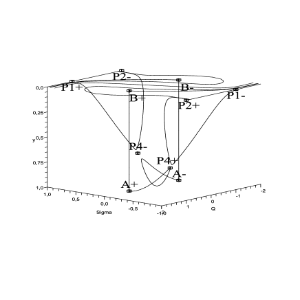
Figure 1: Projection of the phase space on the invariant set $x=0$, in the case of radiation ($w=1/3,n=2$). There is one orbit of type ${\cal B}_{+}\longrightarrow{\cal A}_{+}$ and one of type ${\cal A}_{-}\longrightarrow{\cal B}_{-}$. The existence of an heteroclinic sequence of type ${\cal A}_{-}\longrightarrow P_{4}^{-}\longrightarrow P_{4}^{+}\longrightarrow{\cal A}_{+}$ corresponds to a cosmological bounce.

Similarly to the isotropic case (see figure 5 of [11]) there is one orbit of type ${\cal B}_{+}\longrightarrow{\cal A}_{+}$ and one of type ${\cal A}_{-}\longrightarrow{\cal B}_{-}$. However, in the present case we have the additional existence of an heteroclinic sequence of type ${\cal A}_{-}\longrightarrow P_{4}^{-}\longrightarrow P_{4}^{+}\longrightarrow{\cal A}_{+}$, corresponding to the transition from collapsing AdS to expanding dS phase, that is we obtain a cosmological bounce followed by a de Sitter expansion, which could describe the inflationary stage. This significant behavior is a pure result of the anisotropy and reveals the capabilities of the scenario. Lastly, note the very interesting possibility, of the eternal transition $P_{1}^{-}\longrightarrow P_{2}^{+}\longrightarrow P_{1}^{-}\longrightarrow P_{2}^{+}\cdots$ which is just the realization of cyclic cosmology [26]. Bouncing solutions are found to exist both in FRW $R^{n}$-gravity [27], as well as in the Bianchi I and Bianchi III $R^{n}$-gravity [14] (see also [28]), and thus they arise from the $R^{n}$ gravitational sector.

4 Conclusions

As we saw, the universe at late times can result to a state of accelerating expansion, and additionally, for a particular $n$-range ($2<n<3$) it exhibits phantom behavior. Additionally, the universe has been isotropized, independently of the anisotropy degree of the initial conditions, and it asymptotically becomes flat. The fact that such features are in agreement with observations [1] is a significant advantage of the model. Moreover, in the case of radiation ($n=2$, $w=1/3$) the aforementioned stable solution corresponds to a de-Sitter expansion, and it can also describe the inflationary epoch of the universe. In our work we extracted our results without relying at all on the cosmic no-hair theorem, which is a significant advantage of the analysis [25].

The Kantowski-Sachs anisotropic $R^{n}$-gravity can also lead to contracting solutions, either accelerating or decelerating, which are not globally stable. Thus, the universe can remain near these states for a long time, before the dynamics remove it towards the above expanding, accelerating, late-time attractors. The duration of these transient phases depends on the specific initial conditions.

One of the most interesting behaviors is the possibility of the realization of the transition between expanding and contracting solutions during the evolution. That is, the scenario at hand can exhibit the cosmological bounce or turnaround. Additionally, there can also appear an eternal transition between expanding and contracting phases, that is we can obtain cyclic cosmology. These features can be of great significance for cosmology, since they are desirable in order for a model to be free of past or future singularities.

References

- [1] M. Kowalski et al., Astrophys. J. 686, (2008) 749; S. W. Allen, D. A. Rapetti, R. W. Schmidt, H. Ebeling, G. Morris and A. C. Fabian, Mon. Not. Roy. Astron. Soc. 383, (2008) 879; K. N. Abazajian et al., Astrophys. J. Suppl. 182, (2009) 543; N. Jarosik et al., Astrophys. J. Suppl. 192 (2011) 14.
- [2] T. P. Sotiriou and V. Faraoni, Rev. Mod. Phys. 82, (2010) 451; A. De Felice and S. Tsujikawa, Living Rev. Rel. 13, (2010) 3.
- [3] C. W. Misner, K. S. Thorne and J. A. Wheeler, Gravitation, San Francisco, W. H. Freeman & Co. (1973); P. J. E. Peebles, Principles of physical cosmology, Princeton, USA: Univ. Pr. (1993) 718 p.;
- [4] G. F. R. Ellis and M. A. H. MacCallum, Commun. Math. Phys. 12, (1969) 108; C. G. Tsagas, A. Challinor and R. Maartens, Phys. Rept. 465, (2008) 61.
- [5] A.S. Kompaneets and A.S. Chernov, Zh. Eksp. Teor. Fiz. 47, (1964) 1939. English translation: Soviet. Phys. JETP 20, (1965) 1303; R. Kantowski and R. K. Sachs, J. Math. Phys. 7 443 (1966); C. B. Collins, J. Math. Phys. 18 (1977) 2116; E. Weber, J. Math. Phys. 25, (1984) 3279; O. Gron, J. Math. Phys. 27, (1986) 1490; M. Demianski, Z. A. Golda, M. Heller and M. Szydlowski, Class. Quant. Grav. 5, (1988) 733; L. Bombelli and R. J. Torrence, Class. Quant. Grav. 7, (1990) 1747; L. M. Campbell and L. J. Garay, Phys. Lett. B 254, (1991) 49; L. E. Mendes and A. B. Henriques, Phys. Lett. B 254, (1991) 44; P. Vargas Moniz, Phys. Rev. D 47, (1993) 4315; M. Cavaglia, Mod. Phys. Lett. A 9, (1994) 1897; S. Nojiri, O. Obregon, S. D. Odintsov and K. E. Osetrin, Phys. Rev. D 60, (1999) 024008; A. K. Sanyal, Phys. Lett. B 524, (2002) 177; X. Z. Li and J. G. Hao, Phys. Rev. D 68, (2003) 083512; W. F. Kao, Phys. Rev. D 74, (2006) 043522.
- [6] G. Leon, E. N. Saridakis, Class. Quant. Grav. 28, (2011) 065008.
- [7] A. S. Eddington, Mon. Not. Roy. Astron. Soc. 90, (1930) 668.
- [8] E. R. Harrison, Rev. Mod. Phys. 39, (1967) 862; G. W. Gibbons, Nucl. Phys. B292, (1987) 784 ; J. D. Barrow, G. F. R. Ellis, R. Maartens and C. Tsagas Class. Quant. Grav. 20, (2003) L155.
- [9] S. Byland and D. Scialom, Phys. Rev. D 57, (1998) 6065; U. Camci, I. Yavuz, H. Baysal, I. Tarhan and I. Yilmaz, Int. J. Mod. Phys. D 10,(2001) 751; A. A. Coley, W. C. Lim and G. Leon, arXiv:0803.0905 [gr-qc].
- [10] R. Goswami, N. Goheer and P. K. S. Dunsby, Phys. Rev. D 78, (2008) 044011.
- [11] N. Goheer, R. Goswami and P. K. S. Dunsby, Class. Quant. Grav. 26, (2009) 105003.
- [12] G. F. R. Ellis, Cargèse Lectures in Physics, Vol 6 (ed) E Scatzman (New York: Gordon and Breach) (1973); G. F. R. Ellis and H. van Elst, Cosmological Models (Cargèse Lectures 1998), Theoretical and Observational Cosmology (ed) M. Lachièze-Rey (Kluwer, Dordrecht) (1999) 1-116; H. van Elst and C. Uggla, Class. Quant. Grav. 14, (1997) 2673.
- [13] S. Carloni, P. K. S. Dunsby, S. Capozziello and A. Troisi, Class. Quant. Grav. 22, (2005) 4839.
- [14] N. Goheer, J. A. Leach and P. K. S. Dunsby, Class. Quant. Grav. 24, (2007) 5689.
- [15] S. Capozziello, Int. J. Mod. Phys. D 11, (2002) 483; S. Capozziello, S. Carloni and A. Troisi, Recent Res. Dev. Astron. Astrophys. 1, (2003) 625.
- [16] S. Capozziello, M. De Laurentis and V. Faraoni, arXiv:0909.4672 [gr-qc].
- [17] C. B. Collins Commun. Math. Phys. 23 (1971) 137; C. B. Collins and S. W. Hawking, Astrophys. J., Vol. 180, (1973) 317.
- [18] J. Wainwright and W. C. Lim, J. Hyperbol. Diff. Equat. 2 (2005) 437.
- [19] J. A. Leach, S. Carloni and P. K. S. Dunsby, Class. Quant. Grav. 23, (2006) 4915.
- [20] H. Poincaré J. Mathématiques 7 (1881) 375; L. Perko, Differential equations and dynamical systems, New York: Springer Verlag (1996).
- [21] M. Goliath and G. F. R. Ellis, Phys. Rev. D. 60, (1999) 023502.
- [22] N. Goheer, J. A. Leach and P. K. S. Dunsby, Class. Quant. Grav. 25, (2008) 035013.
- [23] D. M. Solomons, P. Dunsby and G. Ellis, Class. Quant. Grav. 23, (2006) 6585.
- [24] S. Wiggins, Introduction to Applied Nonlinear Dynamical Systems and Chaos, Springer (2003).
- [25] R. M. Wald, Phys. Rev. D 28, (1983) 2118.
- [26] P. J. Steinhardt and N. Turok, Phys. Rev. D 65, (2002) 126003; S. Mukherji and M. Peloso, Phys. Lett. B 547, (2002) 297; J. Khoury, P. J. Steinhardt and N. Turok, Phys. Rev. Lett. 92, (2004) 031302; L. Baum and P. H. Frampton, Phys. Rev. Lett. 98, (2007) 071301; E. N. Saridakis, Nucl. Phys. B 808, 224 (2009); Y. F. Cai and E. N. Saridakis, Class.Quant.Grav. 28 (2011) 035010.
- [27] S. Carloni, P. K. S. Dunsby and D. M. Solomons, Class. Quant. Grav. 23, 1913 (2006).
- [28] C. Barragan and G. J. Olmo, Phys. Rev. D 82, 084015 (2010).