Computing the demagnetizing tensor for finite difference micromagnetic simulations via numerical integration

Abstract

In the finite difference method which is commonly used in computational micromagnetics, the demagnetizing field is usually computed as a convolution of the magnetization vector field with the demagnetizing tensor that describes the magnetostatic field of a cuboidal cell with constant magnetization. An analytical expression for the demagnetizing tensor is available, however at distances far from the cuboidal cell, the numerical evaluation of the analytical expression can be very inaccurate.

Due to this large-distance inaccuracy numerical packages such as OOMMF compute the demagnetizing tensor using the explicit formula at distances close to the originating cell, but at distances far from the originating cell a formula based on an asymptotic expansion has to be used. In this work, we describe a method to calculate the demagnetizing field by numerical evaluation of the multidimensional integral in the demagnetizing tensor terms using a sparse grid integration scheme. This method improves the accuracy of computation at intermediate distances from the origin.

We compute and report the accuracy of (i) the numerical evaluation of the exact tensor expression which is best for short distances, (ii) the asymptotic expansion best suited for large distances, and (iii) the new method based on numerical integration, which is superior to methods (i) and (ii) for intermediate distances. For all three methods, we show the measurements of accuracy and execution time as a function of distance, for calculations using single precision (4-byte) and double precision (8-byte) floating point arithmetic. We make recommendations for the choice of scheme order and integrating coefficients for the numerical integration method (iii).

I Introduction

Micromagnetic simulation of ferromagnetic nanostructures is a widespread tool to support research and device design in a variety of fields, including magnetic data storage and sensing. The micromagnetic theory is based on partial differential equations proposed in Brown1963a combined with an equation of motion that can be solved to determine the time-development of the magnetization vector function.

I.1 Micromagnetics

Numerical simulations in micromagnetics commonly solve the Landau-Lifshitz-Gilbert and the associated partial differential equations using a finite difference discretization of space (including OOMMF, LLG Micromagnetics Simulator, Micromagus, Mumax, Micromagnum oommf ; llg ; micromagus ; mumax ; micromagnum ). In the finite difference method, space is discretized using a regular grid with cuboidal cells, and the magnetization and other scalar and vector fields involved in the computation are assumed to be constant within each of these cubiodal cells. The magnetization vector field $\mathbf{M}$ is the primary degree of freedom. As a function of $\mathbf{M}$, which is represented by a constant within every cell, various fields such as the exchange, anisotropy, Zeeman, and demagnetizing fields are computed. These are added together, and enter the equation of motion for $\mathbf{M}$ as the effective field.

The most demanding part of the calculation is to determine the demagnetizing field: to compute the demagnetizing field for one of the discretization cells, an integral over the whole magnetic domain has to be carried out, which translates into a (triple) sum (in a 3d system) over all cells in the finite difference discretization.

For a finite difference discretization of a three-dimensional sample with $n_{1}$ discretization points in the x-direction, $n_{2}$ points in the y-direction and $n_{3}$ points in the z-direction, there are $n=n_{1}n_{2}n_{3}$ cuboidal cells in total. To compute the demagnetizing field in each one of these cells, we need to consider the total contribution of all $n$ cells. Thus, to work out the demagnetizing field for all $n$ cells requires $\mathcal{O}(n^{2})$ operations using a naive approach. For realistic mesh sizes this is infeasible. Instead, usually the demagnetizing field $\mathbf{H}$ is expressed as a discrete convolution of the so-called demagnetizing tensor $\mathbf{N}$ and the representation of the magnetization $\mathbf{M}$

$$\mathbf{H}_{i_{1}i_{2}i_{3}}=-\sum_{j_{1}=1}^{n_{1}}\sum_{j_{2}=1}^{n_{2}}\sum_{j_{3}=1}^{n_{3}}\mathbf{N}(\mathbf{r}_{i_{1}i_{2}i_{3}}-\mathbf{r}_{j_{1}j_{2}j_{3}})\cdot\mathbf{M}_{j_{1}j_{2}j_{3}},$$ (1)

The triple indices $i_{1}i_{2}i_{3}$ are used to index cells in the 3d-discretization, i.e. $i_{1}$ counting cells in the x-direction, and correspondingly $i_{2}$ and $i_{3}$ in y- and z- direction. The vector $\mathbf{r}_{i_{1}i_{2}i_{3}}$ points to the centre of the cell $i_{1}i_{2}i_{3}$ and $\mathbf{M}_{i_{1}i_{2}i_{3}}$ is the magnetization in that cell, and $\mathbf{H}_{i_{1}i_{2}i_{3}}$ is the demagnetizing field in that cell.

The discrete convolution (1) is typically carried out as a product in Fourier space as the regular spacing of the finite difference cells allows straightforward use of the Fast Fourier Transform and its inverse. The demagnetizing tensor $\mathbf{N}$ needs to be computed once for given geometry and discretization, normally at the setup stage of the simulation. In this work we propose a new procedure for the accurate computation of entries in the demagnetizing tensor.

The tensor $\mathbf{N}(\mathbf{r})$ describes the energy of the demagnetizing interaction between two uniformly magnetized cuboids $\sigma_{1}$ and $\sigma_{2}$ of volume $|\sigma|$ separated by the translation vector $\mathbf{r}$. It is a symmetric tensor of rank 2, which we write in the dimensionless form following the convention from Newell1993

$$\mathbf{N}(\mathbf{r}) =-\frac{1}{4\pi|\sigma|}\int_{\sigma_{1}}\mathrm{d}{\mathbf{r}_{1}}\int_{\sigma_{2}(\mathbf{r})}\nabla_{{\mathbf{r}}_{1}}\nabla_{\mathbf{r}_{2}}\frac{1}{|\mathbf{r}_{1}-\mathbf{r}_{2}|}\,\mathrm{d}\mathbf{r}_{2}$$ (2)

$$E_{\sigma_{1}\leftrightarrow\sigma_{2}} =\mu_{0}|\sigma|\,\mathbf{M}_{1}\cdot\mathbf{N}(\mathbf{r})\cdot\mathbf{M}_{2}$$ (3)

The computation of the demagnetizing field using the formula (1) follows the commonly used energy-based approach to the discretization of the Landau-Lifshitz-Gilbert equation Miltat2007 . In this approach (used in OOMMF oommf and in our work), the components of the effective field in each cuboidal cell are obtained via a minimization procedure applied to the discretized total energy $E_{\mathrm{total}}=\sum_{\sigma_{1},\sigma_{2}}E_{\sigma_{1}\leftrightarrow\sigma_{2}}$. In contrast, in the field-based approach the discretized fields are obtained from the corresponding continuous fields by e.g. sampling at the cell center Labrune1995 ; Albuquerque2002 ; Toussaint2002 ; Miltat2007 , and the demagnetizing tensor (2) is not used.

I.2 Numerical accuracy of $\mathbf{N}(\mathbf{r})$ evaluation

The components of the demagnetizing tensor can be computed via an analytical formula Schabes1987 ; Newell1993 ; maicus1998magnetostatic ; fukushima1998volume . However, when $\mathbf{r}=\mathbf{r}_{a}-\mathbf{r}_{b}$ is large compared to the size of the mesh cells (i.e. when the interacting mesh cells at $\mathbf{r}_{a}$ and $\mathbf{r}_{b}$ are far apart on the grid), evaluation of this expression on a computer can result in a loss of significant digits, to a point where the computed answer contains no significant digits at all Donahue2007 .

The loss of accuracy is caused by catastrophic cancellation: the terms of the analytical expression correspond to indefinite integrals with $r^{3}$ order of growth, while the demagnetizing tensor itself (the definite integral) is of the order $1/r^{3}$. On modern CPUs, double-precision floating numbers contain approximately 15 significant digits, therefore the relative error in the computation of the demagnetizing tensor using the analytical formula is of the order $10^{-15}r^{6}$. One can therefore expect that for cell separations greater than $10^{15/6}\approx 300$ the analytical computation will contain no significant digits at all (i.e., the relative error will be greater than 1).

Indeed, the above estimate is confirmed if the result of the computation using the analytical formula is compared to the exact (up to machine precision) value of the demagnetizing tensor. The exact value is computed using specialized high-precision libraries (see Sec. II.2 and III.7). As seen in Fig. 1, the relative error $\eta$ of the analytical computation grows as $r^{6}$ and crosses the $\eta=1$ threshold at a separation of about 300 cells.

The micromagnetic simulation package OOMMF counteracts this inaccuracy problem by utilizing an asymptotic expansion of the demagnetizing tensor Donahue2007 in terms of powers of $1/r$ up to 6th order. In this paper we investigate an alternative approach to deal with the catastrophic cancellation problem, which is to compute the integral (2) directly using numerical integration.

II Method

As outlined in section I, the 6-d integral described in (2) can be computed using

• an analytical formula Newell1993 ,

• an asymptotic expansion Donahue2007 ,

• numerical integration.

For computing integrals in one dimension, multiple highly-accurate methods are available. However, the computation of multidimensional integrals is hindered by the so-called curse of dimensionality, where the number of integration points increases exponentially with the increase in dimension. Since the demagnetizing tensor $\mathbf{N}(\mathbf{r})$ has to be computed for all possible grid offsets $\mathbf{r}$, the integration method for this six-dimensional integral needs to be both accurate and fast.

The tradeoff between accuracy and computational effort can be achieved using the sparse grid family of methods, also known as Smolyak quadrature Smolyak1963 (for a brief review of other alternatives see Petras2003 ).

The sparse grid method is used to extend one-dimensional integration rules to integration formulas in multiple dimensions. Below we summarize the key ideas of the method Petras2003 . Starting with a one-dimension family of integration formulas $I_{k}$ for computing the 1d integral

$$\int_{0}^{1}f(x)dx\approx I_{k}[f]=\sum_{i=1}^{n_{k}}a_{ki}f(x_{ki})$$ (4)

we can write the formal identity

$$\int_{0}^{1}f(x)dx =I_{0}[f]+(I_{1}[f]-I_{0}[f])+\ldots$$

$$=\Delta_{0}[f]+\Delta_{1}[f]+\ldots$$

where $\Delta_{k}=I_{k}-I_{k-1}$ and $\Delta_{0}=I_{0}$.

An example for a family of integration formulas $I_{k}$ are Gaussian integration formulae with $k+1$ points.

Now, we apply the above formal identity $d$ times to obtain a $d$-dimensional integration rule

$$\int_{[0,1]^{d}}f(\mathbf{x})d\mathbf{x}=\Big{(}\prod_{j=1}^{d}(\Delta_{0}^{(j)}+\Delta_{1}^{(j)}+\ldots)\Big{)}[f]$$ (5)

Here the $\Delta_{k}^{(j)}$ operator applies the approximation (4) to the $j$-th argument of the function $f$, and the $\prod$ symbol represents the operator product, i.e. repeated application of $\sum_{k}\Delta_{k}^{(j)}$ in all $d$ dimensions.

The formal expansion (5) is infinite; to obtain a practical integration formula we need to truncate it. Smolyak quadrature achieves this by expanding the product (5) and grouping together terms $\Delta_{i_{1}}^{(1)}\cdots\Delta_{i_{d}}^{(d)}$ with the same term order $k=i_{1}+\ldots+i_{d}$:

$$\int_{[0,1]^{d}}f(\mathbf{x})d\mathbf{x} =Q_{0}[f]+Q_{1}[f]+\ldots$$ (6)

$$\approx Q_{0}[f]+Q_{1}[f]+\ldots+Q_{k}[f]$$ (7)

where

$$Q_{k}[f]=\sum_{i_{1}+\ldots+i_{d}=k}\Delta_{i_{1}}^{(1)}\Delta_{i_{2}}^{(2)}\cdots\Delta_{i_{d}}^{(d)}[f]$$ (8)

Compared to the evaluation of the $d$-dimensional integral using a naive $d$-fold product (which required $n_{k}^{d}$ integration points for rule $I_{k}$), the Smolyak formula (7) greatly reduces the number of integration points required to achieve a certain level of accuracy, as long as the integrand is reasonably smooth.

Different one-dimensional families (4) will result in different multidimensional formulas (7); in our testing for the demagnetizing integrand (2) we obtained the best results when using the “delayed Kronrod-Patterson sequence” developed by Petras Petras2003 . The delayed sequence is based on the Kronrod-Patterson family of 1d integration formulas $I_{k}^{\mathrm{KP}}$ Patterson1968 , however some of the formulas are repeated to lower the rank of approximation (and the required number of integration points), determined by the “delay sequence“ $k_{i}$:

$$I_{i}^{\mathrm{delayed}}=I_{k_{i}}^{\mathrm{KP}}$$ (9)

For the maximum delay sequence Petras2003 the formulas are repeated so that the 1-d rule $I_{i}^{\mathrm{delayed}}$ is accurate for polynomials up to rank $i$:

$$k_{i}^{\mathrm{full}}=0,1,1,2,2,2,3,3,3,3,3,3,4,\ldots$$ (10)

II.1 Integrand

II.1.1 6d method

A straightforward way to compute the demagnetizing tensor numerically would be to apply the sparse grid formulas to the 6-d integral (2).

II.1.2 4d method

Due to the high dimensionality of the 6d integral, the number of required integration points will be quite high. To reduce the dimensionality, we can transform the 6-d volume integral $\eqref{eq-n}$ to a 4-d surface integral using a variant of Gauss’s theorem. The procedure is described in Newell1993 and results in the following formulas for the components of the demagnetizing tensor where we have used the notation of Newell1993

$$N_{xx}(X,Y,Z)=\frac{1}{4\pi\Delta x\,\Delta y\,\Delta z}\big{[}2F(X,Y,Z)-F(X+\Delta x,Y,Z)-F(X-\Delta x,Y,Z)\big{]}$$

$$N_{xy}(X,Y,Z)=\frac{1}{4\pi\Delta x\,\Delta y\,\Delta z}\big{[}G(X,Y,Z)-G(X-\Delta x,Y,Z)-G(X,Y+\Delta y,Z)+G(X-\Delta x,Y+\Delta y,Z)\big{]}$$

with

$$F(X,Y,Z)=\int\limits_{0}^{\Delta z}\int\limits_{0}^{\Delta y}\int\limits_{0}^{\Delta z}\int\limits_{0}^{\Delta y}\frac{dz\,dy\,dz^{\prime}\,dy^{\prime}}{\sqrt{X^{2}+(y+Y-y^{\prime})^{2}+(z+Z-z^{\prime})^{2}}}$$

and

$$G(X,Y,Z)=\int\limits_{Y-\Delta y}^{Y}\int\limits_{Z-\Delta z}^{Z}\int\limits_{z}^{z+\Delta z}\int\limits_{X}^{X+\Delta x}\frac{dy\,dz\,dz^{\prime}\,dx^{\prime}}{\sqrt{x^{\prime 2}+y^{2}+z^{\prime 2}}}$$

where $(X,Y,Z)=\mathbf{r}$ is the vector between the two interacting cells, and $\Delta x$, $\Delta y$, $\Delta z$ are the edge lengths of the cuboidal cells.

To simplify the application of numerical integration formulas, we transform the above expressions so that integration is performed over the unit cube $[0,1]^{4}$.

$$N_{xx}(X,Y,Z)=\int\limits_{0}^{1}\int\limits_{0}^{1}\int\limits_{0}^{1}\int\limits_{0}^{1}\big{[}2\mathcal{F}(X,Y,Z)-\mathcal{F}(X+\Delta x,Y,Z)-\mathcal{F}(X-\Delta x,Y,Z)\big{]}\,dz\,dy\,dz^{\prime}\,dy^{\prime}$$ (11)

$$N_{xy}(X,Y,Z)=\int\limits_{0}^{1}\int\limits_{0}^{1}\int\limits_{0}^{1}\int\limits_{0}^{1}dy\,dz\,dz^{\prime}\,dx^{\prime}\times\\ \times\big{[}\mathcal{G}(X,Y,Z)-\mathcal{G}(X-\Delta x,Y,Z)-\mathcal{G}(X,Y+\Delta y,Z)+\mathcal{G}(X-\Delta x,Y+\Delta y,Z)\big{]}$$ (12)

with

$$\mathcal{F}(X,Y,Z)=\frac{\Delta y\,\Delta z}{4\pi\,\Delta x}\frac{1}{\sqrt{X^{2}+(\Delta y\,y+Y-\Delta y\,y^{\prime})^{2}+(\Delta z\,z+Z-\Delta z\,z^{\prime})^{2}}}$$

$$\mathcal{G}(X,Y,Z)=\frac{\Delta z}{4\pi}\frac{1}{\sqrt{(X+\Delta x\,x^{\prime})^{2}+(Y+\Delta y(y-1))^{2}+(Z+\Delta z(z+z^{\prime}-1))^{2}}}$$

The remaining components of the tensor can be obtained by variable substitution (for example, $N_{yz}(X,Y,Z)=N_{xy}(Y,Z,X)$).

In this approach, we are essentially computing two dimensions of the 6-d integral analytically, and the remaining four numerically. As we shall see, the two analytical steps introduce a small amount of cancellation, but the required number of integration points is significantly reduced.

II.2 Error estimation

To determine the accuracy of the computed demagnetizing tensor $\mathbf{N}$, we compute its exact (to machine precision) value $\mathbf{N}_{\text{exact}}$ via the analytical formula using the GNU MPFR high-precision floating point library Fousse2007 , and evaluate the relative error $\eta$:

$$\eta=\frac{||\mathbf{N}-\mathbf{N}_{\text{exact}}||}{||\mathbf{N}_{\text{exact}}||}$$ (13)

where the matrix norm is defined as $||\mathbf{N}||=\sqrt{\sum_{i,j}N_{ij}^{2}}$.

III Results

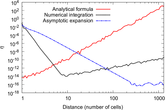
Figure 1: The relative error $\eta$ in the computation of the demagnetizing tensor as a function of the distance between the interacting cuboids, $1\!\times\!1\!\times\!1$ cell size, Kronrod-Patterson sparse grid integration with full delay, order $k=7$ Petras2003 , double precision arithmetic (precision $\sim 10^{-16}$).

III.1 Overview

Figure 1 shows the comparison of the accuracy of the analytical formula, the asymptotic expansion, and the numerical sparse grid integration methods as a function of the distance between cells using (8 byte) double floating point. For the numerical sparse grid integration, the 4d method (Sec. II.1.2) has been used.

While the aspect ratio of the cuboidal cell with edge lengths $\Delta x,\Delta y$ and $\Delta z$ affects the results somewhat, they are independent of the absolute size of the cuboidal cell. We have chosen $\Delta x,\Delta y$ and $\Delta z=(1,1,1)$ so that the distance $|\mathbf{r}|$ between interacting cuboids is expressed in the number of cells between the interacting cuboids. For example, for a micromagnetic simulation with a $5\,\mathrm{nm}\times 5\,\mathrm{nm}\times 5\,\mathrm{nm}$ cell size, the distance of 10 on the plot in Figure 1 corresponds to a $50\,\mathrm{nm}$ distance on the mesh.

We start by discussing the analytical formula shown as a red solid line in Fig. 1. Its relative error $\eta$ for very short distances is $10^{-14}$. We cannot expect an error below $10^{-16}$ as this is the precision of the double floating point numbers used. As the distance between interacting cells increases, the analytical formula becomes less accurate. At a separation of 100 cells, it is about $10^{-4}$, meaning that only the first 4 digits are correct. In fact, beyond a distance of about 300 cells the relative error becomes greater than 1, indicating that no digits of the double float can be expected to be correct and that not considering the demagnetizing tensor beyond that point would be more accurate than computing it analytically.

The asymptotic expansion (blue dash-dotted line in Fig. 1) starts with a large relative error $\eta\sim 10^{-2}$ for short distances, which decreases as the distance increases. At about 200 cells distance, the relative error is $\sim 10^{-15}$ and remains of that magnitude for larger distances. The smooth reduction of the error with distance reflects the way the high-order moments of the cuboid interaction decay with increasing distance, thus making the asymptotic approximation increasingly more accurate. The asymptotic expansion is more accurate than the exact analytical expression for distances greater than about 11 cells.

The precise number of cells for which this crossover occurs depends on the aspect ratio of the discretization cell as well as the direction of the separation vector between the two interacting cuboids. In practical implementations of finite difference micromagnetic codes a crossover point needs to be identified. In OOMMF, by default the asympotic formula is used for distances above 32 cells, which for this example corresponds to an error of $10^{-6}$.

The numerical sparse grid integration error (black dotted line in Fig. 1) also starts around $10^{-2}$ for short distances and decays to $~{}10^{-14}$ for a cell distance of about 7. For very short distances, the integrand (2) varies quickly (it diverges for $|\mathbf{r}|\rightarrow 0$) and numerical integration is inaccurate. For cell distances between 7 and 70, numerical integration is more accurate than the analytical expression, and more accurate than the asymptotic expansion. Beyond radius 70, the asymptotic expansion is more accurate than numerical integration. The slight inrease in the relative error of the numerical formula with increasing distance is caused by the cancellation introduced by Gauss’s theorem (see II.1.2).

In summary, the numerical evaluation of the analytical formula is most accurate for short distances, and the asymptotic expansion is most accurate for long distances. The new sparse grid integration method introduced here is most accurate for intermediate distances.

III.2 Sparse grid integration parameters and execution performance

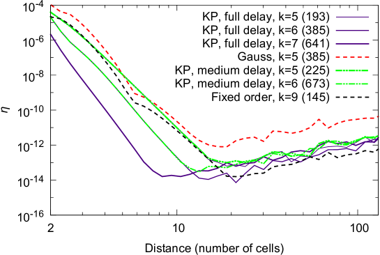
Figure 2: Comparison of numerical integration schemes for computing the 4d integral (11)-(12); KP: sparse grid integration based on the delayed Kronrod-Patterson 1d rule Petras2003 ; Gauss: sparse grid integration based on the delayed Gauss 1d rule; fixed order: 9th order rule with 145 integration points ecf ; Sorevik85 ; $k$: the rule’s order of approximation; ($\cdot$): the number of integration points.

In the sparse grid method, the order of approximation is a parameter that can be adjusted to reach the desired level of accuracy or performance. For lower orders of approximation, one can also use fixed-order integration formulas that usually provide the same accuracy with fewer integration points. An extensive library of such formulas is available ecf ; Cools2003 ; Cools1999 ; Cools1993 .

Since the computation of the demagnetizing tensor is a one-off cost, higher order, more accurate integration formulas would be preferable. In Figure 2 we show the results for a number of sparse grid formulas as well as for a 145-point fixed-order formula from ecf ; Sorevik85 .

The most accurate method considered here is the 641-point 7th order sparse grid method based on the 1d Kronron-Patterson sequence with full delay Petras2003 . The delayed Kronrod-Patterson methods with orders 6 and 5 have fewer points and decreased accuracy. Formulas based on Gauss or Kronrod-Patterson sequences with medium delay require extra integration points to achieve the same level of accuracy and are thus suboptimal compared to the Kronrod-Patterson family with full delay.

The 145-point fixed order formula is more accurate than the 193-point 5th order Kronrod-Patterson formula, but slightly less accurate than the 385-point 6th order formula.

Based on these results, we recommend using either the 145-point fixed order formula or the Kronrod-Patterson fully delayed formula with order 6 or 7, depending on required accuracy and performance.

III.3 Comparison of 4d and 6d integration

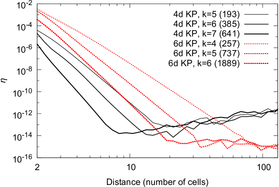
Figure 3: Comparison of numerical integration of the 4d integral (11)-(12) versus the 6d integral (2), Kronrod-Patterson 1d rule with full delay, $1\!\times\!1\!\times\!1$ cells.

As an alternative to computing the 4d integral (method II.1.2), we can also compute all of the 6 integrations numerically (method II.1.1). The results for the 6d integration method are shown in Figure 3. All red dashed curves show results for the 6d method, and all black solid lines show results for the 4d method.

Both for the three 4d data sets and the three 6d data sets, we can see that the decrease in the error with increasing distance is faster for higher order methods. The 4d lines show minimal error between 8 and 11 cells distance, and for larger distances the error increases a little — this reflects the numerical cancellation from subtracting large terms that increase with distance and originate from the analytical integration that has been carried out over 2 dimensions. On the contrary, the 6d data sets — where the whole 6d integral has been computed numerically — does not suffer from this and the error remains small ($<10^{-14}$) for larger distances. However, the number of evaluation points is higher compared to the 4d method.

As seen in Figure 2, even the lowest order quadrature formula gives a sufficient accuracy gain in the intermediate range to be better than the analytic and the asymptotic expression. However, in time-dependent micromagnetic simulations the computation of the demagnetizing tensor is a one-time setup cost, and the setup cost is only slightly influenced by the order of the integration formula — one might as well choose the higher order, more accurate formula.

Comparing the 4d and 6d method, we suggest the 4d method as it is faster to compute. The 4d method is less accurate than the 6d for the largest distances but this is of little practical concern — for those distances, the asymptotic expansion can be used instead.

III.4 Performance

In table 1, we show performance measurements for computing the entries in the demagnetizing tensor. For the fixed order (k=9) 145-point integration rule, the computational cost is comparable to the analytical formula, while the KP full delay (k=7) 641-point rule is approximately 5 times slower. The total cost of evaluating the demagnetizing tensor on a $400\times 40\times 1$ mesh was $95\,\mathrm{ms}$ (Table 2) for the 145-point rule and $351\,\mathrm{ms}$ for the 641-point rule. Since a typical dynamical micromagnetic simulation usually requires 10,000 or more time steps, the one-time cost of setting up the demagnetizing tensor is minor even for the 641-point rule. For the sample system studied here, evaluating the effective field and dm/dt once takes $4\,\mathrm{ms}$. We also note that as the mesh grows larger, more of the entries can be computed using the extremely fast asymptotic formula, resulting in sublinear scaling of the total cost with mesh size $n$.

Method	Time per cell, ns
Analytical	8.5
Integration, 145 points	9.8
Integration, 641 points	43.2
Asymptotic	0.2

Table 1: Per-cell cost of computing the entries of the demagnetizing tensor, workstation: dual CPU Intel E5506 2.13 GHz (8 threads), compiler: GCC 4.7.2.

Method	Total time, ms
Combined, 145 points	95
Combined, 641 points	351
LLG dm/dt evaluation	4

Table 2: Total cost of computing the demagnetizing tensor for a $2000\times 200\times 20\,\mathrm{nm}^{3}$ mesh, $5\times 5\times 20\,\mathrm{nm}$ cells.

III.5 Single point floating precision

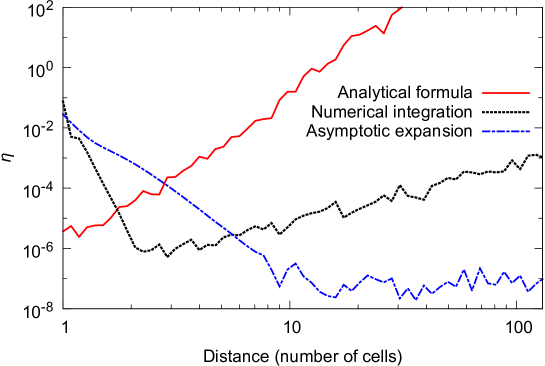
Figure 4: The relative error $\eta$ of computing the demagnetizing tensor using single precision arithmetic (precision $\sim 10^{-7}$), $1\!\times\!1\!\times\!1$ cell size, Kronrod-Patterson sparse grid integration with full delay, order $k=7$.

The recent rise of General Purpose computing on Graphical Processing Units (GPGPU) has re-invigorated single-precision floating point operations: on these architectures single precision floating point operations are generally much faster, and on cheaper cards the only type of floating point operations provided. Additionally, the available RAM on the GPU card is limited, providing another incentive to use single rather than double precision floating point numbers.

We repeat the study presented in figure 1 but use single precision numbers for all methods and show the results in figure 4. The qualitative findings are the same as for double precision numbers: the most accurate methods are as a function of increasing distance: (i) the analytical formula, (ii) the sparse grid numerical integration technique and (iii) the asymptotic expression.

However, the relevant cross-over points have moved to shorter distances. The analytical expression becomes less accurate than numerical integration for more than 2 cells distance, and the asymptotic expression is more accurate than numerical integration for spacings greater than 8 cells.

As mentioned in III.1 we find that the analytical expression for double precision (Figure 1) provides only 4 significant digits (i.e. a relative error of $10^{-4}$) for a distance of 100 cells. For single precision (Figure 4) we find that the analytical expression provides the same level of accuracy (i.e. 4 significant digits) only for distances up to 3 cells. Correspondingly, the distance for which the relative error exceeds 1, moves from over 300 cells with double precision to 11 cells with single precision.

The accurate calculation of the demagnetizing tensor entries using single precision floating point numbers only is challenging – using the best methods currently known and combining the three methods shown in figure 4, the relative error can be kept around or below $10^{-4}$.

For practical use of GPGPU single precision calculations for micromagnetic simulation, we recommend to compute the demagnetizing tensor using double-precision – either on the GPU with some reduction in speed if the GPU hardware supports this, or on the CPU with a more significant time penalty. As the computation of the demagnetizing tensor (2) only needs to be done once and subsequent computations of the demagnetizing field as required for energy minimisation or time stepping only require to carry out the convolution (1), it should be acceptable to increase the accuracy of the demagnetizing tensor for a one-off time penalty in the setup phase.

III.6 Forward and backward Fast Fourier Transform

Our tests showed that the forward and inverse fast Fourier transforms required to compute the convolution (1) did not introduce any significant numerical error in the calculation of the demagnetizing field (either single or double precision).

III.7 Other high accuracy methods

We note for completeness that there are other options to compute the demagnetizing tensor more accurately than any of the methods outlined above if high accuracy is of utmost importance.

There are high precision arithmetic libraries available which provide software implementations of floating point operations: the library user can choose the number of significant digits used in the calculations (where 8 would approximately correspond to single precision accuracy and 16 to double precision floating point numbers). The larger the number of significant digits to be used, the slower is the execution of these operations. We have used this technique to obtain the reference data $\mathbf{N}_{\text{exact}}$ required to compute the error $\eta$ (13). Using such libraries requires significant changes to source code, and execution is extremely slow. It is impractical to use such libraries for micromagnetic simulation.

IV Summary

We have compared the accuracy of computing the demagnetizing tensor using the analytical formula, the asymptotic expansion, and numerical integration. We obtain and provide quantitative data on the relative error of demagnetizing tensor entries computed using all three methods.

We propose a new method using numerical integration to compute the entries of the demagnetizing tensor which allows to increase the accuracy from an error of $10^{-8}$ to an error of only $10^{-12}$ for intermediate distances of between 4 and 80 simulation cells for the commonly used double precision floating point numbers. In the context of micromagnetic simulations, we find that the 7th order 641-point Kronrod-Patterson sparse grid formula with full delay Petras2003 and the fixed-order 145-point rule ecf ; Sorevik85 provide a reasonable tradeoff between accuracy and performance. The integration points and weights for those formulas are included in the supplementary information for this paper.

In the context of recent GPGPU use in micromagnetic simulations, we also obtain accuracy data for the three methods using single precision floating point numbers.

We thank Prof. Ronald Cools for providing access to the Online Encyclopaedia of Cubature Formulas ecf . We acknowledge financial support from the EPSRC Centre for Doctoral Training grant EP/G03690X/1.

References

- (1) W. F. Brown, Jr., Micromagnetics, Wiley Interscience, New York, 1963.
- (2) M. Donahue, D. Porter, OOMMF User’s Guide, Version 1.0, Interagency Report NISTIR 6376, National Institute of Standards and Technology, Gaithersburg, MD (Sept 1999).
- (3) MicroMagus, http://www.micromagus.de/, accessed Mar 2014.
- (4) LLG Micromagnetics Simulator, http://llgmicro.home.mindspring.com/, accessed Mar 2014.
- (5) A. Vansteenkiste, B. Van de Wiele, Mumax: a new high-performance micromagnetic simulation tool, Journal of Magnetism and Magnetic Materials 323 (21) (2011) 2585–2591.
- (6) MicroMagnum, http://micromagnum.informatik.uni-hamburg.de, accessed Mar 2014.
- (7) A. J. Newell, W. Williams, D. J. Dunlop, A Generalization of the Demagnetizing Tensor for Nonuniform Magnetization, Journal of Geophysical Research 98 (B6) (1993) 9551–9555. doi:10.1029/93JB00694.
- (8) J. Miltat, M. Donahue, Numerical micromagnetics: Finite difference methods, in: Handbook of Magnetism and Advanced Magnetic Materials, 2007. doi:10.1002/9780470022184.hmm202.
- (9) M. Labrune, J. Miltat, Wall structures in ferro/antiferromagnetic exchange-coupled bilayers: A numerical micromagnetic approach, Journal of Magnetism and Magnetic Materials 151 (1-2) (1995) 231–245. doi:10.1016/0304-8853(95)00328-2.
- (10) G. Albuquerque, Magnetization Precession in Confined Geometry: Physical and Numerical Aspects, Ph.D. thesis, Paris-Sud University, Orsay (2002).
- (11) J. Toussaint, A. Marty, N. Vukadinovic, J. Youssef, M. Labrune, A new technique for ferromagnetic resonance calculations, Computational Materials Science 24 (1-2) (2002) 175–180. doi:10.1016/S0927-0256(02)00183-0.
- (12) M. Schabes, a. Aharoni, Magnetostatic interaction fields for a three-dimensional array of ferromagnetic cubes, IEEE Transactions on Magnetics 23 (6) (1987) 3882–3888. doi:10.1109/TMAG.1987.1065775.
- (13) M. Maicus, E. Lopez, M. Sanchez, C. Aroca, P. Sanchez, Magnetostatic energy calculations in two- and three-dimensional arrays of ferromagnetic prisms, IEEE Transactions on Magnetics 34 (3) (1998) 601–607.
- (14) H. Fukushima, Y. Nakatani, N. Hayashi, Volume average demagnetizing tensor of rectangular prisms, IEEE Transactions on Magnetics 34 (1) (1998) 193–198.
- (15) M. J. Donahue, Accurate computation of the demagnetization tensor, in: 6th International Symposium on Hysteresis Modeling and Micromagnetics, 2007, http://math.nist.gov/~MDonahue/talks.html, accessed Mar 2014.
- (16) S. A. Smolyak, Quadrature and interpolation formulas for tensor products of certain classes of functions, Dokl. Akad. Nauk SSSR 4 (1963) 240–243.
- (17) K. Petras, Smolyak cubature of given polynomial degree with few nodes for increasing dimension, Numerische Mathematik 93 (4) (2003) 729–753. doi:10.1007/s002110200401.
- (18) T. N. L. Patterson, The optimum addition of points to quadrature formulae, Mathematics of Computation 22 (1968) 847–856. doi:10.1090/S0025-5718-68-99866-9.
- (19) L. Fousse, G. Hanrot, V. Lefèvre, P. Pélissier, P. Zimmermann, MPFR: A multiple-precision binary floating-point library with correct rounding, ACM Transactions on Mathematical Software 33 (2). doi:10.1145/1236463.1236468.
- (20) Online Encyclopaedia of Cubature Formulas, http://nines.cs.kuleuven.be/ecf/, accessed Mar 2014.
- (21) T. Sørevik, Full-symmetriske integrasjonsregler for enhets 4-kuben, Master’s thesis, Institutt for Informatikk, Universitetet i Bergen (1985).
- (22) R. Cools, An encyclopaedia of cubature formulas, Journal of Complexity 19 (3) (2003) 445–453. doi:10.1016/S0885-064X(03)00011-6.
- (23) R. Cools, Monomial cubature rules since “Stroud”: a compilation — part 2, Journal of Computational and Applied Mathematics 112 (1-2) (1999) 21–27. doi:10.1016/S0377-0427(99)00229-0.
- (24) R. Cools, P. Rabinowitz, Monomial cubature rules since “Stroud”: a compilation, Journal of Computational and Applied Mathematics 48 (3) (1993) 309–326. doi:10.1016/0377-0427(93)90027-9.