A robust approach for estimating change-points in the mean of an AR(1) process

Abstract

We consider the problem of multiple change-point estimation in the mean of a Gaussian AR(1) process. Taking into account the dependence structure does not allow us to use the dynamic programming algorithm, which is the only algorithm giving the optimal solution in the independent case. We propose a robust estimator of the autocorrelation parameter, which is consistent and satisfies a central limit theorem. Then, we propose to follow the classical inference approach, by plugging this estimator in the criteria used for change-points estimation. We show that the asymptotic properties of these estimators are the same as those of the classical estimators in the independent framework. The same plug-in approach is then used to approximate the modified BIC and choose the number of segments. This method is implemented in the R package AR1seg and is available from the Comprehensive R Archive Network (CRAN). This package is used in the simulation section in which we show that for finite sample sizes taking into account the dependence structure improves the statistical performance of the change-point estimators and of the selection criterion.

t2Corresponding author, , and ,

62M10, 62F12, 62F35.

Auto-regressive model, change-points, robust estimation of the AR(1) parameter, time series, model selection.

1 Introduction

Change-point detection problems arise in many fields, such as genomics ([9], [8], [30]), medical imaging [21], earth sciences ([34], [15]), econometrics ([18], [20]) or climate ([28], [26]). In many of these problems, the observations can not be assumed to be independent. Indeed the autocovariance structure of the time series display more complex patterns and might be taken into account in change-point estimation.

An abundant literature exists about the statistical theory of change-point detection. Only speaking about Gaussian processes, various frameworks have been considered ranging from the independent case with changes in the mean [6], to more complex structural changes [3], dependent processes [20] or processes with changes in all parameters [5].
[20] and [22] proved that, if the number of changes is known, the least-squares estimators of the change-point locations and of the parameters of each segment are consistent under very mild conditions on the auto-covariance structure of the process with changes in the mean. A quasi-likelihood approach is also proved to provide consistent estimates for the model with changes in all parameters by [5]. Many model selection criteria have also been proposed to estimate the number of changes, mostly in the independent case (see for example [35], [21], [23] and [36]).

Change-point detection also raises algorithmic issues as the determination of the optimal set of change-point locations is a discrete optimization problem. The dynamic programming algorithm introduced by [2] is the only way to recover this optimal segmentation. The computational complexity of this algorithms is quadratic relatively to the length of the series. Only this algorithm and some of its improvements (such as these proposed by [31] or [17]) provide exactly the optimal change-point location estimators.
However, the dynamic programming algorithm only applies when ($i$) the loss function (e.g. the negative log-likelihood) is additive with respect to the segments and when ($ii$) no parameter to be estimated is common to several segments. These requirements are met by the least-square criterion (which corresponds to the negative log-likelihood in the Gaussian homoscedastic independent model with changes in the mean) or by the model and criterion considered by [5]. In other cases, iterative and stochastic procedures are needed (see [4] or [25]).

In this paper, we consider the segmentation of an AR(1) process with homogeneous auto-correlation coefficient $\rho^{\star}$:

$$y_{i}=\mu_{k}^{\star}+\eta_{i}\;,\;t_{n,k}^{\star}+1\leq i\leq t_{n,k+1}^{\star}\;,\;0\leq k\leq m^{\star}\;,\;1\leq i\leq n\;,$$ (1)

where $(\eta_{i})_{i\in\mathbb{Z}}$ is a zero-mean stationary AR(1) Gaussian process defined as the solution of

$$\eta_{i}=\rho^{\star}\eta_{i-1}+\epsilon_{i}\;,$$ (2)

where $|\rho^{\star}|<1$ and the $\epsilon_{i}$’s are i.i.d. zero-mean Gaussian random variables with variance $\sigma^{\star 2}$. We further also assume that $y_{0}$ is a Gaussian random variable with mean $\mu_{0}^{\star}$ and variance $\sigma^{\star 2}/(1-{\rho^{\star}}^{2})$. Actually, most of the results we provide in this paper hold without the Gaussian assumption.

Note that this model is different from the ones considered by [12] and [5]. Indeed, [12] considered the segmentation issue of a non-stationary time series which consists of blocks of different autoregressive processes where all the parameters of the autoregressive processes change from one segment to the other. [5] proposed a methodology for estimating the change-points of a non-stationary time series built from a general class of models having piecewise constant parameters. In this framework, all the parameters may change jointly at each change-point. This differs from our model (1) where the parameters $\rho^{\star}$ and $\sigma^{\star}$ are not assumed to change from one segment to the other. The direct maximum-likelihood inference for such a process violates both requirements ($i$) and ($ii$). Indeed the log-likelihood is not additive with respect to the segments because of the dependence that exists between data from neighbor segments and the unknown coefficient $\rho^{\star}$ needs to be estimated jointly over all segments.
Our aim is to propose a methodology for estimating both the change-point locations $\boldsymbol{t_{n}^{\star}}=(t_{n,k}^{\star})_{1\leq k\leq m^{\star}}$ and the means $\boldsymbol{\mu}^{\star}=(\mu_{k}^{\star})_{0\leq k\leq m^{\star}}$, accounting for the existence of the auto-correlation $\rho^{\star}$.

In the sequel, we shall use the following conventions: $t_{n,0}^{\star}=0,t_{n,m^{\star}+1}^{\star}=n$ and assume that there exists $\boldsymbol{\tau^{\star}}=(\tau_{k}^{\star})_{0\leq k\leq m+1}$ such that, for $0\leq k\leq m+1$ $t_{n,k}^{\star}=\lfloor n\tau_{k}^{\star}\rfloor$, $\lfloor x\rfloor$ denoting the integer part of $x$. Consequently, $\tau_{0}^{\star}=0$ and $\tau_{m^{\star}+1}^{\star}=1$.

If $\rho^{\star}$ was known, the series could be decorrelated and the dynamic programming algorithm then used for the segmentation of this decorrelated series. Here, $\rho^{\star}$ is unknown, but is estimated, and this estimator is then used to decorrelate the series. To this aim, we borrow techniques from robust estimation [27]. Briefly speaking, we consider the data observed at the change-point locations as outliers and propose an estimate of $\rho^{\star}$ that is robust to the presence of such outliers. We shall prove that the estimate we propose is consistent and satisfies a central limit theorem.

We shall prove that the resulting change-point estimators satisfy the same asymptotic properties as those proposed by [22] and [5]. Finally, we propose a model selection criterion inspired by the one proposed in [36] and prove some asymptotic properties of this criterion.

This method is implemented in the R package AR1seg and is available from the Comprehensive R Archive Network (CRAN).

This paper is organized as follows. In Section 2, we propose a robust estimator for $\rho^{\star}$ and establish its asymptotic properties. In Section 3, we prove that the change-point estimators defined in (10) are consistent in both the Gaussian and the non-Gaussian case. In Section 4, we provide a consistent model selection criterion in the non-Gaussian case and derive an approximation of a Gaussian criterion. In Section 5, we illustrate by a simulation study the performance of this approach for time series having a finite sample size.

2 Robust estimation of the parameter $\rho^{\star}$

The aim of this section is to provide an estimator of $\rho^{\star}$ which can deal with the presence of change-points in the data. In the absence of change-points ($m^{\star}=0$ in (1)), a consistent estimator of $\rho^{\star}$ could be obtained by using the classical autocorrelation function estimator of $(y_{i})_{0\leq i\leq n}$ computed at lag 1. Since change-points can be seen as outliers in the AR(1) process, we shall propose a robust approach for estimating $\rho^{\star}$. [27] propose a robust estimator of the autocorrelation function of a stationary time series based on the robust scale estimator proposed by [32]. More precisely, the approach of [27] would result in the following estimate of $\rho^{\star}$:

$$\widehat{\rho}_{\textrm{MG}}=\dfrac{Q_{n}^{2}\left(y^{+}\right)-Q_{n}^{2}\left(y^{-}\right)}{Q_{n}^{2}\left(y^{+}\right)+Q_{n}^{2}\left(y^{-}\right)}\;,$$

where $y^{+}=(y_{i+1}+y_{i})_{0\leq i\leq n-1}$, $y^{-}=(y_{i+1}-y_{i})_{0\leq i\leq n-1}$ and $Q_{n}$ is the scale estimator of [32] which is such that $Q_{n}\left(x\right)$ is proportional to the first quartile of

$$\left\{|x_{i}-x_{j}|;0\leq i<j\leq n\right\}\;.$$

The asymptotic properties of this estimator are studied in [24] for Gaussian stationary processes with either short-range or long-range dependence. However, as we shall see in the simulation section we can provide an estimator of $\rho^{\star}$ which is more robust to the presence of change-points than $\widehat{\rho}_{\textrm{MG}}$. The asymptotic properties of this novel robust estimator are given in Proposition 1.

Proposition 1.

Let $y_{0},\dots,y_{n}$ be $(n+1)$ observations satisfying (1) and let

$$\widetilde{\rho}_{n}=\frac{\left(\operatorname*{med}\limits_{0\leq i\leq n-2}\left|y_{i+2}-y_{i}\right|\right)^{2}}{\left(\operatorname*{med}\limits_{0\leq i\leq n-1}\left|y_{i+1}-y_{i}\right|\right)^{2}}-1\;,$$ (3)

where $\operatorname*{med}x_{i}$ denotes the median. Then, $\widetilde{\rho}_{n}$ satisfies the following Central Limit Theorem

$$\sqrt{n}(\widetilde{\rho}_{n}-\rho^{\star})\stackrel{{\scriptstyle d}}{{\longrightarrow}}\mathcal{N}(0,\tilde{\sigma}^{2})\;,\textrm{ as }n\to\infty\;,$$ (4)

where

$$\tilde{\sigma}^{2}=\mathbb{E}[\Psi(\eta_{0},\eta_{1},\eta_{2})^{2}]+2\sum_{k\geq 1}\mathbb{E}\left[\Psi(\eta_{0},\eta_{1},\eta_{2})\Psi(\eta_{k},\eta_{k+1},\eta_{k+2})\right]\;,$$

and the function $\Psi$ is defined by

$$\Psi:(x_{0},x_{1},x_{2})\mapsto\\ -\frac{2\sigma^{\star 2}\Phi^{-1}(3/4)}{\varphi\left(\Phi^{-1}(3/4)\right)}\left[\mathbbm{1}_{\left\{|x_{2}-x_{0}|\leq\sqrt{2\sigma^{\star 2}}\Phi^{-1}(3/4)\right\}}-\mathbbm{1}_{\left\{|x_{1}-x_{0}|\leq\sqrt{\frac{2\sigma^{\star 2}}{1+\rho^{\star}}}\Phi^{-1}(3/4)\right\}}\right]\;,$$ (5)

where $\Phi$ and $\varphi$ denote the cumulative distribution function and the probability distribution function of a standard Gaussian random variable, respectively.

The proof of Proposition 1 is given in Appendix.

Remark 1.

Let us now compare the properties of $\widetilde{\rho}_{n}$ with the properties of $\widehat{\rho}_{n}(1)$ where $\widehat{\rho}_{n}(\cdot)$ denotes the classical estimator of the autocorrelation function computed from $y_{0},\dots,y_{n}$ defined in (1) with $m^{\star}=0$. By [10, Theorem 7.2.1 and Example 7.2.3], we get that

$$\sqrt{n}(\widehat{\rho}_{n}(1)-\rho^{\star})\stackrel{{\scriptstyle d}}{{\longrightarrow}}\mathcal{N}\left(0,1-{\rho^{\star}}^{2}\right)\;,\textrm{ as }n\to\infty\;.$$

From this result, we can see that $\widetilde{\rho}_{n}$ converges to $\rho^{\star}$ at the same rate as $\widehat{\rho}_{n}(1)$ except that our result still holds when $m\neq 0$.

Remark 2.

Note that the asymptotic distribution given in (4) allows to define a test of $(H_{0}):$ ‘$\rho^{\star}=0$’ as the asymptotic variance $\widetilde{\sigma}^{2}$ does not depend on any unknown parameter under $H_{0}$.

Remark 3.

Since the estimator (3) involves differences of the process $(y_{i})$ at different instants, it can only be used in the case of stable distributions as defined in [14]. Among them, we can quote the Cauchy, Lévy and Gaussian distributions, where the Gaussian distribution is the only one to have a finite second order moment. We give some hints in Appendix A.2 to explain why, in the case of the Cauchy distribution, taking $\widetilde{\widetilde{\rho}}_{n}$ defined as follows leads to an accurate estimator of $\rho^{\star}$:

$$\widetilde{\widetilde{\rho}}_{n}=\left\{\begin{array}[]{cc}-1+\sqrt{1+\widetilde{\rho}_{n}},&\textrm{if }\widetilde{\rho}_{n}\geq 0\;,\\ -\sqrt{1-\sqrt{1+\widetilde{\rho}_{n}}},&\textrm{if }\widetilde{\rho}_{n}<0\;,\end{array}\right.$$ (6)

where $\widetilde{\rho}_{n}$ is defined by (3). Some simulations are also provided in Section 5.4 to illustrate the finite sample size properties of this estimator.

3 Change-points and expectations estimation

In this section, the number of change-points $m^{\star}$ is assumed to be known. In the sequel, for notational simplicity, $m^{\star}$ will be denoted by $m$. Our goal is to estimate both the change-points and the means in model (1). A first idea consists in using the following criterion which is based on a quasi-likelihood conditioned on $y_{0}$ and to minimize it with respect to $\rho$:

$$\sum_{k=0}^{m}\sum_{i=t_{k}+2}^{t_{k+1}}\left(y_{i}-\rho y_{i-1}-\delta_{k}\right)^{2}+\sum_{k=1}^{m}\left\{\left(y_{t_{k}+1}-\frac{\delta_{k}}{1-\rho}\right)-\rho\left(y_{t_{k}}-\frac{\delta_{k-1}}{1-\rho}\right)\right\}^{2}\\ +\left(y_{1}-\rho y_{0}-\delta_{0}\right)^{2}.$$

Due to the term that involves both $\delta_{k-1}$ and $\delta_{k}$, this criterion cannot be efficiently minimized. Therefore, we propose to use an alternative criterion defined as follows:

$$SS_{m}\left(y,\rho,\boldsymbol{\delta},\boldsymbol{t}\right)=\sum_{k=0}^{m}\sum_{i=t_{k}+1}^{t_{k+1}}\left(y_{i}-\rho y_{i-1}-\delta_{k}\right)^{2}\;.$$ (7)

Note that $SS_{m}\left(z,\rho,\left(1-\rho\right)\boldsymbol{\mu},\boldsymbol{t}\right)$ corresponds to $-n/2$ times the log-likelihood of the following model maximized with respect to $\sigma$

$$z_{i}-\mu_{k}^{\star} = \rho^{\star}\left(z_{i-1}-\mu_{k}^{\star}\right)+\epsilon_{i}\;,\;t_{n,k}^{\star}+1\leq i\leq t_{n,k+1}^{\star}\;,\;0\leq k\leq m\;,\;1\leq i\leq n\;,$$ (8)

and where $z_{0}$ is a Gaussian random variable with mean $\mu_{0}^{\star}$ and variance $\sigma^{\star 2}/(1-{\rho^{\star}}^{2})$. In this model, which is a subset of a model belonging to the class considered in [5], the expectation changes are not abrupt anymore as in model (1).

The parameter $\rho$, involved in each term of (7), is still a problem in order to minimize $SS_{m}$ wrt $\rho,\boldsymbol{\delta}$ and $\boldsymbol{t}$. This minimization problem is a complex discrete and global optimization problem. Dynamic Programming [2] cannot be used in this case. Only iterative methods are suitable to this minimization problem, without any guarantee to converge to the global minimum.

However, if $\rho$ is replaced by an estimator $\overline{\rho}_{n}$, $SS_{m}(y,\overline{\rho}_{n},\boldsymbol{\delta},\boldsymbol{t})$ can be minimized wrt $\boldsymbol{\delta}$ and $\boldsymbol{t}$ by Dynamic Programming. Proposition 3 gives asymptotic results for the estimators resulting from this method.

Proposition 2.

Let $z=\left(z_{0},\dots,z_{n}\right)$ be a finite sequence of real-valued random variables satisfying (8) and $\left(\overline{\rho}_{n}\right)$ a sequence of real-valued random variables. Let $\boldsymbol{\widehat{\delta}}_{n}(z,\overline{\rho}_{n})$ and $\boldsymbol{\widehat{t}}_{n}(z,\overline{\rho}_{n})$ be defined by

$$\left(\boldsymbol{\widehat{\delta}}_{n}(z,\overline{\rho}_{n}),\boldsymbol{\widehat{t}}_{n}(z,\overline{\rho}_{n})\right) = \underset{\left(\boldsymbol{\delta},\boldsymbol{t}\right)\in\mathbb{R}^{m+1}\times\mathcal{A}_{n,m}}{\operatorname{arg\,min}}SS_{m}\left(z,\overline{\rho}_{n},\boldsymbol{\delta},\boldsymbol{t}\right)\ \textit{,}$$ (9)

$$\boldsymbol{\widehat{\tau}}_{n}(z,\overline{\rho}_{n}) = \frac{1}{n}\boldsymbol{\widehat{t}}_{n}(z,\overline{\rho}_{n}),$$ (10)

where

$$\mathcal{A}_{n,m}=\\ \left\{\left(t_{0},\dots,t_{m+1}\right);t_{0}=0<\dots<t_{m+1}=n,\forall k=1,\dots,m+1,t_{k}-t_{k-1}\geq\Delta_{n}\right\}$$ (11)

and where $\left(\Delta_{n}\right)$ is a real sequence such that $n^{-1}\Delta_{n}\underset{n\to\infty}{\longrightarrow}0$ and $n^{-\alpha}\Delta_{n}\underset{n\to\infty}{\longrightarrow}+\infty$ with $\alpha>0$. Assume that

$$\left(\overline{\rho}_{n}-\rho^{\star}\right)=O_{P}\left(n^{-1/2}\right),$$ (12)

as $n$ tends to infinity. Then,

$$\|\boldsymbol{\widehat{\tau}}_{n}(z,\overline{\rho}_{n})-\boldsymbol{\tau^{\star}}\|=O_{P}\left(n^{-1}\right),\qquad\|\boldsymbol{\widehat{\delta}}_{n}(z,\overline{\rho}_{n})-\boldsymbol{\delta^{\star}}\|=O_{P}\left(n^{-1/2}\right),$$

where $\|\cdot\|$ is the Euclidian norm.
The results still hold if the $\epsilon_{i}$’s are only assumed to be centered and to have a finite second order moment.

Proposition 3.

The results of Proposition 2 still hold under the same assumptions when $z$ is replaced with $y$ satisfying (1).
The results still hold if the $\epsilon_{i}$’s are only assumed to be centered and to have a finite second order moment.

The proofs of Propositions 2 and 3 are given in Sections A.3 and A.4, respectively. Note that the estimators defined in these propositions have the same asymptotic properties as those of the estimators proposed by [22]. In the Gaussian framework, the estimator $\widetilde{\rho}_{n}$ defined in Section 2 satisfies the same properties as $\overline{\rho}_{n}$ and can thus be used in the criterion $SS_{m}$ for providing consistent estimators of the change-points and of the means.

4 Selecting the number of change-points

We now consider the selection of the number of change-points. We first propose a penalized contrast criterion, which we prove to be consistent in the non-Gaussian case. The penalty has a general form, which needs to be specified for a practical use. Therefore, we also derive an adaptation of the modified BIC criterion proposed by [36] in the Gaussian context. This criterion does not rely on any tuning parameter and has been shown to be efficient in practical cases (see [29]).

4.1 Consistent model selection criterion

We propose to select the number of change-points $m$ as follows

$$\widehat{m}=\underset{0\leq m\leq m_{\max}}{\operatorname{arg\,min}}\frac{1}{n}SS_{m}(z,\overline{\rho}_{n})+\beta_{n}m$$ (13)

where $m_{\max}\geq m^{\star}$, $\left(\beta_{n}\right)_{n\geq 1}$ is a sequence of positive real numbers, $\overline{\rho}_{n}$ satisfies the assumptions of Proposition 2 and

$$SS_{m}(z,\rho)=\min_{\boldsymbol{\delta},\boldsymbol{t}\in\mathcal{A}_{n,m}}SS_{m}(z,\rho,\boldsymbol{\delta},\boldsymbol{t})\;,$$ (14)

$\mathcal{A}_{n,m}$ being defined in (11).

Proposition 4.

Under the assumptions of Proposition 2, and if

$$\beta_{n}\underset{n\to\infty}{\longrightarrow}0,\quad n^{1/2}\beta_{n}\underset{n\to\infty}{\longrightarrow}+\infty,\quad\Delta_{n}\beta_{n}\underset{n\rightarrow\infty}{\longrightarrow}+\infty\;,$$

where $\Delta_{n}$ is defined in Proposition 2, $\widehat{m}$ defined by (13) converges in probability to $m^{\star}$.
The result still holds if the $\epsilon_{i}$’s are only assumed to be independent, centered and to have a finite second order moment.

Proposition 5.

The result of Proposition 4 still holds under the same assumptions when $z$ is replaced by $y$ satisfying (1).
The result still holds if the $\epsilon_{i}$’s are only assumed to be independent, centered and to have a finite second order moment.

The proofs of Propositions 4 and 5 are given in Sections A.5 and A.6, respectively.

Remark 4.

If $\beta_{n}=n^{-\beta}$, the assumptions of Propositions 4 and 5 are fulfilled if and only if $0<\beta<\min\left(\alpha,1/2\right)$, where $\alpha$ is defined in Proposition 2. $\alpha$ stands for the usual bound for the control of the minimal segment length (see [22]). The $1/2$ bound is the price to pay for the estimation of $\rho^{\star}$.

4.2 Modified BIC criterion

[36] proposed a modified Bayesian Information Criterion (mBIC) to select the number $m$ of change-points in the particular case of segmentation of an independent Gaussian process $x$. This criterion is defined in a Bayesian context in which a non informative prior is set for the number of segments $m$. mBIC is derived from an $O_{P}(1)$ approximation of the Bayes factor between models with $m$ and $0$ change-points, respectively. The mBIC selection procedure consists in choosing the number of change-points as:

$$\widehat{m}=\operatorname{arg\,max}_{m}C_{m}(x,0)$$ (15)

where the criterion $C_{m}(y,\rho)$ is defined for a process $y$ as

$$C_{m}(y,\rho)=\\ -\frac{n-m+1}{2}\log SS_{m}(y,\rho)+\log\Gamma\left(\frac{n-m+1}{2}\right)-\frac{1}{2}\sum_{k=0}^{m}\log n_{k}(\boldsymbol{\widehat{t}}(y,\rho))-m\log n,$$

where $\Gamma$ is the usual Gamma function. In the latter equation

$$n_{k}(\boldsymbol{\widehat{t}}(y,\rho))=\widehat{t}_{k+1}(y,\rho)-\widehat{t}_{k}(y,\rho),$$ (16)

where $\boldsymbol{\widehat{t}}(y,\rho)=(\widehat{t}_{1}(y,\rho),\dots,\widehat{t}_{m}(y,\rho))$ is defined as $\boldsymbol{\widehat{t}}(y,\rho)=\underset{\boldsymbol{t}\in\mathcal{A}_{n,m}}{\operatorname{arg\,min}}\min_{\delta}SS_{m}(y,\rho,\delta,\boldsymbol{t})$.

Note that, in model (8), the criterion could be directly applied to the decorrelated series $v^{\star}=\left(v^{\star}_{i}\right)_{1\leq i\leq n}=\left(y_{i}-\rho^{\star}y_{i-1}\right)_{1\leq i\leq n}$ since

$$C_{m}(y,\rho^{\star})=C_{m}(v^{\star},0).$$

We propose to use the same selection criterion, replacing $\rho^{\star}$ by some relevant estimator $\overline{\rho}_{n}$. The following two propositions show that this plug-in approach result in the same asymptotic properties under both Model (8) and (1).

Proposition 6.

For any positive $m$, for a process $z$ satisfying (8) and under the assumptions of Proposition 2, we have

$$C_{m}(z,\overline{\rho}_{n}) = C_{m}(z,\rho^{\star})+O_{P}(1),\textrm{ as }n\to\infty\;.$$

Proposition 7.

For any positive $m$, for a process $y$ satisfying (1) and under the assumptions of Proposition 3 , we have

$$C_{m}(y,\overline{\rho}_{n}) = C_{m}(y,\rho^{\star})+O_{P}(1),\textrm{ as }n\to\infty\;.$$

The proofs of Propositions 6 and 7 are given in Appendix.

In practice, we propose to take $\overline{\rho}_{n}=\widetilde{\rho}_{n}$ which satisfies the condition of Proposition 7 to estimate the number of segments by

$$\widehat{m} = \operatorname{arg\,max}_{m}\left[-\left(\frac{n-m+1}{2}\right)\log SS_{m}(y,\widetilde{\rho}_{n})+\log\Gamma\left(\frac{n-m+1}{2}\right)\right.$$ (17)

$$\left.-\frac{1}{2}\sum_{k=0}^{m}\log n_{k}(\boldsymbol{\widehat{t}}(y,\widetilde{\rho}_{n}))-m\log n\right],$$

where $SS_{m}(\cdot,\cdot)$ and $n_{k}(\cdot,\cdot)$ are defined in (14) and (16), respectively.

Remark 5.

Since the definition of the original mBIC criterion is intrinsically related to normality, we did not study precisely the quality of our approximation without the normality assumption.

5 Numerical experiments

5.1 Practical implementation

Our decorrelation procedure introduces spurious change-points in the series, at distance $1$ of the true change-points (see Figure 1, top). Since these artefacts may affect our procedure, we propose a post-processing to the estimated change-points $\boldsymbol{\widehat{t}_{n}}$, which consists in removing segments of length 1:

$$PP\left(\boldsymbol{\widehat{t}}_{n}\right)=\left\{\widehat{t}_{n,k}\in\boldsymbol{\widehat{t}}_{n}\right\}\setminus\left\{\widehat{t}_{n,i}\textit{ such that }\widehat{t}_{n,i}=\widehat{t}_{n,i-1}+1\textit{ and }\widehat{t}_{n,i+1}\neq\widehat{t}_{n,i}+1\right\}\;.$$ (18)

This post-processing results in a smaller number of change-points. Figure 1 summarizes the whole processing.

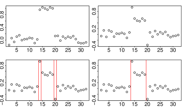
Figure 1: Top left: a series around two changes, with $\rho^{\star}=0.5$. Top right: the decorrelated series in the same region. Bottom left: before post-processing, two pairs of adjacent change-points are found. Bottom right: post-processing removes the last change-point of each pair of adjacent ones.

In practice, it may also be useful to have some guidance on how to check that the assumptions underpinning our approach are satisfied for a given data set. A possible approach is to subtract the estimated piecewise constant function from the original series. If the model is the expected one, this new series should be a realization of an AR(1) Gaussian process. Hence, the residuals built by decorrelation of this series should be Gaussian and independent. One way to check this is to perform a gaussianity test and a Portmanteau test on this series of residuals.

5.2 Simulation design

To assess the performance of the proposed method, we used a simulation design inspired from the one conceived by [19]. We considered series of length $n\in\{100,200,400,800,1600\}$ with autocorrelation at lag 1, denoted by $\rho^{\star}$, ranging from $-.9$ to $.9$ (by steps of $.1$) and residual standard deviation $\sigma^{\star}$ between $.1$ and $.6$ (by steps of $.1$). All series were affected by $m^{\star}=6$ change-points located at fractions $1/6\pm 1/36,3/6\pm 2/36,5/6\pm 3/36$ of their length. Each combination was replicated $S=100$ times. The mean within each segment alternates between 0 and 1, starting with $\mu_{1}=0$.

Estimation of $\rho^{\star}$.

For each generated series, two different estimates $\overline{\rho}_{n}$ of $\rho^{\star}$ were computed: the original estimate $\overline{\rho}_{n}=\widehat{\rho}_{\textrm{MG}}$ proposed by [27] and our revised version $\overline{\rho}_{n}=\widetilde{\rho}_{n}$. We carried the same study on series with no change-point (centered series).

Estimation of the segmentation parameters.

For each generated series, we estimated the change-point locations $\widehat{\boldsymbol{\tau}}_{n}(y,\overline{\rho}_{n})$ using Proposition 2 for each $m$ from $1$ to $m_{\max}=75$ and with different choices of $\overline{\rho}_{n}$: $\widetilde{\rho}_{n}$ (our estimator), $\rho^{\star}$ (the true value) and zero (which does not take into account for the autocorrelation). For each choice of $\overline{\rho}_{n}$, we then selected the number of change-points $\hat{m}$ using (17). Actually, the last choice $\overline{\rho}_{n}=0$ corresponds to the classical least-squares framework. In addition, we shall also use the post-processing described in Section 5.1 for the cases where $\overline{\rho}_{n}=\widetilde{\rho}_{n}$ and $\rho^{\star}$.
To study the quality of the proposed model selection criterion, we computed the distribution of $\widehat{m}$ for each estimate $\overline{\rho}_{n}\in\{\widetilde{\rho}_{n},\rho^{\star},0\}$ with post-processing or not for the first two estimates of $\rho^{\star}$.

In order to assess the performance of the estimation of the change-point locations, we computed the Hausdorff distance defined in the segmentation framework as follows, see [7] and [16]:

$$d\left(\boldsymbol{\tau}^{\star},\widehat{\boldsymbol{\tau}}_{n}\left(y,\overline{\rho}_{n}\right)\right)=\max\left(d_{1}\left(\boldsymbol{\tau}^{\star},\widehat{\boldsymbol{\tau}}_{n}\left(y,\overline{\rho}_{n}\right)\right),d_{2}\left(\boldsymbol{\tau}^{\star},\widehat{\boldsymbol{\tau}}_{n}\left(y,\overline{\rho}_{n}\right)\right)\right)\;,$$ (19)

where

$$d_{1}\left(\boldsymbol{a},\boldsymbol{b}\right) = \underset{b\in\boldsymbol{b}}{\sup}\underset{a\in\boldsymbol{a}}{\inf}\left|a-b\right|,$$ (20)

$$\text{and \qquad}d_{2}\left(\boldsymbol{a},\boldsymbol{b}\right) = d_{1}\left(\boldsymbol{b},\boldsymbol{a}\right).$$ (21)

$d_{1}$ close to zero means that an estimated change-point is likely to be close to a true change-point. A small value of $d_{2}$ means that a true change-point is likely to be close to each estimated change-point. A perfect segmentation results in both null $d_{1}$ and $d_{2}$. Over-segmentation results in a small $d_{1}$ and a large $d_{2}$. Under-segmentation results in a large $d_{1}$ and a small $d_{2}$, provided that the estimated change-points are correctly located.

5.3 Results

Estimation of $\rho^{\star}$.

In Figure 2, we compare the performance of our robust estimator of $\rho^{\star}$: $\widetilde{\rho}_{n}$ with the ones of the estimator $\widehat{\rho}_{\textrm{MG}}$ in the case where there are no change-points in the observations. More precisely, in this case, the observations $y$ are generated under the model (1) with $\mu_{k}^{\star}=0$, for all $k$. We observe that the estimator proposed by [27] performs better than our robust estimator. However, it is not the case anymore in the presence of change-points in the data as we can see in Figure 3. In the latter case, our robust estimator $\widetilde{\rho}_{n}$ outperforms the estimator $\widehat{\rho}_{\textrm{MG}}$ for almost all values of $\rho^{\star}$.

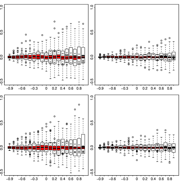
Figure 2: Boxplots of $\widehat{\rho}_{\textrm{MG}}-\rho^{\star}$ in red and $\widetilde{\rho}_{n}-\rho^{\star}$ in black for different values of $\rho^{\star}$ in the case where there are no change-points in the data with $n=400$ (plots on the left), $n=1600$ (plots on the right), $\sigma^{\star}=0.2$ (top) and $\sigma^{\star}=0.6$ (bottom).

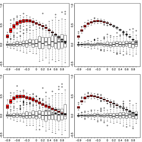
Figure 3: Boxplots of $\widehat{\rho}_{\textrm{MG}}-\rho^{\star}$ in red and $\widetilde{\rho}_{n}-\rho^{\star}$ in black for different values of $\rho^{\star}$ in the case where there are change-points in the data with $n=400$ (plots on the left), $n=1600$ (plots on the right), $\sigma^{\star}=0.2$ (top) and $\sigma^{\star}=0.6$ (bottom).

Model selection.

In Figures 4 and 5, we compare the estimated number of change-points $\widehat{m}$ in two different configurations of signal-to-noise ratio ($\sigma^{\star}=0.1$ and $\sigma^{\star}=0.5$) and with three different values of $\rho^{\star}$ ($\rho^{\star}=0.3$, $0.6$ and $0.8$). In this figures, the notation LS, Robust and Oracle correspond to the cases where $\overline{\rho}_{n}=0$, $\overline{\rho}_{n}=\tilde{\rho}_{n}$ and $\overline{\rho}_{n}=\rho^{\star}$, respectively. Moreover, we use the notation -P when the post-processing described in Section 5.1 is used. In the situations where $\sigma^{\star}$ and $\rho^{\star}$ are small, all the methods provide an accurate estimation of the number of change-points. In the other cases, LS tends to strongly overestimate the number of change-points. Robust and Oracle tend to select twice the true number of change-points due to the artifactual presence of change-points in the decorrelated series as explained in Section 5.1. This is corrected by the post-processing and Robust-P provides the correct number of change-points in most of the considered configurations. Moreover, we also observe that the performance of Robust and Robust-P are similar to these of Oracle and Oracle-P: the robust decorrelation procedure we propose performs as well as if $\rho^{\star}$ was known for $n=1600$. It has to be noted that the post-processing would not improve the performance on LS so we did not considered it.

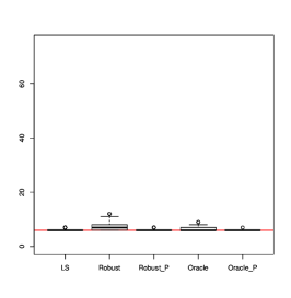
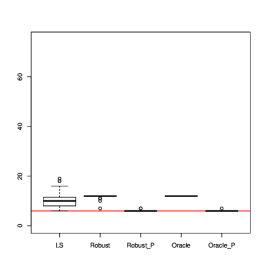
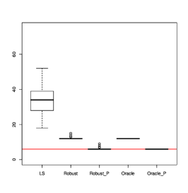
Figure 4: Boxplots for the estimated number of change-points for $n=1600$ when $\overline{\rho}_{n}=0$ (LS), $\overline{\rho}_{n}=\tilde{\rho}_{n}$ (Robust and Robust-P with post-processing) and $\overline{\rho}_{n}=\rho^{\star}$ (Oracle and Oracle-P with post-processing) with $\sigma^{\star}=0.1$ and $\rho^{\star}=0.3$ (left), $\rho^{\star}=0.6$ (middle) and $\rho^{\star}=0.8$ (right). The true number of change-points is equal to 6 (red horizontal line).

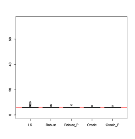
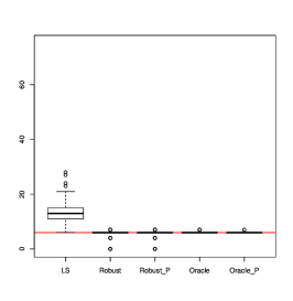
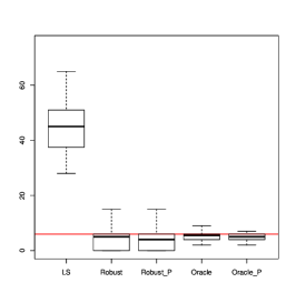
Figure 5: Boxplots for the estimated number of change-points for $n=1600$ when $\overline{\rho}_{n}=0$ (LS), $\overline{\rho}_{n}=\tilde{\rho}_{n}$ (Robust and Robust-P with post-processing) and $\overline{\rho}_{n}=\rho^{\star}$ (Oracle and Oracle-P with post-processing) with $\sigma^{\star}=0.5$ and $\rho^{\star}=0.3$ (left), $\rho^{\star}=0.3$ (middle) and $\rho^{\star}=0.8$ (right). The true number of change-points is equal to 6 (red horizontal line).

Change-point locations.

In Figures 6 and 8 are displayed the boxplots of the two parts $d_{1}$ and $d_{2}$ of the Hausdorff distance defined in (20) and (21), respectively for different values of $\rho^{\star}$ when $\sigma^{\star}=0.5$. $d_{2}$ is displayed in Figure 7 for $\sigma^{\star}=0.1$; for this value of $\sigma^{\star}$, $d_{1}$ was found null for all methods and all values of $\rho^{\star}$.

When the noise is small ($\sigma^{\star}=0.1$), the robust procedure we propose performs well for the whole range of correlation. On the contrary, the performance of LS are deprecated when the correlation increases, whereas these of LS^⋆ still provide accurate change-point locations. This shows that the least-square approach only fails because it turns to overestimate the number of change-points. This is all the more true for LS when the variance of the noise is large ($\sigma^{\star}=0.5$). When the problem gets difficult (both $\sigma^{\star}$ and $\rho^{\star}$ large), our robust procedure tends to underestimate the number of change-points (which was expected) and the estimated change-points are close to true ones.

Figure 6: Boxplots for the first part of the Hausdorff distance ($d_{1}$) for $n=1600$ when $\overline{\rho}_{n}=0$ (LS and LS* when the true number of change-points is known), $\overline{\rho}_{n}=\tilde{\rho}_{n}$ (Robust and Robust-P with post-processing) and $\overline{\rho}_{n}=\rho^{\star}$ (Oracle and Oracle-P with post-processing) with $\sigma^{\star}=0.5$ and $\rho^{\star}=0.3$ (left), $\rho^{\star}=0.6$ (middle) and $\rho^{\star}=0.8$ (right).

Figure 7: Boxplots for the second part of the Hausdorff distance ($d_{2}$) for $n=1600$ when $\overline{\rho}_{n}=0$ (LS and LS* when the true number of change-points is known), $\overline{\rho}_{n}=\tilde{\rho}_{n}$ (Robust and Robust-P with post-processing) and $\overline{\rho}_{n}=\rho^{\star}$ (Oracle and Oracle-P with post-processing) with $\sigma^{\star}=0.1$ and $\rho^{\star}=0.3$ (left), $\rho^{\star}=0.6$ (middle) and $\rho^{\star}=0.8$ (right).

Figure 8: Boxplots for the second part of the Hausdorff distance ($d_{2}$) when $\overline{\rho}_{n}=0$ (LS and LS* when the true number of change-points is known), $\overline{\rho}_{n}=\tilde{\rho}_{n}$ (Robust and Robust-P with post-processing) and $\overline{\rho}_{n}=\rho^{\star}$ (Oracle and Oracle-P with post-processing) with $\sigma^{\star}=0.5$ and $\rho^{\star}=0.3$ (left), $\rho^{\star}=0.6$ (middle) and $\rho^{\star}=0.8$ (right).

An other way to illustrate the performance of the estimation of the change-point locations is the histograms of these estimates. We provide these plots only for LS, Robust-P and Oracle-P, because Post-processing does not change significantly LS estimates, and, furthermore, Robust (resp. Oracle) method’s histograms with or without Post-Processing are very similar, see Figures 9 and 10.

These figures illustrate that in case of over-estimation of the number of changes by LS method, the additional change-points seem to be uniformly distributed.

Figure 9: Frequencies of each possible change-point estimator, with $\sigma^{\star}=0.1$ and $n=1600$. Tick-marks on bottom-side axis represent the true change-point locations. $\overline{\rho}_{n}=0$ (LS, top line), $\overline{\rho}_{n}=\tilde{\rho}_{n}$ (Robust-P, middle line) and $\overline{\rho}_{n}=\rho^{\star}$ (Oracle-P, bottom line) with $\rho^{\star}=0.3$ (left), $\rho^{\star}=0.6$ (middle) and $\rho^{\star}=0.8$ (right).

Figure 10: Frequencies of each possible change-point estimator, with $\sigma^{\star}=0.5$ and $n=1600$. Tick-marks on bottom-side axis represent the true change-point locations.$\overline{\rho}_{n}=0$ (LS, top line), $\overline{\rho}_{n}=\tilde{\rho}_{n}$ (Robust-P, middle line) and $\overline{\rho}_{n}=\rho^{\star}$ (Oracle-P, bottom line) with $\rho^{\star}=0.3$ (left), $\rho^{\star}=0.6$ (middle) and $\rho^{\star}=0.8$ (right).

5.4 Additional simulation studies

5.4.1 Comparison with Bardet et al. [5]

The quasi-maximum likelihood method proposed by [5], when applied to a Gaussian AR(1) process with changes in the mean $\left(y_{0},\dots,y_{n}\right)$ , consists in the minimization wrt $\boldsymbol{\rho}=\left(\rho_{0},\dots,\rho_{m}\right),\boldsymbol{\sigma}=\left(\sigma_{0},\dots,\sigma_{m}\right),\boldsymbol{\delta}=\left(\delta_{0},\dots,\delta_{m}\right)$ and $\boldsymbol{t}=\left(t_{0},\dots,t_{m}\right)$ of the following function:

$$\left(\boldsymbol{\rho},\boldsymbol{\sigma},\boldsymbol{\delta},\boldsymbol{t}\right)\mapsto\sum_{k=0}^{m}\left\{\left(t_{k+1}-t_{k}\right)\log\left(\sigma_{k}^{2}\right)+\frac{1}{\sigma_{k}^{2}}\sum_{i=t_{k}+1}^{t_{k+1}}\left(y_{i}-\rho_{k}y_{i-1}-\delta_{k}\right)^{2}\right\}\;.$$ (22)

Indeed, in the class of models considered in [5], changes in all the parameters are possible at each change-point. Using this method to estimate the change-point locations for data satisfying Model (1) or (8) boils down to ignore the stationarity of $\left(\eta_{i}\right)_{i\geq 0}$ as defined in (2). It can lead to a poor estimation of change-point locations, especially when there are many changes close to each other. To illustrate this fact, we compared our estimator of change-point locations to the estimates given by the minimization of (22). We generated $100$ series of length $400$, under Model (1), with $\rho^{\star}=0.3$ and $\sigma^{\star}=0.4$. The number of change-points, their locations and the means within segments are the same as in Section 5.2. The number of changes is assumed to be known and we did not post-process the estimates. Simulations show that using the method of [5] in this case can lead to a poor estimation of close change-points, while our method is less affected by the length of segments (see Figure 11). For example, the boundaries of the smallest segment are recovered in less than half of the simulations when minimizing (22).

Figure 11: Frequencies of each possible change-point location estimate. Tick-marks on bottom-side axis represent the true change-point locations. Left: Estimation by the minimization of (22). Right: Our method.

5.4.2 Robustness to model mis-specification

In this section, we study the behaviour of our proposed robust procedure (Robust-P) when the signal is corrupted by an AR(2) Gaussian process, e.g. in Model 1, $\eta_{i}$ is a zero-mean stationary process such that

$$\eta_{i}=\phi_{1}^{\star}\eta_{i-1}+\phi_{2}^{\star}\eta_{i-2}+\varepsilon_{i},$$

where $|\phi_{2}|<1$, $\phi_{1}+\phi_{2}<1$ and $\phi_{2}-\phi_{1}<1$. We considered series of fixed length $n=1600$, a residual standard deviation $\sigma^{\star}=0.1$, $\phi_{1}^{\star}=0.3$ and $\phi_{2}^{\star}$ in $\{-0.9,-0.8,-0.7,\dots,0.5,0.6\}$ We used the same segmentation design as in subsection 5.1. Each combination was replicated $100$ times. All the results are displayed in Figure 12.
The procedure performs well when $\phi_{2}^{\star}$ belongs to the interval $[-0.5,0.2]$ as expected (similar to the case of AR(1)): the estimated segmentation is close to the true one. When $\phi_{2}^{\star}>0.2$, it tends to over-estimate the number of change-points. The true change-points are detected ($d_{1}$ is close to zero, e.g. the decorrelation procedure with the obtained negative estimation of ${\rho}^{\star}$ leads to an increasing in the mean differences) but false change-points are added (large $d_{2}$). When $\phi_{2}^{\star}<-0.5$, under-segmentation is observed: the decorrelation procedure with a large estimated value of ${\rho}^{\star}$ leads to a difficult segmentation problem.

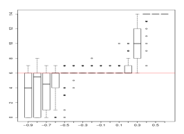
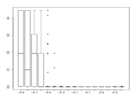
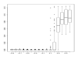
Figure 12: Left: Boxplots for the estimated number of change-points. Center and right: Boxplots for the first part of the Hausdorff distance ($d_{1}$) and for the second part of the Hausdorff distance ($d_{2}$) with $n=1600$, $\sigma^{\star}=0.1$ and $\phi_{1}^{\star}=0.3$ wrt different values of $\phi_{2}^{\star}$.

5.4.3 Estimator of $\rho^{\star}$ in the case of the Cauchy distribution

In Section 2, an analogous estimator of $\rho^{\star}$ in the case of Cauchy distributed observations is proposed. We follow the simulation design described in Subsection 5.2, where the Gaussian random variables are replaced by Cauchy random variables. More precisely, the expectation parameters are replaced by the location parameters of the Cauchy distribution and $\sigma^{\star}$ is replaced by the scale parameter of the Cauchy distribution. We can see from Figure 13 that $\widetilde{\widetilde{\rho}}_{n}$ is an accurate estimator of $\rho^{\star}$ except when $\rho^{\star}$ is close to zero.

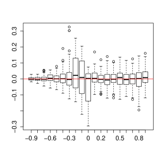
Figure 13: Boxplots of $\widetilde{\widetilde{\rho}}_{n}-\rho^{\star}$ for different values of $\rho^{\star}$ when $n=1600$ and $\sigma^{\star}=0.1$.

When this estimator of $\rho^{\star}$ is used in our change-point estimation method, it leads to poor estimations of the change-points since the Cauchy distribution does not have finite second order moment (simulations not shown).

6 Conclusion

In this paper, we propose a novel approach for estimating multiple change-points in the mean of a Gaussian AR(1) process. Our approach is based on two main stages. The first one consists in building a robust estimator of the autocorrelation parameter which is used for whitening the original series. In the second stage, we apply the inference approach commonly used to estimate change-points in the mean of independent random variables. In the course of this study, we have shown that our approach, which is implemented in the R package AR1seg, is a very efficient technique both on a theoretical and practical point of view. More precisely, it has two main features which make it very attractive. Firstly, the estimators that we propose have the same asymptotic properties as the classical estimators in the independent framework which means that the performances of our estimators are not affected by the dependence assumption. Secondly, from a practical point of view, AR1seg is computationally efficient and exhibits better performance on finite sample size data than existing approaches which do not take into account the dependence structure of the observations.

Appendix A Proofs

A.1 Proof of Proposition 1

Let $F_{1}$ and $F_{2}$ denote the cumulative distribution functions (cdf) of $\left(\left|y_{i+1}-y_{i}\right|\right)$ for $i\neq t_{n,1}^{\star},\dots,t_{n,m^{\star}}^{\star}$ and $\left(|y_{i+2}-y_{i}|\right)$ for $i\neq t_{n,1}^{\star}-1,\dots,t_{n,m^{\star}}^{\star}-1$, respectively. By (1), $(y_{i}-\mathbb{E}(y_{i}))_{0\leq i\leq n}$ are $(n+1)$ observations of a AR(1) stationnary Gaussian process thus for any $i\neq t_{n,1}^{\star},\dots,t_{n,m^{\star}}^{\star}$, $(y_{i+1}-y_{i})$ and for any $i\neq t_{n,1}^{\star}-1,\dots,t_{n,m^{\star}}^{\star}-1$, $(y_{i+2}-y_{i})$ are zero-mean Gaussian random variables with variances equal to $2\sigma^{\star 2}/(1+\rho^{\star})$ and $2\sigma^{\star 2}$, respectively. Hence, for all $t$ in $\mathbb{R}$,

$$F_{1}:t\mapsto 2\Phi\left(t\sqrt{\frac{1+\rho^{\star}}{2\sigma^{\star 2}}}\right)-1\textrm{ and }F_{2}:t\mapsto 2\Phi\left(t\sqrt{\frac{1}{2\sigma^{\star 2}}}\right)-1\;,$$ (23)

where $\Phi$ denotes the cumulative distribution function of a standard Gaussian random variable.

Let also denote by $F_{1,n}$ and $F_{2,n-1}$ the empirical cumulative distribution functions of $\left(|y_{i+1}-y_{i}|\right)_{0\leq i\leq n-1}$ and $\left(|y_{i+2}-y_{i}|\right)_{0\leq i\leq n-2}$, respectively. Observe that for all $t$ in $\mathbb{R}$,

$$\sqrt{n}(F_{1,n}(t)-F_{1}(t))=\frac{1}{\sqrt{n}}\sum_{i=0}^{n-1}\left(\mathbbm{1}_{\{|y_{i+1}-y_{i}|\leq t\}}-F_{1}(t)\right)\\ =\frac{1}{\sqrt{n}}\sum_{i\in\{t_{n,1}^{\star},\dots,t_{n,m^{\star}}^{\star}\}}\left(\mathbbm{1}_{\{|y_{i+1}-y_{i}|\leq t\}}-F_{1}(t)\right)+\frac{1}{\sqrt{n}}\sum_{\stackrel{{\scriptstyle 0\leq i\leq n-1}}{{i\notin\{t_{n,1}^{\star},\dots,t_{n,m^{\star}}^{\star}\}}}}\left(\mathbbm{1}_{\{|y_{i+1}-y_{i}|\leq t\}}-F_{1}(t)\right)\\ =\frac{1}{\sqrt{n}}\sum_{0\leq i\leq n-1}\left(\mathbbm{1}_{\{|z_{i}|\leq t\}}-F_{1}(t)\right)+R_{n}(t)\;,$$ (24)

where $\sup_{t\in\mathbb{R}}|R_{n}(t)|=o_{p}(1)$, the $z_{i}=y_{i+1}-y_{i}$ except for $i=t_{n,1}^{\star},\dots,t_{n,m^{\star}}^{\star}$, where $z_{i}=\eta_{i+1}-\eta_{i}$, $(\eta_{i})$ being defined in (2).

Thus, by using the theorem of [11], we obtain that the first term in the rhs of (24) converges in distribution to a zero-mean Gaussian process $G$ in the space of càdlàg functions equipped with the uniform norm. Since the second term in the rhs tends uniformly to zero in probability, we get that $\sqrt{n}(F_{1,n}-F_{1})$ converges in distribution to a zero-mean Gaussian process in the space of càdlàg functions equipped with the uniform norm and that the same holds for $\sqrt{n-1}(F_{2,n-1}-F_{2})$.

By Lemma 21.3 of [33] the quantile function $T:F\mapsto F^{-1}(1/2)$ is Hadamard differentiable at $F$ tangentially to the set of càdlàg functions $h$ that are continuous at $F^{-1}(1/2)$ with derivative $T^{\prime}_{F}(h)=-h(F^{-1}(1/2))/F^{\prime}(F^{-1}(1/2))$. By applying the functional delta method (Theorem 20.8 in [33]), we get that $\sqrt{n}(T(F_{1,n})-T(F_{1}))$ converges in distribution to $T^{\prime}_{F_{1}}(G)$. Moreover, by the continuous mapping theorem, it is the same for $T^{\prime}_{F_{1}}\left\{\sqrt{n}(F_{1,n}-F_{1})\right\}$. Thus,

$$\sqrt{n}\left(F^{-1}_{1,n}(1/2)-F_{1}^{-1}(1/2)\right)=T^{\prime}_{F_{1}}\left\{\sqrt{n}(F_{1,n}-F_{1})\right\}+o_{p}(1)\\ =-\frac{1}{\sqrt{n}}\frac{\sum_{i=0}^{n-1}\left(\mathbbm{1}_{\{|y_{i+1}-y_{i}|\leq F_{1}^{-1}(1/2)\}}-1/2\right)}{F_{1}^{\prime}(F_{1}^{-1}(1/2))}+o_{p}(1)\;.$$ (25)

In the same way,

$$\sqrt{n-1}\left(F^{-1}_{2,n-1}(1/2)-F_{2}^{-1}(1/2)\right)=\\ -\frac{1}{\sqrt{n-1}}\frac{\sum_{i=0}^{n-2}\left(\mathbbm{1}_{\{|y_{i+2}-y_{i}|\leq F_{2}^{-1}(1/2)\}}-1/2\right)}{F_{2}^{\prime}(F_{2}^{-1}(1/2))}+o_{p}(1)\;,$$ (26)

By applying the Delta method [33, Theorem 3.1] with the transformation $f(x)=x^{2}$, we get

$$\sqrt{n}\left(F^{-1}_{1,n}(1/2)^{2}-F_{1}^{-1}(1/2)^{2}\right)=\\ -\frac{2F_{1}^{-1}(1/2)}{\sqrt{n}}\frac{\sum_{i=0}^{n-1}\left(\mathbbm{1}_{\{|y_{i+1}-y_{i}|\leq F_{1}^{-1}(1/2)\}}-1/2\right)}{F_{1}^{\prime}(F_{1}^{-1}(1/2))}+o_{p}(1)\;,$$ (27)

$$\sqrt{n-1}\left(F^{-1}_{2,n-1}(1/2)^{2}-F_{2}^{-1}(1/2)^{2}\right)=\\ -\frac{2F_{2}^{-1}(1/2)}{\sqrt{n-1}}\frac{\sum_{i=0}^{n-2}\left(\mathbbm{1}_{\{|y_{i+2}-y_{i}|\leq F_{2}^{-1}(1/2)\}}-1/2\right)}{F_{2}^{\prime}(F_{2}^{-1}(1/2))}+o_{p}(1)\;,$$ (28)

Note that by (23), we obtain that

$$F_{1}^{-1}(1/2)=\sqrt{\frac{2\sigma^{\star 2}}{1+\rho^{\star}}}\Phi^{-1}(3/4)\textrm{ and }F_{2}^{-1}(1/2)=\sqrt{2\sigma^{\star 2}}\Phi^{-1}(3/4)\;.$$ (29)

Moreover,

$$F_{1}^{\prime}(F_{1}^{-1}(1/2))=2\sqrt{\frac{1+\rho^{\star}}{2\sigma^{\star 2}}}\varphi\left(\Phi^{-1}(3/4)\right)\textrm{ and }F_{2}^{\prime}(F_{2}^{-1}(1/2))=2\sqrt{\frac{1}{2\sigma^{\star 2}}}\varphi\left(\Phi^{-1}(3/4)\right)\;,$$ (30)

where $\varphi$ denotes the p.d.f of a standard Gaussian random variable.

Observe that $\sqrt{n}(\widetilde{\rho}_{n}-\rho^{\star})$ can be rewritten as follows:

$$\sqrt{n}(\widetilde{\rho}_{n}-\rho^{\star})=\sqrt{n}\;\frac{F^{-1}_{2,n}(1/2)^{2}-(1+\rho^{\star})F^{-1}_{1,n}(1/2)^{2}}{F^{-1}_{1,n}(1/2)^{2}}\\ =\sqrt{n}\;\frac{\left(F^{-1}_{2,n-1}(1/2)^{2}-F_{2}^{-1}(1/2)^{2}\right)-(1+\rho^{\star})\left(F^{-1}_{1,n}(1/2)^{2}-F_{1}^{-1}(1/2)^{2}\right)}{F^{-1}_{1,n}(1/2)^{2}}\\ +\sqrt{n}\;\frac{F_{2}^{-1}(1/2)^{2}-(1+\rho^{\star})F_{1}^{-1}(1/2)^{2}}{F^{-1}_{1,n}(1/2)^{2}}\;.$$ (31)

By (29) the last term in the rhs of (31) is equal to zero. Thus,

$$\sqrt{n}(\widetilde{\rho}_{n}-\rho^{\star})=\\ \frac{1}{\sqrt{n-1}}\sum_{i=0}^{n-2}\left\{a_{2}\left(\mathbbm{1}_{\{|y_{i+2}-y_{i}|\leq F_{2}^{-1}(1/2)\}}-1/2\right)-a_{1}(1+\rho^{\star})\left(\mathbbm{1}_{\{|y_{i+1}-y_{i}|\leq F_{1}^{-1}(1/2)\}}-1/2\right)\right\}+o_{p}(1)\;,$$

where, by (30),

$$a_{2} = -\frac{2F_{2}^{-1}(1/2)}{F_{2}^{\prime}(F_{2}^{-1}(1/2))}=-2\sigma^{\star 2}\frac{\Phi^{-1}(3/4)}{\varphi\left(\Phi^{-1}(3/4)\right)}$$

$$\textrm{ and }a_{1} = -\frac{2F_{1}^{-1}(1/2)}{F_{1}^{\prime}(F_{1}^{-1}(1/2))}=-\frac{2\sigma^{\star 2}}{1+\rho^{\star}}\frac{\Phi^{-1}(3/4)}{\varphi\left(\Phi^{-1}(3/4)\right)}\;.$$

By (29), $\sqrt{n}(\widetilde{\rho}_{n}-\rho^{\star})$ can thus be rewritten as follows:

$$\sqrt{n}(\widetilde{\rho}_{n}-\rho^{\star})=\frac{1}{\sqrt{n-1}}\sum_{0\leq i\leq n-2}\Psi(\eta_{i},\eta_{i+1},\eta_{i+2})+o_{p}(1)\;.$$

where $\Psi$ is defined in (5) and $(\eta_{i})$ is defined in (2). Since $\Psi$ is a function on $\mathbb{R}^{3}$ with Hermite rank greater than 1 and $(\eta_{i})_{i\geq 0}$ is a stationary AR(1) Gaussian process, (4) follows by applying [1, Theorem 4].

A.2 Hints for (6)

Note that if $X$ has a Cauchy($x_{0}$,$\gamma$) distribution then the characteristic function $\varphi_{X}$ of $X$ can be written as $\varphi_{X}(t)=\mathrm{e}^{\mathrm{i}x_{0}t-\gamma|t|}.$ Moreover, the cdf $F_{X}$ of $X$ is such that $F_{X}^{-1}(3/4)=x_{0}+\gamma$. Thus, $\eta_{i}=\sum_{k\geq 0}(\rho^{\star})^{k}\varepsilon_{i-k}$ has a Cauchy$\left(\frac{x_{0}}{1-\rho^{\star}},\frac{\gamma}{1-|\rho^{\star}|}\right)$ distribution and $(\rho^{\star}-1)\eta_{i}$ has a Cauchy$\left(-x_{0},\frac{\gamma|\rho^{\star}-1|}{1-|\rho^{\star}|}\right)$ distribution. Since $\eta_{i+1}-\eta_{i}=(\rho^{\star}-1)\eta_{i}+\varepsilon_{i}$ is a sum of two independent Cauchy random variables, it is distributed as a Cauchy$\left(0,\gamma\left(1+\left|\frac{\rho^{\star}-1}{1-|\rho^{\star}|}\right|\right)\right)$ distribution. In the same way, $\eta_{i+2}-\eta_{i}=({\rho^{\star}}^{2}-1)\eta_{i}+\rho^{\star}\varepsilon_{i}+\varepsilon_{i+2}$ is a sum of three independent Cauchy random variables and has thus a Cauchy$\left(0,2\gamma(1+|\rho^{\star}|)\right)$. Let $F_{1}$ and $F_{2}$ denote the cdf of $(\eta_{i+1}-\eta_{i})$ and $(\eta_{i+2}-\eta_{i})$, respectively. By using the properties of the cdf of a Cauchy distribution, we get, on the one hand, that $F_{2}^{-1}(3/4)=2\gamma(1+|\rho^{\star}|)$ and, on the other hand, that

$$F_{1}^{-1}(3/4)=\left\{\begin{array}[]{cc}2\gamma,&\textrm{if }\rho^{\star}>0\;,\\ \frac{2\gamma}{1+\rho^{\star}},&\textrm{if }\rho^{\star}<0\;.\end{array}\right.$$

From this we get that

$$\left(\frac{F_{2}^{-1}(3/4)}{F_{1}^{-1}(3/4)}\right)^{2}-1=\left\{\begin{array}[]{cc}\rho^{\star}(2+\rho^{\star}),&\textrm{if }\rho^{\star}>0\;,\\ {\rho^{\star}}^{2}({\rho^{\star}}^{2}-2),&\textrm{if }\rho^{\star}<0\;.\end{array}\right.$$ (32)

The definition of $\widetilde{\widetilde{\rho}}_{n}$ comes by inverting these last two functions.

A.3 Proof of Proposition 2

In the sequel, we need the following definitions, notations and remarks. Observe that (8) can be rewritten as follows:

$$z=\rho^{*}Bz+T\left(\boldsymbol{t}_{n}^{\star}\right)\boldsymbol{\delta}^{\star}+\epsilon\;,$$ (33)

where

$$z=\left(\begin{array}[]{c}z_{1}\\ \vdots\\ z_{n}\end{array}\right)\;,\qquad Bz=\left(\begin{array}[]{c}z_{0}\\ \vdots\\ z_{n-1}\end{array}\right)\;,\qquad\boldsymbol{\delta}^{\star}=\left(\begin{array}[]{c}\delta^{\star}_{0}\\ \vdots\\ \delta^{\star}_{m}\end{array}\right)\;,\qquad\epsilon=\left(\begin{array}[]{c}\epsilon_{1}\\ \vdots\\ \epsilon_{n}\end{array}\right)\;,$$ (34)

where $\delta_{k}^{\star}=(1-\rho^{\star})\mu^{\star}_{k}$, for $0\leq k\leq m$, and $T\left(\boldsymbol{t}\right)$ is an $n\times(m+1)$ matrix where the $k$th column is $(\underset{t_{k-1}}{\underbrace{0,\dots,0}}\;\underset{t_{k}-t_{k-1}}{\underbrace{1,\dots,1}}\;\underset{n-t_{k}}{\underbrace{0,\dots,0}})^{\prime}$. Let us define the exact and estimated decorrelated series by

$$w^{\star} = z-\rho^{\star}Bz\;,$$ (35)

$$\overline{w} = z-\overline{\rho}_{n}Bz\;.$$ (36)

For any vector subspace $E$ of $\mathbb{R}^{n}$, let $\pi_{E}$ denote the orthogonal projection of $\mathbb{R}^{n}$ on $E$. Let also $\|\cdot\|$ be the euclidian norm on $\mathbb{R}^{n}$, $\langle\cdot,\cdot\rangle$ the canonical scalar product on $\mathbb{R}^{n}$ and $\|\cdot\|_{\infty}$ the sup norm. For $x$ a vector of $\mathbb{R}^{n}$ and $\boldsymbol{t}\in\mathcal{A}_{n,m}$, let

$$J_{n,m}\left(x,\boldsymbol{t}\right)=\frac{1}{n}\left(\|\pi_{E_{\boldsymbol{t}_{n}^{\star}}}\left(x\right)\|^{2}-\|\pi_{E_{\boldsymbol{t}}}\left(x\right)\|^{2}\right)\;,$$ (37)

written $J_{n}\left(x,\boldsymbol{t}\right)$ in the sequel for notational simplicity. In (37), $E_{\boldsymbol{t}_{n}^{\star}}$ and $E_{\boldsymbol{t}}$ correspond to the linear subspaces of $\mathbb{R}^{n}$ generated by the columns of $T\left(\boldsymbol{t}_{n}^{\star}\right)$ and $T\left(\boldsymbol{t}\right)$, respectively. We shall use the same decomposition as the one introduced in [22]:

$$J_{n}\left(x,\boldsymbol{t}\right)=K_{n}\left(x,\boldsymbol{t}\right)+V_{n}\left(x,\boldsymbol{t}\right)+W_{n}\left(x,\boldsymbol{t}\right)\;,$$ (38)

where

$$K_{n}\left(x,\boldsymbol{t}\right) = \frac{1}{n}\left\|\left(\pi_{E_{\boldsymbol{t}_{n}^{\star}}}-\pi_{E_{\boldsymbol{t}}}\right)\mathbb{E}x\right\|^{2}\;,$$ (39)

$$V_{n}\left(x,\boldsymbol{t}\right) = \frac{1}{n}\left(\left\|\pi_{E_{\boldsymbol{t}_{n}^{\star}}}\left(x-\mathbb{E}x\right)\right\|^{2}-\left\|\pi_{E_{\boldsymbol{t}}}\left(x-\mathbb{E}x\right)\right\|^{2}\right)\;,$$ (40)

$$W_{n}\left(x,\boldsymbol{t}\right) = \frac{2}{n}\left(\left\langle\pi_{E_{\boldsymbol{t}_{n}^{\star}}}\left(x-\mathbb{E}x\right),\pi_{E_{\boldsymbol{t}_{n}^{\star}}}\left(\mathbb{E}x\right)\right\rangle-\left\langle\pi_{E_{\boldsymbol{t}}}\left(x-\mathbb{E}x\right),\pi_{E_{\boldsymbol{t}}}\left(\mathbb{E}x\right)\right\rangle\right)\;.$$ (41)

We shall also use the following notations:

$$\underline{\lambda} = \underset{1\leq k\leq m}{\min}\left|\delta_{k}^{\star}-\delta_{k-1}^{\star}\right|\;,$$ (42)

$$\overline{\lambda} = \underset{1\leq k\leq m}{\max}\left|\delta_{k}^{\star}-\delta_{k-1}^{\star}\right|\;,$$ (43)

$$\Delta_{\boldsymbol{\tau}^{\star}} = \underset{1\leq k\leq m+1}{\min}\left(\tau_{k}^{\star}-\tau_{k-1}^{\star}\right)\;,$$ (44)

$$\mathcal{C}_{\nu,\gamma,n,m} = \left\{\boldsymbol{t}\in\mathcal{A}_{n,m};\nu\underline{\lambda}^{-2}\leq\|\boldsymbol{t}-\boldsymbol{t}_{n}^{\star}\|\leq n\gamma\Delta_{\boldsymbol{\tau}^{\star}}\right\}\;,$$ (45)

$$\mathcal{C}_{\nu,\gamma,n,m}^{\prime} = \mathcal{C}_{\nu,\gamma,n,m}\cap\left\{\boldsymbol{t}\in\mathcal{A}_{n,m};\forall k=1,\dots,m,t_{k}\geq t_{n,k}^{\star}\right\}\;,$$ (46)

$$\mathcal{C}_{\nu,\gamma,n,m}^{\prime}\left(\mathcal{I}\right) = \left\{\boldsymbol{t}\in\mathcal{C}_{\nu,\gamma,n,m}^{\prime};\right.$$ (47)

$$\left.\forall k\in\mathcal{I},\nu\underline{\lambda}^{-2}\leq t_{k}-t_{n,k}^{\star}\leq n\gamma\Delta_{\boldsymbol{\tau}^{\star}}\textit{ and }\forall k\notin\mathcal{I},t_{k}-t_{n,k}^{\star}<\nu\underline{\lambda}^{-2}\right\}\;,$$

for any $\nu>0$, $0<\gamma<1/2$ and $\mathcal{I}\subset\left\{1,\dots,m\right\}$. We shall also need the following lemmas in order to prove Proposition 2 which are proved below.

Lemma 8.

Let $\left(z_{0},\dots,z_{n}\right)$ be defined by (1) or (8), then

$$\|Bz\| = O_{P}\left(n^{1/2}\right)\;,$$ (48)

$$\|z\| = O_{P}\left(n^{1/2}\right)\;,$$ (49)

as $n$ tends to infinity, where $Bz$ and $z$ are defined in (34).

Lemma 9.

Let $\left(z_{0},\dots,z_{n}\right)$ be defined by (1) or (8) then, for all $\boldsymbol{t}\in\mathcal{A}_{n,m}$,

$$\left|J_{n}\left(\overline{w},\boldsymbol{t}\right)-J_{n}\left(w^{\star},\boldsymbol{t}\right)\right|\leq 2\frac{\left|\rho^{\star}-\overline{\rho}\right|}{n}\left\|Bz\right\|\left(\left|\rho^{\star}+\overline{\rho}\right|\left\|Bz\right\|+2\left\|z\right\|\right)={O_{P}\left(n^{-1/2}\right)}=o_{P}\left(1\right)\;,$$

as $n\to\infty$, where $J_{n}$ is defined in (37), $Bz$ and $z$ are defined in (34), $w^{\star}$ is defined in (35) and $\overline{w}$ is defined in (36).

Lemma 10.

Under the assumptions of Proposition 2, $\|\boldsymbol{\overline{\tau}_{n}}-\boldsymbol{\tau}^{\star}\|_{\infty}$ converges in probability to $0$, as $n$ tends to infinity.

Lemma 11.

Under the assumptions of Proposition 2 and for any $\nu>0$, $0<\gamma<1/2$ and $\mathcal{I}\subset\left\{1,\dots,m\right\}$,

$$P\left(\min_{\boldsymbol{t}\in\mathcal{C}_{\nu,\gamma,n,m}^{\prime}\left(\mathcal{I}\right)}\left(\frac{1}{2}K_{n}\left(w^{\star},\boldsymbol{t}\right)+V_{n}\left(w^{\star},\boldsymbol{t}\right)+W_{n}\left(w^{\star},\boldsymbol{t}\right)\right)\leq 0\right)\longrightarrow 0\;,\;\textrm{as }n\to\infty\;,$$

where $\mathcal{C}_{\nu,\gamma,n,m}^{\prime}\left(\mathcal{I}\right)$ is defined in (47) and $w^{\star}$ is defined in (35).

Lemma 12.

Under the assumptions of Proposition 2 and for any $\nu>0$, $0<\gamma<1/2$ and $\mathcal{I}\subset\left\{1,\dots,m\right\}$,

$$P\left(\min_{\boldsymbol{t}\in\mathcal{C}_{\nu,\gamma,n,m}^{\prime}\left(\mathcal{I}\right)}J_{n}\left(\overline{w},\boldsymbol{t}\right)\leq 0\right)\longrightarrow 0\;,\;\textrm{as }n\to\infty\;,$$

where $\mathcal{C}_{\nu,\gamma,n,m}^{\prime}\left(\mathcal{I}\right)$ is defined in (47) and $\overline{w}$ is defined in (36).

Lemma 13.

Under the assumptions of Proposition 2,

$$\|\boldsymbol{\widehat{\tau}_{n}}(z,\overline{\rho}_{n})-\boldsymbol{\tau}^{\star}\|_{\infty}=O_{P}\left(n^{-1}\right)\;.$$

Proof of Lemma 8.

Without loss of generality, assume $\left(z_{0},\dots,z_{n}\right)$ is defined by (8). $\|z\|^{2}-\|Bz\|^{2}=z_{n}^{2}-z_{0}^{2}=O_{P}\left(1\right)$ thus we only need to prove (48). Observe that $\|Bz\|^{2}=\sum_{i=0}^{n-1}z_{i}^{2}\leq 2\sum_{i=0}^{n-1}(z_{i}-\mathbb{E}(z_{i}))^{2}+2\sum_{i=0}^{n-1}\mathbb{E}(z_{i})^{2}.$ Since $((z_{i}-\mathbb{E}(z_{i}))^{2})$ is stationary with autocovariance function $\gamma$ such that $\gamma(h)\to 0$ as $h\to\infty$, [10, Theorem 7.1.1] implies that $\|Bz\|^{2}=O_{P}(n).$ ∎

Proof of Lemma 9.

By (35), $\overline{w}=w^{\star}+(\rho^{\star}-\overline{\rho}_{n})Bz$. Thus, by (37), we get

$$J_{n}\left(\overline{w},\boldsymbol{t}\right)-J_{n}\left(w^{\star},\boldsymbol{t}\right)=\\ \frac{\left(\rho^{\star}-\overline{\rho}_{n}\right)^{2}}{n}\left\|\pi_{E_{\boldsymbol{t}^{\star}}}\left(Bz\right)\right\|^{2}+\frac{2\left(\rho^{\star}-\overline{\rho}_{n}\right)}{n}\left\langle\pi_{E_{\boldsymbol{t}^{\star}}}\left(z-\rho^{\star}Bz\right),\pi_{E_{\boldsymbol{t}^{\star}}}\left(Bz\right)\right\rangle\\ -\frac{\left(\rho^{\star}-\overline{\rho}_{n}\right)^{2}}{n}\left\|\pi_{E_{\boldsymbol{t}}}\left(Bz\right)\right\|^{2}-\frac{2\left(\rho^{\star}-\overline{\rho}_{n}\right)}{n}\left\langle\pi_{E_{\boldsymbol{t}}}\left(z-\rho^{\star}Bz\right),\pi_{E_{\boldsymbol{t}}}\left(Bz\right)\right\rangle\;.$$ (50)

Observe that the sum of the first two term in the rhs of (50) can be rewritten as follows:

$$\frac{1}{n}(\rho^{\star}-\overline{\rho}_{n})\left\langle\pi_{E_{\boldsymbol{t}^{\star}}}(Bz),(\rho^{\star}-\overline{\rho}_{n})\pi_{E_{\boldsymbol{t}^{\star}}}(Bz)+2\pi_{E_{\boldsymbol{t}^{\star}}}(z-\rho^{\star}Bz)\right\rangle\\ =\frac{1}{n}(\rho^{\star}-\overline{\rho}_{n})\left\langle\pi_{E_{\boldsymbol{t}^{\star}}}(Bz),\pi_{E_{\boldsymbol{t}^{\star}}}\left(2z-(\rho^{\star}+\overline{\rho}_{n})Bz\right)\right\rangle\;.$$

Since the same can be done for the last two terms in the rhs of (50), the Cauchy-Schwarz inequality and the $1$-Lipschitz property of projections give

$$\left|J_{n}\left(\overline{w},\boldsymbol{t}\right)-J_{n}\left(w^{\star},\boldsymbol{t}\right)\right|\leq 2\frac{\left|\rho^{\star}-\overline{\rho}_{n}\right|}{n}\left\|Bz\right\|\left(\left|\rho^{\star}+\overline{\rho}_{n}\right|\left\|Bz\right\|+2\left\|z\right\|\right)\;.$$

The conclusion follows from (12) and Lemma 8. ∎

Proof of Lemma 10.

[22, proof of Theorem 3] give the following bounds for any $\boldsymbol{t}\in\mathcal{A}_{n,m}$:

$$K_{n}\left(w^{\star},\boldsymbol{t}\right) \geq \underline{\lambda}^{2}\min\left(\frac{1}{n}\max_{1\leq k\leq m}\left|t_{k}-t_{n,k}^{\star}\right|,\Delta_{\boldsymbol{\tau}^{\star}}\right)\;,$$ (51)

$$V_{n}\left(w^{\star},\boldsymbol{t}\right) \geq -\frac{2\left(m+1\right)}{n\Delta_{n}}\left(\max_{1\leq s\leq n}\left(\sum_{i=1}^{s}\epsilon_{i}\right)^{2}+\max_{1\leq s\leq n}\left(\sum_{i=n-s}^{n}\epsilon_{i}\right)^{2}\right)\;,$$ (52)

$$\left|W_{n}\left(w^{\star},\boldsymbol{t}\right)\right| \leq \frac{3\left(m+1\right)^{2}\overline{\lambda}}{n}\left(\max_{1\leq s\leq n}\left|\sum_{i=1}^{s}\epsilon_{i}\right|+\max_{1\leq s\leq n}\left|\sum_{i=n-s}^{n}\epsilon_{i}\right|\right)\;,$$ (53)

where $\Delta_{\boldsymbol{\tau}^{\star}}$, $\underline{\lambda}$ and $\overline{\lambda}$ are defined in (44), (42) and (43), respectively. For any $\nu>0$, define, as in [22, proof of Theorem 3],

$$\mathcal{C}_{n,m,\nu}=\left\{\boldsymbol{t}\in\mathcal{A}_{n,m};\left\|\boldsymbol{t}-\boldsymbol{t}_{n}^{\star}\right\|_{\infty}\geq n\nu\right\}\;.$$ (54)

For $0<\nu<\Delta_{\boldsymbol{\tau}^{\star}}$, we have:

$$P\left(\left\|\boldsymbol{\widehat{t}}_{n}(z,\overline{\rho}_{n})-\boldsymbol{t}_{n}^{\star}\right\|_{\infty}\geq n\nu\right) \leq P\left(\min_{\boldsymbol{t}\in\mathcal{C}_{n,m,\nu}}J_{n}\left(\overline{w},\boldsymbol{t}\right)\leq 0\right)$$

$$\leq P\left(\min_{\boldsymbol{t}\in\mathcal{C}_{n,m,\nu}}\left(J_{n}\left(\overline{w},\boldsymbol{t}\right)-J_{n}\left(w^{\star},\boldsymbol{t}\right)\right)\leq-\nu\underline{\lambda}^{2}\right)$$

$$+ P\left(\min_{\boldsymbol{t}\in\mathcal{C}_{n,m,\nu}}\left(V_{n}\left(w^{\star},\boldsymbol{t}\right)+W_{n}\left(w^{\star},\boldsymbol{t}\right)\right)\leq-\nu\underline{\lambda}^{2}\right)$$

$$\leq P\left(\min_{\boldsymbol{t}\in\mathcal{C}_{n,m,\nu}}\left(J_{n}\left(\overline{w},\boldsymbol{t}\right)-J_{n}\left(w^{\star},\boldsymbol{t}\right)\right)\leq-\nu\underline{\lambda}^{2}\right)$$

$$+ P\left(\max_{1\leq s\leq n}{\left(\sum_{i=1}^{s}\epsilon_{i}\right)^{2}}+\max_{1\leq s\leq n}\left(\sum_{i=n-s}^{n}\epsilon_{i}\right)^{2}\geq c\underline{\lambda}^{2}n\Delta_{n}\nu\right)$$

$$+ P\left(\max_{1\leq s\leq n}{\left|\sum_{i=1}^{s}\epsilon_{i}\right|}+\max_{1\leq s\leq n}\left|\sum_{i=n-s}^{n}\epsilon_{i}\right|\geq c\underline{\lambda}^{2}n\nu\overline{\lambda}^{-1}\right)$$

for some positive constant $c$. The last two terms of this sum go to $0$ when $n$ goes to infinity (see [22, proof of Theorem 3]). To show that the first term shares the same property, it suffices to show that $J_{n}\left(\overline{w},\boldsymbol{t}\right)-J_{n}\left(w^{\star},\boldsymbol{t}\right)$ is bounded uniformly in $\boldsymbol{t}$ by a sequence of random variables which converges to $0$ in probability. This result holds by Lemma 9. ∎

Proof of Lemma 11.

Using [22, (64),(65) and (66)], one can show the bound [22, (73)] on

$$P\left(\min_{\boldsymbol{t}\in\mathcal{C}_{\nu,\gamma,n,m}^{\prime}\left(\mathcal{I}\right)}\left(K_{n}\left(w^{\star},\boldsymbol{t}\right)+V_{n}\left(w^{\star},\boldsymbol{t}\right)+W_{n}\left(w^{\star},\boldsymbol{t}\right)\right)\leq 0\right).$$

Using the same arguments, we have the same bound on

$$P\left(\min_{\boldsymbol{t}\in\mathcal{C}_{\nu,\gamma,n,m}^{\prime}\left(\mathcal{I}\right)}\left(\frac{1}{2}K_{n}\left(w^{\star},\boldsymbol{t}\right)+V_{n}\left(w^{\star},\boldsymbol{t}\right)+W_{n}\left(w^{\star},\boldsymbol{t}\right)\right)\leq 0\right).$$

We conclude using [22, (67)-(71)]. ∎

Proof of Lemma 12.

By (38),

$$P\left(\min_{\boldsymbol{t}\in\mathcal{C}_{\nu,\gamma,n,m}^{\prime}\left(\mathcal{I}\right)}J_{n}\left(\overline{w},\boldsymbol{t}\right)\leq 0\right)\\ \leq P\left(\min_{\boldsymbol{t}\in\mathcal{C}_{\nu,\gamma,n,m}^{\prime}\left(\mathcal{I}\right)}\left(J_{n}\left(\overline{w},\boldsymbol{t}\right)-J_{n}\left(w^{\star},\boldsymbol{t}\right)+\frac{1}{2}K_{n}\left(w^{\star},\boldsymbol{t}\right)\right)\leq 0\right)\\ +P\left(\min_{\boldsymbol{t}\in\mathcal{C}_{\nu,\gamma,n,m}^{\prime}\left(\mathcal{I}\right)}\left(\frac{1}{2}K_{n}\left(w^{\star},\boldsymbol{t}\right)+V_{n}\left(w^{\star},\boldsymbol{t}\right)+W_{n}\left(w^{\star},\boldsymbol{t}\right)\right)\leq 0\right)\;.$$

By Lemma 11, the conclusion thus follows if

$$P\left(\min_{\boldsymbol{t}\in\mathcal{C}_{\nu,\gamma,n,m}^{\prime}\left(\mathcal{I}\right)}\left(J_{n}\left(\overline{w},\boldsymbol{t}\right)-J_{n}\left(w^{\star},\boldsymbol{t}\right)+\frac{1}{2}K_{n}\left(w^{\star},\boldsymbol{t}\right)\right)\leq 0\right)\longrightarrow 0\;,\textrm{ as }n\to\infty\;.$$

Since $\underset{\boldsymbol{t}\in\mathcal{C}_{\nu,\gamma,n,m}^{\prime}\left(\mathcal{I}\right)}{\min}K_{n}\left(w^{\star},\boldsymbol{t}\right)\geq\left(1-\gamma\right)\Delta_{\boldsymbol{\tau}^{\star}}\nu$ (see [22, (65)]),

$$P\left(\min_{\boldsymbol{t}\in\mathcal{C}_{\nu,\gamma,n,m}^{\prime}\left(\mathcal{I}\right)}\left(J_{n}\left(\overline{w},\boldsymbol{t}\right)-J_{n}\left(w^{\star},\boldsymbol{t}\right)+\frac{1}{2}K_{n}\left(w^{\star},\boldsymbol{t}\right)\right)\leq 0\right)$$

$$\leq P\left(\min_{\boldsymbol{t}\in\mathcal{C}_{\nu,\gamma,n,m}^{\prime}\left(\mathcal{I}\right)}\left(J_{n}\left(\overline{w},\boldsymbol{t}\right)-J_{n}\left(w^{\star},\boldsymbol{t}\right)\right)\leq\frac{1}{2}\left(\gamma-1\right)\Delta_{\boldsymbol{\tau}^{\star}}\nu\right)\;,$$

and we conclude by Lemma 9. ∎

Proof of Lemma 13.

For notational simplicity, $\boldsymbol{\widehat{t}}_{n}(z,\overline{\rho}_{n})$ will be replaced by $\boldsymbol{\overline{t}}_{n}$ in this proof. Since for any $\nu>0$,

$$P\left(\|\boldsymbol{\overline{t}}_{n}-\boldsymbol{t}_{n}^{\star}\|_{\infty}<\nu\underline{\lambda}^{-2}\right)=P(\|\boldsymbol{\overline{t}}_{n}-\boldsymbol{t}_{n}^{\star}\|_{\infty}\leq n\gamma\Delta_{\boldsymbol{\tau}^{\star}})-P(\boldsymbol{\overline{t}}_{n}\in\mathcal{C}_{\nu,\gamma,n,m})\;,$$

it is enough, by Lemma 10, to prove that

$$P\left(\boldsymbol{\overline{t}}_{n}\in\mathcal{C}_{\nu,\gamma,n,m}\right)\longrightarrow 0\;,\;\textrm{as }n\to\infty\;,$$

for all $\nu>0$ and $0<\gamma<1/2$. Since

$$\mathcal{C}_{\nu,\gamma,n,m}=\underset{\mathcal{I}\subset\{1,\dots,m\}}{\bigcup}\mathcal{C}_{\nu,\gamma,n,m}\cap\left\{\boldsymbol{t}\in\mathcal{A}_{n,m};\forall k\in\mathcal{I},t_{k}\geq t_{n,k}^{\star}\right\}\;,$$

we shall only study one set in the union without loss of generality and prove that

$$P\left(\boldsymbol{\overline{t}}_{n}\in\mathcal{C}_{\nu,\gamma,n,m}^{\prime}\right)\longrightarrow 0\;,\;\textrm{as }n\to\infty\;,$$

where $\mathcal{C}_{\nu,\gamma,n,m}^{\prime}$ is defined in (46). Since $\mathcal{C}_{\nu,\gamma,n,m}^{\prime}=\underset{\mathcal{I}\subset\{1,\dots,m\}}{\bigcup}\mathcal{C}_{\nu,\gamma,n,m}^{\prime}\left(\mathcal{I}\right)$, we shall only study one set in the union without loss of generality and prove that

$$P\left(\boldsymbol{\overline{t}}_{n}\in\mathcal{C}_{\nu,\gamma,n,m}^{\prime}\left(\mathcal{I}\right)\right)\longrightarrow 0\;,\;\textrm{as }n\to\infty\;.$$

Since

$$P\left(\boldsymbol{\overline{t}}_{n}\in\mathcal{C}_{\nu,\gamma,n,m}^{\prime}\left(\mathcal{I}\right)\right)\leq P\left(\min_{\boldsymbol{t}\in\mathcal{C}_{\nu,\gamma,n,m}^{\prime}\left(\mathcal{I}\right)}J_{n}\left(\overline{w},\boldsymbol{t}\right)\leq 0\right)\;,$$

the proof is complete by Lemma 12.

∎

Proof of Proposition 2.

For notational simplicity, $\boldsymbol{\widehat{\delta}}_{n}(z,\overline{\rho}_{n})$ will be replaced by $\boldsymbol{\overline{\delta}}_{n}$ in this proof. By Lemma 13, the last result to show is

$$\|\boldsymbol{\overline{\delta}_{n}}-\boldsymbol{\delta}^{\star}\|=O_{P}\left(n^{-1/2}\right)\;,$$

that is, for all $k$, $\overline{\delta}_{n,k}-\delta_{k}^{\star}=O_{P}\left(n^{-1/2}\right).$ By (35) and (36),

$$\overline{\delta}_{n,k} = \frac{1}{\overline{t}_{n,k+1}-\overline{t}_{n,k}}\sum_{i=\overline{t}_{n,k}+1}^{\overline{t}_{n,k+1}}\overline{w}_{i}$$

$$= \frac{1}{n\left(\overline{\tau}_{n,k+1}-\overline{\tau}_{n,k}\right)}\left(\sum_{i=\overline{t}_{n,k}+1}^{\overline{t}_{n,k+1}}w_{i}^{\star}+\left(\rho^{\star}-\overline{\rho}_{n}\right)\sum_{i=\overline{t}_{n,k}+1}^{\overline{t}_{n,k+1}}z_{i-1}\right)\;.$$

By the Cauchy-Schwarz inequality,

$$\left|\sum_{i=\overline{t}_{n,k}+1}^{\overline{t}_{n,k+1}}z_{i-1}\right| \leq \left(\overline{t}_{n,k+1}-\overline{t}_{n,k}\right)^{1/2}\left(z_{\overline{t}_{n,k}}^{2}+\dots+z_{\overline{t}_{n,k+1}-1}^{2}\right)^{1/2}\leq n^{1/2}\left\|Bz\right\|=O_{P}\left(n\right)\;,$$

where the last equality comes from Lemma 8. Hence by (12) and Lemma 13,

$$\overline{\delta}_{n,k} = \frac{1}{n\left(\overline{\tau}_{n,k+1}-\overline{\tau}_{n,k}\right)}\sum_{i=\overline{t}_{n,k}+1}^{\overline{t}_{n,k+1}}w_{i}^{\star}+O_{P}\left(n^{-1/2}\right)$$

$$= \frac{1}{n\left(\overline{\tau}_{n,k+1}-\overline{\tau}_{n,k}\right)}\left(\sum_{i=\overline{t}_{n,k}+1}^{\overline{t}_{n,k+1}}\mathbb{E}w_{i}^{\star}+\sum_{i=\overline{t}_{n,k}+1}^{\overline{t}_{n,k+1}}\epsilon_{i}\right)+O_{P}\left(n^{-1/2}\right),$$

where the last equality comes from (33) and (35). Let us now prove that

$$\frac{1}{n\left(\overline{\tau}_{n,k+1}-\overline{\tau}_{n,k}\right)}\sum_{i=\overline{t}_{n,k}+1}^{\overline{t}_{n,k+1}}\epsilon_{i}=O_{P}\left(n^{-1/2}\right)\;.$$ (56)

By Lemma 10, $n^{-1}\left(\overline{\tau}_{n,k+1}-\overline{\tau}_{n,k}\right)^{-1}=O_{P}(n^{-1})$. Moreover,

$$\sum_{i=\overline{t}_{n,k}+1}^{\overline{t}_{n,k+1}}\epsilon_{i}=\sum_{i=t_{n,k}^{\star}+1}^{t_{n,k+1}^{\star}}\epsilon_{i}\pm\sum_{i=\overline{t}_{n,k}+1}^{t_{n,k}^{\star}}\epsilon_{i}\pm\sum_{i=t_{n,k+1}^{\star}}^{\overline{t}_{n,k+1}+1}\epsilon_{i}\;.$$ (57)

By the Chebyshev inequality, the first term in the rhs of (57) is $O_{P}(n^{1/2})$. By using the Cauchy-Schwarz inequality, we get that the second term of (57) satisfies: $|\sum_{i=\overline{t}_{n,k}+1}^{t_{n,k}^{\star}}\epsilon_{i}|\leq|t_{n,k}^{\star}-\overline{t}_{n,k}|^{1/2}\left(\sum_{i=1}^{n}\epsilon_{i}^{2}\right)^{1/2}=O_{P}(1)O_{P}(n^{1/2})=O_{P}(n^{1/2})$, by Lemma 13. The same holds for the last term in the rhs of (57), which gives (56). Hence,

$$\overline{\delta}_{n,k}-\delta_{k}^{\star} = \frac{1}{n\left(\overline{\tau}_{n,k+1}-\overline{\tau}_{n,k}\right)}\sum_{i=\overline{t}_{n,k}+1}^{\overline{t}_{n,k+1}}\left(\mathbb{E}w_{i}^{\star}-\delta_{k}^{\star}\right)+O_{P}\left(n^{-1/2}\right)$$

$$= \frac{1}{n\left(\overline{\tau}_{n,k+1}-\overline{\tau}_{n,k}\right)}\sum_{i\in\left\{\overline{t}_{n,k}+1,\dots,\overline{t}_{n,k+1}\right\}\setminus\left\{t_{n,k}^{\star}+1,\dots,t_{n,k+1}^{\star}\right\}}\left(\mathbb{E}w_{i}^{\star}-\delta_{k}^{\star}\right)+O_{P}\left(n^{-1/2}\right)\;,$$

and then

$$\left|\overline{\delta}_{n,k}-\delta_{k}^{\star}\right| \leq \frac{1}{n\left(\overline{\tau}_{n,k+1}-\overline{\tau}_{n,k}\right)}\sharp\left\{\overline{t}_{n,k}+1,\dots,\overline{t}_{n,k+1}\right\}\setminus\left\{t_{n,k}^{\star}+1,\dots,t_{n,k+1}^{\star}\right\}\max_{l=0,\dots,m}\left|\delta_{l}^{\star}-\delta_{k}^{\star}\right|$$

$$+ O_{P}\left(n^{-1/2}\right)\;.$$

We conclude by using Lemma 13 to get $\sharp\left\{\overline{t}_{n,k}+1,\dots,\overline{t}_{n,k+1}\right\}\setminus\left\{t_{n,k}^{\star}+1,\dots,t_{n,k+1}^{\star}\right\}=O_{P}\left(1\right)$ and Lemma 10 to get $\left(\overline{\tau}_{n,k+1}-\overline{\tau}_{n,k}\right)^{-1}=O_{P}\left(1\right)$.

∎

A.4 Proof of Proposition 3

The connection between models (1) and (8) is made by the following lemmas.

Lemma 14.

Let $(y_{0},\dots y_{n})$ be defined by (1) and let

$$v^{\star}_{i} = y_{i}-\rho^{\star}y_{i-1},$$ (58)

$$\Delta^{\star}_{i} = \begin{cases}-\rho^{\star}\left(\mu^{\star}_{k}-\mu^{\star}_{k-1}\right)\textit{ if }i=t_{n,k}^{\star}+1,\\ 0,\textit{ otherwise, }\end{cases}$$ (59)

where the $\mu_{k}^{\star}$’s are defined in (1), then the process

$$w^{\star}_{i}=v^{\star}_{i}+\Delta^{\star}_{i}$$ (60)

has the same distribution as $z_{i}-\rho^{\star}z_{i-1}$ where $(z_{0},\dots z_{n})$ is defined by (8). Such a process $(z_{0},\dots z_{n})$ can be constructed recursively as

$$\begin{cases}z_{0}&=y_{0}\\ z_{i}&=w^{\star}_{i}+\rho^{\star}z_{i-1}\textit{ for }i>0.\end{cases}$$ (61)

Lemma 15.

Let $(y_{0},\dots y_{n})$ be defined by (1) and let $z$ be defined by (58– 61). Then

$$\overline{w}_{i}=\overline{v}_{i}+\overline{\Delta}_{i}$$ (62)

where

$$\overline{v}_{i} = y_{i}-\overline{\rho}_{n}y_{i-1}$$ (63)

$$\overline{w}_{i} = z_{i}-\overline{\rho}_{n}z_{i-1}$$ (64)

$$\overline{\Delta}_{i} = \Delta^{\star}_{i}+\left(\rho^{\star}-\overline{\rho}_{n}\right)\left(z_{i-1}-y_{i-1}\right)\;.$$ (65)

Lemma 16.

Let $\overline{\Delta}=(\overline{\Delta}_{i})_{0\leq i\leq n}$ as defined in (65). Then $\left\|\overline{\Delta}\right\|=O_{P}\left(1\right)$.

Proof of Lemma 14.

Let $z$ being defined by (61). Using (60), we get, for all $0\leq k\leq m,t_{n,k}^{\star}<i\leq t_{n,k+1}^{\star}$

$$\left(z_{i}-\mu_{k}^{\star}\right)-\rho^{\star}\left(z_{i-1}-\mu_{k}^{\star}\right)=\left(y_{i}-\mu_{k}^{\star}\right)-\rho^{\star}\left(y_{i-1}-\mu_{k}^{\star}\right)+\Delta_{i}^{\star}\\ =\begin{cases}\left(y_{i}-\mu_{k}^{\star}\right)-\rho^{\star}\left(y_{i-1}-\mu_{k-1}^{\star}\right)\textit{ if }i=t_{n,k}^{\star}+1\\ \left(y_{i}-\mu_{k}^{\star}\right)-\rho^{\star}\left(y_{i-1}-\mu_{k}^{\star}\right)\textit{ otherwise.}\end{cases}$$

This expression equals $\left(y_{i}-\mathbb{E}\left(y_{i}\right)\right)-\rho^{\star}\left(y_{i-1}-\mathbb{E}\left(y_{i-1}\right)\right)=\eta_{i}-\rho^{\star}\eta_{i-1}=\epsilon_{i}$ by (1) and (2). Then $z$ satisfies (8). ∎

Proof of Lemma 15.

The proof of Lemma 15 is straightforward. ∎

Proof of Lemma 16.

(65) can be written as

$$\overline{\Delta}=\Delta^{\star}+\left(\rho^{\star}-\overline{\rho}_{n}\right)\left(By-Bz\right)$$

where $\Delta^{\star}=\left(\Delta_{i}^{\star}\right)_{1\leq i\leq n}$, $By=\left(y_{i-1}\right)_{1\leq i\leq n}$ and $Bz$ is defined in (34). By the triangle inequality,

$$\left\|\overline{\Delta}\right\|\leq\left\|\Delta^{\star}\right\|+\left|\rho^{\star}-\overline{\rho}_{n}\right|\left(\left\|By\right\|+\left\|Bz\right\|\right).$$ (66)

Since $\left\|\Delta^{\star}\right\|$ is constant it is bounded. The conclusion follows from (66), (12) and Lemma 8. ∎

Proof of Proposition 3.

Let $y$, $z$, $\overline{v}$, $\overline{w}$ and $\overline{\Delta}$ be defined in Lemma 15.

Using (37) and Lemma 15, we get

$$J_{n}\left(\overline{v},\boldsymbol{t}\right)=J_{n}\left(\overline{w},\boldsymbol{t}\right)+J_{n}\left(\overline{\Delta},\boldsymbol{t}\right)-\frac{2}{n}\left(\left\langle\pi_{E_{\boldsymbol{t}_{n}^{\star}}}\left(\overline{w}\right),\pi_{E_{\boldsymbol{t}_{n}^{\star}}}\left(\overline{\Delta}\right)\right\rangle-\left\langle\pi_{E_{\boldsymbol{t}}}\left(\overline{w}\right),\pi_{E_{\boldsymbol{t}}}\left(\overline{\Delta}\right)\right\rangle\right).$$ (67)

By the Cauchy-Schwarz inequality and the $1$-Lipschitz property of projections, we have

$$\left|J_{n}\left(\overline{\Delta},\boldsymbol{t}\right)\right| \leq \frac{2}{n}\|\overline{\Delta}\|^{2},$$ (68)

$$\left|\left\langle\pi_{E_{\boldsymbol{t}_{n}^{\star}}}\left(\overline{w}\right),\pi_{E_{\boldsymbol{t}_{n}^{\star}}}\left(\overline{\Delta}\right)\right\rangle-\left\langle\pi_{E_{\boldsymbol{t}}}\left(\overline{w}\right),\pi_{E_{\boldsymbol{t}}}\left(\overline{\Delta}\right)\right\rangle\right| \leq 2\|\overline{\Delta}\|\|\overline{w}\|.$$ (69)

Note that $\overline{w}=z-\overline{\rho}_{n}Bz$ thus by the triangle inequality

$$\|\overline{w}\|\leq\|z\|+|\overline{\rho}_{n}|\|Bz\|.$$ (70)

Since $|\overline{\rho}_{n}|=O_{P}\left(1\right)$, we deduce from Lemma 8 that $\|\overline{w}\|=O_{P}\left(n^{1/2}\right)$. Since, by Lemma 16, $\|\overline{\Delta}\|=O_{P}\left(1\right)$, we obtain that

$$\sup_{\boldsymbol{t}}\left|J_{n}\left(\overline{\Delta},\boldsymbol{t}\right)-\frac{2}{n}\left(\left\langle\pi_{E_{\boldsymbol{t}_{n}^{\star}}}\left(\overline{w}\right),\pi_{E_{\boldsymbol{t}_{n}^{\star}}}\left(\overline{\Delta}\right)\right\rangle-\left\langle\pi_{E_{\boldsymbol{t}}}\left(\overline{w}\right),\pi_{E_{\boldsymbol{t}}}\left(\overline{\Delta}\right)\right\rangle\right)\right|=O_{P}\left(n^{-1/2}\right).$$ (71)

For $0<\nu<\Delta_{\boldsymbol{\tau}^{\star}}$, using (38) and (54), we get:

$$P\left(\left\|\boldsymbol{\overline{t}}_{n}-\boldsymbol{t}^{\star}\right\|_{\infty}\geq\nu\right) \leq P\left(\min_{\boldsymbol{t}\in\mathcal{C}_{n,m,\nu}}J_{n}\left(\overline{v},\boldsymbol{t}\right)\leq 0\right)$$

$$\leq P\left(\min_{\boldsymbol{t}\in\mathcal{C}_{n,m,\nu}}\left\{J_{n}\left(\overline{w},\boldsymbol{t}\right)+J_{n}\left(\overline{\Delta},\boldsymbol{t}\right)\right.\right.$$

$$\ \ -\left.\left.\frac{2}{n}\left(\left\langle\pi_{E_{\boldsymbol{t}_{n}^{\star}}}\left(\overline{w}\right),\pi_{E_{\boldsymbol{t}_{n}^{\star}}}\left(\overline{\Delta}\right)\right\rangle-\left\langle\pi_{E_{\boldsymbol{t}}}\left(\overline{w}\right),\pi_{E_{\boldsymbol{t}}}\left(\overline{\Delta}\right)\right\rangle\right)\right\}\leq 0\right)$$

$$\leq P\left(\min_{\boldsymbol{t}\in\mathcal{C}_{n,m,\nu}}\left\{K_{n}\left(\overline{w},\boldsymbol{t}\right)+V_{n}\left(\overline{w},\boldsymbol{t}\right)+W_{n}\left(\overline{w},\boldsymbol{t}\right)+J_{n}\left(\overline{\Delta},\boldsymbol{t}\right)\right.\right.$$

$$\ \ -\left.\left.\frac{2}{n}\left(\left\langle\pi_{E_{\boldsymbol{t}_{n}^{\star}}}\left(\overline{w}\right),\pi_{E_{\boldsymbol{t}_{n}^{\star}}}\left(\overline{\Delta}\right)\right\rangle-\left\langle\pi_{E_{\boldsymbol{t}}}\left(\overline{w}\right),\pi_{E_{\boldsymbol{t}}}\left(\overline{\Delta}\right)\right\rangle\right)\right\}\leq 0\right)$$

$$\leq P\left(\min_{\boldsymbol{t}\in\mathcal{C}_{n,m,\nu}}\left\{\frac{1}{2}K_{n}\left(\overline{w},\boldsymbol{t}\right)+V_{n}\left(\overline{w},\boldsymbol{t}\right)+W_{n}\left(\overline{w},\boldsymbol{t}\right)\right\}\leq 0\right)$$

$$+P\left(\min_{\boldsymbol{t}\in\mathcal{C}_{n,m,\nu}}\left\{\frac{1}{2}K_{n}\left(\overline{w},\boldsymbol{t}\right)+J_{n}\left(\overline{\Delta},\boldsymbol{t}\right)\right.\right.$$

$$\ \ -\left.\left.\frac{2}{n}\left(\left\langle\pi_{E_{\boldsymbol{t}_{n}^{\star}}}\left(\overline{w}\right),\pi_{E_{\boldsymbol{t}_{n}^{\star}}}\left(\overline{\Delta}\right)\right\rangle-\left\langle\pi_{E_{\boldsymbol{t}}}\left(\overline{w}\right),\pi_{E_{\boldsymbol{t}}}\left(\overline{\Delta}\right)\right\rangle\right)\right\}\leq 0\right).$$

Following the proof of Lemma 10, one can prove that

$$P\left(\underset{\boldsymbol{t}\in\mathcal{C}_{n,m,\nu}}{\min}\left\{\frac{1}{2}K_{n}\left(\overline{w},\boldsymbol{t}\right)+V_{n}\left(\overline{w},\boldsymbol{t}\right)+W_{n}\left(\overline{w},\boldsymbol{t}\right)\right\}\leq 0\right)\underset{n\rightarrow\infty}{\longrightarrow}0\;.$$ (72)

Using (51), we get that

$$P\left(\min_{\boldsymbol{t}\in\mathcal{C}_{n,m,\nu}}\left\{\frac{1}{2}K_{n}\left(\overline{w},\boldsymbol{t}\right)+J_{n}\left(\overline{\Delta},\boldsymbol{t}\right)-\frac{2}{n}\left(\left\langle\pi_{E_{\boldsymbol{t}_{n}^{\star}}}\left(\overline{w}\right),\pi_{E_{\boldsymbol{t}_{n}^{\star}}}\left(\overline{\Delta}\right)\right\rangle-\left\langle\pi_{E_{\boldsymbol{t}}}\left(\overline{w}\right),\pi_{E_{\boldsymbol{t}}}\left(\overline{\Delta}\right)\right\rangle\right)\right\}\leq 0\right)$$ (73)

$$\leq P\left(\frac{1}{2}\underline{\lambda}^{2}\nu+\min_{\boldsymbol{t}\in\mathcal{C}_{n,m,\nu}}\left\{J_{n}\left(\overline{\Delta},\boldsymbol{t}\right)-\frac{2}{n}\left(\left\langle\pi_{E_{\boldsymbol{t}_{n}^{\star}}}\left(\overline{w}\right),\pi_{E_{\boldsymbol{t}_{n}^{\star}}}\left(\overline{\Delta}\right)\right\rangle-\left\langle\pi_{E_{\boldsymbol{t}}}\left(\overline{w}\right),\pi_{E_{\boldsymbol{t}}}\left(\overline{\Delta}\right)\right\rangle\right)\right\}\leq 0\right)$$

which goes to zero when $n$ goes to infinity by (71). Then Lemma 10 still holds if $y$ is defined by (1). To show the rate of convergence, we use the same decomposition. As in the proof of Lemma 13, $P\left(\underset{\boldsymbol{t}\in\mathcal{C}_{\nu,\gamma,n,m}^{\prime}\left(\mathcal{I}\right)}{\min}J_{n}\left(\overline{v},\boldsymbol{t}\right)\leq 0\right)\underset{n\rightarrow\infty}{\longrightarrow}0$ for all $\nu>0$ and $0<\gamma<1/2$ is a sufficient condition for proving that $P\left(\boldsymbol{\widehat{t}}_{n}(y,\overline{\rho}_{n})\in\mathcal{C}_{\nu,\gamma,n,m}\right)\longrightarrow_{n\rightarrow\infty}0$, which allows us to conclude on the rate of convergence of the estimated change-points. Note that

$$P\left(\min_{\boldsymbol{t}\in\mathcal{C}_{\nu,\gamma,n,m}^{\prime}\left(\mathcal{I}\right)}J_{n}\left(\overline{v},\boldsymbol{t}\right)\leq 0\right) \leq P\left(\min_{\boldsymbol{t}\in\mathcal{C}_{\nu,\gamma,n,m}^{\prime}}\left\{\frac{1}{2}K_{n}\left(\overline{w},\boldsymbol{t}\right)+V_{n}\left(\overline{w},\boldsymbol{t}\right)+W_{n}\left(\overline{w},\boldsymbol{t}\right)\right\}\leq 0\right)$$

$$+ P\left(\frac{1}{2}\underline{\lambda}^{2}\nu+J_{n}\left(\overline{\Delta},\boldsymbol{t}\right)\right.$$

$$- \left.\frac{2}{n}\left(\left\langle\pi_{E_{\boldsymbol{t}_{n}^{\star}}}\left(\overline{w}\right),\pi_{E_{\boldsymbol{t}_{n}^{\star}}}\left(\overline{\Delta}\right)\right\rangle-\left\langle\pi_{E_{\boldsymbol{t}}}\left(\overline{w}\right),\pi_{E_{\boldsymbol{t}}}\left(\overline{\Delta}\right)\right\rangle\right)\leq 0\right).$$

In the latter equation, the second term of the rhs goes to zero as $n$ goes to infinity by (71). The first term of rhs goes to zero when $n$ goes to infinity by following the same line of reasoning as the one of Lemma 12. This concludes the proof of Proposition 3.

∎

A.5 Proof of Proposition 4

We shall used in this section the notations introduced in Sections A.3 and 4.1. The result derives directly from Lemmas 17 and 18.

Lemma 17.

Under the assumptions of Proposition 4, $P\left(\widehat{m}=m\right)\underset{n\rightarrow\infty}{\longrightarrow}0$ if $m<m^{\star}$.

Lemma 18.

Under the assumptions of Proposition 4, $P\left(\widehat{m}=m\right)\underset{n\rightarrow\infty}{\longrightarrow}0$ if $m>m^{\star}$.

Proof of Lemma 17.

If $\widehat{m}=m<m^{\star}$, then

$$\frac{1}{n}SS_{m}(z,\overline{\rho}_{n})+\beta_{n}m\leq\frac{1}{n}SS_{m^{\star}}(z,\overline{\rho}_{n})+\beta_{n}m^{\star}\;,$$

where $SS_{m}$ is defined in (14). In particular, there exists $\boldsymbol{t}\in\mathcal{A}_{n,m}$ such that

$$\frac{1}{n}\underset{\boldsymbol{\delta}}{\min}SS_{m}(z,\overline{\rho}_{n},\boldsymbol{\delta},\boldsymbol{t})+\beta_{n}m\leq\frac{1}{n}\underset{\boldsymbol{\delta}}{\min}SS_{m}(z,\overline{\rho}_{n},\boldsymbol{\delta},\boldsymbol{t}_{n}^{\star})+\beta_{n}m^{\star}\;.$$

From (37), we get

$$J_{n}\left(\overline{w},\boldsymbol{t}\right)\leq\beta_{n}\left(m^{\star}-m\right)\;.$$

Since $\left(\beta_{n}\right)$ converges to zero, for any $\varepsilon>0$, $\beta_{n}\left(m^{\star}-m\right)\leq\varepsilon$ for a large enough $n$, and so

$$J_{n}\left(\overline{w},\boldsymbol{t}\right)\leq\varepsilon\;.$$

One can check that there exist $0<\nu<\Delta_{\boldsymbol{\tau}^{\star}}$ such that, for a large enough $n$, there exists $\boldsymbol{t}^{\prime}\in\mathcal{C}_{n,m^{\star},\nu}$ such that $E_{\boldsymbol{t}}\subset E_{\boldsymbol{t}^{\prime}}$ (that is the change-points of $\boldsymbol{t}$ are change-points of $\boldsymbol{t}^{\prime}$) for all $\boldsymbol{t}\in\mathcal{A}_{n,m}$, where $\mathcal{C}_{n,m^{\star},\nu}$ is defined in (54). From (37) and $E_{\boldsymbol{t}}\subset E_{\boldsymbol{t}^{\prime}}$, we get $J_{n}\left(\overline{w},\boldsymbol{t}^{\prime}\right)\leq J_{n}\left(\overline{w},\boldsymbol{t}\right)$. Then, the following inequality holds for all $\varepsilon>0$ and any large enough $n$:

$$P\left(\widehat{m}=m\right)\leq P\left(\exists\boldsymbol{t}^{\prime}\in\mathcal{C}_{n,m^{\star},\nu},J_{n}\left(\overline{w},\boldsymbol{t}^{\prime}\right)\leq\varepsilon\right)\;.$$ (74)

We then follow the steps of (A.3), $-\nu\underline{\lambda}^{2}$ being replaced by $\varepsilon-\nu\underline{\lambda}^{2}$. The convergence of $P\left(\exists\boldsymbol{t}^{\prime}\in\mathcal{C}_{n,m^{\star},\nu},J_{n}\left(\overline{w},\boldsymbol{t}^{\prime}\right)\leq\varepsilon\right)$ to zero holds with $\varepsilon<\nu\underline{\lambda}^{2}$. We can conclude with (74). ∎

Proof of Lemma 18.

Following the proof of Lemma 17, if $\widehat{m}=m>m^{\star}$, there exists $\boldsymbol{t}\in\mathcal{A}_{n,m}$ such that $J_{n}\left(\overline{w},\boldsymbol{t}\right)\leq\beta_{n}\left(m^{\star}-m\right)$ and then $J_{n}\left(\overline{w},\boldsymbol{t}\right)+\beta_{n}\leq 0$ since $m>m^{\star}$. Then

$$P\left(\widehat{m}=m\right)\leq P\left(\exists\boldsymbol{t}\in\mathcal{A}_{n,m},J_{n}\left(\overline{w},\boldsymbol{t}\right)+\beta_{n}\leq 0\right)\;.$$ (75)

Adding the change-points of $\boldsymbol{t}_{n}^{\star}$ to those of such a $\boldsymbol{t}$, one can get $t^{\prime}\in\mathcal{A}_{n,m^{\prime}}$ with $m^{\star}<m\leq m^{\prime}\leq m+m^{\star}$ such that $E_{\boldsymbol{t}}\cup E_{\boldsymbol{t}_{n}^{\star}}\subset E_{\boldsymbol{t}^{\prime}}$, provided that $\left(m+m^{\star}\right)\left\lceil\Delta_{n}\right\rceil\leq n$, where $\lceil\cdot\rceil$ is the ceiling function, this condition being fulfilled for any sufficiently large $n$ under the assumptions of Proposition 4 since $n^{-1}\Delta_{n}$ converges to zero. Since $E_{\boldsymbol{t}}\subset E_{\boldsymbol{t}^{\prime}}$, we derive $J_{n}\left(\overline{w},\boldsymbol{t}^{\prime}\right)+\beta_{n}\leq J_{n}\left(\overline{w},\boldsymbol{t}\right)+\beta_{n}$ from (37). Then, from (75), we get

$$\forall m^{\prime}>m^{\star},P\left(\exists\boldsymbol{t}^{\prime}\in\mathcal{A}_{n,m^{\prime}},E_{\boldsymbol{t}_{n}^{\star}}\subset E_{\boldsymbol{t}^{\prime}},J_{n}\left(\overline{w},\boldsymbol{t}^{\prime}\right)+\beta_{n}\leq 0\right)\underset{n\rightarrow\infty}{\longrightarrow}0$$ (76)

is a sufficient condition to prove the lemma. Let us prove (76). Let $m^{\prime}>m^{\star}$ and such a $\boldsymbol{t}^{\prime}$. We compare $J_{n}\left(\overline{w},\boldsymbol{t}^{\prime}\right)$ to $J_{n}\left(w^{\star},\boldsymbol{t}^{\prime}\right)$. Since $\mathbb{E}w^{\star}\in E_{\boldsymbol{t}_{n}^{\star}}\subset E_{\boldsymbol{t}^{\prime}}$, $K_{n}\left(w^{\star},\boldsymbol{t}^{\prime}\right)=0$ by (39). By (41) and $\mathbb{E}w^{\star}\in E_{\boldsymbol{t}_{n}^{\star}}\subset E_{\boldsymbol{t}^{\prime}}$,

$$W_{n}\left(w^{\star},\boldsymbol{t}^{\prime}\right) = \frac{2}{n}\left(\left\langle\pi_{E_{\boldsymbol{t}_{n}^{\star}}}\left(w^{\star}-\mathbb{E}w^{\star}\right),\pi_{E_{\boldsymbol{t}_{n}^{\star}}}\left(\mathbb{E}w^{\star}\right)\right\rangle-\left\langle\pi_{E_{\boldsymbol{t}^{\prime}}}\left(w^{\star}-\mathbb{E}w^{\star}\right),\pi_{E_{\boldsymbol{t}^{\prime}}}\left(\mathbb{E}w^{\star}\right)\right\rangle\right)$$

$$= \frac{2}{n}\left\langle\pi_{E_{\boldsymbol{t}_{n}^{\star}}}\left(w^{\star}-\mathbb{E}w^{\star}\right)-\pi_{E_{\boldsymbol{t}^{\prime}}}\left(w^{\star}-\mathbb{E}w^{\star}\right),\pi_{E_{\boldsymbol{t}_{n}^{\star}}}\left(\mathbb{E}w^{\star}\right)\right\rangle$$

$$= -\frac{2}{n}\left\langle\pi_{E_{\boldsymbol{t}_{n}^{\star}}^{\bot}}\pi_{E_{\boldsymbol{t}^{\prime}}}\left(w^{\star}-\mathbb{E}w^{\star}\right),\pi_{E_{\boldsymbol{t}_{n}^{\star}}}\left(\mathbb{E}w^{\star}\right)\right\rangle$$

$$= 0\;,$$

where $E^{\bot}$ is the (Euclidian) orthogonal complement of the vector subspace $E$. Then $J_{n}\left(w^{\star},\boldsymbol{t}^{\prime}\right)=V_{n}\left(w^{\star},\boldsymbol{t}^{\prime}\right)$ and

$$J_{n}\left(\overline{w},\boldsymbol{t}^{\prime}\right)=V_{n}\left(w^{\star},\boldsymbol{t}^{\prime}\right)+\left(J_{n}\left(\overline{w},\boldsymbol{t}^{\prime}\right)-J_{n}\left(w^{\star},\boldsymbol{t}^{\prime}\right)\right)\;.$$ (77)

Using (52), $V_{n}\left(w^{\star},\boldsymbol{t}\right)\geq-\frac{2\left(m^{\prime}+1\right)}{n\Delta_{n}}M_{n}$, where

$$M_{n} = M_{n,1}+M_{n,2}\;,$$

$$M_{n,1} = \max_{1\leq s\leq n}\left(\sum_{i=1}^{s}\epsilon_{i}\right)^{2}\;,$$

$$M_{n,2} = \max_{1\leq s\leq n}\left(\sum_{i=n-s}^{n}\epsilon_{i}\right)^{2}\;.$$

We define $D_{n}=\underset{\boldsymbol{t}^{\prime}\in\mathcal{A}_{n,m^{\prime}}}{\sup}\left|J_{n}\left(\overline{w},\boldsymbol{t}^{\prime}\right)-J_{n}\left(w^{\star},\boldsymbol{t}^{\prime}\right)\right|$. Then, using (77),

$$J_{n}\left(\overline{w},\boldsymbol{t}^{\prime}\right)\geq-\frac{2\left(m+1\right)}{n\Delta_{n}}M_{n}-D_{n}\;,$$

which implies

$$P\left(\exists\boldsymbol{t}^{\prime}\in\mathcal{A}_{n,m^{\prime}},E_{\boldsymbol{t}_{n}^{\star}}\subset E_{\boldsymbol{t}^{\prime}},J_{n}\left(\overline{w},\boldsymbol{t}^{\prime}\right)+\beta_{n}\leq 0\right) \leq P\left(-\frac{2\left(m^{\prime}+1\right)}{n\Delta_{n}}M_{n}-D_{n}+\beta_{n}\leq 0\right)$$

$$\leq P\left(\frac{2\left(m^{\prime}+1\right)}{n\Delta_{n}}M_{n}\geq\frac{\beta_{n}}{2}\right)+P\left(D_{n}\geq\frac{\beta_{n}}{2}\right)\;.$$

By Lemma 9, $D_{n}=O_{P}\left(n^{-1/2}\right)$ and then $P\left(D_{n}\geq\frac{\beta_{n}}{2}\right)$ tends to zero as $n$ tends to infinity since $n^{1/2}\beta_{n}\underset{n\rightarrow\infty}{\longrightarrow}+\infty$. Let us now prove that $P\left(\frac{2\left(m+1\right)}{n\Delta_{n}}M_{n}\geq\frac{\beta_{n}}{2}\right)$ tends to zero as $n$ tends to infinty, which concludes the proof. Note that

$$P\left(\frac{2\left(m^{\prime}+1\right)}{n\Delta_{n}}M_{n}\geq\frac{\beta_{n}}{2}\right)\leq P\left(M_{n,1}\geq\frac{n\Delta_{n}\beta_{n}}{8\left(m^{\prime}+1\right)}\right)+P\left(M_{n,2}\geq\frac{n\Delta_{n}\beta_{n}}{8\left(m^{\prime}+1\right)}\right)\;.$$

We prove the convergence for each term in the rhs of the above equation. We shall prove it for the first term in the rhs since the arguments for the other term are the same. From Kolmogorov’s maximal inequality (see for example [13, Theorem 2.5.2.]), since $\left(\epsilon_{i}\right)_{i\geq 0}$ is a sequence of independent random variables with zero-mean and finite variance $\sigma^{\star 2}$,

$$\forall\delta>0,\;P\left(M_{n,1}\geq\delta^{2}\right)\leq\frac{n\sigma^{\star 2}}{\delta^{2}}\;.$$ (78)

Letting $\delta^{2}=\frac{n\Delta_{n}\beta_{n}}{8\left(m^{\prime}+1\right)}$ in (78), we get

$$P\left(M_{n,1}\geq\frac{n\Delta_{n}\beta_{n}}{8\left(m^{\prime}+1\right)}\right)\leq\frac{8\left(m^{\prime}+1\right)\sigma^{\star 2}}{\Delta_{n}\beta_{n}}\;,$$ (79)

which goes to $0$ as $n$ tends to infinity because $\Delta_{n}\beta_{n}\underset{n\rightarrow\infty}{\longrightarrow}+\infty$. The proof of the convergence of $P\left(M_{n,2}\geq\frac{n\Delta_{n}\beta_{n}}{8\left(m^{\prime}+1\right)}\right)$ follows the same lines. ∎

A.6 Proof of Proposition 5

Lemma 19.

Under the assumptions of Proposition 5, $P\left(\widehat{m}=m\right)\underset{n\rightarrow\infty}{\longrightarrow}0$ if $m<m^{\star}$.

Lemma 20.

Under the assumptions of Proposition 5, $P\left(\widehat{m}=m\right)\underset{n\rightarrow\infty}{\longrightarrow}0$ if $m>m^{\star}$.

Proof of Lemma 19.

Following the proof of Lemma 17 and replacing $\overline{w}$ by $\overline{v}$, we get, for any $\varepsilon>0$,

$$P\left(\widehat{m}=m\right) \leq P\left(\exists\boldsymbol{t}^{\prime}\in\mathcal{C}_{n,m^{\star},\nu},J_{n}\left(\overline{v},\boldsymbol{t}^{\prime}\right)\leq\varepsilon\right)$$ (80)

$$\leq P\left(\exists\boldsymbol{t}^{\prime}\in\mathcal{C}_{n,m^{\star},\nu},\frac{1}{2}K_{n}\left(\overline{w},\boldsymbol{t}^{\prime}\right)+V_{n}\left(\overline{w},\boldsymbol{t}^{\prime}\right)+W_{n}\left(\overline{w},\boldsymbol{t}^{\prime}\right)\leq\frac{\varepsilon}{2}\right)$$

$$+ P\left(\exists\boldsymbol{t}^{\prime}\in\mathcal{C}_{n,m^{\star},\nu},\frac{1}{2}K_{n}\left(\overline{w},\boldsymbol{t}^{\prime}\right)+J_{n}\left(\overline{v},\boldsymbol{t}^{\prime}\right)-J_{n}\left(\overline{w},\boldsymbol{t}^{\prime}\right)\leq\frac{\varepsilon}{2}\right)\;,$$

since

$$J_{n}\left(\overline{v},\boldsymbol{t}^{\prime}\right)=\frac{1}{2}K_{n}\left(\overline{w},\boldsymbol{t}^{\prime}\right)+V_{n}\left(\overline{w},\boldsymbol{t}^{\prime}\right)+W_{n}\left(\overline{w},\boldsymbol{t}^{\prime}\right)+\frac{1}{2}K_{n}\left(\overline{w},\boldsymbol{t}^{\prime}\right)+J_{n}\left(\overline{v},\boldsymbol{t}^{\prime}\right)-J_{n}\left(\overline{w},\boldsymbol{t}^{\prime}\right).$$

From (72) and (A.6), it suffices to prove that

$$P\left(\exists\boldsymbol{t}^{\prime}\in\mathcal{C}_{n,m^{\star},\nu},\frac{1}{2}K_{n}\left(\overline{w},\boldsymbol{t}^{\prime}\right)+J_{n}\left(\overline{v},\boldsymbol{t}^{\prime}\right)-J_{n}\left(\overline{w},\boldsymbol{t}^{\prime}\right)\leq\frac{\varepsilon}{2}\right)\underset{n\to\infty}{\longrightarrow}0$$

to conclude the proof. It follows from (71) and (73), $\frac{1}{2}\underline{\lambda}^{2}\nu$ being replaced by $\frac{1}{2}\left(\underline{\lambda}^{2}\nu-\varepsilon\right)$, which is positive if $\varepsilon<\underline{\lambda}^{2}\nu$. ∎

Proof of Lemma 20.

As in the Proof of Lemma 18, it suffices to show that

$$P\left(\exists\boldsymbol{t}\in\mathcal{A}_{n,m},J_{n}\left(\overline{v},\boldsymbol{t}\right)+\beta_{n}\leq 0\right)\underset{n\to\infty}{\longrightarrow}0\;.$$

Since

$$J_{n}\left(\overline{v},\boldsymbol{t}\right)\geq J_{n}\left(\overline{w},\boldsymbol{t}\right)-\underset{t}{\sup}\left|J_{n}\left(\overline{v},\boldsymbol{t}\right)-J_{n}\left(\overline{w},\boldsymbol{t}\right)\right|\;,$$

the result follows from

$$P\left(\exists\boldsymbol{t}\in\mathcal{A}_{n,m},J_{n}\left(\overline{w},\boldsymbol{t}\right)+\frac{1}{2}\beta_{n}\leq 0\right) \underset{n\to\infty}{\longrightarrow} 0$$ (82)

$$P\left(\underset{t}{\sup}\left|J_{n}\left(\overline{v},\boldsymbol{t}\right)-J_{n}\left(\overline{w},\boldsymbol{t}\right)\right|\geq\frac{1}{2}\beta_{n}\right) \underset{n\to\infty}{\longrightarrow} 0$$ (83)

(82) follows from the Proof of Lemma 18, replacing $\beta_{n}$ by $\frac{1}{2}\beta_{n}$. (83) follows from (71) and from $n^{1/2}\beta_{n}\underset{n\to\infty}{\longrightarrow}+\infty$. ∎

A.7 Proof of Proposition 6

We first give some lemmas which are useful for the proof of Proposition 6.

Lemma 21.

Under the assumptions of Proposition 6 with $SS_{m}$ given by (14), we have, for any positive $m$,

$$SS_{m}(z,\overline{\rho}_{n})=SS_{m}(z,\rho^{\star})+O_{P}(1),\textrm{ as }n\to\infty\;.$$

Lemma 22.

Under the assumptions of Proposition 6 with $SS_{m}$ given by (14), we have, for any positive $m$,

$$SS_{m}(z,\rho^{\star})^{-1}=O_{P}(n^{-1}),\textrm{ as }n\to\infty\;.$$

Proof of Lemma 21.

The proof of this Lemma follows exactly this of Lemma 23. The difference is that, in (8), the term $\Delta^{\star}$ appearing in the decomposition (87) vanishes. ∎

Proof of Lemma 22.

We first define

$$SS_{m}\left(z,\rho,\boldsymbol{t}\right)=\underset{\delta}{\operatorname{arg\,min}}SS_{m}\left(z,\rho,\delta,\boldsymbol{t}\right).$$

We have, for any positive $M$,

$$P\left(\frac{n}{SS_{m}(z,\rho^{\star})}>M\right) \leq P\left(\left\{\frac{SS_{m}(z,\rho^{\star})}{SS_{m}(z,\rho^{\star},\boldsymbol{t^{\star}})}>1\right\}\bigcap\left\{\frac{n}{SS_{m}(z,\rho^{\star})}>M\right\}\right)$$

$$+P\left(\left\{\frac{SS_{m}(z,\rho^{\star})}{SS_{m}(z,\rho^{\star},\boldsymbol{t^{\star}})}<1\right\}\bigcap\left\{\frac{n}{SS_{m}(z,\rho^{\star})}>M\right\}\right)$$

$$\leq P\left(\frac{n}{SS_{m}(z,\rho^{\star},\boldsymbol{t^{\star}})}>M\right)+P\left(\frac{SS_{m}(z,\rho^{\star})}{SS_{m}(z,\rho^{\star},\boldsymbol{t^{\star}})}<1\right).$$

Under the assumptions of Proposition 2, a by product of the proof of Theorem 3 in [22] is that

$$P\left(\frac{SS_{m}(z,\rho^{\star})}{SS_{m}(z,\rho^{\star},\boldsymbol{t^{\star}})}<1\right)=P\left(SS_{m}(z,\rho^{\star})-SS_{m}(z,\rho^{\star},\boldsymbol{t^{\star}})<0\right)\leq\kappa n^{-\alpha},$$

where $\kappa$ is a positive constant depending on $\boldsymbol{\delta^{\star}}$ and $\boldsymbol{t^{\star}}$, and $\alpha$ is a positive constant. Furthermore, as $\sigma^{\star-2}SS_{m}(z,\rho^{\star},\boldsymbol{t^{\star}})$ has a $\chi^{2}_{n-m-1}$ distribution, $n^{-1}SS_{m}(z,\rho^{\star},\boldsymbol{t^{\star}})=\sigma^{\star 2}+o_{P}(1)$ and thus $n^{-1}SS_{m}(z,\rho^{\star},\boldsymbol{t^{\star}})=O_{P}(1)$, which concludes the proof. ∎

Proof of Proposition 6.

We have to prove that, for a given positive $m$, $C_{m}(z,\rho^{\star})-C_{m}(z,\overline{\rho}_{n})=O_{P}(1)$. Observe that, since $\widehat{\tau}_{k}(z,\rho)=\widehat{t}_{k}(z,\rho)/n$,

$$\sum_{k=0}^{m}\log n_{k}(\widehat{t}(z,\overline{\rho}_{n}))-\sum_{k=0}^{m}\log n_{k}(\widehat{t}(z,{\rho}^{\star}))$$ (84)

$$= \sum_{k=0}^{m}\log(\widehat{\tau}_{k+1}(z,\overline{\rho}_{n})-\widehat{\tau}_{k}(z,\overline{\rho}_{n}))-\sum_{k=0}^{m}\log(\widehat{\tau}_{k+1}(z,{\rho}^{\star})-\widehat{\tau}_{k}(z,{\rho}^{\star})).$$

By Proposition 2, both quantities of the previous equation converge in probability to

$$\sum_{k=0}^{m}\log(\tau^{\star}_{k+1}-\tau^{\star}_{k})\,$$

thus

$$\sum_{k=0}^{m}\log n_{k}(\widehat{t}(z,\overline{\rho}_{n}))-\sum_{k=0}^{m}\log n_{k}(\widehat{t}(z,{\rho}^{\star}))=O_{P}(1).$$ (85)

Further note that

$$\log{SS}_{m}(z,\overline{\rho}_{n})-\log{SS}_{m}(z,{\rho}^{\star})=\log\left(\frac{{SS}_{m}(z,\overline{\rho}_{n})}{{SS}_{m}(z,{\rho}^{\star})}\right)=R\left(\frac{{SS}_{m}(z,\overline{\rho}_{n})-{SS}_{m}(z,{\rho}^{\star})}{{SS}_{m}(z,{\rho}^{\star})}\right),$$

where $R(x)=\log(1+x)$. Lemma 21 states that ${SS}_{m}(z,\overline{\rho}_{n})-{SS}_{m}(z,{\rho}^{\star})=O_{P}(1)$ and Lemma 22 that $[{SS}_{m}(z,{\rho}^{\star})]^{-1}=O_{P}(n^{-1})$ so, by [33, Lemma 2.12], we get that

$$\log{SS}_{m}(z,\overline{\rho}_{n})-\log{SS}_{m}(z,{\rho}^{\star})=O_{P}(n^{-1}).$$

Hence

$$\frac{n-m+1}{2}\log{SS}_{m}(z,\overline{\rho}_{n})-\frac{n-m+1}{2}\log{SS}_{m}(z,{\rho}^{\star})=O_{P}(1),$$

which with (85) concludes the proof of Proposition 6. ∎

A.8 Proof of Proposition 7

We first give some lemmas which are useful for the proof of Proposition 7.

Lemma 23.

Under the assumptions of Proposition 6 with $SS_{m}$ given by (14), we have, for any positive $m$,

$$SS_{m}(y,\overline{\rho}_{n})=SS_{m}(y,\rho^{\star})+O_{P}(1),\textrm{ as }n\to\infty\;.$$

Lemma 24.

If $(y_{0},\dots y_{n})$ is defined by (1) and $(z_{0},\dots z_{n})$ is defined as in Lemma 14, then

$$SS_{m}(y,{\rho}^{\star})=SS_{m}(z,{\rho}^{\star})+O_{P}(1),\textrm{ as }n\to\infty\;.$$

Lemma 25.

Let $(X_{n})$ and $(Y_{n})$ be two sequences of random variables such that $X_{n}-Y_{n}=O_{P}(1)$. If $Y_{n}^{-1}=O_{P}(n^{-1})$ then $X_{n}^{-1}=O_{P}(n^{-1})$.

Proof of Lemma 23.

Using the matrix notations from the proof of Lemma 16, we have

$$SS_{m}(y,\rho^{\star})=\min_{T,\delta}\|y-\rho^{\star}By-T\delta\|^{2},\qquad SS_{m}(y,\overline{\rho}_{n})=\min_{T,\delta}\|y-\overline{\rho}_{n}By-T\delta\|^{2},$$

where all minimizations are achieved over all segmentations with $m$ change points belonging to $\mathcal{A}_{n,m}$. Let us define $(\widehat{T}^{\star},\widehat{\delta}^{\star})$ and $(\overline{T},\overline{\delta})$ by

$$(\widehat{T}^{\star},\widehat{\delta}^{\star})=\arg\min_{T,\delta}\|y-\rho^{\star}By-T\delta\|,\qquad(\overline{T},\overline{\delta})=\arg\min_{T,\delta}\|y-\overline{\rho}_{n}By-T\delta\|.$$

Note that $\widehat{T}^{\star}$ and $\overline{T}$ refer to $\widehat{t}(y,\rho^{\star})$ and $\widehat{t}(y,\overline{\rho}_{n})$, respectively. We have

$$\left|SS_{m}(y,\overline{\rho}_{n})-SS_{m}(y,\rho^{\star})\right| = \left|\min_{T,\delta}\|y-\overline{\rho}_{n}By-T\delta\|^{2}-\min_{T,\delta}\|y-\rho^{\star}By-T\delta\|^{2}\right|$$ (86)

$$\leq \max\left(\left|\|y-\overline{\rho}_{n}By-\widehat{T}^{\star}\widehat{\delta}^{\star}\|^{2}-\|y-\rho^{\star}By-\widehat{T}^{\star}\widehat{\delta}^{\star}\|^{2}\right|,\right.$$

$$\qquad\left.\left|\|y-\overline{\rho}_{n}By-\overline{T}\,\overline{\delta}\|^{2}-\|y-\rho^{\star}By-\overline{T}\,\overline{\delta}\|^{2}\right|\right).$$

We now have to prove that this upper bound is $O_{P}(1)$. We first prove it for the second term of in the rhs of (86). To do so, observe that $\|y-\overline{\rho}_{n}By-\overline{T}\,\overline{\delta}\|^{2}=\|y-\rho^{\star}By-\overline{T}\,\overline{\delta}+(\rho^{\star}-\overline{\rho}_{n})By\|^{2}$. Thus,

$$\|y-\overline{\rho}_{n}By-\overline{T}\overline{\delta}\|^{2}-\|y-\rho^{\star}By-\overline{T}\overline{\delta}\|^{2}=(\overline{\rho}_{n}-\rho^{\star})^{2}\|By\|^{2}+2(\rho^{\star}-\overline{\rho}_{n})\langle By,y-\rho^{\star}By-\overline{T}\,\overline{\delta}\rangle.$$

Since, by (33) and Lemma 14, $y-\rho^{\star}By-\overline{T}\,\overline{\delta}=\epsilon-\Delta^{\star}+(T^{\star}\delta^{\star}-\overline{T}\,\overline{\delta})=\epsilon-\Delta^{\star}+T^{\star}(\delta^{\star}-\overline{\delta})+(T^{\star}-\overline{T})\overline{\delta}$, where $\Delta^{\star}$ is the $n$-dimensional vector with entries $\Delta^{\star}_{i}$, we get

$$\|y-\overline{\rho}_{n}By-\overline{T}\,\overline{\delta}\|^{2}-\|y-\rho^{\star}By-\overline{T}\,\overline{\delta}\|^{2}\\ =(\overline{\rho}_{n}-\rho^{\star})^{2}\|By\|^{2}+2(\rho^{\star}-\overline{\rho}_{n})\left(\langle By,\epsilon\rangle+\langle By,T^{\star}(\delta^{\star}-\overline{\delta})\rangle+\langle By,(T^{\star}-\overline{T})\overline{\delta}\rangle-\langle By,\Delta^{\star}\rangle\right).$$ (87)

Let us now prove that each term in the rhs of (87) is $O_{P}(1)$.

1. Let us study the first term of (87). Using Lemma 8 and (12) we get that

   $$(\overline{\rho}_{n}-\rho^{\star})^{2}\|By\|^{2}=O_{P}(1).$$ (88)

2. Let us now study the second term of (87). Observe that $\left\langle By,\epsilon\right\rangle=\sum_{i=1}^{n}y_{i-1}\epsilon_{i}=\sum_{i=1}^{n}(y_{i-1}-\mathbb{E}(y_{i-1}))\epsilon_{i}+\sum_{i=1}^{n}\mathbb{E}(y_{i-1})\epsilon_{i}.$ By using the central limit theoreom for i.i.d. random variables and since there is a finite number of change-points, the second term is $O_{P}(\sqrt{n})$. As for the first term, since $(y_{i-1}-\mathbb{E}(y_{i-1}))$ is a causal AR(1) process, then by using the beginning of the proof of [10, Proposition 8.10.1], we get that $\sum_{i=1}^{n}(y_{i-1}-\mathbb{E}(y_{i-1}))\epsilon_{i}=O_{P}(\sqrt{n})$. Thus,

   $$\left\langle By,\epsilon\right\rangle=O_{P}(\sqrt{n}).$$ (89)

   Furthermore, we have $\|T^{\star}(\delta^{\star}-\overline{\delta})\|^{2}=\sum_{k=0}^{m}\left(t_{k+1}^{\star}-t_{k}^{\star}\right)(\delta^{\star}_{k}-\overline{\delta}_{k})^{2}$ where each term of the sum is $O_{P}(1)$, thanks to Proposition 3, and so is the sum. Now using Lemma 8 and the Cauchy-Schwarz inequality, we get

   $$\langle By,T^{\star}(\delta^{\star}-\overline{\delta})\rangle=O_{P}(\sqrt{n}).$$ (90)

   The convergence rate of $\widehat{t}(y,\overline{\rho}_{n})$ given in Proposition 3 ensures that, for any $\varepsilon>0$ there exists a positive $M$ such that each column of $(T^{\star}-\overline{T})$ has at most $M$ non-zero coefficients with probability greater than $1-\varepsilon$. By using Proposition 3, we obtain that with probability greater than $1-\varepsilon$

   $$\|(T^{\star}-\overline{T})\overline{\delta}\|^{2}\leq M\sum_{k}\overline{\delta}_{k}^{2}=2M\sum_{k}(\overline{\delta}_{k}-\delta^{\star}_{k})^{2}+2M\sum_{k}{\delta^{\star}_{k}}^{2}\leq MM^{\prime},$$ (91)

   where $M^{\prime}$ is a positive constant. By the Cauchy-Schwarz inequality, (91) and Lemma 8, we get

   $$\langle By,(T^{\star}-\overline{T})\overline{\delta}\rangle=O_{P}(\sqrt{n}).$$ (92)

   As $\Delta^{\star}$ has only $m$ non-zero entries, $\langle By,\Delta^{\star}\rangle$ is the sum of $m$ Gaussian rv’s and is therefore $O_{P}(1)$.

   Thus, combining (89), (90) and (92) with (12), we get

   $$(\rho^{\star}-\overline{\rho}_{n})\left(\langle By,\epsilon\rangle+\langle By,T^{\star}(\delta^{\star}-\overline{\delta})\rangle+\langle By,(T^{\star}-\overline{T})\overline{\delta}\rangle-\langle By,\Delta^{\star}\rangle\right)=O_{P}(1).$$

To complete the proof, we need to consider the first term of (86). As $\rho^{\star}$ satisfies the same assumptions as $\overline{\rho}_{n}$, using the same line of reasoning as for the second term holds so we get

$$\|y-\overline{\rho}_{n}By-\widehat{T}^{\star}\widehat{\delta}^{\star}\|^{2}-\|y-\rho^{\star}By-\widehat{T}^{\star}\widehat{\delta}^{\star}\|^{2}=O_{P}(1).$$

∎

Proof of Lemma 24.

The proof follows the same line of reasoning as the proof of Lemma 23. Let us define $(\widehat{T}^{y},\widehat{\delta}^{y})$ and $(\widehat{T}^{z},\widehat{\delta}^{z})$ by

$$(\widehat{T}^{y},\widehat{\delta}^{y})=\arg\min_{T,\delta}\|y-\rho^{\star}By-T\delta\|^{2},\qquad(\widehat{T}^{z},\widehat{\delta}^{z})=\arg\min_{T,\delta}\|z-\rho^{\star}Bz-T\delta\|^{2}.$$

We have

$$\left|SS_{m}(y,\rho^{\star})-SS_{m}(z,\rho^{\star})\right\|\leq\max\left(\left|\|y-\rho^{\star}By-\widehat{T}^{y}\widehat{\delta}^{y}\|^{2}-\|z-\rho^{\star}Bz-\widehat{T}^{y}\widehat{\delta}^{y}\|^{2}\right|,\right.\\ \left.\left|\|y-\rho^{\star}By-\widehat{T}^{z}\widehat{\delta}^{z}\|^{2}-\|z-\rho^{\star}Bz-\widehat{T}^{z}\widehat{\delta}^{z}\|^{2}\right|\right).$$

According to Lemma 14, we have $y-\rho^{\star}By=z-\rho^{\star}Bz-\Delta^{\star}$ where $\Delta^{\star}=(\Delta_{i}^{\star})$. As for the first term

$$\|y-\rho^{\star}By-\widehat{T}^{y}\widehat{\delta}^{y}\|^{2}-\|z-\rho^{\star}Bz-\widehat{T}^{y}\widehat{\delta}^{y}\|^{2}\\ =\|\Delta^{\star}\|^{2}-2\left(\langle\Delta^{\star},\epsilon\rangle+\langle\Delta^{\star},T^{\star}(\delta^{\star}-\widehat{\delta}^{y})\rangle+\langle\Delta^{\star},(T^{\star}-\widehat{T}^{y})\widehat{\delta}^{y}\rangle\right),$$

the first term of which is a constant and all other terms being $O_{P}(1)$, which can be proved following the same line as the proof of Lemma 23. The control of $\|y-\rho^{\star}By-\widehat{T}^{z}\widehat{\delta}^{z}\|^{2}-\|z-\rho^{\star}Bz-\widehat{T}^{z}\widehat{\delta}^{z}\|^{2}$ follows the same lines. ∎

Proof of Lemma 25.

Observe that

$$X_{n}^{-1}=\left(Y_{n}+(X_{n}-Y_{n})\right)^{-1}=Y_{n}^{-1}\left(1+Y_{n}^{-1}(X_{n}-Y_{n})\right)^{-1}\;.$$

Since, by assumption, $Y_{n}^{-1}(X_{n}-Y_{n})=O_{P}(n^{-1})$, the terms inside the parentheses converges in probability to one. Thus, $\left(1+Y_{n}^{-1}(X_{n}-Y_{n})\right)^{-1}$ is in particular $O_{P}(1)$ which concludes the proof. ∎

Proof of Proposition 7.

As for the proof of Proposition 6, denoting $\widehat{\tau}_{k}(y,\rho)=\widehat{t}_{k}(y,\rho)/n$, the decomposition (84) still holds, replacing $z$ with $y$. Then, by proposition 3, we have

$$\sum_{k=0}^{m}\log n_{k}(\widehat{t}(y,\overline{\rho}_{n}))-\sum_{k=0}^{m}\log n_{k}(\widehat{t}(y,{\rho}^{\star}))=O_{P}(1).$$

For a process $y$ under model (1), we construct a process $z$ under model (8) using Lemma 14. The proof relies on the fact that $y$ inherits some properties of $z$. Again, we note that

$$\log{SS}_{m}(y,\overline{\rho}_{n})-\log{SS}_{m}(y,{\rho}^{\star})=R\left(\frac{{SS}_{m}(y,\overline{\rho}_{n})-{SS}_{m}(y,{\rho}^{\star})}{{SS}_{m}(y,{\rho}^{\star})}\right).$$

Lemma 23 states that ${SS}_{m}(y,\overline{\rho}_{n})-{SS}_{m}(y,{\rho}^{\star})=O_{P}(1)$. To conclude the proof we need to further show that $[{SS}_{m}(y,{\rho}^{\star})]^{-1}=O_{P}(n^{-1})$. We first show that $[{SS}_{m}(y,{\rho}^{\star})-{SS}_{m}(z,{\rho}^{\star})]=O_{P}(1)$ in Lemma 24 and, because $[{SS}_{m}(z,{\rho}^{\star})]^{-1}=O_{P}(n^{-1})$, we conclude using Lemma 25. ∎

References

- Arcones, [1994] Arcones, M. A. (1994). Limit theorems for nonlinear functionals of a stationary Gaussian sequence of vectors. The Annals of Probability, pages 2242–2274.
- Auger and Lawrence, [1989] Auger, I. E. and Lawrence, C. E. (1989). Algorithms for the optimal identification of segment neighborhoods. Bulletin of mathematical biology, 51(1):39–54.
- Bai and Perron, [1998] Bai, J. and Perron, P. (1998). Estimating and testing linear models with multiple structural changes. Econometrica, pages 47–78.
- Bai and Perron, [2003] Bai, J. and Perron, P. (2003). Computation and analysis of multiple structural change models. Journal of Applied Econometrics, 18(1):1–22.
- Bardet et al., [2012] Bardet, J.-M., Kengne, W. C., Wintenberger, O., et al. (2012). Detecting multiple change-points in general causal time series using penalized quasi-likelihood. Electronic Journal of Statistics, pages 1–50.
- Basseville and Nikiforov, [1993] Basseville, M. and Nikiforov, N. (1993). The Detection of abrupt changes - Theory and applications. Prentice-Hall: Information and System sciences series.
- Boysen et al., [2009] Boysen, L., Kempe, A., Munk, A., Liebscher, V., and Wittich, O. (2009). Consistencies and rates of convergence of jump penalized least squares estimators. The Annals of Statistics, 37(1):157–183.
- Braun et al., [2000] Braun, J. V., Braun, R., and Müller, H.-G. (2000). Multiple changepoint fitting via quasilikelihood, with application to DNA sequence segmentation. Biometrika, 87(2):301–314.
- Braun and Muller, [1998] Braun, J. V. and Muller, H.-G. (1998). Statistical methods for DNA sequence segmentation. Statistical Science, pages 142–162.
- Brockwell and Davis, [2009] Brockwell, P. and Davis, R. (2009). Time series: theory and methods. Springer Verlag.
- Csörgó and Mielniczuk, [1996] Csörgó, S. and Mielniczuk, J. (1996). The empirical process of a short-range dependent stationary sequence under Gaussian subordination. Probability Theory and Related Fields, 104:15–25.
- Davis et al., [2006] Davis, R. A., Lee, T. C. M., and Rodriguez-Yam, G. A. (2006). Structural break estimation for nonstationary time series models. Journal of the American Statistical Association, 101(473):223–239.
- Durrett, [2010] Durrett, R. (2010). Probability: theory and examples. Cambridge university press.
- Feller, [1971] Feller, W. (1971). An Introduction to Probability Theory and Its Applications, Vol. 2. Wiley, New York, NY, second edition.
- Gazeaux et al., [2013] Gazeaux, J., Williams, S., King, M., Bos, M., Dach, R., Deo, M., Moore, A., Ostini, L., Petrie, E., Roggero, M., Teferle, F., Olivares, G., and Webb, F. (2013). Detecting offsets in GPS time series: First results from the detection of offsets in GPS experiment. Journal of Geophysical Research (Solid Earth), 118(5).
- Harchaoui and Lévy-Leduc, [2010] Harchaoui, Z. and Lévy-Leduc, C. (2010). Multiple change-point estimation with a total variation penalty. Journal of the American Statistical Association, 105(492).
- Killick et al., [2012] Killick, R., Fearnhead, P., and Eckley, I. A. (2012). Optimal detection of changepoints with a linear computational cost. Journal of the American Statistical Association, 107(500):1590–1598.
- [18] Lai, T. L., Liu, H., and Xing, H. (2005a). Autoregressive models with piecewise constant volatility and regression parameters. Statistica Sinica, 15:279–301.
- [19] Lai, W., Johnson, M., Kucherlapati, R., and Park, P. (2005b). Comparative analysis of algorithms for identifying amplifications and deletions in array CGH data. Bioinformatics, 21(19):3763.
- Lavielle, [1999] Lavielle, M. (1999). Detection of multiple changes in a sequence of dependent variables. Stochastic Processes and their Applications, 83(1):79–102.
- Lavielle, [2005] Lavielle, M. (2005). Using penalized contrasts for the change-point problem. Signal Processing, 85(8):1501–1510.
- Lavielle and Moulines, [2000] Lavielle, M. and Moulines, E. (2000). Least-squares estimation of an unknown number of shifts in a time series. Journal of time series analysis, 21(1):33–59.
- Lebarbier, [2005] Lebarbier, É. (2005). Detecting multiple change-points in the mean of Gaussian process by model selection. Signal processing, 85(4):717–736.
- Lévy-Leduc et al., [2011] Lévy-Leduc, C., Boistard, H., Moulines, E., Taqqu, M. S., and Reisen, V. A. (2011). Robust estimation of the scale and of the autocovariance function of Gaussian short-and long-range dependent processes. Journal of Time Series Analysis, 32(2):135–156.
- Li and Lund, [2012] Li, S. and Lund, R. (2012). Multiple changepoint detection via genetic algorithms. Journal of Climate, 25(2):674–686.
- Lu et al., [2010] Lu, Q., Lund, R., and Lee, T. (2010). An MDL approach to the climate segmentation problem. The Annals of Applied Statistics, 4(1):299–319.
- Ma and Genton, [2000] Ma, Y. and Genton, M. G. (2000). Highly robust estimation of the autocovariance function. Journal of Time Series Analysis, 21(6):663–684.
- Mestre, [2000] Mestre, O. (2000). Méthodes statistiques pour l’homogénéisation de longues séries climatiques. PhD thesis.
- Picard et al., [2011] Picard, F., Lebarbier, E., Budinská, E., and Robin, S. (2011). Joint segmentation of multivariate Gaussian processes using mixed linear models. Computational Statistics & Data Analysis, 55(2):1160–1170.
- Picard et al., [2005] Picard, F., Robin, S., Lavielle, M., Vaisse, C., and Daudin, J.-J. (2005). A statistical approach for array CGH data analysis. BMC bioinformatics, 6(1):27.
- Rigaill, [2010] Rigaill, G. (2010). Pruned dynamic programming for optimal multiple change-point detection. Arxiv preprint arXiv:1004.0887.
- Rousseeuw and Croux, [1993] Rousseeuw, P. J. and Croux, C. (1993). Alternatives to the median absolute deviation. Journal of the American Statistical Association, 88(424):1273–1283.
- Van der Vaart, [2000] Van der Vaart, A. (2000). Asymptotic statistics. Number 3. Cambridge Univ Pr.
- Williams, [2003] Williams, S. (2003). Offsets in Global Positioning System time series. Journal of Geophysical Research (Solid Earth), 108.
- Yao, [1988] Yao, Y. (1988). Estimating the number of change-points via Schwarz’ criterion. Statistics & Probability Letters, 6(3):181–189.
- Zhang and Siegmund, [2007] Zhang, N. and Siegmund, D. (2007). A modified Bayes information criterion with applications to the analysis of comparative genomic hybridization data. Biometrics, 63(1):22–32.