A contact invariant in sutured monopole homology

Abstract.

We define an invariant of contact 3-manifolds with convex boundary using Kronheimer and Mrowka’s sutured monopole Floer homology theory ($SHM$). Our invariant can be viewed as a generalization of Kronheimer and Mrowka’s contact invariant for closed contact 3-manifolds and as the monopole Floer analogue of Honda, Kazez, and Matić’s contact invariant in sutured Heegaard Floer homology ($SFH$). In the process of defining our invariant, we construct maps on $SHM$ associated to contact handle attachments, analogous to those defined by Honda, Kazez, and Matić in $SFH$. We use these maps to establish a bypass exact triangle in $SHM$ analogous to Honda’s in $SFH$. This paper also provides the topological basis for the construction of similar gluing maps in sutured instanton Floer homology, which are used in [1] to define a contact invariant in the instanton Floer setting.

1. Introduction

Floer-theoretic invariants of contact structures—in particular, those defined by Kronheimer and Mrowka in [24] and by Ozsváth and Szabó in [40]—have led to a number of spectacular results in low-dimensional topology over the last decade or so. Kronheimer and Mrowka’s invariant, defined using Taubes’s work on the Seiberg-Witten equations for symplectic 4-manifolds, assigns to a closed contact 3-manifold $(Y,\xi)$ a class $\psi(Y,\xi)$ in the monopole Floer homology $\widecheck{\mathit{HM}}_{\bullet}(-Y,\mathfrak{s}_{\xi})$, where $\mathfrak{s}_{\xi}$ is the $\text{Spin}^{c}$ structure associated to $\xi$. Ozsváth and Szabó’s invariant similarly takes the form of a class $c^{+}(Y,\xi)$ in the Heegaard Floer homology $HF^{+}(-Y,\mathfrak{s}_{\xi})$, but is defined using Giroux’s correspondence between contact structures and open books.

Honda, Kazez, and Matić introduced an important generalization of Ozsváth and Szabó’s construction in [19], using a relative version of Giroux’s correspondence to define an invariant of sutured contact manifolds, which are triples of the form $(M,\Gamma,\xi)$ where $(M,\xi)$ is a contact 3-manifold with convex boundary and $\Gamma\subset\partial M$ is a multicurve dividing the characteristic foliation of $\xi$ on $\partial M$. Their invariant assigns to $(M,\Gamma,\xi)$ a class $EH(M,\Gamma,\xi)$ in the sutured Heegaard Floer homology $SFH(-M,-\Gamma)$. The work in [19] and its sequel [18] has enhanced our understanding of Legendrian knots [42], knot Floer homology [11], functoriality in $SFH$ [22], and bordered Heegaard Floer homology [52], and has revealed interesting categorical structure in contact topology [16]. This categorical structure has, in turn, had important applications to the categorification of quantum groups [48, 49].

In this paper, we define an invariant of sutured contact manifolds in Kronheimer and Mrowka’s sutured monopole Floer homology ($SHM$), generalizing their invariant for closed contact manifolds in the same way that Honda, Kazez, and Matić’s contact invariant generalizes that of Ozsváth and Szabó on the Heegaard Floer side. In other words,

$$\text{our invariant}:\psi\,\,::\,\,EH:c^{+}.$$

Although our contact invariant can be thought of as the monopole Floer analogue of Honda, Kazez, and Matić’s $EH$ invariant, our construction is quite different from theirs (not surprising, considering the different constructions of $\psi$ and $c^{+}$). One advantage of our construction is that it does not rely on the full strength of the relative Giroux correspondence, a complete proof of which is currently lacking. Moreover, we show that our contact invariant is “natural” in the sense that it is preserved by the canonical isomorphisms relating the different sutured monopole homology groups associated to a given sutured contact manifold, something which has not been completely established on the Heegaard Floer side.

As a byproduct of our construction, we define “gluing” maps in $SHM$ associated to contact handle attachments, analogous to those in $SFH$ defined by Honda, Kazez, and Matić in [18]. As we shall see, Kronheimer and Mrowka’s approach to sutured Floer theory via the closure operation allows for a conceptually simpler construction of these maps than in $SFH$. We use these gluing maps to establish a monopole Floer analogue of Honda’s bypass exact triangle in $SFH$—the centerpiece of his contact category [16]. Moreover, our approach shows that these bypass triangles are instances of the usual surgery exact triangle in Floer homology, suggesting that Honda’s contact category fits naturally into a larger category of closed manifolds.

Our work on defining gluing maps in $SHM$ also provides the topological foundation for a similar gluing map construction in Kronheimer and Mrowka’s sutured instanton Floer homology. We use this construction in [1] to define the first invariant of contact manifolds in the instanton Floer setting.

Beyond providing new insights into developments that have sprung from Honda, Kazez, and Matić’s work, intrinsic advantages of the monopole Floer perspective have enabled us to prove results with no counterparts on the Heegaard Floer side. This point is illustrated in [2], where we use the contact invariant defined in this paper to construct new invariants of Legendrian and transverse knots in monopole knot homology. The functoriality of Kronheimer and Mrowka’s invariant $\psi$ under exact symplectic cobordism leads to a proof that our Legendrian invariant is functorial with respect to Lagrangian cobordism (cf. [41] for a similar result), something which is not known to be true of the analogous “LOSS” invariant in knot Floer homology [36].

Below, we outline the constructions of our contact invariant and our gluing maps, elaborating on several points in the discussion above. We discuss future work at the end.

1.1. A contact invariant in $SHM$

Suppose $(M,\Gamma)$ is a balanced sutured manifold. Consider the manifold obtained by gluing a thickened surface $F\times I$ to $M$ by a map which identifies $\partial F\times I$ with a tubular neighborhood of $\Gamma\subset\partial M$. Under mild assumptions, this manifold has two diffeomorphic boundary components. Gluing these together by some diffeomorphism, one obtains a closed 3-manifold $Y$ with a distinguished surface $R\subset Y$. Kronheimer and Mrowka call a pair $(Y,R)$ obtained in this way a closure of $(M,\Gamma)$. Its genus refers to the genus of $R$.

Suppose now that $(Y,R)$ is a closure of $(M,\Gamma)$ with genus at least two and $\eta$ is an embedded, nonseparating 1-cycle in $R$. Let $\mathcal{R}$ be the Novikov ring over $\mathbb{Z}$. As defined in [27], the sutured monopole homology of $(M,\Gamma)$ is the $\mathcal{R}$-module given by the portion of the “twisted” monopole Floer homology of $Y$ in the “topmost” $\text{Spin}^{c}$ structures relative to $R$,

(1) $$\underline{SHM}(M,\Gamma):=\widecheck{\mathit{HM}}_{\bullet}(Y|R;\Gamma_{\eta}):=\bigoplus_{\langle c_{1}(\mathfrak{s}),[R]\rangle=2g(R)-2}\widecheck{\mathit{HM}}_{\bullet}(Y,\mathfrak{s};\Gamma_{\eta}).$$

Kronheimer and Mrowka showed that $\underline{SHM}(M,\Gamma)$ is well-defined up to isomorphism. Moreover, the combined results of Kronheimer and Mrowka [27, Lemma 4.9], Taubes [43, 44, 45, 46, 47], Colin, Ghiggini, and Honda [6, 7, 5], and Lekili [34] show that

(2) $$\underline{SHM}(M,\Gamma)\cong SFH(M,\Gamma)\otimes\mathcal{R}.$$

In [3], we introduced a refinement of this construction which assigns to $(M,\Gamma)$ an $\mathcal{R}$-module that is well-defined up to canonical isomorphism, modulo multiplication by units in $\mathcal{R}$. Our refinement begins with a modification of Kronheimer and Mrowka’s notion of closure. For us, a (marked) closure is a tuple $\mathscr{D}$ which records the data $(Y,R,\eta)$, as well as things like an explicit smooth structure on $Y$ and smooth embeddings of $M$ and $R$ into $Y$. The sutured monopole homology $\underline{SHM}(\mathscr{D})$ of a closure $\mathscr{D}$ of $(M,\Gamma)$ is then defined in terms of $(Y,R,\eta)$ as in (1). For any two closures $\mathscr{D},\mathscr{D}^{\prime}$ of $(M,\Gamma)$, we constructed an isomorphism

$$\underline{\Psi}_{\mathscr{D},\mathscr{D}^{\prime}}:\underline{SHM}(\mathscr{D})\to\underline{SHM}(\mathscr{D}^{\prime}),$$

which is well-defined up to multiplication by a unit in $\mathcal{R}$ and satisfies the transitivity

$$\underline{\Psi}_{\mathscr{D},\mathscr{D}^{\prime\prime}}\doteq\underline{\Psi}_{\mathscr{D}^{\prime},\mathscr{D}^{\prime\prime}}\circ\underline{\Psi}_{\mathscr{D},\mathscr{D}^{\prime}}.$$

We view these maps as canonical isomorphisms relating the $\mathcal{R}$-modules assigned to the different closures of $(M,\Gamma)$. These maps and modules are organized into what we call a projectively transitive system, denoted by $\textbf{{\text@underline{SHM}}}(M,\Gamma)$. It is this system we are referring to in this paper when we talk about the sutured monopole homology of $(M,\Gamma)$.

Now, suppose $(M,\Gamma,\xi)$ is a sutured contact manifold. To define the contact invariant, we introduce the notion of a contact closure of $(M,\Gamma,\xi)$, which is a closure $\mathscr{D}$ of $(M,\Gamma)$ together with a contact structure $\bar{\xi}$ on $Y$ extending $\xi$ and satisfying certain conditions. One of these conditions is that the surface $R$ is convex with negative region an annulus, which guarantees that

$$\langle c_{1}(\mathfrak{s}_{\bar{\xi}}),[R]\rangle=2-2g(R)$$

by basic convex surface theory. But this implies that $\widecheck{\mathit{HM}}_{\bullet}(-Y,\mathfrak{s}_{\bar{\xi}};\Gamma_{-\eta})$ is a direct summand of $\underline{SHM}(-\mathscr{D})$, where $-\mathscr{D}$ is the closure of $(-M,-\Gamma)$ induced by reversing the orientations on $Y,$ $R,$ and $\eta$. It therefore makes sense to define

$$\psi(\mathscr{D},\bar{\xi}):=\psi(Y,\bar{\xi})\in\widecheck{\mathit{HM}}_{\bullet}(-Y,\mathfrak{s}_{\bar{\xi}};\Gamma_{-\eta})\subset\underline{SHM}(-\mathscr{D}),$$

where, here, $\psi(Y,\bar{\xi})$ is the “twisted” version of Kronheimer and Mrowka’s contact invariant.

Our main result is, roughly speaking, that the classes $\psi(\mathscr{D},\bar{\xi})$ define an invariant of $(M,\Gamma,\xi)$ up to canonical isomorphism. For the sake of exposition, we have broken this result into the following two theorems (see Theorems 3.14 and 3.15 for more precise statements).

Theorem 1.1.

If $(\mathscr{D},\bar{\xi})$ and $(\mathscr{D}^{\prime},\bar{\xi}^{\prime})$ are contact closures of $(M,\Gamma,\xi)$, then

$$\underline{\Psi}_{-\mathscr{D},-\mathscr{D}^{\prime}}(\psi(\mathscr{D},\bar{\xi}))\doteq\psi(\mathscr{D}^{\prime},\bar{\xi}^{\prime})$$

for $g(\mathscr{D})=g(\mathscr{D}^{\prime})$.

Theorem 1.2.

If $(\mathscr{D},\bar{\xi})$ and $(\mathscr{D}^{\prime},\bar{\xi}^{\prime})$ are contact closures of $(M,\Gamma,\xi)$, then

$$\underline{\Psi}_{-\mathscr{D},-\mathscr{D}^{\prime}}(\psi(\mathscr{D},\bar{\xi}))\doteq\psi(\mathscr{D}^{\prime},\bar{\xi}^{\prime})$$

whenever $g(\mathscr{D})$ and $g(\mathscr{D}^{\prime})$ are sufficiently large.

In the lexicon of projectively transitive systems, Theorem 1.1 is equivalent to the statement that, for each $g$, the collection of classes $\{\psi(\mathscr{D},\bar{\xi})\mid g(\mathscr{D})=g\}$ defines an element

$$\psi^{g}(M,\Gamma,\xi)\in\textbf{{\text@underline{SHM}}}(-M,-\Gamma).$$

Meanwhile, Theorem 1.2 is equivalent to the statement that these elements stabilize in the sense that $\psi^{g}(M,\Gamma,\xi)=\psi^{h}(M,\Gamma,\xi)$ for $g,h$ sufficiently large. Our contact invariant is defined to be this stable element, which we denote by

$$\psi(M,\Gamma,\xi)\in\textbf{{\text@underline{SHM}}}(-M,-\Gamma).$$

The key facts in the proof of Theorem 1.1 are that (1) contact closures of the same genus are related by Legendrian surgery and (2) $\underline{\Psi}_{-\mathscr{D},-\mathscr{D}^{\prime}}$ is the map induced by the associated Stein cobordism. Theorem 1.1 therefore follows from the functoriality of Kronheimer and Mrowka’s contact invariant with respect to exact symplectic cobordism (see Theorem 2.21). For closures of different genera, $\underline{\Psi}_{-\mathscr{D},-\mathscr{D}^{\prime}}$ is defined in terms of a splicing cobordism which does not admit, in any obvious way, the structure of an exact symplectic cobordism. So, the previous argument cannot be used to prove Theorem 1.2. Our proof relies instead on our gluing map construction together with what we call the “existence” part of the relative Giroux correspondence. We outline this proof in detail in the next subsection after describing these gluing maps.

Our contact invariant shares several features with Honda, Kazez, and Matić’s invariant. For example, it is preserved by contact isotopy and flexibility, and vanishes for overtwisted contact structures (see Corollaries 3.18 and 3.19 and Theorem 3.22 for more precise statements).

We also prove the following theorem relating our invariant to Kronheimer and Mrowka’s contact invariant for closed manifolds (stated more precisely in Proposition 3.23). Below, $(Y,\xi)$ is a closed contact 3-manifold and $(Y(1),\xi|_{Y(1)})$ is the sutured contact manifold obtained from it by removing a Darboux ball.

Theorem 1.3.

There exists a map

$$\textbf{{\text@underline{SHM}}}(-Y(1))\to\widecheck{\mathit{HM}}_{\bullet}(-Y)\otimes\mathcal{R}$$

which sends $\psi(Y(1),\xi|_{Y(1)})$ to $\psi(Y,\xi)\otimes 1$.

As explained in Remark 3.25, this map can be thought of as a monopole Floer analogue of the natural map in Heegaard Floer homology relating the “hat” and “plus” versions of Ozsváth and Szabó’s contact invariant.

The following is an immediate corollary (see Corollary 3.24).

Corollary 1.4.

If $(Y,\xi)$ is strongly symplectically fillable, then $\psi(Y(1),\xi|_{Y(1)})\neq 0$. ∎

Before moving on, it is worth mentioning that Kronheimer and Mrowka also define a version of $SHM$ without local coefficients. However, local coefficients are necessary in this paper, both for naturality purposes (in defining the canonical isomorphisms for closures of different genera) and because the contact class $\psi(\mathscr{D},\bar{\xi})$ always vanishes without them (see Remark 3.28).

1.2. A gluing map in $SHM$

Below, we describe a gluing map on $SHM$ for contact handles. Our main results in this direction are the following (combining Propositions 4.2, 4.3, 4.5, 4.6, and Corollary 4.14).

Theorem 1.5.

Suppose $(M^{\prime},\Gamma^{\prime},\xi^{\prime})$ is obtained from $(M,\Gamma,\xi)$ by attaching a contact $i$-handle, for some $i\in\{0,1,2,3\}$. Then there exists a map

$$\mathscr{H}_{i}:\textbf{{\text@underline{SHM}}}(-M,-\Gamma)\to\textbf{{\text@underline{SHM}}}(-M^{\prime},-\Gamma^{\prime})$$

which sends $\psi^{g}(M,\Gamma,\xi)$ to $\psi^{g}(M^{\prime},\Gamma^{\prime},\xi^{\prime})$ for $g$ sufficiently large.

Corollary 1.6.

The map $\mathscr{H}_{i}$ sends $\psi(M,\Gamma,\xi)$ to $\psi(M^{\prime},\Gamma^{\prime},\xi^{\prime})$.

It is worth pointing out that these maps depend only on the smooth data involved in the handle attachments; in particular, they do not depend on the contact structures $\xi$ or $\xi^{\prime}$.

These maps are defined in terms of natural cobordisms between closures: for $i=0,1$, we show that a contact closure of $(M^{\prime},\Gamma^{\prime},\xi^{\prime})$ can also be viewed naturally as a contact closure of $(M,\Gamma,\xi)$, and we define $\mathscr{H}_{i}$ to be the isomorphism induced by the identity map on monopole Floer homology. For $i=2$, the curve of attachment in $\partial M$ gives rise to a Legendrian knot in any contact closure of $(M,\Gamma,\xi)$. We prove that the result of contact $(+1)$-surgery along such a knot can be viewed naturally as a contact closure of $(M^{\prime},\Gamma^{\prime},\xi^{\prime})$, and we define $\mathscr{H}_{2}$ in terms of the map on Floer homology induced by the corresponding 2-handle cobordism. Finally, for $i=3$, we prove that one obtains a contact closure of $(M,\Gamma,\xi)$ by taking a connected sum of a contact closure of $(M^{\prime},\Gamma^{\prime},\xi^{\prime})$ with the tight $S^{1}\times S^{2}$, and we define $\mathscr{H}_{3}$ in terms of the map on Floer homology induced by the corresponding 1-handle cobordism.

Theorem 1.5 is reminiscent of the main result of [18]. Suppose $(M,\Gamma)$ is a sutured submanifold of $(M^{\prime},\Gamma^{\prime})$ and $\xi$ is a contact structure on $M^{\prime}\smallsetminus{\rm int}(M)$ with dividing set $\Gamma\cup\Gamma^{\prime}$. Suppose further that $\xi_{M}$ is a contact structure on $M$ which agrees with $\xi$ near $\partial M$. In [18], Honda, Kazez, and Matić construct a map

$$\Phi_{\xi}:SFH(-M,-\Gamma)\to SFH(-M^{\prime},-\Gamma^{\prime}),$$

depending only on $\xi$, which sends $EH(M,\Gamma,\xi_{M})$ to $EH(M^{\prime},\Gamma^{\prime},\xi_{M}\cup\xi).$ We can use Theorem 1.5 to define an analogous map in $SHM$, starting from the observation that $(M^{\prime}\smallsetminus{\rm int}(M),\Gamma\cup\Gamma^{\prime},\xi)$ can be obtained from a vertically invariant contact structure on $\partial M\times I$ by attaching contact handles. Given such a contact handle decomposition $H$, we define

(3) $$\Phi_{\xi,H}:\textbf{{\text@underline{SHM}}}(-M,-\Gamma)\to\textbf{{\text@underline{SHM}}}(-M^{\prime},-\Gamma^{\prime})$$

to be the corresponding composition of contact handle attachment maps. Corollary 1.6 implies that this map sends contact invariant to contact invariant. We conjecture the following.

Conjecture 1.7.

The map $\Phi_{\xi,H}$ is independent of the handle decomposition $H$.

We next outline the proof of Theorem 1.2, as promised. As mentioned above, our proof relies upon the “existence” part of the relative Giroux correspondence, which states that every sutured contact manifold admits a compatible partial open book decomposition. This implies, in particular, that for every $(M,\Gamma,\xi)$, there is a compact surface $S$ with nonempty boundary such that $(M,\Gamma,\xi)$ can be obtained from the tight sutured contact manifold

$$H(S)=(S\times[-1,1],\partial S\times\{0\},\xi_{S})$$

by attaching contact 2-handles. The corresponding composition of contact 2-handle maps,

$$\mathscr{H}:\textbf{{\text@underline{SHM}}}(-H(S))\to\textbf{{\text@underline{SHM}}}(-M,-\Gamma),$$

therefore sends $\psi^{g}(H(S))$ to $\psi^{g}(M,\Gamma,\xi)$ for $g$ sufficiently large. Now, suppose that

$$(\mathscr{D}_{S},\bar{\xi}_{S}),\,(\mathscr{D}^{\prime}_{S},\bar{\xi}^{\prime}_{S})\,\,\text{ and }\,\,(\mathscr{D},\bar{\xi}),\,(\mathscr{D}^{\prime},\bar{\xi}^{\prime})$$

are contact closures of $H(S)$ and $(M,\Gamma,\xi)$, respectively, with

$$g=g(\mathscr{D}_{S})=g(\mathscr{D})\,\,\text{ and }\,\,h=g(\mathscr{D}^{\prime}_{S})=g(\mathscr{D}^{\prime}).$$

The morphism $\mathscr{H}$ encodes maps $\mathscr{H}_{-\mathscr{D}_{S},-\mathscr{D}}$ and $\mathscr{H}_{-\mathscr{D}^{\prime}_{S},-\mathscr{D}^{\prime}}$ which make the diagram

commute, up to multiplication by a unit. Theorem 1.5 can be translated as saying that

$$\mathscr{H}_{-\mathscr{D}_{S},-\mathscr{D}}(\psi(\mathscr{D}_{S},\bar{\xi}_{S}))\doteq\psi(\mathscr{D},\bar{\xi})\,\,\text{ and }\,\,\mathscr{H}_{-\mathscr{D}_{S}^{\prime},-\mathscr{D}^{\prime}}(\psi(\mathscr{D}_{S}^{\prime},\bar{\xi}_{S}^{\prime}))\doteq\psi(\mathscr{D}^{\prime},\bar{\xi}^{\prime})$$

for sufficiently large $g$ and $h$. To prove Theorem 1.2, it therefore suffices to show that

$$\underline{\Psi}_{-\mathscr{D}_{S},-\mathscr{D}^{\prime}_{S}}(\psi(\mathscr{D}_{S},\bar{\xi}_{S}))\doteq\psi(\mathscr{D}_{S}^{\prime},\bar{\xi}_{S}^{\prime}).$$

But this is true since $\underline{\Psi}_{-\mathscr{D}_{S},-\mathscr{D}^{\prime}_{S}}$ is an isomorphism and $\psi(\mathscr{D}_{S},\bar{\xi}_{S})$ and $\psi(\mathscr{D}_{S}^{\prime},\bar{\xi}_{S}^{\prime})$ generate the modules $\underline{SHM}(-\mathscr{D}_{S})$ and $\underline{SHM}(-\mathscr{D}^{\prime}_{S})$, which are both isomorphic to $\mathcal{R}$ (see Subsection 3.4).

From this proof sketch, one also finds that the contact invariant $\psi(M,\Gamma,\xi)\in\textbf{{\text@underline{SHM}}}(-M,-\Gamma)$ is characterized by

(4) $$\psi(M,\Gamma,\xi)=\mathscr{H}(\mathbf{1}),$$

where $\mathbf{1}=\psi(H(S))$ is the generator of $\textbf{{\text@underline{SHM}}}(-H(S))\cong\mathcal{R}$. It is therefore natural to ask whether one can define a contact invariant in this way, forgetting about contact closures and Kronheimer and Mrowka’s contact invariant entirely. In other words, a partial open book decomposition $\mathfrak{ob}$ compatible with $(M,\Gamma,\xi)$ determines a surface $S$, a map $\mathscr{H}$, and a class

$$\psi(\mathfrak{ob}):=\mathscr{H}(\mathbf{1})\in\textbf{{\text@underline{SHM}}}(-M,-\Gamma),$$

and the question is whether one can show, without appealing to the existing monopole Floer apparatus for closed contact manifolds, that $\psi(\mathfrak{ob})=\psi(\mathfrak{ob^{\prime}})$ for any two such partial open book decompositions. Although we do not show it in this paper, it turns out this can be done using the full relative Giroux correspondence (both the “existence” and the “uniqueness” parts). In fact, this idea is the basis for our construction in [1] of a contact invariant in sutured instanton Floer homology.

We end with a synopsis of our bypass exact triangle in $SHM$. A bypass move is a certain local modification of the dividing set of a sutured manifold (see Figure 23). Every such move can be achieved by attaching a bypass (roughly, half of a thickened overtwisted disk) to the manifold along an arc in its boundary. In turn, this bypass attachment can be achieved by attaching a contact 1-handle followed by a contact 2-handle in a manner determined by the arc (see Figure 24). So, the contact handle attachment maps of Theorem 1.5 allow us to define similar maps for bypass attachments.

In [16], Honda studies a certain 3-periodic sequence of bypass moves which he calls a bypass triangle (see Figure 25), and he shows that the $SFH$ groups of sutured manifolds related by a bypass triangle fit into an exact triangle. This bypass exact triangle is the main feature of his contact category, which is envisioned as an algebraic approach to contact geometry. This contact category, though still a work-in-progress, has been studied for a variety of purposes, including as an approach to categorifying certain quantum groups [48, 49, 50].

In this paper, we establish a monopole Floer analogue of Honda’s bypass exact triangle (see Theorem 5.2 for a more precise statement):

Theorem 1.8.

Suppose $\Gamma_{1},\Gamma_{2},\Gamma_{3}\subset\partial M$ is a 3-periodic sequence of sutures related by the moves in a bypass triangle. Then there is an exact triangle

$$\lx@xy@svg{\hbox{\raise 0.0pt\hbox{\kern 34.58748pt\hbox{\ignorespaces\ignorespaces\ignorespaces\hbox{\vtop{\kern 0.0pt\offinterlineskip\halign{\entry@#!@&&\entry@@#!@\cr&&\\&&\\}}}\ignorespaces{\hbox{\kern-34.58748pt\raise 0.0pt\hbox{\hbox{\kern 0.0pt\raise 0.0pt\hbox{\hbox{\kern 3.0pt\raise 0.0pt\hbox{$\textstyle{\textbf{{\text@underline{SHM}}}(-M,-\Gamma_{1})\ignorespaces\ignorespaces\ignorespaces\ignorespaces}$}}}}}}}\ignorespaces\ignorespaces\ignorespaces\ignorespaces{}{\hbox{\lx@xy@droprule}}\ignorespaces{\hbox{\kern 29.76244pt\raise 0.0pt\hbox{\hbox{\kern 0.0pt\raise 0.0pt\hbox{\lx@xy@tip{1}\lx@xy@tip{-1}}}}}}{\hbox{\lx@xy@droprule}}{\hbox{\kern 29.17496pt\raise 0.0pt\hbox{\hbox{\kern 0.0pt\raise 0.0pt\hbox{\hbox{\kern 3.0pt\raise 0.0pt\hbox{$\textstyle{}$}}}}}}}{\hbox{\kern 29.76244pt\raise 0.0pt\hbox{\hbox{\kern 0.0pt\raise 0.0pt\hbox{\hbox{\kern 3.0pt\raise 0.0pt\hbox{$\textstyle{\textbf{{\text@underline{SHM}}}(-M,-\Gamma_{2})\ignorespaces\ignorespaces\ignorespaces\ignorespaces}$}}}}}}}\ignorespaces\ignorespaces\ignorespaces{}\ignorespaces\ignorespaces\ignorespaces{\hbox{\kern 39.85513pt\raise-33.5pt\hbox{\hbox{\kern 0.0pt\raise 0.0pt\hbox{\lx@xy@tip{1}\lx@xy@tip{-1}}}}}}\ignorespaces\ignorespaces{\hbox{\lx@xy@drawline@}}\ignorespaces{\hbox{\kern-3.0pt\raise-44.0pt\hbox{\hbox{\kern 0.0pt\raise 0.0pt\hbox{\hbox{\kern 3.0pt\raise 0.0pt\hbox{$\textstyle{}$}}}}}}}{\hbox{\kern-2.41252pt\raise-44.0pt\hbox{\hbox{\kern 0.0pt\raise 0.0pt\hbox{\hbox{\kern 3.0pt\raise 0.0pt\hbox{$\textstyle{\textbf{{\text@underline{SHM}}}(-M,-\Gamma_{3})\ignorespaces\ignorespaces\ignorespaces\ignorespaces}$}}}}}}}\ignorespaces\ignorespaces\ignorespaces{}\ignorespaces\ignorespaces{\hbox{\lx@xy@drawline@}}\ignorespaces{\hbox{\kern 4.01758pt\raise-5.5pt\hbox{\hbox{\kern 0.0pt\raise 0.0pt\hbox{\lx@xy@tip{1}\lx@xy@tip{-1}}}}}}\ignorespaces\ignorespaces{\hbox{\lx@xy@drawline@}}\ignorespaces{\hbox{\lx@xy@drawline@}}{\hbox{\kern 61.34991pt\raise-44.0pt\hbox{\hbox{\kern 0.0pt\raise 0.0pt\hbox{\hbox{\kern 3.0pt\raise 0.0pt\hbox{$\textstyle{}$}}}}}}}\ignorespaces}}}}\ignorespaces, \textstyle{\textbf{{\text@underline{SHM}}}(-M,-\Gamma_{1})\ignorespaces\ignorespaces\ignorespaces\ignorespaces} \textstyle{\textbf{{\text@underline{SHM}}}(-M,-\Gamma_{2})\ignorespaces\ignorespaces\ignorespaces\ignorespaces} \textstyle{\textbf{{\text@underline{SHM}}}(-M,-\Gamma_{3})\ignorespaces\ignorespaces\ignorespaces\ignorespaces} \textstyle{\textbf{{\text@underline{SHM}}}(-M,-\Gamma_{1})\ignorespaces\ignorespaces\ignorespaces\ignorespaces} \textstyle{\textbf{{\text@underline{SHM}}}(-M,-\Gamma_{2})\ignorespaces\ignorespaces\ignorespaces\ignorespaces} \textstyle{\textbf{{\text@underline{SHM}}}(-M,-\Gamma_{3})\ignorespaces\ignorespaces\ignorespaces\ignorespaces}$$

in which each arrow is the corresponding bypass attachment map.

Recall that each bypass attachment map is the composition of a 1-handle map with a 2-handle map. But, on the level of closures, a 1-handle map is essentially the identity and a 2-handle map is the cobordism map associated to integral surgery on a knot. It is perhaps not surprising then that our bypass exact triangle is really just the usual surgery exact triangle in monopole Floer homology in disguise. This suggests that Honda’s contact category may be a natural subcategory of some larger category of closed 3-manifolds defined without reference to contact structures (perhaps one with an interesting $A_{\infty}$ structure).

1.3. Future directions

Below, we describe several goals for future work. One of our immediate goals is to prove that our contact invariant “agrees” with Honda, Kazez, and Matić’s $EH$ invariant. Forgetting about naturality, we can view $\psi(M,\Gamma,\xi)$ as given by

$$\psi(M,\Gamma,\xi):=\psi(Y,\bar{\xi})\in\widecheck{\mathit{HM}}_{\bullet}({-}Y|{-}R;\Gamma_{-\eta})=:\underline{SHM}(-M,-\Gamma)$$

for any contact closure $(Y,R,\eta,\bar{\xi})$ of $(M,\Gamma,\xi)$. We aim to prove the following

Conjecture 1.9.

There exists an isomorphism

$$\underline{SHM}(-M,-\Gamma)\to SFH(-M,-\Gamma)\otimes\mathcal{R}$$

which sends $\psi(M,\Gamma,\xi)$ to $EH(M,\Gamma,\xi)\otimes 1$.

If true, this conjecture would lead to a new proof of the invariance of $EH$ up to isomorphism, independent of the more controversial “uniqueness” part of the relative Giroux correspondence. Combined with our work in [2], it would also show that the “LOSS” invariant in knot Floer homology satisfies a certain functoriality with respect to Lagrangian concordance.

Unsurprisingly, our strategy for proving Conjecture 1.9 relies on the combined work of Taubes [43, 44, 45, 46, 47] and Colin, Ghiggini, and Honda [6, 7, 5], which shows that there is an isomorphism

$$\widecheck{\mathit{HM}}_{\bullet}({-}Y|{-}R;\Gamma_{-\eta})\to HF^{+}({-}Y|{-}R;\Gamma_{-\eta})$$

sending $\psi(Y,\bar{\xi})$ to $c^{+}(Y,\bar{\xi})$, together with the work of Lekili [34], which establishes an isomorphism

$$HF^{+}({-}Y|{-}R;\Gamma_{-\eta})\to SFH(-M,-\Gamma)\otimes\mathcal{R}.$$

To prove Conjecture 1.9, it thus suffices to prove that Lekili’s isomorphism sends $c^{+}(Y,\bar{\xi})$ to $EH(M,\Gamma,\xi)\otimes 1$. We plan to prove this for a slight modification of Lekili’s isomorphism, using a characterization of $c^{+}(Y,\bar{\xi})$ similar to that of $\psi(M,\Gamma,\xi)=\psi(Y,\bar{\xi})$ in (4).

Another immediate goal involves Kronheimer and Mrowka’s monopole knot homology, defined in [27]. Their theory assigns to a knot $K$ in a closed 3-manifold $Y$ the isomorphism class of $\mathcal{R}$-modules

$$\underline{KHM}(Y,K):=\underline{SHM}(Y\smallsetminus\nu(K),m\cup-m),$$

where $\nu(K)$ is a tubular neighborhood of the knot and $m$ is an oriented meridian on the boundary of this knot complement (see [3] for our “natural” refinement of this construction.) It follows from the work of Taubes et al. that monopole knot homology is isomorphic to the “hat” version of knot Floer homology,

$$\underline{KHM}(Y,K)\cong\widehat{HFK}(Y,K)\otimes\mathcal{R}.$$

Our aim is to use the bypass attachment maps defined here to construct a version of monopole knot homology analogous to the more powerful “minus” version of knot Floer homology. Our approach is based on the work of Etnyre, Vela-Vick, and Zarev [11] described below.

Suppose $K$ is an oriented Legendrian knot in $(Y,\xi)$ and let $M_{n}=(Y\smallsetminus\nu(K),\Gamma_{n})$ be the complement of the $n$-fold negative stabilization of $K$. Then $M_{n}$ can be thought of as obtained from $M_{n-1}$ by gluing on a layer $(T^{2}\times I,\xi_{-})$ called a negative basic slice. Etnyre, Vela-Vick, and Zarev define $\underrightarrow{SFH}(-Y,K)$ to be the direct limit of the sequence

$$SFH(-M_{0})\xrightarrow{\Phi_{\xi_{-}}}SFH(-M_{1})\xrightarrow{\Phi_{\xi_{-}}}SFH(-M_{2})\to\dots,$$

where the $\Phi_{\xi_{-}}$ are the gluing maps associated to these basic slice attachments. This limit $\underrightarrow{SFH}(-Y,K)$ is a module over $(\mathbb{Z}/2\mathbb{Z})[U]$, where the $U$-action is induced by maps

$$\Phi_{\xi_{+}}:SFH(-M_{n})\to SFH(-M_{n-1})$$

associated to gluing on layers $(T^{2}\times I,\xi_{+})$ called positive basic slices. The authors of [11] show that $\underrightarrow{SFH}(K)$ is isomorphic to $HFK^{-}(-Y,K)$ as a $(\mathbb{Z}/2\mathbb{Z})[U]$-module.

Since these basic slice attachments are equivalent to bypass attachments, we can use our bypass attachment maps to define a similar limit module in $SHM$. To define an $\mathcal{R}[U]$-module structure on this limit, one must show that the bypass attachment maps corresponding to the positive and negative basic slices commute. This is work in progress. Once complete, it will be interesting to compare this limit theory with $HFK^{-}(-Y,K)$ and with a similar invariant defined by Kutluhan [28] in terms of filtrations on the monopole Floer complex of $-Y$.

Another major goal is to prove Conjecture 1.7, which posits that the map $\Phi_{\xi,H}$ in (3) is independent of $H$. This would imply, in particular, that the maps associated to the positive and negative basic slice attachments above commute as desired. More importantly, it would allow us to to assign well-defined maps to cobordisms between sutured manifolds in the monopole Floer setting—in the language of [3], to extend SHM to a functor from CobSut to ${\mathcal{R}}\mbox{-}\textbf{{PSys}}$. Our approach is based on the work of Juhász [22] outlined below.

As defined in [22], a cobordism from $(M_{1},\Gamma_{1})$ to $(M_{2},\Gamma_{2})$ consists of a smooth 4-manifold $W$ with boundary $\partial W=-M_{1}\cup Z\cup M_{2},$ together with a contact structure $\xi$ on $Z$ with dividing set $\Gamma_{1}\cup\Gamma_{2}$ on $\partial Z=-\partial M_{1}\cup\partial M_{2}$. Juhász assigns to such a cobordism a map

$$F_{W}:SFH(-M_{1},-\Gamma_{1})\to SFH(-M_{2},-\Gamma_{2}),$$

defined as the composition $F_{W}=F_{W}^{\prime}\circ\Phi_{\xi},$ where

(5) $$\Phi_{\xi}:SFH(-M_{1},-\Gamma_{1})\to SFH(-M_{1}\cup H,-\Gamma_{2})$$

is the contact gluing map defined by Honda, Kazez, and Matić, and

(6) $$F_{W}^{\prime}:SFH(-M_{1}\cup H,-\Gamma_{2})\to SFH(-M_{2},-\Gamma_{2})$$

is a map defined via more standard Heegaard Floer techniques.

Once we prove Conjecture 1.7, we will have an $SHM$ analogue of the map in (5). Moreover, we can already define a monopole Floer analogue of the map in (6). Indeed, since the sutured manifolds $(-M_{1}\cup H,-\Gamma_{2})$ and $(-M_{2},-\Gamma_{2})$ have the same (sutured) boundaries, there is a natural way of turning $W$ into a cobordism $\overline{W}$ between their closures. We define the analogue of $F^{\prime}_{W}$ to be the map in monopole Floer homology induced by $\overline{W}$. With analogues of the maps in (5) and (6), we can then define an analogue of Juhász’s map $F_{W}$ via composition as above.

The last project we mention here concerns defining a monopole Floer version of bordered Heegaard Floer homology. In [52], Zarev showed that the homologies of Lipshitz, Ozsváth, and Thurston’s bordered Heegaard Floer invariants [35] can be expressed as direct sums of certain sutured Floer homology groups. Furthermore, he showed that the multiplication in the homology of the DGA associated to a parametrized surface in bordered Floer homology can be expressed in terms of the sutured cobordism maps defined by Juhász in [22]. Once we define analogous sutured cobordism maps in $SHM$, as described above, we will be able to define corresponding homology-level bordered invariants in the monopole Floer setting. Of course, simply knowing the homology-level multiplications for the surface DGA and the bordered modules is not enough for a pairing theorem (a central feature of any good bordered theory), but it would be an important start.

As mentioned previously, the ideas in this paper are used to define similar contact handle attachment maps in the instanton Floer setting in [1]. These maps give rise to an analogous bypass exact triangle in that setting. We plan to use them in future work to construct sutured cobordism maps and bordered invariants in instanton Floer homology as well, following the strategy outlined above.

1.4. Organization

In Section 2, we review projectively transitive systems, the construction of sutured monopole homology, Kronheimer and Mrowka’s invariant of closed contact 3-manifolds, and some convex surface theory. In Section 3, we define the classes $\psi^{g}(M,\Gamma,\xi)$ and $\psi(M,\Gamma,\xi)$ and establish some of their basic properties. Much of Section 3 is devoted to preliminary work on contact preclosures that is used in Section 4 to prove Theorem 1.1—that $\psi^{g}(M,\Gamma,\xi)$ is well-defined for each $g$. In Section 4, we prove Theorem 1.1 and define the contact handle attachment maps in $SHM$. We then use these maps to prove Theorem 1.2—that $\psi(M,\Gamma,\xi)$ is well-defined. In Section 5, we prove Theorem 1.8—that $SHM$ satisfies a bypass exact triangle.

1.5. Acknowledgements

We thank John Etnyre, Ko Honda, Peter Kronheimer, Çağatay Kutluhan, Tom Mrowka, Jeremy Van Horn-Morris, Shea Vela-Vick, and Vera Vértesi for helpful conversations.

2. Preliminaries

In this section, we review the notion of a projectively transitive system, the construction of sutured monopole homology, and basic properties of Kronheimer and Mrowka’s contact invariant, and we collect some facts from convex surface theory.

2.1. Projectively transitive systems

In [3] we introduced projectively transitive systems to make precise the idea of a collection of modules being canonically isomorphic up to multiplication by a unit. We recount their definition and related notions below.

Definition 2.1.

Suppose $M_{\alpha}$ and $M_{\beta}$ are modules over a unital commutative ring $\mathcal{R}$. We say that elements $x,y\in M_{\alpha}$ are equivalent if $x=u\cdot y$ for some $u\in\mathcal{R}^{\times}$. Likewise, homomorphisms

$$f,g:M_{\alpha}\to M_{\beta}$$

are equivalent if $f=u\cdot g$ for some $u\in\mathcal{R}^{\times}$.

Remark 2.2.

We will write $x\doteq y$ or $f\doteq g$ to indicate that two elements or homomorphisms are equivalent, and will denote their equivalence classes by $[x]$ or $[f]$.

Note that composition of equivalence classes of homomorphisms is well-defined, as is the image of the equivalence class of an element under an equivalence class of homomorphisms.

Definition 2.3.

Let $\mathcal{R}$ be a unital commutative ring. A projectively transitive system of $\mathcal{R}$-modules consists of a set $A$ together with:

1. a collection of $\mathcal{R}$-modules $\{M_{\alpha}\}_{\alpha\in A}$ and

2. a collection of equivalence classes of homomorphisms $\{g^{\alpha}_{\beta}\}_{\alpha,\beta\in A}$ such that:

   1. elements of the equivalence class $g^{\alpha}_{\beta}$ are isomorphisms from $M_{\alpha}$ to $M_{\beta}$,

   2. $g^{\alpha}_{\alpha}=[id_{M_{\alpha}}]$,

   3. $g^{\alpha}_{\gamma}=g^{\beta}_{\gamma}\circ g^{\alpha}_{\beta}$.

Remark 2.4.

The equivalence classes of homomorphisms in a projectively transitive system of $\mathcal{R}$-modules can be thought of as specifying canonical isomorphisms between the modules in the system that are well-defined up to multiplication by units in $\mathcal{R}$.

The class of projectively transitive systems of $\mathcal{R}$-modules forms a category ${\mathcal{R}}\mbox{-}\textbf{{PSys}}$ with the following notion of morphism.

Definition 2.5.

A morphism of projectively transitive systems of $\mathcal{R}$-modules

$$F:(A,\{M_{\alpha}\},\{g^{\alpha}_{\beta}\})\to(B,\{N_{\gamma}\},\{h^{\gamma}_{\delta}\})$$

is a collection of equivalence classes of homomorphisms $F=\{F^{\alpha}_{\gamma}\}_{\alpha\in A,\,\gamma\in B}$ such that:

1. elements of the equivalence class $F^{\alpha}_{\gamma}$ are homomorphisms from $M_{\alpha}$ to $N_{\gamma}$,

2. $F^{\beta}_{\delta}\circ g^{\alpha}_{\beta}=h^{\gamma}_{\delta}\circ F^{\alpha}_{\gamma}$.

Note that $F$ is an isomorphism iff the elements in each equivalence class $F^{\alpha}_{\gamma}$ are isomorphisms.

Remark 2.6.

A collection of equivalence classes of homomorphisms $\{F^{\alpha}_{\gamma}\}$ with indices ranging over any nonempty subset of $A\times B$ can be uniquely completed to a morphism as long as this collection satisfies the compatibility in (2) where it makes sense.

Definition 2.7.

An element of a projectively transitive system of $\mathcal{R}$-modules

$$x\in\mathcal{M}=(A,\{M_{\alpha}\},\{g^{\alpha}_{\beta}\})$$

is a collection of equivalence classes of elements $x=\{x_{\alpha}\}_{\alpha\in A}$ such that:

1. elements of the equivalence class $x_{\alpha}$ are elements of $M_{\alpha}$,

2. $x_{\beta}=g^{\alpha}_{\beta}(x_{\alpha})$.

Remark 2.8.

As in Remark 2.6, a collection of equivalence classes of elements $\{x_{\alpha}\}$ with indices ranging over any nonempty subset of $A$ can be uniquely completed to an element of $\mathcal{M}$ as long as this collection satisfies the compatibility in (2) where it makes sense.

We say that $x$ is a unit in $\mathcal{M}$ if each $M_{\alpha}$ is isomorphic to $\mathcal{R}$ and each $x_{\alpha}$ is the equivalence class of a generator. As there is a well-defined notion of scalar multiplication for projectively transitive systems, we may also talk about primitive elements of $\mathcal{M}$. The zero element $0\in\mathcal{M}$ is the collection of equivalence classes of the elements $0\in M_{\alpha}$. Finally, it is clear how to define the image $F(x)$ of an element $x\in\mathcal{M}$ under a morphism $F:\mathcal{M}\to\mathcal{N}$ of projectively transitive systems of $\mathcal{R}$-modules.

Remark 2.9.

In an abuse of notation, we will also use $\mathcal{R}$ to denote the distinguished system in ${\mathcal{R}}\mbox{-}\textbf{{PSys}}$ given by

$$\mathcal{R}=(\{\star\},\{\mathcal{R}\},\{[id_{\mathcal{R}}]\})$$

consisting of the single $\mathcal{R}$-module $\mathcal{R}$ together with the equivalence class of the identity map. There is an obvious correspondence between elements of a projectively transitive system of $\mathcal{R}$-modules $\mathcal{M}$ and morphisms $\mathcal{R}\to\mathcal{M}$.

As the category ${\mathcal{R}}\mbox{-}\textbf{{PSys}}$ contains kernels and images, there is a straightforward notion of an exact sequence of projectively transitive systems of $\mathcal{R}$-modules. Concretely, suppose

$$\mathcal{M}=(A,\{M_{\alpha}\},\{g^{\alpha}_{\beta}\}),\,\,\,\,\,\,\mathcal{N}=(B,\{N_{\gamma}\},\{h^{\gamma}_{\delta}\}),\,\,\,\,\,\,\mathcal{P}=(C,\{P_{\epsilon}\},\{i^{\epsilon}_{\zeta}\})$$

are projectively transitive systems of $\mathcal{R}$-modules. It is easy to see that a sequence

$$\mathcal{M}\xrightarrow{F}\mathcal{N}\xrightarrow{G}\mathcal{P}$$

is exact at $\mathcal{N}$ iff there exist $\alpha\in A$, $\gamma\in B$, $\epsilon\in C$ and representatives $\hat{F}^{\alpha}_{\gamma}$, $\hat{G}^{\gamma}_{\epsilon}$ of the equivalence classes $F^{\alpha}_{\gamma}$, $G^{\gamma}_{\epsilon}$ such that the sequence of $\mathcal{R}$-modules

$$M_{\alpha}\xrightarrow{\hat{F}^{\alpha}_{\gamma}}N_{\gamma}\xrightarrow{\hat{G}^{\gamma}_{\epsilon}}P_{\epsilon}$$

is exact at $N_{\gamma}$.

2.2. Sutured monopole homology

In this subsection, we describe our refinement of Kronheimer and Mrowka’s sutured monopole homology, as defined in [3].

Definition 2.10.

A balanced sutured manifold $(M,\Gamma)$ is a compact, oriented, smooth 3-manifold $M$ with a collection $\Gamma$ of disjoint, oriented, smooth curves in $\partial M$ called sutures. Let $R(\Gamma)=\partial M\smallsetminus\Gamma$, oriented as a subsurface of $\partial M$. We require that:

1. neither $M$ nor $R(\Gamma)$ has closed components,

2. $R(\Gamma)=R_{+}(\Gamma)\sqcup R_{-}(\Gamma)$ with $\partial R_{+}(\Gamma)=-\partial R_{-}(\Gamma)=\Gamma$,

3. $\chi(R_{+}(\Gamma))=\chi(R_{-}(\Gamma))$.

An auxiliary surface for $(M,\Gamma)$ is a compact, connected, oriented surface $F$ with $g(F)>0$ and $\pi_{0}(\partial F)\cong\pi_{0}(\Gamma)$. Suppose $F$ is an auxiliary surface for $(M,\Gamma)$, $A(\Gamma)$ is a closed tubular neighborhood of $\Gamma$ in $\partial M$, and

$$h:\partial F\times[-1,1]\rightarrow A(\Gamma)$$

is an orientation-reversing diffeomorphism which sends $\partial F\times\{\pm 1\}$ to $\partial(R_{\pm}(\Gamma)\smallsetminus A(\Gamma)).$ The preclosure of $M$ associated to $F$, $A(\Gamma)$, and $h$ is the smooth 3-manifold

$$M^{\prime}=M\cup_{h}F\times[-1,1]$$

formed by gluing $F\times[-1,1]$ to $M$ according to $h$ and rounding corners. Condition (3) in Definition 2.10 ensures that $M^{\prime}$ has two diffeomorphic boundary components, $\partial_{+}M^{\prime}$ and $\partial_{-}M^{\prime}$. In particular, an easy calculation shows that

(7) $$g(\partial_{\pm}M^{\prime})=\frac{|\Gamma|-\chi(R_{+}(\Gamma))+2g(F)}{2}.$$

We may glue $\partial_{+}M^{\prime}$ to $\partial_{-}M^{\prime}$ by some diffeomorphism to form a closed manifold $Y$ containing a distinguished surface

$$R:=\partial_{+}M^{\prime}=-\partial_{-}M^{\prime}\subset Y.$$

In [27], Kronheimer and Mrowka define a closure of $(M,\Gamma)$ to be any pair $(Y,R)$ obtained in this way. Our definition of closure, as needed for naturality, is slightly more involved.

Definition 2.11 ([3]).

A marked closure of $(M,\Gamma)$ is a tuple $\mathscr{D}=(Y,R,r,m,\eta)$ consisting of:

1. a closed, oriented, 3-manifold $Y$,

2. a closed, oriented, surface $R$ with $g(R)\geq 2$,

3. an oriented, nonseparating, embedded curve $\eta\subset R$,

4. a smooth, orientation-preserving embedding $r:R\times[-1,1]\hookrightarrow Y$,

5. a smooth, orientation-preserving embedding $m:M\hookrightarrow Y\smallsetminus{\rm int}({\rm Im}(r))$ such that:

   1. $m$ extends to a diffeomorphism

      $$M\cup_{h}F\times[-1,1]\rightarrow Y\smallsetminus{\rm int}({\rm Im}(r))$$

      for some $A(\Gamma)$, $F$, $h$, as above,

   2. $m$ restricts to an orientation-preserving embedding

      $$R_{+}(\Gamma)\smallsetminus A(\Gamma)\hookrightarrow r(R\times\{-1\}).$$

The genus $g(\mathscr{D})$ refers to the genus of $R$.

Remark 2.12.

It follows from the formula in (7) that $(M,\Gamma,\xi)$ admits a genus $g$ marked closure for every

$$g\geq\max\bigg{(}2,\frac{|\Gamma|-\chi(R_{+}(\Gamma))+2}{2}\bigg{)}.$$

We will denote this maximum by $g(M,\Gamma)$.

Remark 2.13.

For a marked closure $\mathscr{D}$ as in Definition 2.11, the pair $(Y,r(R\times\{t\}))$ is a closure of $(M,\Gamma)$ in the sense of Kronheimer and Mrowka for any $t\in[-1,1]$.

Remark 2.14.

Suppose $\mathscr{D}=(Y,R,r,m,\eta)$ is a marked closure of $(M,\Gamma)$. Then, the tuple

$$-\mathscr{D}:=(-Y,-R,r,m,-\eta),$$

obtained by reversing the orientations of $Y$, $R$, and $\eta$, is a marked closure of $-(M,\Gamma):=(-M,-\Gamma),$ where, $r$ and $m$ are the induced embeddings of $-R\times[-1,1]$ and $-M$ into $-Y$.

Notation 2.15.

For the rest of this paper, $\mathcal{R}$ will be the Novikov ring over $\mathbb{Z}$, given by

$$\mathcal{R}=\bigg{\{}\sum_{\alpha}c_{\alpha}t^{\alpha}\,\bigg{|}\,\alpha\in\mathbb{R},\,c_{\alpha}\in\mathbb{Z},\,\#\{\beta<n|c_{\beta}\neq 0\}<\infty\textrm{ for all }n\in\mathbb{Z}\bigg{\}}.$$

Following Kronheimer and Mrowka [27], we made the following definition in [3].

Definition 2.16.

Given a marked closure $\mathscr{D}=(Y,R,r,m,\eta)$ of $(M,\Gamma)$, the sutured monopole homology of $\mathscr{D}$ is the $\mathcal{R}$-module

$$\underline{SHM}(\mathscr{D}):=\widecheck{\mathit{HM}}_{\bullet}(Y|R;\Gamma_{\eta}).$$

Here, $\widecheck{\mathit{HM}}_{\bullet}(Y|R;\Gamma_{\eta})$ is shorthand for the monopole Floer homology of $Y$ in the “topmost” $\text{Spin}^{c}$ structures relative to $r(R\times\{0\})$,

(8) $$\widecheck{\mathit{HM}}_{\bullet}(Y|R;\Gamma_{\eta}):=\bigoplus_{\begin{subarray}{c}\mathfrak{s}\in\text{Spin}^{c}(Y)\\ \langle c_{1}(\mathfrak{s}),[r(R\times\{0\})]\rangle=2g(R)-2\end{subarray}}\widecheck{\mathit{HM}}_{\bullet}(Y,\mathfrak{s};\Gamma_{r(\eta\times\{0\})}),$$

where, for each $\text{Spin}^{c}$ structure $\mathfrak{s}$, $\Gamma_{r(\eta\times\{0\})}$ is the local system on the Seiberg-Witten configuration space $\mathcal{B}(Y,\mathfrak{s})$ with fiber $\mathcal{R}$ specified by the curve $r(\eta\times\{0\})\subset Y$, as defined in [27, Section 2.2].

In [27], Kronheimer and Mrowka proved that the isomorphism class of $\underline{SHM}(\mathscr{D})$ is an invariant of $(M,\Gamma)$. We strengthened this in [3], proving that the sutured monopole homology groups of any two marked closures of $(M,\Gamma)$ are canonically isomorphic, up to multiplication by a unit in $\mathcal{R}$. Specifically, for any two marked closures $\mathscr{D},\mathscr{D}^{\prime}$ of $(M,\Gamma)$, we construct an isomorphism

$$\underline{\Psi}_{\mathscr{D},\mathscr{D}^{\prime}}:\underline{SHM}(\mathscr{D})\to\underline{SHM}(\mathscr{D}^{\prime}),$$

well-defined up to multiplication by a unit in $\mathcal{R}$, such that the modules in $\{\underline{SHM}(\mathscr{D})\}_{\mathscr{D}}$ and the equivalence classes of maps in $\{\underline{\Psi}_{\mathscr{D},\mathscr{D}^{\prime}}\}_{\mathscr{D},\mathscr{D}^{\prime}}$ form a projectively transitive system of $\mathcal{R}$-modules. We will review the construction of these maps in Section 4.

Definition 2.17.

The sutured monopole homology of $(M,\Gamma)$ is the projectively transitive system of $\mathcal{R}$-modules $\textbf{{\text@underline{SHM}}}(M,\Gamma)$ given by the modules and the equivalence classes above.

Sutured monopole homology is functorial in the following sense. Suppose

$$f:(M,\Gamma)\to(M^{\prime},\Gamma^{\prime})$$

is a diffeomorphism of sutured manifolds and $\mathscr{D}^{\prime}=(Y^{\prime},R^{\prime},r^{\prime},m^{\prime},\eta^{\prime})$ is a marked closure of $(M^{\prime},\Gamma^{\prime})$. Then

(9) $$\mathscr{D}^{\prime}_{f}:=(Y^{\prime},R^{\prime},r^{\prime},m^{\prime}\circ f,\eta^{\prime})$$

is a marked closure of $(M,\Gamma)$. Let

$$id_{\mathscr{D}^{\prime}_{f},\mathscr{D}^{\prime}}:\underline{SHM}(\mathscr{D}^{\prime}_{f})\to\underline{SHM}(\mathscr{D}^{\prime})$$

be the identity map on $\underline{SHM}(\mathscr{D}^{\prime}_{f})=\underline{SHM}(\mathscr{D}^{\prime})$. The equivalence classes of these identity maps can be completed to a morphism (as in Remark 2.6)

$$\textbf{{\text@underline{SHM}}}(f):\textbf{{\text@underline{SHM}}}(M,\Gamma)\to\textbf{{\text@underline{SHM}}}(M^{\prime},\Gamma^{\prime}),$$

which is an invariant of the isotopy class of $f$. We proved in [3] that these morphisms behave as expected under composition of diffeomorphisms, so that SHM defines a functor from DiffSut to ${\mathcal{R}}\mbox{-}\textbf{{PSys}}{},$ where DiffSut is the category of balanced sutured manifolds and isotopy classes of diffeomorphisms between them.

Recall that a product sutured manifold is a sutured manifold $(M,\Gamma)$ obtained from a product $(S\times[-1,1],\partial S\times\{0\})$ by rounding corners, for some surface $S$ with boundary. Product sutured manifolds have simple Floer homology, as expressed below. This fact will be important for us at several points in this paper.

Proposition 2.18.

If $(M,\Gamma)$ is a product sutured manifold, then $\textbf{{\text@underline{SHM}}}(M,\Gamma)\cong\mathcal{R}$.

Proof.

Let $F$ be an auxiliary surface for $(M,\Gamma)$ with $g(F)\geq 2$. Thinking of $(M,\Gamma)$ as obtained from $(S\times[-1,1],\partial S\times\{0\})$ by rounding corners, we can form a preclosure of $(M,\Gamma)$ by gluing $F\times[-1,1]$ to $S\times[-1,1]$ according to a map

$$h:\partial F\times[-1,1]\to\partial S\times[-1,1]$$

of the form $f\times{\rm id}$ for some diffeomorphism $f:\partial F\to\partial S$. This preclosure is then a product $M^{\prime}=(S\cup F)\times[-1,1]$. To form a marked closure, we take $R=S\cup F$ and glue $R\times[-1,1]$ to $M^{\prime}$ by the “identity” maps

$$R\times\{\pm 1\}\to S\times\{\mp 1\}.$$

An oriented, nonseparating curve $\eta\subset S\cup F$ gives a marked closure

$$\mathscr{D}=((S\cup F)\times S^{1},(S\cup F),r,m,\eta).$$

Here, we are thinking of $S^{1}$ as the union of two copies of $[-1,1]$, and $r$ and $m$ as the obvious embeddings. Therefore,

$$\underline{SHM}(\mathscr{D}):=\widecheck{\mathit{HM}}_{\bullet}((S\cup F)\times S^{1}|(S\cup F);\Gamma_{\eta})\cong\mathcal{R},$$

by [27, Lemma 4.7]. The proposition follows. ∎

Remark 2.19.

In Section 5, we will work over the Novikov field

$$\mathcal{R}/2\mathcal{R}:=\mathcal{R}\otimes_{\mathbb{Z}}\mathbb{Z}/2\mathbb{Z}$$

in order to use the surgery exact triangle in monopole Floer homology, which has not been established in characteristic 0. This might alarm the reader familiar with [27], where, when working with local coefficients, Kronheimer and Mrowka require that $\mathcal{R}$ (which is not necessarily the Novikov ring in their case) have no $\mathbb{Z}$-torsion. This condition is imposed to ensure that certain $\mathrm{Tor}$ terms arising in the Künneth theorem vanish. It turns out, however, that we are safe when working in characteristic 2 and using the Novikov field $\mathcal{R}/2\mathcal{R}$, as these $\mathrm{Tor}$ terms still vanish; see [41, Section 2.2] for details.

2.3. The monopole Floer contact invariant

In [24], Kronheimer and Mrowka defined an invariant of contact structures on closed 3-manifolds which assigns to a closed contact manifold $(Y,\xi)$ a class

$$\psi(Y,\xi)\in\widecheck{\mathit{HM}}_{\bullet}(-Y,\mathfrak{s}_{\xi})$$

which depends only on the isotopy class of the contact structure $\xi$. We will use the same notation for the version of this invariant in monopole Floer homology with coefficients in a local system. Below, we review three important properties of this invariant.

The first is that the invariant vanishes for overtwisted contact structures.

Theorem 2.20 ([24]).

If $(Y,\xi)$ is overtwisted, then $\psi(Y,\xi)=0$.

Next, recall that a weak symplectic filling of a closed contact 3-manifold $(Y,\xi)$ is a symplectic manifold $(X,\omega)$ such that $Y=\partial X$ and $\omega|_{\xi}>0$.

Theorem 2.21 ([24, 25]).

If $(Y,\xi)$ has a weak symplectic filling $(X,\omega)$, then

$$\psi(Y,\xi)\in\widecheck{\mathit{HM}}_{\bullet}(-Y,\mathfrak{s}_{\xi};\Gamma_{-\eta})$$

is a primitive class (in particular, nonzero) for any local system $\Gamma_{-\eta}$ with fiber $\mathcal{R}$ given by a curve $\eta\subset Y$ which is Poincaré dual to $[\omega]\in H^{2}(Y;\mathbb{R})$.

Finally, suppose $(Y_{-},\xi_{-})$ and $(Y_{+},\xi_{+})$ are closed contact $3$-manifolds and recall that an exact symplectic cobordism from $(Y_{-},\xi_{-})$ to $(Y_{+},\xi_{+})$ is an exact symplectic manifold $(X,\omega=d\lambda)$ with boundary $\partial X=Y_{+}\sqcup-Y_{-}$ for which the restrictions $\lambda|_{Y_{\pm}}$ are contact forms for $\xi_{\pm}$.

Theorem 2.22 ([20]).

Suppose $(X,\omega)$ is an exact symplectic cobordism from $(Y_{-},\xi_{-})$ to $(Y_{+},\xi_{+})$. Then, viewing $X$ as a cobordism from $-Y_{+}$ to $-Y_{-}$, the induced map

$$\widecheck{\mathit{HM}}_{\bullet}(X):\widecheck{\mathit{HM}}_{\bullet}(-Y_{+})\to\widecheck{\mathit{HM}}_{\bullet}(-Y_{-})$$

sends $\psi(Y_{+},\xi_{+})$ to $\pm\psi(Y_{-},\xi_{-})$.

We will frequently apply this theorem via the following corollary.

Corollary 2.23.

Suppose $(Y^{\prime},\xi^{\prime})$ is the result of contact $(+1)$-surgery on a Legendrian knot in $(Y,\xi)$ and let $W$ be the corresponding 2-handle cobordism from $Y$ to $Y^{\prime}$. Then, the map

$$\widecheck{\mathit{HM}}_{\bullet}(-W):\widecheck{\mathit{HM}}(-Y)\to\widecheck{\mathit{HM}}(-Y^{\prime})$$

sends $\psi(Y,\xi)$ to $\pm\psi(Y,\xi^{\prime})$.

Proof.

If $(Y^{\prime},\xi^{\prime})$ is the result of contact $(+1)$-surgery on $K\subset(Y,\xi)$, then $(Y,\xi)$ is the result of contact $(-1)$-surgery on a parallel knot $K^{\prime}\subset(Y^{\prime},\xi^{\prime})$. Let $X$ be the Weinstein 2-handle cobordism corresponding to the latter surgery. By Theorem 2.22, the map

$$\widecheck{\mathit{HM}}_{\bullet}(X):\widecheck{\mathit{HM}}(-Y)\to\widecheck{\mathit{HM}}(-Y^{\prime})$$

sends $\psi(Y,\xi)$ to $\pm\psi(Y,\xi^{\prime})$. But, as a cobordism from $-Y$ to $-Y^{\prime}$, $X$ is isomorphic to $-W$. ∎

Remark 2.24.

In [20], Theorem 2.22 is stated for monopole Floer homology with coefficients in $\mathbb{F}_{2}$. However, the theorem also holds over $\mathbb{Z}$ and with local coefficients, up to multiplication by a unit in both cases (the same proof extends to these settings without modification).

2.4. Convex surfaces and contact manifolds with boundary

Here, we record some facts about characteristic foliations and convex surfaces, largely in order to standardize vocabulary. We will assume our reader is familiar with most of this material. For more comprehensive treatments, see [14, 15, 17].

Suppose $S$ is a smooth surface and $\mathfrak{F}$ is a singular foliation of $S$. An embedded multicurve $\Gamma\subset S$ is said to divide $\mathfrak{F}$ if:

1. $\Gamma$ is transverse to the leaves of $\mathfrak{F}$,

2. $S\smallsetminus\Gamma$ is a disjoint union of positive and negative regions $S_{+}\sqcup S_{-}$,

3. there is a volume form $\omega$ and vector field $w$ on $S$ such that

   1. $w$ directs $\mathfrak{F}$,

   2. $w$ points transversely out of $S_{+}$ along $\Gamma$,

   3. $\pm\mathcal{L}_{w}(\omega)>0$ on $S_{\pm}$.

Given an embedded surface $S\subset(M,\xi)$, the characteristic foliation $S_{\xi}$ is the singular foliation of $S$ obtained by integrating the vector field $TS\cap\xi$. Giroux showed in [14] that $S_{\xi}$ determines $\xi$ in a neighborhood of $S$, up to contactomorphism fixing $S$.

A contact vector field is one whose flow preserves $\xi$. An embedded surface $S\subset M$ is convex if there exists a contact vector field transverse to $S$. Given a contact vector field $v$ transverse to $S$, the dividing set on $S$ associated to $v$ is the multicurve

$$\Gamma=\{p\in S\,|\,v_{p}\in\xi_{p}\}.$$

This multicurve divides $S_{\xi}$ in the sense above. In particular, we orient $\Gamma$ so that

$$\partial\overline{S}_{+}=-\partial\overline{S}_{-}=-\Gamma.$$

Conversely, any multicurve which divides $S_{\xi}$ is the dividing set of some contact vector field (see [12, Theorem 4.8.5]). The space of such multicurves is contractible (see [37]); in particular, the isotopy class of $\Gamma$ is independent of $v$.

A contact structure on $S\times{\mathbb{R}}$ is called vertically invariant if $\partial_{t}$ is a contact vector field. A contact vector field $v$ transverse to $S\subset(M,\xi)$ defines (after cutting off $v$ away from $S$ using a Hamiltonian) a tubular neighborhood $S\times{\mathbb{R}}$ of $S=S\times\{0\}$ in which $v$ is identified with $\partial_{t}$. We will refer to such a neighborhood as a vertically invariant neighborhood of $S$.

Giroux’s Flexibility Theorem below expresses the idea that the crucial information about a contact structure in the neighborhood of a convex surface $S$ is encoded by the dividing set.

Theorem 2.25 ([14]).

Suppose $S\subset(M,\xi)$ is a convex surface with dividing set $\Gamma$ for some contact vector field $v$. Let $\mathfrak{F}$ be a singular foliation divided by $\Gamma$ and let $N$ be any neighborhood of $S$. Then there is an isotopy of embeddings $\varphi_{r}:S\to N$, $r\in[0,1]$, such that

1. $\varphi_{0}$ is the inclusion $S\subset M$,

2. each $\varphi_{r}(S)$ is transverse to $v$ (hence, convex) with dividing set $\varphi_{r}(\Gamma)=\Gamma$,

3. the characteristic foliation $(\varphi_{1}(S))_{\xi}$ agrees with $\varphi_{1}(\mathfrak{F})$.

We will rely heavily on Giroux’s Uniqueness Lemma below.

Lemma 2.26 ([15]).

Suppose $S$ is a surface and $\xi_{0}$ and $\xi_{1}$ are two contact structures on $S\times[0,1]$ which induce the same characteristic foliations on $S\times\{0,1\}$. Suppose each $S\times\{t\}$ is convex with respect to both $\xi_{0}$ and $\xi_{1}$, and contains a multicurve $\Gamma_{t}$ which varies continuously with $t$ and divides the characteristic foliations $(S\times\{t\})_{\xi_{0}}$ and $(S\times\{t\})_{\xi_{1}}$. Then $\xi_{0}$ and $\xi_{1}$ are isotopic by an isotopy which is stationary on $S\times\{0,1\}$.

Remark 2.27.

The isotopy Giroux constructs is not necessarily stationary on $S\times\{0,1\}$. One can arrange this, however (see [12, Lemma 4.9.2]).

Suppose $M$ is a manifold with boundary and $\mathfrak{F}$ is a singular foliation of $\partial M$. Let $\rm{Cont}(M,\mathfrak{F})$ be the set of contact structures on $M$ for which $\partial M$ is convex with $(\partial M)_{\xi}=\mathfrak{F}$. The following is due to Honda [17, Proposition 4.2].

Proposition 2.28.

If $\mathfrak{F}_{0}$ and $\mathfrak{F}_{1}$ are two characteristic foliations of $\partial M$ divided by the same multicurve $\Gamma$, then there is a canonical bijection $f_{01}:\pi_{0}({\rm Cont}(M,\mathfrak{F}_{0}))\rightarrow\pi_{0}({\rm Cont}(M,\mathfrak{F}_{1}))$.

In the above proposition, the term “canonical” means that $f_{00}={\rm id}$ and $f_{02}=f_{12}\circ f_{01}$. Moreover, this bijection sends tight contact structures to tight contact structures. We outline the proof of this proposition below (our proof is slightly different in form but not in substance from Honda’s) as elements of the proof will be useful later on.

Proof of Proposition 2.28.

Suppose $\xi_{0}$ is a contact structure on $M$ with characteristic foliation $(\partial M)_{\xi_{0}}=\mathfrak{F}_{0}$. We claim that there exists a contact structure $\xi_{01}$ on $\partial M\times[0,1]$ such that:

1. the restriction $\xi_{01}|_{\partial M\times\{0\}}=\xi_{0}|_{\partial M}$,

2. the characteristic foliation $(\partial M\times\{1\})_{\xi_{01}}=\mathfrak{F}_{1}$,

3. each $\partial M\times\{t\}$ is convex and $\Gamma\times\{t\}$ divides $(\partial M\times\{t\})_{\xi_{01}}$,

4. $\partial_{t}$ is a contact vector field near the boundary.

This is a relatively easy application of Theorem 2.25.

Remark 2.29.

For any contact structure $\xi_{1}$ defined near $\partial M$ with $(\partial M)_{\xi_{1}}=\mathfrak{F}_{1}$, we can arrange that $\xi_{01}$ restricts to $\xi_{1}$ on $\partial M\times\{1\}$.

Remark 2.30.

If $\mathfrak{F}_{0}$ agrees with $\mathfrak{F}_{1}$ on some open subset $A\subset\partial M$, then we can take $\partial_{t}$ to be a contact vector field on $A\times[0,1]$.

To define $f_{01}$, we first choose a vertically invariant collar neighborhood $\partial M\times(-\infty,0]$ of $\partial M=\partial M\times\{0\}$ such that $\Gamma$ is the dividing set associated to $\partial_{t}$. Let $(M^{\prime},\xi^{\prime})$ be the contact manifold formed by gluing $(\partial M\times[0,1],\xi_{01})$ to $(M,\xi_{0})$ along $\partial M\times\{0\}$ according to the identity map and the obvious collars. Let

$$\varphi:M^{\prime}\rightarrow M$$

be the smooth map which is the identity outside of $\partial M\times(-\infty,1]$ and sends $(x,t)$ to $(x,t-1)$ for $(x,t)\in\partial M\times(-\infty,1]$. We define $f_{01}(\xi_{0})$ to be the contact structure $\xi_{1}=\varphi_{*}(\xi^{\prime})$. Note that $(\partial M)_{\xi_{1}}=\mathfrak{F}_{1}$, as desired.

Remark 2.31.

We say that two contact structures $\xi_{0}$ and $\xi_{1}$ on $M$ are related by flexibility if $\xi_{1}$ is obtained from $\xi_{0}$ in this way.

Remark 2.32.

Note that $\xi_{1}=\xi_{0}$ outside of $\partial M\times[-1,0]$. If $\mathfrak{F}_{0}=\mathfrak{F}_{1}$ on some open subset $A\subset\partial M$, then we can arrange, per Remark 2.30, that $\xi_{1}=\xi_{0}$ outside of $(\partial M\smallsetminus A)\times[-1,0]$.

Lemma 2.26 implies that the contact structure $\xi_{01}$ is unique, up to isotopy stationary on the boundary of $\partial M\times[0,1]$. If follows that $f_{01}(\xi_{0})$ is independent of $\xi_{01}$, up to isotopy stationary on $\partial M$. The fact that the space of vertically invariant collars as above is connected (in fact, contractible) implies that $f_{01}(\xi_{0})$ is independent of the chosen collar. Finally, it is clear that if $\xi_{0}$ and $\xi_{0}^{\prime}$ are isotopic, then so are $f_{01}(\xi_{0})$ and $f_{01}(\xi_{0}^{\prime}).$ Thus, $f_{01}$ is well-defined as a map from $\pi_{0}({\rm Cont}(M,\mathfrak{F}_{0}))$ to $\pi_{0}({\rm Cont}(M,\mathfrak{F}_{1}))$. It is clear that $f_{00}={\rm id}$. The transitivity $f_{02}=f_{12}\circ f_{01}$ is an easy application of Lemma 2.26. Note that these two relations imply that $f_{01}$ is a bijection with inverse $f_{10}$. ∎

The convex surfaces considered to this point have been closed. A convex surface in $(M,\xi)$ with collared Legendrian boundary is a properly embedded surface $S\subset M$ with Legendrian boundary, equipped with a collar neighborhood $\partial S\times[0,1]$ of $\partial S=\partial S\times\{0\}$ on which $\xi$ is $[0,1]$-invariant (see [17]). In particular, the curves $\partial S\times\{s\}$ are Legendrian; these curves are called rulings. Moreover, there is an even number of Legendrian arcs in $\partial S\times[0,1]$ of the form $\{p\}\times[0,1]$ for $p\in\partial S$; these are called divides. Note that, for any transverse contact vector field $v$, the dividing set on $\partial S\times[0,1]$ consists of arcs parallel to and alternating with the divides, as in Figure 1.

2pt

$0$ at 5.9 31 $1$ at 18 40 $-1$ at -4 3.5 $1$ at -2 21.5

Figure 1. The neighborhood $\partial S\times[0,1]_{s}\times[-1,1]_{t}\subset S\times[-1,1]_{t}$ for a convex surface $S$ with collared Legendrian boundary. The arcs in bold belong to the dividing sets associated to the contact vector fields $\partial_{t}$ and $\partial_{s}$; the others are rulings and divides. Note that the divides share endpoints with the dividing sets.

Lemma 2.33.

Suppose $S$ is a surface with boundary, and let $\Gamma$ be a nonempty collection of oriented, disjoint, properly embedded curves and arcs on $S$ such that $S\smallsetminus\Gamma=S_{+}\sqcup S_{-}$ with

$$\partial\overline{S}_{+}=-\partial\overline{S}_{-}=\Gamma.$$

Then there exists a $[-1,1]$-invariant contact structure on $S\times[-1,1]$ for which each $S\times\{t\}$ is convex with collared Legendrian boundary $\partial S\times[0,1]\times\{t\}$ and dividing set $\Gamma\times\{t\}$.

Although this result is well-known to experts, we sketch a proof below since we could not find one in the literature.

Proof.

Let $(S^{\prime}=S\cup-S,\Gamma^{\prime}=\Gamma\cup-\Gamma)$ be the double of $(S,\Gamma)$. Then $S^{\prime}\smallsetminus\Gamma^{\prime}$ is a disjoint union $S^{\prime}_{+}\sqcup S^{\prime}_{-}$ with

$$\partial\overline{S^{\prime}}_{+}=-\partial\overline{S^{\prime}}_{-}=\Gamma^{\prime},$$

and it is not hard to construct a $[-1,1]$-invariant contact structure $\xi^{\prime}$ on $S^{\prime}\times[-1,1]$ for which each $S^{\prime}\times\{t\}$ is convex with dividing set $\Gamma^{\prime}\times\{t\}$. Note that $\partial S\subset S^{\prime}$ is nonisolating, meaning that each component of $S^{\prime}\smallsetminus\partial S$ intersects $\Gamma^{\prime}$ nontrivially. It follows that there is a singular foliation $\mathfrak{F}$ of $S^{\prime}$ which is divided by $\Gamma^{\prime}$ and contains $\partial S$ as a union of leaves (see [17]). In fact, we can assume that $\mathfrak{F}$ restricts to a $[0,1]$-invariant foliation on $\partial S\times[0,1]\subset S\subset S^{\prime}$. By Proposition 2.28, there exists a contact structure $\xi^{\prime}$ on $\partial S^{\prime}\times[-1,1]$ such that the characteristic foliation of $\xi^{\prime}$ on $S^{\prime}\times\{1\}$ is equal to $\mathfrak{F}$. Changing notation, let us now denote by $(S^{\prime}\times[-1,1],\xi^{\prime})$ a vertically invariant neighborhood of $S^{\prime}\times\{1\}$. Then the restriction of $\xi^{\prime}$ to $S\times[-1,1]$ is the desired contact structure.∎

Remark 2.34.

Note that, for any contact structure as in Lemma 2.33, $\partial_{t}$ and $\partial_{s}$ are contact vector fields on $\partial S\times[0,1]_{s}\times[-1,1]_{t}\subset S\times[-1,1]_{t}.$

The lemma below asserts that, for a given $\Gamma$, there is essentially only one contact structure on $S\times[-1,1]$ satisfying the conditions in Lemma 2.33.

Lemma 2.35.

Suppose $\xi$ and $\xi^{\prime}$ are contact structures on $S\times[-1,1]$ as in Lemma 2.33. Then, up to flexibility, $\xi$ and $\xi^{\prime}$ are isotopic.

Although this is result also familiar to experts, we include a proof below in order to more precisely describe the isotopy alluded to in the lemma (see Remark 2.36).

Proof.

Let $\mathfrak{F}$ and $\mathfrak{F}^{\prime}$ be the characteristic foliations on $S$ induced by $\xi$ and $\xi^{\prime}$, and let $C$ and $C^{\prime}$ be the collars of $\partial S$ associated to $\xi$ and $\xi^{\prime}$. There exists an isotopy $\varphi_{r}:(S,\Gamma)\to(S,\Gamma)$, $r\in[0,1]$, such that $\varphi_{0}={\rm id}$ and $\varphi_{1}$ sends the restriction of $\mathfrak{F}^{\prime}$ on $C^{\prime}$ to the restriction of $\mathfrak{F}$ on $C$. Let $\mathfrak{F}^{\prime\prime}=(\varphi_{1})^{-1}(\mathfrak{F}).$ Let $\xi^{\prime\prime}$ be the contact structure, obtained from $\xi^{\prime}$ by flexibility, whose characteristic foliation on $S\times\{\pm 1\}$ agrees with $\mathfrak{F}^{\prime\prime}$. Note that we can apply Proposition 2.28 here, even though $S$ has boundary, because $\mathfrak{F^{\prime\prime}}$ agrees with $\mathfrak{F}^{\prime}$ on $C^{\prime}$. In fact, we may assume that $\xi^{\prime\prime}$ agrees with $\xi^{\prime}$ on $C^{\prime}\times[-1,1]$, as in Remark 2.32. To prove the lemma, it suffices to show that $\xi^{\prime\prime}$ is isotopic to $\xi$. We do this in three steps.

The isotopy $\varphi_{r}$ extends to an isotopy $\varphi_{r}\times id$ of $S\times[-1,1]$. Let $\xi^{\prime\prime\prime}=(\varphi_{1}\times id)_{*}(\xi^{\prime\prime})$. Then the characteristic foliation of $\xi^{\prime\prime\prime}$ on $S\times[-1,1]$ agrees with that of $\xi$. Moreover, $\xi^{\prime\prime\prime}$ is $[-1,1]$-invariant on $C\times[-1,1]$. Thus, $\xi^{\prime\prime\prime}$ is isotopic to a contact structure $\xi^{\prime\prime\prime\prime}$ which agrees with $\xi$ on $C\times[-1,1]$ by a $[-1,1]$-invariant isotopy which preserves the characteristic foliation on each $S\times\{t\}$. This is essentially Giroux’s Reconstruction Lemma [15]. Since each $S\times\{t\}$ is convex with dividing set $\Gamma\times\{t\}$ for both $\xi^{\prime\prime\prime\prime}$ and $\xi$ and the characteristic foliations of these two contact structures agree on $S\times\{\pm 1\}$, Lemma 2.26 asserts that $\xi^{\prime\prime\prime\prime}$ and $\xi$ are isotopic by an isotopy which is stationary on $S\times\{\pm 1\}$. In fact, we can take this isotopy to be stationary on $C\times[-1,1]$ since $\xi^{\prime\prime\prime\prime}$ and $\xi$ agree there. ∎

Remark 2.36.

It is clear from the proof that the isotopy alluded to in Lemma 2.35 can be taken to be of the form $\varphi_{r}\times id$ near $\partial S\times[-1,1]$, for some isotopy $\varphi_{r}$ of $(S,\Gamma).$

3. A contact invariant in sutured monopole homology

Suppose $(M,\Gamma)$ is a balanced sutured manifold and $\xi$ is a contact structure on $M$ such that $\partial M$ is convex and $\Gamma$ divides the characteristic foliation of $\partial M$ induced by $\xi$. We will refer to the triple $(M,\Gamma,\xi)$ as a sutured contact manifold. In this section, we construct the contact invariants

$$\psi^{g}(M,\Gamma,\xi)\in\textbf{{\text@underline{SHM}}}(-M,-\Gamma).$$

(We will show that these elements are well-defined and agree for large $g$ in Section 4.) As mentioned in the introduction, the rough idea is to extend $\xi$ to a contact structure $\bar{\xi}$ on a genus $g$ closure of $(M,\Gamma)$ and define $\psi^{g}(M,\Gamma,\xi)$ in terms of the monopole Floer contact invariant of this closed contact manifold. We will make this precise below.

3.1. Contact preclosures

We begin by studying a certain class of contact structures on preclosures of $M$.

Definition 3.1.

Let $F$ be a connected, orientable surface with nonempty boundary and positive genus. An arc configuration $\mathcal{A}$ on $F$ consists of an embedded, nonseparating curve $c$ on $F$ together with disjoint embedded arcs $a_{1},\dots,a_{n}$ such that:

1. every $a_{i}$ has one endpoint on $\partial F$ and another on $c$,

2. ${\rm int}(a_{i})\cap(c\cup\partial F)=\emptyset$ for each $i$,

3. every component of $\partial F$ contains an endpoint of some $a_{i}$.

Suppose $\mathcal{A}$ is an arc configuration on $F$ and let $N(\mathcal{A})$ be a regular neighborhood of $\mathcal{A}$. Let $\Gamma_{\mathcal{A}}$ be the collection of oriented, properly embedded arcs in $F$ given by

(10) $$\Gamma_{\mathcal{A}}=-\overline{(\partial N(\mathcal{A})\smallsetminus\partial F)}.$$

Let $\Xi_{\mathcal{A}}$ be a $[-1,1]$-invariant contact structure on $F\times[-1,1]$ for which each $F\times\{t\}$ is convex with collared Legendrian boundary and dividing set $\Gamma_{\mathcal{A}}\times\{t\}$. There is a unique such $\Xi_{\mathcal{A}}$ up to flexibility and isotopy, by Lemma 2.35. Note that the dividing set on $\partial F\times[-1,1]$ is of the form $\{p_{1},\dots,p_{2n}\}\times[-1,1]$ for points $p_{i}\in\partial F$. Moreover, the negative region on $F\times\{1\}$ is $N(\mathcal{A})\times\{1\}$. See Figure 2 for an example in which this and the negative region $\partial F\times[-1,1]$ have been shaded.

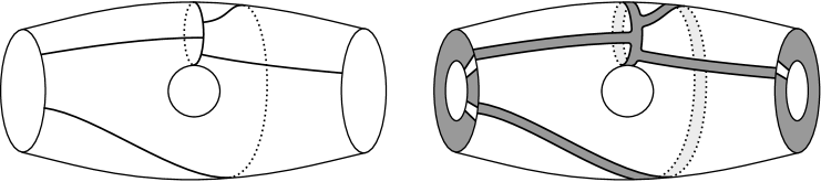
Figure 2. Left, an arc configuration on a genus one surface with two boundary components. Right, the thickened surface with the negative regions on $F\times\{1\}$ and $\partial F\times[-1,1]$ shaded.

Suppose the surface $F$ above is an auxiliary surface for $(M,\Gamma)$, and consider the preclosure $M^{\prime}=M\cup_{h}F\times[-1,1]$ associated to some neighborhood $A(\Gamma)$ and diffeomorphism

$$h:\partial F\times[-1,1]\rightarrow A(\Gamma).$$

We would like to define a contact structure $\xi^{\prime}$ on $M^{\prime}$ in terms of $\Xi_{\mathcal{A}}$ and $\xi$. To do so, we first perturb $\xi$ in a neighborhood of $A(\Gamma)$ so that $h$ identifies $\Xi_{\mathcal{A}}$ with this perturbed contact structure. This enables us to glue $F\times[-1,1]$ to $M$ via $h$ contact geometrically. We will show (Theorem 3.3) that the resulting contact preclosure $(M^{\prime},\xi^{\prime})$ is independent, up to flexibility and contactomorphism, of the arc configuration $\mathcal{A}$ and the other choices involved.

We start by describing the perturbation of $\xi$. Label the components of $\Gamma$ by $\Gamma_{1},\dots,\Gamma_{m}$. Each $\Gamma_{i}$ has an annular neighborhood $B_{i}\subset\partial M$ on which the leaves of the characteristic foliation are cocores with no singularities. Let $B(\Gamma)$ be the union of these $B_{i}$. Let $A_{i}$ be the component of $A(\Gamma)$ containing $\Gamma_{i}$. We will assume that $A_{i}\subset{\rm int}(B_{i})$. The map $h$ identifies $A_{i}$ with $\partial_{i}F\times[-1,1]$ for some component $\partial_{i}F$ of $\partial F$. In this way, the ordering on the components of $\Gamma$ induces an ordering on the components of $\partial F$. Let $k_{i}$ be the number of arcs in $\mathcal{A}$ with an endpoint on $\partial_{i}F$. The dividing set on the annulus $\partial_{i}F\times[-1,1]$ thus consists of $2k_{i}$ cocores.

The rough idea is to perturb $\xi$ to a contact structure $\xi_{h}$ whose dividing set $\Gamma_{h}$ restricts to $2k_{i}$ cocores of $A_{i}$, such that $h$ identifies the positive region of $\partial F\times[-1,1]$ with the negative region of $A(\Gamma)$ determined by $\Gamma_{h}$. We do essentially this, but work on the level of characteristic foliations rather than dividing curves for added control on the eventual contactomorphisms between different preclosures.

For $i=1,\dots,m$, let $C_{i}\subset{\rm int}(A_{i})$ be an annulus such that the intersection $\Gamma_{i}\cap C_{i}$ consists of $2k_{i}$ cocores of $C_{i}$. We next choose an isotopy

$$\varphi_{r}:\partial M\rightarrow\partial M,\,r\in[0,1]$$

which “straightens out” these $C_{i}$. Precisely, we require that $\varphi_{0}={id}$, that $\varphi_{1}(C_{i})=A_{i}$, that $h$ identifies the positive region of $\partial F\times[-1,1]$ with the negative region of $A(\Gamma)$ determined by the dividing set $\varphi_{1}(\Gamma)$, and that each $\varphi_{r}$ restricts to the identity outside of $B(\Gamma)$.

2pt$\Gamma_{i}$ at 44 38.5 $\varphi_{1}(\Gamma_{i})$ at 184 119 $C_{i}$ at 77 122 $\varphi_{1}(C_{i})=A_{i}$ at 210 -5 $B_{i}$ at 58 -5

Figure 3. Left, a view of $C_{i}\subset B_{i}$, where $k_{i}=3$. Right, $\varphi(\Gamma_{i})=\varphi_{1}(\Gamma_{i})$ and $\varphi_{1}(C_{i})=A_{i}$. The negative regions are shaded.

Choose a vertically invariant collar $\partial M\times(-\infty,0]$ of $\partial M=\partial M\times\{0\}$ such that $\Gamma$ is the dividing set associated to $\partial_{t}$. The isotopy $\varphi_{r}$ induces a diffeomorphism

$$\varphi:M\rightarrow M$$

as follows. Let

$$r:(-\infty,0]\rightarrow[0,1]$$

be a smooth function with

$$r(t)=\begin{cases}0&\text{for }t\leq-2\\ 1&\text{for }t\geq-1.\end{cases}$$

We define $\varphi$ to be the map defined by

(11) $$\varphi(x,t)=(\varphi_{r(t)}(x),t)$$

for $(x,t)\in\partial M\times(-\infty,0]$ and by the identity outside of $\partial M\times(-\infty,0]$. Note that $\varphi$ restricts to $\varphi_{1}$ on $\partial M$ and to the identity outside of $B(\Gamma)\times[-2,0]$.

Define $\xi_{0}:=\varphi_{*}(\xi)$. Let $\mathfrak{F}_{1}$ be a foliation of $\partial M$ divided by $\varphi(\Gamma)=\varphi_{1}(\Gamma)$ which agrees with $h(\partial F\times[-1,1])_{\Xi_{\mathcal{A}}}$ on $A(\Gamma)$ and with $\mathfrak{F}_{0}=(\partial M)_{\xi_{0}}$ outside of $B(\Gamma)$, as illustrated in Figure 4. We apply flexibility, as in Proposition 2.28, with respect to the collar determined by the contact vector field $\varphi_{*}(\partial_{t})$ for $\xi_{0}$, to obtain a contact structure $\xi_{1}=f_{01}(\xi_{0})$ with $(\partial M)_{\xi_{1}}=\mathfrak{F}_{1}$. In doing so, we can arrange that $\xi_{1}=h_{*}(\Xi_{\mathcal{A}})$ on $A(\Gamma)$, by Remark 2.29. Since $\mathfrak{F}_{0}$ and $\mathfrak{F}_{1}$ agree outside of $B(\Gamma)$, we can assume that $\partial_{t}$ is a contact vector field for $\xi_{01}$ on the complement of $B(\Gamma)\times[0,1]$ in the product $\partial M\times[0,1]$ used to define the map $f_{01}$. It then follows from the construction of $f_{01}$ that $\xi_{1}=\xi$ outside of $B(\Gamma)\times[-3,0]$, since $\xi_{0}$ and $\varphi_{*}(\partial_{t})$ agree with $\xi$ and $\partial_{t}$, respectively, outside of $B(\Gamma)\times[-2,0]$. We will hereafter denote $\xi_{1}$ by $\xi_{h}$ to indicate its dependence on $h$. We may now glue $(F\times[-1,1],\Xi_{\mathcal{A}})$ to $(M,\xi_{h})$ via $h$ contact geometrically. We perform this gluing, rounding corners as illustrated in Figure 5, to obtain a contact preclosure

$$(M^{\prime},\xi^{\prime})=(M\cup_{h}F\times[-1,1],\xi_{h}\cup\Xi_{\mathcal{A}})$$

of $(M,\Gamma,\xi)$.

Remark 3.2.

The dividing set for $\xi^{\prime}$ consists of two parallel nonseparating curves on each component $\partial_{\pm}M^{\prime}$ of $\partial M^{\prime}$. The negative region on $\partial_{+}M^{\prime}$ is the annulus bounded by these curves and retracts onto a regular neighborhood of $c\times\{1\}$, where $c$ is the curve in $\mathcal{A}$. Likewise, the positive region on $\partial_{-}M^{\prime}$ is an annulus which retracts onto a neighborhood of $c\times\{-1\}$.

Figure 4. Left, a view of $A_{i}$, $B_{i}$, and $\varphi(\Gamma_{i})=\varphi_{1}(\Gamma_{i})$. Right, a view of the foliation $\mathfrak{F}_{1}$ in the portion of $B_{i}$ contained within the dotted rectangle.

2pt

$h$ at 108 13 $h$ at 108 155

Figure 5. Left, gluing $\partial F\times[-1,1]$ to $M$ along $A(\Gamma)$, as viewed near some $B_{i}\times(-\infty,0]$. Middle, the glued manifold. Right, the contact preclosure with convex boundary after rounding corners.

The rest of this subsection is devoted to proving the well-definedness of $(M^{\prime},\xi^{\prime})$. Our main result is the following.

Theorem 3.3.

Suppose $(M^{\prime}_{1},\xi^{\prime}_{1})$ and $(M^{\prime}_{2},\xi^{\prime}_{2})$ are contact preclosures of $(M,\Gamma,\xi)$ defined using auxiliary surfaces of the same genus. Then, up to flexibility, $(M_{1}^{\prime},\xi_{1}^{\prime})$ and $(M_{2}^{\prime},\xi_{2}^{\prime})$ are contactomorphic by a map isotopic to one that restricts to the identity on $M\smallsetminus N(\Gamma)$ for some regular neighborhood $N(\Gamma)$ of $\Gamma$.

Proof.

First, suppose all choices in the constructions of $(M^{\prime}_{1},\xi^{\prime}_{1})$ and $(M^{\prime}_{2},\xi^{\prime}_{2})$ are the same except for that of the vertically invariant collar of $\partial M$ used to define $\xi_{h}$. Suppose $\xi_{h,1}$ and $\xi_{h,2}$ are the contact structures on $M$ defined from two different collars. The connectedness of the space of such collars implies that $\xi_{h,1}$ and $\xi_{h,2}$ are isotopic by an isotopy stationary on $\partial M$. It follows that $(M^{\prime}_{1},\xi^{\prime}_{1})$ and $(M^{\prime}_{2},\xi^{\prime}_{2})$ are contactomorphic by a map isotopic to one that restricts to the identity on $M$, as desired. It therefore suffices to prove Theorem 3.3 in the case that $(M^{\prime}_{1},\xi^{\prime}_{1})$ and $(M^{\prime}_{2},\xi^{\prime}_{2})$ are defined using the same collar. We will assume below that this is the case. We will also continue to think of the contact structure $\Xi_{\mathcal{A}}$ as being completely determined by the arc configuration $\mathcal{A}$. This is fine for the purpose of this proof: since any two such $\Xi_{\mathcal{A}}$ are related by flexibility and isotopy as in Lemma 2.35 and Remark 2.36, the contact preclosures formed from any two such $\Xi_{\mathcal{A}}$ are related as claimed in the theorem, assuming all other choices are the same.

Below, we prove Theorem 3.3 in the case that $(M^{\prime}_{1},\xi^{\prime}_{1})$ and $(M^{\prime}_{2},\xi^{\prime}_{2})$ are built using auxiliary surfaces with isomorphic arc configurations.

Definition 3.4.

Suppose $\mathcal{A}_{1}$ and $\mathcal{A}_{2}$ are arc configurations on $F_{1}$ and $F_{2}$, and suppose the boundary components of each $F_{j}$ have been ordered. We say that $\mathcal{A}_{1}$ and $\mathcal{A}_{2}$ are isomorphic if there is a diffeomorphism from $(F_{1},\mathcal{A}_{1})$ to $(F_{2},\mathcal{A}_{2})$ which respects these boundary orderings.

For $k=1,2$, suppose $(M^{\prime}_{k},\xi^{\prime}_{k})$ is defined using the auxiliary surface $F_{k}$, the arc configuration $\mathcal{A}_{k}$, the neighborhoods $A(\Gamma)_{k}=\cup_{i}A_{i,k}$ and $B(\Gamma)_{k}=\cup_{i}B_{i,k}$, and the diffeomorphism $h_{k}$. For $i=1,\dots,m$, let $B_{i}$ be an annular neighborhood of $\Gamma_{i}$ containing $B_{i,1}\cup B_{i,2}$ on which the leaves of $(\partial M)_{\xi}$ are cocores with no singularities, and let $B(\Gamma)=\cup_{i}B_{i}$. Let us assume that $\mathcal{A}_{1}$ and $\mathcal{A}_{2}$ are isomorphic (where the boundary components of $F_{k}$ are ordered according to $h_{k}$ and the ordering of the components of $\Gamma$, as usual) by an isomorphism

$$g:(F_{1},\mathcal{A}_{1})\to(F_{2},\mathcal{A}_{2}).$$

Note that $g$ induces a canonical isotopy class of contactomorphisms

$$\tilde{g}:(F_{1}\times[-1,1],\Xi_{\mathcal{A}_{1}})\to(F_{2}\times[-1,1],\Xi_{\mathcal{A}_{2}})$$

for which $h_{2}\circ\tilde{g}\circ h_{1}^{-1}$ restricts to a diffeomorphism from $A_{i,1}$ to $A_{i,2}$ for $i=1,\dots,m$. Let

$$\varphi_{r}:\partial M\rightarrow\partial M,\,r\in[0,1],$$

be an isotopy supported in $B(\Gamma)$, such that $\varphi_{0}={id}$ and $\varphi_{1}$ restricts to the map

$$h_{2}\circ\tilde{g}\circ h_{1}^{-1}:A(\Gamma)_{1}\rightarrow A(\Gamma)_{2}.$$

Let

$$\varphi:M\to M$$

be the diffeomorphism of $M$ extending $\varphi_{1}$ defined as in (11). By construction, the characteristic foliations of $\xi_{h_{1}}$ and $(\varphi_{*})^{-1}(\xi_{h_{2}})$ on $\partial M$ agree on $A(\Gamma)_{1}$ and outside of $B(\Gamma)$. Let $\xi_{h_{1}}^{\prime}$ be a contact structure obtained from $\xi_{h_{1}}$ by flexibility such that

$$(\partial M)_{\xi_{h_{1}}^{\prime}}=(\partial M)_{(\varphi_{*})^{-1}(\xi_{h_{2}})}$$

and such that $\xi_{h_{1}}^{\prime}$ agrees with $\xi_{h_{1}}$ on $A(\Gamma)_{1}\times[-3,0]$ and outside of $B(\Gamma)\times[-3,0]$. The contact preclosure $(M_{1}^{\prime},\xi_{1}^{\prime\prime})$ constructed from $\xi_{h_{1}}^{\prime}$ is then related to $(M_{1}^{\prime},\xi_{1}^{\prime})$ by flexibility.

To complete the proof of Theorem 3.3 in this case, it therefore suffices to show that $(M_{1}^{\prime},\xi_{1}^{\prime\prime})$ is contactomorphic to $(M_{2}^{\prime},\xi_{2}^{\prime})$ by a map isotopic to one that restricts to the identity outside of $B(\Gamma)\times[-3,0]$. For this, it suffices to show that $(M,\xi_{h_{1}}^{\prime})$ is contactomorphic to $(M,\xi_{h_{2}})$ by a map isotopic to one which restricts to the identity outside of $B(\Gamma)\times[-3,0]$, through maps which restrict to $h_{2}\circ\tilde{g}\circ h_{1}^{-1}$ on $A(\Gamma)_{1}$. Indeed, a contactomorphism from $(M,\xi_{h_{1}}^{\prime})$ to $(M,\xi_{h_{2}})$ of this form extends to the desired contactomorphism from $(M_{1}^{\prime},\xi_{1}^{\prime\prime})$ to $(M_{2}^{\prime},\xi_{2}^{\prime})$ by the map $\tilde{g}$. Since $(\varphi_{*})^{-1}(\xi_{h_{2}})$ is already contactomorphic to $\xi_{h_{2}}$ by such a map (namely, $\varphi$), it suffices to show that $\xi_{h_{1}}^{\prime}$ and $(\varphi_{*})^{-1}(\xi_{h_{2}})$ are isotopic by an isotopy stationary on $\partial M$. To see this, let $d_{i}$ be one of the boundary components of $B_{i}$. For each $t$, the multicurve $\cup_{i}\,(d_{i}\times\{t\})$ divides the characteristic foliations on $\partial M\times\{t\}$ induced by $\xi_{h_{1}}^{\prime}$ and $(\varphi_{*})^{-1}(\xi_{h_{2}})$. Since these two contact structures induce the same characteristic foliations on $\partial M$ and agree outside of $\partial M\times[-3,0]$, Lemma 2.26 implies that $\xi_{h_{1}}^{\prime}$ and $(\varphi_{*})^{-1}(\xi_{h_{2}})$ are isotopic by an isotopy stationary on $\partial M$ (and outside of $\partial M\times[-3,0]$), as desired.

It remains to prove Theorem 3.3 in the case that $(M^{\prime}_{1},\xi^{\prime}_{1})$ and $(M^{\prime}_{2},\xi^{\prime}_{2})$ are defined using auxiliary surfaces of the same genus with nonisomorphic arc configurations. For this, we will need a way of relating nonisomorphic configurations.

Definition 3.5.

Suppose $\mathcal{A}=\{c,a_{1},\dots,a_{m}\}$ is an arc configuration on a surface $F$ with ordered boundary components $\partial_{1}F,\dots,\partial_{m}F$, and suppose the arcs have been labeled so that $a_{i}$ is the (unique) arc meeting $\partial_{i}F$. Suppose further that when $c$ is traversed according to one of its two orientations, the arcs $a_{1},\dots,a_{m}$ appear “locally” to the left of $c$ and in that cyclic order, as depicted in Figure 6. Such an arc configuration is called standard.

2pt$c$ at -7 52 $a_{1}$ at 25 78 $a_{2}$ at 53 72 $a_{3}$ at 83 70 $a_{m}$ at 135 77

Figure 6. A standard arc configuration in a neighborhood of $c$.

Lemma 3.6.

If $\mathcal{A}_{1}$ and $\mathcal{A}_{2}$ are standard arc configurations on surfaces $F_{1}$ and $F_{2}$ of the same genus and with the same number of boundary components, then $\mathcal{A}_{1}$ and $\mathcal{A}_{2}$ are isomorphic.

Proof.

For $k=1,2$, let $F_{k}^{\prime}$ be the surface obtained by cutting $F_{k}$ open along the curve and arcs in $\mathcal{A}_{k}$. The first condition in Definition 3.5 implies that $F_{1}^{\prime}$ and $F_{2}^{\prime}$ have the same genus and two boundary components. Moreover, one boundary component of $F^{\prime}_{k}$ is partitioned into segments labeled by elements of $\mathcal{A}_{k}$ and boundary components of $F_{k}$; the other is labeled solely by the curve in $\mathcal{A}_{k}$. The second condition in Definition 3.5 implies that there is an orientation-preserving homeomorphism from $F_{1}^{\prime}$ to $F_{2}^{\prime}$ which preserves this labeling (with respect to the natural bijections between elements of $\mathcal{A}_{1}$ and $\mathcal{A}_{2}$ and between components of $\partial F_{1}$ and $\partial F_{2}$). The lemma follows. ∎

We now define two “moves” on arc configurations: addition is the process of adding one arc to a configuration while deletion is the process of deleting arcs from a configuration until there is exactly one arc meeting each boundary component. It is easy to see that one can transform any arc configuration into a standard one via a finite sequence of these moves: one first uses deletion to obtain a configuration in which there is exactly one arc meeting each boundary component and then alternates additions with deletions to turn this configuration into a standard one, as illustrated in Figure 7. It follows that arbitrary arc configurations on surfaces of the same genus and with the same number of boundary components can be made isomorphic after finitely many additions and deletions. Thus, to complete the proof of Theorem 3.3, it suffices to show that the theorem holds for contact preclosures built from arc configurations related by deletion (for an arc configuration with exactly one arc meeting each boundary component, an addition is the inverse of a deletion).

2pt $1$ at 28 -9 $2$ at 28 140 $3$ at 111 140 $4$ at 111 -9

Figure 7. Making an arc configuration standard through an alternating sequence of additions and deletions. The four boundary components are labeled as shown on the left.

Fix an auxiliary surface $F$, the neighborhoods $A(\Gamma)$ and $B(\Gamma)$, and the diffeomorphism $h$. Let $\mathcal{A}_{1}$ be an arbitrary arc configuration on $F$ and suppose $\mathcal{A}_{2}$ is obtained from $\mathcal{A}_{1}$ by deletion. The dividing set $\Gamma_{\mathcal{A}_{2}}$ is normally defined in terms of the boundary of a regular neighborhood of $\mathcal{A}_{2}$, as in (10). Below, we will instead imagine $\Gamma_{\mathcal{A}_{2}}$ as coming from the boundary of a regular neighborhood of a certain graph $\mathcal{A}_{1}^{\prime}$ on $F$,

$$\Gamma_{\mathcal{A}_{2}}=-\overline{(\partial N(\mathcal{A}_{1}^{\prime})\smallsetminus\partial M)}.$$

This graph $\mathcal{A}^{\prime}_{1}$ is obtained by retracting arcs of $\mathcal{A}_{1}$ a short distance into $F$ until there is exactly one arc meeting each boundary component, as shown in Figure 8. We retract precisely those arcs that are deleted when forming $\mathcal{A}_{2}$ from $\mathcal{A}_{1}$. Although $\mathcal{A}_{1}^{\prime}$ is not an arc configuration in general, a neighborhood of this graph retracts onto a neighborhood of $\mathcal{A}_{2}$, so these two ways of defining $\Gamma_{\mathcal{A}_{2}}$ result in isotopic dividing sets.

Below, we will use the notation $\xi_{h,k}$ in place of $\xi_{h}$ to denote the contact structure on $M$ defined using the map $h$ and the arc configuration $\mathcal{A}_{k}$. Our goal is to prove Theorem 3.3 for the contact preclosures

(12) $$(M_{1}^{\prime},\xi_{1}^{\prime}) =(M\cup_{h}F\times[-1,1],\xi_{h,1}\cup\Xi_{\mathcal{A}_{1}})$$

(13) $$(M_{2}^{\prime},\xi_{2}^{\prime}) =(M\cup_{h}F\times[-1,1],\xi_{h,2}\cup\Xi_{\mathcal{A}_{2}}).$$

We start by specifying the data needed to define the contact structures $\xi_{h,j}$. As usual, we will assume that the dividing set of $\Xi_{\mathcal{A}_{1}}$ on the annulus $\partial_{i}F\times[-1,1]$ consists of $2k_{i}$ cocores. Note that the dividing set of $\Xi_{\mathcal{A}_{2}}$ on each $\partial_{i}F\times[-1,1]$ consists of just $2$ cocores.

2pt

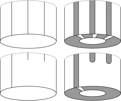
Figure 8. Top: left, the arc configuration $\mathcal{A}_{1}$ near a component $\partial_{i}F$; right, the corresponding portion of $(F\times[-1,1],\Xi_{\mathcal{A}_{1}})$. Bottom: left, the graph $\mathcal{A}^{\prime}_{1}$ obtained from $\mathcal{A}_{1}$ by retracting all but one of the arcs meeting each boundary component of $F$; right, the corresponding portion of $(F\times[-1,1],\Xi_{\mathcal{A}_{2}})$.

For $i=1,\dots,m$, let $D_{i}\subset{\rm int}(A_{i})$ be an annulus which intersects $\Gamma_{i}$ in $2$ cocores, and let $D(\Gamma)=\bigcup_{i}D_{i}$. Let $C_{i,1}\subset{\rm int}(D_{i})$ be an annulus which intersects $\Gamma_{i}$ in $2k_{i}$ cocores. In particular, we require that one component of $D_{i}\cap\Gamma_{i}$ intersects $C_{i,1}$ in $1$ cocore while the other intersects $C_{i,1}$ in $2k_{i}-1$ cocores. Finally, let $C_{i,2}\subset{\rm int}(D_{i})$ be an annulus which intersects $\Gamma_{i}$ in $2$ cocores. See Figure 9 for an illustration of these annuli after straightening below. The annuli $C_{i,1}$ and $C_{i,2}$ will be used to define the contact structures $\xi_{h,1}$ and $\xi_{h,2}$ in the usual way while the $D_{i}$ are auxiliary annuli that will be used to relate $(M_{1}^{\prime},\xi_{1}^{\prime})$ and $(M_{2}^{\prime},\xi_{2}^{\prime})$.

2pt$\phi_{2}(D_{i})$ at 219 122 $\phi_{2}(C_{i,2})$ at 218 -6 $\phi_{1}(D_{i})$ at 68 122 $\phi_{1}(C_{i,1})$ at 67 -6 $\phi_{1}(\Gamma_{i})$ at 15 68 $\phi_{2}(\Gamma_{i})$ at 166 68

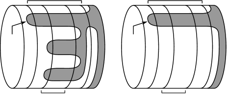
Figure 9. A view from within $B_{i}$ of the annuli $D_{i}$, $C_{i,1}$, and $C_{i,2}$ after straightening by $\varphi_{1}$ on the left and $\varphi_{2}$ on the right. In particular, $\varphi_{1}(C_{i,1})=\varphi_{2}(C_{i,2})=A_{i}$ and $\varphi_{1}(D_{i})=\varphi_{2}(D_{i})$.

Let $\mathfrak{F}$ be a foliation of $\partial M$ divided by $\Gamma$ which contains the boundary components $d_{i}^{\pm}$ of $D_{i}$ as unions of leaves and agrees with $(\partial M)_{\xi}$ outside of $B(\Gamma)$. Let $\xi^{\prime}$ be the contact structure with $(\partial M)_{\xi^{\prime}}=\mathfrak{F}$ obtained from $\xi$ by flexibility. Note that the curves $d_{i}^{\pm}$ are Legendrian with respect to $\xi^{\prime}$. Choose a vertically invariant collar $\partial M\times(-\infty,0]$ of $\partial M$ with respect to $\xi^{\prime}$. We can arrange (by choosing $\mathfrak{F}$ more carefully) that $\xi^{\prime}$ is invariant in the $[-\epsilon,\epsilon]$-direction for some small tubular neighborhoods $d_{i}^{\pm}\times[-\epsilon,\epsilon]\subset\partial M$ of the $d_{i}^{\pm}=d_{i}^{\pm}\times\{0\}$. This implies that the annuli (with corners) given by

$$E_{i}=(d_{i}^{+}\times[-4,0]_{t})\,\cup\,(D_{i}\times\{-4\}_{t})\,\cup(d_{i}^{-}\times[-4,0]_{t})\,\subset\,\partial M\times(-\infty,0]_{t}$$

are convex.

We now construct the isotopies of $\partial M$ which “straighten out” the annuli $C_{i,1}$ and $C_{i,2}$. For $k=1,2$, let

$$\varphi_{r,k}:\partial M\rightarrow\partial M,\,r\in[0,1],$$

be an isotopy supported in $B(\Gamma)$ such that $\varphi_{0,k}={id}$, $\varphi_{1,k}(C_{i,k})=A_{i}$, and $h$ identifies the positive region on $\partial_{i}F\times[-1,1]$ with respect to $\Xi_{\mathcal{A}_{k}}$ with the negative region on $A_{i}$ determined by $\varphi_{1,k}(\Gamma)$. We will additionally require that $\varphi_{r,1}=\varphi_{r,2}$ in a neighborhood of the curves $d_{i}^{\pm}$ and outside $D(\Gamma)$. Let

$$\varphi_{k}:M\to M$$

be the diffeomorphism of $M$ extending $\varphi_{1,k}$ defined as in (11)), and define $\xi_{0,k}:=(\varphi_{k})_{*}(\xi^{\prime})$. Note that $\xi_{0,1}=\xi_{0,2}$ outside of

(14) $$\varphi_{1}(D(\Gamma)\times[-3,0])=\varphi_{2}(D(\Gamma)\times[-3,0])$$

and in neighborhoods of the annuli $G_{i}=\varphi_{1}(E_{i})=\varphi_{2}(E_{i}).$

For $k=1,2$, let $\mathfrak{F}_{1,k}$ be a foliation of $\partial M$ divided by $\varphi_{k}(\Gamma)$ which agrees on $A(\Gamma)$ with the image of the characteristic foliation $(\partial F\times[-1,1])_{\Xi_{\mathcal{A}_{k}}}$ under $h$ and with $\mathfrak{F}_{0,k}:=(\partial M)_{\xi_{0,k}}$ outside of $B(\Gamma)$. We will additionally require that $\mathfrak{F}_{1,1}$ and $\mathfrak{F}_{1,2}$ agree outside of $\varphi_{1}(D(\Gamma))=\varphi_{2}(D(\Gamma)).$ Let $\xi_{1,k}$ be the contact structure with $(\partial M)_{\xi_{1,k}}=\mathfrak{F}_{1,k}$ obtained from $\xi_{0,k}$ by flexibility, using the collar determined by the contact vector field $(\varphi_{k})_{*}(\partial_{t})$ for $\xi_{0,k}$. As usual, we let $\xi_{h,k}:=\xi_{1,k}$. We can arrange that the annuli $G_{i}$ are convex for both $\xi_{h,1}$ and $\xi_{h,2}$ and, moreover, that $\xi_{h,1}$ and $\xi_{h,2}$ agree in neighborhoods of these annuli and outside the neighborhood of $\Gamma$ in (14). Let $N(\Gamma)$ denote the component of $M\smallsetminus\cup_{i}G_{i}$ containing $\Gamma$. Then, in particular, $\xi_{h,1}=\xi_{h,2}$ on $M\smallsetminus N(\Gamma).$ We will record this fact as

(15) $$(M\smallsetminus N(\Gamma),\xi_{h,1})=(M\smallsetminus N(\Gamma),\xi_{h,2})$$

for later use.

We now prove Theorem 3.3 for the contact preclosures $(M_{1}^{\prime},\xi_{1}^{\prime})$ and $(M_{2}^{\prime},\xi_{2}^{\prime})$ formed from $\xi_{h,1}$ and $\xi_{h,2}$ as in (12) and (13). Since the convex surfaces

$$F\times\{t\}\subset(F\times[-1,1],\Xi_{\mathcal{A}_{1}})$$

have collared Legendrian boundary, there is a collar $\partial F\times[0,1]\subset F$ such that $\Xi_{\mathcal{A}_{1}}$ is invariant in the $[0,1]$-direction on

$$\partial F\times[0,1]\times[-1,1]\subset F\times[-1,1].$$

We can arrange that $\Xi_{\mathcal{A}_{2}}$ is invariant in the same direction on the smaller neighborhood

$$\partial F\times[0,1/2]\times[-1,1]\subset F\times[-1,1],$$

and that

(16) $$((F\smallsetminus(\partial F\times[0,1]))\times[-1,1],\Xi_{\mathcal{A}_{1}})=((F\smallsetminus(\partial F\times[0,1]))\times[-1,1],\Xi_{\mathcal{A}_{2}}).$$

Note that the annuli

$$H_{i}=\partial_{i}F\times\{1\}\times[-1,1]\,\,\,\,\,\,{\rm and}\,\,\,\,\,\,H_{i}^{\prime}=\partial_{i}F\times\{1/2\}\times[-1,1]$$

are convex with collared Legendrian boundary with respect to both $\Xi_{\mathcal{A}_{1}}$ and $\Xi_{\mathcal{A}_{2}}$. See Figure 10 for an illustration of these annuli.

2pt

$0$ at -5 20 $\frac{1}{2}$ at -5 67 $1$ at -5 114

$H_{i}^{\prime}$ at 193 91 $H_{i}$ at 193 136

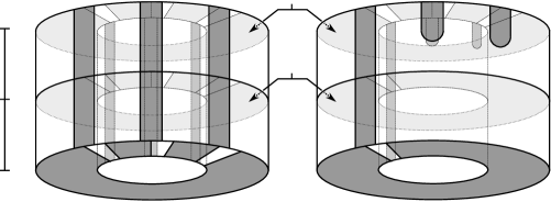
Figure 10. Left and right, the regions $\partial F\times[0,1]\times[-1,1]$ in $\Xi_{\mathcal{A}_{1}}$ and $\Xi_{\mathcal{A}_{2}}.$

For $k=1,2$, the annuli $G_{i}$ and $H_{i}$, together with two annuli in $\partial M_{k}^{\prime}$, bound a solid torus $T_{i,k}$ in $M_{k}^{\prime}$, as shown in Figure 11. Moreover, the complement $(M_{k}^{\prime}\smallsetminus\cup_{i}T_{i,k},\xi_{k}^{\prime})$ is the union of the pieces in (15) and (16), which implies that

$$(M_{1}^{\prime}\smallsetminus\cup_{i}T_{i,1},\xi_{1}^{\prime})=(M_{2}^{\prime}\smallsetminus\cup_{i}T_{i,2},\xi_{2}^{\prime}).$$

To prove Theorem 3.3, it therefore suffices to show that, after rounding corners, $(T_{i,1},\xi_{1}^{\prime})$ is contactomorphic to $(T_{i,2},\xi_{2}^{\prime})$, up to flexibility. But after rounding corners, $T_{i,1}$ and $T_{i,2}$ are solid tori with convex boundaries with dividing sets consisting of two parallel curves of slope $-1$, as shown in Figure 12 for $T_{i,2}$. As there is a unique tight solid torus with these boundary conditions, up to flexibility and contactomorphism, all that remains is to show that $(T_{i,1},\xi_{1}^{\prime})$ and $(T_{i,2},\xi_{2}^{\prime})$ are tight.

2pt $0$ at -8 403 $-\infty$ at -20 353 $H_{i}$ at 498 391 $G_{i}$ at 462 230 $T_{i,1}$ at 460 330 $T_{i,2}$ at 460 77

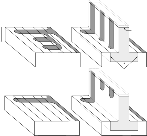
Figure 11. Top: left, $(M,\xi_{h,1})$ on a portion of $B_{i}\times(-\infty,0]$; right, the corresponding portion of $(M^{\prime},\xi_{1}^{\prime})$ gotten by attaching $(F\times[-1,1],\Xi_{\mathcal{A}_{1}})$. Bottom, the analogous pictures for $(M,\xi_{h,2})$ and $(M^{\prime},\xi_{2}^{\prime})$. The lightly shaded regions on the top and bottom are meridional disks for the tori $T_{i,1}$ and $T_{i,2}$.

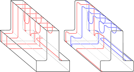
Figure 12. Left, the dividing set on $\partial T_{i,2}$. Right, the dividing set after rounding corners; it consists of two curves of slope $-1$ drawn in red and blue.

Lemma 3.7.

For $k=1,2$, the solid torus $(T_{i,k},\xi_{k}^{\prime})$ is tight.

Proof.

For $k=1$, this follows from the fact that $(T_{i,1},\xi_{1}^{\prime})$ can be embedded as a contact submanifold of some vertically invariant neighborhood of $B_{i}$ in which the characteristic foliation on each copy of $B_{i}$ agrees with that of $\xi_{h,1}$. To see that such a neighborhood is tight, note that it is related by flexibility to a vertically invariant neighborhood of $B_{i}$ in which the characteristic foliation on each copy of $B_{i}$ consists of cocores. The latter is, in some sense, a standard neighborhood of a dividing curve: it embeds as a neighborhood of any dividing curve on any convex surface in any contact manifold, and is therefore tight. The former neighborhood of $B_{i}$ is thus tight as well since flexibility preserves tightness. To see that $(T_{i,1},\xi_{1}^{\prime})$ embeds into such a neighborhood, note that $T_{i,1}$ is contained in a union

(17) $$(B_{i}\times(-\infty,0]_{s}\cup_{h}\partial F\times[0,1]_{s}\times[-1,1],\xi_{h,1}\cup\Xi_{\mathcal{A}_{1}}),$$

where $\xi_{h,1}$ on $B_{i}\times(-\infty,0]_{s}$ is invariant in the $\partial_{s}$-direction. Here, $\partial_{s}=(\varphi_{1})_{*}(\partial_{t}),$ where $\partial_{t}$ is the contact vector field for the vertically invariant collar $\partial M\times(-\infty,0]$ for $\xi^{\prime}$ discussed earlier. Since $\Xi_{\mathcal{A}_{1}}$ is invariant in the $[0,1]_{s}$-direction, the union in (17) can be embedded in a vertically invariant neighborhood $B_{i}\times(-\infty,1]_{s}$.

For $k=2$, let $T_{i,2}^{\prime}$ be the solid torus in $M_{2}^{\prime}$ bounded by $G_{i}$, $H_{i}^{\prime}$, and two annuli in $\partial M^{\prime}_{2}$. By the reasoning above (considering $\Xi_{\mathcal{A}_{2}}$ rather than $\Xi_{\mathcal{A}_{1}}$), the solid torus $(T_{i,2}^{\prime},\xi_{2}^{\prime})$ embeds into a vertically invariant neighborhood of $B_{i}$ and is therefore tight. Note that $(T_{i,2},\xi_{2}^{\prime})$ is obtained by gluing $(\partial_{i}F\times[1/2,1]\times[-1,1],\Xi_{\mathcal{A}_{2}})$ to $(T_{i,2}^{\prime},\xi_{2}^{\prime})$ along $H_{i}^{\prime}$. After rounding corners, the first piece is contactomorphic to the $[1/2,1]$-invariant contact structure specified by the dividing set of $\Xi_{\mathcal{A}_{2}}$ on $H_{i}^{\prime}$. Indeed, both are tight solid tori with convex boundaries and dividing sets consisting of two parallel curves of slope $-1$. It follows that $(T_{i,2},\xi_{2}^{\prime})$ is contactomorphic to the torus obtained from $(T_{i,2}^{\prime},\xi_{2}^{\prime})$ by attaching a vertically invariant neighborhood of some portion of $\partial T_{i,2}^{\prime}$. Thus, $(T_{i,2},\xi_{2}^{\prime})$ is contactomorphic to $(T_{i,2}^{\prime},\xi_{2}^{\prime})$, and, hence, tight. ∎

This concludes the proof of Theorem 3.3. ∎

The corollary below follows easily from the proof of Theorem 3.3.

Corollary 3.8.

Suppose $(M,\Gamma,\xi_{1})$ and $(M,\Gamma,\xi_{2})$ are related by flexibility, with contact preclosures $(M^{\prime}_{1},\xi^{\prime}_{1})$ and $(M^{\prime}_{2},\xi^{\prime}_{2})$ defined using auxiliary surfaces of the same genus. Then, up to flexibility, $(M_{1}^{\prime},\xi_{1}^{\prime})$ and $(M_{2}^{\prime},\xi_{2}^{\prime})$ are contactomorphic by a map smoothly isotopic to one that restricts to the identity on $M\smallsetminus N(\Gamma)$ for some regular neighborhood $N(\Gamma)$ of $\Gamma$. ∎

3.2. Contact closures and the invariants $\psi^{g}(M,\Gamma,\xi)$ and $\psi(M,\Gamma,\xi)$

Suppose $(M^{\prime},\xi^{\prime})$ is a contact preclosure of $(M,\Gamma,\xi)$. As mentioned in Remark 3.2, the dividing set for $\xi^{\prime}$ consists of two parallel nonseparating curves on each component $\partial_{\pm}M^{\prime}$ of $\partial M^{\prime}$. One can therefore glue $\partial_{+}M^{\prime}$ to $\partial_{-}M^{\prime}$ (after applying flexibility, of course) by a map which identifies the positive region on $\partial_{+}M^{\prime}$ with the negative region on $\partial_{-}M^{\prime}$ to form a closed contact manifold $(Y,\bar{\xi})$ with a distinguished convex surface $R:=\partial_{+}M^{\prime}=-\partial_{-}M^{\prime}$. We call a triple $(Y,R,\bar{\xi})$ formed in this way a simple contact closure of $(M,\Gamma,\xi)$. One might then attempt to define an invariant of $\xi$ in terms of the contact invariant $\psi(Y,\bar{\xi})$. We do essentially this but, for naturality purposes, need the following slightly more involved notion of contact closure.

Definition 3.9.

A contact closure of $(M,\Gamma,\xi)$ consists of a closure $\mathscr{D}=(Y,R,r,m)$ of $(M,\Gamma)$ together with a contact structure $\bar{\xi}$ on $Y$ such that

1. $m$ restricts to a contact embedding of $(M\smallsetminus N(\Gamma),\xi)$ into $(Y,\bar{\xi})$ for some regular neighborhood $N(\Gamma)$ of $\Gamma$,

2. this restriction of $m$ extends to a contactomorphism

   $$(M^{\prime},\xi^{\prime})\to(Y\smallsetminus{\rm int}({\rm Im}(r)),\bar{\xi})$$

   for some contact preclosure $(M^{\prime},\xi^{\prime})$ of $(M,\Gamma,\xi)$.

3. $r^{*}(\bar{\xi})$ is a contact structure on $R\times[-1,1]$ obtained, via flexibility, from one that is invariant in the $[-1,1]$-direction.

Remark 3.10.

Note that $(M,\Gamma,\xi)$ admits a genus $g$ contact closure for every $g\geq g(M,\Gamma)$.

Remark 3.11.

For a contact closure $(\mathscr{D},\bar{\xi})$ as in Definition 3.9, the triple $(Y,r(R\times\{t\}),\bar{\xi})$ is a simple contact closure of $(M,\Gamma,\xi)$ as described at the top for any $t\in[0,1]$. In particular, each $r(R\times\{t\})$ is convex with negative region an annulus bounded by essential curves.

Definition 3.12.

A marked contact closure of $(M,\Gamma,\xi)$ is a marked closure $\mathscr{D}=(Y,R,r,m,\eta)$ of $(M,\Gamma)$ together with a contact structure $\bar{\xi}$ on $Y$ such that $((Y,R,r,m),\bar{\xi})$ is a contact closure as in Definition 3.9 and $r(\eta\times\{0\})$ is dual to the core of the negative annular region of $r(R\times\{0\})$.

Suppose $(\mathscr{D}=(Y,R,r,m,\eta),\bar{\xi})$ is a marked contact closure of $(M,\Gamma,\xi)$ of genus $g$. Let $r(R\times\{0\})_{\pm}$ denote the positive and negative regions of $r(R\times\{0\})$. It is a standard result in convex surface theory that

$$\langle c_{1}(\mathfrak{s}_{\bar{\xi}}),r(R\times\{0\})\rangle_{Y}=\chi(r(R\times\{0\})_{+})-\chi(r(R\times\{0\})_{-}),$$

which is equal to $2-2g$ in this case since $r(R\times\{0\})_{-}$ is an annulus. It follows that

$$\langle c_{1}(\mathfrak{s}_{\bar{\xi}}),r(-R\times\{0\})\rangle_{-Y}=2g-2,$$

which implies that

$$\widecheck{\mathit{HM}}_{\bullet}(-Y,\mathfrak{s}_{\bar{\xi}};\Gamma_{-\eta})\subset\widecheck{\mathit{HM}}_{\bullet}(-Y|{-}R;\Gamma_{-\eta})=\underline{SHM}(-\mathscr{D}),$$

where $-\mathscr{D}$ is the corresponding marked closure of $(-M,-\Gamma)$. In particular,

$$\psi(Y,\bar{\xi})\in\underline{SHM}(-\mathscr{D}).$$

This leads to the following definition.

Definition 3.13.

Given a marked contact closure $(\mathscr{D}=(Y,R,r,m,\eta),\bar{\xi})$ of $(M,\Gamma,\xi)$ of genus $g\geq g(M,\Gamma)$, we define $\psi^{g}(M,\Gamma,\xi)$ to be the element of $\textbf{{\text@underline{SHM}}}(-M,-\Gamma)$ determined by the equivalence class of

$$\psi(\mathscr{D},\bar{\xi}):=\psi(Y,\bar{\xi})\in\underline{SHM}(-\mathscr{D}),$$

in the sense of Remark 2.8.

In Section 4, we will prove that $\psi^{g}(M,\Gamma,\xi)$ is well-defined for each $g$, per the following theorem.

Theorem 3.14.

If $(\mathscr{D},\bar{\xi})$ and $(\mathscr{D}^{\prime},\bar{\xi}^{\prime})$ are two marked contact closures of $(M,\Gamma,\xi)$ of the same genus, then

$$\underline{\Psi}_{-\mathscr{D},-\mathscr{D}^{\prime}}(\psi(\mathscr{D},\bar{\xi}))\doteq\psi(\mathscr{D}^{\prime},\bar{\xi}^{\prime}).$$

Furthermore, we will show that for $g$ sufficiently large, the contact elements $\psi^{g}(M,\Gamma,\xi)$ are equal, per the following theorem.

Theorem 3.15.

For every $(M,\Gamma,\xi)$, there is an integer $N(M,\Gamma,\xi)$ such that if $(\mathscr{D},\bar{\xi})$ and $(\mathscr{D}^{\prime},\bar{\xi}^{\prime})$ are marked contact closures of $(M,\Gamma,\xi)$ of genus at least $N(M,\Gamma,\xi)$, then

$$\underline{\Psi}_{-\mathscr{D},-\mathscr{D}^{\prime}}(\psi(\mathscr{D},\bar{\xi}))\doteq\psi(\mathscr{D}^{\prime},\bar{\xi}^{\prime}).$$

This theorem motivates the following definition.

Definition 3.16.

We define

$$\psi(M,\Gamma,\xi):=\psi^{g}(M,\Gamma,\xi)\in\textbf{{\text@underline{SHM}}}(-M,-\Gamma)$$

for any $g\geq N(M,\Gamma,\xi)$.

We will prove Theorems 3.14 and 3.15 in Section 4.

3.3. Properties

Below, we assume Theorems 3.14 and 3.15 hold in order to state and prove some basic properties about our contact invariants. We state these results for the invariants $\psi^{g}$. By Theorem 3.15, they also hold for the invariant $\psi$.

Lemma 3.17.

Suppose $f$ is a contactomorphism from $(M,\Gamma,\xi)$ to $(M^{\prime},\Gamma^{\prime},\xi^{\prime})$. Then the induced map

$$\textbf{{\text@underline{SHM}}}(f):\textbf{{\text@underline{SHM}}}(-M,-\Gamma)\to\textbf{{\text@underline{SHM}}}(-M^{\prime},-\Gamma^{\prime})$$

sends $\psi^{g}(M,\Gamma,\xi)$ to $\psi^{g}(M^{\prime},\Gamma^{\prime},\xi^{\prime})$.

Proof.

Essentially, a contactomorphism gives rise to contactomorphic closures. More precisely, suppose $(\mathscr{D}^{\prime},\bar{\xi}^{\prime})$ is a marked contact closure of $(M^{\prime},\Gamma^{\prime},\xi^{\prime})$. Since $f$ is a contactomorphism, $(\mathscr{D}^{\prime}_{f},\bar{\xi}^{\prime})$, as defined in (9), is a marked contact closure of $(M,\Gamma,\xi)$. According to the definition of $\textbf{{\text@underline{SHM}}}(f)$ in Subsection 2.2, it suffices to show that the identity map

$$id_{-\mathscr{D}^{\prime}_{f},-\mathscr{D}^{\prime}}:\underline{SHM}(-\mathscr{D}^{\prime}_{f})\to\underline{SHM}(-\mathscr{D}^{\prime})$$

sends $\psi(\mathscr{D}^{\prime}_{f},\bar{\xi}^{\prime})$ to $\psi(\mathscr{D}^{\prime},\bar{\xi}^{\prime})$. But this is immediate since

$$\psi(\mathscr{D}^{\prime}_{f},\bar{\xi}^{\prime})=\psi(Y^{\prime},\bar{\xi}^{\prime})=\psi(\mathscr{D}^{\prime},\bar{\xi}^{\prime}).\qed$$

Since the map $\textbf{{\text@underline{SHM}}}(f)$ only depends on the isotopy class of $f$, we have the following.

Corollary 3.18.

Suppose $(M,\Gamma,\xi)$ and $(M,\Gamma,\xi^{\prime})$ are sutured contact manifolds such that $\xi$ and $\xi^{\prime}$ are isotopic through diffeomorphisms fixing $\Gamma$. Then $\psi^{g}(M,\Gamma,\xi)=\psi^{g}(M,\Gamma,\xi^{\prime})$. ∎

The following corollary should be thought of as saying that $\psi^{g}(M,\Gamma,\xi)$ is essentially independent of the particular choice of multicurve $\Gamma$ dividing $(\partial M)_{\xi}$.

Corollary 3.19.

Suppose $(M,\Gamma,\xi)$ and $(M,\Gamma^{\prime},\xi)$ are sutured contact manifolds with the same underlying contact manifold but different dividing sets. Then there is a canonical isomorphism

$$\underline{\Psi}_{\xi,\Gamma,\Gamma^{\prime}}:\textbf{{\text@underline{SHM}}}(-M,-\Gamma)\to\textbf{{\text@underline{SHM}}}(-M,-\Gamma^{\prime})$$

sending $\psi^{g}(M,\Gamma,\xi)$ to $\psi^{g}(M,\Gamma^{\prime},\xi)$.

Proof.

Since the set of multicurves dividing $(\partial M)_{\xi}$ is connected, there is an isotopy

$$\varphi_{r}:\partial M\rightarrow\partial M,\,r\in[0,1],$$

such that $\varphi_{0}={id}$, each $\varphi_{r}$ preserves $(\partial M)_{\xi}$, and $\varphi_{1}(\Gamma_{i})=\Gamma_{i}^{\prime}$. Suppose $\partial M\times(-\infty,0]$ is a vertically invariant collar of $\partial M$, and extend $\varphi_{r}$ to a diffeomorphism

$$\varphi:M\to M$$

as in (11). It is easy to see, using Lemma 2.26, that $\xi$ and $\varphi_{*}(\xi)$ are isotopic by an isotopy stationary on $\partial M$. It then follows from Lemma 3.17 and Corollary 3.18 that

$$\underline{\Psi}_{\xi,\Gamma,\Gamma^{\prime}}:=\textbf{{\text@underline{SHM}}}(\varphi):\textbf{{\text@underline{SHM}}}(-M,-\Gamma)\to\textbf{{\text@underline{SHM}}}(-M,-\Gamma^{\prime})$$

sends $\psi^{g}(M,\Gamma,\xi)$ to $\psi^{g}(M,\Gamma^{\prime},\xi)$. That this isomorphism is “canonical” amounts to showing that it does not depend on the choices of $\varphi$ or the collar (that it is well-defined), and that

(18) $$\underline{\Psi}_{\xi,\Gamma,\Gamma^{\prime\prime}}=\underline{\Psi}_{\xi,\Gamma^{\prime},\Gamma^{\prime\prime}}\circ\underline{\Psi}_{\xi,\Gamma,\Gamma^{\prime}}$$

for any three multicurves $\Gamma,\Gamma^{\prime},\Gamma^{\prime\prime}$ dividing $(\partial M)_{\xi}$. The connectedness of the space of such collars implies that $\varphi$ is independent, up to isotopy stationary on $\partial M$, of the collar. Thus, $\textbf{{\text@underline{SHM}}}(\varphi)$ is independent of the collar. With that established, let us fix some collar, and suppose $\varphi^{1}$ and $\varphi^{2}$ are diffeomorphisms of $M$ as defined above. The contractibility of the space of multicurves dividing $(\partial M)_{\xi}$ implies that $\varphi^{1}$ and $\varphi^{2}$ are isotopic. It follows that

$$\textbf{{\text@underline{SHM}}}(\varphi^{1})=\textbf{{\text@underline{SHM}}}(\varphi^{2}).$$

Thus, $\underline{\Psi}_{\xi,\Gamma,\Gamma^{\prime}}$ is well-defined. Now, suppose $\varphi$ and $\varphi^{\prime}$ are diffeomorphisms of $M$ of the sort used to define the maps $\underline{\Psi}_{\xi,\Gamma,\Gamma^{\prime}}$ and $\underline{\Psi}_{\xi,\Gamma^{\prime},\Gamma^{\prime\prime}}$. The transitivity in (18) follows immediately from the fact that $\varphi^{\prime\prime}:=\varphi^{\prime}\circ\varphi$ is a diffeomorphism of the sort used to define $\underline{\Psi}_{\xi,\Gamma,\Gamma^{\prime\prime}}$. ∎

The corollary below indicates the invariance of $\psi^{g}$ with respect to flexibility.

Corollary 3.20.

Suppose $(M,\Gamma,\xi)$ and $(M,\Gamma,\xi^{\prime})$ are related by flexibility. Then $\psi^{g}(M,\Gamma,\xi)=\psi^{g}(M,\Gamma,\xi^{\prime})$.

Proof.

Suppose $(\mathscr{D}=(Y,R,r,m,\eta),\bar{\xi})$ is a marked contact closure of $(M,\Gamma,\xi)$. Corollary 3.8, together with Theorem 2.25, implies that $\bar{\xi}$ is isotopic to a contact structure $\bar{\xi}^{\prime}$ for which $(\mathscr{D},\bar{\xi}^{\prime})$ is a marked contact closure of $(M,\Gamma,\xi^{\prime})$. Then $\psi^{g}(M,\Gamma,\xi)=\psi^{g}(M,\Gamma,\xi^{\prime})$ since $\psi(\mathscr{D},\bar{\xi})=\psi(\mathscr{D},\bar{\xi}^{\prime})$. ∎

Remark 3.21.

The results above allow us to largely ignore, when dealing with the invariants $\psi^{g}$ and $\psi$, the differences between contact structures related by flexibility or isotopy. Accordingly, we will frequently work on the level of dividing sets rather than characteristic foliations and will often think of dividing sets as isotopy classes of multicurves.

Note if $(M,\Gamma,\xi)$ is overtwisted, then so is any contact closure $(\mathscr{D},\bar{\xi})$ of $(M,\Gamma,\xi)$. This implies that $\psi(\mathscr{D},\bar{\xi})=0$, by Theorem 2.20. The theorem below follows immediately.

Theorem 3.22.

If $(M,\Gamma,\xi)$ is overtwisted, then $\psi^{g}(M,\Gamma,\xi)=0$.∎

Given a closed contact 3-manifold $(Y,\xi)$, let $Y(p)$ denote the sutured contact manifold obtained from $Y$ by removing a Darboux ball centered at $p$. It is not hard to show that there is a canonical isotopy class of contactomorphisms relating any two such manifolds for a given point $p$, justifying our notation. When it is not important to keep track of $p$, we will write $Y(1)$ instead (as in the introduction), indicating that we have removed one Darboux ball. More generally, $Y(n)$ will refer to the (contactomorphism type of the) sutured contact manifold obtained by removing $n$ disjoint Darboux balls.

We will prove the following in Section 4.

Proposition 3.23.

There is a morphism

$$F_{p}:\textbf{{\text@underline{SHM}}}(-Y(p))\to\widecheck{\mathit{HM}}_{\bullet}(-Y)\otimes_{\mathbb{Z}}\mathcal{R}$$

which sends $\psi^{g}(Y(p))$ to $\psi(Y,\xi)\otimes\mathbf{1}$, where $\mathbf{1}$ refers to the equivalence class of $1\in\mathcal{R}$.

Since the monopole Floer invariant $\psi(Y,\xi)$ is nonzero for strongly symplectically fillable contact structures (see [20]), we have the following immediate corollary.

Corollary 3.24.

If $(Y,\xi)$ is strongly symplectically fillable, then $\psi^{g}(Y(p))\neq 0$. ∎

Remark 3.25.

The morphism in Proposition 3.23 can be thought of an analogue of the natural map in Heegaard Floer homology,

$$\widehat{HF}(-Y)\to HF^{+}(-Y),$$

which sends ${c}(Y,\xi)$ to $c^{+}(Y,\xi)$. Indeed, the modules comprising the systems $\textbf{{\text@underline{SHM}}}(-Y(p))$ and $\widecheck{\mathit{HM}}_{\bullet}(-Y)\otimes_{\mathbb{Z}}\mathcal{R}$ are isomorphic to $\widehat{HF}(-Y)\otimes_{\mathbb{Z}}\mathcal{R}$ and $HF^{+}(-Y)\otimes_{\mathbb{Z}}\mathcal{R}$, respectively.

Suppose $K$ is a Legendrian knot in the interior of $(M,\Gamma,\xi)$ and that $(M^{\prime},\Gamma^{\prime},\xi^{\prime})$ is the result of contact $(+1)$-surgery on $K$. We will prove the following in Section 4.

Proposition 3.26.

There is a morphism

$$F_{K}:\textbf{{\text@underline{SHM}}}(-M,-\Gamma)\to\textbf{{\text@underline{SHM}}}(-M^{\prime},-\Gamma^{\prime})$$

which sends $\psi^{g}(M,\Gamma,\xi)$ to $\psi^{g}(M^{\prime},\Gamma^{\prime},\xi^{\prime})$.

3.4. Examples

Below, we compute the contact invariants of the Darboux ball and product sutured contact handlebodies more generally. As above, we state these results in terms of the invariants $\psi^{g}$, but they also hold for the invariant $\psi$ by Theorem 3.15.

We start by constructing a genus $g$ marked contact closure of the Darboux ball $(B^{3},S^{1},\xi_{std})$ for each

$$g\geq g(B^{3},S^{1})=2$$

(where the dividing set $S^{1}$ is a single equatorial curve on $\partial B^{3}$). Consider the $[-1,1]$-invariant contact structure $\xi_{D^{2}}$ on $D^{2}\times[-1,1]$ for which each $D^{2}\times\{t\}$ is convex with collared Legendrian boundary and the dividing set on $D^{2}\times\{1\}$ consists of a single properly embedded arc, as shown in Figure 13. The product sutured contact manifold $(D^{2}\times[-1,1],\partial D^{2}\times\{0\},\xi_{D^{2}})$ is contactomorphic to $(B^{3},S^{1},\xi_{std})$ after rounding corners. One advantage of thinking of the Darboux ball in this way is that, in doing so, we have, in effect, automatically perturbed $\xi_{std}$ as required for forming contact preclosures.

2pt $\partial D^{2}\times\{0\}$ at -34 19 $S^{1}$ at 334 82

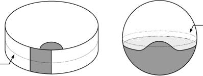
Figure 13. Left, $(D^{2}\times[-1,1],\xi_{D^{2}})$ with the negative region shaded. Right, the Darboux ball obtained by rounding corners.

Indeed, let $F$ be a genus $g\geq 2$ surface with one boundary component, and let $\mathcal{A}=\{c,a\}$ be an arc configuration on $F$ with a single arc. We may form a contact preclosure of the Darboux ball by gluing $(F\times[-1,1],\Xi_{\mathcal{A}})$ to $(D^{2}\times[-1,1],\xi_{D^{2}})$ according to a map

$$h:\partial F\times[-1,1]\to\partial D^{2}\times[-1,1]$$

of the form $f\times{\rm id}$ for some diffeomorphism $f:\partial F\to\partial D^{2}$, as in Figure 14. The result is a $[-1,1]$-invariant contact structure $\xi^{\prime}$ on $M^{\prime}=(D^{2}\cup F)\times[-1,1]$. Each $(D^{2}\cup F)\times\{t\}$ is convex with negative region an annular neighborhood $A(c)\times\{t\}$ of the curve $c\times\{t\}$. To form a marked contact closure, we take $R=(D^{2}\cup F)$ and glue $R\times[-1,1]$, equipped with the $[-1,1]$-invariant contact structure with negative region $A(c)\times\{t\}$ on each $R\times\{t\}$, to $M^{\prime}$ by the “identity” maps

$$R\times\{\pm 1\}\to(D^{2}\cup F)\times\{\mp 1\}.$$

Let $\eta$ be a curve in $R$ dual to the core of $A(c)$. The resulting contact closure is $(\mathscr{D},\bar{\xi})$ with

$$\mathscr{D}=((D^{2}\cup F)\times S^{1},(D^{2}\cup F),r,m,\eta),$$

where $\bar{\xi}$ is an $S^{1}$-invariant contact structure for which the negative region on each fiber is a copy of $A(c)$. Here, we are thinking of $S^{1}$ as the union of two copies of $[-1,1]$, and $r$ and $m$ as the obvious embeddings.

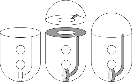
Figure 14. Left, the arc configuration $\mathcal{A}$ on $F$ with $g(F)=2$. Middle, gluing $(F\times[-1,1],\Xi_{\mathcal{A}})$ to $(D^{2}\times[-1,1],\xi_{D^{2}})$ with the negative region shaded. Right, $(D^{2}\cup F)$ with the annulus $A(c)$ shaded.

Proposition 3.27.

The invariant $\psi^{g}(B^{3},S^{1},\xi_{std})$ is a unit in $\textbf{{\text@underline{SHM}}}(-B^{3},-S^{1})\cong\mathcal{R}.$

Proof.

It follows from work of Niederkrüger and Wendl (see [38, Theorem 5]) that the contact manifold $((D^{2}\cup F)\times S^{1},\bar{\xi})$ is weakly symplectically fillable by some $(W,\omega)$. According to their construction, we may choose the curve $\eta$ so that $r(\eta\times\{0\})$ is, up to a scalar multiple, the Poincaré dual of $[\omega|_{(D^{2}\cup F)\times S^{1}}]$. Since $\underline{SHM}(-\mathscr{D})$ is defined with respect to the local system $\Gamma_{-\eta}$, it follows from Theorem 2.21 that the contact class $\psi(\mathscr{D},\bar{\xi})$ is a primitive element of $\underline{SHM}(-\mathscr{D})$. The proposition then follows from the fact that $\underline{SHM}(-\mathscr{D})\cong\mathcal{R}$, by Proposition 2.18. ∎

Remark 3.28.

The proof of Proposition 3.27 highlights the need for working with twisted coefficients: the contact structure $\bar{\xi}$ above is only weakly fillable and, indeed, Wendl shows in [51, Corollary 2] that its untwisted ECH contact invariant vanishes, from which it follows that $\psi(\mathscr{D},\bar{\xi})\in SHM(-\mathscr{D})$ vanishes as well.

Below, we compute the contact invariants of product manifolds built from general surfaces.

Let $S$ be a genus $k$ surface with $l\geq 1$ boundary components. Consider the $[-1,1]$-invariant contact structure $\xi_{S}$ on $S\times[-1,1]$ for which each $S\times\{t\}$ is convex with collared Legendrian boundary and the dividing set on $S\times\{1\}$ consists of $k$ boundary parallel arcs, one for each component of $\partial S$, oriented in the same direction as the boundary. See Figure 15. Let $H(S)$ be the product sutured contact handlebody of genus $2k+l-1$ obtained from $(S\times[-1,1],\partial S\times\{0\},\xi_{S})$ by rounding corners. Note that $H(S)$ is precisely the sort of contact handlebody that appears in the Heegaard splitting associated to an open book with page $S$.

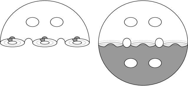
Figure 15. Left, $(S\times[-1,1],\xi_{S})$, with negative region shaded, for $k=2,l=3$. Right, the convex boundary of the product sutured contact handlebody $H(S)$ obtained by rounding corners.

We have the following generalization of Proposition 3.27.

Proposition 3.29.

The invariant $\psi^{g}(H(S))$ is a unit in $\textbf{{\text@underline{SHM}}}(-H(S))\cong\mathcal{R}$.

Proof.

This proof is virtually identical to that of Proposition 3.27. We start by constructing a genus $g$ marked contact closure of $H(S)$ for every

(19) $$g\geq g(H(S))=\max\{2,k+l\}=\max\{2,g(S)+|\partial S|\}.$$

Let $F$ be a surface with $l$ boundary components, and let $\mathcal{A}=\{c,a_{1},\dots,a_{l}\}$ be an arc configuration on $F$ with one arc meeting each boundary component. We form a genus $k+l+g(F)-1$ contact preclosure of $H(S)$ by gluing $(F\times[-1,1],\Xi_{\mathcal{A}})$ to $(S\times[-1,1],\xi_{S})$ and then proceed as in the case of the Darboux ball to construct a marked contact closure of the form $(\mathscr{D},\bar{\xi})$ with

$$\mathscr{D}=((S\cup F)\times S^{1},(S\cup F),r,m,\eta),$$

where $\bar{\xi}$ is an $S^{1}$-invariant contact structure for which the negative region on each fiber is a nonseparating annulus. These are exactly the same $S^{1}$-invariant contact manifolds as were considered in the proof of Proposition 3.27. Thus, for an appropriate choice of $\eta$, the contact class $\psi(\mathscr{D},\bar{\xi})$ is a unit in $\underline{SHM}(-\mathscr{D})\cong\mathcal{R}$. ∎

4. The well-definedness of $\psi^{g}(M,\Gamma,\xi)$ and $\psi(M,\Gamma,\xi)$

We prove Theorems 3.14 and 3.15 in the next two subsections. On the way to our proof of Theorem 3.15, we define maps on SHM associated to contact handle attachments and prove Propositions 3.26 and 3.23.

4.1. The well-definedness of $\psi^{g}(M,\Gamma,\xi)$

We start by describing the isomorphism $\underline{\Psi}_{-\mathscr{D}_{1},-\mathscr{D}_{2}}$ for $g(\mathscr{D}_{1})=g(\mathscr{D}_{2})$, as given in [3] but tailored slightly to our setting. We then prove Theorem 3.14, which implies that $\psi^{g}(M,\Gamma,\xi)\in\textbf{{\text@underline{SHM}}}(-M,-\Gamma)$ is well-defined.

Suppose

$$(\mathscr{D}_{1},\bar{\xi}_{1}) =((Y_{1},R_{1},r_{1},m_{1},\eta_{1}),\bar{\xi}_{1})$$

$$(\mathscr{D}_{2},\bar{\xi}_{2}) =((Y_{2},R_{2},r_{2},m_{2},\eta_{2}),\bar{\xi}_{2})$$

are two marked contact closures of $(M,\Gamma,\xi)$ of genus $g\geq g(M,\Gamma)$. To define $\underline{\Psi}_{-\mathscr{D}_{1},-\mathscr{D}_{2}}$, we first choose a contactomorphism

$$C:(Y_{1}\smallsetminus{\rm int}({\rm Im}(r_{1})),\bar{\xi}_{1})\to(Y_{2}\smallsetminus{\rm int}({\rm Im}(r_{2})),\bar{\xi}_{2})$$

which restricts to $m_{2}\circ m_{1}^{-1}$ on $m_{1}(M\smallsetminus N(\Gamma))$ for some neighborhood $N(\Gamma)$ of $\Gamma$. A contactomorphism of this form exists by Theorem 3.3. (Technically, Theorem 3.3 says that there is a contactomorphism of this form after applying flexibility to one of the complements above. However, we will ignore this point, as we can achieve the same effect by modifying one of the $\bar{\xi}_{i}$ via an arbitrarily small isotopy supported away from $m_{i}(M)$.) Let $\varphi_{\pm}$ and $\varphi$ be the diffeomorphisms defined by

$$\varphi_{\pm} =(r_{2}^{\pm})^{-1}\circ C\circ r_{1}^{\pm}:R_{1}\to R_{2}$$

$$\varphi =(\varphi_{+})^{-1}\circ\varphi_{-}:R_{1}\to R_{1},$$

where $r_{i}^{\pm}$ is the composition

$$R_{i}\xrightarrow{id\times\{\pm 1\}}R_{i}\times\{\pm 1\}\xrightarrow{r_{i}}Y_{i}.$$

Remark 3.2 implies that the negative region of $\bar{\xi}_{i}$ on each $r_{i}(R_{i}\times\{t\})$ is of the form $r_{i}(A_{i}\times\{t\})$ for some annulus $A_{i}\subset R_{i}$. Since $C$ is a contactomorphism, $\varphi_{\pm}$ sends $A_{1}$ to $A_{2}$, which implies that $\varphi$ sends $A_{1}$ to itself. Let

$$\psi:R_{1}\to R_{1}$$

be any diffeomorphism such that $\psi$ sends $A_{1}$ to itself and

$$(\varphi_{-}\circ\psi)(\eta_{1})=\eta_{2}.$$

Remark 4.1.

The diffeomorphisms above are defined so that the triple $(Y_{2},r_{2}(R_{2}\times\{0\}),\eta_{2})$ is diffeomorphic to that obtained from $(Y_{1},r_{1}(R_{1}\times\{0\}),\eta_{1})$ by cutting the latter open along the surfaces $r_{1}(R_{1}\times\{t\})$ and $r_{1}(R_{1}\times\{t^{\prime}\})$ for some $t<0<t^{\prime}$ and regluing by the maps $r_{1}\circ\psi^{-1}\circ r_{1}^{-1}$ and $r_{1}\circ(\varphi\circ\psi)\circ r_{1}^{-1}.$ By expressing these maps as compositions of Dehn twists, we can realize this cutting and regluing operation via surgery. The isomorphism $\underline{\Psi}_{-\mathscr{D}_{1},-\mathscr{D}_{2}}$ is then defined in terms of 2-handle cobordism maps associated to such surgeries, as below.

Since $\varphi\circ\psi$ and $\psi^{-1}$ fix the annulus $A_{1}$, these diffeomorphisms are isotopic to compositions of Dehn twists about nonseparating curves $a_{1},\dots,a_{m}\subset R_{1}\smallsetminus\partial A_{1}$,

$$\varphi\circ\psi \sim D^{e_{1}}_{a_{1}}\circ\cdots\circ D^{e_{n}}_{a_{n}}$$

$$\psi^{-1} \sim D^{e_{n+1}}_{a_{n+1}}\circ\cdots\circ D^{e_{m}}_{a_{m}}.$$

Here $D_{a_{i}}$ is a positive Dehn twist about $a_{i}$, and $e_{i}\in\{\pm 1\}$.

We next choose real numbers

$$-3/4<t_{m}<\dots<t_{n+1}<-1/4<1/4<t_{n}<\dots<t_{1}<3/4,$$

and pick some $t_{i}^{\prime}$ between $t_{i}$ and the next greatest number in this list for every $i$ such that $e_{i}=+1.$ Let $(Y_{1})_{-}$ be the 3-manifold obtained from $Y_{1}$ by performing $(-1)$-surgeries on the curves $r_{1}(a_{i}\times\{t_{i}\})$ for which $e_{i}=+1$, with respect to the framings induced by the surfaces $r_{1}(R_{1}\times\{t_{i}\})$. Let $X_{-}$ be the 4-manifold obtained by attaching $(+1)$-framed 2-handles to $(Y_{1})_{-}\times[0,1]$ along the curves $r_{1}(a_{i}\times\{t_{i}^{\prime}\})\times\{1\}$ for which $e_{i}=+1$. One boundary component of $X_{-}$ is $-(Y_{1})_{-}$. The other is canonically (up to isotopy) diffeomorphic to $Y_{1}$ since the $(+1)$-surgery on $r_{1}(a_{i}\times\{t_{i}^{\prime}\})$ cancels the $(-1)$-surgery on $r_{1}(a_{i}\times\{t_{i}\})$. We may therefore view $X_{-}$ as a cobordism from $(Y_{1})_{-}$ to $Y_{1}$. This cobordism gives rise to a map

$$\widecheck{\mathit{HM}}_{\bullet}({-}X_{-}|{-}R_{1};\Gamma_{-\nu}):\widecheck{\mathit{HM}}_{\bullet}(-(Y_{1})_{-}|{-}R_{1};\Gamma_{-\eta_{1}})\to\widecheck{\mathit{HM}}_{\bullet}(-Y_{1}|{-}R_{1};\Gamma_{-\eta_{1}}),$$

where $\nu$ is the cylinder $\nu=r_{1}(\eta_{1}\times\{0\})\times[0,1]\subset X_{-}$.

Similarly, let $X_{+}$ be the 4-manifold obtained from $(Y_{1})_{-}\times[0,1]$ by attaching $(+1)$-framed 2-handles along the curves $r_{1}(a_{i}\times\{t_{i}\})\times\{1\}$ for which $e_{i}=-1$. The boundary of $X_{+}$ is the union of $-(Y_{1})_{-}$ with the 3-manifold $(Y_{1})_{+}$ obtained from $(Y_{1})_{-}$ by performing $(+1)$-surgeries on the curves $r_{1}(a_{i}\times\{t_{i}\})$ for which $e_{i}=-1$. Thus, $X_{+}$ gives rise to a map

$$\widecheck{\mathit{HM}}_{\bullet}({-}X_{+}|{-}R_{1};\Gamma_{-\nu}):\widecheck{\mathit{HM}}_{\bullet}(-(Y_{1})_{-}|{-}R_{1};\Gamma_{-\eta_{1}})\to\widecheck{\mathit{HM}}_{\bullet}(-(Y_{1})_{+}|{-}R_{1};\Gamma_{-\eta_{1}}),$$

where $\nu=r_{1}(\eta_{1}\times\{0\})\times[0,1]\subset X_{+}$ in this case. This map and the one above are shown to be isomorphisms in [3].

As suggested in Remark 4.1, there is a unique isotopy class of diffeomorphisms

$$\bar{C}:(Y_{1})_{+}\to Y_{2}$$

which restricts to $C$ on $Y_{1}\smallsetminus{\rm int}({\rm Im}(r_{1}))\subset(Y_{1})_{+}$. Let

$$\Theta^{\bar{C}}:\widecheck{\mathit{HM}}_{\bullet}({-}(Y_{1})_{+}|{-}R_{1};\Gamma_{-\eta_{1}})\to\widecheck{\mathit{HM}}_{\bullet}({-}Y_{2}|{-}R_{2};\Gamma_{-\eta_{2}})$$

be the isomorphism on monopole Floer homology induced by $\bar{C}$. The map

$$\underline{\Psi}_{-\mathscr{D}_{1},-\mathscr{D}_{2}}:\widecheck{\mathit{HM}}_{\bullet}({-}Y_{1}|{-}R_{1};\Gamma_{-\eta_{1}})\to\widecheck{\mathit{HM}}_{\bullet}({-}Y_{2}|{-}R_{2};\Gamma_{-\eta_{2}})$$

is defined to be the composition

$$\underline{\Psi}_{-\mathscr{D}_{1},-\mathscr{D}_{2}}=\Theta^{\bar{C}}\circ\widecheck{\mathit{HM}}_{\bullet}({-}X_{+}|{-}R_{1};\Gamma_{-\nu})\circ\widecheck{\mathit{HM}}_{\bullet}({-}X_{-}|{-}R_{1};\Gamma_{-\nu})^{-1}.$$

In [3], we proved that this map is independent of the choices made in its construction, up to multiplication by a unit in $\mathcal{R}$. Having defined $\underline{\Psi}_{-\mathscr{D}_{1},-\mathscr{D}_{2}}$, we may now prove Theorem 3.14.

Proof of Theorem 3.14.

It suffices to show that

$$\underline{\Psi}_{-\mathscr{D}_{1},-\mathscr{D}_{2}}(\psi(\mathscr{D}_{1},\bar{\xi}_{1}))\doteq\psi(\mathscr{D}_{2},\bar{\xi}_{2})$$

for the marked contact closures $(\mathscr{D}_{1},\bar{\xi}_{1})$ and $(\mathscr{D}_{2},\bar{\xi}_{2})$ above. Note that the curves $r_{1}(a_{i}\times\{t_{i}\})$ and $r_{1}(a_{i}\times\{t_{i}^{\prime}\})$ are nonisolating in $r_{1}(R_{1}\times\{t_{i}\})$ and $r_{1}(R_{1}\times\{t_{i}^{\prime}\})$ since each component of $R_{1}\smallsetminus a_{i}$ intersects $\partial A_{1}$. We can therefore make these curves Legendrian for all $i=1,\dots,m$ by isotoping $\bar{\xi}_{1}$ slightly, according to the Legendrian Realization Principle [23, 17]. In a slight abuse of notation, let us simply assume that these curves are Legendrian with respect to $\bar{\xi}_{1}$. The surface framings on these Legendrian curves agree with their contact framings since the curves are disjoint from the dividing sets on their respective surfaces (each $a_{i}$ is disjoint from $\partial A_{1}$). In particular, we can arrange that the $(\pm 1)$-surgeries performed in defining $\underline{\Psi}_{-\mathscr{D}_{1},-\mathscr{D}_{2}}$ are actually contact $(\pm 1)$-surgeries. Let $(\bar{\xi}_{1})_{\pm}$ be the contact structures on $(Y_{1})_{\pm}$ induced by these surgeries. Since $(+1)$-surgery on $r_{1}(a_{i}\times\{t_{i}^{\prime}\})$ cancels $(-1)$-surgery on $r_{1}(a_{i}\times\{t_{i}\})$ contact geometrically as well as topologically, we have that

$$\widecheck{\mathit{HM}}_{\bullet}({-}X_{-}|{-}R_{1};\Gamma_{-\nu})(\psi((Y_{1})_{-},(\bar{\xi}_{1})_{-}))\doteq\psi(\mathscr{D}_{1},\bar{\xi}_{1})$$

by Corollary 2.23. The same corollary tells us that

$$\widecheck{\mathit{HM}}_{\bullet}({-}X_{+}|{-}R_{1};\Gamma_{-\nu})(\psi((Y_{1})_{-},(\bar{\xi}_{1})_{-}))\doteq\psi((Y_{1})_{+},(\bar{\xi}_{1})_{+}).$$

Finally, we can arrange that the diffeomorphism $\bar{C}$ is a contactomorphism, which implies

$$\Theta^{\bar{C}}(\psi((Y_{1})_{+},(\bar{\xi}_{1})_{+}))\doteq\psi(\mathscr{D}_{2},\bar{\xi}_{2}).$$

Putting these pieces together, we have that

$$\underline{\Psi}_{-\mathscr{D}_{1},-\mathscr{D}_{2}}(\psi(\mathscr{D}_{1},\bar{\xi}_{1}))\doteq\psi(\mathscr{D}_{2},\bar{\xi}_{2}).$$

completing the proof. ∎

4.2. The well-definedness of $\psi(M,\Gamma,\xi)$

We start by describing the isomorphism $\underline{\Psi}_{-\mathscr{D}_{1},-\mathscr{D}_{2}}$ in the case that $g(\mathscr{D}_{1})\neq g(\mathscr{D}_{2})$. The exposition here is tailored to the setting of contact closures and therefore differs slightly from that in [3]. We then define contact handle attachment maps and prove Theorem 3.15, which implies that $\psi(M,\Gamma,\xi)\in\textbf{{\text@underline{SHM}}}(-M,-\Gamma)$ is well-defined.

Suppose $(\mathscr{D}_{1},\bar{\xi}_{1})$ and $(\mathscr{D}_{2},\bar{\xi}_{2})$ are marked contact closures of $(M,\Gamma,\xi)$. Let us first consider the case in which

$$g(\mathscr{D}_{2})=g(\mathscr{D}_{1})+1=g+1.$$

To define $\underline{\Psi}_{-\mathscr{D}_{1},-\mathscr{D}_{2}}$, we first construct two additional marked contact closures as follows. Let $F$ be an auxiliary surface such that the closed surface formed by gluing $F$ to $R_{+}(\Gamma)$ has genus $g+1$. Then $F$ has genus at least two since $\mathscr{D}_{1}$ is formed from an auxiliary surface of genus at least one and $g(\mathscr{D}_{1})=g$. It follows that there is an embedded subsurface $\Sigma\subset{\rm int}(F)$ of genus one with two boundary components $c_{1},c_{2}\subset{\rm int}(F)$ such that $F\smallsetminus\Sigma$ is connected. Let $\mathcal{A}=\{c,a_{1},\dots,a_{m}\}$ be an arc configuration on $F$ contained in $F\smallsetminus\Sigma$. Let $(M^{\prime},\xi^{\prime})$ be the contact preclosure formed from $F$, $\mathcal{A}$, and some choices of $A(\Gamma)$ and

$$h:\partial F\times[-1,1]\to A(\Gamma).$$

Note that the boundary components $\partial_{\pm}M^{\prime}$ have genus $g+1$. As usual, the negative region on $\partial_{+}M^{\prime}$ is an annular neighborhood $A(c)$ of $c$, by Remark 3.2. Let $R$ be a copy of $\partial_{+}M^{\prime}$ and let $(Y,\bar{\xi})$ be the closed contact manifold obtained by gluing $R\times[-1,1]$, equipped with the $[-1,1]$-invariant contact structure with negative region $A(c)\times\{t\}$ on each $R\times\{t\}$, to $M^{\prime}$ by diffeomorphisms

(20) $$R\times\{\pm 1\}\to\partial M^{\prime}_{\mp}$$

which restrict to the “identity” maps from $\Sigma\times\{\pm 1\}\subset R\times\{\pm 1\}$ to $\Sigma\times\{\mp 1\}\subset\partial M^{\prime}_{\mp}$. Let $\eta$ be a curve in $R$ dual to the core of $A(c)$ which restricts to a properly embedded arc on $\Sigma$. Then

$$(\mathscr{D}=(Y,R,r,m,\eta),\bar{\xi})$$

is a genus $g+1$ marked contact closure of $(M,\Gamma,\xi)$, where $r$ and $m$ are the obvious embeddings of $R\times[-1,1]$ and $M$ into $Y$.

Let $F^{\prime}$ be the surface obtained from $\overline{F\smallsetminus\Sigma}$ by gluing $c_{1}$ to $c_{2}$ via an orientation-reversing diffeomorphism

$$f:c_{1}\to c_{2}$$

which sends $c_{1}\cap\eta$ to $c_{2}\cap\eta$, as shown in Figure 16. Since $\mathcal{A}$ is disjoint from $\Sigma$, it descends to an arc configuration on $F^{\prime}$. Let $(M^{\prime\prime},\xi^{\prime\prime})$ be the contact preclosure formed from $F^{\prime}$, $\mathcal{A}$, $A(\Gamma)$, and $h$. Note that the boundary components $\partial M^{\prime\prime}_{\pm}$ are obtained from $\partial M^{\prime}_{\pm}$ by removing $\Sigma\times\{\pm 1\}$ and gluing $c_{1}\times\{\pm 1\}$ to $c_{2}\times\{\pm 1\}$ by $f$. Let $R^{\prime}$ be a copy of $\partial M^{\prime\prime}_{\pm}$ and let $(Y^{\prime},\bar{\xi}^{\prime})$ be the closed contact manifold obtained by gluing $R^{\prime}\times[-1,1]$, equipped with the $[-1,1]$-invariant contact structure with negative region $A(c)\times\{t\}$ on each $R\times\{t\}$, to $M^{\prime\prime}$ by the diffeomorphisms

$$R^{\prime}\times\{\pm 1\}\to\partial M^{\prime\prime}_{\mp}$$

induced by those in (20). Then

$$(\mathscr{D}^{\prime}=(Y^{\prime},R^{\prime},r^{\prime},m^{\prime},\eta^{\prime}),\bar{\xi}^{\prime})$$

is a genus $g$ marked contact closure of $(M,\Gamma,\xi)$, where $r^{\prime}$ and $m^{\prime}$ are the embeddings naturally induced by $r$ and $m$ and $\eta^{\prime}\subset R^{\prime}$ is the curve induced by $\eta$.

$\eta$ at 91 97 $\eta^{\prime}$ at 247 97 $c_{1}$ at 17 62 $c_{2}$ at 106 62 $c$ at 62 54 $c$ at 215 54

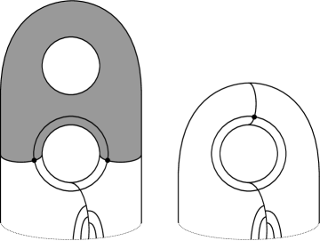
Figure 16. Left, a portion of the surface $F$ with the region $\Sigma$ shaded. Right, the surface $F^{\prime}$. The arc configuration $\mathcal{A}$ is shown in red, intersecting $\eta$ and $\eta^{\prime}$ along the curve $c$.

The isomorphism $\underline{\Psi}_{-\mathscr{D}^{\prime},-\mathscr{D}}$ is defined in terms of a splicing cobordism $W$, described below. Once we have defined this isomorphism, we define $\underline{\Psi}_{-\mathscr{D}_{1},-\mathscr{D}_{2}}$ as in (21). In defining $W$, the important observation is that the union of annuli

$$(c_{i}\times[-1,1]\subset F\times[-1,1]\subset M^{\prime})\,\,\cup\,\,(c_{i}\times[-1,1]\subset R\times[-1,1])$$

is an embedded torus $T_{i}=c_{i}\times S^{1}\subset Y$ for $i=1,2$. Together, these tori cut $Y$ into pieces $Y_{M}$ and $Y_{\Sigma}$ with

$$-\partial Y_{M}=\partial Y_{\Sigma}=T_{1}\cup T_{2}.$$

In particular, $Y_{M}$ is the piece that contains $M$ and $Y_{\Sigma}$ is the mapping torus of some diffeomorphism of $\Sigma$. Note that the closed manifold obtained from $Y_{M}$ by gluing $T_{1}$ to $T_{2}$ by $f\times id$ is precisely $Y^{\prime}$, while the manifold obtained from $Y_{\Sigma}$ in this way is a mapping torus $M(\Sigma^{\prime})$ of some diffeomorphism of $\Sigma^{\prime}$, where $\Sigma^{\prime}$ is the closed genus two surface obtained from $\Sigma$ by gluing $c_{1}$ to $c_{2}$ by $f$. Let $\eta_{\Sigma^{\prime}}\subset\Sigma^{\prime}$ be the curve induced by $\eta$. The splicing cobordism

$$W:Y^{\prime}\sqcup M(\Sigma^{\prime})\to Y$$

is then defined by gluing the products $Y_{M}\times[0,1]$ and $Y_{\Sigma}\times[0,1]$ to $T_{1}\times S$, where $S$ is the saddle cobordism depicted in Figure 17. We glue these pieces along the “horizontal” portions of their boundaries according to the schematic in that figure, making use of the map $f\times id$. This cobordism induces a map

$$\widecheck{\mathit{HM}}_{\bullet}({-}W|{-}R^{\prime};\Gamma_{{-}\nu}) :\widecheck{\mathit{HM}}_{\bullet}({-}Y^{\prime}|{-}R^{\prime};\Gamma_{{-}\eta^{\prime}})\otimes_{\mathcal{R}}\widecheck{\mathit{HM}}_{\bullet}(-M(\Sigma^{\prime})|{-}\Sigma^{\prime};\Gamma_{{-}\eta_{\Sigma^{\prime}}})$$

$$\to\widecheck{\mathit{HM}}_{\bullet}({-}Y|{-}R;\Gamma_{{-}\eta}),$$

where $\nu\subset W$ is a pair-of-pants cobordism from $\eta^{\prime}\sqcup\eta_{\Sigma^{\prime}}$ to $\eta$. We define

$$\underline{\Psi}_{-\mathscr{D}^{\prime},-\mathscr{D}}(-)=\widecheck{\mathit{HM}}_{\bullet}({-}W|{-}R^{\prime};\Gamma_{{-}\nu})(-\otimes 1),$$

where $1$ is a generator of $\widecheck{\mathit{HM}}_{\bullet}(-M(\Sigma^{\prime})|{-}\Sigma^{\prime};\Gamma_{{-}\eta_{\Sigma^{\prime}}})\cong\mathcal{R}$. We then define

(21) $$\underline{\Psi}_{-\mathscr{D}_{1},-\mathscr{D}_{2}}=\underline{\Psi}_{-\mathscr{D},-\mathscr{D}_{2}}\circ\underline{\Psi}_{-\mathscr{D}^{\prime},-\mathscr{D}}\circ\underline{\Psi}_{-\mathscr{D}_{1},-\mathscr{D}^{\prime}}.$$

Here, $\underline{\Psi}_{-\mathscr{D},-\mathscr{D}_{2}}$ and $\underline{\Psi}_{-\mathscr{D}_{1},-\mathscr{D}^{\prime}}$ are the maps defined in the previous subsection for closures of the same genus.

$S$ at 142 130 $T_{1}\times S$ at 490 130 $Y_{M}\times[0,1]$ at 490 239 $Y_{\Sigma}\times[0,1]$ at 490 18 $Y^{\prime}$ at 346 207 $Y$ at 620 130 $M(\Sigma^{\prime})$ at 332 53

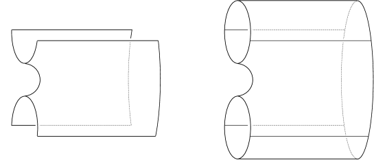
Figure 17. Left, the saddle $S$. Right, a schematic of the splicing cobordism $W$.

In the case that $g(\mathscr{D}_{2})=g(\mathscr{D}_{1})-1$, we define

$$\underline{\Psi}_{-\mathscr{D}_{1},-\mathscr{D}_{2}}=\underline{\Psi}_{-\mathscr{D}_{2},-\mathscr{D}_{1}}^{-1}.$$

For the general case, we choose a sequence $(\mathscr{D}^{1},\bar{\xi}^{1}),\dots,(\mathscr{D}^{n},\bar{\xi}^{n})$ of marked contact closures of $(M,\Gamma,\xi)$ such that $(\mathscr{D}^{1},\bar{\xi}^{1})=(\mathscr{D}_{1},\bar{\xi}_{1})$, $(\mathscr{D}^{n},\bar{\xi}^{n})=(\mathscr{D}_{2},\bar{\xi}_{2})$, and

$$|g(\mathscr{D}^{i+1})-g(\mathscr{D}^{i})|\leq 1$$

for all $i=1,\dots,n-1$. Then we define

$$\underline{\Psi}_{-\mathscr{D}_{1},-\mathscr{D}_{2}}=\underline{\Psi}_{-\mathscr{D}^{n-1},-\mathscr{D}^{n}}\circ\dots\circ\underline{\Psi}_{-\mathscr{D}^{1},-\mathscr{D}^{2}}.$$

We proved in [3] that this map is independent of the choices made in its construction, up to multiplication by a unit in $\mathcal{R}$.

Below, we define maps on SHM associated to contact $0$-, $1$-, $2$-, and $3$-handle attachments. We will use the $2$-handle attachment maps at the end to prove Theorem 3.15, which implies that the elements $\psi^{g}(M,\Gamma,\xi)$ are equal for large $g$ and, hence, that $\psi(M,\Gamma,\xi)$ is well-defined.

4.2.1. $0$-handle attachments

Attaching a contact $0$-handle to $(M,\Gamma,\xi)$ is equivalent to taking the disjoint union of $(M,\Gamma,\xi)$ with the Darboux ball $(B^{3},S^{1},\xi_{std})$. Let $(M_{0},\Gamma_{0},\xi_{0})$ be this disjoint union. We claim that every marked contact closure of $(M_{0},\Gamma_{0},\xi_{0})$ is a marked contact closure of $(M,\Gamma,\xi)$. To see this, think of the Darboux ball as the product sutured contact manifold $(D^{2}\times[-1,1],\partial D^{2}\times\{0\},\xi_{D^{2}})$, as in Subsection 3.4. Let $F_{0}$ be an auxiliary surface for $(M_{0},\Gamma_{0},\xi_{0})$ with arc configuration $\mathcal{A}_{0}=\{c,a_{1},\dots,a_{m}\}$ so that $a_{1}$ is the unique arc meeting the boundary component $\partial_{1}F_{0}$. We form a contact preclosure $(M^{\prime}_{0},\xi^{\prime}_{0})$ of $(M_{0},\Gamma_{0},\xi_{0})$ by attaching $F_{0}\times[-1,1]$ to $M_{0}$ such that $\partial_{1}F_{0}\times[-1,1]$ is glued to $\partial D^{2}\times[-1,1]$ by a map

$$h:\partial_{1}F_{0}\times[-1,1]\to\partial D^{2}\times[-1,1]$$

of the form $f\times{\rm id}$ for some diffeomorphism $f:\partial_{1}F_{0}\to\partial D^{2}$. Let $A(c)$ denote the negative annular region on $\partial_{+}M^{\prime}_{0}$. Let $R$ be a copy of $\partial_{+}M^{\prime}_{0}$. Let $(Y_{0},\bar{\xi}_{0})$ be the closed contact manifold obtained by gluing $R\times[-1,1]$, equipped with the $[-1,1]$-invariant contact structure with negative region $A(c)\times\{t\}$ on each $R\times\{t\}$, to $M^{\prime}_{0}$ by diffeomorphisms

$$R\times\{\pm 1\}\to\partial_{\mp}M^{\prime}_{0}$$

which identify dividing sets. Let $\eta$ be a curve in $R$ dual to the core of $A(c)$. Then

$$(\mathscr{D}_{0}=(Y_{0},R,r,m_{0},\eta),\bar{\xi}_{0})$$

is a marked contact closure of $(M_{0},\Gamma_{0},\xi_{0})$, where $r$ and $m_{0}$ are the obvious embeddings of $R\times[-1,1]$ and $M_{0}$ into $Y$.

Note that $(M^{\prime}_{0},\xi^{\prime}_{0})$ is a contact preclosure of $(M,\Gamma,\xi)$ as well, formed from the auxiliary surface $F=F_{0}\cup_{f}D^{2}$ and the arc configuration $\mathcal{A}=\{c,a_{2},\dots,a_{m}\}$. Thus,

$$(\mathscr{D}=(Y_{0},R,r,m,\eta),\bar{\xi}=\bar{\xi}_{0})$$

is a marked contact closure of $(M,\Gamma,\xi)$, where $m$ is the restriction of $m_{0}$ to $M$. In particular, $\underline{SHM}(-\mathscr{D})=\underline{SHM}(-\mathscr{D}_{0})$. We define the $0$-handle attachment map

$$\mathscr{H}_{0}:\textbf{{\text@underline{SHM}}}(-M,-\Gamma)\to\textbf{{\text@underline{SHM}}}(-M_{0},-\Gamma_{0})$$

to be the morphism determined by the equivalence class of the identity map from $\underline{SHM}(-\mathscr{D})$ to $\underline{SHM}(-\mathscr{D}_{0})$, which we will denote in this case by

$$id_{-\mathscr{D},-\mathscr{D}_{0}}:\underline{SHM}(-\mathscr{D})\to\underline{SHM}(-\mathscr{D}_{0}).$$

To prove that $\mathscr{H}_{0}$ is well-defined, we need only show that if $(\mathscr{D}_{0},\bar{\xi}_{0})$ and $(\mathscr{D}_{0}^{\prime},\bar{\xi}^{\prime}_{0})$ are marked contact closures of $(M_{0},\Gamma_{0},\xi_{0})$ constructed as above, and $(\mathscr{D},\bar{\xi})$ and $(\mathscr{D}^{\prime},\bar{\xi}^{\prime})$ are the corresponding marked contact closures of $(M,\Gamma,\xi)$, then the diagram

commutes, up to multiplication by a unit in $\mathcal{R}$. But this is clear: $\underline{\Psi}_{-\mathscr{D}_{0},-\mathscr{D}_{0}^{\prime}}$ is a composition of maps associated to 2-handle and splicing cobordisms, and $\underline{\Psi}_{-\mathscr{D},-\mathscr{D}^{\prime}}$ can be defined via the exact same composition. Note that

$$id_{-\mathscr{D},-\mathscr{D}_{0}}(\psi(\mathscr{D},\bar{\xi}))\doteq\psi(\mathscr{D}_{0},\bar{\xi}_{0})$$

since $\psi(\mathscr{D},\bar{\xi})=\psi(\mathscr{D}_{0},\bar{\xi}_{0})$ in $\underline{SHM}(-\mathscr{D})=\underline{SHM}(-\mathscr{D}_{0})$. We therefore have the following.

Proposition 4.2.

$\mathscr{H}_{0}(\psi^{g}(M,\Gamma,\xi))=\psi^{g}(M_{0},\Gamma_{0},\xi_{0})$ for each $g\geq g(M,\Gamma)$. ∎

4.2.2. $1$-handle attachments

Suppose $D_{-}$ and $D_{+}$ are disjoint embedded disks in $\partial M$ which each intersect $\Gamma$ in a single properly embedded arc. To attach a contact $1$-handle to $(M,\Gamma,\xi)$ along these disks, we glue $(D^{2}\times[-1,1],\xi_{D^{2}})$ to $(M,\Gamma,\xi)$ by diffeomorphisms

$$D^{2}\times\{-1\}\to D_{-}\ \ {\rm and}\ \ D^{2}\times\{+1\}\to D_{+},$$

which preserve and reverse orientations, respectively, and identify dividing sets, and then we round corners, as illustrated in Figure 18. Let $(M_{1},\Gamma_{1},\xi_{1})$ be the resulting sutured contact manifold. As in the $0$-handle case, we claim that every marked contact closure of $(M_{1},\Gamma_{1},\xi_{1})$ is also a marked contact closure of $(M,\Gamma,\xi)$.

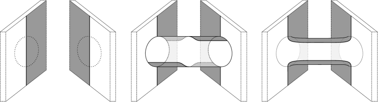
Figure 18. Left, a portion of a vertical invariant neighborhood of $\partial M$ near the disks $D_{-},D_{+}\subset\partial M$, whose boundaries are dotted. Middle, attaching the contact $1$-handle. Right, the $1$-handle attachment after rounding corners.

The rough idea is that if $F_{1}$ is an auxiliary surface for $(M_{1},\Gamma_{1})$, then, in the corresponding preclosure $M_{1}^{\prime}$, the union of $F_{1}\times[-1,1]$ with the contact $1$-handle is a product $F\times[-1,1]$, where $F$ is an auxiliary surface for $(M,\Gamma)$, so that $M_{1}^{\prime}$ is also a preclosure of $(M,\Gamma)$. We make this precise as follows. Choose an auxiliary surface $F_{1}$ for $(M_{1},\Gamma_{1})$, a neighborhood $A(\Gamma_{1})$, and a diffeomorphism

$$h_{1}:\partial F_{1}\times[-1,1]\to A(\Gamma_{1}).$$

We perturb $\xi_{1}$ as usual, so that, near the contact $1$-handle, the resulting dividing set intersects $A(\Gamma_{1})$ as shown in the upper right of Figure 19. We choose an arc configuration $\mathcal{A}_{1}$ on $F_{1}$ so that the negative region of $\Gamma_{\mathcal{A}_{1}}$ on a portion of the convex surface $F_{1}\times\{1\}\subset(F_{1}\times[-1,1],\Xi_{\mathcal{A}_{1}})$ glued near the $1$-handle consists of neighborhoods of four arcs, as shown in the lower right of Figure 19. Let $(M_{1}^{\prime},\xi_{1}^{\prime})$ denote the resulting contact preclosure of $(M_{1},\Gamma_{1},\xi_{1})$.

Let $\gamma_{+}$ and $\gamma_{-}$ be the arcs of $\partial F_{1}$ such that $\gamma_{\pm}\times\{1\}\subset\partial F_{1}\times\{1\}$ are mapped to the contact $1$-handle by $h_{1}$. Let $F$ be the surface obtained by attaching a two-dimensional $1$-handle to $F_{1}$ with feet at $\gamma_{\pm}$. Note that $F$ is an auxiliary surface for $(M,\Gamma)$. We use it to construct a contact preclosure of $(M,\Gamma,\xi)$ as follows. Let $A(\Gamma)\subset\partial M$ be a neighborhood of $\Gamma$ which agrees with $A(\Gamma_{1})$ outside of the attaching disks $D_{\pm}$. We perturb $\xi$ so that the resulting dividing set agrees with that of the perturbed $\xi_{1}$ outside of $D_{\pm}$ and is disjoint from $A(\Gamma)$ inside these disks, as shown in the upper left of Figure 19. By choosing $h_{1}$ more carefully to begin with, we can assume that it extends to a map

$$h:\partial F\times[-1,1]\to A(\Gamma)$$

which agrees with $h_{1}$ away from $\gamma_{\pm}\times[-1,1]$. Let $\mathcal{A}$ be the arc configuration on $F$ induced by $\mathcal{A}_{1}$, and let $(M^{\prime},\xi^{\prime})$ be the corresponding contact preclosure of $(M,\Gamma,\xi)$.

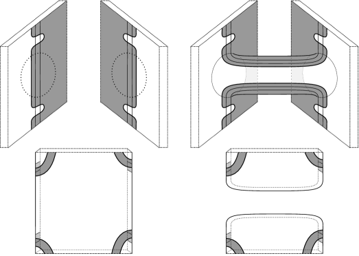
Figure 19. Upper left, a portion of a vertically invariant neighborhood of $\partial M$ near $D_{+},D_{-}$ showing $A(\Gamma)$ and the perturbed dividing set. Upper right, the corresponding portions of $M_{1}$ and $A(\Gamma_{1})$. Lower left, a portion of $F\times[-1,1]$ with the negative regions on $F\times\{1\}$ and $\partial F\times[-1,1]$ shaded. Lower right, the corresponding portion of $F_{1}\times[-1,1]$. The 3-balls $N\subset M^{\prime}$ and $N_{1}\subset M_{1}^{\prime}$ are obtained by gluing the portions of $F\times[-1,1]$ and $F_{1}\times[-1,1]$ shown here to the portions of $M$ and $M_{1}$ shown here via the maps $h$ and $h_{1}$.

Let $N\subset M^{\prime}$ be the 3-ball obtained by gluing the portion of $F\times[-1,1]$ shown in Figure 19 to the portion of $M$ shown there, and define $N_{1}\subset M_{1}^{\prime}$ analogously. Note that

(22) $$(M^{\prime}\smallsetminus N,\xi^{\prime})=(M_{1}^{\prime}\smallsetminus N_{1},\xi_{1}^{\prime}).$$

We claim that, after rounding corners, $N$ and $N_{1}$ are Darboux balls. This will imply that the identity map on the manifold in (22) extends (uniquely, up to isotopy) to a contactomorphism

$$(M^{\prime},\xi^{\prime})\to(M_{1}^{\prime},\xi_{1}^{\prime}).$$

For the claim, it is enough to show that $N$ and $N_{1}$ are tight (as there is a unique tight ball). But since $N$ and $N_{1}$ only depend on $\xi$ on a vertically invariant neighborhood of $\partial M$, it suffices to find some $(M,\Gamma,\xi)$ such that all contact preclosures of $(M,\Gamma,\xi)$ and $(M_{1},\Gamma_{1},\xi_{1})$ are tight. We can take $(M,\Gamma,\xi)$ to be the Darboux ball $(B^{3},S^{1},\xi_{std})$, in which case $(M_{1},\Gamma_{1},\xi_{1})$ is the product sutured contact handlebody $H(S)$ for a surface $S$ with genus $0$ and $2$ boundary components. It follows from the results in Subsections 3.4 and 4.1 that contact preclosures of both the Darboux ball and this handlebody are always tight, settling the claim.

Now, let $R$ be a copy of $\partial_{+}M^{\prime}_{1}$, and let $(Y_{1},\bar{\xi}_{1})$ be the closed contact manifold obtained by gluing $R\times[-1,1]$, equipped with the appropriate $[-1,1]$-invariant contact structure, to $M^{\prime}_{1}$ in the usual way. Consider the marked contact closure

$$(\mathscr{D}_{1}=(Y_{1},R,r,m_{1},\eta),\bar{\xi}_{1})$$

of $(M_{1},\Gamma_{1},\xi_{1})$, where $\eta$ is an appropriately chosen curve on $R$, and $r$ and $m_{1}$ are the obvious embeddings of $R\times[-1,1]$ and $M_{1}$ into $Y_{1}$. Since $(M^{\prime},\xi^{\prime})$ and $(M_{1}^{\prime},\xi_{1}^{\prime})$ are contactomorphic by the identity map outside of balls, we have that

$$(\mathscr{D}=(Y_{1},R,r,m,\eta),\bar{\xi}=\bar{\xi}_{1})$$

is a marked contact closure of $(M,\xi)$, where $m$ is the restriction of $m_{1}$ to $M$. In particular, $\underline{SHM}(-\mathscr{D})=\underline{SHM}(-\mathscr{D}_{1})$. We define the $1$-handle attachment map

$$\mathscr{H}_{1}:\textbf{{\text@underline{SHM}}}(-M,-\Gamma)\to\textbf{{\text@underline{SHM}}}(-M_{1},-\Gamma_{1})$$

to be the morphism determined by the equivalence class of the identity map from $\underline{SHM}(-\mathscr{D})$ to $\underline{SHM}(-\mathscr{D}_{1})$. The proof that $\mathscr{H}_{1}$ is well-defined is then exactly as in the $0$-handle case. Since the identity map $id_{-\mathscr{D},-\mathscr{D}_{1}}$ sends $\psi(\mathscr{D},\bar{\xi})$ to $\psi(\mathscr{D}_{1},\bar{\xi}_{1})$, we have the following.

Proposition 4.3.

$\mathscr{H}_{1}(\psi^{g}(M,\Gamma,\xi))=\psi^{g}(M_{1},\Gamma_{1},\xi_{1})$ for each $g\geq g(M,\Gamma)$. ∎

4.2.3. $2$-handle attachments

Suppose $\gamma$ is an embedded curve in $\partial M$ which intersects $\Gamma$ in two points. Let $A(\gamma)$ be an annular neighborhood of $\gamma$ intersecting $\Gamma$ in two cocores. To attach a contact $2$-handle to $(M,\Gamma,\xi)$ along $A(\gamma)$, we glue $(D^{2}\times[-1,1],\xi_{D^{2}})$ to $(M,\Gamma,\xi)$ by an orientation-reversing diffeomorphism

$$\partial D^{2}\times[-1,1]\to A(\gamma)$$

which identifies positive regions with negative regions, and then round corners, as illustrated in Figure 20. Let $(M_{2},\Gamma_{2},\xi_{2})$ be the resulting sutured contact manifold.

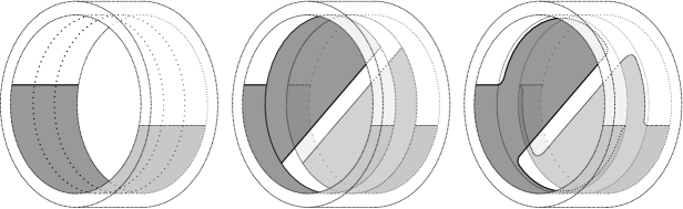
Figure 20. Left, a portion of a vertically invariant neighborhood of $\partial M$ near $A(\gamma)\subset\partial M$, whose boundary is dotted. This portion is a neighborhood $N$ of the Legendrian curve $\gamma^{\prime}$. Middle, attaching the contact $2$-handle. Right, the $2$-handle attachment after rounding corners.

Now, consider the sutured contact manifold $(M_{1},\Gamma_{1},\xi_{1})$ obtained from $(M_{2},\Gamma_{2},\xi_{2})$ by attaching a contact $1$-handle along disks in the interiors of the $D^{2}\times\{\pm 1\}$ boundary components of the contact $2$-handle, as indicated in Figure 21, and let

$$\mathscr{H}_{1}:\textbf{{\text@underline{SHM}}}(-M_{2},-\Gamma_{2})\to\textbf{{\text@underline{SHM}}}(-M_{1},-\Gamma_{1})$$

be the corresponding $1$-handle attachment map, as defined in Subsubsection 4.2.2. It is easy to see that $(M_{1},\Gamma_{1})$ is diffeomorphic to the sutured manifold obtained from $(M,\Gamma)$ by performing $\partial M$-framed surgery on a copy $\gamma^{\prime}$ of $\gamma$ in the interior of $M$. By the Legendrian Realization Principle, we can assume that $\gamma^{\prime}$ is Legendrian in $(M,\Gamma,\xi)$ since $\gamma$ is nonisolating in $\partial M$. Moreover, since $\gamma$ intersects $\Gamma$ in exactly two points, the $\partial M$-framing on $\gamma^{\prime}$ is one more than its contact framing. Below, we argue that $(M_{1},\Gamma_{1},\xi_{1})$ is in fact contactomorphic (by a canonical isotopy class of contactomorphisms) to the result of contact $(+1)$-surgery on $\gamma^{\prime}$.

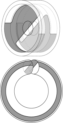
Figure 21. Attaching a contact $1$-handle to form $M_{1}$. The circles on $D^{2}\times\{\pm 1\}$ indicate where the feet of this handle are to be attached. The union of the $1$-handle below with the portion of $M_{1}$ shown above is the solid torus $N_{1}$.

To see this, let $N\subset M$ be the solid torus on the left in Figure 20 and let $N_{1}\subset M_{1}$ be the solid torus obtained from $N$ by attaching the $1$- and $2$-handles as indicated in Figures 20 and 21. After slight modification, $N$ and $N_{1}$ can be made to have convex boundaries. Note that

(23) $$(M\smallsetminus N,\Gamma,\xi)=(M_{1}\smallsetminus N_{1},\Gamma_{1},\xi_{1}).$$

Furthermore, the identity map, restricted to $\partial M\smallsetminus N=\partial M_{1}\smallsetminus N_{1}$, extends uniquely (up to isotopy) to a diffeomorphism

$$(\partial M,\Gamma)\to(\partial M_{1},\Gamma_{1}).$$

It follows that the identity map on the manifold in (23) extends uniquely (up to isotopy) to a contactomorphism

$$(M\smallsetminus N^{\prime},\Gamma,\xi)\to(M_{1}\smallsetminus N_{1}^{\prime},\Gamma_{1},\xi_{1}),$$

where $N^{\prime}\subset{\rm int}(N)$ is the solid torus with convex boundary obtained by removing a vertically invariant collar $\partial N\times[-\infty,0)$ from $N$, and $N^{\prime}_{1}$ is defined from $N_{1}$ analogously. In other words, there is a canonical contactomorphism (up to isotopy),

$$f:(M^{\prime},\Gamma^{\prime},\xi^{\prime})\to(M_{1},\Gamma_{1},\xi_{1}),$$

where $(M^{\prime},\Gamma^{\prime},\xi^{\prime})$ is the contact manifold obtained from $(M,\Gamma,\xi)$ by removing the solid torus neighborhood $N^{\prime}$ of $\gamma^{\prime}$ and gluing back in a solid torus contactomorphic to $N_{1}^{\prime}$ according to the contact framing on $\gamma^{\prime}$ plus one. To show that this operation is actually a contact $(+1)$-surgery, all that remains is to show that $N$ and $N_{1}$ are tight (as there is a unique tight solid torus with the given dividing set on its boundary).

Since $N$ and $N_{1}$ only depend on $\xi$ on a vertically invariant neighborhood of $\partial M$, it suffices to find some $(M,\Gamma,\xi)$ such that both $(M,\Gamma,\xi)$ and some sutured contact manifold obtained from $(M,\Gamma,\xi)$ by attaching contact $2$- and $1$-handles as above are tight. We can take $(M,\Gamma,\xi)$ to be the tight solid torus $H(S)$ for a surface $S$ with genus 0 and 2 boundary components. Etgü and Özbağcı show in [9, Example 3] that one can obtain the Darboux ball by attaching a contact $2$-handle to this solid torus. We proved in Proposition 3.27 that any marked contact closure $(\mathscr{D},\bar{\xi})$ of $(B^{3},S^{1},\xi_{std})$ has nonzero invariant $\psi(\mathscr{D},\bar{\xi})$. This then implies, by the earlier results in this section, that any marked contact closure of the sutured contact manifold obtained from the Darboux ball by attaching a contact $1$-handle also has nonzero invariant. The manifold resulting from this $1$-handle attachment is therefore tight as well.

Thus, $(M^{\prime},\Gamma^{\prime},\xi^{\prime})$ is obtained from $(M,\Gamma,\xi)$ via contact $(+1)$-surgery along the Legendrian curve $\gamma^{\prime}$.

In order to define the $2$-handle map $\mathscr{H}_{2}$, we first define the morphism $F_{K}$ in Proposition 3.26. Suppose

$$(\mathscr{D}=(Y,R,r,m,\eta),\bar{\xi})$$

is a marked contact closure of $(M,\Gamma,\xi)$. Let $(Y^{\prime},\bar{\xi}^{\prime})$ be the contact 3-manifold obtained from $Y$ by performing contact $(+1)$-surgery on $m(K)$ for some Legendrian knot $K\subset M$. Then

$$(\mathscr{D}^{\prime}=(Y^{\prime},R,r^{\prime},m^{\prime},\eta),\bar{\xi}^{\prime})$$

is a contact closure of $(M^{\prime},\Gamma^{\prime},\xi^{\prime})$, where $r^{\prime}$ is the map induced by $r$ and $m^{\prime}$ is the embedding of $M^{\prime}$ into $Y^{\prime}$ induced by $m$. Let $W$ be the $2$-handle cobordism from $Y$ to $Y^{\prime}$ corresponding to the above surgery. We define

$$F_{K}:\textbf{{\text@underline{SHM}}}(-M,-\Gamma)\to\textbf{{\text@underline{SHM}}}(-M^{\prime},-\Gamma^{\prime})$$

to be the morphism induced by the map

$$\widecheck{\mathit{HM}}_{\bullet}({-}W|{-}R;\Gamma_{-\nu}):\underline{SHM}(-\mathscr{D})\to\underline{SHM}(-\mathscr{D}^{\prime}),$$

where $\nu\subset W$ is the natural cylindrical cobordism from $r(\eta\times\{0\})\subset Y$ to $r^{\prime}(\eta\times\{0\})\subset Y^{\prime}$. To prove that $F_{K}$ is well-defined, we must show that the diagram

commutes, up to multiplication by a unit in $\mathcal{R}$, for any two marked contact closures $(\mathscr{D}_{1},\bar{\xi}_{1})$ and $(\mathscr{D}_{2},\bar{\xi}_{2})$ of $(M,\Gamma,\xi)$, where $(\mathscr{D}_{i}^{\prime},\bar{\xi}_{i}^{\prime})$ is the marked contact closure of $(M^{\prime},\Gamma^{\prime},\xi^{\prime})$ induced by $(\mathscr{D}_{i},\bar{\xi}_{i})$ and $W_{i}$ is the $2$-handle cobordism from $Y_{i}$ to $Y_{i}^{\prime}$. But this follows from the commutativity of the cobordisms used to define these maps: $W_{1}$ and $W_{2}$ are built by attaching $2$-handles along curves in the regions $m_{1}(M)$ and $m_{2}(M)$, while the vertical isomorphisms are defined from cobordisms built by attaching 2-handles or splicing along tori outside of these regions. Since $\widecheck{\mathit{HM}}_{\bullet}({-}W|{-}R;\Gamma_{-\nu})$ sends $\psi(\mathscr{D},\bar{\xi})$ to $\psi(\mathscr{D}^{\prime},\bar{\xi}^{\prime})$, by Corollary 2.23, we have the following, which proves Proposition 3.26.

Proposition 4.4.

$F_{K}(\psi^{g}(M,\Gamma,\xi))=\psi^{g}(M^{\prime},\Gamma^{\prime},\xi^{\prime})$ for each $g\geq g(M,\Gamma)$. ∎

We now define the $2$-handle attachment map

$$\mathscr{H}_{2}:\textbf{{\text@underline{SHM}}}(-M,-\Gamma)\to\textbf{{\text@underline{SHM}}}(-M_{2},-\Gamma_{2}),$$

to be the composition of morphisms

$$\mathscr{H}_{2}=\mathscr{H}_{1}^{-1}\circ\textbf{{\text@underline{SHM}}}(f)\circ F_{\gamma^{\prime}}.$$

That $\mathscr{H}_{2}$ is independent of $\gamma^{\prime}$ follows from the fact that any two such Legendrian realizations of $\gamma$ are related by an ambient isotopy of $M$ supported in $N$. Unpacking the composition above, we see that $\mathscr{H}_{2}$ may also be formulated as follows. Suppose $(\mathscr{D},\bar{\xi})$ is a marked contact closure of $(M,\Gamma,\xi)$ and let $(\mathscr{D}^{\prime},\bar{\xi}^{\prime})$ be the induced marked contact closure of the surgered manifold $(M^{\prime},\Gamma^{\prime},\xi^{\prime})$. Then

$$(\mathscr{D}_{2}=(Y^{\prime},R^{\prime},r^{\prime},m_{2},\eta^{\prime}),\bar{\xi}_{2}=\bar{\xi}^{\prime})$$

is a marked contact closure of $(M_{2},\Gamma_{2},\xi_{2})$, where $m_{2}$ is the restriction of $m^{\prime}\circ f^{-1}$ to $M_{2}\subset M_{1}$. Let

$$id_{-\mathscr{D}^{\prime},-\mathscr{D}_{2}}:\underline{SHM}(-\mathscr{D}^{\prime})\to\underline{SHM}(-\mathscr{D}_{2})$$

be the identity map on $\underline{SHM}(-\mathscr{D}^{\prime})=\underline{SHM}(-\mathscr{D}_{2})$. Then $\mathscr{H}_{2}$ is the morphism induced by the map

$$id_{-\mathscr{D}^{\prime},-\mathscr{D}_{2}}\circ\widecheck{\mathit{HM}}_{\bullet}({-}W|{-}R;\Gamma_{-\nu}):\underline{SHM}(-\mathscr{D})\to\underline{SHM}(-\mathscr{D}_{2}).$$

Note that Propositions 4.4 and 4.3 imply the following.

Proposition 4.5.

$\mathscr{H}_{2}(\psi^{g}(M,\Gamma,\xi))=\psi^{g}(M_{2},\Gamma_{2},\xi_{2})$ for each $g\geq g(M,\Gamma)$. ∎

4.2.4. $3$-handle attachments

Attaching a contact 3-handle to $(M,\Gamma,\xi)$ amounts to gluing the Darboux ball to $(M,\Gamma,\xi)$ along an $S^{2}$ boundary component of $M$ with one dividing curve. Let $(M_{3},\Gamma_{3},\xi_{3})$ be the result of this gluing. We will first assume that $\partial M$ is disconnected, so that $M_{3}$ has boundary. Let $p$ be a point in $M_{3}$ in the interior of this Darboux ball. Then there is a canonical isotopy class of contactomorphisms

$$f:(M,\Gamma,\xi)\to(M^{\prime},\Gamma^{\prime},\xi^{\prime}),$$

where $(M^{\prime},\Gamma^{\prime},\xi^{\prime})$ is the sutured contact manifold obtained by taking the contact connected sum of $(M_{3},\Gamma_{3},\xi_{3})$ with $(B^{3},S^{1},\xi_{std})$ at the point $p$. Let $(M_{0},\Gamma_{0},\xi_{0})$ be the disjoint union of $(M_{3},\Gamma_{3},\xi_{3})$ with $(B^{3},S^{1},\xi_{std}),$ and let

$$\mathscr{H}_{0}:\textbf{{\text@underline{SHM}}}(-M_{3},-\Gamma_{3})\to\textbf{{\text@underline{SHM}}}(-M_{0},-\Gamma_{0})$$

be the corresponding $0$-handle attachment map, as defined in Subsubsection 4.2.1. Suppose

$$(\mathscr{D}_{0}=(Y_{0},R,r,m,\eta),\bar{\xi}_{0})$$

is a marked contact closure of $(M_{0},\Gamma_{0},\xi_{0})$. Then

$$(\mathscr{D}^{\prime}=(Y^{\prime},R,r,m^{\prime},\eta),\bar{\xi}^{\prime})$$

is a marked contact closure of $(M^{\prime},\Gamma^{\prime},\xi^{\prime})$, where $(Y^{\prime},\bar{\xi}^{\prime})$ is the self contact connected sum obtained from $(Y_{0},\bar{\xi}_{0})$ by removing Darboux balls around $m(p)$ and some point in $m(B^{3})\subset Y_{0}$ and gluing in $S^{2}\times I$, equipped with a tight, $I$-invariant contact structure, and $m^{\prime}$ is the embedding of $M^{\prime}$ into $Y^{\prime}$ induced by $m$. In particular, $(Y^{\prime},\bar{\xi}^{\prime})$ is a contact connected sum of $(Y_{0},\bar{\xi}_{0})$ with the tight $S^{1}\times S^{2}$. Now, there is a natural Stein $1$-handle cobordism

$$(W,\omega):(Y_{0},\bar{\xi}_{0})\to(Y^{\prime},\bar{\xi}^{\prime}).$$

Let $\nu\subset W$ be a cylindrical cobordism from $r(\eta)\subset Y_{0}$ to $r(\eta)\subset Y^{\prime}$. Then the map

$$\widecheck{\mathit{HM}}_{\bullet}(W|{-}R;\Gamma_{-\nu}):\underline{SHM}(-\mathscr{D}^{\prime})\to\underline{SHM}(-\mathscr{D}_{0})$$

sends $\psi(\mathscr{D}^{\prime},\xi^{\prime})$ to $\psi(\mathscr{D}_{0},\xi_{0})$, up to multiplication by a unit in $\mathcal{R}$, by Theorem 2.22. We define

$$F_{\#}:\textbf{{\text@underline{SHM}}}(-M^{\prime},-\Gamma^{\prime})\to\textbf{{\text@underline{SHM}}}(-M_{0},-\Gamma_{0})$$

to be the morphism determined by the equivalence class of this map. That $F_{\#}$ is well-defined follows from similar considerations as before; namely, these Stein 1-handle cobordisms are attached along balls in the interiors of $Y^{\prime}$ and $Y_{0}$ and therefore commute with the 2-handle and splicing cobordisms used to define the isomorphisms in the systems $\textbf{{\text@underline{SHM}}}(-M^{\prime},-\Gamma^{\prime})$ and $\textbf{{\text@underline{SHM}}}(-M_{0},-\Gamma_{0})$. We define the $3$-handle attachment map

$$\mathscr{H}_{3}:\textbf{{\text@underline{SHM}}}(-M,-\Gamma)\to\textbf{{\text@underline{SHM}}}(-M_{3},-\Gamma_{3})$$

to be the composition

$$\mathscr{H}_{3}=\mathscr{H}_{0}^{-1}\circ F_{\#}\circ\textbf{{\text@underline{SHM}}}(f).$$

By Proposition 4.2, we have the following.

Proposition 4.6.

$\mathscr{H}_{3}(\psi^{g}(M,\Gamma,\xi))=\psi^{g}(M_{3},\Gamma_{3},\xi_{3})$ for each $g\geq g(M,\Gamma)$. ∎

Suppose now that $(Y,\xi)$ is a closed contact manifold, and let $Y(p)$ be the sutured contact manifold obtained from $(Y,\xi)$ by removing a Darboux ball around $p$. Below, we use similar ideas to construct the morphism

$$F_{p}:\textbf{{\text@underline{SHM}}}(-Y(p))\to\widecheck{\mathit{HM}}_{\bullet}(-Y)\otimes_{\mathbb{Z}}\mathcal{R}$$

in Proposition 3.23. Note that $(Y,\xi)$ is obtained from $Y(p)$ by a contact $3$-handle attachment. Hence, there is a canonical isotopy class of contactomorphisms

$$f:Y(p)\to M,$$

where $M$ is the sutured contact manifold obtained as the contact connected sum of $(Y,\xi)$ with $(B^{3},S^{1},\xi_{std})$ at the point $p$. Suppose

$$(\mathscr{D}=(Y_{B^{3}},R,r,m,\eta),\bar{\xi})$$

is a marked contact closure of $(B^{3},S^{1},\xi_{std})$. This naturally gives rise to a marked contact closure

$$(\mathscr{D}_{M}=(Y\#Y_{B^{3}},R,r,m_{M},\eta),\xi\#\bar{\xi})$$

of $M$, where $m_{M}$ is the obvious extension of $m$. Let

$$(W,\omega):(Y,\xi)\sqcup(Y_{B^{3}},\bar{\xi})\to(Y\#Y_{B^{3}},\xi\#\bar{\xi})$$

be the natural Stein $1$-handle cobordism, and let $\nu\subset W$ be a cylindrical cobordism from $r(\eta)\subset Y_{B^{3}}$ to $r(\eta)\subset Y\#Y_{B^{3}}$. The map

(24) $$\widecheck{\mathit{HM}}_{\bullet}(W|{-}R;\Gamma_{-\nu}):\underline{SHM}(-\mathscr{D}_{M})\to\widecheck{\mathit{HM}}_{\bullet}(-Y)\otimes_{\mathbb{Z}}\underline{SHM}(-\mathscr{D})$$

sends $\psi(\mathscr{D}_{M},\xi\#\bar{\xi})$ to $\psi(Y,\xi)\otimes\psi(\mathscr{D},\bar{\xi})$, up to multiplication by a unit in $\mathcal{R}$, by Theorem 2.22. Let

$$F_{\#}:\textbf{{\text@underline{SHM}}}(-M)\to\widecheck{\mathit{HM}}_{\bullet}(-Y)\otimes_{\mathbb{Z}}\textbf{{\text@underline{SHM}}}(-B^{3},-S^{1})$$

be the morphism determined by the equivalence class of this map. Since $\textbf{{\text@underline{SHM}}}(-B^{3},-S^{1})\cong\mathcal{R}$, we may define $F_{p}$ to be the composition

$$F_{p}=F_{\#}\circ\textbf{{\text@underline{SHM}}}(f).$$

We then have the following, which proves Proposition 3.23.

Proposition 4.7.

$F_{p}(\psi^{g}(Y(p)))=\psi(Y,\xi)\otimes\mathbf{1}$ for each $g\geq g(Y(p))=2$. ∎

Remark 4.8.

For the map in (24), we are viewing $W$ as a cobordism with one incoming and two outgoing boundary components. Reducible monopoles make defining maps associated to cobordisms with multiple incoming or outgoing boundary components difficult. This difficulty is typically overcome by restricting to nontorsion $\text{Spin}^{c}$ structures on the boundary. In (24), however, we are not restricting the $\text{Spin}^{c}$ structures on $Y$. Fortunately for us, Bloom has recently worked out the combinatorics needed to define maps on $\widecheck{\mathit{HM}}_{\bullet}$ associated to cobordisms with a single incoming boundary component and multiple outgoing boundary components [4].

4.2.5. The relative Giroux correspondence and $\psi(M,\Gamma,\xi)$

Below, we use the “existence” part of the relative Giroux correspondence between partial open books and sutured contact manifolds, together with our contact $2$-handle attachment maps, to prove Theorem 3.15. Our discussion of this correspondence differs slightly in style but not in substance from the discussions in [10, 19].

Definition 4.9.

A partial open book is a quadruple $(S,P,h,\mathbf{c})$, where:

1. $S$ is a surface with nonempty boundary,

2. $P$ is a subsurface of $S$,

3. $h:P\to S$ is an embedding which restricts to the identity on $\partial P\cap\partial S$,

4. $\mathbf{c}=\{c_{1},\dots,c_{n}\}$ is a set of disjoint, properly embedded arcs in $P$ such that $S\smallsetminus\mathbf{c}$ deformation retracts onto $S\smallsetminus P$.

Remark 4.10.

The collection $\mathbf{c}$ of basis arcs for $P$ is not typically recorded in the data of a partial open book. Usually, it is just required that $S$ be obtained from $\overline{S\smallsetminus P}$ by successive $1$-handle attachments. The basis arcs specify a $1$-handle decomposition of $P$.

Let $H(S)$ be the product sutured contact handlebody obtained from $(S\times[-1,1],\partial S\times\{0\},\xi_{S})$ by rounding corners, as defined in Subsection 3.4. Let $\gamma_{i}$ be the curve on $\partial H(S)$ corresponding to

(25) $$(c_{i}\times\{1\})\cup(\partial c_{i}\times[-1,1])\cup(h(c_{i})\times\{-1\})\,\subset\,\partial(S\times[-1,1]).$$

Let $M(S,P,h,\mathbf{c})$ be the sutured contact manifold obtained from $H(S)$ by attaching contact $2$-handles along the curves in

(26) $$\boldsymbol{\gamma}(h,\mathbf{c}):=\{\gamma_{1},\dots,\gamma_{n}\}.$$

Definition 4.11.

A partial open book decomposition of $(M,\Gamma,\xi)$ is a partial open book $(S,P,h,\mathbf{c})$ together with a contactomorphism

$$f:M(S,P,h,\mathbf{c})\to(M,\Gamma,\xi).$$

The theorem below represents the “existence” part of the relative Giroux correspondence between partial open books and sutured contact manifolds, proven by Honda, Kazez, and Matić in [19].

Theorem 4.12.

Every sutured contact manifold admits a partial open book decomposition.

Definition 4.13.

We define $N(M,\Gamma,\xi)$ to be the minimum of

$$\{g(H(S))=\max\{2,g(S)+|\partial S|\}\}$$

over all partial open book decompositions $(S,P,h,\mathbf{c},f)$ of $(M,\Gamma,\xi)$. This is the constant in Theorem 3.15.

Proof of Theorem 3.15.

Let $(\mathscr{D},\bar{\xi})$ and $(\mathscr{D}^{\prime},\bar{\xi}^{\prime})$ be marked contact closures of $(M,\Gamma,\xi)$ with genus at least $N(M,\Gamma,\xi)$. It suffices to show that

(27) $$\underline{\Psi}_{-\mathscr{D},-\mathscr{D}^{\prime}}(\psi(\mathscr{D},\bar{\xi}))\doteq\psi(\mathscr{D}^{\prime},\bar{\xi}^{\prime}).$$

Suppose $(S,P,h,\mathbf{c},f)$ is a partial open book for $(M,\Gamma,\xi)$ with $g(H(S))=N(M,\Gamma,\xi)$. Let $(\mathscr{D}_{f},\bar{\xi})$ and $(\mathscr{D}^{\prime}_{f},\bar{\xi}^{\prime})$ be the induced marked contact closures of $M(S,P,h,\mathbf{c})$. Let $(\mathscr{D}_{S},\bar{\xi}_{S})$ and $(\mathscr{D}^{\prime}_{S},\bar{\xi}^{\prime}_{S})$ be marked contact closures of $H(S)$ with

(28) $$g(\mathscr{D}_{S})=g(\mathscr{D})=g(\mathscr{D}_{f})\,\,\,\,{\rm and}\,\,\,\,g(\mathscr{D}^{\prime}_{S})=g(\mathscr{D}^{\prime})=g(\mathscr{D}^{\prime}_{f}).$$

Since $M(S,P,h,\mathbf{c})$ is obtained from $H(S)$ by attaching contact $2$-handles, there is a morphism

$$\mathscr{H}:\textbf{{\text@underline{SHM}}}(-H(S))\to\textbf{{\text@underline{SHM}}}(-M(S,P,h,\mathbf{c}))$$

obtained by composing the corresponding $2$-handle morphisms defined in Subsubsection 4.2.3. Let

$$\mathscr{H}_{-\mathscr{D}_{S},-\mathscr{D}_{f}} :\underline{SHM}(-\mathscr{D}_{S})\to\underline{SHM}(-\mathscr{D}_{f})$$

$$\mathscr{H}_{-\mathscr{D}_{S}^{\prime},-\mathscr{D}_{f}^{\prime}} :\underline{SHM}(-\mathscr{D}_{S}^{\prime})\to\underline{SHM}(-\mathscr{D}_{f}^{\prime})$$

be the induced (equivalence classes of) maps. Then the diagram

commutes, up to multiplication by a unit in $\mathcal{R}$. Furthermore, the genus equalities in (28), combined with Proposition 4.5, imply that

$$\mathscr{H}_{-\mathscr{D}_{S},-\mathscr{D}_{f}}(\psi(\mathscr{D}_{S},\bar{\xi}_{S})) \doteq\psi(\mathscr{D}_{f},\bar{\xi})$$

$$\mathscr{H}_{-\mathscr{D}_{S}^{\prime},-\mathscr{D}_{f}^{\prime}}(\psi(\mathscr{D}_{S}^{\prime},\bar{\xi}_{S}^{\prime})) \doteq\psi(\mathscr{D}_{f}^{\prime},\bar{\xi}^{\prime}).$$

We know that

$$\underline{\Psi}_{-\mathscr{D}_{S},-\mathscr{D}_{S}^{\prime}}(\psi(\mathscr{D}_{S},\bar{\xi}_{S}))\doteq\psi(\mathscr{D}_{S}^{\prime},\bar{\xi}_{S}^{\prime})$$

since these two contact classes generate

$$\underline{SHM}(-\mathscr{D}_{S})\cong\underline{SHM}(-\mathscr{D}_{S}^{\prime})\cong\mathcal{R},$$

by Proposition 3.29. The commutativity of the leftmost square in the diagram above then implies that

$$\underline{\Psi}_{-\mathscr{D}_{f},-\mathscr{D}_{f}^{\prime}}(\psi(\mathscr{D}_{f},\bar{\xi}))\doteq\psi(\mathscr{D}_{f}^{\prime},\bar{\xi}^{\prime}).$$

But this fact, combined with the commutativity of the rightmost square and the obvious equalities

$$id_{-\mathscr{D}_{f},-\mathscr{D}}(\psi(\mathscr{D}_{f},\bar{\xi})) =\psi(\mathscr{D},\bar{\xi})$$

$$id_{-\mathscr{D}_{f}^{\prime},-\mathscr{D}^{\prime}}(\psi(\mathscr{D}_{f}^{\prime},\bar{\xi}^{\prime})) =\psi(\mathscr{D}^{\prime},\bar{\xi}^{\prime}),$$

implies (27). ∎

In particular, Theorem 3.15 implies that the elements $\psi^{g}(M,\Gamma,\xi)$ are equal for all $g\geq N(M,\Gamma,\xi)$. As in Definition 3.16, we denote this common element by

$$\psi(M,\Gamma,\xi)\in\textbf{{\text@underline{SHM}}}(-M,-\Gamma).$$

The following are then immediate corollaries of Propositions 4.2, 4.3, 4.4, 4.5, 4.6, and 4.7. We refer to those propositions for the notation.

Corollary 4.14.

For $i=0,\dots,3$, the morphism

$$\mathscr{H}_{i}:\textbf{{\text@underline{SHM}}}(-M,-\Gamma)\to\textbf{{\text@underline{SHM}}}(-M_{i},-\Gamma_{i})$$

sends $\psi(M,\Gamma,\xi)$ to $\psi(M_{i},\Gamma_{i},\xi_{i})$. ∎

Corollary 4.15.

The morphism

$$F_{K}:\textbf{{\text@underline{SHM}}}(-M,-\Gamma)\to\textbf{{\text@underline{SHM}}}(-M^{\prime},-\Gamma^{\prime})$$

sends $\psi(M,\Gamma,\xi)$ to $\psi(M^{\prime},\Gamma^{\prime},\xi^{\prime})$. ∎

Corollary 4.16.

The morphism

$$F_{p}:\textbf{{\text@underline{SHM}}}(-Y(p))\to\widecheck{\mathit{HM}}_{\bullet}(-Y)\otimes_{\mathbb{Z}}\mathcal{R}$$

sends $\psi(Y(p))$ to $\psi(\xi)\otimes\mathbf{1}$. ∎

The following corollary provides the inspiration for our construction in [1] of a contact invariant in sutured instanton homology.

Corollary 4.17.

Suppose $(S,P,h,\mathbf{c},f)$ is a partial open book decomposition of $(M,\Gamma,\xi)$. Let

$$\mathscr{H}:\textbf{{\text@underline{SHM}}}(-H(S))\to\textbf{{\text@underline{SHM}}}(-M(S,P,h,\mathbf{c}))$$

be the composition of contact 2-handle morphisms associated to $\mathbf{c}$. Then

$$\psi(M,\Gamma,\xi)=\textbf{{\text@underline{SHM}}}(f)(\mathscr{H}(\mathbf{1}))\in\textbf{{\text@underline{SHM}}}(-M,-\Gamma),$$

where $\mathbf{1}$ is the generator of $\textbf{{\text@underline{SHM}}}(-H(S))\cong\mathcal{R}$. ∎

Suppose $(M,\Gamma)$ is a sutured submanifold of $(M^{\prime},\Gamma^{\prime})$, as defined in [18]. Let $\xi$ be a contact structure on $M^{\prime}\smallsetminus{\rm int}(M)$ with convex boundary and dividing set $\Gamma$ on $\partial M$ and $\Gamma^{\prime}$ on $\partial M^{\prime}$. The sutured contact manifold $(M^{\prime}\smallsetminus{\rm int}(M),\Gamma\cup\Gamma^{\prime},\xi^{\prime})$ can be obtained from a vertically invariant contact structure on $\partial M\times I$ by attaching contact handles. Given a contact handle decomposition $H$ of this sort, we define

$$\Phi_{\xi,H}:\textbf{{\text@underline{SHM}}}(-M,-\Gamma)\to\textbf{{\text@underline{SHM}}}(-M^{\prime},-\Gamma^{\prime})$$

to be the corresponding composition of contact handle attachment maps, as in the introduction. Note that if $\xi_{M}$ is a contact structure on $M$ which agrees with $\xi$ near $\partial M$, then

$$\Phi_{\xi,H}(\psi(M,\Gamma,\xi_{M}))=\psi(M^{\prime},\Gamma^{\prime},\xi_{M}\cup\xi)$$

by Corollary 4.14.

Corollary 4.18.

If $(M,\Gamma,\xi)$ embeds into $(M^{\prime},\Gamma^{\prime},\xi^{\prime})$ as a sutured contact submanifold and $\psi(M,\Gamma,\xi)=0$, then $\psi(M^{\prime},\Gamma^{\prime},\xi^{\prime})=0$. ∎

We can use Corollary 4.18 to prove the following slightly weaker version of Theorem 3.22 without relying on the fact that the monopole Floer invariant vanishes for overtwisted contact structures on closed 3-manifolds (Theorem 2.20).

Lemma 4.19.

If $(M,\Gamma,\xi)$ is overtwisted, then $\psi(M,\Gamma,\xi)=0$.

Proof.

By Corollary 4.18, it is enough to show that a standard neighborhood $(M,\Gamma,\xi)$ of an overtwisted disk has vanishing invariant. In [19], Honda, Kazez, and Matić describe a partial open book for $(S,P,h,\mathbf{c})$ for $(M,\Gamma,\xi)$ in which $S$ is an annulus, $\mathbf{c}$ consists of a single boundary parallel arc $c$, and $h(c)$ is another boundary parallel arc such that $c\cup h(c)$ is homotopic to a core curve $\alpha$ of the annulus $S$. As usual, we let $\gamma$ be the curve on $\partial H(S)$ corresponding to

$$(c\times\{1\})\cup(\partial c\times[-1,1])\cup(h(c)\times\{-1\})\subset S\times[-1,1].$$

Then $M(S,P,h,\mathbf{c})$ is obtained from $H(S)$ by attaching a contact 2-handle along $\gamma$. Let

$$\mathscr{H}:\textbf{{\text@underline{SHM}}}(-H(S))\to\textbf{{\text@underline{SHM}}}(-M(S,P,h,\mathbf{c}))$$

be the corresponding map. By Corollary 4.17, it suffices to show that $\mathscr{H}\equiv 0$. In fact, we will show that $\textbf{{\text@underline{SHM}}}(-M(S,P,h,\mathbf{c}))=0$.

To see this, let $\mathscr{D}=(Y,R,r,m,\eta)$ be any marked closure of $H(S)$. Let $\gamma^{\prime}$ be a parallel copy of $\gamma$ in the interior of $Y$ and let $Y^{\prime}$ be the result of $0$-surgery on $m(\gamma^{\prime})$ with respect to the framing induced by $\partial H(S)$. By the construction of the contact 2-handle map in the previous section, we know that there is an embedding

$$m^{\prime}:M(S,P,h,\mathbf{c})\to Y^{\prime}$$

such that $\mathscr{D}^{\prime}=(Y^{\prime},R,r,m^{\prime},\eta^{\prime})$ is a marked closure of $M(S,P,h,\mathbf{c})$. Note that $\gamma$ is isotopic to the curve $\alpha^{\prime}\subset\partial H(S)$ corresponding to $\alpha\times\{1\}\subset S\times[-1,1]$, by an isotopy which sends the $\partial H(S)$-framing on $\gamma$ to that of $\alpha^{\prime}$, as depicted in Figure 22. The image $m(\alpha^{\prime})$ is isotopic to $r(a\times\{t\})$ for some embedded curve $a\subset R$ and any $t\in[0,1]$, by an isotopy which sends the $\partial H(S)$-framing on $m(\alpha^{\prime})$ to the $r(R\times\{t\})$-framing on $r(a\times\{t\})$. We can therefore view $Y^{\prime}$ as obtained from $Y$ by $0$-surgery on $r(a\times\{t\})$. Since $r(a\times\{t\})$ compresses $r(R\times\{t\})$, the surface $r(-R\times\{0\})\subset-Y^{\prime}$ is homologous to a surface of genus $g(R)-1$. By the adjunction inequality in monopole Floer homology [26], this implies that $\widecheck{\mathit{HM}}_{\bullet}(-Y^{\prime},\mathfrak{s};\Gamma_{\eta})=0$ whenever

$$|\langle c_{1}(\mathfrak{s}),[r(-R\times\{0\})]\rangle|=2g(R)-2.$$

In particular, $\underline{SHM}(-\mathscr{D}^{\prime})=0$, which implies that $\textbf{{\text@underline{SHM}}}(-M(S,P,h,\mathbf{c}))=0$.

2pt$c$ at 14 118 $h(c)$ at 156 118 $\alpha^{\prime}$ at 569 100 $\gamma$ at 418 60

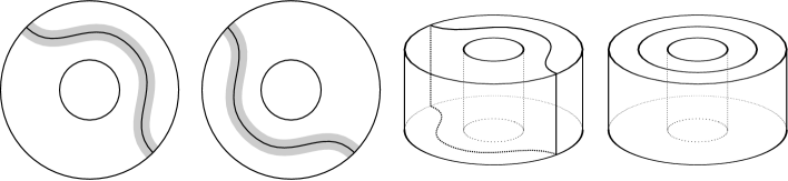
Figure 22. A partial open book for a standard neighborhood of an overtwisted disk. The shaded regions represent $P$ and $h(P)$. The two rightmost diagrams show the curves $\gamma$ and $\alpha^{\prime}$ in $\partial H(S)$, drawn as $(c\times\{1\})\cup(\partial c\times[-1,1])\cup(h(c)\times\{-1\})$ and $\alpha\times\{1\}$ in $S\times[-1,1]$.

∎

Remark 4.20.

With a bit of work, one should similarly be able to use Corollary 4.18 to prove that if $(M,\Gamma,\xi)$ has positive Giroux torsion, then $\psi(M,\Gamma,\xi)=0$ in analogy with [13].

Remark 4.21.

In [18], Honda, Kazez, and Matić define a map similar to $\Phi_{\xi,H}$ which depends only on $\xi$. We expect that our map $\Phi_{\xi,H}$ is likewise independent of $H$, as in Conjecture 1.7.

5. The bypass exact triangle

In this section, we work over the Novikov field $\mathcal{R}/2\mathcal{R}:=\mathcal{R}\otimes_{\mathbb{Z}}\mathbb{Z}/2\mathbb{Z}$ in order to use the surgery exact triangle in monopole Floer homology (see Remark 2.19). The results of the previous sections, including the construction and invariance of $\psi(M,\Gamma,\xi)$ and the definition of the contact handle attachment maps, hold over $\mathcal{R}/2\mathcal{R}$ without modification.

Suppose $(M,\Gamma)$ is a sutured manifold and $\alpha\subset\partial M$ is an arc which intersects $\Gamma$ in three points, including both endpoints of $\alpha$. A bypass move along $\alpha$ replaces $\Gamma$ with a new set of sutures $\Gamma^{\prime}$ which differ from $\Gamma$ in a neighborhood of $\alpha$, as shown in Figure 23.

2pt $\alpha$ at 22 28

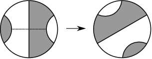
Figure 23. A bypass move along the arc $\alpha$.

If $\Gamma$ is the dividing set of a contact structure $\xi$ on $M$, then a bypass move is achieved by attaching an actual bypass along $\alpha$, as defined by Honda in [17]. In [39], Özbağcı observed that attaching a bypass along $\alpha$ is equivalent to first attaching a contact $1$-handle along disks in $\partial M$ centered at the endpoints of $\alpha$ and then attaching a contact $2$-handle along the union $\beta$ of $\alpha$ with an arc on the boundary of this $1$-handle, as shown in Figure 24. There is a canonical isotopy class of diffeomorphisms between the resulting manifold and $M$ which restrict to the identity outside a neighborhood of these handles. A bypass move along $\alpha$ thus gives rise to a morphism

$$\mathscr{H}_{\alpha}:\textbf{{\text@underline{SHM}}}(-M,-\Gamma)\to\textbf{{\text@underline{SHM}}}(-M,-\Gamma^{\prime})$$

which is the composition of the corresponding contact $1$- and $2$-handle maps with the map induced by this isotopy class of diffeomorphisms. Corollary 4.14 implies the following.

2pt $\alpha$ at 51 57 $\beta$ at 242 39

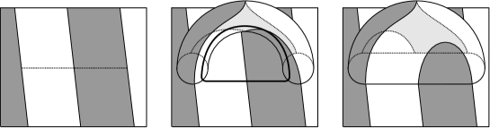
Figure 24. Performing a bypass move by attaching a contact $1$-handle at the endpoints of $\alpha$ and a contact $2$-handle along $\beta$.

Proposition 5.1.

Suppose $(M,\Gamma^{\prime},\xi^{\prime})$ is obtained from $(M,\Gamma,\xi)$ by attaching a bypass along $\alpha$ and pulling back the resulting contact structure to $M$ by the canonical isotopy class of diffeomorphisms. Then the induced map $\mathscr{H}_{\alpha}$ sends $\psi(M,\Gamma,\xi)$ to $\psi(M,\Gamma^{\prime},\xi^{\prime})$.

Figure 25 shows a sequence of bypass moves, performed in some fixed neighborhood in $\partial M$, resulting in a 3-periodic sequence of sutures on $M$. Such a sequence of bypass moves is what Honda calls a bypass triangle. Work-in-progress of Honda shows that a bypass triangle gives rise to a bypass exact triangle in sutured (Heegaard) Floer homology. The main result of this section is the analogous result in the monopole Floer setting, per the theorem below.

2pt $\alpha_{1}$ at 24 118 $\alpha_{2}$ at 148 117 $\alpha_{3}$ at 96 38 $\Gamma_{1}$ at -3 145 $\Gamma_{2}$ at 173 144 $\Gamma_{3}$ at 85 -8

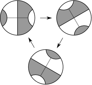
Figure 25. The bypass triangle. Each picture shows the attaching arc used to achieve the next set of sutures in the triangle.

Theorem 5.2.

Suppose $\Gamma_{1},\Gamma_{2},\Gamma_{3}\subset\partial M$ is the 3-periodic sequence of sutures resulting from successive bypass moves along arcs $\alpha_{1},\alpha_{2},\alpha_{3}$ as in Figure 25. Then the maps $\mathscr{H}_{\alpha_{1}},\mathscr{H}_{\alpha_{2}},\mathscr{H}_{\alpha_{3}}$ fit into an exact triangle

Proof.

We will prove Theorem 5.2 by realizing the bypass exact triangle as the usual surgery exact triangle in monopole Floer homology.

Note that by enlarging our local picture slightly, we can think of the arcs $\alpha_{1},\alpha_{2},\alpha_{3}$ as being arranged as in Figure 26 with respect to $\Gamma_{1}$. We may therefore view

$$(M,\Gamma_{2})\,\,\,{\rm and}\,\,\,(M,\Gamma_{3})\,\,\,{\rm and}\,\,\,(M,\Gamma_{1})$$

as being obtained from $(M,\Gamma_{1})$ by attaching bypasses along the arcs

$$\alpha_{1}\,\,\,{\rm and}\,\,\,\alpha_{1},\alpha_{2}\,\,\,{\rm and}\,\,\,\alpha_{1},\alpha_{2},\alpha_{3},$$

respectively. As described above, attaching a bypass along $\alpha_{i}$ amounts to attaching a contact $1$-handle $H_{i}$ along disks centered at the endpoints of $\alpha_{i}$ and then attaching a contact $2$-handle along a curve $\beta_{i}$ which extends $\alpha_{i}$ over the handle. Let $(Z_{1},\gamma_{1})$ be the sutured manifold obtained by attaching all three $H_{1},H_{2},H_{3}$ to $(M,\Gamma_{1})$, as in Figure 27. We will view $\beta_{1},\beta_{2},\beta_{3}$ as curves in $\partial Z_{1}$, as shown in the figure. For $i=1,2,3$, let $(Z_{i+1},\gamma_{i+1})$ be the result of attaching a contact $2$-handle to $(Z_{i},\gamma_{i})$ along $\beta_{i}$. We thus have the following canonical (up to isotopy) identifications:

$$(Z_{1},\gamma_{1}) \cong(M,\Gamma_{1})\cup H_{1}\cup H_{2}\cup H_{3}$$

$$(Z_{2},\gamma_{2}) \cong(M,\Gamma_{2})\cup H_{2}\cup H_{3}$$

$$(Z_{3},\gamma_{3}) \cong(M,\Gamma_{3})\cup H_{3}$$

$$(Z_{4},\gamma_{4}) \cong(M,\Gamma_{1}).$$

2pt $\alpha_{1}$ at 17 35 $\alpha_{2}$ at 32 51 $\alpha_{3}$ at 48 67

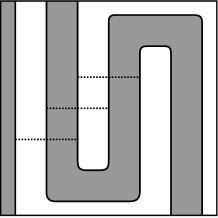
Figure 26. Another view of the arcs of attachment for the bypasses in the triangle. The suture drawn here is $\Gamma_{1}$.

2pt $\beta_{1}$ at 416 63 $\beta_{2}$ at 461 165 $\beta_{3}$ at 507 265 $a$ [B] at 974 95 $b$ [B] at 915 97

Figure 27. A view of $(Z_{1},\gamma_{1})$, obtained by attaching the contact 1-handles $H_{1},H_{2},H_{3}$ to $(M,\Gamma_{1}).$ Middle, the attaching curves $\beta_{1},\beta_{2},\beta_{3}$ for the contact $2$-handles. Right, the curves $a$ and $b$.

Recall that contact $1$-handle attachment has little effect on the level of closures. Specifically, if $\mathscr{D}=(Y,R,r,m,\eta)$ is a marked closure of sutured manifold after the $1$-handle attachment, then there is a marked closure of the sutured manifold before the $1$-handle attachment of the form $\mathscr{D}^{\prime}=(Y,R,r,m^{\prime},\eta)$. The corresponding $1$-handle attachment morphism is induced by the identity map from $\underline{SHM}(-\mathscr{D}^{\prime})$ to $\underline{SHM}(-\mathscr{D})$. We thus have canonical isomorphisms

$$\textbf{{\text@underline{SHM}}}(-Z_{i},-\gamma_{i})\cong\textbf{{\text@underline{SHM}}}(-M,-\Gamma_{i}),$$

for $i=1,2,3,4$, where the subscript of $\Gamma_{i}$ is taken mod $3$. In particular, $\textbf{{\text@underline{SHM}}}(-Z_{4},-\gamma_{4})$ is canonically identified with $\textbf{{\text@underline{SHM}}}(-Z_{1},-\gamma_{1})$. Therefore, to prove Theorem 5.2, it suffices to prove that there is an exact triangle

where $\mathscr{H}_{\beta_{i}}$ is the morphism associated to contact $2$-handle attachment along $\beta_{i}$.

Recall that on the level of closures, contact $2$-handle attachment corresponds to surgery. Specifically, if $\mathscr{D}_{i}=(Y_{i},R,r_{i},m_{i},\eta)$ is a marked closure of $(Z_{i},\gamma_{i})$, then there is a marked closure of $(Z_{i+1},\gamma_{i+1})$ of the form $\mathscr{D}_{i+1}=(Y_{i+1},R,r_{i+1},m_{i+1},\eta)$, where $Y_{i+1}$ is the result of $0$-surgery on $m_{i}(\beta_{i}^{\prime})$ with respect to the $(\partial Z_{i})$-framing, where $\beta_{i}^{\prime}$ is a pushoff of $\beta_{i}$ into the interior of $Z_{i}$. The morphism $\mathscr{H}_{\beta_{i}}$ is induced by the $2$-handle cobordism map

$$F_{i}:=\widecheck{\mathit{HM}}_{\bullet}({-}W_{i}|{-}R;\Gamma_{-\nu}):\underline{SHM}(-\mathscr{D}_{i})\to\underline{SHM}(-\mathscr{D}_{i+1})$$

corresponding to this surgery. So, to prove the exact triangle above, and, therefore, Theorem 5.2, it suffices to find a closure $\mathscr{D}_{1}$ of $(Z_{1},\gamma_{1})$ such that the surgeries relating the $-Y_{i}$ are exactly those that one encounters in the usual surgery exact triangle in monopole Floer homology. More precisely, it suffices to arrange that:

• $F_{1}$ is the map associated to $0$-surgery on some $K\subset-Y_{1}$,

• $F_{2}$ is the map associated to $(-1)$-surgery on a meridian $\mu_{1}\subset-Y_{2}$ of $K$,

• $F_{3}$ is the map associated to $(-1)$-surgery on a meridian $\mu_{2}\subset-Y_{3}$ of $\mu_{1}$.

Let $\mathscr{D}=(Y,R,r,m,\eta)$ be a marked closure of $(Z_{1},\gamma_{1})$. Let $a$ and $b$ be embedded curves in the positive and negative regions of $\partial Z_{1}$ as shown in Figure 27. Since neither curve intersects $\gamma_{1}$, we can assume that $a$ and $b$ are contained in $r(R\times\{-1\})$ and $r(R\times\{+1\})$, respectively. Let $Y_{1}$ be the manifold obtained from $Y$ by performing $(+1)$-surgeries on pushoffs $a^{\prime}$ and $b^{\prime}$ of $a$ and $b$ into the interior of $r(R\times[-1,1])$, with respect to their $\partial Z_{1}$-framings. Then $\mathscr{D}_{1}=(Y_{1},R,r_{1},m_{1},\eta)$ is a marked closure of $(Z_{1},\gamma_{1})$, where $m_{1}$ is the embedding induced by $m$ and $r_{1}$ is the canonical (up to isotopy) embedding induced by $r$. For ease of notation, we will think of the $m_{i}$ as being inclusions, and simply write $x$ for $m_{i}(x)$ for points $x\in Z_{i}$. In particular, $W_{i}$ is the 2-handle cobordism corresponding to $0$-surgery on $\beta_{i}^{\prime}\subset Y_{i}$.

2pt $\beta_{2}^{\prime\prime}$ at 457 515 $\beta_{3}^{\prime\prime}$ at 517 230

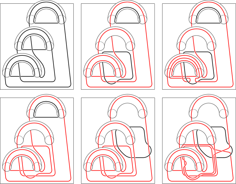
Figure 28. Top-left, the curves $\beta_{1}^{\prime},\beta_{2}^{\prime},\beta_{3}^{\prime},a^{\prime},b^{\prime}$ in a neighborhood of $\partial Z_{1}\subset Y$. Red indicates curves that have been surgered along. Top-middle, sliding $\beta^{\prime}_{2}\subset Y_{2}$ over $b^{\prime}$ to produce $\beta_{2}^{\prime\prime}$. Top-right, showing that $\beta_{2}^{\prime\prime}$ bounds a meridional disk of $\beta_{1}^{\prime}$ disjoint from the other surgery curves. Bottom-left, $\beta_{3}^{\prime}\subset Y_{3}$. Bottom-middle, sliding $\beta^{\prime}_{3}$ over $a^{\prime}$ and $\beta_{1}^{\prime}$ to produce $\beta_{3}^{\prime\prime}$. Bottom-right, showing that $\beta_{3}^{\prime\prime}$ bounds a meridional disk of $\beta_{2}^{\prime\prime}$ disjoint from the other surgery curves.

Recall that $Y_{2}$ is the result of $0$-surgery on $\beta_{1}^{\prime}\subset Y_{1}$. Let $\beta_{2}^{\prime\prime}$ be the curve in $Y_{2}$ obtained by handlesliding $\beta_{2}^{\prime}$ across the surgered curve $b^{\prime}$, as shown in the top-middle of Figure 28. Note that the $0$-framing on $\beta_{2}^{\prime}$ corresponds to the $(+1)$-framing on $\beta_{2}^{\prime\prime}$ under this isotopy. We may therefore think of $Y_{3}$ as the result of $(+1)$-surgery on $\beta_{2}^{\prime\prime}$ and $W_{2}$ as the corresponding 2-handle cobordism. We claim that $\beta_{2}^{\prime\prime}$ is a meridian of the surgered curve $\beta_{1}^{\prime}$. This is apparent once we handleslide the surgered curve $b^{\prime}$ over the surgered curve $\beta_{1}^{\prime}$, as shown in the top-right of Figure 28.

Let $\beta_{3}^{\prime\prime}$ be the curve in $Y_{3}$ obtained by handlesliding $\beta_{3}^{\prime}$ over the surgered curve $a^{\prime}$ and then over the surgered curve $\beta_{1}^{\prime}$, as shown in the bottom-middle of Figure 28. The $0$-framing on $\beta_{3}^{\prime}$ corresponds to the $(+1)$-framing on $\beta_{3}^{\prime\prime}$ under this isotopy, so we may therefore think of $Y_{4}\cong Y_{1}$ as the result of $(+1)$-surgery on $\beta_{3}^{\prime\prime}$ and $W_{3}$ as the corresponding 2-handle cobordism. We claim that $\beta_{3}^{\prime\prime}$ is a meridian of the surgered curve $\beta_{2}^{\prime\prime}$. This is apparent once we handleslide the surgered curve $a^{\prime}$ over the surgered curve $\beta_{2}^{\prime\prime}$, as shown in the bottom-right of Figure 28, noting that we are free to isotop $\beta_{2}^{\prime\prime}$ through the 1-handle $H_{2}$. It follows from these considerations that the maps $F_{1},F_{2},F_{3}$ are of the form described above for $K=\beta_{1}^{\prime}$, $\mu_{1}=\beta_{2}^{\prime\prime}$, $\mu_{2}=\beta_{3}^{\prime\prime}$. This completes the proof of Theorem 5.2. ∎

References

- [1] John A. Baldwin and Steven Sivek. Instanton Floer homology and contact structures.
- [2] John A. Baldwin and Steven Sivek. Invariants of Legendrian and transverse knots in monopole knot homology.
- [3] John A. Baldwin and Steven Sivek. Naturality in sutured monopole and instanton homology. 2013, math.GT/1305.4156.
- [4] J. Bloom. The combinatorics of Morse theory with boundary. In Proceedings of the 14th Gökova Geometry-Topology Conference, pages 43–88, 2012.
- [5] V. Colin, K. Honda, and P. Ghiggini. The equivalence of Heegaard Floer homology and embedded contact homology III: from hat to plus. 2012, math.SG/1208.1526.
- [6] V. Colin, K. Honda, and P. Ghiggini. The equivalence of Heegaard Floer homology and embedded contact homology via open book decompositions I. 2012, math.SG/1208.1074.
- [7] V. Colin, K. Honda, and P. Ghiggini. The equivalence of Heegaard Floer homology and embedded contact homology via open book decompositions II. 2012, math.SG/1208.1077.
- [8] Vincent Colin, Paolo Ghiggini, Ko Honda, and Michael Hutchings. Sutures and contact homology I. Geom. Topol., 15(3):1749–1842, 2011.
- [9] Tolga Etgü and Burak Özbağcı. Partial open book decompositions and the contact class in sutured Floer homology. Turkish J. Math., 33(3):295–312, 2009.
- [10] Tolga Etgü and Burak Ozbagci. On the relative Giroux correspondence. In Low-dimensional and symplectic topology, volume 82 of Proc. Sympos. Pure Math., pages 65–78. Amer. Math. Soc., Providence, RI, 2011.
- [11] J.B. Etnyre, D.S. Vela-Vick, and R. Zarev. Bordered sutured Floer homology and invariants of Legendrian knots. In preparation.
- [12] Hansjörg Geiges. An introduction to contact topology, volume 109 of Cambridge Studies in Advanced Mathematics. Cambridge University Press, Cambridge, 2008.
- [13] P. Ghiggini, K. Honda, and J. Van Horn-Morris. The vanishing of the contact invariant in the presence of torsion. 2007, math.GT/0706.1602.
- [14] E. Giroux. Convexité en topologie de contact. Comment. Math. Helv., 66:637–677, 1991.
- [15] Emmanuel Giroux. Structures de contact en dimension trois et bifurcations des feuilletages de surfaces. Invent. Math., 141(3):615–689, 2000.
- [16] K. Honda. Contact structures, Heegaard Floer homology and triangulated categories. In preparation.
- [17] K. Honda. On the classification of tight contact structures, I. Geom. Topol., 4:309–368, 2000.
- [18] Ko Honda, William H. Kazez, and Gordana Matić. Contact structures, sutured Floer homology and TQFT. 2008, arXiv:0807.2431.
- [19] Ko Honda, William H. Kazez, and Gordana Matić. The contact invariant in sutured Floer homology. Invent. Math., 176(3):637–676, 2009.
- [20] Michael Hutchings and Clifford Henry Taubes. Proof of the Arnold chord conjecture in three dimensions, II. Geom. Topol., 17(5):2601–2688, 2013.
- [21] A. Juhász and D. P. Thurston. Naturality and mapping class groups in Heegaard Floer homology. 2012, math.GT/1210.4996.
- [22] András Juhász. Cobordisms of sutured manifolds. 2009, math.GT/0910.4382.
- [23] Yutaka Kanda. On the Thurston-Bennequin invariant of Legendrian knots and nonexactness of Bennequin’s inequality. Invent. Math., 133(2):227–242, 1998.
- [24] P. Kronheimer and T. Mrowka. Monopoles and contact structures. Inv. Math., 130:209–255, 1997.
- [25] P. Kronheimer, T. Mrowka, P. Ozsváth, and Z. Szabó. Monopoles and lens space surgeries. Ann. Math., 165(2):457–546, 2007.
- [26] Peter Kronheimer and Tomasz Mrowka. Monopoles and three-manifolds, volume 10 of New Mathematical Monographs. Cambridge University Press, Cambridge, 2007.
- [27] Peter Kronheimer and Tomasz Mrowka. Knots, sutures, and excision. J. Differential Geom., 84(2):301–364, 2010.
- [28] C. Kutluhan. Seiberg-Witten knot homology via holonomy filtration. preprint.
- [29] C. Kutluhan, Y.-J. Lee, and C. H. Taubes. HF = HM I: Heegaard Floer homology and Seiberg-Witten Floer homology. 2010, math.SG/1007.1979.
- [30] C. Kutluhan, Y.-J. Lee, and C. H. Taubes. HF = HM II: Reeb orbits and holomorphic curves for the ech/Heegaard-Floer correspondence. 2010, math.SG/1008.1595.
- [31] C. Kutluhan, Y.-J. Lee, and C. H. Taubes. HF = HM III: Holomorphic curves and the differential for the ech/Heegaard-Floer correspondence. 2010, math.SG/1010.3456.
- [32] C. Kutluhan, Y.-J. Lee, and C. H. Taubes. HF = HM IV: The Seiberg-Witten Floer homology and ech correspondence. 2011, math.GT/1107.2297.
- [33] C. Kutluhan, Y.-J. Lee, and C. H. Taubes. HF = HM V: Seiberg-Witten Floer homology and handle additions. 2012, math.GT/1204.0115.
- [34] Yankı Lekili. Heegaard-Floer homology of broken fibrations over the circle. Adv. Math., 244:268–302, 2013.
- [35] Robert Lipshitz, Peter Ozsváth, and Dylan Thurston. Bordered Heegaard Floer homology: Invariance and pairing. 2008, math.GT/0810.0687.
- [36] Paolo Lisca, Peter Ozsváth, András I. Stipsicz, and Zoltán Szabó. Heegaard Floer invariants of Legendrian knots in contact three-manifolds. J. Eur. Math. Soc. (JEMS), 11(6):1307–1363, 2009.
- [37] P. Massot. Topological methods in 3-dimensional contact geometry. 2013, math.GT/1303.1063.
- [38] K. Niederkrüger and C. Wendl. Weak symplectic fillings and holomorphic curves. Ann. Sci. École Norm. Sup. (4), 44(5):801–853, 2011.
- [39] B. Ozbagci. Contact handle decompositions. Topology Appl., 158(5):718–727, 2011.
- [40] P. Ozsváth and Z. Szabó. Heegaard Floer homologies and contact structures. Duke Math. J., 129(1):39–61, 2005.
- [41] Steven Sivek. Monopole Floer homology and Legendrian knots. Geom. Topol., 16:751–779, 2012.
- [42] András I. Stipsicz and Vera Vértesi. On invariants for Legendrian knots. Pacific J. Math., 239(1):157–177, 2009.
- [43] C. H. Taubes. Embedded contact homology and Seiberg-Witten Floer cohomology, I. Geom. Topol., 14:2497–2581, 2010.
- [44] C. H. Taubes. Embedded contact homology and Seiberg-Witten Floer cohomology, II. Geom. Topol., 14:2583–2720, 2010.
- [45] C. H. Taubes. Embedded contact homology and Seiberg-Witten Floer cohomology, III. Geom. Topol., 14:2721–2817, 2010.
- [46] C. H. Taubes. Embedded contact homology and Seiberg-Witten Floer cohomology, IV. Geom. Topol., 14:2819–2960, 2010.
- [47] C. H. Taubes. Embedded contact homology and Seiberg-Witten Floer cohomology, V. Geom. Topol., 14:2961–3000, 2010.
- [48] Y. Tian. A categorification of as an algebra. 2012, math.QA/1210.5680.
- [49] Y. Tian. A categorification of and its tensor product representations. 2013, math.QA/1301.3986.
- [50] Y. Tian. A diagrammatic categorification of a Clifford algebra. 2013, math.QA/1309.6049.
- [51] Chris Wendl. A hierarchy of local symplectic filling obstructions for contact 3-manifolds. Duke Math. J., 162(12):2197–2283, 2013.
- [52] Rumen Zarev. Joining and gluing sutured Floer homology. 2010, arXiv:1010.3496.